Markov chain Monte Carlo (MCMC) methods
23
Markov chain Monte Carlo (MCMC) methods Gibbs Sampler I The Gibbs sampler is a conditional sampling technique in which the acceptance-rejection step is not needed. I The Markov transition rules of the algorithm are built upon conditional distributions derived from the target distribution. I Suppose that the random variable can be decomposed into n components, i.e. x =(x 1 x n ). In Gibbs sampler, one randomly or systematically chooses a coordinate x i and then substitutes it with x i drawn from π (x i | y x 1 x i -1 x i +1 x i +2 x n ) that is, the conditional posterior density of x i . I This conditional posterior usually is but does not have to be one-dimensional.
Transcript of Markov chain Monte Carlo (MCMC) methods

Markov chain Monte Carlo (MCMC) methodsGibbs SamplerI The Gibbs sampler is a conditional sampling techniquein which the acceptance-rejection step is not needed.I The Markov transition rules of the algorithm are builtupon conditional distributions derived from the targetdistribution.I Suppose that the random variable can be decomposedinto n components, i.e. x = (x1, . . . , xn). In Gibbs sampler,one randomly or systematically chooses a coordinate xiand then substitutes it with x ′i drawn from
π(xi | y , x1, . . . , xi−1, xi+1, xi+2, . . . , xn),that is, the conditional posterior density of xi .
I This conditional posterior usually is but does not have tobe one-dimensional.

Markov chain Monte Carlo (MCMC) methodsGibbs Sampler
Gibbs Sampler (Systematic Scan)1. Let k = 0 and x (0) = (x (0)
1 , x (0)2 , . . . , x (0)
n ).2. Draw x (k+1)i from the conditional density
π(xi | x (k+1)1 , . . . , x (k+1)
i−1 , x (k)i+1, . . . , x (k)
n ),for i = 1, . . . , n3. Set k = k + 1, and if k is less than total number ofiterations defined by the user, go back to the 2. step.

Markov chain Monte Carlo (MCMC) methodsGibbs SamplerGibbs Sampler (Random Scan)
1. Let t = 0 and x (0) = (x (0)1 , x (0)
2 , . . . , x (0)n ).2. Select a random uniformly distributed index i from theset {1, 2, . . . , n}.3. Draw x (k+1)
i from the conditional distributionπ(xi | x (k)
1 , . . . , x (k)i−1, x
(k)i+1, . . . , x (k)
n ).4. Set k = k + 1, and if k is less than total number ofiterations defined by the user, go back to the 2. step.

Markov chain Monte Carlo (MCMC) methodsGibbs Sampler
Metropolis-Hastings Gibbs samplerDifferences between the moves of Metropolis-Hastings(M-H) and Gibbs sampler (GS). In the images, the actualsamples have been visualized with red and the otherproposed (M-H) and conditional sampling (GS) points withblue.

Markov chain Monte Carlo (MCMC) methodsGibbs SamplerBalance Equation for Gibbs SamplerThe balance equation ∫ π(x)A(x , y ) dx = ∫ π(y )A(y , x) dx holdsfor Gibbs sampler, which can be shown as follows. Let usfor simplicity assume that the systematic scan Gibbs sampleris in question and each conditional density is aone-dimensional one. The transition function is given byA(x , y ) = n∏
i=1
π(yi | y1, . . . , yi−1, xi+1, . . . , xn).Integrating A(y , x) with respect to the last coordinate xn gives∫
RA(y , x)dxn = ∫
R
n∏i=1
π(xi | x1, . . . , xi−1, yi+1, . . . , yn)dxn

Markov chain Monte Carlo (MCMC) methodsGibbs SamplerBalance Equation for Gibbs Sampler continued= n−1∏
i=1
π(xi | x1, . . . , xi−1, yi+1, . . . , yn) ∫Rπ(xn | x1, . . . , xn−1)dxn
= n−1∏i=1
π(xi | x1, . . . , xi−1, yi+1, . . . , yn).The last equality follows from ∫
R π(xn | y1, . . . , yn−1)dxn = 1.Repeating this integration inductively with respect toxn−1, xn−2, . . . , x1, it follows that ∫Rn A(y , x)dx = 1. Thus, wehave ∫
Rnπ(y )A(y , x)dx = π(y )∫
RnA(y , x)dx = π(y ).

Markov chain Monte Carlo (MCMC) methodsGibbs SamplerBalance Equation for Gibbs Sampler continuedConsidering now the right-hand side of the balance equation,and observing that A(x , y ) is independent of x1, we have∫
Rnπ(x)A(x , y )dx1 = A(x , y ) ∫
Rnπ(x)dx1= A(x , y )π(x2, x3, . . . , xn),
and further ∫R π(x)A(x , y )dx1 =( n∏i=2
π(yi |y1, . . . , yi−1, xi+1, . . . , xn))π(y1 |x2, . . . , xn)π(x2, . . . , xn).

Markov chain Monte Carlo (MCMC) methodsGibbs SamplerBalance Equation for Gibbs Sampler continued= ( n∏
i=2
π(yi |y1, . . . , yi−1, xi+1, . . . , xn))π(y1, x2, x3, . . . , xn).Repeating this inductively for x2, x3, . . . , xn, and taking intoaccount that∫Riπ(y1, . . . , yi−1, xi , . . . , xn)π(yi | y1, . . . , yi−1, xi+1, . . . , xn)dxi= π(y1, . . . , yi−1, xi+1, . . . , xn)π(yi | y1, . . . , yi−1, xi+1, . . . , xn)= π(y1, . . . , yi−1, yi , xi+1, . . . , xn),
it follows that ∫Rn π(x)A(x , y )dx = π(y ), showing that thebalance equation holds.

Markov chain Monte Carlo (MCMC) methodsGibbs SamplerI In general, one step of Gibbs sampler (GS) requiresmore work than that of the Metropolis-Hastings (M-H)algorithm, since the former is likely to require morepoint evaluations of the posterior density.I However, subsequent points produced by GS are usuallyless mutually correlated than those produced by M-H,i.e. the sample ensemble of a given size is typicallybetter distributed according to the posterior in the caseof GS than that of M-H.I Sampling from a conditional density in Gibbs Samplertypically requires findind the essential part of the densitydue to which implementation can be difficult.

Markov chain Monte Carlo (MCMC) methodsGibbs SamplerSampling from one-dimensional densityOne can draw x distributed according to the probabilitydistribution Φ : R→ [0, 1], Φ(t) = ∫ t
−∞ π(τ) dτ , through thefollowing steps:1. Draw u from Uniform([0, 1]).2. Set x = Φ−1(u).I If the integral Φ(t) = ∫ t
−∞ π(τ) dτ is computed for a setof points t1, t2, . . . , tm covering the essential part of thesupport of π , the above algorithm can be used tonumerical sampling.

Markov chain Monte Carlo (MCMC) methodsGibbs SamplerNumerical sampling from one-dimensional densityOne can draw x distributed according to the probabilitydistribution Φ : R→ [0, 1], Φ(t) = ∫ t
−∞ π(τ) dτ , through thefollowing steps1. Find a set of points t1, t2, . . . , tm covering the essentialpart of the support of π.2. Compute the integral Φ(t) = ∫ t−∞ π(τ) dτ for each point
t1, t2, . . . , tm.3. Draw u from Uniform([0, 1]).4. Find the smallest index i for which Φ(ti ) > u and setx = ti .
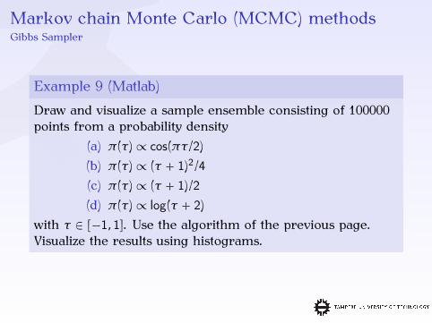
Markov chain Monte Carlo (MCMC) methodsGibbs SamplerExample 9 (Matlab)Draw and visualize a sample ensemble consisting of 100000points from a probability density(a) π(τ) ∝ cos(πτ/2)(b) π(τ) ∝ (τ + 1)2/4(c) π(τ) ∝ (τ + 1)/2(d) π(τ) ∝ log(τ + 2)with τ ∈ [−1, 1]. Use the algorithm of the previous page.Visualize the results using histograms.

Markov chain Monte Carlo (MCMC) methodsGibbs SamplerExample 9 (Matlab) continued
(a) (b)
(c) (d)Blue = Histogram, Red = Exact.

Markov chain Monte Carlo (MCMC) methodsGibbs SamplerExample 10 (Matlab)Repeat the sampling procedures of Example 9 using GibbsSampler. Compare the results to the ones obtained with therandom walk Metropolis with Gaussian proposals. Observethat the Gibbs sampler produces faster moving Markovchain than Metropolis-Hastings.SolutionSamples from each one-dimensional conditional densitywere produced numerically by dividing intersection of theunit disk and the line corresponding to conditional densityinto a 200 equally spaced points, and then the previouslygiven one-dimensional sampling algorithm was used.

Markov chain Monte Carlo (MCMC) methodsGibbs SamplerExample 10 (Matlab) continuedCase I: Three sensors, σ = 0.1
Posterior density Sample ensemble
horizontal component vertical componentpurple = exact, green = conditional mean, black = 95 % credibility

Markov chain Monte Carlo (MCMC) methodsGibbs SamplerExample 10 (Matlab) continuedCase I: Three sensors, σ = 0.1
Marginal density (horiz.) Marginal density (vertical)blue = sample based, red = exact
Burn in sequence (horiz.) Burn in sequence (vertical)purple = exact, green = conditional mean, black = 95 % credibility

Markov chain Monte Carlo (MCMC) methodsGibbs SamplerExample 10 (Matlab) continuedCase II: Three sensors, σ = 0.2
Posterior density Sample ensemble
horizontal component vertical componentpurple = exact, green = conditional mean, black = 95 % credibility

Markov chain Monte Carlo (MCMC) methodsGibbs SamplerExample 10 (Matlab) continuedCase II: Three sensors, σ = 0.2
Marginal density (horiz.) Marginal density (vertical)blue = sample based, red = exact
Burn in sequence (horiz.) Burn in sequence (vertical)purple = exact, green = conditional mean, black = 95 % credibility

Markov chain Monte Carlo (MCMC) methodsGibbs SamplerExample 10 (Matlab) continuedCase III: Five sensors, σ = 0.1
Posterior density Sample ensemble
horizontal component vertical componentpurple = exact, green = conditional mean, black = 95 % credibility

Markov chain Monte Carlo (MCMC) methodsGibbs SamplerExample 10 (Matlab) continuedCase III: Five sensors, σ = 0.1
Marginal density (horiz.) Marginal density (vertical)blue = sample based, red = exact
Burn in sequence (horiz.) Burn in sequence (vertical)purple = exact, green = conditional mean, black = 95 % credibility

Markov chain Monte Carlo (MCMC) methodsGibbs SamplerExample 10 (Matlab) continuedCase IV: Five sensors, σ = 0.2
Posterior density Sample ensemble
horizontal component vertical componentpurple = exact, green = conditional mean, black = 95 % credibility

Markov chain Monte Carlo (MCMC) methodsGibbs SamplerExample 10 (Matlab) continuedCase IV: Five sensors, σ = 0.2
Marginal density (horiz.) Marginal density (vertical)blue = sample based, red = exact
Burn in sequence (horiz.) Burn in sequence (vertical)purple = exact, green = conditional mean, black = 95 % credibility

Markov chain Monte Carlo (MCMC) methodsGibbs SamplerExample 10 (Matlab) continued
I Based on the burn in sequence, it is clear that the Gibbssampler produces a faster moving Markov chain thanthe Metropolis-Hastings, i.e. the sample points are lessmutually correlated in the case of Gibbs sampler.I A rule of thumb is that the more the sampling historyfor a single coordinate looks like a "fuzzy worm" themore independent are the sampling points and thebetter is the Markov chain in general with regard toconvergence of the estimates.