Bootstrap confidence intervals: when, which, what? …saharon/Boot/10.1.1.133.8405.pdfSTATISTICS IN...

STATISTICS IN MEDICINEStatist. Med. 2000; 19:1141}1164

Bootstrap con"dence intervals: when, which, what?A practical guide for medical statisticians

James Carpenter1,* and John Bithell2

1 Medical Statistics Unit, London School of Hygiene and Tropical Medicine, Keppel Street, London WC1E 7HT, U.K.2 Department of Statistics, 1 South Parks Road, Oxford, OX1 3TG, U.K.

SUMMARY

Since the early 1980s, a bewildering array of methods for constructing bootstrap con"dence intervals havebeen proposed. In this article, we address the following questions. First, when should bootstrap con"denceintervals be used. Secondly, which method should be chosen, and thirdly, how should it be implemented. Inorder to do this, we review the common algorithms for resampling and methods for constructing bootstrapcon"dence intervals, together with some less well known ones, highlighting their strengths and weaknesses.We then present a simulation study, a #ow chart for choosing an appropriate method and a survival analysisexample. Copyright ( 2000 John Wiley & Sons, Ltd.

1. INTRODUCTION: CONFIDENCE INTERVALS AND COVERAGE ERROR

An accurate estimate of the uncertainty associated with parameter estimates is important to avoidmisleading inference. This uncertainty is usually summarized by a con"dence interval or region,which is claimed to include the true parameter value with a speci"ed probability. In this paper weshall restrict ourselves to con"dence intervals. We begin with an example which illustrates whywe might want bootstrap con"dence intervals.

1.1. Example: Remission from acute myelogenous leukaemia

Embury et al. [1] conducted a clinical trial to evaluate the e$cacy of maintenance chemotherapyfor acute myelogenous leukaemia. Twenty-three patients who were in remission after treatmentwith chemotherapy were randomized into two groups. The "rst group continued to receivemaintenance chemotherapy, while the second did not. The objective of the trial was to examinewhether maintenance chemotherapy prolonged the time until relapse. The preliminary results ofthe study are shown in Table I. We wish to test the hypothesis that maintenance chemotheraphydoes not delay relapse by constructing a con"dence interval for the treatment e!ect.

*Correspondence to: James Carpenter, Medical Statistics Unit, London School of Hygiene and Tropical Medicine,Keppel Street, London WC1E 7HT, U.K.

Received January 1998Copyright ( 2000 John Wiley & Sons, Ltd. Accepted August 1999

Table I. Remission times (weeks) forpatients with acute myelogenous leukae-mia; group 1 with maintenance chemo-therapy; group 2 none. An entry suchas'13 means that the only informationavailable is that at 13 weeks the patient

was still in remission.

Treat 1 Treat 2

9 513 5

'13 818 812 1223 '1631 2334 27

'45 3048 33

'161 4345

Figure 1. Plot of non-parametric estimate of cumulative hazard function for the data in Table I, on a log-logscale. The upper line corresponds to treatment group 2.

Figure 1 shows a log-log plot of the cumulative hazard function, and suggests that a propor-tional hazards model

h(t)"h0(t) exp(bx)

1142 J. CARPENTER AND J. BITHELL

Copyright ( 2000 John Wiley & Sons, Ltd. Statist. Med. 2000; 19:1141}1164

will be adequate, where h (t) is the hazard at time t, h0( ) ) is the baseline hazard and x is an

indicator covariate for treatment 2. Fitting this model gives bK "0.924 with standard errorp("0.512. A standard 95 per cent normal approximation con"dence interval for b is thereforebK $1.96]0.512, that is, (!0.080, 1.928).

However, the accuracy of this interval depends on the asymptotic normality of bK and thisassumption is questionable with so few observations. Accordingly, we may want to constructa con"dence interval that does not depend on this assumption. Bootstrapping provides a ready,reliable way to do this. The principal questions are which bootstrap con"dence interval methodshould be chosen and what should be done to implement it. These are the questions this articleseeks to answer in a practical context, by reviewing the methods available, highlighting theirmotivation, strengths and weaknesses. After doing this, we return to this example in Section 7.

We begin by de"ning coverage error, which is a key concept in comparing bootstrap con"denceinterval methods. Suppose (!R, h

U) is, for example, a normal approximation con"dence inter-

val, with nominal coverage 100(1!a) per cent (a typically 0.05). Then it will often have a coverageerror so that

P (h(hU)"(1!a)#C

for some unknown constant C, where typically CP0 as n, the sample size, PR.Bootstrap con"dence intervals aim to reduce this coverage error by using simulation to avoid

the assumptions inherent in classical procedures. While they are often calculated for small datasets (for example, to check on the assumption of asymptotic normality), they are equallyapplicable to large data sets and complex models; see for example Carpenter [2] and LePage andBillard [3].

Thus, bootstrap con"dence intervals will at the least validate the assumptions necessary toconstruct classical intervals, while they may further avoid misleading inferences being drawn. Theway they go about this, and the extent on which they succeed, are described in Sections 2 and3 and illustrated in Sections 5 and 7. First, however, we describe the bootstrap principle and theterms non-parametric and parametric simulation.

In many statistical problems we seek information about the value of a population parameterh by drawing a random sample Y from that population and constructing an estimate hK (Y) of thevalue of h from that sample. The bootstrap principle is to obtain information about therelationship between h and the random variable hK (Y) by looking at the relationship betweenhK (y

0"4) and hK (Y*), where Y* is a resample characterized by the sample y

0"4. Y* can either be

constructed by sampling with replacement from the data vector y0"4

, the so-called non-parametricbootstrap, or by sampling from the distribution function parameterized by hK (y

0"4), the so-called

parametric bootstrap.Before we discuss the various methods for bootstrap con"dence interval construction, we give

algorithms for non-parametric and parametric simulation, and illustrate these in a regressioncontext, where the bootstrap is frequently applied.

2. RESAMPLING PLANS

Here we give algorithms for non-parametric and semi-parametric resampling plans, and illustratethem with a linear model example. We "rst describe this example.

BOOTSTRAP CONFIDENCE INTERVALS 1143


Table II. Weights of 14 babies at birth and 70}100 days. From Armitageand Berry (Reference [4], p. 148).

Case number Birthweight (oz) Weight at 70}100 days (oz)

1 72 1212 112 1833 111 1844 107 1845 119 1816 92 1617 126 2228 80 1749 81 178

10 84 18011 115 14812 118 16813 128 18914 128 192

Figure 2. Plot of data in Table II, with least squares regression line 70}100 day weight"a#b]birth-weight. Estimates (standard errors) are bK "0.68 (0.28), a("104.89 (29.65).

Table II gives the weight at birth and 70}100 days of 14 babies, from Armitage and Berry(Reference [4], p. 148). The data are plotted in Figure 2, together with the least squares regressionline. Parameter estimates are given in the caption. It appears that there is a borderline associationbetween birthweight and weight at 70}100 days. However, the data set is small, and we may wishto con"rm our conclusions by constructing a bootstrap con"dence interval for the slope. To dothis, we "rst need to construct bootstrap versions bK *, of b. We now outline how to do thisnon-parametrically and parametrically.



2.1. Non-parametric resampling

Non-parametric resampling makes no assumptions concerning the distribution of, or model for,the data. Our data is assumed to be a vector y

0"4of n independent observations, and we are

interested in a con"dence interval for hK (y0"4

). The general algorithm for a non-parametricbootstrap is as follows:

1. Sample n observations randomly with replacement from y0"4

to obtain a bootstrap data set,denoted Y*.

2. Calculate the bootstrap version of the statistic of interest, hK *"hK (Y*).3. Repeat steps 1 and 2 a large number of times, say B, to obtain an estimate of the bootstrap

distribution.

We discuss the value of B appropriate for con"dence intervals in Section 2.4.In the context of the birthweight data in Table II, each &observation' in the original data set

consists of a pair, or case, (x, y). For example, the "rst case is (72, 121). The algorithm thenproceeds as follows:

1. Sample n cases randomly with replacement to obtain a bootstrap data set. Thus, a typicalbootstrap data set might select the following cases:

4 5 2 4 9 10 3 3 6 2 1 6 9 8.

2. Fit the linear model to the bootstrap data and obtain the bootstrap slope, bK *. For thespeci"c bootstrap data set in step 1, bK *"0.67.

3. Repeat steps 1 and 2 a large number, say B, of times to obtain an estimate of the bootstrapdistribution.

The bootstrap slopes bK *1, 2 , bK *

B, can then be used to form a non-parametric bootstrap con"-

dence interval for b as described in Section 3.

2.2. Parametric resampling

In parametric resampling we assume that a parametric model for the data, FY(y ; . ), is known up

to the unknown parameter vector, h, so that bootstrap data are sampled from FY(y ; hK ), where hK is

typically the maximum likelihood estimate from the original data. More formally, the algorithmfor the parametric bootstrap is as follows:

1. Let hK be the estimate of h obtained from the data (for example, the maximum likelihoodestimate). Sample n observations, denoted Y* from the model F

Y( . ; hK ).

2. Calculate hK *"hK (Y*).3. Repeat 1 and 2 B times to obtain an estimate of the parametric bootstrap distribution.

In the linear model example, &assuming the model' means treating the assumptions of the linearmodel as true, that is, assuming that the x1s (the birthweights) are known without error and thatthe residuals are normally distributed with mean zero and variance given by the residual standarderror, which is p2"14.1. We then sample n"14 residuals and pass these back through the modelto obtain the bootstrap data. The algorithm is as follows:

1. Draw n observations, z1, 2 , z

14, from the N(0, p2) distribution.



2. Calculate bootstrap responses, y*i, as y*

i"a(#bK x

i#z

i, i31, 2 , 14. For example, if

z1"31.2

y*1"104.89#0.68]72#31.2"185.05.

The bootstrap data set then consists of the n"14 pairs (y*i, x

i).

3. Calculate the bootstrap slope, bK *, as the least squares regression slope for this bootstrapdata set.

4. Repeat 1}3 B times to obtain an estimate of the parametric bootstrap distribution.

As before, the resulting bootstrap sample, bK *1, 2 , bK *

B, can be used to construct a bootstrap

con"dence interval.

2.3. Semi-parametric resampling

This resampling plan is a variant of parametric resampling, appropriate for some forms ofregression. Since it involves non-parametric resampling of the residuals from the "tted parametricmodel, we term it semi-parametric resampling. As before, we begin with a general presentation.

Suppose we have responses y"(y1, 2 , y

n) with covariates x"(x

1, 2 , x

n), and we "t the

model

y"g (b, x)#r

obtaining estimates bK of the parameters b and a set of residuals ri, i3(1, 2 , n).

Without loss of generality, suppose we are interested in a con"dence interval for b1. The

algorithm for semi-parametric resampling is as follows:

1. Adjust the residuals r"(r1, 2 , r

n) so that they have approximately equal means and

variances. Denote this new set by (rJ1, 2 , rJ

n).

2. Sample with replacement from the set of adjusted residuals (rJ1, 2 , rJ

n) to obtain a set of

bootstrap errors, r*"(rJ *1, 2 , rJ *

n).

3. Then obtain bootstrap data y*"(y*1, 2 , y*

n) by setting

y*"g (bK , x)#r*.

4. Next "t the model,

Ey*"g (b, x)

to obtain the bootstrap estimate bK *.5. Repeat steps 1}4 above B times to obtain an estimate of the bootstrap distribution.

It is important to note that this resampling plan is only appropriate when it is reasonable toassume that the adjusted residuals, rJ

i, are independent and identically distributed (henceforth

i.i.d.). If this is reasonable, then this resampling plan is usually preferable to the straightparametric plan, as it does not force the residuals to conform to a known distribution.

However, if the rJi, are not i.i.d. so that, for example, the variance of y depends on its mean, then

this must be modelled, and the sampling algorithm revised. An algorithm for this situation isgiven by Davison and Hinkley (Reference [5], p. 271).



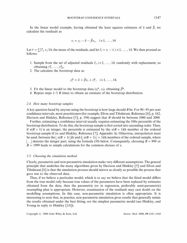
In the linear model example, having obtained the least squares estimates of a( and b) , wecalculate the residuals as

ri"y

i!aL !bK x

i, i31, 2 , 14

Let rN"+14i/1

ri/14, the mean of the residuals, and let rJ

i"r

i!rN , i31, 2 , 14. We then proceed as

follows:

1. Sample from the set of adjusted residuals rJi, i31, 2 , 14, randomly with replacement, so

obtaining r*1, 2 , r*

14.

2. The calculate the bootstrap data as

y*i"aL #bK x

i#r*

i, i31, 2 , 14.

3. Fit the linear model to the bootstrap data (y*i, x

i), obtaining bK *.

4. Repeat steps 1}3 B times to obtain an estimate of the bootstrap distribution.

2.4. How many bootstrap samples

A key question faced by anyone using the bootstrap is how large should B be. For 90}95 per centcon"dence intervals, most practitioners (for example, Efron and Tibshirani, Reference [6], p. 162,Davison and Hinkley, Reference [5], p. 194) suggest that B should be between 1000 and 2000.

Further, estimating a con"dence interval usually requires estimating the 100a percentile of thebootstrap distribution. To do this, the bootstrap sample is "rst sorted into ascending order. Then,if a (B#1) is an integer, the percentile is estimated by the a (B#1)th member of the orderedbootstrap sample (Cox and Hinkley, Reference [7], Appendix A). Otherwise, interpolation mustbe used, between the xa (B#1)yth and (xa (B#1)y#1)th members of the ordered sample, wherex.y denotes the integer part, using the formula (10) below. Consequently, choosing B"999 orB"1999 leads to simple calculations for the common choices of a.

2.5. Choosing the simulation method

Clearly, parametric and non-parametric simulation make very di!erent assumptions. The generalprinciple that underlies the many algorithms given by Davison and Hinkley [5] and Efron andTibshirani [6] is that the simulation process should mirror as closely as possible the process thatgave rise to the observed data.

Thus, if we believe a particular model, which is to say we believe that the "tted model di!ersfrom the true model only because true values of the parameters have been replaced by estimatesobtained from the data, then the parametric (or in regression, preferably semi-parametric)resampling plan is appropriate. However, examination of the residuals may cast doubt on themodelling assumptions. In this case, non-parametric simulation is often appropriate. It isinteresting to note that, in practice, non-parametric simulation gives results that generally mimicthe results obtained under the best "tting, not the simplest parametric model (see Hinkley, andYoung in reply to Hinkley [5,8]).



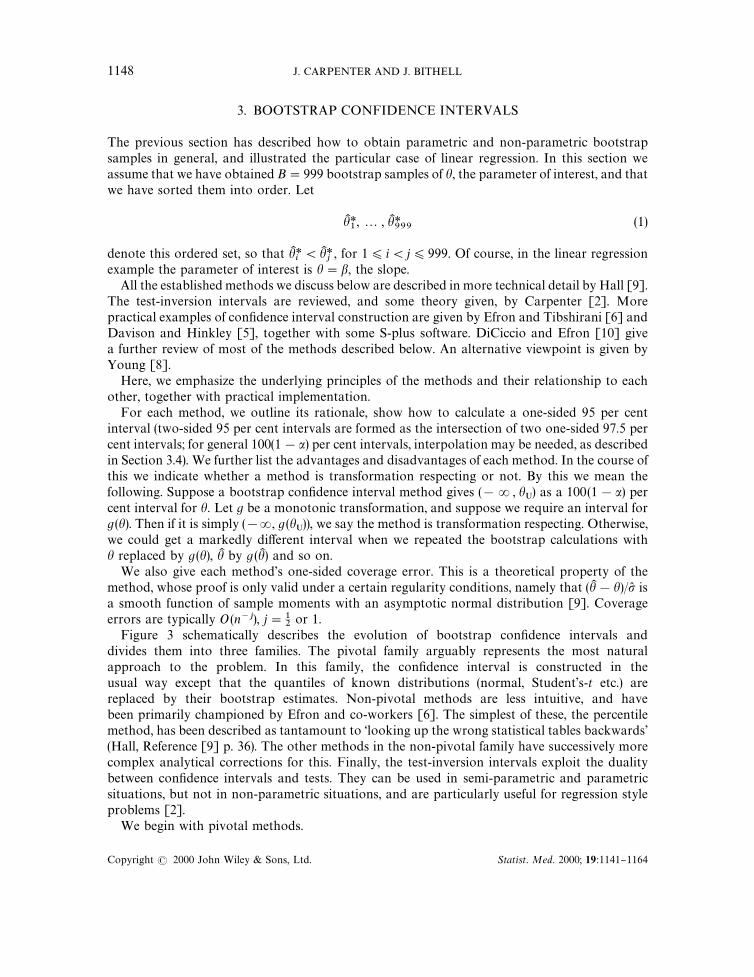
3. BOOTSTRAP CONFIDENCE INTERVALS

The previous section has described how to obtain parametric and non-parametric bootstrapsamples in general, and illustrated the particular case of linear regression. In this section weassume that we have obtained B"999 bootstrap samples of h, the parameter of interest, and thatwe have sorted them into order. Let

hK *1, 2 , hK *

999(1)

denote this ordered set, so that hK *i(hK *

j, for 1)i(j)999. Of course, in the linear regression

example the parameter of interest is h"b, the slope.All the established methods we discuss below are described in more technical detail by Hall [9].

The test-inversion intervals are reviewed, and some theory given, by Carpenter [2]. Morepractical examples of con"dence interval construction are given by Efron and Tibshirani [6] andDavison and Hinkley [5], together with some S-plus software. DiCiccio and Efron [10] givea further review of most of the methods described below. An alternative viewpoint is given byYoung [8].

Here, we emphasize the underlying principles of the methods and their relationship to eachother, together with practical implementation.

For each method, we outline its rationale, show how to calculate a one-sided 95 per centinterval (two-sided 95 per cent intervals are formed as the intersection of two one-sided 97.5 percent intervals; for general 100(1!a) per cent intervals, interpolation may be needed, as describedin Section 3.4). We further list the advantages and disadvantages of each method. In the course ofthis we indicate whether a method is transformation respecting or not. By this we mean thefollowing. Suppose a bootstrap con"dence interval method gives (!R, h

U) as a 100(1!a) per

cent interval for h. Let g be a monotonic transformation, and suppose we require an interval forg(h). Then if it is simply (!R, g (h

U)), we say the method is transformation respecting. Otherwise,

we could get a markedly di!erent interval when we repeated the bootstrap calculations withh replaced by g(h), hK by g (hK ) and so on.

We also give each method's one-sided coverage error. This is a theoretical property of themethod, whose proof is only valid under a certain regularity conditions, namely that (hK !h)/p( isa smooth function of sample moments with an asymptotic normal distribution [9]. Coverageerrors are typically O(n~j), j"1

2or 1.

Figure 3 schematically describes the evolution of bootstrap con"dence intervals anddivides them into three families. The pivotal family arguably represents the most naturalapproach to the problem. In this family, the con"dence interval is constructed in theusual way except that the quantiles of known distributions (normal, Student's-t etc.) arereplaced by their bootstrap estimates. Non-pivotal methods are less intuitive, and havebeen primarily championed by Efron and co-workers [6]. The simplest of these, the percentilemethod, has been described as tantamount to &looking up the wrong statistical tables backwards'(Hall, Reference [9] p. 36). The other methods in the non-pivotal family have successively morecomplex analytical corrections for this. Finally, the test-inversion intervals exploit the dualitybetween con"dence intervals and tests. They can be used in semi-parametric and parametricsituations, but not in non-parametric situations, and are particularly useful for regression styleproblems [2].

We begin with pivotal methods.



Figure 3. Schematic diagram describing relationship of bootstrap methods for constructing con"denceintervals, with early references. Consistent coverage means the coverage error is O(n~1@2); ,rst-order correct

coverage means the coverage error is O(n~1). See the introduction and Table III for more details.

3.1. Non-Studentized pivotal method (sometimes called *basic+)

3.1.1. Rationale. Arguably the most natural way of setting about constructing a con"denceinterval for h is to seek a function of the estimator and parameter whose distribution isknown, and then use the quantiles of this known distribution to construct a con"dence intervalfor the parameter. However, in the absence of detailed knowledge about the distribution F

Y( . ; h)

from which the observations are drawn, it is not clear which function of the parameter andestimator should be chosen. Indeed, the procedure outlined below could, in principle, be appliedto any statistic="g(#) ; h), provided g is continuous. However, in view of the fact that manyestimators are asymptotically normally distributed about their mean, it makes sense to use="#) !h.

Suppose that the distribution of = were known, so that we could "nd wa such thatP (=)wa )"a. Then a one-sided 100(1!a) per cent con"dence interval for h would be

(!R, hK !wa) (2)

The problem is that, in practice, the distribution of = is not known. However, the bootstrapprinciple implies that we can learn about the relationship between the true parameter value h andthe estimator hK by pretending that hK is the true parameter value and looking at the relationshipbetween hK and estimates of hK , denoted by hK *, which we construct from data simulated from themodel parameterized by hK .

In other words, the bootstrap procedure tells us to replace the quantile, wa , of= in (2) with theappropriate quantile, w*a , of=*"(#) *!hK ), calculated as described below. The non-Studentizedpivotal interval is thus

(!R, hK !w*a ) (3)



3.1.2. Calculation of 95 per cent interval. Recall we have already calculated and ordered ourbootstrap sample (1).

1. Set w*i"hK *

i!hK , for i31, 2 , 999.

2. The 0.05th quantile of =* is then estimated by w*j, where j"0.05](999#1)"50.

3. The one-sided 95 per cent con"dence interval is thus

(!R, hK !wL *50

)

Note that there are two distinct sources of error in this procedure. The "rst, termed bootstraperror, arises from appealing to the bootstrap principle to replace the quantile of= in (2) with thatof=*. The second, termed Monte Carlo error, arises because Monte Carlo simulation is used toestimate the 100ath percentile of=* (steps 1 and 2 above). Provided the number of simulations instep 2 is su$ciently large, (see Section 2.4), the Monte Carlo error is usually negligible comparedto the bootstrap error. The accuracy of the method therefore depends critically on the similarityof the distributions of = and =*. Unfortunately, these are generally not close (Davison andHinkley, Reference [5], p. 211).

3.1.3. Advantages. Often provides an accurate, simple to calculate, con"dence interval for thesample median (Davison and Hinkley, Reference [5], p. 42).

3.1.4. Disadvantages. Typically substantial coverage error because the distributions of = and=* di!er markedly. If there is a parameter constraint (such as h'0) then the interval oftenincludes invalid parameter values.

3.1.5. Coverage error [9].

P (hK !w*a'h)"1!a#O(n~1@2)

3.2. Bootstrap-t method (Studentized pivotal)

3.2.1. Rationale. As discussed above, the non-Studentized pivotal method is generally unreliablebecause the distributions of= and =* di!er markedly. If y

0"4were a sample from the normal

distribution, then the reason for this would be that the variance of=would not equal that of=*.Denote an estimate of the standard deviation of hK by p( . Then the obvious way around thisdi$culty would be to work with ¹"(hK !h)/p( instead of =. The bootstrap-t method is justa generalization of this principle. Thus the interval (3) becomes

(!R, hK !p( t*a ) (4)

where t*a is the 100ath percentile of ¹*"(hK *!hK )/pL *, the bootstrap version of ¹.

3.2.2. Calculation of 95 per cent interval. To use this method, an estimate of the standard error ofeach hK *

iin (1) has to be calculated, for every i. For instance, if hK (y)"+n

i/1yi/n, the sample mean,

then p( 2(hK )"+ni/1

(yi!hK (y))2/n(n!1). For more complicated statistics, estimating p can be

problematic, although a variety of approximations exist. A moderately technical review is givenby Davison and Hinkley Reference [5], Chapters 2 and 3. In regression problems, however, the



standard error of the parameters is readily available. In our simple linear regression example, it isgiven by

Residual standard error

+ni/1

(xi!xN )2

For the calculations below, we therefore assume that for each member of the bootstrap sample (1)we have calculated the corresponding standard error p( *

i, i31, 2 , B. We then proceed as follows:

1. Set t*i"(hK *

i!hK )/p( *

i, i31, 2 , 999"B. Order this set of t*

i's.

2. Denote by tK *50

the 50th largest t* (where 50"0.05](B#1)).3. The con"dence interval is then

(!R, hK !p( tK *50

).

As already discussed, this method clearly depends on being able to calculate p( . In many problems,for this method to be computationally feasible, an analytic form of p( must be known. However,for some statistics, even analytic approximations to p( may prove elusive. In this case, one option[5] is to carry out a computationally heavy, but routine, &second level bootstrap' to estimate p( * asfollows.

From y*i

obtain, using either parametric or non-parametric simulation, M y**'s and thecorresponding values of hK **"hK (y**). Then the variance of hK (y*

i) is estimated by

p( *2"1

M!1

M+j/1

(hK **j

!hK (y*i))2

This procedure must be repeated for each of the B hK *'s. Finally, the variance of hK (y0"4

) can beestimated by

p( 2"1

B!1

B+i/1

(hK *i!hK (y

0"4))2

Usually, M"25 is su$cient for each of these second level bootstraps. Clearly though, thisprocess is computationally heavy, as for every simulation required for the basic bootstrap-tmethod, a further M are now required, making MB altogether.

An additional problem with this method is that it will perform very poorly if p( is not (at leastapproximately) independent of hK . This assumption can easily be checked by plotting p( * againsthK *, as shown in Section 7. If it is violated, we construct the variance stabilized bootstrap-t interval,as follows:

1. Use either parametric or non-parametric simulation to obtain B pairs (hK *, p( *), together witha second set of B hK *'s.

2. Use a non-linear regression technique on the B pairs to estimate the function s such thatp( *"s(hK *). Having estimated s, use numerical integration to estimate f (x)":x 1/s (h) dh.A Taylor series expansion shows that f is the approximate variance stabilizing transforma-tion.

3. Transform the (hitherto unused) B hK *'s to the variance stabilized scale. Since the variance isnow assumed stable, we can construct a non-Studentized pivotal interval for f (h).

4. Finally, calculate an estimate of f~1 and back transform the interval obtained in step 3 tothe original scale.



In spite of all the numerical calculations, the variance stabilized bootstrap-t interval usuallyalleviates the problems of the bootstrap-t when the variance of hK * is not constant (Efron andTibshirani, Reference [6], p. 162 ! ; Carpenter [2]).

3.2.3. Advantages. Provided p( is easily available, the method performs reliably in many exam-ples, in both its standard and variance stabilized forms (see Davison and Hinkley, Reference [5],p. 231, for a simulation study and references to others).

3.2.4. Disadvantages. The method is computationally very intensive if p( * is calculated usinga double bootstrap. Intervals can include invalid parameter values and it is not transformationrespecting.


P (h!p( t*a'h)"1!a#O(n~1)

3.3. Percentile Method

We now move to the second arm of Figure 3. These methods are in some ways less intuitive thanthose described above, but have the advantage of not requiring p( .

3.3.1. Rationale. Consider a monotonically increasing function g ( . ), and write /"g(h), /K "g(hK )and /K *"g(hK *). Choose (if possible) g ( . ), such that

/K *!/K &/K !/&N(0, p2) (5)

Then, since /K !/&N(0, p2), the interval for h is

(!R, g~1(/K !pza)) (6)

where za is the 100a per cent point of the standard normal distribution. However, (5) implies that/K !pza"F~1

(K *(1!a). Further, since g is monotonically increasing, F~1

(K *(1!a)"g (F~1hK * (1!a)).

Substituting in (6) gives the percentile interval

(!R, F~1hK * (1!a)) (7)

3.3.2. Calculation of 95 per cent interval. Recall the set of B"999 bootstrap samples (1). Theupper end point of the one-sided 95 per cent percentile interval is F~1hK * (0.95), which is estimated bythe 950th member of (1), since 950"0.95](B#1). The percentile interval is then

(!R, hK *950

)

3.3.3. Advantages. Simplicity is the attraction of this method, and explains its continued popula-rity. Unlike the bootstrap-t, no estimates of the p are required. Further, no invalid parametervalues can be included in the interval.

Another advantage of this group of methods over the pivotal methods is that they aretransformation respecting.

3.3.4. Disadvantages. The coverage error is often substantial if the distribution of hK is not nearlysymmetric (Efron and Tibshirani, Reference [6], p. 178 ! ). The reason is that the justi"cation of



the method rests on the existence of a g ( . ) such that (5) holds, and for many problems sucha g does not exist.


P(hK *1~a'h)"1!a#O(n~1@2)

3.4. Bias corrected method

The quickly recognized shortcomings of the percentile method [11] led to the development of thebias corrected or BC method.

3.4.1. Rationale. Again, consider a monotonically increasing function g ( . ), and write /"g (h),/K "g(hK ) and /K *"g(hK *). However, now (if possible) choose g ( . ), such that

/K *!/K &/K !/&N(!bp, p2) (8)

for some constant b. An analogous (but slightly more complex) argument than that used in thecase of the percentile interval then yields the BC interval

(!R, F~1h) * ('(2b!za))) (9)

where b is estimated by '~1 (P (hK *)hK )) and '~1 is the inverse cumulative distribution functionof the normal distribution.

3.4.2. Calculation of 95 per cent interval.

1. Count the number of members of (1) that are less than hK (calclated from the original data).Call this number p and set b"'~1(p/B).

2. Calculate Q"(B#1)'(2b!z0.05

), where z0.05

"!1.64. Q is the percentile of the boot-strap distribution required for the upper endpoint of the bias corrected con"dence interval.

3. Estimate the endpoint of the interval by h) *xQy , where x.y means &take the integer part'. Ifa more accurate estimate is required, interpolation can be used between the members of (1),as follows. Let the nearest integers to Q be a, b, so that a(Q(b and b"a#1. Then theQth percentile is estimated by

hK *Q+hK *

a#

'~1 ( QB`1

)!'~1 ( aB`1

)

'~1 ( bB`1

)!'~1 ( aB`1

)(hK *

b!hK *

a) (10)

The bias corrected interval, (7), is

(!R, hK *Q).

3.4.3. Advantages. The advantages are as for the percentile method, but see below.

3.4.4. Disadvantages. This method was devised as an improvement to the percentile method fornon-symmetric problems. Hence, if the distribution of hK * is symmetric about hK , then b"0 and thebias corrected and percentile intervals agree. However, the coverage error is still often substantial,because the validity of the method depends upon the existence of a g( . ) such that (8) holds, and formany problems such a g does not exist. In consequence, it has been omitted altogether from



recent discussions [5, 6]. It is worth mentioning, though, as it is still the most accurate methodimplemented in the software package stata.


P(hK *Q'h)"1!a#O(n~1@2)

3.5. Bias corrected and accelerated method

The shortcomings of the BC method in turn led [12] to the development of the bias corrected andaccelerated or BCa method. The idea is to allow not only for the lack of symmetry of F#) ( . ; h), butalso for the fact that its shape, or skewness, might change as h varies.

Note that the later abc method [13] is an analytic approximation to this method.

3.5.1. Rationale. Again, consider a monotonically increasing function g ( . ), and write /"g (h),/K "g(hK ) and /K *"g(hK *). However, now (if possible) choose g ( . ), such that

/K &N(/!bp (/), p2(/))

/K *&N(/K !bp(/K ), p2 (/K ))

where p (x)"1#ax. Again, an analogous argument to that used to justify the BC interval yieldsthe BCa interval

A!R, F~1#) * A'Ab!za!b

1#a (za!b)B ; hK BB (11)

where b is de"ned as before and a formula for estimating a is given below.

3.5.2. Calculation of 95 per cent interval.

1. Calculate b as for the BC interval.2. Next we need to calculate a. This calculation depends on whether the simulation is

non-parametric or parametric, and in the latter case, whether nuisance parameters arepresent. For completeness we give a simple jack-knife estimate of a; details about moresophisticated and accurate estimates can be found elsewhere [5, 6]. Let yi

0"4represent the

original data with the ith point omitted, and hK i"hK (yi0"4

) be the estimate of h constructedfrom this data. Let hI be the mean of the hK i's. Then a is estimated by

+ni/1

(hI !hK i)36 [+n

i/1(hI !hK i)2]3@2

3. Let QI be the integer part of (B#1)'(b! z0.05~b1`a (z0.05~b)

), where z0.05

"!1.64.4. Estimate the QI th percentile of the bootstrap distribution (1) as in step 3 of the bias corrected

interval calculation. Then, the BCa interval, (11), is estimated by

(!R, hK *QI)

3.5.3. Advantages. The advantages are as for the percentile method, plus this method generallyhas a smaller coverage error than the percentile and BC intervals (Efron and Tibshirani,Reference [6], p. 184 ! ), but see below.



3.5.4. Disadvantages. The calculation of a can be tortuous in complex parametric problems.The coverage error of this method increases as aP0. To see why this is so, note that as thishappens, the right hand endpoint of the interval should be estimated by ever larger elements ofthe set of ordered h) *'s. However, this is not the case: as aP0

'Ab!za!b

1#a (za!b)BP'(b!1/a)O1

This anomaly means that coverage can be erratic for small a, typically a(0.025. (Davison andHinkley, Reference [5], p. 205, p. 231 and Section 5 below).


P(hK *QI'h)"1!a#O(n~1)

3.6. Test-inversion bootstrap (TIB) method

The third class of methods we consider exploit the duality between con"dence intervals andtest-inversion (Rao, Reference [14], p. 471). These methods are less well known than thosedescribed hitherto, but enjoy certain advantages. A full discussion is given by Carpenter [2].

3.6.1. Rationale. The duality between con"dence intervals and test-inversion means that thecorrect endpoint, h

U, of the 100(1!a) per cent interval (!R, h

U) satis"es

F#) (hK (y0"4 ); hU, g)"a. (12)

If g, the nuisance parameters, were known, then (12) could, in principle, be solved to "nd hU.

However, in reality, g is unknown. Applying the bootstrap principle, we replace g by g( andestimate h

Uby hK

U, which satis"es

F#) (hK (y0"4 ); hKU, gL )"a. (13)

We call hKU

the endpoint of the test-inversion bootstrap interval.

3.6.2. Calculation of 95 per cent. In order to solve (13), we need to be able to simulate from thebootstrap distribution at di!erent values of h. Clearly, this is not possible with non-parametric&case' resampling. However, it is possible within the parametric or semi-parametric resamplingplans.

Recall the semi-parametric resampling plan for the linear regression example. To "nd the upperendpoint of the test-inversion interval for b, we replace bK in step 2 of the semi-parametricresampling plan in Section 2.3 by the value of the current estimate of the upper endpoint, bi

U, and

leave the intercept, a, "xed at its estimate a( . We then resample from residuals in the same way asbefore, obtaining bootstrap samples, bK *, which we use to assess whether

P (bK *(bK D b"biU)"a (14)

If the left hand side of (14) is less than a, we decrease biU; otherwise we increase it, until a solution is

found to the required accuracy.In general, to determine the solution to (13), we "rst need to write a program to simulate from

F#) ( . ; h, g), at various values of h. We then need a stochastic root "nding algorithm to determine



the solution of (13). Various algorithms have been proposed, but a careful comparison acrossa range of distributions showed that the Robbins}Monro algorithm was the most e$cient[2, 15, 16]. FORTRAN code implementing this algorithm [16] is available from statlib.

3.6.3. Advantages. In problems where there are no nuisance parameters present, (12) and (13)coincide, so that the endpoint of the test-inversion bootstrap interval has no bootstrap error. Thisinterval is tranformation respecting, and does not require any knowledge of the standarddeviation of hK .

3.6.4. Disadvantages. This method is only suited to problems in which (13) can be simulatedfrom, at various values of h. For a two-sided interval, 2B (B typically 999, as before) simulationsare required, B for each endpoint, so the method is twice as heavy computationally compared tothose discussed so far. Clearly, the accuracy of the method depends on the di!erence between thetails of distributions (12) and (13). In applications [2] this is not nearly as problematic as theperformance of the non-Studentized pivotal method might suggest, though.

3.6.5. Coverage error [2]. The coverage error is zero if no nuisance parameters present;

P(hKU'h)"1!a#O(n~1@2)

otherwise.

3.7. Studentized test-inversion bootstrap (STIB) method

3.7.1. Rationale. By analogy with Section 3.2, an obvious proposal to reduce the coverage errorof the TIB interval is a replace #) with a Studentized statistic. Explicitly, suppose we simulate at(h, g( ), obtaining hK * and its standard deviation p( *. Then let ¹"(hK *!h)/p( * be the simulatedt-statistic and t

0"4"(hK (y

0"4)!h)/p( be the &observed' t-statistic. Then, the endpoint of the Studen-

tized test-inversion bootstrap interval (!R, hIU) satis"es

FT(t0"4

; hIU, g( )"a (15)

3.7.2. Calculation. Obviously, p( and p( * are needed for this interval; see Section 3.2. However,note that

¹)t0"4

8hK *)(hK (y

0"4)!h)p( *p(

#h

The observation enables existing code for the TIB interval to be used to calculate the STIBinterval. Note that if p( is a known function of h alone, so that p( *"p("g (h), for some g, then¹)t

0"48hK *)hK , so that the STIB interval is equivalent to the TIB interval.

3.7.3. Advantages. As theory suggests, this method is generally more accurate in practicalapplications than the TIB interval. In the light of experience with the bootstrap-t, it might besupposed that some form of variance stabilizing transformation would improve this method.However, this is not so; in fact, variance stabilising the STIB interval yields the TIB interval [2].



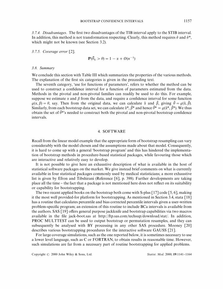
3.7.4. Disadvantages. The "rst two disadvantages of the TIB interval apply to the STIB interval.In addition, this method is not transformation respecting. Clearly, this method requires p( and p( *,which might not be known (see Section 3.2).


P(hIU'h)"1!a#O(n~1)

3.8. Summary

We conclude this section with Table III which summarizes the properties of the various methods.The explanation of the "rst six categories is given in the preceeding text.

The seventh category, &use for functions of parameters', refers to whether the method can beused to construct a con"dence interval for a function of parameters estimated from the data.Methods in the pivotal and non-pivotal families can readily be used to do this. For example,suppose we estimate a and b from the data, and require a con"dence interval for some functiong(a, b)"h, say. Then from the original data, we can calculate a( and bK , giving hK "g (a( , bK ).Similarly, from each bootstrap data set, we can calculate a( *, bK * and hence hK *"g (a( *, bK *). We thusobtain the set of hK *'s needed to construct both the pivotal and non-pivotal bootstrap con"denceintervals.

4. SOFTWARE

Recall from the linear model example that the appropriate form of bootstrap resampling can varyconsiderably with the model chosen and the assumptions made about that model. Consequently,it is hard to come up with a general &bootstrap program' and this has hindered the implementa-tion of bootstrap methods in procedure-based statistical packages, while favouring those whichare interactive and relatively easy to develop.

It is not possible to give here an exhaustive description of what is available in the host ofstatistical software packages on the market. We give instead brief comments on what is currentlyavailable in four statistical packages commonly used by medical statisticians; a more exhaustivelist is given by Efron and Tibshirani (Reference [6], p. 398). Further developments are takingplace all the time } the fact that a package is not mentioned here does not re#ect on its suitabilityor capability for bootstrapping.

The two recent applied books on the bootstrap both come with S-plus [17] code [5, 6], makingit the most well provided-for platform for bootstrapping. As mentioned in Section 3.4, stata [18]has a routine that calculates percentile and bias corrected percentile intervals given a user-writtenproblem-speci"c program; an extension of this routine to include BCa intervals is available fromthe authors. SAS [19] o!ers general purpose jackknife and bootstrap capabilities via two macrosavailable in the "le jack-boot.sas at http://ftp.sas.com/techsup/download/stat/. In addition,PROC MULTTEST can be used to output bootstrap or permutation resamples, and they cansubsequently be analysed with BY processing in any other SAS procedure. Mooney [20]describes various bootstrapping procedures for the interactive software GAUSS [21].

For large coverage simulations, such as the one reported below, it is sometimes necessary to usea lower level language, such as C or FORTRAN, to obtain results in reasonable time. However,such simulations are far from a necessary part of routine bootstrapping for applied problems.



Tab

leII

I.Sum

mar

yof

pro

per

ties

ofboot

stra

pco

n"den

cein

terv

alm

ethods

.F

or

furt

her

det

ails

on

the

cate

gories

,se

eSec

tion

3.8.

Met

hod

Theo

retica

lT

ransfor

mat

ion

Use

with

Use

with

p(,p(*

Anal

ytic

const

ant

Use

for

cove

rage

resp

ecting

par

amet

ric

non-

par

amet

ric

required

orva

rian

cest

abiliz

ing

funct

ions

of

erro

rsim

ulat

ion

sim

ula

tion

tran

form

atio

nre

quired

par

amet

ers

Non-S

tuden

tize

dpiv

ota

lO

(n~

1@2)

]@

@]

]@

Boot

stra

p-t

O(n

~1)

]@

@@

@@

Per

centile

O(n

~1@2)

@@

@]

]@

BC

per

centile

O(n

~1@2)

@@

@]

]@

BC

ape

rcen

tile

O(n

~1)

@@

@]

@@

Tes

t-in

vers

ion

O(n

~1@2)

@@

]]

]]

Studen

tize

dte

st-inve

rsio

nO

(n~

1)]

@]

@]

]



Table IV. Number of times, out of 10 000 replications, that equitailed 99 percent con"dence intervals constructed for the mean of an inverse exponentialdistribution, based on a sample of size 20 from the distribution, fail to includethe true parameter value, 1. Figures in parenthesis next to the interval coverage

are standard errors based on the binomial distribution.

Method Interval Mean length (SE)above 1 below 1

Expected 50 50 1.333Theoretical 45 (7) 52 (7) 1.332 (0.003)Non-Studentized pivotal 0 (0) 530 (22) 1.157 (0.003)Bootstrap-t 48 (7) 47 (7) 1.347 (0.003)Percentile 1 (1) 215 (14) 1.157 (0.003)BC percentile 5 (2) 169 (13) 1.178 (0.003)BCa percentile 50 (7) 56 (7) 1.330 (0.003)Test-inversion 46 (7) 50 (7) 1.351 (0.003)

5. SIMULATIONS STUDY: EXPONENTIAL DISTRIBUTION

We present the results of a simulation study comparing the simulation based methods describedso far applied to the problem of estimating a con"dence interval for the mean of an inverseexponential distribution, with density function

fX(x)"(1/j) exp(!x/j), j'0

based on a small sample from the distribution.Table IV gives results for the bootstrap methods and the test-inversion method. The

program repeatedly simulated an &observed' sample of size 20 from the inverse exponen-tial distribution with mean 1 and constructed intervals for the mean based on thatsample. For each &observed' sample from the inverse exponential distribution all thebootstrap intervals were constructed using the same set of B simulated observations.The TIB interval (which coincides with the STIB interval in this example) was estimatedusing the Robbins}Monro algorithm [16]. The Robbins}Monro search used B/2simulated observations in the search for each interval endpoint, making a total of B,which is equivalent to the number used to estimate the bootstrap intervals. The value ofB was 3999. Standard errors, calculated using the binomial distribution, are given inparentheses.

Table IV shows that the most reliable methods for estimating equitailed con"dence intervalsfor the mean of the inverse exponential distribution are the bootstrap-t and the test-inversionmethod (both happen to have theoretical coverage error zero in this example). The bias correctedand accelerated (BCa) percentile method cannot be relied on as the nominal coverage increasesand the sample size decreases. For example, with a sample size of "ve, the BCa interval was below1 a total of 180 times, while the test-inversion and bootstrap-t intervals remained below 1 50}60times, as expected.



Figure 4. Guide to choosing a bootstrap con"dence interval method when usingnon-parametric simulation.

Figure 5. Guide to choosing a bootstrap con"dence interval method when using parametric simulation, orsimulating in a regression framework, as described in Section 2.3.

6. GUIDE TO CHOOSING A METHOD

The advantages and disadvantages of the above methods, together with our experience onvarious examples, are summarized by Figures 4 and 5. These are decision trees, which can be usedto select an appropriate method for a particular application when using non-parametric andparametric resampling, respectively. Where the box at the end of the decision tree has more thantwo methods, we slightly prefer the "rst method given. However, as a check, both methods can beused and the resulting intervals compared.



7. WORKED EXAMPLE: REMISSION TIMES FROM ACUTE MYELOGENOUSLEUKAEMIA

We now continue with our motivating example 1.1. Recall that we "tted a proportional hazardsmodel to the data. This gave an estimate bK "0.924 of the treatment e!ect b and a standard errorp("0.512. A standard normal approximation con"dence interval for b is therefore bK $1.96]0.512, which yields (!0.080, 1.928). We wish to con"rm the accuracy of this interval using thebootstrap.

Depending on the statistic of interest, there are a variety of possible bootstrap samplingschemes for survival data (Davison and Hinkley, Reference [5], Chapter 7; Veraverbeke [22]).For simplicity, we consider only non-parametric (that is, case resampling) bootstrapping here.The non-parametric resampling proceeds as described in Section 2.1.

We sample with replacement from the set of 23 triples (ti, c

i, x

i) (representing the remission

time, a binary variable indicating censoring and a binary variable indicating treatment) to obtaina bootstrap data set of 23 triples. We then re"t the proportional hazards model to this data toobtain a bootstrap estimate bK *.

The procedure in the previous paragraph was repeated 1999 times. Examination of the resultsshowed that one of the bK *'s was over 20 times greater than the largest of the rest of the bK *'s. This isan example of a problem that occurs from time to time in bootstrap simulation, when anextremely unusual data set is generated. For example, in non-parametric sampling, a bootstrapdata set might consist of many copies of the same observation, and it might be impossible to "tthe statistical model to such a data set.

Such an extreme data set would have little impact on the bootstrap con"dence intervalif it were possible to construct the complete set of every possible bootstrap data set andcalculate the con"dence interval from this. However, this is not possible in practice. Inorder to avoid the chance occurrence of an extreme data set unduly in#uencing thebootstrap con"dence interval, we therefore advocate discarding such extreme data sets.Of course, if it is impossible to "t the statistical model to more than a few per cent of bootstrapdata sets, then, since such data sets can no longer be viewed as extreme data sets withinthe complete set of bootstrap data sets, this probably indicates that the statistical model isinappropriate.

In this case, we discarded the extreme data set, to avoid problems with the numerical routinesused to calculate the variance stabilized bootstrap-t interval.

A Q-Q plot of the 1998 remaining (bK *!bK )'s is shown in the upper left panel of Figure 6. Itappears to be slightly overdispersed relative to the normal distribution. This overdispersion is stillpresent in the upper tail of the distribution of (bK *!bK )/p( *, shown in the lower left panel ofFigure 6. Moreover, as the top right panel of Figure 6 shows, there is a strong relationshipbetween the value of bK * and its standard error p( *. With this information in mind, we now refer toFigures 4 and 5 to choose an appropriate method.

Since we carried out non-parametric simulation, Figure 4 is appropriate. Starting at top, p( andp( * are available from the information matrix of the proportional hazards model "tted to theoriginal and bootstrap data sets, respectively. Next, the top right panel of Figure 6 shows there isa strong correlation between the value of bK * and its standard error p( *. We are thus led to thevariance stabilized bootstrap-t or, as an alternative, the BCa interval.

These intervals are the last two entries in Table V, and they agree well. The results for variousother methods are also given, for comparison. We conclude that there is not quite enough



Figure 6. Diagnostic plots for the bootstrap con"dence intervals for the AML data: top left panel, Q-Q plotof the distribution of bK *!bK ; bottom left panel, Q-Q plot of the distribution of (bK *!bK )/p( *; top right panel,

plot of p* against bK *!bK ; bottom right, jackknife-after-bootstrap plot } details in the text.

Table V. Ninety-"ve per cent bootstrap con"dence intervals fortreatment e!ect, b, obtained using various methods. The maximumlikelihood estimate of b, bK "0.916, with standard error, calculated

in the usual way from the information matrix, of 0.512.

Method 95% interval

Normal approx. (bK $1.96]SE bK ) (!0.088, 1.920)Non-Studentized pivotal (!0.335, 1.856)Bootstrap-t (!0.148, 1.883)Percentile (!0.0253, 2.166)BCa (!0.159, 2.011)Variance stabilized bootstrap-t (!0.170, 2.067)

evidence to reject the hypothesis that the two treatments are di!erent at the 5 per cent level, and inparticular that there is less evidence than suggested by the standard normal theory interval.

Before leaving this example, we perform a bootstrap diagnostic, to examine whether theconclusions depend heavily on any single observation. To do this we look at the estimateddistribution of bK *!bK when observations 1, 2, 2 , 23 are left out in turn. No additional



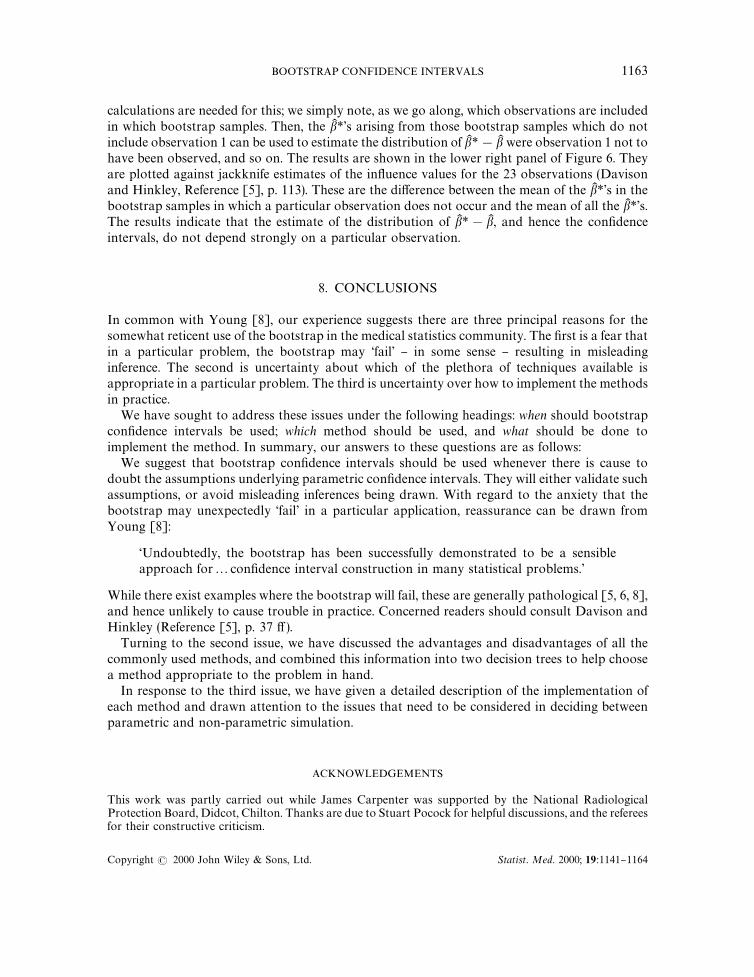
calculations are needed for this; we simply note, as we go along, which observations are includedin which bootstrap samples. Then, the bK *'s arising from those bootstrap samples which do notinclude observation 1 can be used to estimate the distribution of bK *!bK were observation 1 not tohave been observed, and so on. The results are shown in the lower right panel of Figure 6. Theyare plotted against jackknife estimates of the in#uence values for the 23 observations (Davisonand Hinkley, Reference [5], p. 113). These are the di!erence between the mean of the bK *'s in thebootstrap samples in which a particular observation does not occur and the mean of all the bK *'s.The results indicate that the estimate of the distribution of bK *!bK , and hence the con"denceintervals, do not depend strongly on a particular observation.

8. CONCLUSIONS

In common with Young [8], our experience suggests there are three principal reasons for thesomewhat reticent use of the bootstrap in the medical statistics community. The "rst is a fear thatin a particular problem, the bootstrap may &fail' } in some sense } resulting in misleadinginference. The second is uncertainty about which of the plethora of techniques available isappropriate in a particular problem. The third is uncertainty over how to implement the methodsin practice.

We have sought to address these issues under the following headings: when should bootstrapcon"dence intervals be used; which method should be used, and what should be done toimplement the method. In summary, our answers to these questions are as follows:

We suggest that bootstrap con"dence intervals should be used whenever there is cause todoubt the assumptions underlying parametric con"dence intervals. They will either validate suchassumptions, or avoid misleading inferences being drawn. With regard to the anxiety that thebootstrap may unexpectedly &fail' in a particular application, reassurance can be drawn fromYoung [8]:

&Undoubtedly, the bootstrap has been successfully demonstrated to be a sensibleapproach for2con"dence interval construction in many statistical problems.'

While there exist examples where the bootstrap will fail, these are generally pathological [5, 6, 8],and hence unlikely to cause trouble in practice. Concerned readers should consult Davison andHinkley (Reference [5], p. 37 ! ).

Turning to the second issue, we have discussed the advantages and disadvantages of all thecommonly used methods, and combined this information into two decision trees to help choosea method appropriate to the problem in hand.

In response to the third issue, we have given a detailed description of the implementation ofeach method and drawn attention to the issues that need to be considered in deciding betweenparametric and non-parametric simulation.

ACKNOWLEDGEMENTS

This work was partly carried out while James Carpenter was supported by the National RadiologicalProtection Board, Didcot, Chilton. Thanks are due to Stuart Pocock for helpful discussions, and the refereesfor their constructive criticism.



REFERENCES

1. Embury SH, Elias L, Heller PH, Hood CE, Greenberg PL, Schrier SL. Remission maintenance therapy in acutemyelogenous leukaemia.=estern Journal of Medicine 1977; 126:267}272.

2. Carpenter JR. Test-inversion bootstrap con"dence intervals. Journal of the Royal Statistical Society, Series B 1999;61:159}172.

3. LePage R, Billard L (eds). Exploring the ¸imits of Bootstrap. Wiley: New York, 1992.4. Armitage P, Berry G. Statistical Methods in Medical Research. Blackwell: Oxford, 1987.5. Davison AC, Hinkley DV. Bootstrap Methods and their Application. Cambridge University Press: Cambridge, 1997.6. Efron B, Tibshirani RJ. An Introduction to the Bootstrap. Chapman and Hall: London, 1993.7. Cox DR, Hinkley DV. ¹heoretical Statistics. Chapman and Hall: London, 1974.8. Young GA. Bootstrap * more than a stab in the dark? Statistical Science 1994; 9:382}415.9. Hall P. ¹he Bootstrap and Edgeworth Expansion. Springer-Verlag: London, 1992.

10. DiCiccio TJ, Efron B. Bootstrap con"dence intervals. Statistical Science 1996; 11:189}212.11. Efron B. ¹he Jackknife, the Bootstrap and other Resampling Plans. Society for Industrial and Applied Mathematics:

Philadelphia, 1982.12. Efron B. Better bootstrap con"dence intervals. Journal of the American Statistical Association 1987; 82:171}200.13. Efron B. More accurate con"dence intervals in exponential families. Biometrika 1992; 79:231}245.14. Rao CR. ¸inear Statistical Inference and its Applications. Wiley and Sons: London, 1973.15. Carpenter JR. Simulated con"dence regions for parameters in epidemiological model. D. Phil. thesis, Oxford

University, 1997.16. Buckland ST, Garthwaite PH. Estimating con"dence intervals by the Robbins}Monro search process. Journal of the

Royal Statistical Society, Series C 1990; 39:413}424.17. MathSoft, Inc., 101 Main Street, Cambridge, MA 02142-1521 USA.18. Stata Corporation, 702 University Drive East, College Station, Texas 77840 USA.19. SAS Institute Inc. SAS Campus Drive Cary, NC 27513, USA.20. Mooney C. Bootstrapping: A Non-parameteric Approach to Statistical Inference. SAGE: London, 1993.21. Aptech Systems Inc., Maple Valley, WA, USA.22. Veraverbeke N. Bootstrapping in survival analysis. South African Statistical Journal 1997; 31:217}258.23. Efron B. Nonparametric standard errors and con"dence intervals (with discussion). Canadian Journal of Statistics

1981; 9:139}172.24. Kabaila P. Some properties of pro"le bootstrap con"dence intervals. Australian Journal of Statistics 1993; 35:205}214.



Bootstrap confidence intervals: when, which, what? …saharon/Boot/10.1.1.133.8405.pdfSTATISTICS IN...

Documents

Transcript of Bootstrap confidence intervals: when, which, what? …saharon/Boot/10.1.1.133.8405.pdfSTATISTICS IN...