Session 3: Some Data Operations

The Swiss Credit Card Data: Bagging

The Stormer Viscometer Data: Non-linear Regression, Bootstrap Confidence

Intervals

Swiss Credit Card Data

• Main response: Does this customer own a credit card?

• Predictors: various personal details (age, sex, language, ...) and account use behaviour

• Problem: Build a predictor for credit card ownership

• Strategies:– Logistic regression with stepwise variable

selection, penalized by BIC– Trees– Trees with discrete bagging– Trees with smooth bagging

Split data into "train" and "test" sets

SwissCC <- read.csv("SwissCC.csv")

### set seed

set.seed(300424)

###

k <- nrow(SwissCC)

isp <- sample(k, floor(0.4*k))

CCTrain <- SwissCC[isp, ]

CCTest <- SwissCC[-isp, ]

require(ASOP)

Save(SwissCC, CCTrain, CCTest, isp)

Stepwise Logistic Regression

### try a logistic regression

CCLR <- glm(credit_card_owner ~ 1, binomial, CCTrain)

### construct an upper list as a formulam <- match("credit_card_owner", names(CCTrain))form <- as.formula(paste("~",

paste(names(CCTrain)[-m], collapse = "+")))

require(MASS)sCCLR <- stepAIC(CCLR,

scope = list(lower = ~1, upper = form), trace = FALSE, k = log(nrow(CCTrain)))

Trees

##### treesrequire(rpart)CCTM <- rpart(credit_card_owner ~ ., CCTrain)plotcp(CCTM) # other checks possibly...

### Constructing the formula explicitlym <- match("credit_card_owner", names(SwissCC))others <- names(SwissCC)[-m]plusGroup <- function(nam) if(length(nam) == 1) as.name(nam) else

call("+", Recall(nam[-length(nam)]), as.name(nam[length(nam)]))

form <- call("~", as.name("credit_card_owner"),

plusGroup(others))

Bagging

• Two versions, 'discrete' and 'bayesian' ('smooth')– Discrete bagging:

• Construct a forest of trees got from ordinary bootstrap samples of the training data

– Bayesian bootstrap bagging:• Construct a forest of trees got by randomly

weighting the entries of the training data, with Gamma(1,1) (i.e. exponential) weights.

• Predict the class for each tree in the forest• Declare the simple majority vote the predictor

#### bagged trees

baggedRPart <- function(object, style = c("discrete", "bayesian"), data = eval.parent(object$call$data), nbags = 100, seed = 130244) { style <- match.arg(style) set.seed(seed) k <- nrow(data) bag <- structure(list(), randomSeed = seed) switch(style, discrete = for(i in 1:nbags) bag[[i]] <- update(object,

data = data[sample(k, rep = TRUE), ]),

bayesian = for(i in 1:nbags) bag[[i]] <- update(object,

weights = rexp(k)) ) oldClass(bag) <- "baggedRPart" bag}

Notes• Would work with any model object that allows

updating with new data sets or new weights– Examples: nls(), tree(), glm(), ...

• A more general function would return an object with some information on the class of the primary object in the inheritance train

• e.g.oldClass(val) <- c("bagged", paste("bagged",

class(object), sep = "."))• The package 'ipred' has a more general bagging() function that constructs the initial object itself

Prediction from the forest of bags

predict.baggedRPart <- function(object, newdata, ...) {

preds <- lapply(object, predict, newdata, type = "class")

preds <- do.call("cbind", lapply(preds, as.character))

preds <- apply(preds, 1, function(x) {

tx <- table(x) names(tx)[which(tx == max(tx))[1]] }) names(preds) <- names(object) preds}

Notes

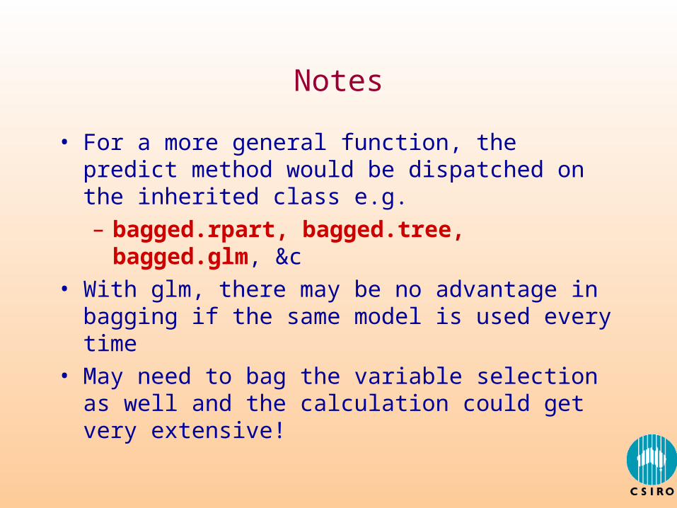
• For a more general function, the predict method would be dispatched on the inherited class e.g.– bagged.rpart, bagged.tree, bagged.glm, &c

• With glm, there may be no advantage in bagging if the same model is used every time

• May need to bag the variable selection as well and the calculation could get very extensive!

Recording the results and checking

############# some tests

bdCCTM <- baggedRPart(CCTM)

bbCCTM <- baggedRPart(CCTM, style = "b")

CCTest <- transform(CCTest,

psCCLR = ifelse(predict(sCCLR, CCTest,

type = "response") > 0.5, "yes", "no"),

pCCTM = predict(CCTM, CCTest, type = "class"),

pbdCCTM = predict(bdCCTM, CCTest),

pbbCCTM = predict(bbCCTM, CCTest))

Confusion, confusion, confusion ...### look at the confusion matrices

confusion <- function(f1, f2) { tab <- table(f1, f2) names(dimnames(tab)) <- c(deparse(substitute(f1)), deparse(substitute(f2))) oldClass(tab) <- "confusion" tab}

errorRate <- function(confusion) 1 - sum(diag(confusion))/sum(confusion)

print.confusion <- function(x, ...) { x <- unclass(x) NextMethod("print", x) cat("Error rate: ",

format(100*round(errorRate(x), 4)), "%\n") invisible(x)}

The final showdown

with(CCTest, {

print(confusion(credit_card_owner, psCCLR))

print(confusion(credit_card_owner, pCCTM))

print(confusion(credit_card_owner, pbdCCTM))

print(confusion(credit_card_owner, pbbCCTM))

invisible()

})

psCCLRcredit_card_owner no yes No 484 96 Yes 67 604Error rate: 13.03 % pCCTMcredit_card_owner No Yes No 455 125 Yes 45 626Error rate: 13.59 % pbdCCTMcredit_card_owner No Yes No 478 102 Yes 47 624Error rate: 11.91 % pbbCCTMcredit_card_owner No Yes No 478 102 Yes 51 620Error rate: 12.23 %

Comments

• Not a very convincing demonstration, but bagging usually does show some improvement

• With a continuous response, the predictions are averaged over the forest

• Bagging has been shown to benefit only models with substantial non-linearity, so will not work much on linear models, eg

• randomForest is a package that further develops the bagging idea

• gbm is a 'gradient boosting method' package that uses a more systematic approach.

Non-linear regression: self starting models

• Stormer data– Time = b * Viscosity/(Wt – g)

• 'b' and 'g' unknown parameters• initial values:

– Wt * Time = b * Viscosity + g * Time• statistically nonsense, but worth using as a

starting procedure

An initial look at the model

library(MASS)b <- coef(lm(Wt*Time ~ Viscosity + Time - 1, stormer))names(b) <- c("beta", "theta")b

beta theta 28.875541 2.843728

storm.1 <- nls(Time ~ beta*Viscosity/(Wt - theta),

stormer, start = b, trace = T)885.3645 : 28.875541 2.843728 825.1098 : 29.393464 2.233276 825.0514 : 29.401327 2.218226 825.0514 : 29.401257 2.218274

summary(storm.1)

Encapsulating it in a self-starter

storm.init <- function(mCall, data, LHS) {

v <- eval(mCall[["V"]], data) ## links below

w <- eval(mCall[["W"]], data) ## links below

t <- eval(LHS, data) ## links below

b <- lsfit(cbind(v, t), t * w, int = F)$coef

names(b) <- mCall[c("b", "t")]

b

}

NLSstormer <- selfStart( ~ b*V/(W-t), storm.init, c("b","t"))

Checking the procedure

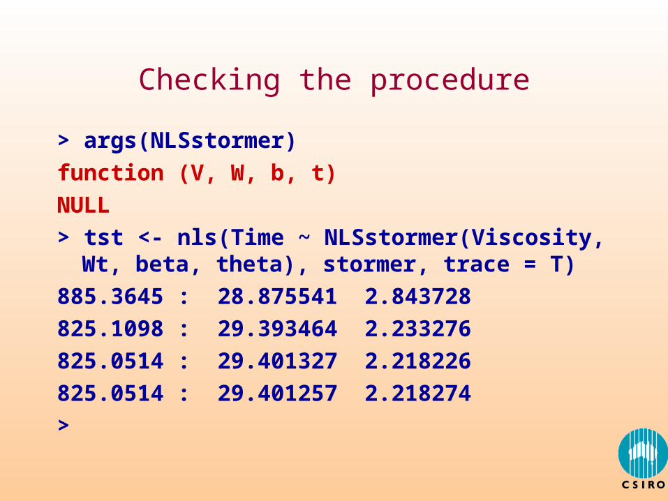
> args(NLSstormer)

function (V, W, b, t)

NULL

> tst <- nls(Time ~ NLSstormer(Viscosity, Wt, beta, theta), stormer, trace = T)

885.3645 : 28.875541 2.843728

825.1098 : 29.393464 2.233276

825.0514 : 29.401327 2.218226

825.0514 : 29.401257 2.218274

>

Confidence intervals

• Three strategies:– Normal theory: beta-hat +/- 2 sd.– Bootstrap re-sampling of the centred

residuals– Bayesian bootstrap weighting of the

observations• From the summary:Parameters:

Estimate Std. Error

beta 29.4013 0.9155

theta 2.2183 0.6655

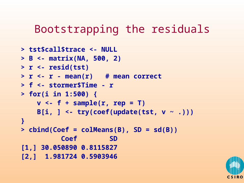
Bootstrapping the residuals

> tst$call$trace <- NULL> B <- matrix(NA, 500, 2)> r <- resid(tst)> r <- r - mean(r) # mean correct> f <- stormer$Time - r> for(i in 1:500) { v <- f + sample(r, rep = T) B[i, ] <- try(coef(update(tst, v ~ .))) }> cbind(Coef = colMeans(B), SD = sd(B)) Coef SD[1,] 30.050890 0.8115827[2,] 1.981724 0.5903946

Smooth bootstrap re-sampling

> n <- nrow(stormer)

> B <- matrix(NA, 1000, 2)

> for(i in 1:1000)

B[i, ] <-

try(coef(update(tst,

weights = rexp(n))))

> cbind(Coef = colMeans(B), SD = sd(B))

Coef SD

[1,] 29.367936 0.5709821

[2,] 2.252755 0.5811193

Final remarks

• Bootstrap methods appear to give reasonable standard errors for the non-linear parameter, but not the linear

• The model may not in fact 'fit' very well• An alternative to for-loops would be to use

unrolled loops in a batch run – details on request...!