BOLTED CONNECTIONS IN S - COnnecting … · This thesis aims to investigate the characteristics and...
93
Faculty of Engineering, Health, Science and the Environment School of Engineering and Information Technology BOLTED CONNECTIONS IN STRUCTURAL STEELWORK Author: Cielo Marie Alvaran s213623 A thesis submitted in partial fulfilment of the requirement for the degree of Bachelor of Engineering Co-Op Thesis Supervisor: Professor David Lilley Professor of Structural Engineering at Charles Darwin University June 2014
Transcript of BOLTED CONNECTIONS IN S - COnnecting … · This thesis aims to investigate the characteristics and...

Faculty of Engineering, Health, Science and the Environment
School of Engineering and Information Technology
BOLTED CONNECTIONS IN
STRUCTURAL STEELWORK
Author:
Cielo Marie Alvaran
s213623
A thesis submitted in partial fulfilment of the requirement for the degree of
Bachelor of Engineering Co-Op
Thesis Supervisor:
Professor David Lilley
Professor of Structural Engineering at Charles Darwin University
June 2014

Abstract:
This thesis aims to investigate the characteristics and structural properties of bolted
connections in steel structures with the main focus on the design adequacy and failure
mechanisms of high-strength friction-grip (HSFG) bolted connections.
As a case study, the bolted connections on the Mary River Bridge along Arnhem Highway in
the Northern Territory have been investigated. The composite highway bridge is composed of
reinforced concrete deck over five simply supported spans of structural steelwork. The
structural steelwork includes five main UB girders connected to diaphragms and horizontal
bracings by HSFG bolted connections. Initial inspection of the bridge found that a number of
bolts were loosened, missing or had already fractured and most were heavily corroded.
Remedial works in which the original bolted connections have been replaced and the new
ones ensured to be installed at the correct tension have been recently completed.
The structural and environmental factors that may have contributed to the eventual failure of
the bolts have been investigated. The design adequacy of the bolted connections compared to
the externally applied loads on the bridge superstructure was checked in accordance with
current standards: AS5100 and AS4100. The failure mechanisms of the fractured bolts were
investigated. The residual loads on the original bolts have been identified through slip testing
on both the original bolts and new HSFG bolts in double shear configuration. The fractured
bolts were analysed through optical and scanned electron microscopy. The design fatigue life
of the bolts were identified through fatigue testing of the M16 bolts in double shear
configuration and the M22 bolts subjected to cyclic tensile load. The difference of the rate of
corrosion of the bolts with and without the zinc plate corrosion protection was also identified.
It was found that the main factors the contributed to the failure of the bolted connections at
the Mary River Bridge include overstressing of the bolts, the fluctuating loads, the eventual
abrasion and wear of the corrosive protection and the corrosive environment it was subjected
to. The failure mechanisms of the fractured bolts were mainly due to corrosion and fretting
fatigue. Similarly, the bolts subjected to tension, have failed due to self-loosening over time.
Keywords:
highway bridge, HSFG bolts, modes of failure

ACKNOWLEDGEMENTS
I would like to express my gratitude for the constant guidance and unwavering patience of
my supervisor Prof. David Lilley.
I’m also grateful to Richard Underhill, Krishnan Kannoorpatti and Margarita Vargas for their
feedbacks and guidance.
Undertaking this thesis has been challenging and completing this report would not have been
possible without the guidance of these people, so again, thank you.

LIST OF TABLES
Table 1: UB members dimensions (Polsteel, 2012) ................................................................... 5
Table 2: Summary of Bolt types and categories (GAA) .......................................................... 11
Table 3: Corrosion rate of steel and zinc in C3 zones (GAA, 2012) ........................................ 14
Table 4: Permissible Loads on the Mary River Bridge according to the Report on Bridge
Load Capacities (1979) ............................................................................................................. 28
Table 5: Vertical and Horizontal Loads on the Bridge Superstructure over one span ............. 33
Table 6: Vickers Hardness Results ........................................................................................... 40
Table 7: Slip loads of Old and New bolts ................................................................................. 45
Table 8: Fatigue Testing Parameters ........................................................................................ 48
Table 9: Bolt Specimens Properties .......................................................................................... 50
Table 10: Total Surface Area exposed to corrosive media ....................................................... 50
Table 11: Weight loss after corrosion by immersion testing .................................................... 51
Table 12: Design Shear and Tension - Strength Limit State (Blacks Fasteners) ..................... 60
Table 13: Design Shear - Serviceability Limit State (Blacks Fasteners) ................................. 60

LIST OF FIGURES
Figure 1: Bridge Cross Section (DoW, 1968) ............................................................................ 5
Figure 2: Concrete Slab as top flange ......................................................................................... 8
Figure 3: Grillage System for a Two-Span Bridge (SCI, 2012) ................................................. 9
Figure 4: (a) Bearing and shear and (b) friction grip on a bolted lap joint (Gorenc, 2012) ..... 10
Figure 5: ASSHTO and Eurocode S-N curves (NHCRP, 2012) .............................................. 13
Figure 6: Life to First Maintenance of Hot Dipped Galvanized Steel (GAA, 2012) ............... 14
Figure 7: Percentage Error and Relative Cost in Bolt Installation (Fernando, 2001) .............. 15
Figure 8: Typical failure points of a bolt: (a) head fillet, (b) thread runout, ............................ 16
Figure 9: Joint Face Angularity (Bolt Science Limited, 2013) ................................................ 16
Figure 10: Major Steps in Conducting a Failure Analysis (Davidson, 1999) .......................... 18
Figure 11: Diamond Indenter for Hardness Test (ibid., p112) ................................................. 20
Figure 12: FHWA Transverse Wind Load Reactions at Pier bearings from Wind on
Superstructure ........................................................................................................................... 30
Figure 13: A160 Axle Load (SA, 2004) ................................................................................... 30
Figure 14: S1600 Stationary Traffic Load (SA, 2004) ............................................................. 31
Figure 15: M1600 Moving Traffic Load (SA, 2004) ............................................................... 31
Figure 16: M1600 loading position causing maximum bending moment over one span ......... 31
Figure 17: Horizontal Loads on a Bridge Span (in Plan View) ................................................ 32
Figure 18: Vertical Loads over a beam .................................................................................... 33
Figure 19: Resultant Shear Forces(maximum of 916kN at LHS support) ............................... 34
Figure 20: Bending Moment Diagram (maximum of 5127 kNm) ........................................... 34
Figure 21: Grillage Model of Bridge Span Superstructure ....................................................... 35
Figure 22: EDS Spectrum of Sample (prior to acid pickling) .................................................. 41
Figure 23: Macrographs of Fractured Surfaces for Sample A and Sample B .......................... 42
Figure 24: Shear Slip Testing Results ...................................................................................... 45
Figure 25: New M16 bolts loaded over slip critical load (Graph generated by software used
by the machine) ........................................................................................................................ 46
Figure 26: Old 5/8” bolts loaded over slip critical load (graph generated by use of raw data
from testing) ............................................................................................................................. 46
Figure 27: M16 and 5/8" bolts loaded over design slip capacity ............................................. 46
Figure 28: One Cycle of Load Applied .................................................................................... 48

LIST OF ILLUSTRATIONS
Illustration 1: Mary River Bridge (Bennett, 2013) ..................................................................... 5
Illustration 2: Mary River Bridge Telemetered Gauging Station (NRETA, 2007) .................... 5
Illustration 3: Mary River Bridge from the end abutment .......................................................... 6
Illustration 4: Inverted V brace at abutment ............................................................................... 6
Illustration 5: UB Diaphragm section ......................................................................................... 6
Illustration 6: EM Photomicrographs of Fracture Surfaces Exhibiting (a) Dimpled Fracture,
(b) Brittle Transgranular Fracture, (c) Intergranular Fracture, and (d) Fatigue Striations
(Shamsudin, 2011) .................................................................................................................... 19
Illustration 7: Test Fixtures for Slip and Cyclic loading (from left to right: M16 double shear
plates, M22 double shear plates, M16 2 bolts in tensile T-plates and M22 in tensile L-plates)24
Illustration 8: Set-up for Tensile Testing of M22 bolts ........................................................... 24
Illustration 9: Fractured 5/8" Bolt Samples A and B from bridge diaphragms ........................ 38
Illustration 10: Heavily Corroded 7/8" Nuts............................................................................. 38
Illustration 11: SEM micrograph at the outer surface .............................................................. 42
Illustration 12: SEM micrograph on fracture surface showing “indentations” .................... 42
Illustration 13: Surface Fractograph After Acid Pickling along a surface crack ...................... 43
Illustration 14: Surface Fractograph at Final Fracture .............................................................. 43
Illustration 15: Surface Fractograph at 500x Magnification .................................................... 43
Illustration 16: Surface Fractograph at 1000x Magnification .................................................. 43
Illustration 17: Surface Fractograph at 2000x Magnification .................................................. 44
Illustration 18: Bolt Fracture Surface ....................................................................................... 44
Illustration 19: Fatigue Cracks at the Bolt Fracture Surface .................................................... 44
Illustration 20: Slip Load Testing Setup ................................................................................... 45
Illustration 21: M22 tensile testing set-up ................................................................................ 47
Illustration 22: Corrosion by immersion set-up ........................................................................ 49

TABLE OF CONTENTS
1. Introduction .................................................................................................................................... 1
1.1. Background ............................................................................................................................ 1
1.2. Scope and Approach............................................................................................................... 2
2. Literature Review ........................................................................................................................... 4
2.1. The Mary River Bridge .......................................................................................................... 4
2.2. Bridge Loading ....................................................................................................................... 7
2.2.1. Bridge Design Loads ...................................................................................................... 7
2.2.2. Analysis of Composite Concrete and Steel Girder Bridges ........................................... 7
2.3. Bolted Connections ................................................................................................................ 9
2.3.1. Bolt Types and Properties .............................................................................................. 9
2.3.2. Design of High Strength Friction Grip (HSFG) Bolts.................................................. 11
2.4. Mechanical Modes of Bolt Failure ....................................................................................... 14
2.4.1. Overstressing ................................................................................................................ 14
2.4.2. Cyclic Loading ............................................................................................................. 15
2.4.3. Corrosion ...................................................................................................................... 16
2.5. Metal Failure Analysis ......................................................................................................... 17
3. Methodology of Analysis and Testing ......................................................................................... 22
3.1. Investigation of Design Adequacy of the Bridge Connections ............................................ 22
3.2. Failure Analysis of the Bolts Taken from the Bridge........................................................... 23
3.3. Methodology of Mechanical Testings Conducted ................................................................ 24
3.4. Corrosion by Immersion ....................................................................................................... 25
4. Investigation on Design Adequacy of Bolted Connections on Mary River Bridge ..................... 27
4.1. Mary River Bridge Loads ..................................................................................................... 27
4.1.1. Original Design Loads ................................................................................................. 27
4.1.2. Design Loads based on Current Standards ................................................................... 28
4.2. Bolted Connections at the Mary River Bridge ..................................................................... 34
5. Bolt Failure Analysis Results and Discussion .............................................................................. 37
5.1. Inspection of Conditions of Bolted Connections at the Mary River Bridge ........................ 37
5.2. Microstructure ...................................................................................................................... 39
5.3. Residual Loads ..................................................................................................................... 45
5.4. Fatigue Testing ..................................................................................................................... 48
5.5. Corrosion Testing ................................................................................................................. 49
6. Summary, Conclusion and Recommendations ............................................................................. 52
6.1. Summary of Findings ........................................................................................................... 52

6.1.1. Design Adequacy of the HSFG joints .......................................................................... 52
6.1.2. Bolt Analysis and Testing ............................................................................................ 52
6.1.3. Failure Mechanism of the HSFG bolts At Mary River Bridge .................................... 53
6.2. Conclusion ............................................................................................................................ 54
6.3. Recommendations ................................................................................................................ 55
6.3.1. Maintenance of Steel Structures ................................................................................... 55
6.3.2. Thesis Improvement ..................................................................................................... 55
6.3.3. Further Studies ............................................................................................................. 56
References ............................................................................................................................................ 57
Appendices ........................................................................................................................................... 60
Appendix A. Load Capacity of M16 and M22 bolts .................................................................. 60
Appendix B. Bridge Loading Analysis ...................................................................................... 62
1. Calculations of Loads on the Superstructure ........................................................................ 62
2. Microstran Analysis Reports ................................................................................................ 67
Appendix C. Specified Properties of 8.8/TF bolts ..................................................................... 76
Appendix D. Bolts, Nuts and Washers Inventory ...................................................................... 77
Appendix E. Equipment Used for Sample Preparation, Bolt Analysis and Bolt Testing .......... 79
Appendix F. Vickers Hardness Testing ..................................................................................... 80
Appendix G. Images from Optical and Scanned Electron Microscopy ..................................... 82
Appendix H. Mechanical Testings ............................................................................................. 83
1. One Set of Slip Load Graph from the Slip Testing Experiments ......................................... 83
2. Fatigue Testing Experimental Design .................................................................................. 83

1
CHAPTER 1
1. INTRODUCTION
1.1. BACKGROUND
Connections are essential members of a structure allowing the applied load to be transferred
effectively between the structural members and transmitted to the ground. For a steel
structure, these loads include the dead loads due to structural self-weight and all the external
loads to which the structure is subjected to. In bridges, these forces include the road traffic
loads, wind loads, forces due to water flow and many others as specified in relevant clauses
of the bridge design standards: AS5100 (SA, 2004). As the load applied on the system varies,
the structure must be capable of resisting the loading condition causing the most adverse
effect. Members of a structural steel framework are connected either by welding, riveting or
bolting. These connections must hence, be capable of transferring the design strength and
serviceability loads. As bridges experience cyclic loading conditions, the type of bolted
connections most commonly used for its superstructure are the high-strength friction-grip
(HSFG) bolts.
The design of bolted connections and the type of bolts used, vary depending on the loads the
structure itself is subjected to. Structural steel bolts are categorised according to grades and
methods of installation. Categories of bolts in steel construction include commercial bolts,
high-strength structural bolts and precision bolts (Gorenc et al, 2012, p206). Depending on
the modes of force transfer in which they are subjected to and allowance in slippage of
surfaces, the bolts are then further categorised as either bearing or friction type (ibid, p208).
The appropriate bolt type must be chosen in the design of the connection depending on the
nature and combination of loads. When the bolts are either in shear, in tension or loaded in
both shear and tension, the connections must be designed to conform to the strength and
serviceability limit states as specified in relevant clauses of AS4100 (Standards Australia,
1998).
As parts of the structure, connections are also subjected to the effects of environmental
conditions and repetitive loadings, if any. If exposed to oxygen and water, connections may
suffer from wet corrosion, in which, the rusting may occur rapidly (Ashby & Jones, 2005).

2
Due to fluctuating loads on a structure, its connections may hence also be subjected to fatigue
loading.
In AS4100, HSFG bolts of grade 8.8 are referred to as Grade8.8/TF bolts as As HSFG bolts,
specifically that of grade 8.8, otherwise referred to as Grade8.8/TF bolts in AS4100, is the
most commonly used bolt type connection in general structural steelwork (Barber, 1992), the
main focus of this thesis is investigating the properties both structural and environmental
affecting the life span of this type of bolted connection.
Mary River Bridge is a composite steel girders and concrete deck bridge of over 100m length
located along Arnhem Highway in the Northern Territory. The bridge has recently undergone
rehabilitation works in which the HSFG bolted connections throughout the superstructure
have been replaced. From inspection conducted by the Department of Infrastructure (DoI), it
was found that the majority of the bolts (from both diameters: 16mm and 22mm) in the
structure were either rusted or missing. This has then led to the question at hand of whether
or not these connections have failed prematurely, or before their design life span, and if so,
what may have caused said failures.
1.2. SCOPE AND APPROACH
The aim of this thesis is to investigate the characteristics and structural properties of bolted
connections in steel structures, specifically that of HSFG. This has been achieved through the
completion of the following tasks:
1. Intensive review of related literature of the following topics:
Types and designs of bolted connections on steel structures, including High Strength
Friction Grip (HSFG) bolts and other more conventional bolted connections, and
comparison of their material characteristics and structural properties,
Causes of failure on bolted connections on steel structures such as environmental
factors causing corrosion and crack propagation, and fatigue loading and thermal changes
on the structures causing yielding, loosening or unthreading of the bolts,
Metallurgical testing mechanisms and failure analysis,
Behaviour of bolted connections in response to application of dynamic loads on the
steel structure (such as fracture and loosening),
Standards for appropriate maintenance of bolted connections in structural steelwork.

3
2. Investigation of bolted connections on the Mary River Bridge along Arnhem Highway
through:
Determination and comparison of original design loads and loads causing most adverse
effects on the superstructure based on AS1170.0-2: Structural Design and AS5100.2:2004
Bridge Design Standard Design Loads and through finite element analysis,
Checking the adequacy of the design of the bolted connections in accordance with
AS4100.9: Design of Steel Structures: Bolted Connections.
3. Determination of causes of failure of the removed bolts from the existing connections on
the bridge and identification of material and structural properties of the existing bolted
connections, both from the removed original set of bolts and the new replacement bolts
through the following:
Metallographic examination of the original bolts through optical and scanned electron
microscopy,
Comparison of Vickers hardness of new and old bolts,
Slip testing as a measure of residual loads on the removed bolts compared to slip loads
of new HSFG bolts
Fatigue load testing to compare total service life of removed bolts to expected fatigue
life of bolts loaded to design loads
Corrosion by immersion testing of bolts with and without the zinc plating in different
corrosive media
4. From the research, analysis and testings as listed above, draw conclusions to answer the
following questions:
Have the bolts failed prematurely (or before expected end of service life)?
Are the bolted connections in Mary River Bridge adequate to resist the design loads
based on current standards?
What are the main causes of failure on the bolted connections of the bridge? And thus,
conclude on possible most common failure modes of HSFG bolts in structural steelwork.

4
CHAPTER 2
2. LITERATURE REVIEW
This chapter consists of the review of literature related to the main components of this thesis.
It includes the background research on the theories and similar past investigations related to
the thesis work found in various publications, as well as, a review of the design and history of
Mary River Bridge and its connections. This chapter includes a background on bridge loading
conditions and the design of its bolted connections, a study on various mechanical modes of
bolt failure and procedures for the analysis of metal failures and bolt testing. Brief summaries
and descriptions of some of the related publications are also included.
2.1. THE MARY RIVER BRIDGE
The Mary River Bridge is located at a section along Arnhem Highway with several
aggregates quarry sites nearby. Although, there is no nearby traffic counter in the area (the
closest of which is at the intersection of Arnhem Highway and Stuart Highway), a significant
percentage of the vehicles traversing over the bridge consists of loaded and unloaded trucks
from tipper trucks to multi-trailer transfer trucks.
The bridge is located within the Mary River Coastal Floodplain about 90km east of Darwin
(NRETAS, 2013). The floodplain is a large one but is poorly drained as instead of a direct
channel to the sea, the inflow diffuses over swamps and through tidal channels. The
floodplain thus experiences extended flooding over its wetland habitat areas. Over the years,
there have also been a major saltwater control program that have been implemented to
minimize saltwater intrusion in the floodplain (ibid.).
The three main sections of a bridge include the bridge deck, the superstructure (structural
steelwork or other) and the sub-structure (the headstocks and piers). The superstructure of
Mary River Bridge is made up of five equal spans of simply supported beams composed of a
concrete deck over five universal beam (UB) girders. The typical cross-section of the bridge
is illustrated in Figure 1 below The bridge was earlier constructed with three 762UB147
girders in 1968 and was then widened in 1972 with the addition of two 762UB197 girders of
the same web dimensions but higher flange width and hence, heavier sections (Department of

5
Works (DoW), 1968). Each beam was designed to span at 75ft centres (22.86m) and have a
total width of 24ft (7.315m).
Figure 1: Bridge Cross Section (DoW, 1968)
The section properties of the members are as tabulated below. As the UB members are bigger
than what is commercially available, the second moments of area about the X and the Y axes
were calculated.
Table 1: UB members dimensions (Polsteel, 2012)
Type Weight
[kg/m]
H: Web
height
[mm]
D:
Width
[mm]
d: Web
thickness
[mm]
h: Flange
thickness
[mm]
IX-area [mm4] IY-area [mm
4]
(H3d)/12 + 2* [(h3D)/12
+ h*D(H+h)2/4 ] (d3H/)12 + 2(D3h/12 )
762 x 267 UB
147
147 719 265.2 12.8 17.5 1.2897E+09 5.4401E+07
762 x 267 UB
197
197 719 268 15.6 25.4 1.9170E+09 8.1487E+07
The following figures are photographs of Mary River Bridge.
Illustration 1: Mary River Bridge (Bennett,
2013)
Illustration 2: Mary River Bridge Telemetered
Gauging Station (NRETA, 2007)
The second, third and fourth piers of the bridge can be seen in Illustration 1, where the pier in
which the river height gauge is adjacent to is the second pier along Arnhem Highway in the
outbound direction (also shown in Illustration 2).

6
Illustration 3: Mary River Bridge from the end abutment
The photograph in
Illustration 3 was taken from the end abutment of the bridge. It shows piers 3 and 4 and spans
4 and 5 of the bridge.
Illustration 4: Inverted V brace at abutment
Illustration 5: UB Diaphragm section
The figures below show the typical detail of the diaphragms and braces of the bridge. The
brace system (Illustration 4), positioned on each pier, is composed of sections similar to those
used in the girder. The diaphragms are located at the mid-span between each pier. In
Illustration 5, the bolt groups on the left are not aligned with those on the right as this view
shows the new beam at the left (from the 1972 widening) and the old beam (1968) at the
right. The horizontally oriented bolts at the diaphragms and the bracings are 5/8” in diameter
while the vertical bolts at the headstock and at the underside of the diaphragm-to-girder
connections are 7/8” diameter bolts. As these bolts are in imperial sizes, the replacement
bolts, as well as the bolts used for the experiments, were the M16 and M22 equivalent.

7
2.2. BRIDGE LOADING
2.2.1. BRIDGE DESIGN LOADS
The main bridge design loads covered in the book The Design of Modern Steel Bridges are
the dead loads, live loads, longitudinal forces on bridges, wind loading and thermal forces
(Chatterjee, 1991). Other possible sources of stresses on the superstructures were also
enlisted but have not been discussed in detail (ibid, p.74).
In AS5100.2: Design loads in bridge superstructures, the design loads include the following:
Dead Loads
Road Traffic Loads
Fatigue Load
Braking Forces
Collision Loads
Forces due to water flow and debris
Wind Load
Earthquake Load
(SA, 2004)
The bridge design live loadings from different guidelines, in different countries, vary not
only with the uniformly distributed loads and the axle loads, but also in terms of the number
of axles, axle width and the spacing between them. The American Association of State
Highway and Transportation Officials (AASHTO) specifications from the USA, BS5200-
1997 and Australia’s AS5100 stipulate different classes of vehicle loadings (Chatterjee, 1991;
SA, 2004).
According to Chatterjee (1991), the worst loading for 20m length bridge span is often caused
by more than three two-axled, medium-weight, compact vehicles rather than road-trains with
the heaviest loads and more axles (Chatterjee, 1991, p54). This implies that the heaviest loads
do not necessarily cause the most adverse effect and thus, in determining the design live
loads, analysis of the bridge response due to combination of various types of vehicles
traversing over the bridge must be conducted.
2.2.2. ANALYSIS OF COMPOSITE CONCRETE AND STEEL GIRDER BRIDGES
Composite construction of bridges has been practiced as an economical engineering
solution. In a composite steel and concrete bridge, the reinforced concrete slab is bonded to
the top of the steel girder and acts as part of its flange, as shown below (O’Connor, 1971).

8
In this configuration, the concrete, thus, effectively has two
main functions: (1) transmit the externally applied loads
(vehicle loads on deck) to the girder and (2) participate in
carrying the bending moments in the beam. By analysing the
concrete deck as effectively a section of the girder’s top
flange, the structural behaviour due to live loads can hence
be defined (ibid).
As the neutral axis of a composite section is at a higher depth on the UB, compared to when
UB is analysed alone, the stiffness and the section modulus of the composite section, are
hence also higher (Lawson & Wickens, 1992).
In concrete and steel-girder bridges, the structure is commonly made of a number of parallel
longitudinal members linked through a transverse system (ibid, p351).The load distribution in
this parallel girder system is complex and hence, special techniques are required in its
analysis. O’Connor (1971) states that for cases in which the main structure and the deck
beams are integral with a continuous deck slab, as is the case with the Mary River Bridge, the
load distribution can be analysed through two ways: (1) to subdivide the slab into areas
effectively acting as the upper flange on the steel girder beams or (2) subdivide the slabs such
that they are represented by additional transverse or longitudinal elements. The bridge is then
analysed as a grid system composed of longitudinal elements representing the parallel main
girders (topped with the concrete slab of the defined effective width) and transverse elements
representing the cross-girders, which in the case of the Mary River Bridge is the diaphragm at
mid-span and the braces on the piers.
The bridge analysis can be either a two-dimensional (2D) analysis or three-dimensional (3D).
The road traffic loads on the bridge can be analysed by simplifying the loading conditions
into two simple linear elastic models. The first beam being the cross-section in which the
steel girders act as pinned supports and the second beam is a simply supported beam
representing one span of the bridge between two piers. This method of analysis is both
simpler and quicker to carry out. However, it treats each beam as elastic and does not take
into account the transverse distribution of the loads over the concrete deck. The line beam
Figure 2: Concrete Slab as top
flange

9
also does not consider the effects of skew. This method is useful in preliminary design, but
may prove to be unrealistic in detail design (SCI, 2012).
In order to investigate the dynamic response of highway girder bridges, Huang and his
colleagues from the Department of Civil and Environmental Engineering in Florida (1995)
has modelled a girder bridge through the finite element method (FEM) as a grillage beam
system. In this system, the bridge is divided into grillage members, in both transverse and
longitudinal directions, with set node intervals. Shown in Figure 3 is an example of how a
two-span bridge is modelled as a grillage beam.
Figure 3: Grillage System for a Two-Span Bridge (SCI, 2012)
The grillage system can be applied through the use of Microstran Analysis and SAP2000
structural analysis software packages. In Microstran Analysis, the traffic loading condition
found to cause the most adverse effect can be found when analysed using simple linear
elastic models. This loading condition, together with the other design loads on the bridge
superstructure can then be applied in the grillage beam model of the bridge. A similar grillage
bridge can be modelled in SAP2000 wherein the traffic loads and the horizontal loads, such
as water flow and debris, can be modelled dynamically for a 3D analysis.
2.3. BOLTED CONNECTIONS
2.3.1. BOLT TYPES AND PROPERTIES
Bolts are categorised according to their property classes as either 4.6 commercial bolts, 8.8
high-strength structural bolts, or 8.8, 10.9 or 12.9 precision bolts (Gorenc, op cit). According
to Barber (1992) of The Steel Construction Institute (SCI), the most commonly used bolts in

10
structural connections are of grades 4.6 and 8.8. Each of these bolt connections must conform
to AS1111-1980 ISO Metric hexagon and commercial bolts and screws and AS/NZS1252-
1983: High-strength steel bolts with associated nuts and washers for structural engineering
respectively (Gorenc, op cit; SA, 1980; SA, 1983).
The three fundamental modes of force transfer in the design of individual bolts (in bolt
groups) are shear or bearing mode, friction mode and axial tension mode. The bolt axis for
the axial tension mode of force transfer is parallel to the applied external loads. This force
transfer is also applicable in combination with the other bolting categories as bolts are often
subjected to axial loads as well as the external forces being transferred (ibid). The bearing
and friction modes of force transfer are as illustrated in Figure 4.
Figure 4: (a) Bearing and shear and (b) friction grip on a bolted lap joint (Gorenc, 2012)
In shear or bearing mode, when the applied load acts perpendicular to the bolt axis, they are
transferred by shear and bearing on the connecting plies (GAA, 2011). In this mode, the
connection is allowed to slip until the bolts come in bearing contact (Gorenc, op cit). Similar
to the bearing mode, the loads in friction mode are transferred perpendicular to the bolt axis.
However, as the joints are designed to not allow for slippage under limit loads, the frictional
forces at the mating surfaces, as illustrated in Figure 1.b are able to resist external loads
(GAA & Gorenc, op cit). Both the 8.8/TB and 8.8/TF connections must be installed through
full tightening of the bolts (GAA, 2011). The following table, taken from a publication by the
Galvanizers Association of Australia, summarises the attributes of the different common bolt
types.

11
Table 2: Summary of Bolt types and categories (GAA)
Australian Steel Institute released publications by Hogan and Munter (2007) regarding the
bolting of steel structures containing tables summarising the attributes and design capacities
of different bolt types. The Steel Designer’s Handbook also includes such tables, as well as
discussion on the mechanisms of each joint type (Gorenc et al, 2012).
According to the Research Council on Structural Connections (RCSC), if the joint is
subjected to tensile fatigue loading, referring to the cyclic application of externally applied
service loads and prying force (if any), it must be designed to either be pre-tensioned or slip-
critical (2004).
Barber (1992) claimed that HSFG bolts of the general grade, as governed by the British
Standard (BS) 4395, amongst all the other bolt types, is the most commonly used type in
general structural steelwork. This thesis thus focuses on the design and properties of the
8.8/TF bolts.
2.3.2. DESIGN OF HIGH STRENGTH FRICTION GRIP (HSFG) BOLTS
AS4100-1998 defines friction-type connections as: “high-strength bolts tightened to induce a
specified minimum bolt tension so that the resultant clamping action transfers the design
shear forces at the serviceability limit state acting in the plane of the common contact
surfaces by the friction developed between the contact surfaces” (Standards Australia, 1998).

12
The design of high strength fully tensioned friction type joints differs from that of
conventional bolt connections as slip is required to be limited in the serviceability limit state
design (SA, 1998). Due to this, for 8.8/TF bolted connections, the strength and serviceability
limit states are assessed separately in accordance with AS4100 clauses 9.3.2 and 9.3.3
respectively. As shown in Appendix A, the calculations for the tensile load capacity of a
friction tightened bolt vary for both the strength limit state and the serviceability limit state or
strength limit state, the tensile capacity is determined similarly to bolts of different grade.
However, for the serviceability limit state, the slip factor is considered. The nominal
capacities of bolts in tension, shear and combined shear and tension must be calculated in
designing for both the strength and serviceability limit states, and the design loads
transmitted through the bolted connection must not exceed these values.
According to Barber (1992), general grade HSFG bolts, as covered by the British Standard
(BS) 4395, has the strength of 8.8 bolts given that the nominal diameter is less than 24mm,
which is the case in the bolts utilised in the Mary River Bridge.
Based on ASSHTO LRFD Bridge design, the bridge’s design life is the “period of time on
which the statistical derivation of transient loads is based is 75 years” whilst its service life is
the time it is expected to be in operation (Bartholomew, 2009, p12). The expected service life
of the bridge depends on the original designer while its actual service life actually varies
according to various factors such as the structure’s exposure conditions, quality of design,
materials used upon construction and maintenance periods (ibid, p13). The indicative value
for the design service life of bridges is 100 years (ibid, p14). NHCRP (12) has conducted a
research testing of steel components of bridges under fatigue loading conditions and
compared with the S-N curves according the ASSHTO and Eurocode standards as illustrated
in the figure below.

13
Figure 5: ASSHTO and Eurocode S-N curves (NHCRP, 2012)
In Australia, hot dipped galvanized (HDG) steel are commonly used commercially as its
performance in the Australian atmosphere is relatively predictable and that compared to other
cathodic protection such as electroplating, zinc-plating and paint, HDG provides the thickest
coating and longer life to first maintenance (LFM) (GAA, 2012 & AMA, 2009). Shown
below is a chart of approximated LFM of HDG steel. The bolted connections in Mary River
Bridge are classified into C3 (medium corrosivity) due to its atmospheric environmental
conditions and although the bridge itself is not directly adjacent to the coastal region, as
previously mentioned, the site has experienced salt water intrusion (GAA, 2012). From the
chart below, it could be seen, that the LFM of HDG steels in C3 classified zones within
Australia varies from 21 to 40 years depending on the thickness of the zinc corrosion
protection layer on the steel.

14
Figure 6: Life to First Maintenance of Hot Dipped Galvanized Steel (GAA, 2012)
GAA also developed a table based on ISO9223Corrosion of metals and alloys which
included the rate of corrosion of carbon steel and zinc in the different corrosivity category
(20112).The values for C3 classified zone are as tabulated below.
Table 3: Corrosion rate of steel and zinc in C3 zones (GAA, 2012)
Unit Carbon Steel Zinc
g/(m2a)
grams per square metre per year
200 to 400 5 to 15
µm/a
Recalculated in micrometres per year
25 to 50 0.7 to 2.1
2.4. MECHANICAL MODES OF BOLT FAILURE
Bolts generally fail due to one or a combination of overstress, fatigue and corrosion (Buda,
1994).
2.4.1. OVERSTRESSING
The bolts are said to be overstressed if they are subjected to loads which are higher than what
their capacities allow. This may be the case if the design of the bolted connections is
inadequate compared to the loads they are actually subjected to. Overstressing of the bolts
due to tensile loads may be caused by the following:
Preload or torque of the bolts during installation exceeds specified preload and hence,
reduces the bolt’s axial tensile strength.
Loads transmitted by the bolted connection exceed its ultimate tensile strength, which may
cause fracture on the bolt. (Buda, 1994, p85)

15
Another cause of failure is due to improper torque upon installation. In a Steel Construction
journal by Dr. Fernando (2001), he has stated that using torque as a measure of tension can
lead to high percentages of errors as shown in Figure 7.
Figure 7: Percentage Error and Relative Cost in Bolt Installation (Fernando, 2001)
2.4.2. CYCLIC LOADING
When a structure or any of its components is subjected to a cyclic tensile stress, fatigue
failure may occur (Taylor, 2003). This failure is characterised by an incremental propagation
of a fatigue crack on the material caused by each stress cycle (ibid, p25). Din and Ghazali
(2004) claims that currently, in designing steel structures subjected to fatigue loading, the
focus of the designer is normally on the main structural elements. This has been observed in a
number of publications, wherein the focus is in selecting structural members after
determining the design loads as the importance is on the internal stresses induced and the
displacements due to the externally applied loads and does not discuss connections
requirements in as much detail. They also claim that there is a presumption that fatigue
failure is not likely to happen and that bolt connections do not play a major role in resisting
such loads (ibid, p20). However, this has not been the case for structural collapses that have
occurred due to insufficient fatigue resistance on the bearings (ibid). The cyclic stresses, due
to alternating applied loads on the bolts, from the pre-load torque to the externally applied
service loads, may cause for failure below the bolt’s rated tensile strength (Buda, 1994).

16
Fatigue failure on bolts normally occurs on points where there is a change in the cross-
sectional area as shown in Figure 8. The joint face angularity, as indicated in Figure 9, caused
by uneven joint surfaces, also affects the fatigue life of a bolt.
Figure 8: Typical failure points of a bolt: (a)
head fillet, (b) thread runout,
(c) first thread to engage the nut (Hobson. 1997)
Figure 9: Joint Face Angularity (Bolt Science
Limited, 2013)
2.4.3. CORROSION
Corrosion is the process of material degradation due to exposure and hence, chemical or
electrochemical interaction with its environment. As metal reacts with its environment,
various types of metallic corrosion may occur (ACA, 2013). The metal may reach a point in
which it is no longer capable of functioning to its original design capacity due to corrosion in
which case, it is said that corrosion failure has occurred. Bolted connections are often coated
to prevent this; however, over time, the coating themselves corrode and hence, the outer layer
of the bolts themselves begin to corrode. Bolt failure due to corrosion is either in the form of
chemical decomposition, galvanic corrosion, corrosion fatigue or stress corrosion cracking
(Buda op cit).
Often, corrosion and fatigue both contribute to the eventual failure of a mechanical
component in failure modes including stress corrosion cracking (SCC), fretting corrosion and
corrosion fatigue. As previously mentioned, high strength bolts are used in high tensile load
applications. When these types of bolts are in the presence of corrosive agents, stress
corrosion cracking may occur (ibid). The two factors determining the rate in which the
corrosion assists crack propagation are the stress on the bolt and the fracture toughness of the
material (Buda, 1994). Fretting corrosion, on the other hand, occurs when the contact
surfaces between materials subjected to repetitive motion cause abrasion and wear of the
material’s surface. In terms of bolts, fretting corrosion would be observed on the bolt shank

17
as the motion of the plates cause abrasion and wear on the bolt due to the vibration as effect
of externally applied fluctuating loads. The abrasion on the bolt threads essentially remove
the corrosion protective layer on the bolt allowing for accelerated corrosion attack to occur.
The causes of bolt failure are not limited to the earlier discussed ones. Determining the
causes of bolt failure will thus enable the engineers, in charge of the design phase,
maintenance and quality assurance, to take proper actions in preventing the same type of
failures from occurring.
2.5. METAL FAILURE ANALYSIS
ASTM’s Standard Guide for Corrosion-Related Failure Analysis is a guideline intending to
assist in an analysis wherein corrosion is a possible causative factor for failure of the material
(2013). The standard discusses the steps that may help an investigator in identifying relevant
corrosion information contributing to eventual failure. These steps include organising the
analysis, examination of failure site conditions, observation of operating conditions at time of
failure, records of historical information when available, careful sampling, evaluation of
samples and failure assessment (ASTM International, 2013).
The online article entitled The Consequences of Bolt Failures have several examples of bolt
failures that have been involved in what the author called “serious losses” referring to both
the structural and economic damages (Roberts, 2013). Photographs of failed bolts,
examination of the failure surface and description of their primary cause of failure have been
included. Davidson published a paper on failure analysis from a series of case studies of bolt
connection failures (1999). The procedure generally followed while conducting a
metallurgical failure analysis has been summarised as shown in Figure 10.

18
Figure 10: Major Steps in Conducting a Failure Analysis (Davidson, 1999)
Through visual examination, the fracture surfaces can be analysed in detail from which
possible causes of failure may be determined (Davidson, 1999). As each type of failure
results in a different fracture surface, comparison of the broken parts to recorded and
catalogued fracture surfaces available in various publications may hence be done.
Non-destructive tests (NDTs) can be done without permanently damaging the bolts (ibid.).
These tests are normally conducted in the field (prior to removal of bolts) to detect failures.
Metallographic examinations require for the samples to be sectioned (both longitudinally and
through its cross-section) to study its microstructure and thus, may be done in conjunction
with the mechanical testings. As the bolts are steel, hence ferritic, appropriate metallographic
preparation procedures must be followed (Struers, 1992). An optical microscopy evaluation
of the bolt sectioned about its cross-sectional and longitudinal axes will enable analysis of its
microstructure (Davidson, 1999). The properties determined from the microstructure are then
compared with those available in various literature.
Chemical analysis is done to determine the chemical composition of the material (Davidson,
1999). The chemical composition of the metal can be identified through Scanned Electron
Microscope (SEM).
Macrographs and photomicrographs of failure surface could also be produced though use of
SEM from which the fracture surface exhibited could be identified (Shamsudin, 2011). The
following images are SEM micrographs of fracture surfaces from which the type of failure
have been determined. The SEM micrographs from the fracture surface of the bolts from the
bridge could hence be compared with these images. Also through SEM, an Energy-

19
Dispersive X-Ray Spectroscopy (EDS) spectrum of the chemical composition of the surface
can be produced (ibid).
Illustration 6: EM Photomicrographs of Fracture Surfaces Exhibiting (a) Dimpled Fracture, (b) Brittle
Transgranular Fracture, (c) Intergranular Fracture, and (d) Fatigue Striations (Shamsudin, 2011)
Mechanical testings are carried out to verify whether the mechanical properties of the bolts
conform to relevant standards, in this case AS4291.1-2000: Mechanical properties of
fasteners made of carbon and alloy steel (SA, 2000). For checking whether the mechanical
properties of the bolts are within the range of values as specified in the standards, a hardness
tests was conducted.
The Vickers hardness test, as specified in AS4291.1, is one of the many types of hardness
tests available (SA, 2000). Ashby and Jones (2006) define the hardness tests as a loading of
an indenter (a pointed diamond for Vickers test) onto the material surface. The material
hardness (H) is determined by dividing the load (F) by projected area (A) of the indent (ibid.)
as shown in Figure 11. However, in the case of Vickers Hardness test, the Vickers Hardness
(Hv) derived is F over the indent’s total surface area as opposed to projected area and thus, H
must be found from the Hv value determined (ibid.)

20
Figure 11: Diamond Indenter for Hardness Test (ibid., p112)
As the yield strength of a metal is proportional to its hardness, an approximate tensile
strength can be derived from the hardness value determined through the relationship H=3y
where H=hardness and y= yield strength (Ashby & Jones, 2006). Alternatively, separate
tensile testing of the bolts could also be carried out.
As the bolted connections in the bridge are in different orientations, the connections can be
grouped into those subjected to mostly tensile loads (due to vertical loads on the deck), to
those subjected to only shear loads and to the connections that may be subjected to
combination of both tensile and shear loads. Due to this, research has also been conducted for
testing methodology in determining the residual loads on the bolted connections subjected to
different types of loading conditions.
8.8/TF bolted connections are designed to be loaded to their slip critical loads. Hirashima and
Uesugi (2004) have conducted an experimental study on the shear strength of HSFG bolted
joints at elevated temperature in which they have conducted slip loading tests of bolts
hardened at different temperatures. In this thesis, although the focus is not on temperature
difference, their testing methodology can be adopted to compare the slip loads of the imperial
bolts (5/8” and7/8” bolts from the original design) and slip loads of the new bolts (M16 and
M22) as the original bolts have already been exposed to loads causing work-hardening and to
a corrosive environment which have caused different levels of corrosion on the connections.
As the bridge is subjected to fatigue loads, one of the mechanical testings earlier proposed to
be conducted is a fatigue loading test. Din and Ghazali (2004) have conducted fatigue
loading tests on two sizes of HSFG bolts: 12mm diameter and 25mm diameter. They have

21
conducted mechanical testings, including tensile tests, to define the parameters of their
fatigue loading test. Young’s Modulus (E) and the Yield Strength (y) can be determined
through the tensile testing. They then proceeded to subject the bolt under cyclic constant
tensile loads (of 50% y for the smaller bolt and 30% y for the larger bolt) through a cyclic
sine wave loading of 8 to 10 Hz (ibid, p21). To establish the Stress-Number of Cycles (S-N)
Curve of the bolts, it was hence proposed to subject M16 and M22 bolts under fatigue
loading tests.
Vaious studies conducted regarding the fatigue life of bolted connections have been
reviewed. A study regarding the fatigue performance of HSFG bols of overlapped joints
conducted by H.Wang and his colleagues (2013) have analysed the fatigue life and damage
of HSFG bolted connections when loaded in a double shear configuration where the load is
applied on the middle plate (as shown below) and at varying friction coefficients through
finite element analysis. From their analysis, friction coefficients ranging from 0.4 to 0.6 have
resulted to fatigue life within the range of 107
cycles (Wang et al, 2013). A research on
estimation of fatigue life of bolt clamped in double shear lap joints included finite element
analysis (FEA) and fatigue tests of aluminium specimen have resulted to number of cycles in
the 105 to 10
6 range. A study on the different aspects of fatigue resistance of HSFG bolts with
large diameters by Prof.P.Schaumann (2008) dealt with the reduction of fatigue strength of
bolts with diameters larger than 30mm. The article included Stress to Number of Cycles
(S/N) curves for fatigue loading of high-strength bolts, as well as a chart showing the
decrease in the fatigue limit for an increase in the bolt diameter (Schaumann, 2008). Fatigue
testing of high strength M48 bolts in axial, bending and combined loading have been
conducted for said study from which testing in this thesis could be based on (ibid.).
The deterioration of a metal as its reaction to its environment is called corrosion (Byers, n.d.).
As corrosion is observed on the surfaces of the bolted connections, corrosion testing was also
proposed to be conducted. The rate of corrosion varies due to different factors including
moisture, temperature, and water quality and concentration differences of the corrosion
agents. There are several available standards and types of corrosion testing aiming to measure
the corrosion rate of a material including corrosion by immersion and electrochemical
testing. For this thesis work, the corrosion by immersion has been chosen.

22
CHAPTER 3
3. METHODOLOGY OF ANALYSIS AND TESTING
This section contains the methodology followed in the investigation of the bolted connections
on the Mary River Bridge. In this section of the thesis, the methods for the metal failure
analysis, calculation of design loads and allowable loads on the connections, as well as, the
procedure of the experiments conducted are discussed. The equipment used for the
experiments outlined in this section are found in Appendix E.
3.1. INVESTIGATION OF DESIGN ADEQUACY OF THE BRIDGE CONNECTIONS
To investigate the design adequacy of the bolted connections in the Mary River Bridge, two
main tasks are to: (1) identify the loads acting on the superstructure based on current
standards Compare values acquired to original design values and (2) calculate design loads
on bolted connections and compare these values on the calculated allowable loads on the
connections.
These tasks are conducted based on the following standards: AS5100: Bridge Design AS1170
Structural Design and AS4100: Design of Steel Structures. Microstran Analysis and
SAP2000 software packages were proposed to be utilised for the first task. However, after the
elements, nodes, traffic loading conditions were inputted in SAP2000, the dynamic 3D
analysis could not be conducted and thus, 2D analyses of the vertical loads and horizontal
loads were instead conducted using Microstran Analysis. As the main task was to determine
the loads at the location of the bolted connections and the maximum bending moment
induced along the bridge span and not the displacements and internal stresses throughout the
bridge superstructure, the use of 2D analysis should be sufficient.
The detailed methodology for this section has been further discussed in Section 4 of this
paper.

23
3.2. FAILURE ANALYSIS OF THE BOLTS TAKEN FROM THE BRIDGE
To analyse the failure mechanisms of the bolts taken from the bridge, the following steps
were followed:
1. Take an inventory of the 5/8” and 7/8” bolts removed from the side and record
observations.
2. Take 5/8” and 7/8” bolts from sections installed in 1968 and 1972 and prepare them
for metallographic investigation.
a. Cut sections of bolts from the 1968, 1972 and 2013 batches through their cross-
section and longitudinally,
b. grind the sectioned samples on coarse paper (80 grit),
c. mount the specimens by embedding them in resin epoxy stands,
d. polish specimens on different polishing surfaces (to 6µm).
e. Examine specimens through an optical microscope:
i. etching of the polished specimen in a nital solution for 30 sec
ii. examining the surfaces under the optical microscope of different magnification
iii. measuring corroded area around the bolt cross-section
iv. comparing the microstructure of the specimen with those in literature
f. Conduct Vickers Hardness Tests on both the cross-sectional and longitudinal
sectioned test specimens, in accordance with AS4192 as summarised:
i. apply HV0,3 loading in a series on the cross-section
ii. apply HV0,3 loading on the longitudinally cut specimens on the positions as
specified
iii. record the diagonals for each and calculate the hardness number and tensile
strength
3. Take fractured bolt surfaces and cut to a shorter length (less than 10mm) for SEM.
a. View specimen through SEM and take macro and micrographs.
b. Generate EDS graph of the specimens’ microstructure.
c. Submerge specimens in acid pickling solution to remove rust on the surface.
d. View specimen through SEM and take micrographs at similar magnification settings
as those in literatures for direct comparison
e. Analyse failure mechanism of bolts from the micrographs taken.

24
3.3. METHODOLOGY OF MECHANICAL TESTINGS CONDUCTED
The mechanical experiments required for this thesis work have been conducted in the Instron
machine (Appendix E) which required test fixtures to be designed for the bolt testings. The
test fixtures are flat, L and tee plates made of grade 350 structural steel designed to
dimensions that will allow for load application to the bolts’ theoretical slip loads without the
risk of plate tearing and with holes of the design standard diameter (2mm larger than bolt
shank) at allowable spacing from the edges and from other holes as specified in AS41000.9:
Design of Steel Structures: Connections (1998). A set-up of metal plates welded and
connected through threaded fasteners were also designed. The test fixtures designed and
machined are as shown below:
Illustration 7: Test Fixtures for Slip and Cyclic loading (from left to right: M16 double shear plates, M22
double shear plates, M16 2 bolts in tensile T-plates and M22 in tensile L-plates)
Note: The bolts placed through the above fixtures are not the ones tested – they were only
placed to hold the plates together initially. The M16 and M22 bolts tested were ordered to
the available length closest to the original imperial bolts from the bridge.
The set-up adjacent is composed of 2 T-sections made of
plates joined by full-penetration bevelled welds designed
to not fail before the M22 central bolt and 2 flat plates in
the middle. 8 threaded rods were used to connect each T-
section with a central flat plate. However, as shown, the
welding in the T-section have caused the plates to not
stay level and thus when the test specimen was placed in
Intron, bending was induced at the extreme ends from
Illustration 8: Set-up for Tensile
Testing of M22 bolts

25
the centre, causing for the failure to occur in the threaded
rods instead.
The steps followed for the slip and fatigue testing are outlined below:
1. Choose 3 sets of each of the following bolt groups: (a) 2x 5/8”, 2x M16, 2x 7/8” and
2x M22 bolts for slip testing in double shear configuration, (b) 2x 5/8”, 2x M16, 1x 7/8” and
1x M22 bolts for slip testing in tensile
2. Tighten bolts to specified preload for HSFG bolted connections of their bolt size
using the appropriate torque wrench and a DTI washer (also known as load indicating
washers). As the new bolts, nuts and washers were galvanized, the bolts were tightened until
the gap between the DTI washer and the plate was reduced to 0.025mm which was measured
by a feeler gauge.
3. Position test specimens on the Instron machine as shown below. After calibrating the
gauge length and zeroing the load applied by the machine, initiate axial testing and record
load in which the bolts begin to slip.
4. Plot theoretical and experimental slip loads.
5. From the slip loads determined, conduct fatigue load testing of new sets of bolts (M16
and M22) by subjecting the specimen in constant cyclic loading of constant amplitude of
70% the determined average critical loads of the new sets of bolts at low frequencies (no
more than 10Hz) to cycles of 500 000 to 2 000 000 cycles.
3.4. CORROSION BY IMMERSION
As previously discussed in Section 2.5, the corrosion test chosen was by weight loss through
immersion. From similar experiments in literature, the standard for this test and the
availability of materials, the methodology for this testing has been summarised below.
The aim of this test was to show the difference in the corrosion rate of the medium carbon
bolts when coated with corrosion protection layer and as plain bolts. This would show that
once fretting fatigue causes abrasion and wear on the coating of the bolts, the corrosion attack
is accelerated.

26
The equipment used for this experiment are as listed below:
Corrosive Media: Consistent volume of Tap water, Seawater (with approximately 3%
by weight of NaCl solution) and HCl (Hydrochloric Acid) 0.1mol in all 6 setups
6 250ml glass beakers, Teflon tape, sticks and weighing scale (accurate to 1mg)
6 M16 bolts, HCl acid, Distilled water
The experiment was completed by following the steps listed below:
1. Select 6 of the same type hot-dipped galvanised bolts.
2. Submerge 3 of them in concentrated HCl acid until zinc layer is completely removed.
After removing, wash specimens in distilled water and dry.
3. Measure initial values listed below to enable calculation of the bolt’s total exposed
area to the corrosion medium each is to be submerged in.
a. Sample weight,
b. Total length,
c. Length of head,
d. Length of unthreaded shank
area,
e. Minor diameter of bolt pitch,
f. Major diameter of bolt pitch (i.e.
also diameter of unthreaded area),
g. Width of side of hexagon (head)
4. Submerge bolts (up to where threaded area only for consistency and ease in exposed
area calculation)
5. Ensure volume of liquid in each set up stays consistent i.e. fill up with distilled water
to the same level.
6. After a set number of immersion days, note corrosion deposits observed (if any) on
the specimen, wash, and dry then weight sample again.
7. Calculate rate of corrosion of each.

27
CHAPTER 4
4. INVESTIGATION ON DESIGN ADEQUACY OF BOLTED
CONNECTIONS ON MARY RIVER BRIDGE
This section contains the discussion of how the design stresses on the bolts have been
determined, as well as, the comparison between the design loads and the allowable loads on
the bolted connections.
4.1. MARY RIVER BRIDGE LOADS
4.1.1. ORIGINAL DESIGN LOADS
In 1968, the bridge was originally designed to the following design loads:
Design maximum stream velocity: 8.5fps = 2.591m/s
Average stream velocity over one span: 7.5fps = 2.286m/s
Debris plus stream force loading 0.6 kips per ft run = 8.756kN/m
Live Loading: AASHTO H20-S16-44
Braking Load: 70% of one 83 Ton ore truck = 569.96kN
The loads in imperial units were converted into metric for ease in comparison with current
standards.
In May 1979, a report on Bridge Road Capacities on the NT bridges was prepared by
Cameron McNamara & Partners Consulting Engineers. The report contained computations
for the overload capacities of the bridge superstructures including the Mary River Bridge.
The document states that for bridges composed of steel girders and reinforced concrete deck,
“the overstress limits are 40% above the working stress limits” (ibid, 1979). The report
assumes the spacing between the two wheels in each axle to be 1800mm, where the allowable
bending moment and shear force are decreased by 3% when the spacing is at 1500mm and
increased by 2% when the spacing is 2100mm. From the report, the design bridge span was
22650mm and the permissible lane loads are as tabulated below.

28
Table 4: Permissible Loads on the Mary River Bridge according to the Report on Bridge Load Capacities
(1979)
Load Type Allowable
Stress
Mid-Span Bending
Moment (kNm)
Support
Shear (kN)
1 Two Lanes Working 2200 300
2 One Lane Working 2760 380
3 One Lane in Centre Working 3810 530
4 One Lane 50% Overstress 4000 650
5 One Lane on Centre 50% Overstress 5510 940
The above table includes the allowable loads on the bridge. However, the maximum bending
moment and shear force induced by the vehicle loadings, including the percentage impact by
which the loading should be increased, on the position along a span of the bridge that may
cause the most adverse effects, have not been determined. Different vehicle loading types
must be identified and moved along various points on the span. Through this, the maximum
bending and its location, as well as shear forces on the supports, can be identified for each
relative position of the loads on the beam. This is done through a series of influence line
diagrams in which the loads acting on the specific position along the beam are combined with
relevant uniformly distributed load. Once identified, the maximum bending moment and
maximum support shear could then be compared to the permissible loads in the table above.
4.1.2. DESIGN LOADS BASED ON CURRENT STANDARDS
The steel structure of the Mary River Bridge is composed of five main UB girders spanning
across four main headstocks between two abutments with secondary UB girders as
diaphragms located mid-span between the supports. Due to this design, the cross-section of
the bridge, is hence classified as an open-section as opposed to a closed section bridge cross-
section typical of bridges with completely closed steel cross-section, and as such, the internal
forces and moments in each bridge span must be analysed the way bridges with open cross
sections are analysed.
As previously mentioned, the bridge superstructure has a concrete deck which spans over the
girders. Throughout the concrete deck, there are shear connectors which effectively allow for
externally applied loads to act as uniformly distributed loads onto the structure.
As the case with simply supported beams, the maximum shear forces are found on the
supports and as such, the vertical loads acting on the deck including the dead loads of the

29
superstructure and the traffic loading condition causing the most adverse effect on the
structure are distributed such that they are acting on the bridge supports on which the
inverted V-braces are located. This then implies that when checking for load capacities of the
bolted connections all vertical loads and all induced bending moments are transmitted to the
connections on the supports.
The maximum moment and deflection on a simply supported beam with a uniformly
distributed load are located at mid-span; which in this case is where the diaphragms are
positioned. The forces transmitted onto the diaphragms are those of the lateral forces applied
on the deck which may include braking loads, drag forces and the reaction of the bridge due
to traversing vehicles.
The loads due to traversing traffic, as well as the self-weight of the reinforced concrete slab
on top must be determined to enable determination of loads on the bolted connections at the
bridge diaphragms and those at the inverse v-bracings. Similarly, the loads transmitted by the
bolted connection finally connecting the structural steels to the concrete headstocks can only
be determined after the dead loads and the traffic loading condition causing the most adverse
effect on the structure is determined.
The bridge responds to (mechanical, physical or chemical) actions in terms of action effects
including moments, stresses, support reactions and displacements (Hirt & Lebet, 2013). Hirt
and Lebet categories the types of actions identified for the design of a bridge to be
permanent, variable or accidental. The permanent loads include the self-weights of all
components of the structure and any prestressing force, the variable actions refer to the traffic
and climatic loads and the accidental actions are the very rare but have very high intensity
loads (ibid., 2013).
In order to analyse if the bolt connections in this bridge is under-designed in accordance with
current standards, the design loads must first be identified through AS5100.2. The loads
acting on the superstructure have been divided into vertical and horizontal loads. The bridge
is made up of 5 simply supported spans and hence, one span is analysed.

30
Figure 12: FHWA Transverse Wind Load Reactions at Pier bearings from Wind on Superstructure
The figure above is from FHWA’s design example with the same configuration (different
dimensions) as the Mary River Bridge cross-sections. As the document included calculations
of the loads for the design of the bridge, together with the standards, the example has served
as a basis for the calculations conducted in this section. One of the differences between the
FHWA’s sample problem and Mary River Bridge’s design is that the parapets on the design
example is a closed one while those on Mary River bridge are open. Relevant clauses in
AS5100.2 have been used for these load calculations. The Commentary for AS5100.2 have
also been used as guidelines.
The vertical loads include the permanent dead loads due to structural self-weight and the
imposed road traffic loads. The calculations of the loads are as shown in Appendix B.1 where
it was found that the dead load due to the self-weight was approximately 1009kN/span – as
the bridge is composed of 5 spans of the same lengths and includes the same components,
then each support should be able to hold the total of 1009kN. Over each UB girder in a span,
the uniformly distributed load is 11.04kN/m.
Each beam was then statically analysed for SM1600 loads,
referring to the stationary and moving traffic loads, and a series
of A160 axle loads as shown in Figures 12, 13 and 14 where the
axle loads were analysed as concentrated point loads along the
beam. The support reactions required were then calculated and a
dynamic factor of 35% was added onto the moving loads (SA,
2004). The HS20 truck loads as specified in AASHTO have axle
width of 1.8m while AS5100.2 specifies for 2.0 axle width (SA,
2004).
Figure 13: A160 Axle Load
(SA, 2004)

31
Figure 14: S1600 Stationary Traffic Load (SA, 2004)
Figure 15: M1600 Moving Traffic Load (SA, 2004)
Each vehicle load type was positioned over the 22.860m (75ft) simply supported bridge span
and the maximum bending moments and support reactions were derived through Microstran,
from which it was found that the loading type producing the maximum bending moment was
the M1600 when the front axle wheels are in line with the left hand support and the varying
axle spacing between the sixth and seventh axle is at its minimum of 6.25m, as shown in
Figure 16.
Figure 16: M1600 loading position causing maximum bending moment over one span

32
This loading condition (M1600 traffic loads positioned on a span as shown above) was then
used to calculate the maximum road traffic loads at each support with the appropriate factors
for the dynamic load allowance and the fatigue load effects following Clause 6: Road Traffic
Loads of AS5100.2 (SA, 2004). The value of the maximum total road traffic loads at each
support was calculated to be 3161kN. The total vertical forces due to traffic loads and dead
loads at each support was hence calculated to be 4170kN.
The ultimate and serviceability vertical wind loads acting on the bridge deck were also
calculated based on Clause16.6 of AS5100 and relevant clauses in AS1170.2 Structural
Design Actions Part 2: Wind Loads. The values for the ultimate and serviceability vertical
wind loads were calculated as 454.33kN and 166.24kN respectively over the surface area of
the bridge deck over one span.
Horizontal loads on the bridge include the braking forces of vehicles stopping at any point
along the bridge span. The braking forces are to be applied horizontally on the deck in
opposite directions.
The horizontal loads acting on the bridge superstructure are summarised in Figure 17 below.
Figure 17: Horizontal Loads on a Bridge Span (in Plan View)

33
Table 5: Vertical and Horizontal Loads on the Bridge Superstructure over one span
Action Load
(kN) Direction
Bridge deck and superstructure self-weight 1009.00 Vertical (uniformly distributed onto span)
Traffic Load (S1600) 2427.55 Vertical (on wheel axle lines)
Traffic Load (M1600 + dynamic, fatigue and other
factors) 3161.00 Vertical (on wheel axle lines)
Vertical wind load (Ultimate) 454.33 Vertical (uniformly distributed onto span)
Vertical wind load (serviceability) 166.24 Vertical (uniformly distributed onto span)
Braking Load (single vehicle stopping) 1337.00 Horizontal (longitudinal on bridge plan centreline)
Braking Load (multiple vehicle stopping ) 601.72 Horizontal (longitudinal on centreline of each of the
2 lanes)
Drag force on superstructure due to water flow (dry
season) Ultimate 3.96
Horizontal (longitudinal on bridge superstructure
centreline)
Drag force on superstructure due to water flow
(superstructure height) ultimate 6.86 Horizontal (longitudinal on bridge superstructure)
Drag force on superstructure due to water flow (5
year flood level) ultimate 7.81 Horizontal (longitudinal on bridge superstructure)
Drag force on superstructure due to water flow (dry
season) serviceability 3.10 Horizontal (longitudinal on bridge superstructure)
Drag force on superstructure due to water flow
(superstructure height) Serviceability 5.37 Horizontal (longitudinal on bridge superstructure)
Drag force on superstructure due to water flow (5
year flood level) Serviceability 6.11 Horizontal (longitudinal on bridge superstructure)
Transverse wind load (Ultimate) 94.65 Horizontal (transverse on bridge superstructure)
Transverse wind load (serviceability) 34.63 Horizontal (transverse on bridge superstructure)
Longitudinal wind load (Ultimate) 187.31 Horizontal (longitudinal on bridge superstructure)
Longitudinal wind load (serviceability) 68.53 Horizontal (longitudinal on bridge superstructure)
The loads acting on the bridge superstructure have been summarised in the above table. The
calculations for the values presented are attached in Appendix B.1.
From the above table, the braking forces as specified by AS5100.2 Clause 6.8.2 to be applied
in either direction horizontally on the bridge span is 601.72kN. However, as mentioned in
Secion 4.1.1, the bridge was earlier designed for braking forces of 569.96kN which signifies
an increase of 5% on the design braking forces.
The maximum bending moments induced by the combination of the dead loads and the traffic
loads causing the most adverse effect on the structure have been determined again through
the use of Microstran Analysis and compared to the maximum value earlier in Table 4.
Figure 18: Vertical Loads over a beam

34
The above figure shows the maximum vertical loads on the beam at the line of action of the
wheels of M1600 road traffic vehicle on the bridge deck, These loads include the vertical
wind loads, structural self-weight, axle loads and vehicle line loads. The shear forces and
bending moment diagrams along the beam as the resultant of the combination of the
externally applied vertical loads on the deck is shown in the figure below.
Figure 19: Resultant Shear Forces(maximum of 916kN at LHS support)
Figure 20: Bending Moment Diagram (maximum of 5127 kNm)
As shown above, the maximum moment induced by this loading condition is 5127kNm
which is within the maximum 50% overstress permissible bending moment of 5510kNm.
This implies that the maximum design loads are still within the permissible limits of the
bridge.
4.2. BOLTED CONNECTIONS AT THE MARY RIVER BRIDGE
The results from the linear models representing a UB girder member in each span loaded
with the vertical loads, as well as the different loads determined from Section 4.1.2 have been
inputted in Microstran Analysis at the grillage model of the superstructure of one bridge span
as shown below. The line-elements of the model represent the UB girder members,
diaphragm sections and the inverted V bracings at the supports and the nodes represent the
locations of the bolted connections. Rotation about the X, Y and Z saxes at the supports have
not been fixed as each bridge span essentially acts as a simply supported beam. Linear

35
models representing a UB girder member in a span have also been modelled for the traffic
loads.
Figure 21: Grillage Model of Bridge Span Superstructure
Combinations of longitudinal and transverse horizontal ultimate and serviceability loads (or
those acting at the X and Z axes) together with the vertical loads from the vehicle type and
position causing the most adverse effect on the beam have been analysed through the
software with factors based on AS1170.0: Structural Design Loading Combinations applied.
The longitudinal wind load and the drag force on the superstructure due to water load were
applied coming from the same direction as this would cause the worst combination on the
longitudinal forces. These combinations, as well as the reports generated by the software, are
attached in Appendix B.2.
From equilibrium equations, the node reactions at the X, Y and Z axes are then used as the
total load applied at each group of bolted connections located about those points. These loads
are included in the second Microstran report attached in Appendix B.2.
As shown in the above table the diaphragm-to-girder connections are only subjected to shear
forces and as such must be compared to the total design slip load of a connection with 12
M16 bolts..
The resultant support reactions at the Microstran generated report are calculated based on the
current design standards and the maximum total shear force at a diaphragm bolt group
connection in shear was found to be 261.26kN. As the nodes have 12 bolts, the shear load
each must resist is approximately 21.77kN. This is not the exact value as the strength of the
bolt group connection is not directly a product of the strength of one bolt and the number of
bolts in the connection. This value is however taken as the design for this thesis work as it is
36
an overestimation of the actual load. This design load is then compared with the slip critical
load of one M16 bolt loaded in shear.
As shown in Appendix A, the allowable design load for M16 varies from 16.30kN to
23.30kN with a reduction factor of 0.7 and depending on the kh factor for the hole type. The
slip critical load (the actual load in which the bolt will start slipping without the safety
reduction factor) for M16 bolts varies from 23.29kN to 33.29kN, again depending on the hole
type. As the holes on the structural steelwork for the bolted connections are standard sized
(with diameter 2mm larger than the bolt shank) and are positioned in a vertical manner as to
not have any stagger of the holes, kh is hence 1.0 (SA, 1998). The design slip load allowed
for M16 bolts according to the standards is 23.30kN (and the slip load is 33.29kN).
The design shear force applied of 21.77kN is less than 23.30kN and hence, the M16 bolts in
the diaphragm connection are still adequate in accordance with current standards.

37
CHAPTER 5
5. BOLT FAILURE ANALYSIS RESULTS AND DISCUSSION
In this section, the results of the testing as described in sections 3.2 to 3.4 are summarised.
Discussion of results for each test is also included at the end of each sub-section.
5.1. INSPECTION OF CONDITIONS OF BOLTED CONNECTIONS AT THE MARY
RIVER BRIDGE
An inventory of the original bolts from the bridge removed that were sent to CDU, as
tabulated in Appendix D, showed that the connections from which the most number of bolts
that have failed are those located at the diaphragm-to-web-girder connections, both those
oriented horizontally in shear and vertically at the underside of the steel in tension.
From Illustration 5 (in Section 2), it can be seen that there are a total of 6x 5/8” (equivalent to
M16) HSFG bolts on either side of a UB girder web. From the inventory, the bolts from these
sets of connections have showed the most number of bolts that are heavily corroded and were
either missing, has fractured in shear and showed indentations along the bolts such as
necking and abrasion and wear along the bolt shanks due to fretting. These bolts are designed
to be slip-critical and as such the necking and fretting along the bolts imply that the bolts
have been overstressed.
The other bolt group located on the UB diaphragms are the 4x7/8” bolts (replaced with M22
bolts) at the underside of the girder where the connections to the diaphragms are located.
From the inventory, these bolts have shown relatively uniform rusting along the bolt shanks
compared to the 5/8” bolts and there have not been any fractured bolt recovered. However,
there are a number of missing 7/8” bolts from the diaphragm connection sets that may be
attributed to the bolts have loosened over time, lost the pre-tension applied unto them upon
installation and have simply fallen off the bridge.
Also observed upon inspection, the bolted connections that have suffered the most corrosion
are those located at the abutments followed by those on the headstocks, both of which are the
sets of bolts connecting the steel structure on the concrete. Localised corrosion and corrosion

38
pitting have been observed on the connections, especially the ones on the abutments, due to
exposure of those areas to atmosphere, marine water and soil.
Depicted in the following images are two sets of fractured bolts from the bridge diaphragms
and nuts from the bridge.
Illustration 9: Fractured 5/8" Bolt Samples A and B from bridge diaphragms
Illustration 10: Heavily Corroded 7/8" Nuts
Two bolts have been investigated to represent all bolts from diaphragms that have failed.
Abrasion and wear along the bolt shanks were noted. The bolts have also already failed
before the painting works conducted on the bridge superstructure back in 2008. The fractured
bolts all sheared in the first thread to engage the nut. The part of the bolt that was in the nut
was cut, examined through an optical microscope and was used to check for material
hardness while the other part (the piece with the head and the longer shank length) was then
examined through Energy-Dispersive X-ray Spectroscopy(EDS) and SEM before and after
acid pickling. By analysing the sample through the aforementioned methods, the general
mode of failure of the sheared bolts could be determined.

39
5.2. MICROSTRUCTURE
The microstructure of the bolts were analysed through optical microscopy and compared to
optical micrographs available in literature as tabulated:
Optical Microscope Image Magnification Observation
5x magnification of
outer surface of
threaded area of a
1968 5/8” bolt
surface fretting and
corrosion of the protective
layer at low magnification
20x magnification of
5/8” bolt
Decarburization of bolt
surface, minimal layer of
corrosion protection layer
left
5x magnification of
5/8” bolt thread
Fretting corrosion at the
bolt shank
100x Magnification
taken about the
middle of the bolt
Shows micro-structure
similar to Medium Carbon
steel
The following table summarises the results from the Vickers Hardness testing conducted. The
measurements of the diagonals are attached in Appendix F.

40
Table 6: Vickers Hardness Results
Bolt Average Vickers
Hardness
Average Tensile
Strength (Mpa)
1968 M16 Bolt 1 Cross-section 292.4 935.7
1968 M16 Bolt 2 Cross-section 288.6 923.5
1972 M16 Bolt 1 Cross-Section 306.8 981.8
1972 M16 Bolt 2 Cross-Section 309.0 988.8
1968 M16 Bolt Thread 1 321.7 1029.3
1968 M16 Bolt Thread 2 326.7 1045.3
1972 M16 Bolt Thread 1 309.0 988.8
1972 M16 Bolt Thread 2 311.3 996.3
1968 M22 Bolt Thread 2 (Hv 1) 296.2 947.8
1972 M22 Bolt Thread 1 (Hv 0,3) 278.6 891.5
1968 M22 Bolt Cross-section 1 (Hv 0,3) 297.0 950.4
1972 M22 Bolt Cross-section 2 (Hv 0,3) 297.0 950.4
1972 M22 Bolt Cross-section 2 (Hv 0,3) 296.2 947.8
From the Vickers Hardness tests conducted, it was observed that the Vickers hardness (and
by association the tensile strength) of bolts installed in 1968 and their 1972 counterparts were
in the similar range. The hardness and tensile strength of 5/8” bolts were higher than those of
the 78” bolts. All values are also higher than the minimum values as specified in AS1252
(attached in Appendix C) and some of the M16 hardness are higher than the maximum limit.
The figure below shows the EDS spectrum of the failed bolt taken about the centre of the
sample. As shown, high levels of oxide were scanned due to the heavy corrosion deposits
found on the failed surface. Within the spectrum, it can be seen that chlorine and sodium
peaks are relatively close together implying there have been salt and chloride compound
levels in the river that have contributed to the corrosive environment of the bridge and its
bolted connections. No discernible zinc peaks have been observed implying low levels of
zinc from the protective layer were found on the surface of the corrosion deposit. The other
element peaks are those included in the alloy of the base metal (as specified in the tables in
Appendix C).

41
Figure 22: EDS Spectrum of Sample (prior to acid pickling)
The following images depict the fracture surface of the bolt samples viewed through an
optical microscope. The image on the left of Figure 23 shows that sample A has been
inappropriately pickled and dried which led to embrittlement and fibre filaments on the
surface whilst Sample B was pickled and dried with the appropriate acid and dried with
compressed air. Some corrosion is seen on the image at the right as this optical microscopy
image (and the SEM after pickling) were taken not immediately after pickling and hence,
corrosion of the base metal has commenced. Despite the fibre filaments on Sample A, it can
be seen that the bolts did not fail at the same overstress crack growth rate. As the two bolts
were from different diaphragm sections on the bridge, the difference in the fatigue striations
and final fracture can be attributed to the number of bolts missing from their bolt groups prior
to fracture of these bolts. From both samples, hairline fatigue cracks from the outer surface of
the bolts were observed and cracks that have propagated across the surface have been
observed under the microscope.

42
Figure 23: Macrographs of Fractured Surfaces for Sample A and Sample B
Fractographs of higher magnification taken from different areas of sample A before acid
pickling are shown in the images below. As shown, the striations, and hence by association,
the mode of failure cannot be identified in 70x magnification due to the debris including
corrosion deposits that were still on the metal. This was also the case for Sample B. The
images (Illustration 11 and Illustration 12)are taken using Back-scattered Electron in the
SEM. Illustration 11 shows the outer edge where the failure has begun with the fretting
damaged zone at the top left corner, the thinning of the zinc layer and the location where
there is more debris in the surface. Illustration 12 shows different levels on the surface,
however it cannot be said for certain whether these are indentations of the fatigue striations
as there have been a thick layer of rust on the fractured surface and these lines may be
attributed to those of the debris and not actual cracks or depression on the metal surface.
Illustration 11: SEM micrograph at the outer
surface
Illustration 12: SEM micrograph on fracture
surface showing “indentations”

43
After acid pickling, Sample B has been observed through the SEM in which the following
images have been produced:
Illustration 13: Surface Fractograph After Acid
Pickling along a surface crack
Illustration 14: Surface Fractograph at Final
Fracture
The above images were taken through Secondary Electron in the SEM after the corrosion
deposits on Bolt Sample B have been cleaned through pickling in 50% hydrochloride acid.
Illustration 13 shows the fatigue cracks along the surface approaching the final fracture while
Illustration 14 is that of the final fracture itself wherein multiple cracks can be seen.
Fractographs of different magnification of the failure surface at different points after acid
pickling were taken and shown in the following images. Illustration 15 shows magnified
fatigue striations on the bolt surface. Both Illustration 15 and Illustration 16 indicate fatigue
as the failure mode.
Illustration 15: Surface Fractograph at 500x
Magnification
Illustration 16: Surface Fractograph at 1000x
Magnification

44
The fatigue striations shown are not only
depicting striations but also suggests stress
corrosion cracking. A more magnified image was
hence taken, as shown in Illustration 17 which
indicate that there has indeed been intergranular
stress corrosion cracking which could be
attributed to long-term exposure to hydrogen,
oxygen and chloride. This implies that the bolts
failed due to a combination of overstressing,
fatigue and corrosion.
The cross-section of the other section of the fractured bolt (the part that was in the nut) was
mounted, polished and observed under an optical microscope as shown in the images below.
Figure 14(a) shows indentations on the fracture surface and it can be seen that there is
discoloration due to corrosion and area in which the corrosion protective layer is not evident.
Figure 14(b) shows a part of the shear surface where fatigue cracks can be seen.
Illustration 18: Bolt Fracture Surface
Illustration 19: Fatigue Cracks at the Bolt
Fracture Surface
The other photomicrographs taken are attached in Appendix G.
Illustration 17: Surface Fractograph at 2000x
Magnification

45
5.3. RESIDUAL LOADS
The testing methodology outlined in Section 3.3 has
been followed and the results have been tabulated
below. Shown in the image is the setup of the
experiment conducted. The Instron machine was
operated through a computer software that generated
graphs for slip loads and provides the raw data
recorded for testing so that the user could better
analyse the values.
The results of the slip loading test are as tabulated below.
Table 7: Slip loads of Old and New bolts
Type Slip Load (kN) From literature 42.00
From Appendix
A 46.60
Experimental:
M16 Bolts 39.90
Average
41.90
43.00 41.60 Experimental:
5/8" 20.00
Average
7.00
0.00 9.00 From literature 72.40
Interpolated
from Appendix
A
83.00
Experimental:
M22 Bolts 70.03 Average
75.56
73.62 75.28
Experimental:
7/8" Bolts 73.28 Average
50.23
65.60 73.30
From the table and figure above, the average slip load for the new bolts tested was 41.6kN
(20.8kN each bolt) while that of the old ones was 9kN due to how the bolts could not be
tightened to required pre-tension and as such the slip loads were more varied.
Illustration 20: Slip Load Testing
Setup
0
10
20
30
40
50
60
70
80
90
Slip
Lo
ad (
kN)
M16 (5/8") Bolts M22 (7/8") bolts
Theoretical Experimental: New Experimental: Old
Figure 24: Shear Slip Testing Results

46
M22 bolts, new and old, have also been subjected to slip testing, however, both sets of bolts
were tightened to required pre-tension as indicated by the gap in between the plates and the
load indicating washers as the old M22 bolts are not as heavily corroded as the old M!6 ones.
The slip load for 2 old M22 bolt was 65.6kN and for the new, it was 73.62kN. This indicates
that there was 89% residual load in the M22 bolts. The difference between the slip loads of
the new bolts compared to the theoretical values can be attributed to the use of torque wrench
and DTI washers that, according to literature (Figure 7) may result to up to 15% inaccuracy
in reaching the required tension upon installation or initial tightening of bolt.
Figure 25: New M16 bolts loaded over slip
critical load (Graph generated by software used
by the machine)
Figure 26: Old 5/8” bolts loaded over slip
critical load (graph generated by use of raw
data from testing)
Old and new M16 bolts where loaded over the slip critical load as shown in the graphs above.
From the separate data files generated for each testing, Figure 27 was hence generated. A
similar graph was plotted for one set of results for the M22 bolt slip testing in double shear
attached in Appendix H.
The old M16 bolts are heavily corroded that the
nuts could no longer be tightened to required
pre-tension and as such, did not reach a slip load
and behaved elastically, as shown in Figure 27.
This implies that no clamp loads were induced
on the M16 bolts and that the corrosion on the
bolts indicates they have reached their end of
service life and if left on the bridge, they would
have eventually sheared. As shown, once the
0
10000
20000
30000
40000
50000
60000
70000
0 1 2 3 4 5
load
(N
)
extension (mm)
Figure 27: M16 and 5/8" bolts loaded over
design slip capacity

47
slip load of the bolts were reached and the bolts are still loaded, the bolts behave elastically
such that the elongation starts increasing proportionally to the load. When both the old and
the new bolts were loaded over the slip resistance load (theoretical value of 46.6kN), when
removed from the set-up, the new bolts did not have a discernible difference along its length
while the old bolts have elongated and begun to bend.
For slip testing of the bolts in tensile configuration, the T and L sections were designed and
prepared. However, only one trial for each have been conducted for these testings. This is
because, slip critical load is essential for HSFG bolted connections loaded in shear
configuration and the tensile testing were conducted to observe the behaviour of the friction
tightened tensile joint when subjected to loads higher than its design allowable loads.
The set-up adjacent is composed of 2 T-sections made
of plates joined by full-penetration bevelled welds
designed to not fail before the M22 central bolt and 2
flat plates in the middle. 8 threaded rods were used to
connect each T-section with a central flat plate. It was
designed to allow for slip load testing of M22 tensile
bolt as the L pieces were designed for the fatigue
testing in which lower load amplitude to be applied.
However, as shown, the welding in the T-section
caused the plates to not stay level and thus when the
test specimen was placed in Intron, the adjusting of the
machine grips caused for the rods compress at certain
areas inducing unequal stresses which led to pulling
out of the bottom rods. Although, this testing did not
allow for the M22 bolt to reach slip critical load, when
the set-up was taken out of the machine, the M22 bolt
that was earlier tightened with a DTI washer was noted
to have loosened to a great extent. This suggests that
unexpected loading on friction tightened bolts
designed for tensile loads, self-loosening could readily
occur.
Illustration 21: M22 tensile testing set-up

48
5.4. FATIGUE TESTING
The parameters for the fatigue testing, as derived in Appendix H, are tabulated below.
Table 8: Fatigue Testing Parameters
Loading Condition Double shear Tensile
Bolt Size M16 M22
Test fixture flat plates L-plates
Test set-up
Bolt tension at installation 95 kN 175kN
Test frequency 10Hz 1Hz
Number of cycles tested 2,500,000 100,000
Load amplitude 35-45kN 15-100kN
The following graph represents one cycle of the fatigue testing
Figure 28: One Cycle of Load Applied
The M16 double-shear set-up was similar to that used in the slip testing but with wider plates
and the thickness of the central plates were increased and the outer plates decreased. Both
-60
-40
-20
0
20
40
60
0 0.02 0.04 0.06 0.08 0.1 0.12Load
(kN
)
time (s)
Cyclic Loading for M16 Bolts
33kN amplitude
45N amplitude

49
testing have not reached rupture, however, cracks were observed on the double shear M16
bolts set-up. Fatigue cracks were observed on the outer side of the middle plates. This could
be attributed to the thickness of the middle plate (10mm) being not sufficient for fatigue
testing such that the stress was concentrated on the plates rather than the bolts. However,
after 2,500,000 cycles, the M16 HSFG bolts have not loosened.
As the design experiment on the M22 bolts in tensile required load application of over 100kN
at 5Hz, as shown in Appendix H, the set-up was subjected to that high load amplitude
initially, however, cyclic testing at higher amplitude was not ideal in the system and hence
lowered until the parameters of the test was at 15kN amplitude at frequency of less than 1Hz.
As higher load and frequency was earlier applied, the set-up appeared to have already
loosened and would have failed earlier than the expected 500,000 to 2,500,000 cycles range.
5.5. CORROSION TESTING
The outline in Section 3.4 was followed and the
bolts have been submerged as shown in the
adjacent image. The corrosive media had the
following pH level: tap-water: 6.8, seawater: 7.9
and diluted HCl solution: 3.0.
The equation used to calculate the total surface
area exposed was derived as shown:
;
Where:
√ ,
,
For isometric bolts, the thread angle was kept at 60º and pitch diameter at 2mm and thus, the
surface area of the threaded area can be estimated as twice the same equation as that of the
unthreaded but multiplied to the length of the threaded area and doubled due to equilateral
triangle approximation caused by the thread angle.
,
Illustration 22: Corrosion by immersion set-
up

50
The initial measurements and approximate total surface area are as tabulated below.
Table 9: Bolt Specimens Properties
Plain or
Galvanized
Corrosive
Medium
Initial Dimensions of the bolt (mm)
Initial
weight (g) Total
Length
Minor
Pitch
Diameter
Major
Pitch
Diameter
Head
Height
Side of
Hexagonal
Head
Unthreaded
height
plain tapwater 70.37 13.72 15.77 9.96 26.44 20.41 126.69
plain seawater 70.50 13.79 15.72 9.93 26.34 20.57 126.41
plain
Hcl
solution 70.00 13.75 15.73 10.30 26.44 19.70 126.51
galvanized tapwater 70.35 14.03 16.03 10.31 26.49 20.04 129.50
galvanized seawater 70.18 13.92 16.04 10.21 26.41 19.97 129.62
galvanized
Hcl
solution 70.04 14.00 16.00 10.08 26.49 19.96 128.90
Table 10: Total Surface Area exposed to corrosive media
Bolt Specimen A(head) A(unthreaded) A(threaded) Total Surface Area (mm2)
1 1816.25 1401.82 4744.73 7962.79
2 1802.53 1404.04 4727.21 7933.79
3 1816.25 1362.19 4730.71 7909.15
4 1823.12 1412.84 4836.04 8072.01
5 1812.13 1410.45 4839.57 8062.14
6 1823.12 1405.42 4825.49 8054.03
The results of the corrosion by immersion test is tabulated below. After the last weighing, the
bolts were placed back in the corrosive media and again weighed after 3 days.

51
Table 11: Weight loss after corrosion by immersion testing
Bolt
Specimen
Weight before
immersion(g)
Weight after 7
days of
immersion (g)
Weight
loss (mg)
Exposed
Surface Area
(cm2)
Weight
loss/surface area
(mg/cm2)
1 126.691 126.419 272.00 79.63 3.42
2 126.513 126.445 68.00 79.34 0.86
3 126.509 125.734 775.00 79.09 9.80
4 129.500 129.496 4.00 80.72 0.05
5 129.618 129.548 70.00 80.62 0.87
6 128.901 128.140 761.00 80.54 9.45
Bolt
Specimen
Weight before
immersion(g)
Weight after 10
days of
immersion
Weight
loss (mg)
Exposed
Surface Area
(cm2)
Weight
loss/surface area
(mg/cm2)
1 126.691 126.389 302 79.63 3.79
2 126.513 126.417 96 79.34 1.21
3 126.509 125.693 816 79.09 10.32
4 129.500 129.477 23 80.72 0.28
5 129.618 129.477 141 80.62 1.75
6 128.901 128.134 767 80.54 9.52
From the results above, the bolts have experienced the highest corrosion rate when exposed
to the HCl solution with or without the protective layer. Bolt specimen 3 with the removed
protective layer had a weight loss of 4% more than the one with the zinc layer (Bolt 6) after 7
days and over 8% difference after 10 days. This was also the case for the bolts submerged in
tap-water (bolts 1 and 4) shows the increase in the corrosion rate of bolts after its corrosive
layer have worn off or have fretted when exposed to acidic corrosive media. On the other
hand, , the bolts with the protective layer exposed in the natural seawater resulted to weight
losses of higher rate than the plain ones. This shows that when exposed to corrosive media
with high salinity and have chloride compounds present (about 2 to 3% NaCl present in
seawater) the corrosion is also accelerated.

52
CHAPTER 6
6. SUMMARY, CONCLUSION AND RECOMMENDATIONS
6.1. SUMMARY OF FINDINGS
As discussion of each component of the results were included earlier, this section serves as a
summary of the findings as discussed in Chapter 4 and each sub-section of Chapter 5.
6.1.1. DESIGN ADEQUACY OF THE HSFG JOINTS
From the investigation in Section 4, the maximum moment induced by the design loading
condition with the most adverse effect on the structure is 5127kNm which is still within the
maximum permissible bending moment of 5510kNm when the bridge is overstressed by
50%. Also found was that the design shear force on the HSFG bolts at the diaphragm-to-
girder connections was 21.77kN for each bolt which was less than the 23.30 allowable design
load as per AS4100 and thus, the design of the M16 shear joints at the diaphragms are still
adequate in accordance with current standards.
6.1.2. BOLT ANALYSIS AND TESTING
Based on the inspection of the bridge before and during the bolt connections replacement
work. as well as, the inventory taken of the components of the bolted connections removed
from the bridge, the following have been observed:
- The bolted connections that were most heavily corroded were those at the abutments
where the metal is exposed to the atmosphere and the water, debris and soil that may get
concentrated underneath the bridge deck and on the steel on the abutments.
- The connections on the concrete headstocks have apparent localised corrosion from
which cracks on the concrete have propagated
- The bolted connections on the diaphragm have the most number of missing and
fractured bolts. The 5/8” bolts loaded in shear were also noted to have fretted shank areas and
deformation about the bolt neck.

53
From the slip testings conducted, the general trend found was that the old bolts when
retightened and tested have slipped at loads lower than the new bolts. This would imply that
there is a limit to retightening the bolts until which they would require immediate
replacement.
Based on both the literature review and the corrosion by immersion test conducted, the bolts
that had their corrosion protective layer removed prior to immersion have an increased
corrosion rate except for those submerged in seawater in which the HDG bolt have resulted
in a higher corrosion rate than its plain counterpart. From the corrosion test, it can hence be
concluded that the general trend for bolts that have fretted surfaces would be to experience an
accelerated corrosion and that when exposed to corrosive media with high salinity (and by
association, chloride content), the corrosion rate is also increased.
6.1.3. FAILURE MECHANISM OF THE HSFG BOLTS AT MARY RIVER BRIDGE
The following have attributed to the eventual failure of the HSFG bolted connections on the
Mary River Bridge:
a. Incorrect pre-tension on bolts upon installation and decreasing clamp force on bolts
over time
As the capacity of the HSFG bolts are dependent on the friction forces induced upon
installation, if not tightened to the correct torque (less than or more than required pretension),
the bolt may slip at a lower load than designed and will behave as snug tight connection
would and may eventually shear. In case of bolted connections in a group, as the case with
the connections on the bridge diaphragm, if the bolts are not tightened such that the pre-
tension on each of the bolts in the group are not similar, over time, as the structure is
subjected to fluctuating loads, the bolts with the least pre-tension upon installation may
loosen or shear and fall off leaving the rest of the bolts in the group to carry the same
maximum load but with less number of bolts in the group. The stress induced on each of the
bolt is hence, higher than what was originally designed.
b. Overstressing of bolts
If the loads to which the bolts have been designed to carry are less than the externally applied
loads, the bolts are overstressed. In slip-critical bolted connections, the slip resistance load

54
may be surpassed by the externally applied load or the bolted connection designed to be
subjected only in shear and experiences increased loads due to the structure’s internal
moments or combined shear and tension loading. Similarly, when bolts in tensile are loaded
over their design allowable loads, decrease in the clamp force is quickened.
For this thesis, the analysis conducted were all elastic and thus, the plastic effects of the stress
concentration over each bolt group was not analysed. Although each bolt in a bolt group must
withstand the highest load, the concentration of stress over the entire group is not equal and
failure of one bolt may lead to overstressing of the rest of the bolts.
c. Fatigue and Fretting Corrosion
Due to fluctuating loads to which the bridge superstructure is subjected to, the coated bolt
shanks would experience would begin to exhibit abrasion and wear, also known as fretting.
Fretting may also cause for a decrease in the cross-sectional area. Due to the wear of the
corrosion protective zinc layer, corrosion attack is hence accelerated.
6.2. CONCLUSION
The modes of mechanical failure of the bolted connections on the Mary River Bridge are a
combination of overstressed, fatigue and corrosion. Even if the bridge is not structurally
under-designed, it is subjected to fluctuating loads, failure will occur on loads less than the
design yield of the friction tightened bolts. Corrosion also lowers the design life expectancy
of the connections. Combined, both fatigue and corrosion contribute to decreasing the life
span of the bridge’s bolted connections.
The failure of the bolts have initialised at the threaded section of the bolt shank that was in
contact with the web girder plates. As the fretted surface no longer had the protection of the
zinc plate, the corrosion attack is accelerated and together with the fluctuating loads, as well
as the decrease in the clamp force on the bolts, lead to propagation of fatigue cracks and
eventual fracture of the bolts.
The life expectancy of bolted connections on structural steelwork is not only governed by the
ultimate limit states of the structural design and its metallographic properties based on the
standards and the chemical components increasing the design strength of the steel alloy, but
is also greatly affected by the fluctuation of the serviceability loads, the effect of the

55
environmental condition to the corrosivity and the interval and quality of inspection and
maintenance works.
Although the design loads may be lower than the loads that would cause immediate failure in
a system, it is important to allow for factors such as the structure’s dynamic response and the
fatigue effect of the loads in designing the bolted connections on a steel superstructure.
Similarly, allowances for rate of corrosion of the metals at the location of the bridge must be
taken into account when choosing the appropriate corrosive protection layer of a steel
structure and its components.
6.3. RECOMMENDATIONS
6.3.1. MAINTENANCE OF STEEL STRUCTURES
Steel structures in the Northern Territory are subjected to medium to high corrosivity due to
its tropical climate and geographical conditions as a significant portion is at a coastal region
and there are wide catchment areas and floodplains). Due to this, the inspection and quality
assurance of steel structures must be regularly monitored. It may be more beneficial
economically for shorter intervals between maintenance work to be implemented rather than
higher risks and more costly operations required when the components that are beginning to
fail are not recognized earlier.
6.3.2. THESIS IMPROVEMENT
In analysing material failure as a component of a structural steel work, the following tasks are
recommended to be incorporated in the methodology:
- Through Finite Element Method, analyse the following:
o dynamic response of the bridge in 3D
o stresses induced on the bolt as fluctuating loads on the system
- Conduct the following experiments:
o accelerated corrosion testing over a longer duration, with more test specimens and
using other corrosion testing (such as an electrochemical corrosion testing)
o fatigue testing of connections to rupture

56
o corrosion fatigue test on the joints in which the fatigue testing is conducted whilst the
test specimen is immersed in a corrosive media
6.3.3. FURTHER STUDIES
Research work and investigation on the following topics:
- Economic analysis on different maintenance practices to increase the serviceability life-
span of a structural steelwork
- Loads induced in the components of a bridge super-structure due to vibration as a
response of the bridge to the changing speeds of the traversing traffic
- Effect of varying salinity (airborne or otherwise), on the corrosion rate of a material

57
REFERENCES
ACA – see The Australian Corrosion Association
Ashby, M, Jones, D, 2005, Engineering Materials 1, 3rd
Edition, ISBN-10: 0080966659, Elsevier,
USA
ASTM – see ASTM International
ASTM Internatonal, 2013, G161-00 Standard Guide for Corrosion-Related Failure Analysis
Barber, H, 1992, Steel Designers’ Manual, 5th Edition, Chapter 23: Bolts, The Steel Construction
Institute, ISBN: 9780470775097, Blackwell Scientific Publication, Cambridge
Bartholomew, 2009, Design for Service Life, Bridge Birth Certificate & Concrete Structures
Management Concepts, [online] available via www.bridge.transportation.org
Bennett, C, 2013, Mary River Wilderness Retreat and Caravan Park told of man taken by crocodile
while swimming in Mary River, NT
Blacks Fasteners, n.d., Blacks Structural Fasteners, [online] available:
<http://www.gaa.com.au/index.php?page=bolting>
Bolt Science Limited, 2013, Joint Face Angularity, [online] available:
<http://www.boltscience.com/pages/nutfaceangularity.htm>, accessed October 2013
Buda, J, 1994, Why Bolts Fail, Machine Design, pp85-90, [online] available:
<http://www.rexnord.com/sites/Process/ringgears/Documents/Design%20-
%20Bolt%20Design%20and%20Avoiding%20Failure.pdf>,accessed October 2013
Byers, J, n.d., Corrosion Issues and Test Methods, [online] available:
<http://mwfmag.com/mwf/docs/Corrosion_STLE2010_2.pdf>
Cameron McNamara & Partners Consulting Engineers, 1979, Report on Bridge Load Capacities, NT,
via DoI NTG
Carbide Depot, n.d., Hardness Conversion Chart, [online] available:
<www.carbidedepot.com/formulas-hardness.htm>
Chatterjee, S, 1991, The Design of Modern Steel Bridges, Oxford BSP Professional Books, ISBN:
978-0-632-05511-1, Great Britain
Davidson, T, 1991, An Introduction to Failure Analysis for Metallurgical Engineers, TMS, [online]
available: <http://www.tms.org/Students/Winners/Davidson/Davidson.html>
Department of Natural Resources, Environment, The Arts and Sports, 2013, Sites of Conservation
Significance: Mary River Coastal Floodplain, online, available:
<http://www.lrm.nt.gov.au/__data/assets/pdf_file/0004/13927/13_mary.pdf>
Department of Works, 1968, Mary River Bridge Drawings, via DoI NTG

58
Din, K & Ghazala, M, 2004, Fatigue Life of Bolt Subjected to Fatigue Loading Condition,
International Journal of Engineering and Technology, Vol.1, No.4, pp.20-27
EPI (EPI Engineering), 2012, Fretting Corrosion, [online] available: <http://www.epi-
eng.com/mechanical_engineering_basics/fretting_corrosion.htm>, accessed April 2014
Federal Highway Administration, 2013, LRFD (Load and Resistance Factor Design) Steel Girder
Superstructure Design Example, [online], available:
<http://www.fhwa.dot.gov/bridge/lrfd/us_ds3.cfm>, accessed: March 2014
Fernando, Dr. S, 2001, An Engineering Insight to the Fundamental Behaviour of Tensile Bolted
Joints,[online] via: www.researchnet.net
FHWA – see Federal Highway Administration
GAA – See Galvanizers Association of Australia
Galvanizers Association of Australia, 2011, Bolting Galvanized Steel, [online] available:
<http://www.gaa.com.au/index.php?page=bolting> accessed: September 2013
Galvanizers Association of Australia, 2012, Atmospheric Corrosion Resistance of Hot Dip
Galvanized Coatings,
Gorenc, B, Syam, A, Tinyou, R, 2012, Steel Designer’s Handbook, 8th edition, ISBN-13:
9781742233413, Chapter 8, New South Publishing, Sydney, NSW
Hobson, P, 1997, The Hobson Update, Volume 13, ‘Typical Failure Locations of a Bolt’, Australia
Lawson, M, Wickens, P, 1992, Steel Designers’ Manual, 5th Edition, Chapter 21: Composite Beams,
The Steel Construction Institute, Blackwell Scientific Publication, Cambridge
Munter, S, 2007, High Strength Bolt Assemblies Certification to AS/NZS 1252/1996…Reject or
Accept?, Australian Steel Institute
National Cooperative Highway Research Program, 2012, Fatigue Evaluation of Steel Bridges,
Natural Resources, Environment and the Arts, 2007, Description of Telemetered Gauging Station,
National Research Board, via national-academies.org
NHCRP – see National Cooperative Highway Research Program
NORCAT, n.d., Corrosion Testing of Friction Bolts, [online] available:
<http://www.partshq.com/bolts.skema.corrosion.fulltest1.htm>, accessed October 2013
NRETA- see Natural Resources, Environment and the Arts
NRETAS – see Department of Natural Resources, Environment, The Arts and Sports
O’Connor, C, 1971, Design of Bridge Superstructures, Chapter 7: Parallel Girder Systems, Wiley-
Interscience, USA
Polsteel, 2012, Universal Steel Beam, [online] available: <http://polsteel.co.uk/steel-guide/steel-
sections/ub/>, accessed October 2013

59
RCSC – see Research Council on Structural Connections
Research Council on Structural Connections, 2004, Specification for Structural Joints Using ASTM
A325 and A490 Bolts, [online] via www.boltcouncil.org
Roberts, C, 2013, The Consequences of Bolt Failure, [online] available:
<http://www.croberts.com/bolt.htm> accessed October 2013
SA- see Standards Australia
SCI – See Steelconstruction.info
Shamsudin, S, 20011, Role of Scanning Electron Microscope (SEM) in Metal Failure Analysis,
[online] available:< http://emicroscope.blogspot.com.au/2011/03/role-of-scanning-electron-
microscope.html> accessed April 2014
Standards Australia, 1980, AS1111-1980: ISO metric hexagon commercial bolts and screws, via
SAIGlobal
Standards Australia, 1983, AS 1252-1983 High strength steel bolts with associated nuts and washers
for structural engineering, via SAIGlobal
Standards Australia, 1998, AS4100.9 Steel Structures: Connections, via SAIGlobal
Standards Australia, 2000, AS4291.1 Mechanical Properties of Fasteners Made of Carbon Steel and
Alloy Steel, via SAIGlobal
Standards Australia, 2004, AS5100.2: Bridge Design Part 2: Design Loads, via SAIGlobal
Steelconstruction.info, 2012, Modelling and Analysis of Beam Bridges, [online] available:
<http://www.steelconstruction.info/Modelling_and_analysis_of_beam_bridges>, accessed September
2013
Struers, 1992, Metalog Guide, Denmark
Taylor, J, 2003, An Engineer’s Guide to Fabricating Steel Structures, Volume 2, Chapter 2: Fatigue of
Steel Structures, [online] via: Australian Steel Institute
The Australian Corrosion Association, 2013, Technical Publication Series, ACA 6: Corrosion in
Natural Environment, version1.0, The Australian Corrosion Association Inc, Victoria Australia
Wang, H, Qin, S, Yin, H, 2013, Fatigue performance analysis of frictional type high strength bolts of
overlapped joints, International Conference on Fracture, Beijing

60
APPENDICES
Appendix A. LOAD CAPACITY OF M16 AND M22 BOLTS
The following tables have been taken from a publication by Blacks Fasteners. The load capacities
have been calculated based on AS1252 and AS4100.
Table 12: Design Shear and Tension - Strength Limit State (Blacks Fasteners)
Table 13: Design Shear - Serviceability Limit State (Blacks Fasteners)
For Design of 8.8/TF bolts, AS4100 Clauses 3.5.5, 9.1.6 and 9.3.3 applies.

61
As M22 bolts are not standard sizes, dimensions like pitch threads and diameters must first be
measured and the stress area and cross-sectional areas at the threaded and unthreaded region can be
identified through AS1252. Steps in calculating load capacities are as summarised from AS4100:
Strength Limit States:
Nominal Tensile Capacity of Bolts: where
For M16 bolts:
For M22 bolts:
Nominal Shear Capacity of Bolts:
The shear capacity of the bolts varies depending on the number of shear planes in the threaded, as
well as, the unthreaded regions of the bolt.
For bolts where the shear planes are all in the unthreaded region:
For bolts where the shear planes are all in the threaded region:
For bolts where there is 1 shear plane in the threaded and 1 in the unthreaded:
It is hence assumed that there are no more than two shear planes on the bolts at any given time (i.e.
that each joint is not connecting more than 3 surfaces together).
Bolts in shear and tension must satisfy: (
)
(
)
The tables above only account for having only a single shear. This means that the bolt is effectively
connecting two plates upon shear failure.

62
Appendix B. BRIDGE LOADING ANALYSIS
1. CALCULATIONS OF LOADS ON THE SUPERSTRUCTURE
The clauses referred to in this section are those in AS5100.2: Bridge Design Loads. Clauses from
other standards (AS1170 and others) are also included.
Vertical Loads:
The load effects on the superstructure can be categorised into three: dead load effects, live load effects
and other load effects.
The dead loads have been calculated as shown:
Cl.5: Dead Loads over a bridge span
Take L=75ft=22.86m (span centres)
Girders:
Thus, including connections, take girder weight as approximately 200kN.
Diaphragm
1968:
1972:
2(6+7) = 26kN
Decking: 24ft wide = 7.3152m, 75ft long = 22.86m, 7.25in thick=184.15mm
Volume=
Decking is reinforced, thus, take unit weight =
⁄
Braces (Inverted V):
Total: 1009kN/span – as the bridge is composed of 5 spans of the same lengths and includes the same
components, then each support should be able to hold the total of 1009kN.
The live loads effects have been calculated as shown:
Cl.6: Road Traffic Loads
S1600: The load position found to have most adverse effect (through Microstran) is as shown below:

63
∑
Cl.6.5:
, rounded down, n=2 lanes
Two lanes are loaded, thus accompanying lane factors: 1.0 for the first lane and 0.8 for the second
lane.
Each support must resist is the load on support due to S1600
loading at position causing most adverse effect over one span.
M1600: When bridge is loaded as shown:
∑
Each support must resist is the load on support due to M1600
loading at position causing most adverse effect over one span. Also, unlike S1600 stationary traffic
loads, M1600 moving traffic loads allow for dynamic, braking and centrifugal effects to be applied.
Cl.6.7.2 Dynamic Load allowance for M1600 load =0.30
Load on each support =2406.89x1.3=3128.95kN= load on support due to M1600 loads.
Cl.6.9: Fatigue Load Effects
(vehicles/lane/day)
; =1092kN:107413.6, Factor=0.0102
(where 410 vehicles count taken from Arnhem/Stuart count and may be an overestimate on number of
cars passing over the bridge)
The factor is added onto the calculated load on each support: 3129kN x 1.0102 = 3161kN on each
support.
Moving traffic load is said to be a function of speed. Figure C6.2.3 of AS5100.2 Commentary is a
chart showing the load per unit length equivalent of M1600 and S1600 when the influence of the
speed on the land load is factored into the loads. From the chart, it can be seen that for loaded length
of less than about 40m, the load per unit length has no variation whether the speed is around 60kph or
120kph. Mary River Bridge is essentially 5 simply supported spans and as such the loaded length is
considered to be the full length of each span (22.86m) which imply that the total load on each support
due to the M1600 loads with the dynamic allowance and accompanying lane factors is 3161kN as
calculated above. Total vertical forces due to traffic loads and dead loads at each support =
3161+1009 kN = 4170kN
Cl.16.6 Vertical Wind Load (for wind with angles of inclination to the superstructure of less than 5º)
Ultimate design vertical wind load (W*vu):
=454.33kN
Serviceability design vertical wind load (W*vs):
Where:
As = area of bridge span in plan: 7.3152m*22.86m =167.23m2.

64
CL= lift coefficient: 0.75
Vu = 77.7m/s and Vs=47m/s (as explained in Horizontal loads)
Horizontal Loads:
The horizontal forces acting on the system include the centrifugal forces (transverse forces required
for vehicles to move around a curve) and braking forces (longitudinal forces induced by accelerating
or decelerating traffic stream). The bridge is along a straight road and thus no geometrical curve
considerations are considered in the design (i.e. Fc=mv2/r is 0). Thus, the only horizontal loads
considered to be acting on the bridge surface are those induced by the braking forces.
Cl.6.8.2: Braking Forces
Single vehicle stopping
M1600 in one lane without dynamic allowance = 1337.16kN
Multi-lane moving traffic stream stopping
Braking forces to be applied in either direction = 601.72 kN
When compared to Figure C6.8.2 Braking Forces FBS and FBM for different bridge lengths, the
calculated values of 1337kN for the ultimate load with a single vehicle stopping and 602kN for 2
lanes of vehicles are both within the expected range.
Note: FHWA specifications state that the braking force is applied at a distance of six feet above the
roadway surface. However, an assumption that the bearings are “incapable of transmitting
longitudinal moment, the bearing force will be applied at the bearing elevation”.
Cl15.4: Forces on superstructures due to water flow
The commentary for the Bridge Design standards state that further research is required to determine
how much of the drag forces acting on the piers due to the water flow acts on the superstructure itself,
however, as an interim a value of 30% of the drag force may be taken as the load along the
longitudinal centreline of the bridge superstructure. The drag force itself is not reduced and the
transverse load would be applied in the direction of the upstream abutment.
Cl.15.3.1: Drag forces on piers
Ultimate design drag force (F*du):
Serviceability design drag force (F*ds):
Where Cd= drag coefficient, depending upon pier shape: Due to absence of more exact estimates, the
value of Cd is hence assumed to be 0.7 due to the semi-circular pier nosing.
Vu = mean velocity of water flow for ultimate limit states at the level of the superstructure or debris as
appropriate (2.6m/s)
Vs = mean velocity of water flow for serviceability limit states at the level of the superstructure or
debris as appropriate (2.3m/s)
Ad = area, equal to the thickness of the pier normal to the direction of the water flow, multiplied by
the height of the water flow: d of pier x height of water flow (height from river bed to centre of
superstructure) =2’ x 52’=104ft2 x (0.3048m/ft)2 = 9.66m2
65
RL: Dry season water level = 30ft, 5 year predicted flood level = 59.19ft, crown = 54.5ft (take
headstock level as 52ft).
Therefore, along the longitudinal centreline of the bridge superstructure, the design drag force due to
water flow = 7.81kN/m.
Cl.16 Wind Loads
As Mary River Bridge is a conventional type bridge structure such that it is neither a suspension nor
long-span cable-stayed bridge (those that may be subjected to wind excited oscillations), this clause
should be adequate in determining the wind loads on the system.
Cl.16.3.1 Transverse wind loads act horizontally at the centroids of the area it is calculated for (i.e. in
this case over the one span)
Ultimate design transverse wind load (W*tu):
(
)
Serviceability design transverse wind load (W*ts):
Where:
Vu = design wind speed for ultimate limit states
Vs = design wind speed for serviceability limit states
Based on AS1170.0 and AS1170.2:
The bridge is categorised as a major structure (i.e. affects crowds) thus it falls under high
consequence of failure – which would give an importance level of 3. As a bridge, the design working
life is categorised as over 100 years and thus, annual probability of exceedance for ultimate state is
1/2500 and for serviceability state is 1/25. From AS1170.2, the location is within the Cyclonic Region
C. From which, and
Where Fc =1.05 for R>50 and 1.00 for R<50. Therefore, Vu=74*1.05=77.7m/s and Vs=47m/s.
At = area of structure for calculation of wind loads (according to Commentary, this would only
include the transverse area of the superstructure – not including effect of wind loads to traffic loads);
take area of superstructure as b x d = 7.3152 * 2.3813 = 17.42m2 (although the cross-section is open,
there are diaphragms and other horizontal bracings along the bridge hence, this area is taken to be the
overall area).
Cd = drag coefficient from the chart Figure 16.3.3 in the standards (as Mary River bridge can be
considered a typical superstructure with multiple beams/girders, the values in the chart would apply);
includes an open parapet hence the depth does not include barriers: b/d=7.3152m/2.3813m = 3.072;
from chart, Cd=1.5
Note: An example calculation for steel bridges from FHWA determined the wind actions on the
transverse and longitudinal area of the bridge at varying angles but showed that the maximum loads
are generated when the winds are acting from the direction normal to the bridge face analysed.
Design Level Design Drag Force Due to Water Flow
Level (ft) (m) Ultimate 30%Ult Serviceability 30%Serv
Dry season water level 30 9.14 13.19 3.96 10.32 3.10
5 Yr predicted flood level 59.19 18.04 26.02 7.81 20.36 6.11
Pier Headstock level 52 15.85 22.86 6.86 17.89 5.37

66
Cl.16.4 Longitudinal Wind Load
Longitudinal wind loads for ultimate and serviceability are calculated in the same manner as the
transverse one – except the area considered is the longitudinal side (75ft) therefore,
A=22.86*2.3813=54.43m2
Cd based on b/d (22.86/2.3813) of 9.6 is 0.95. And the longitudinal and transverse wind loads are as
tabulated below:
Wind Direction relative to the bridge Ultimate wind load Serviceability wind load
Longitudinal 187.3075kN 68.53kN
Transverse 94.65kN 34.63kN

67
2. MICROSTRAN ANALYSIS REPORTS (Basis for Section 4.1) == I N P U T / A N A L Y S I S R E P O R T ==
Title: Longitudinal Line Beam loads
Type: Plane frame
Nodes ............................. 12
Members ........................... 11
Spring supports ................... 0
Sections .......................... 1
Materials ......................... 1
Primary load cases ................ 4
Combination load cases ............ 1
Analysis: Linear elastic
== L O A D C A S E S ==
Case Type Analysis Title
2 P L M1600axle loads
3 P L M1600line loads
11 C L Vertical loads combination
Analysis Types:
S - Skipped (not analysed)
L - Linear
N - Non-linear
== N O D E C O O R D I N A T E S ==
Node X Y Z Restraint
m m m
1 0.000 0.000 0.000 111000
2 1.250 0.000 0.000 000000
3 2.500 0.000 0.000 000000
4 6.250 0.000 0.000 000000
5 7.500 0.000 0.000 000000
6 8.750 0.000 0.000 000000
7 11.430 0.000 0.000 000000
8 15.000 0.000 0.000 000000
9 16.250 0.000 0.000 000000
10 17.500 0.000 0.000 000000
11 22.500 0.000 0.000 000000
12 22.860 0.000 0.000 111000
== M E M B E R D E F I N I T I O N ==
Member A B C Prop Matl Rel-A Rel-B Length
m
1 1 2 Y 1 1 000000 000000 1.250
2 2 3 Y 1 1 000000 000000 1.250
3 3 4 Y 1 1 000000 000000 3.750
4 4 5 Y 1 1 000000 000000 1.250
5 5 6 Y 1 1 000000 000000 1.250
6 6 7 Y 1 1 000000 000000 2.680
7 7 8 Y 1 1 000000 000000 3.570
8 8 9 Y 1 1 000000 000000 1.250
9 9 10 Y 1 1 000000 000000 1.250
10 10 11 Y 1 1 000000 000000 5.000
11 11 12 Y 1 1 000000 000000 0.360
== S E C T I O N S I N P U T B Y P R O P E R T Y V A L U E S ==
Section Name Comment
1 UBgirder comment
== S E C T I O N P R O P E R T I E S ==
Section Ax Ay Az J Iy Iz fact

68
m2 m2 m2 m4 m4 m4
1 7.500E-01 1.300E-02 2.650E-01 1.800E-02 2.650E-01 1.800E-02
== M A T E R I A L P R O P E R T I E S ==
Material E u Density Alpha
kN/m2 t/m3 /deg C
1 2.000E+08 0.2500 7.850E+00 1.170E-05
== T A B L E O F Q U A N T I T I E S ==
MATERIAL 1
Section Name Length Mass Comment
m tonne
1 UBgirder 22.860 134.588 comment
---------- ----------
22.860 134.588
== C O N D I T I O N N U M B E R ==
Maximum condition number: 2.179E+01 at node: 12 DOFN: 6
== A P P L I E D L O A D I N G ==
CASE 2: M1600axle loads
-- Node Loads --
Node X Force Y Force Z Force X Moment Y Moment Z Moment
kN kN kN kNm kNm kNm
1 0.000 -120.000 0.000 0.000 0.000 0.000
2 0.000 -120.000 0.000 0.000 0.000 0.000
3 0.000 -120.000 0.000 0.000 0.000 0.000
4 0.000 -120.000 0.000 0.000 0.000 0.000
5 0.000 -120.000 0.000 0.000 0.000 0.000
6 0.000 -120.000 0.000 0.000 0.000 0.000
7 0.000 -120.000 0.000 0.000 0.000 0.000
8 0.000 -120.000 0.000 0.000 0.000 0.000
9 0.000 -120.000 0.000 0.000 0.000 0.000
10 0.000 -120.000 0.000 0.000 0.000 0.000
11 0.000 -120.000 0.000 0.000 0.000 0.000
-- Sum of Applied Loads (Global Axes): --
FX: 0.000 FY: -1320.000 FZ: 0.000
Moments about the global origin:
MX: 0.000 MY: 0.000 MZ: -13071.600
== M E M B E R F O R C E S ==
CASE 2: M1600axle loads
Member Node Axial Shear-y Shear-z Torque Moment-y Moment-z
kN kN kN kNm kNm kNm
1 1 0.00 -628.19 0.00 0.00 0.00 0.00
2 0.00 -628.19 0.00 0.00 0.00 785.24
2 2 0.00 -508.19 0.00 0.00 0.00 785.24
3 0.00 -508.19 0.00 0.00 0.00 1420.47
3 3 0.00 -388.19 0.00 0.00 0.00 1420.47
4 0.00 -388.19 0.00 0.00 0.00 2876.18
4 4 0.00 -268.19 0.00 0.00 0.00 2876.18
5 0.00 -268.19 0.00 0.00 0.00 3211.42
5 5 0.00 -148.19 0.00 0.00 0.00 3211.42
6 0.00 -148.19 0.00 0.00 0.00 3396.65
6 6 0.00 -28.19 0.00 0.00 0.00 3396.65
7 0.00 -28.19 0.00 0.00 0.00 3472.20
7 7 0.00 91.81 0.00 0.00 0.00 3472.20
8 0.00 91.81 0.00 0.00 0.00 3144.43
8 8 0.00 211.81 0.00 0.00 0.00 3144.43
9 0.00 211.81 0.00 0.00 0.00 2879.67
9 9 0.00 331.81 0.00 0.00 0.00 2879.67

69
10 0.00 331.81 0.00 0.00 0.00 2464.91
10 10 0.00 451.81 0.00 0.00 0.00 2464.91
11 0.00 451.81 0.00 0.00 0.00 205.85
11 11 0.00 571.81 0.00 0.00 0.00 205.85
12 0.00 571.81 0.00 0.00 0.00 0.00
Positive Forces (Member Axes):
Axial - Tension Shear - End A sagging
Torque - Right-hand twist Moment - Sagging
== S U P P O R T R E A C T I O N S ==
CASE 2: M1600axle loads
Node Force-X Force-Y Force-Z Moment-X Moment-Y Moment-Z
kN kN kN kNm kNm kNm
1 0.00 748.19 0.00 0.00 0.00 0.00
12 0.00 571.81 0.00 0.00 0.00 0.00
SUM: 0.00 1320.00 0.00 (all nodes)
Max. residual: -1.091E-11 at DOFN: 4
(Reactions act on structure in positive global axis directions.)
CASE 3: M1600line loads
-- Member Loads --
Member Form T A S F1 X1 F2 X2
1 UNIF FY LO -6.000
2 UNIF FY LO -6.000
3 UNIF FY LO -6.000
4 UNIF FY LO -6.000
5 UNIF FY LO -6.000
6 UNIF FY LO -6.000
7 UNIF FY LO -6.000
8 UNIF FY LO -6.000
9 UNIF FY LO -6.000
10 UNIF FY LO -6.000
11 UNIF FY LO -6.000
-- Sum of Applied Loads (Global Axes): --
FX: 0.000 FY: -137.160 FZ: 0.000
Moments about the global origin:
MX: 0.000 MY: 0.000 MZ: -1567.739
== M E M B E R F O R C E S ==
CASE 3: M1600line loads
Member Node Axial Shear-y Shear-z Torque Moment-y Moment-z
kN kN kN kNm kNm kNm
1 1 0.00 -68.58 0.00 0.00 0.00 0.00
2 0.00 -61.08 0.00 0.00 0.00 81.04
2 2 0.00 -61.08 0.00 0.00 0.00 81.04
3 0.00 -53.58 0.00 0.00 0.00 152.70
3 3 0.00 -53.58 0.00 0.00 0.00 152.70
4 0.00 -31.08 0.00 0.00 0.00 311.44
4 4 0.00 -31.08 0.00 0.00 0.00 311.44
5 0.00 -23.58 0.00 0.00 0.00 345.60
5 5 0.00 -23.58 0.00 0.00 0.00 345.60
6 0.00 -16.08 0.00 0.00 0.00 370.39
6 6 0.00 -16.08 0.00 0.00 0.00 370.39
7 0.00 0.00 0.00 0.00 0.00 391.93
7 7 0.00 0.00 0.00 0.00 0.00 391.93
8 0.00 21.42 0.00 0.00 0.00 353.70
8 8 0.00 21.42 0.00 0.00 0.00 353.70
9 0.00 28.92 0.00 0.00 0.00 322.24
9 9 0.00 28.92 0.00 0.00 0.00 322.24
10 0.00 36.42 0.00 0.00 0.00 281.40
10 10 0.00 36.42 0.00 0.00 0.00 281.40
11 0.00 66.42 0.00 0.00 0.00 24.30
11 11 0.00 66.42 0.00 0.00 0.00 24.30
12 0.00 68.58 0.00 0.00 0.00 0.00
Positive Forces (Member Axes):
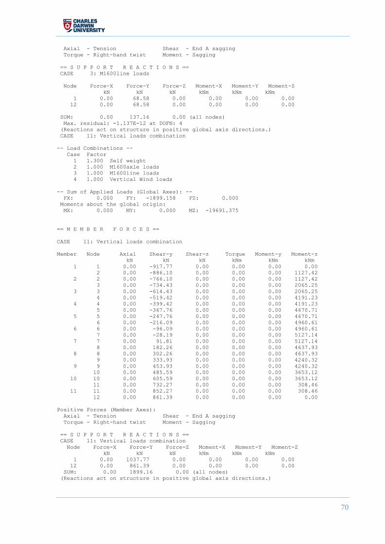
70
Axial - Tension Shear - End A sagging
Torque - Right-hand twist Moment - Sagging
== S U P P O R T R E A C T I O N S ==
CASE 3: M1600line loads
Node Force-X Force-Y Force-Z Moment-X Moment-Y Moment-Z
kN kN kN kNm kNm kNm
1 0.00 68.58 0.00 0.00 0.00 0.00
12 0.00 68.58 0.00 0.00 0.00 0.00
SUM: 0.00 137.16 0.00 (all nodes)
Max. residual: -1.137E-12 at DOFN: 4
(Reactions act on structure in positive global axis directions.)
CASE 11: Vertical loads combination
-- Load Combinations --
Case Factor
1 1.300 Self weight
2 1.000 M1600axle loads
3 1.000 M1600line loads
4 1.000 Vertical Wind loads
-- Sum of Applied Loads (Global Axes): --
FX: 0.000 FY: -1899.158 FZ: 0.000
Moments about the global origin:
MX: 0.000 MY: 0.000 MZ: -19691.375
== M E M B E R F O R C E S ==
CASE 11: Vertical loads combination
Member Node Axial Shear-y Shear-z Torque Moment-y Moment-z
kN kN kN kNm kNm kNm
1 1 0.00 -917.77 0.00 0.00 0.00 0.00
2 0.00 -886.10 0.00 0.00 0.00 1127.42
2 2 0.00 -766.10 0.00 0.00 0.00 1127.42
3 0.00 -734.43 0.00 0.00 0.00 2065.25
3 3 0.00 -614.43 0.00 0.00 0.00 2065.25
4 0.00 -519.42 0.00 0.00 0.00 4191.23
4 4 0.00 -399.42 0.00 0.00 0.00 4191.23
5 0.00 -367.76 0.00 0.00 0.00 4670.71
5 5 0.00 -247.76 0.00 0.00 0.00 4670.71
6 0.00 -216.09 0.00 0.00 0.00 4960.61
6 6 0.00 -96.09 0.00 0.00 0.00 4960.61
7 0.00 -28.19 0.00 0.00 0.00 5127.14
7 7 0.00 91.81 0.00 0.00 0.00 5127.14
8 0.00 182.26 0.00 0.00 0.00 4637.93
8 8 0.00 302.26 0.00 0.00 0.00 4637.93
9 0.00 333.93 0.00 0.00 0.00 4240.32
9 9 0.00 453.93 0.00 0.00 0.00 4240.32
10 0.00 485.59 0.00 0.00 0.00 3653.12
10 10 0.00 605.59 0.00 0.00 0.00 3653.12
11 0.00 732.27 0.00 0.00 0.00 308.46
11 11 0.00 852.27 0.00 0.00 0.00 308.46
12 0.00 861.39 0.00 0.00 0.00 0.00
Positive Forces (Member Axes):
Axial - Tension Shear - End A sagging
Torque - Right-hand twist Moment - Sagging
== S U P P O R T R E A C T I O N S ==
CASE 11: Vertical loads combination
Node Force-X Force-Y Force-Z Moment-X Moment-Y Moment-Z
kN kN kN kNm kNm kNm
1 0.00 1037.77 0.00 0.00 0.00 0.00
12 0.00 861.39 0.00 0.00 0.00 0.00
SUM: 0.00 1899.16 0.00 (all nodes)
(Reactions act on structure in positive global axis directions.)

71
(Basis for Section 4.2)
a
Longitudinal And Transverse Horizontal Loads on a Bridge Span (At the Superstructure)
Combination of Ultimate Loads on a Bridge Span
(Note: The Vertical loads have been modelled as uniformly distriuted load from the deck
onto the girders)
== I N P U T / A N A L Y S I S R E P O R T ==
Job: Load Combinations
Title: Ultimate Loads
Type: Space frame
Nodes ............................. 15
Members ........................... 22
Spring supports ................... 0
Sections .......................... 2
Materials ......................... 1
Primary load cases ................ 7
Combination load cases ............ 1
Analysis: Linear elastic
== L O A D C A S E S ==
Case Type Analysis Title
1 P L Transverse Wind Loads- ultimate
2 P L Longitudinal Wind Loads - ultimate
3 P L Self-weight

72
4 P L Braking Loads - Multiple
5 P L Drag Force Due to Water Flow - flood level
7 P L Vertical Wind Loads - ultimate
8 P L Traffic Loads
11 C L Title of case 11
Analysis Types:
S - Skipped (not analysed)
L - Linear
N - Non-linear
== N O D E C O O R D I N A T E S ==
Node X Y Z Restraint
m m m
1 0.000 0.000 0.000 111000
2 0.000 0.000 1.638 111000
3 0.000 0.000 3.277 111000
4 0.000 0.000 5.144 111000
5 0.000 0.000 7.010 111000
6 11.430 0.000 0.000 100000
7 11.430 0.000 1.638 100000
8 11.430 0.000 3.277 100000
9 11.430 0.000 5.144 100000
10 11.430 0.000 7.010 100000
11 22.860 0.000 0.000 111000
12 22.860 0.000 1.638 111000
13 22.860 0.000 3.277 111000
14 22.860 0.000 5.144 111000
15 22.860 0.000 7.010 111000
== M E M B E R D E F I N I T I O N ==
Member A B C Prop Matl Rel-A Rel-B Length
m
1 1 2 -Y 1 1 000000 000000 1.638
2 2 3 -Y 1 1 000000 000000 1.639
3 3 4 -Y 1 1 000000 000000 1.867
4 4 5 -Y 1 1 000000 000000 1.866
5 1 6 -Y 1 1 000000 000000 11.430
6 2 7 -Y 1 1 000000 000000 11.430
7 3 8 Y 2 1 000000 000000 11.430
8 4 9 Y 2 1 000000 000000 11.430
9 5 10 Y 2 1 000000 000000 11.430
10 6 11 Y 1 1 000000 000000 11.430
11 7 12 Y 1 1 000000 000000 11.430
12 8 13 Y 2 1 000000 000000 11.430
13 9 14 Y 2 1 000000 000000 11.430
14 10 15 Y 2 1 000000 000000 11.430
15 6 7 -Y 1 1 000000 000000 1.638
16 7 8 -Y 1 1 000000 000000 1.639
17 8 9 -Y 2 1 000000 000000 1.867
18 9 10 -Y 2 1 000000 000000 1.866
19 11 12 -Y 1 1 000000 000000 1.638
20 12 13 -Y 1 1 000000 000000 1.639
21 13 14 -Y 1 1 000000 000000 1.867
22 14 15 -Y 1 1 000000 000000 1.866
== S T A N D A R D S H A P E S ==
Section Shape Name Comment D1/D4 D2/D5 D3/D6
1 I/H 762X267UB147 comment 0.750 0.013 0.265
0.018 0.265 0.018
2 I/H 762X267UB197 comment 0.770 0.016 0.268
0.025 0.268 0.025
Dimension codes:
I/H - D1=D D2=Tw D3=Btf D4=Ttf D5=Bbf D6=Tbf
== S E C T I O N P R O P E R T I E S ==
Section Ax Ay Az J Iy Iz fact
m2 m2 m2 m4 m4 m4
1 1.882E-02 0.000E+00 0.000E+00 1.503E-06 5.596E-05 1.673E-03 1.000
2 2.492E-02 0.000E+00 0.000E+00 3.597E-06 8.045E-05 2.358E-03 1.000
== M A T E R I A L P R O P E R T I E S ==

73
Material E u Density Alpha
kN/m2 t/m3 /deg C
1 2.000E+08 0.2500 7.850E+00 1.170E-05
== T A B L E O F Q U A N T I T I E S ==
MATERIAL 1
Section Name Length Mass Comment
m tonne
1 762X267UB147 63.017 9.311 comment
2 762X267UB197 72.313 14.146 comment
---------- ----------
135.330 23.457
== C O N D I T I O N N U M B E R ==
Maximum condition number: 2.493E+03 at node: 10 DOFN: 3
== A P P L I E D L O A D I N G ==
CASE 1: Transverse Wind Loads- ultimate
-- Member Loads --
Member Form T A S F1 X1 F2 X2
1 UNIF FZ LO 14.443
2 UNIF FZ LO 14.443
3 UNIF FZ LO 14.443
4 UNIF FZ LO 14.443
-- Sum of Applied Loads (Global Axes): --
FX: 101.245 FY: 0.000 FZ: 0.000
Moments about the global origin:
MX: 0.000 MY: 354.865 MZ: 0.000
CASE 2: Longitudinal Wind Loads - ultimate
-- Member Loads --
Member Form T A S F1 X1 F2 X2
5 UNIF FZ LO -6.490
10 UNIF FZ LO 6.490
-- Sum of Applied Loads (Global Axes): --
FX: 0.000 FY: 0.000 FZ: 148.361
Moments about the global origin:
MX: 0.000 MY: -1695.771 MZ: 0.000
CASE 3: Self-weight
-- Member Loads --
Member Form T A S F1 X1 F2 X2
5 UNIF FY LO 6.000
6 UNIF FY LO 11.050
7 UNIF FY LO -11.050
8 UNIF FY LO -11.050
9 UNIF FY LO -6.000
10 UNIF FY LO -6.000
11 UNIF FY LO -11.050
12 UNIF FY LO -11.050
13 UNIF FY LO -11.050
14 UNIF FY LO -6.000
-- Sum of Applied Loads (Global Axes): --
FX: 0.000 FY: -1032.129 FZ: 0.000
Moments about the global origin:
MX: 3502.425 MY: 0.000 MZ: -11797.235
CASE 4: Braking Loads - Multiple
-- Member Loads --
Member Form T A S F1 X1 F2 X2
6 UNIF FX LO 22.830
8 UNIF FX LO -22.830
11 UNIF FX LO 22.830
13 UNIF FX LO -22.830
-- Sum of Applied Loads (Global Axes): --

74
FX: 0.000 FY: 0.000 FZ: 0.000
Moments about the global origin:
MX: 0.000 MY: -1829.760 MZ: 0.000
CASE 5: Drag Force Due to Water Flow - flood level
-- Member Loads --
Member Form T A S F1 X1 F2 X2
5 UNIF FZ LO -0.342
10 UNIF FZ LO 0.342
-- Sum of Applied Loads (Global Axes): --
FX: 0.000 FY: 0.000 FZ: 7.818
Moments about the global origin:
MX: 0.000 MY: -89.361 MZ: 0.000
CASE 7: Vertical Wind Loads - ultimate
-- Member Loads --
Member Form T A S F1 X1 F2 X2
5 UNIF FY LO 5.000
6 UNIF FY LO 5.000
7 UNIF FY LO -5.000
8 UNIF FY LO -5.000
9 UNIF FY LO -5.000
10 UNIF FY LO -5.000
11 UNIF FY LO -5.000
12 UNIF FY LO -5.000
13 UNIF FY LO -5.000
14 UNIF FY LO -5.000
-- Sum of Applied Loads (Global Axes): --
FX: 0.000 FY: -571.500 FZ: 0.000
Moments about the global origin:
MX: 1950.987 MY: 0.000 MZ: -6532.245
CASE 8: Traffic Loads
-- Member Loads --
Member Form T A S F1 X1 F2 X2
5 UNIF FY LO 17.280
6 UNIF FY LO 34.500
7 UNIF FY LO -34.500
8 UNIF FY LO -34.500
9 UNIF FY LO -17.280
10 UNIF FY LO -17.280
11 UNIF FY LO -34.500
12 UNIF FY LO -34.500
13 UNIF FY LO -34.500
14 UNIF FY LO -17.280
-- Sum of Applied Loads (Global Axes): --
FX: 0.000 FY: -3156.052 FZ: 0.000
Moments about the global origin:
MX: 10702.328 MY: -0.001 MZ: -36073.672
CASE 11: Title of case 11
-- Load Combinations --
Case Factor
1 1.000 Transverse Wind Loads- ultimate
2 1.000 Longitudinal Wind Loads - ultimate
3 1.200 Self-weight
4 1.000 Braking Loads - Multiple
5 1.000 Drag Force Due to Water Flow - flood level
7 1.000 Vertical Wind Loads - ultimate
8 1.000 Traffic Loads
-- Sum of Applied Loads (Global Axes): --
FX: 101.245 FY: -4966.106 FZ: 156.180
Moments about the global origin:
MX: 16856.227 MY: -3260.029 MZ: -56762.602
== M E M B E R F O R C E S ==
CASE 11: Title of case 11

75
Member Node Axial Shear-y Shear-z Torque Moment-y Moment-z
kN kN kN kNm kNm kNm
1 1 0.000000 0.189913 94.043961 0.167305 98.884651 0.214752
2 0.000000 0.189913 70.386322 0.167305 -35.783749 -0.096326
2 2 0.000000 0.244824 25.746429 0.450331 4.960060 0.126394
3 0.000000 0.244824 2.074357 0.450331 -17.839075 -0.274873
3 3 0.000000 0.276777 40.333904 0.367040 32.733105 0.296132
4 0.000000 0.276777 13.368821 0.367040 -17.398392 -0.220610
4 4 0.000000 0.530643 57.430733 0.479516 36.416924 0.378449
5 0.000000 0.530643 30.480097 0.479516 -45.603893 -0.611731
5 1 0.000000 431.113068 -43.967751 -0.214752 -98.884651 0.167305
6 0.000000 94.156662 34.122009 -0.214752 -42.616238 -3.002E+03
6 2 130.473450 508.155640 -7.056072 -0.222720 -40.743809 0.283025
7-130.473450 -94.891174 -7.056072 -0.222720 39.907101 -2.362E+03
7 3 0.000000-589.510620 9.091908 -0.571005 50.572178 0.083290
8 0.000000 13.536164 9.091908 -0.571005 -53.3483353291.777832
8 4-130.473450-548.399658 9.516005 -0.599059 53.815311 -0.112479
9 130.473450 54.647141 9.516005 -0.599059 -54.9526142821.683594
9 5 0.000000-405.874237 8.443434 -0.611731 45.603893 0.479513
10 0.000000 -68.917816 8.443434 -0.611731 -50.9045492713.916260
10 6 0.000000 94.156662 34.174919 0.214752 42.7878193001.749512
11 0.000000 431.113068 -43.914841 0.214752 98.451454 -0.167305
11 7 130.473450 -94.891174 -7.069632 0.222720 -39.9479102361.523438
12-130.473450 508.155640 -7.069632 0.222720 40.857986 -0.283027
12 8 0.000000 -13.536164 -9.079210 0.571005 -53.3023453291.777832
13 0.000000 589.510620 -9.079210 0.571005 50.473022 0.083290
13 9-130.473450 -54.647141 -9.497896 0.599059 -54.9024282821.683594
14 130.473450 548.399658 -9.497896 0.599059 53.658527 -0.112479
14 10 0.000000 68.917816 -8.542773 0.611731 -51.2218362713.916260
15 0.000000 405.874237 -8.542773 0.611731 46.422054 0.479513
15 6 -68.296928 188.313324 0.122448 0.000000 0.171576 -0.429504
7 -68.296928 188.313324 0.122448 0.000000 -0.028994-308.886719
16 7 -54.171227 -1.469025 -0.058635 0.000000 -0.069876-309.332153
8 -54.171227 -1.469025 -0.058635 0.000000 0.026227-306.924438
17 8 -36.000107 -28.541355 0.104262 0.000000 0.072213-308.066467
9 -36.000107 -28.541355 0.104262 0.000000 -0.122445-254.779739
18 9 -16.986214-137.835632 -0.208756 0.000000 -0.072258-255.977875
10 -16.986214-137.835632 -0.208756 0.000000 0.317281 1.223463
19 11 0.000000 0.189933 -84.376183 -0.167305 -98.451454 0.214774
12 0.000000 0.189933 -84.376183 -0.167305 39.756733 -0.096335
20 12 0.000000 0.244827 -13.563260 -0.450331 -1.101251 0.126394
13 0.000000 0.244827 -13.563260 -0.450331 21.128933 -0.274878
21 13 0.000000 0.276783 -27.799545 -0.367040 -29.344091 0.296138
14 0.000000 0.276783 -27.799545 -0.367040 22.557661 -0.220615
22 14 0.000000 0.530653 -41.544968 -0.479516 -31.100866 0.378456
15 0.000000 0.530653 -41.544968 -0.479516 46.422054 -0.611742
Positive Forces (Member Axes):
Axial - Tension Shear - End A sagging
Torque - Right-hand twist Moment - Sagging
== S U P P O R T R E A C T I O N S ==
CASE 11: Title of case 11
Node Force-X Force-Y Force-Z Moment-X Moment-Y Moment-Z
kN kN kN kNm kNm kNm
1 -94.043961 431.302979 -43.967751 0.000000 0.000000 0.000000
2 -85.833557 508.210541 -7.056064 0.000000 0.000000 0.000000
3 -38.259548 589.542603 -9.091928 0.000000 0.000000 0.000000
4 86.411537 548.653564 -9.516032 0.000000 0.000000 0.000000
5 30.480097 405.343597 -8.443461 0.000000 0.000000 0.000000
6 -0.122427 0.000000 0.000000 0.000000 0.000000 0.000000
7-260.765839 0.000000 0.000000 0.000000 0.000000 0.000000
8 -0.162901 0.000000 0.000000 0.000000 0.000000 0.000000
9 261.259918 0.000000 0.000000 0.000000 0.000000 0.000000
10 -0.208741 0.000000 0.000000 0.000000 0.000000 0.000000
11 84.376183 431.302979 -43.914841 0.000000 0.000000 0.000000
12-201.286362 508.210541 -7.069640 0.000000 0.000000 0.000000
13 14.236283 589.542603 -9.079229 0.000000 0.000000 0.000000
14 144.218872 548.653564 -9.497924 0.000000 0.000000 0.000000
15 -41.544968 405.343597 -8.542801 0.000000 0.000000 0.000000
SUM: -101.2454224966.106445-156.179657 (all nodes)
(Reactions act on structure in positive global axis directions.)

76
Appendix C. SPECIFIED PROPERTIES OF 8.8/TF BOLTS
The following tables include the specified values for the properties of Grade 8.8 bolts in accordance
with AS4192.
Chemical Composition
Material Treatment Carbon Steel with additives (e.g.
B, Mn or Cr) quenched and
tempered
Carbon Steel quenched
and tempered
Check
Composition
Limits %
(m/m)
C min 0,15 0,25
max 0,40 0,55
P max 0,035 0,035
S max 0,035 0,035
B max 0,003 0,003
Tempering Temperature
°C min
425 425
Mechanical and Physical Properties d≤16mm d>16mm
Nominal Tensile Strength (Rm,nom) N/mm2 800 800
Minimum Tensile Strength (Rm, min)= de N/mm2 800 830
Vickers Hardness, HV (F≥98N)
min 250 255
max 320 335
Surface Hardness HV 0,3 max not more than 30 Vickers points
above core hardness
Stress at 0.2% non-proportional elongation
Rp0,2 N/mm2
nom 640 640
min 640 660
Stress under proof load, Sp
Sp/R p0,2 0,91 0,91
N/mm2 580 600
Breaking Torque Mb Nm min See ISO898-7
Percent elongation after fracture, A min 12 12
Reduction area after fracture, Z %min 52
Strength under wedge loading
not smaller than minimum tensile
strength
Impact strength, Ku J min 30 30
Head soundness No fracture
Minimum height of non-decarburized thread zone, E ½ H1
Minimum depth of complete
decarburization, G
mm 0,015
Hardness after tempering
Reduction of hardness, 20 HV
maximum
Surface Integrity
In accordance with ISO 6157-1 or
ISO 6157-3 as appropriate

77
Appendix D. BOLTS, NUTS AND WASHERS INVENTORY
The diagram below shows the naming convention used in the bolt groups in the tabulated inventory.
Note: Old Beam (1,2,3) – those constructed in 1968
New Beam (4,5)– those constructed in 1972
Abutment 1 refers to the in-bound side (closer to Stuart Highway)
Section 1 refers to diaphragm section between Old beams 1 and 2, etc.
Bridge Section (All from Brace+Bottom Flange)
M16 M22 Observations
Notes on Diaphragm bolts Bolts Nuts Washers Bolts Nuts Washers
Abutment 1 New Beam 4A 8 8 10 0 2 0 None of the M16 washers have tabs
Abutment 1 New Beam 5A 4 4 6 0 4 0
Abutment 1 Old Beam 1A 4 4 8 0 3 2
Abutment 1 Old Beam 2A 8 8 16 0 4 4 Only 2 of M16 washers have tabs
Abutment 1 Old Beam 3A 8 8 14 0 4 4
Abutment 2 New Beam 4E 8 8 16 0 3 0
Abutment 2 NewBeam 5E 4 4 8 0 4 0 M22 nuts are badly corroded
Abutment 2 Old Beam 1E 4 4 8 0 4 4
Abutment 2 Old Beam 2E 8 8 17 0 3 5
Abutment 2 Old Beam 3E 8 7 16 0 4 3 M22 washers have no tabs and are corroded
Diaphragm 1 Section 1 12 12 24 4 4 7 complete
Diaphragm 1 Section 2 12 11 21 2 2 2 missing 2 M22
Diaphragm 1 Section 3 11 10 10 2 3 1 2 M16 bolts have failed in fatigue
missing 1 M16 and 2 M22
Diaphragm 1 Section 4 11 11 16 3 4 2 5 of the M16 washers were on their own (spares)
missing 1 M16 and 1 M22
Diaphragm 2 Section 1 12 12 24 4 4 8 1 set of M16 connection was not painted and had a smaller tab (recently replaced)
Complete
Diaphragm 2 Section 2 11 11 22 4 3 7 Missing 1 M16
Diaphragm 2 Section 3 12 12 24 4 3 8 Complete
Diaphragm 2 Section 4 12 12 24 4 4 5 Complete
Diaphragm 3 Section 1 12 11 21 4 4 8 1 M22 bolt was cut to be removed Complete
Diaphragm 3 Section 2 12 12 24 4 1 8 Complete
Diaphragm 3 Section 3 12 13 25 3 3 6 Missing 1 M22
Diaphragm 4 Section 1 20 20 10 4 4 8
M22 bolts are corroded and some necking. 1 M16 bolt failed (fatigue).
Diaphragm 4 Section 2 11 11 22 3 3 6 Bolts have corroded on some parts of the threaded section
missing 1 M16 and 1 M22
Diaphragm 4 Section 3 7 11 7 4 2 8
1 set of M16 connection without washers have fatigued (where neck and threaded area meets) Missing 5 M16
Diaphragm 4 Section 4 12 12 23 4 3 8 M22 bolts are more corroded than M16 bolts complete
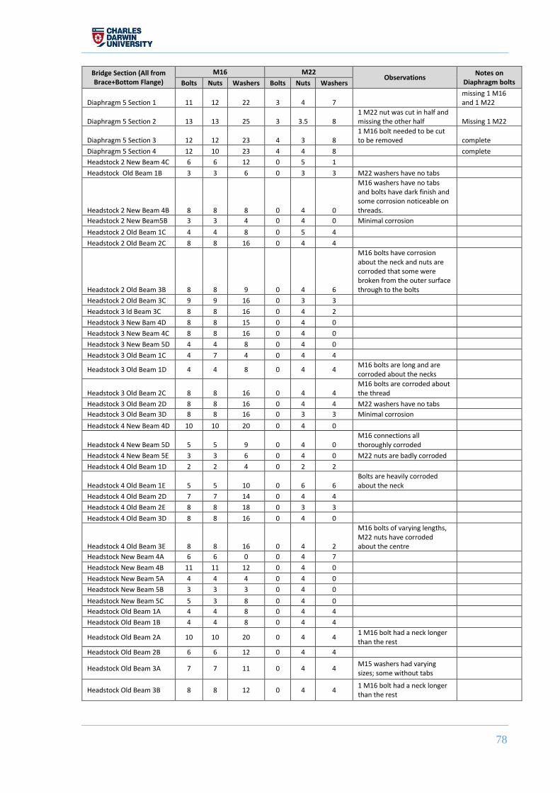
78
Bridge Section (All from Brace+Bottom Flange)
M16 M22 Observations
Notes on Diaphragm bolts Bolts Nuts Washers Bolts Nuts Washers
Diaphragm 5 Section 1 11 12 22 3 4 7 missing 1 M16 and 1 M22
Diaphragm 5 Section 2 13 13 25 3 3.5 8 1 M22 nut was cut in half and missing the other half Missing 1 M22
Diaphragm 5 Section 3 12 12 23 4 3 8 1 M16 bolt needed to be cut to be removed complete
Diaphragm 5 Section 4 12 10 23 4 4 8 complete
Headstock 2 New Beam 4C 6 6 12 0 5 1
Headstock Old Beam 1B 3 3 6 0 3 3 M22 washers have no tabs
Headstock 2 New Beam 4B 8 8 8 0 4 0
M16 washers have no tabs and bolts have dark finish and some corrosion noticeable on threads.
Headstock 2 New Beam5B 3 3 4 0 4 0 Minimal corrosion
Headstock 2 Old Beam 1C 4 4 8 0 5 4
Headstock 2 Old Beam 2C 8 8 16 0 4 4
Headstock 2 Old Beam 3B 8 8 9 0 4 6
M16 bolts have corrosion about the neck and nuts are corroded that some were broken from the outer surface through to the bolts
Headstock 2 Old Beam 3C 9 9 16 0 3 3
Headstock 3 ld Beam 3C 8 8 16 0 4 2
Headstock 3 New Bam 4D 8 8 15 0 4 0
Headstock 3 New Beam 4C 8 8 16 0 4 0
Headstock 3 New Beam 5D 4 4 8 0 4 0
Headstock 3 Old Beam 1C 4 7 4 0 4 4
Headstock 3 Old Beam 1D 4 4 8 0 4 4 M16 bolts are long and are corroded about the necks
Headstock 3 Old Beam 2C 8 8 16 0 4 4 M16 bolts are corroded about the thread
Headstock 3 Old Beam 2D 8 8 16 0 4 4 M22 washers have no tabs
Headstock 3 Old Beam 3D 8 8 16 0 3 3 Minimal corrosion
Headstock 4 New Beam 4D 10 10 20 0 4 0
Headstock 4 New Beam 5D 5 5 9 0 4 0 M16 connections all thoroughly corroded
Headstock 4 New Beam 5E 3 3 6 0 4 0 M22 nuts are badly corroded
Headstock 4 Old Beam 1D 2 2 4 0 2 2
Headstock 4 Old Beam 1E 5 5 10 0 6 6 Bolts are heavily corroded about the neck
Headstock 4 Old Beam 2D 7 7 14 0 4 4
Headstock 4 Old Beam 2E 8 8 18 0 3 3
Headstock 4 Old Beam 3D 8 8 16 0 4 0
Headstock 4 Old Beam 3E 8 8 16 0 4 2
M16 bolts of varying lengths, M22 nuts have corroded about the centre
Headstock New Beam 4A 6 6 0 0 4 7
Headstock New Beam 4B 11 11 12 0 4 0
Headstock New Beam 5A 4 4 4 0 4 0
Headstock New Beam 5B 3 3 3 0 4 0
Headstock New Beam 5C 5 3 8 0 4 0
Headstock Old Beam 1A 4 4 8 0 4 4
Headstock Old Beam 1B 4 4 8 0 4 4
Headstock Old Beam 2A 10 10 20 0 4 4 1 M16 bolt had a neck longer than the rest
Headstock Old Beam 2B 6 6 12 0 4 4
Headstock Old Beam 3A 7 7 11 0 4 4 M15 washers had varying sizes; some without tabs
Headstock Old Beam 3B 8 8 12 0 4 4 1 M16 bolt had a neck longer than the rest

79
Appendix E. EQUIPMENT USED FOR SAMPLE PREPARATION, BOLT ANALYSIS
AND BOLT TESTING
The above has been used for
metallographic preparation of test samples
as shown below.
Optical Microscope
Vickers Hardness Tester
sInstron machine and Actuator

80
Appendix F. VICKERS HARDNESS TESTING
Shown in this image is one of the results
from the Vickers Hardness Tests
conducted. The software is capable of
measuring the diagonals and
automatically calculating the hardness
number. The tensile strength (MPa) was
3.2x the Vickers Hardness.
Test Specimen Trial Diagonal Vickers Hardness Tensile Strength (Mpa) Average Tensile
Strength (Mpa)
1968 M22 Bolt
Thread 2 (Hv 1)
1 79.15 296 947.2
947.8
2 79.284 295 944.0
3 78.571 300 960.0
4 79.351 295 944.0
5 79.284 295 944.0
1972 M22 Bolt
Thread 1 (Hv
0,3)
1 45.974 263 841.6
891.5
2 43.636 292 934.4
3 45.455 269 860.8
4 44.156 285 912.0
5 44.286 284 908.8
1968 M22 Bolt
Cross-section 1
(Hv 0,3)
1 43.636 292 934.4
950.4
2 43.506 294 940.8
3 42.849 303 969.6
4 43.117 299 956.8
5 43.279 297 950.4
1972 M22 Bolt
Cross-section 2
(Hv 0,3)
1 79.15 296 947.2
947.8
2 79.284 295 944.0
3 78.571 300 960.0
4 79.351 295 944.0
5 79.284 295 944.0

81
Test
Specimen
Trial Diagonal Vickers Hardness Tensile Strength (Mpa) Average Tensile
Strength (Mpa)
1968 M16
Bolt 1
Cross-
section
1 44.104 286 915.2 935.7 2 43.352 296 947.2 3 43.799 290 928.0 4 43.279 297 950.4 5 43.574 293 937.6
1968 M16
Bolt 2
Cross-
section
1 44.654 279 892.8 923.5 2 43.723 291 931.2 3 43.45 288 921.6 4 43.723 291 931.2 5 43.5 294 940.8
1972 M16
Bolt 1
Cross-
Section
1 42.941 301 963.2 981.8 2 42.638 306 979.2 3 42.499 308 985.6 4 42.226 312 998.4 5 42.569 307 982.4
1972 M16
Bolt 2
Cross-
Section
1 42.708 305 976.0 988.8 2 41.958 316 1011.2 3 42.708 305 976.0 4 41.958 315 1008.0 5 42.778 304 972.8
1968 M16
Bolt Thread
1
1 40.935 332 1062.4 1029.3 2 42.778 304 972.8 3 41.121 329 1052.8
1968 M16
Bolt Thread
2
1 40.873 333 1065.6 1045.3 2 41.826 318 1017.6 3 41.121 329 1052.8
1972 M16
Bolt Thread
1
1 42.431 309 988.8 988.8 2 42.294 311 995.2 3 42.597 307 982.4
1972 M16
Bolt Thread
2
1 42.091 314 1004.8 996.3 2 42.849 303 969.6 3 41.892 317 1014.4

82
Appendix G. IMAGES FROM OPTICAL AND SCANNED ELECTRON MICROSCOPY
1968 5/8” Bolts Cross-Section
20x Magnification:
50x Magnification:
1968 5/8” Bolts Longitudinal Axis (Thread)
20x Magnification:
50x Magnification:
1972 M16 Bolts Cross Section
20x Magnification
50x Magnification

83
Appendix H. MECHANICAL TESTINGS
1. ONE SET OF SLIP LOAD GRAPH FROM THE SLIP TESTING EXPERIMENTS
2. FATIGUE TESTING EXPERIMENTAL DESIGN
M16 bolts (shear)
To determine the fatigue life of the M16 bolt group on the bridge diaphragm, a cyclic load experiment
is proposed to be conducted. Fatigue tests require the following parameters to be determined:
minimum load, maximum load and loading frequency.
Minimum and Maximum Load
The bolt group of 12 M16 bolts on the bridge diaphragms and the bolt group of 4 M16 on the gusset
plate connection at the inverse v-bracings are friction tightened and hence designed to resist slip at
load service and hence are designed to not be loaded over 70% of its slip load.
In conducting a fatigue test, the minimum and maximum loads in each cycle must be defined. In the
case of the M16 connections on the diaphragms, the minimum load is that of the dead loads and the
maximum is the 70% of the slip critical load. This 70% of the slip critical load is hence, for this
testing, assumed to be more than the dead load of the self-weight of the reinforced concrete deck and
the bridge railings together with the live loads of the traversing traffic causing the most adverse effect
on the structure. This is because the design factor only allow for bolted connections to not be loaded
more than 70% their capacity and as this connection is in shear, then that 70% is applied to its slip
critical load and not to its nominal shear capacity.
-10
0
10
20
30
40
50
60
70
80
90
-0.2 0 0.2 0.4 0.6 0.8 1 1.2 1.4
Load
(kN
)
Extension (mm)
First trials for M22 and 7/8" bolts
New
Old

84
The shear joints connecting the diaphragms and the main UB girders are subjected to the dead loads
due to the self-weight of the sections of the structure on top of the steel beams which include the
reinforced decking and the bridge railings which totalled up to 760kN per bridge span (total area of
168m2 and thus stress of 4.6MPa. The dead load due to 1/8 of the total area of the bridge span acts
on each set of bolted connection (21m2) thus total dead load each connection must resist is 4.6MPa x
21m2 = 96.6kN. There are 12 bolts in each of the diaphragm to girder bolted connection (6 on each
side) and hence each bolt is subjected to 8.05 kN each. However, it must be remembered that the total
strength of a bolt group of 12 bolts in one set of connection is not equal to 12 times the nominal
capacity of each bolt and that the stress concentration, shear and bending moment on each bolt in the
group varies depending on the bolt group centroid and the location of out-of-plain loading. For
simplicity, to carry out a cyclic loading test, it is important to use the maximum shear force on a bolt
in the group which in this case is that of the 8.05kN (as it would be acting on the bolts at the top or
closest to the location of the loading).
The maximum load is hence determined as the 70% of the slip critical load of the M16 friction
tightened bolts in double shear configuration. The slip resistance of an M16 bolt in a double shear
configuration was earlier calculated to be 29.47kN and as such its 70% is 20.6kN. From the slip tests
conducted on the new set of M16 bolts tightened such that the gap between the load indicating
washers and the plates was ensured to be at 0.25mm as specified for galvanized bolts, the average slip
load on 2 M16 bolts in a double shear configuration was 48kN implying that each bolt resisted 24kN
before slipping began, which is less than the 29kN as earlier calculated due to up to 20% inaccuracies
due to manual bolt tightening. As the average slip load from the earlier test is less than the determined
one from the calculated slip critical load, this will hence be the basis for the fatigue testing and as
such 70% of the 24kN will be used as the maximum load for the fatigue testing which is 16.8kN
From the above, the parameters for the fatigue testing of friction tightened bolt in an overlapped joint
is hence determined to have a minimum load of 8.05 kN and a maximum load of 16.8kN on each bolt.
However, as there are two bolts in the testing mechanism, for the fatigue testing, the loads will be at
minimum of 16.1kN and maximum of 33.6kN.
Loading Frequency and Expected Stress Cycle
From standards, service life of highways designed for Average Daily Truck Traffic (ADTT) of 2500
must be 2,000,000 cycles and those highways designed for ADTT of less than 2500 must have a
service life of 500,000 cycles.
Cyclic load testing requires for a pre-determined constant frequency for testing. For high-cycle
fatigue (HCF),20 to 50Hz is commonly used; however, this parameter is purely ideal and as such a
low-cycle fatigue (LCF) will instead be applied using a frequency of less than 10Hz,usually 0.01 to 5
Hz for a cycle of 10^4, however previous articles have conducted LCF testing in 5Hz and even up to
8-10Hz, which is usually indicated by the capacity of the testing machine or pre-determined based on
operation. As the lower frequency range in the LCF (0.01-5Hz) would imply stress cycles of less than
10^4, a loading frequency within the higher frequency range in the LCF (5-10Hz) would be chosen to
result in stress cycles in the 500,000 to 2,500,000 range.

85
Parameters:
Clamping force: Endure bolts are tightened such that the gap between the plate and the load indicating
washers is decreased down to 0.25mm
Minimum load: 16 kN
Maximum load: 33kN
Loading Frequency: 5-10 Hz (range can be smaller to ensure accuracy i.e. 5-6 or 8-10Hz depending
on machine)
Fatigue Testing for M22 bolts (tensile)
At the underside of each of the diaphragm-girder connections, there are 4 M22 bolts. For fatigue
testing, the amplitude for the cyclic loading would have a minimum of 0kN (as these connections are
not responsible for transfer of structural self-weight onto supports) and the maximum would be 1/4 of
the maximum horizontal braking forces (as there are 5 sets of this type of connection under each
diaphragm). The design horizontal braking force of the traffic condition with the highest vertical
loads on the structure was calculated to be 601.72kN which implies that each of the four bolt is
subjected to load of 150.4kN if only the braking force is considered. And as such for a cyclic tensile
testing of an M22 bolt the amplitude is 0kN and 150kN at 5-10Hz.
The maximum design axial tension of an M22 bolt with 0.8 factor (allowable maximum design load is
only 80% of nominal axial capacity) is 198kN. The 150.4kN due to horizontal braking forces is a lot
less than the design load which is still less than the axial capacity. However, if self-weight of the
structure and the other vertical loads on the bridge adds on to that load, the total applied load on the
M22 bolt at the diaphragm may very well be over the allowable maximum design load especially that
that location is where the maximum internal bending moment and maximum deflection of the bridge
occurs.