
BOEING VS AIRBUS: AN EMPIRICAL EXAMINATION A thesis submitted in
62
BOEING VS AIRBUS: AN EMPIRICAL EXAMINATION by Victor Dobrikov A thesis submitted in partial fulfillment of the requirements for the degree of Master of Arts in Economics National University “Kyiv-Mohyla Academy” Economics Education and Research Consortium Master’s Program in Economics 2005 Approved by ___________________________________________________ Ms.Svitlana Budagovska (Head of the State Examination Committee) __________________________________________________ __________________________________________________ __________________________________________________ Program Authorized to Offer Degree Master’s Program in Economics, NaUKMA Date __________________________________________________________
Transcript of BOEING VS AIRBUS: AN EMPIRICAL EXAMINATION A thesis submitted in

BOEING VS AIRBUS: AN EMPIRICAL EXAMINATION
by
Victor Dobrikov
A thesis submitted in partial fulfillment of the requirements for the degree of
Master of Arts in Economics
National University “Kyiv-Mohyla Academy” Economics Education and Research Consortium
Master’s Program in Economics
2005
Approved by ___________________________________________________ Ms.Svitlana Budagovska (Head of the State
Examination Committee)
__________________________________________________
__________________________________________________
__________________________________________________
Program Authorized to Offer Degree Master’s Program in Economics, NaUKMA
Date __________________________________________________________

National University “Kyiv-Mohyla Academy”
Abstract
BOEING VS AIRBUS: AN EMPIRICAL EXAMINATION
by Victor Dobrikov
Head of the State Examination Committee: Ms.Svitlana Budagovska, Economist, World Bank of Ukraine
This study considers the choice of an aircraft for different routes by airlines, in
light of recent realization of different strategies of main players in aircraft
production industry. Based on large sample of transatlantic flights from the US to
European countries by different airlines, results show positive relation between
probability of airlines choosing Airbus and average capacity of flights on that
route, European origin of an airline and departures frequency; negative relation
was found for the probability of choosing Airbus and distance of the route,
destination country GDP per capita and, most interestingly, flights from/to hub
airports and routes connecting two large airports. From the results of the study
we conclude that development of new products by aircraft producing companies
is based not on the future forecasts only but also on existing specifics of their
products exploitation.

TABLE OF CONTENTS
INTRODUCTION............................................................................................................ 1 LITERATURE REVIEW ............................................................................................... 7 DATA DESCRIPTION .................................................................................................16 METHODOLOGY ........................................................................................................24
4.1. Theoretical Background................................................................................24 4.2. Model Specification........................................................................................27
RESULTS...........................................................................................................................32 5.1. Estimation Results..........................................................................................32 5.2. Marginal Effects............................................................................................. 34
CONCLUSIONS..............................................................................................................39 BIBLIOGRAPHY ...........................................................................................................41 APPENDIX A .................................................................................................................43 APPENDIX B .................................................................................................................44 APPENDIX C .................................................................................................................45 APPENDIX D .................................................................................................................46 APPENDIX E .................................................................................................................47 APPENDIX F ..................................................................................................................48 APPENDIX G .................................................................................................................53 APPENDIX H .................................................................................................................54

LIST OF FIGURES AND TABLES
Number Page Figure 1. EADS and Boeing share prices 2 Figure 2. EADS and Boeing aircraft deliveries 5 Figure 3. Standard Normal and Logistic distributions 25 Figure 4. Marginal effects and Model coefficients 26 Table 1. Comparison of Airbus A380 and Boeing 747-400ER 3 Table 2. Probit model coefficients 32 Table 3. Marginal effects for BWL and HUB variables 34 Table 4. Marginal effects for OAL and EUAL variables 35 Table 5. Marginal effects for DIST and GDPPERCAPITA variables 37 Table 6. Marginal effects for ASEATS and DEPART variables 38
ii

ACKNOWLEDGMENTS
The author wishes to express his gratitude to his adviser, Dr. Volodymyr
Bilotkach, for his support, insightful comments and invaluable contribution to
this study by providing initial and main dataset. Special thanks are expressed to
Dr. Tom Coupe and Dr. Polina Vlasenko for their kind attention to the study and
useful comments during all the process of the thesis writing.
iii

GLOSSARY
Hub. An airport used by an airline to route its passengers within its network.
Hub-and-spoke network. Network within which passengers are routed through a single or multiple hubs.
VLA. Very large aircraft.
Wide-body aircraft. Aircraft with two or more aisles across the cabin.
Narrow-body aircraft. Aircraft with one aisle across the cabin.
Open skies agreement. Agreement between countries that liberalizes air connection between them allowing airlines from those countries to perform flights in/from and within partner country.
iv

C h a p t e r 1
INTRODUCTION
Many industries are close to duopolies with two firms serving almost the entire
market with other participants having negligible trading and production volumes.
The profound examples include UMC and Kyivstar on the Ukrainian mobile
communications market; Microsoft and Apple Computers in operating systems
industry, Intel and AMD in production of computer processors. The list can be
continued. Another example of such situation is the large civil aircraft industry,
most production in which is proposed by Boeing Commercial Aircrafts and
Airbus Industrie. While Boeing also has a military division producing missiles,
specialized jets, etc, the main focus of this paper will be on the civil part as both
firms are presented in the segment.
It is worth noting that competition between the companies is not only limited to
the usual market sphere, it is also strengthened by the fact that corporations are
situated in different regions of the world, Boeing in the USA (production in
Seattle, headquarters in Chicago) and Airbus in the EU (Toulouse, France), which
are both competing for the world economic leader position. This fact implies a
number of supporting programs for corporations, credits under special
conditions, subsidies, etc. This leads to frequent court visits on the issues of
“oversubsidizing” and free trade norms protection (first initiated by Airbus when
having minor positions on the market and recently renewed by Boeing when it
started losing its market positions). But, as usual, the final word for the success or
failure for the company’s product is to be said by the market. As can be seen
1

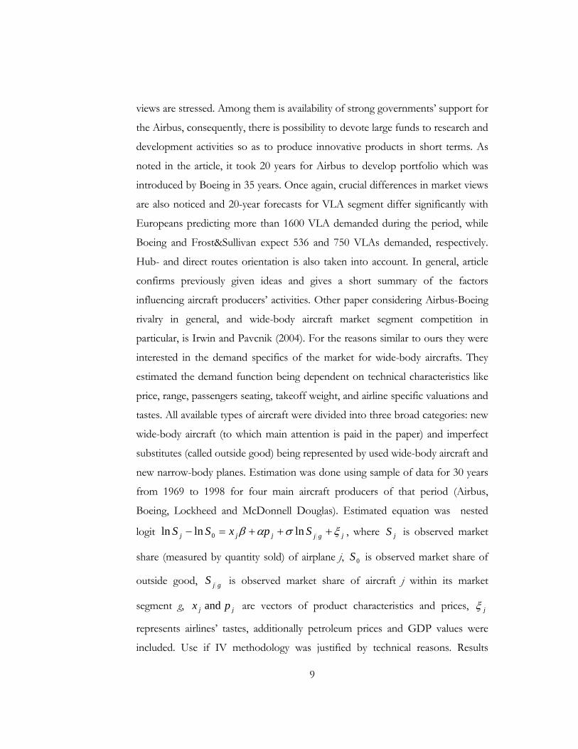
from the Figure 11, currently European company is more appreciated if deciding
on the basis of share price, which in many cases serve as a good estimator of the
company prospects estimator. And
here it comes to the main difference
between the competitors. They have
chosen different ways of developing
their products on the basis of their
vision of the development of the
passenger air transportation market in
the future. Airbus made a bet on the
hub-and-spoke system while Boeing
concentrated on fast direct flights,
which many customers prefer to indirect routes through hubs. Subsequently, they
developed quite different aircrafts. But the buyers for relatively large jets are not
so widely presented so as to have completely different customers for both
companies. There still is a choice for airlines to which strategy to stick to and
which airplanes to use to best fit their choice.
Figure 1 EADS and Boeing share prices
Recently both main market players presented their upper class jets. Boeing was
first with the upper midsize 7E7 Dreamliner (787 now, still not built) in
December 2004, followed by Airbus with giant super-jumbo A380 (already has a
plane, but not for the delivery) in January 2005. The aircrafts clearly demonstrate
the strategic choices of the producers; double-decker A380 can carry 555
passengers normally with maximum of incredible 840 for up to 15000 km, while
Boeing proposes about 300 seats and less distant flights readiness (slightly more
than 14000 km). The only plane by Americans being near A380 in size is old 747-
400ER with 416 passengers normal capacity (max 568) and slightly more than
14000 km distance of flight, but it was launched more than ten years ago and
1 Graph from The Economist, Jan 22nd 2004
2

currently no substitute for it is expected. Boeing’s aims are confirmed by
presentation on February 15, 2005 of the new member of the 777 family – 777-
200LR Worldliner with main advantage of extended range, now reaching almost
17500 km and giving possibility to connect virtually any two cities of the world by
direct flight with 301 passengers and revenue cargo on board. Main characteristics
of the companies’ largest planes are given below.
Table 1: Jumbos compared. Sources: Airliners.net, Wikipedia. Airbus A380-800 Boeing 747-400ER
Dimensions
Length 72.8 m 70.7 m Height 24.1 m 19.4 m
Wingspan 79.8 m 64.4 m Wing area 845 m2 541 m2
Cabin width 6.58 m 6.10 m Weights
Operating empty 277,000 kg 181,755 kg MTOW 540,000 kg 362,875 kg
Powerplants
No. engines 4 turbofans 4 turbofans Max engine thrust 374 kN (84,000 lb) 276 kN (62,000 lb)
Performance
Cruising speed 902 km/h 907 km/h Max speed 945 km/h 939 km/h
Range 14,800 km 14,205 km Capacity
Flightcrew 2 2 Seating (typical) 555 416 (23/78/315) Seating (max) 840 568
Cargo N/A 137-158.6 m3
It is obvious that aims of the companies differ much; Airbus targets long-haul
flights with hubs exploitation while Boeing is oriented on faster and more direct
flights. Both choices have their pros and cons. For the first one positive
distinction is possibility to have lower seat price due to lower in per seat terms
fuel expenditures which in light of oil becoming more and more expensive is
quite an important factor; second option has advantage in that most passengers
3

prefer to enter the board in their departure airport and leave it in the destination
place without having to waste time during additional stops in the hubs. From the
other point of view, advantage of one is disadvantage for another; A380
development can be additionally slowed by the fact that many of the airports are
currently technically not able to host it because of huge dimensions (mainly
weight). But most of them already caught the idea and are planning modifications
to meet the needs of the increased-size jets as they also suffer from the second
line airports improved positions caused by low-cost carriers’ expansion. As Eryl
Smith, Heathrow’s Director of business strategy, planning and development told
the Press Association: “A380 is critical for us”.
As was stated above, Boeing is not expected to present A380’s direct competitor
in the nearest future. Airbus, instead, already announced development of midsize
A350 which is expected to be a direct competitor for the 7E7 (however, there
was a rumor that such an announcement is nothing more than PR). Absence of
competing aircraft from Boeing may be explained by extremely large costs
associated with development of a jumbo. In this case, finally, Boeing’s small and
midsize aircraft will have to struggle with a bunch of direct competitors from
Airbus and A380 having no counterpart from Americans. Taking into account
the fact that in the industry usually some time is needed for an aircraft to be
actually launched after it’s official announcement (usually a few years, A380 will
be delivered to first customers in 2007 and 7E7 will be in line in 2010), current
actions and presentations can be seen as representing strategies for the nearest
decade(s).
Considering financial backgrounds of the companies, main dynamics of
improvement in Airbus’ positions along with weakening of the Boeing’s can be
noted. While still a leader in profits, Boeing already lost first position in
4

quantities2 (talking about large civil jets segment, in 2001 the number of orders
for Airbus jets exceeded number of orders for Boeing’s jets). In the recent years
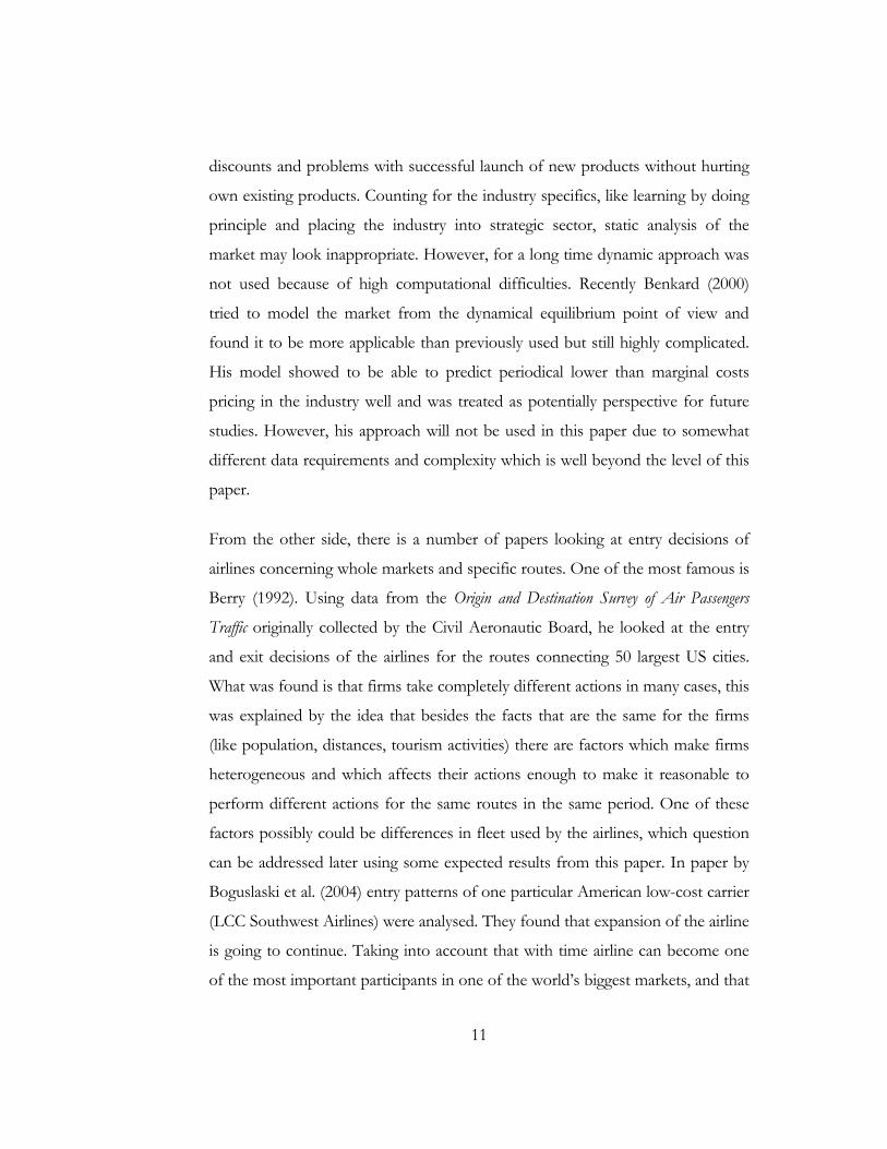
Airbus collected more orders for
their aircrafts but with high
discounts and high development
expenditures so that it did not allow
them to become a financial leader.
Now, main customers of the
European company by orders are
Lufthansa, Virgin Atlantic, Qantas,
Malaysian Airlines, Emirates and
Singapore Airlines. Other European
airlines (beside Lufthansa) are also
expected to order Airbus’ planes. Boeing recently allowed Japanese firms to take
close part in developing and producing 7E7 so as to create an additional incentive
for the Japanese airlines to purchase jets in which production Japanese companies
were involved. Talking about construction of the aircrafts we should note relative
magnitude of constructing expenses, and here Airbus with its $12bln spent on
A380 is ahead of American’s expenses for Dreamliner.
Figure 2 EADS and Boeing aircraft deliveries
So, this is the situation. The question is whether expected preferences of the
airlines are observed in reality. Our goal is to try to look at the same thing and
derive our conclusion on whether managers’ vision of the situation is in
accordance with real data. Question will be addressed in a quite standard manner
but using a rich dataset for the long period of time. In order to clarify the process
of estimation and unify the data, analysis will be limited to transatlantic scheduled
flights from the US. The rationale for such limitation of the sample is
straightforward: Europe and America represent a larger part of the world’s air
2 Graph from The Economist, Jan 20th 2005
5

travel market; most of the world’s largest airlines are situated in the US and the
EU; according to the data from Airports Council International, only 6 out of
world’s 30 busiest (as measured by the number of passengers arrived, departed
and transited) airports were not in the US or the EU (others in Asia). Exclusion
of charter flights is also logical as they do not represent regular or planned part of
the traffic and cannot be viewed as the determining part in the airlines decisions
on ways of flights development; also charter airlines have totally different
business models from that of the scheduled airlines. We expect to achieve reliable
results by using simple model with close attention paid to justification of
variables’ presence and functional form, which due to specifics of the data is
probit regression. So, we will check whether vision of each of aircraft producing
companies is in accordance with real data, for example is Airbus really used more
for flights into/out from the hubs or whether probability of flight performed
with Boeing increases with increase in distance of the flight.3 Our findings [shows
that there is positive relation between probability of Boeing aircraft exploitation
on a route and distance of that route and level of well-being in the destination
country (as measured by the GDP per capita), negative relation with average
flight capacity on a route, frequency of departures and European origin of an
airline. Unexpected result is that over the time period under consideration, hub
flights and routes connecting large airports had positive effect on probability of
Boeing exploitation.
3 Most of the facts in this chapter were taken from the various issues of The Economist magazine which
author will be happy to provide (in electronic form) by the first request
6

C h a p t e r 2
LITERATURE REVIEW
There is a number of papers considering airlines/aircraft industry. Interesting for
the current research and also close in idea is paper by Esty and Ghemawat (2002).
They concentrated on competition between the two main market participants in
very large aircraft segment, where now only Airbus is presented with the new
aircraft A380. Using game theory approach, decisions of the companies on
products launch/cancellation were analysed on the basis of empirical data. The
most striking finding was that it is possible to have potentially “more efficient”
player losing the product launch competition, as it actually happened with very
large aircrafts. As authors declared, two main questions to answer were why
Airbus, not Boeing did launch the super-jumbo and why did Boeing’s efforts to
launch intermediate product (known as “stretch jumbo”, being extended version
of 747) falter? Nice and wide overview of the history of development of the VLA
segment results in the conclusion that there were both similar opinions of the
companies’ management and differences. Common results of the considerations
were that there are prerequisites for the growth of the market for jumbos and that
the market for them will not be large enough to have room for more than one
producer. Differences, as we also noted were in that estimates for the demand for
VLA differed much across companies with Airbus predicting 3 to 4 times larger
figure. This was the main point from which strategies of the companies departed
in different destinations. Main factors included in the analysis were limited to
operating profits, sales ramp-up, launch costs, funding sources, discount rates,
terminal value, on-going expenditures and other variables consolidating
currencies, inflation, tax rates. These limitations were done in order to make
analysis more simple and tractable. As we can see authors’ approach differs from
7

our in that they concentrated on financial side and investment opportunities
valuation while our approach will look at the demand for the VLA side mainly
and airlines choices-influencing factors. Also their approach differs in
methodology as they have used game theory framework for making inferences
about producers’ decisions. Research produced the conclusion that despite the
fact that Boeing’s potential benefits from launching larger jumbo were higher
than Airbus’ it was not enough. Lack of strategic arguments and possibility of
temporary deterrence of the entry by using argument of cheap and efficient
modification of the existing aircraft by Boeing allowed them to deter new product
launch by competitors for some time and gain additional profits for some period
(actually about one year) without making any investment, just by speculating with
rumours and announcements. Also some insight on aircraft producers’ decisions
can be made by looking at the ideas presented by Benkard (2000). He considered
learning effects in the aircraft production industry using data from Lockheed and
found that there is evidence that aircraft production as a labour-intensive industry
is subject to changing production costs and possibilities depending on the
previous period’s overall production levels and production of some particular
types of aircraft in particular. He argues that in most cases there is a situation
where new jets development influences not only costs beared by the firm directly
but also affects other variable costs across the entire aircraft program. Hence, it is
the case that large variety of different modifications with the one model in an
unconstrained equilibrium is inefficient in that fewer modifications would allow
producers to have lower cost both through direct and indirect effects. This can be
tied to some Boeing’s problems as American product line includes more different
versions and modifications and also learning depreciation looks more likely to
happen within Boeing than within Airbus.
Some descriptive ideas on Boeing and Airbus competition are presented in an
article by Merluzeau (2004). Main differences in firms’ development and market
8
views are stressed. Among them is availability of strong governments’ support for
the Airbus, consequently, there is possibility to devote large funds to research and
development activities so as to produce innovative products in short terms. As
noted in the article, it took 20 years for Airbus to develop portfolio which was
introduced by Boeing in 35 years. Once again, crucial differences in market views
are also noticed and 20-year forecasts for VLA segment differ significantly with
Europeans predicting more than 1600 VLA demanded during the period, while
Boeing and Frost&Sullivan expect 536 and 750 VLAs demanded, respectively.
Hub- and direct routes orientation is also taken into account. In general, article
confirms previously given ideas and gives a short summary of the factors
influencing aircraft producers’ activities. Other paper considering Airbus-Boeing
rivalry in general, and wide-body aircraft market segment competition in
particular, is Irwin and Pavcnik (2004). For the reasons similar to ours they were
interested in the demand specifics of the market for wide-body aircrafts. They
estimated the demand function being dependent on technical characteristics like
price, range, passengers seating, takeoff weight, and airline specific valuations and
tastes. All available types of aircraft were divided into three broad categories: new
wide-body aircraft (to which main attention is paid in the paper) and imperfect
substitutes (called outside good) being represented by used wide-body aircraft and
new narrow-body planes. Estimation was done using sample of data for 30 years
from 1969 to 1998 for four main aircraft producers of that period (Airbus,
Boeing, Lockheed and McDonnell Douglas). Estimated equation was nested
logit jgjjjj SpxSS ξσαβ +++=− lnlnln 0 , where is observed market
share (measured by quantity sold) of airplane j, is observed market share of
outside good,
jS
0S
gjS is observed market share of aircraft j within its market
segment g, are vectors of product characteristics and prices, jj px and jξ
represents airlines’ tastes, additionally petroleum prices and GDP values were
included. Use if IV methodology was justified by technical reasons. Results
9

obtained showed possible positive dependency between market share and seats
number and range, negative relationships between market share and aircraft’s
price and petroleum price was in line with expectations. Coefficients for other
variables were insignificant. For the numerical results you are recommended to
check the original work. Also interesting point was that empirical justification to
the logical idea that higher degree of substitutability is present for the aircraft
within one class than for interclass was adopted. Positive evolution of own-price
elasticity showed that with time aircraft market becomes more sensitive to price
changes. Cross-price elasticities were much smaller and different for the products
of same segment and of different segments, latter being significantly larger.
Additionally, close look is made on same particularly important for Airbus-
Boeing competition events, such as 1992 US-EU aircraft pricing agreement and
launch of Airbus A380, a direct competitor for Boeing 747 model and the largest
super-jumbo in the industry. The 1992 subsidies-limiting agreement was found to
result in increased prices but the magnitude of this increase could not be
measured because of lack of necessary data. Simulation of A380 launch using
announced (at that time) characteristics showed up the facts that are currently
observed, namely, A380 undercutting smaller Airbus aircraft (A330 and A340)
because of large discounts proposed to gain large market share for the new
product right after presentation, along with lowering Boeing’s market share.
Overall effect was found to be positive for the European producer as their overall
market share was expected to increase. Estimates for super-jumbos market
capacity obtained in the paper are closer to those of Boeing but still accept the
hypothesis that Airbus will be able at least to cover their development costs ($12
billion). In the analysis idea that A380 launch was more strategic than financial
decision also appears, as producer’s presence in all market segments can serve as
additional reason for airlines to switch to their aircraft. Authors also support
original Benkard idea that too wide variety of the models in the producers’ line
cause some problems as well because of cross-model demand effects of price
10
discounts and problems with successful launch of new products without hurting
own existing products. Counting for the industry specifics, like learning by doing
principle and placing the industry into strategic sector, static analysis of the
market may look inappropriate. However, for a long time dynamic approach was
not used because of high computational difficulties. Recently Benkard (2000)
tried to model the market from the dynamical equilibrium point of view and
found it to be more applicable than previously used but still highly complicated.
His model showed to be able to predict periodical lower than marginal costs
pricing in the industry well and was treated as potentially perspective for future
studies. However, his approach will not be used in this paper due to somewhat
different data requirements and complexity which is well beyond the level of this
paper.
From the other side, there is a number of papers looking at entry decisions of
airlines concerning whole markets and specific routes. One of the most famous is
Berry (1992). Using data from the Origin and Destination Survey of Air Passengers
Traffic originally collected by the Civil Aeronautic Board, he looked at the entry
and exit decisions of the airlines for the routes connecting 50 largest US cities.
What was found is that firms take completely different actions in many cases, this
was explained by the idea that besides the facts that are the same for the firms
(like population, distances, tourism activities) there are factors which make firms
heterogeneous and which affects their actions enough to make it reasonable to
perform different actions for the same routes in the same period. One of these
factors possibly could be differences in fleet used by the airlines, which question
can be addressed later using some expected results from this paper. In paper by
Boguslaski et al. (2004) entry patterns of one particular American low-cost carrier
(LCC Southwest Airlines) were analysed. They found that expansion of the airline
is going to continue. Taking into account that with time airline can become one
of the most important participants in one of the world’s biggest markets, and that
11
this company almost does not explore hub routes, preferring direct flights, some
additional positive argument in favour of the Boeing strategy can be added to the
ones given before.
Yance (1972) postulated that airlines capacity is inflated by them until reaching
the break-even level determined by the costs and demand conditions. This fact
was explained by the idea that in such a way airlines try to secure themselves from
having lower capacities than are demanded by the market. In this way, we can
refer in our analysis to the idea that, by looking at the demand side of the market,
estimates of the future demand for the aircrafts of different sizes can be achieved
and, hence, potential gains for producers of different types of aircrafts can also be
estimated. Later paper by Baltagi et al. (1998) contains new non-standard
approach to the capacity issue. They used own-defined economic measures of
capacity utilization instead of standard engineering load factor. Two capacity-
utilization measures were calculated – demand-based measure and output-based
measure. The former was defined as revenue passenger miles divided by capacity
output and the latter as actual seat miles flown divided by capacity output.
Capacity output was estimated as the minimum average cost output. The most
interesting finding is that output-based capacity utilization coefficient of 1.0
(long-run equilibrium) corresponds to demand-based capacity utilization
coefficient of 0.65, implying that physical excess capacity has little in common
with economic one and, in essence, is quite a normal situation. This can be
explained by specific features of demand for air travel, where same flights but in
different time cannot be treated as perfect substitutes, common belief that
overcrowded flights are associated with lower quality of service (more obvious
for the case of restaurants, sporting events and cell phone communications). So,
according to the results, presence of empty seats in the flights is potentially
inevitable feature of the industry, thus increasing needed number of seats per
flight well beyond what would be needed if looking at the demand level only.
12

Daniel (1995) proposes congestion pricing for the main hub airports in order to
lower costs lost because of frequent delays caused by the fact that in many cases
one time period is attractive for many flights so that airports’ exploitation is
divided unequally in time. Using pricing mechanism dependent not only on
aircraft weight as it was before, but also congestion level at the arrival/departure
time, would allow smoothing out the demand for aircrafts’ presence in the
airports hence decreasing congestion and saving delays-caused losses. Possible
outcome of such decision would be moving of the origin/destination points to
the secondary airports in order to keep attractive schedule without increasing
costs; in which case additional limitations to the fleet type would possibly arise
due to lower technical level of secondary airports. So, airlines’ decision on fleet
type can be highly influenced by exogenous factors implied by indirect for airlines
reasons. Hendrics et al. (1995) approached the optimal structure of the airline
network using mathematical methods to find that, with no variable costs and
under assumption that passengers prefer less stops during the travel, hub-and-
spoke network is optimal from the point of view of monopolistic company
allowed to serve air connection between some number of cities. However, if
variable costs are not restricted to be zero, another optimal solution arises, being
the network with all cities connected directly. It is worth noticing that actually
competing aircraft producers in this case also have different points of view on
what optimum is observed by the airlines in that their recently presented products
are oriented on one of the two network configurations provided in the paper. It is
concluded that hubs network performs better with either high or low marginal
costs but not with intermediate level.
Airlines competition development for the American market was considered in
Borenstein (1992) and at that time it was found that despite the reasons that
caused deregulation in late 1970s, at the beginning of 1990s, industry became
heavily concentrated with possibility of needed regulation, ways out of the
13

situation were described to be in opening the market for another non-American
participants, improving access to the airports ground capacities and disclosure of
commission rates by the travel agents. Mostly this things has happened in the
time after paper was written, many open skies agreements were reached so that
large European carriers are able to perform flights in the US (see APPENDIX A
for the information on open skies agreements between the US and the European
countries). What is important for our topic is that increased possibilities for
foreign companies to act on the US air travel market to some extent justify our
sample as only flights from the US are taken into analysis. Marin (1995)
considered European airline market in view of prices and market structure and
also found that success of deregulation, in sense of higher efficiency, highly
depends on the equal availability of the airports facilities to market participants,
which in the time of article appeared were highly controlled by the national flag
carriers. Now, the situation is different, during recent years airports become more
easily available to all market participants and this also is a good sign for our
sample as such situation gives hope that it can be reasonable to make inferences
on its basis. Similar results were also obtained by Evans and Kessides (1993) for
their analysis of relation between dominance of an airline over an airport or over
particular city-pair route. They revealed that dominance of an airline over an
airport adds pricing power for that airline, while dominance over route does not
give such possibility. They concluded that perspective way for public policy
should be ensuring of equal access to the airports for different airlines in order to
improve air transportation industry performance. Ideas much like that described
are also present in Berry (1990) and Evans and Kessides (1994).
Golich (1992) looked at the problems arising from increased costs associated with
R&D activities, treatment of the aircraft production industries as strategically
important by governments and reached the conclusion that this sector should
expect internationalization, but without specifying how in particular the process
14

will be performed noting that development of an issue highly depends on the
decisions of policymakers of the countries with aircraft producing firms. Actually,
after the paper was written the situation developed by one of the scenarios
described. Firms’ evolution went so that currently two main players in the
industry are present, being object of attention in this work. Also, EU authorities
as well as US government see the industry as highly economically important with
all the implications of such a position, like subsidies, cheap credits, other kinds of
support and, of course, mutual court calls.
15

C h a p t e r 3
DATA DESCRIPTION
As previously noted, this paper relies on extensive dataset. In particular, originally
available data covered flights from the US airports to all the international
destinations, both scheduled and charter, for the period 1990-mid-2002, monthly.
These flights were described by number of passengers transported on a route,
number of seats available and number of departures. As data was monthly, it does
not represent each particular flight; rather activity of an airline on given route in
given month was described. After checking the data we found that period 1990-
1997 inclusively does not contain information on quantities of passengers
transported for the flights performed by non-American airlines. This caused
limitation of the sample to the time period 1998-mid-2002. Also we excluded
charter flights and flights performed by cargo airlines, postal services, etc. But still
main limitation was in using only data for transatlantic flights between US and
Europe. This decision was made after considering the fraction of American and
European long-haul flights market in overall long-haul flights market; another
important reason is that we consider flights between the aircraft producing
regions. These two markets present larger part of air transportation worldwide,
this can be illustrated by the fact that most of the world’s busiest airports are
situated in these regions (for information on world’s busiest airports as measured
by the passenger traffic, see APPENDIX B). After applying these limitations,
number of observations decreased to 11824 from initial 322019 (127522 for the
time period included in the sample), including observations on flights from 36
American origin airports to 49 destination airports in 23 European countries,
performed by 59 airlines, 12 of them American and 32 European with others
16

from Asia and Africa (for the list of airlines and their origin, see APPENDIX C).
This number of observations is still large enough to be representative for the
general situation and not experience any problems with number of variables.
Also, besides this dataset, we used data on orders and deliveries of Airbus and
Boeing planes, data on Open Skies Agreements, destination country per capita
GDP and international trade position, airport traffic. Finally, the set of variables
included fourteen variables (six of them being dummy variables) and whole set
(85) of dummies for destination airports. Namely, these are BOA, HUB, BWL,
PM, PAX, DEPART, DIST, LF, ASEATS, OSA, TRADE, GDPPERCAPITA,
NAMEUAL, EUAL and dummies for all airports, both origin and destination
(for the complete list of airports and cities, both American and European, see
APPENDIX D, later dummies for destination airports are called correspondingly
to their code; for origin airports first letter “d” is added).
BOA (stands for Boeing Or Airbus) is a dummy variable having value of either 0
or 1 (it is later used as a dependent variable). It shows whether flights in a given
month on a given route by a given airline were performed with Boeing
(corresponds to value 0) or Airbus (corresponds to value 1) aircraft. Of all 11824
observations, 6474 (54.75%) are with zeroes, 5350 (45.25%) with unity. This
shows that at the time period under consideration more airlines exploited Boeing
aircraft for more routes. However, these values correspond to 364111 and
408893 departures respectively, indicating that on average each airline company
on each route performed more flights per month with Airbus planes
(approximately 76), than those using Boeings (approximately 56).4 This variable
was derived from the data on orders, deliveries and in-operation for Airbus and
Boeing aircraft. For the airlines using both types of aircraft, distinction was made
on the basis of the average number of seats per flight, as models of aircraft have
4 You can find frequencies and cross-tabs for dummy variables in APPENDIX F
17

different typical capacity. Some information on Airbus and Boeing aircrafts
capacity and range can be found in APPENDIX E.
HUB is also a dummy which indicates whether origin or destination airport is
considered as a hub (value 1) or not (value 0). This variable was created basing on
the information which airports are used by particular airlines as hubs as suggested
by the structure of the airline’s network. For the American airlines it was
composed so that hubs for AA are ORD, DFW, MIA ant STL; for CO hubs are
EWR and IAH; for DL – ATL and CVG; for NW – DTW, MEM and MSP; for
UA – ORD, DEN and SFO and for US – PHL, PIT and RDU. For the
European airlines construction of the variable is straightforward (like BA and VS
– LHR, LH – FRA, AF – CDG, etc.). 5477 (46.32%) of observations represent
flights from/to the hubs.
BWL (stands for BetWeen Large) is one more dummy indicating if the route
connects two large airports, which belong to the group of top 10 world’s busiest
airports (we compared data on world’s largest airports for 2000-2002 and found
that top 10 list remains almost constant, exception is SFO, which was in the list in
2000 but later changed by DEN). From our sample, 1515 (12.81%) of
observations have value of unity for this variable, indicating route connecting two
large airports; this corresponds to 15 routes, which represent nearly 16% of all
the departures and passengers transported.
Two latter variables may seem highly related, but in fact they represent different
effects. HUB corresponds to airline network specific factors, while BWL reflects
that airports connected by the route are large. This factor may become especially
important for A380 (because of huge weight of the aircraft) which will be
launched in 2007; potentially there may be relation between the size of the
airports and aircraft used for flights on a route during the time period under
consideration.
18

PM (stands for Passenger Miles) is a variable formed by multiplying quantity of
passengers transported on a given route by distance of that route. It is expected
to reflect the scale of activity of an airline on a route. This number varies much
and depends on how many flights an airline performs on a route and how large
the distance between the origin and destination airports is5.
PAX describes how many passengers were transported on a given route by an
airline in each month when flights on that route happened. Like PM, it
characterizes the level of airline activity on a route in a given month. It also varies
much and depends largely on number of flights performed on a route. Also it is
closely related to the load factor, together with number of seats determining
average load factor for route by airline in each month.
DEPART is a variable which shows how frequently flights on a given route are
scheduled by a given airline over a month. It varies from 4 to 493, showing that
most frequent departures on a route were on average scheduled 16 times a day.
Such frequent flights correspond to British Airways on a route New York (JFK)
– London (LHR). Average number of the variable is 65, indicating that
connection between two regions is quite intensive, as on average two departures
per day are scheduled from the US airports for each route in each time period for
each airline presented on a route.
DIST is variable describing distance between origin and destination cities. It was
collected by myself using database on distance between large cities of the world.
It does not pretend to be precise distance between airports as they are frequently
situated in the suburbs, but few kilometers difference is relatively too small to
play an important role in further results. Range of routes differs much being from
4676 km to 10200 km with the mean of 6893 km. Shorter routes are mostly
5 You can find descriptive statistics for non-dummy variables in APPENDIX G
19

presented by flights connecting USA eastern coast with UK, longer are from
other regions to Germany and Eastern European countries.
LF (stands for Load Factor) is the variable created by dividing quantity of
passengers actually transported by number of seats available. Obviously, its value
falls between zero and unity. In this paper the load factor used is not the load
factor for each departure. Due to specifics of the data, load factor shows average
utilization of seats capacity for each route by each airline over a month. Value
varies from miserable 5.6% to 100%. Mean of 75.6% is quite high and reflects
possibility for further development of jet capacity or flights frequency. Relatively
low standard deviation shows that large part of observations is near high mean.
ASEATS (stands for Average SEATS) was formed by dividing number of seats
available on a route over month by number of departures on a route. This simply
shows how large an aircraft is used by the airline. It should be noted that as we
are interested in market for large aircraft, we excluded observations with value of
this variable of less than 200. It represented quite a small part of all observations.
Average number of seats for all flights connected with our sample is above 280,
with maximum of 529. Standard deviation is not very large. This shows that for
most flights popular models of aircraft were used. However, there are exceptions
like Virgin Atlantic using only very large aircrafts with more than 350 seats. For
this variable possible question may be why there are values with decimals. But
this is explained by average character of the variable, counting that different
aircrafts of the same model/producer can have slightly different number of seats,
also we should count for possible insignificant mistakes in the number of seats
offered over month values.
OSA (stands for Open Skies Agreement) is a dummy variable which indicates
whether in particular month Open Skies Agreement between the USA and the
destination country was present (value 1) or not (value 0). It takes value of unity
20

for 5969 (50.48%) observations. Obviously, number of agreements increases over
time and, consequently, fraction of unity values is higher than average in later
months and lower than average for the starting periods.
TRADE is a variable which represent total international trade turnover of the
destination country, measured as sum of exports and imports, quarterly. So, it
shows trade turnover of the country over the quarter in which month of
observation is. This data is collected from the International Financial Statistics
directory published by the International Monetary Fund monthly and covering
detailed data for several years before the publication. It was processed so as to
transform it to some comparable units, by converting values into dollars using
relevant exchange rates also available in the directory. Variable is usually
considered as a relevant indicator of scale of country’s participation in
international economical and business relations and, hence, can be expected to
show how much business travels are performed by the citizens of that country.
Obviously, values vary much as different countries are present in the sample as
destination points.
GDPPERCAPITA is a variable describing destination country’s internal well-
being, measured as GDP per capita in terms of constant 1995 US dollars,
quarterly. Mean is USD 5198 (note that this a high value as data is quarterly and
mean value corresponds to GDP per capita of USD 20808 if presenting annually)
indicating that most of the air connection happens with countries with highly
developed economies (we restricted the sample to US-Europe flights, but in
Europe we included countries such as Poland, Romania, etc., for which GDP per
capita is significantly lower than value mentioned above).
OAL (stands for Other AirLine) is a dummy variable, which indicates whether
observation corresponds to the non-American and non-European airline (value
21

1) or not (value 0). Of the entire sample, 898 (7.59%) has value of unity for this
variable.
EUAL (stands for EUropean AirLine) is also a dummy, indicating whether
flights on a route were executed by European airline (value 1) or not (value 0).
For 6830 (57.76%) observations this variable takes value of unity. Market share as
measured by quantity of passengers transported or seats proposed does not differ
much from frequencies for AMAL and EUAL variables showing similar load
factors and departures frequencies for American and European carriers.
Two latter variable frequencies do not sum up to the total number of
observations. Remaining observations corresponds to the flights performed by
the American airlines; they represent 4096 (34.64%) observations. We should
note that more activity in the market is undertaken by the European airlines. This
can be explained by the fact that there are more airlines from Europe presented
on the market. This, in turn, can be explained by the fact that they are mostly
smaller than large American carriers; also there is still legacy of European market
before the deregulation with each country having an airline (except Scandinavian
countries with SAS), requirement for an airline to be from the country where the
city is situated to be allowed to fly from that city to the US.
Other variables can be considered as a group as they are dummies for the
destination airports (1 for flight to that airport, 0 otherwise), there are 85 of them.
Four out of five most frequently visited airports in Europe are in top 10 busiest
airports of the world, one is in top 30. These airports are LHR (1647, 13.93%,
top 10), FRA (1503, 12.71%, top 10), AMS (1321, 11.17%, top 10), LGW (1247,
10.55%, top 30) and CDG (1121, 9.48%, top 10) and collectively represent 6839
(57.84%) observations. For the origin airports, two out of five most frequently
used for transatlantic flights airports are in top 10 world’s busiest airports and
two in top 30. These are JFK (2149, 18.17%, top 30), EWR (1348, 11.40%, top
22

30), ORD (1263, 10.68%, top 10), LAX (793, 6.71%, top 10), IAD (762, 6.44%)
and together represent 6315 (53.41%) observations. Comparing these we can
note that it looks like airlines activities in Europe are more concentrated than in
the US for the flights on US-Europe routes.
We should also note from the cross-tabs in APPENDIX F that value of unity for
variable BOA (flights performed with Airbus jets) is more common together with
unity for HUB and BWL, than value of zero (flights with Boeings). This gives us
a sign of high possibility that hypothesis of positive correlation between Airbuses
exploitation and hub flights is actually observed. From the same appendix we can
find that presence of Open Skies Agreement is positively connected with activity
of European airlines on the market, as should be expected.
23

C h a p t e r 4
METHODOLOGY
Theoretical background
As you may note from the data description section, our dependent variable is a
dummy, or an indicator variable. This limits choice of tools that can be used for
an estimation procedure. Reasons of limitations and possible approaches to
estimation will be shortly described below; more attention will be paid to the
method used in this paper, namely probit. Most of the theoretical information in
this chapter was taken from Greene “Econometric Analysis”. Interested readers
should refer to that book, but any other literature considering estimation with
discrete dependent variable will work as well. Here we will limit our attention to
the models for binary choice as they are directly connected with this paper’s
method.
When it comes to the estimation of the models with discrete dependent variable
(binary choice in our case), exploitation of the simple techniques like OLS is not
suitable anymore. Reason for this lies in the very nature of such a model. Problem
is that with use of regression approach, estimating model
εββ +′== xxFy ),( , residual term ε is inevitably heteroscedastic in a way
that depends on the coefficients in the regression. As εβ +′x must be equal to
either 0 or 1, residual term ε equals either xβ ′− or xβ′−1 with probability
and respectively (where F is a function that shows the probability of
dependent variable taking value of unity). Further it is easy to show that in such a
case
F−1 F
[ ] )1( xxxVar ββε ′−′= . Next, and more troublesome, shortcoming is that
resulting coefficients combined with variables values cannot be restricted to the
24

[ ]1,0 interval, thus producing meaningless probabilities and negative variances.
Requirement for the model is to produce coefficients such that following
properties would be observed (in general case):
0)1Pr(lim,1)1Pr(lim ====−∞→′∞→′
YYxx ββ
for a given regressor vector. So, models
that rely on different distributions appeared. First one is based on the assumption
of normal distribution which is )()()1Pr( xdttYx
βφβ
′Φ=== ∫′
∞−, where last
notation is commonly used for the standard normal distribution, this model is
referred to as a probit model. Another version uses logistic distribution which is
presented as )(1
)1Pr( xe
eY x
x
ββ
β
′Λ=+
== ′
′
, with last notation being commonly
used for the logistic cumulative distribution function, this model is called logit
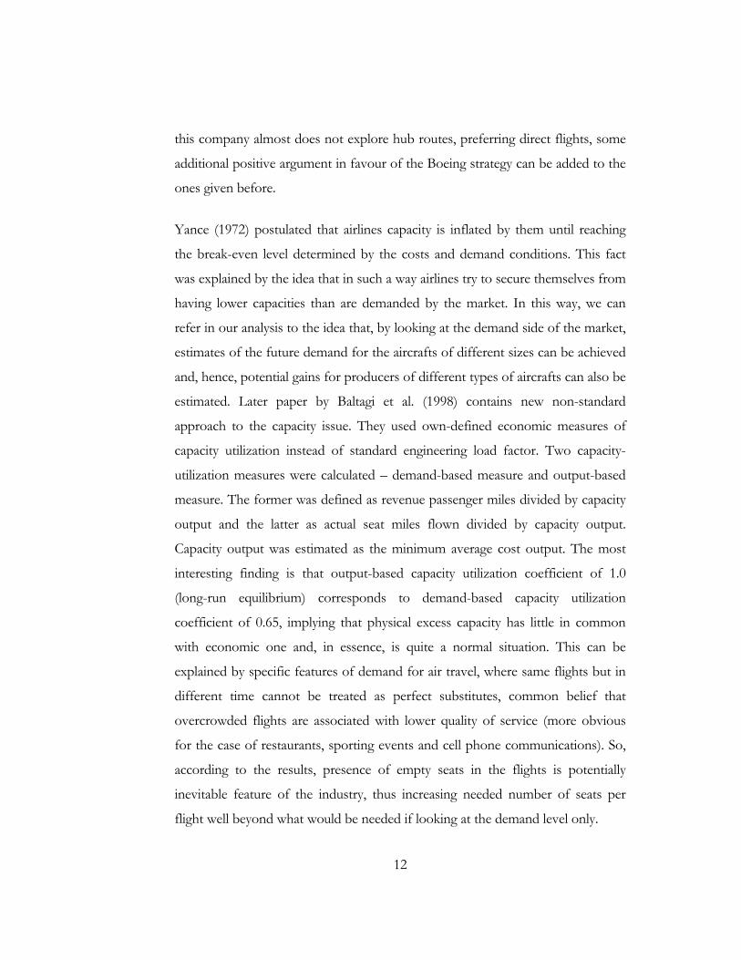
model. Two distributions are quite similar, but logistic has significantly heavier
tails, so that both distributions give similar probabilities to the intermediate
values, but
Standard Normal and Logistic Distributions with mean 0 and variance 1.435
0
0.2
0.4
0.6
0.8
1
1.2
-2 -1.8
-1.6
-1.4
-1.2 -1 -0
.8-0.6
-0.4
-0.2 0 0.
20.4
0.6
0.8 1 1.
21.4
1.6
1.8 2
Value of variable X
Pr(X
=x)
Standard NormalDistribution
Logistic Distribution
different for large or small values, this difference can be easily seen from the
Figure 3. Different outcomes from these models should be expected if: 1) there is
large inequality in the distribution of binary variable and 2) very large variation in
an important independent variable, especially if 1) is also present. Resulting
probability model is a regression [ ] [ ] [ ] )()(1)(10 xFxFxFxyE βββ ′=′+′−= ,
Figure 3
25

where is either standard normal or logistic distribution. Immediate result
from such specification is that parameters no longer represent usual marginal
effects directly. Now if we want to see how the dependent variable would change
in response to change in the regressor, we need to find the value of the following
derivative:
)(⋅F
[ ]βββ
ββ )(
)()( xf
xdxdF
xxyE
′=⎭⎬⎫
⎩⎨⎧
′′
=∂
∂ where is the density
function corresponding to the cumulative distribution,
)(⋅f
)(⋅F . For the normal
distribution assumed in probit models, this results in [ ]
ββφ )( xx
xyE′=
∂
∂, where
)(tφ is normal standard density; for the logistic distribution assumed in logit
models, we have [ ] [ )(1)()1( 2 xx
ee
xx
x
x
ββββ
β
β
′Λ−′Λ=+
=′∂′Λ∂
′
′
] and the result is
[ ] [ βββ )(1)( xx ]x
xyE′Λ−′Λ=
∂
∂. Obviously, values of these derivatives depend
on values of the variable and vary with them. They are mostly computed for the
mean values of the variable, other method is to calculate for each observation and
then get average of those marginal effects, for the large sample this methods
should give similar results. Computing marginal effects for some particular values
of the regressors is also convenient. Following figure illustrates graphically the
above description. On the graph it is easy to see the
Effect of variable X on Predicted Probabilities for variable Y
0
0.1
0.2
0.3
0.4
0.5
0.6
0.7
0.8
0.9
1 2 3 4 5
Variable Z
Pr(Y
=1)
With variable X
Without variable
Figure 4
26

difference between the coefficients from the model and corresponding marginal
effects. Horizontal difference between two curves is equal to the value of the
estimated coefficient for the variable X, while vertical distance between the
curves is marginal effect of the variable X on the probability of dependent
variable being equal to unity. Easy to see that marginal effect of the variable X
varies with changes in value of variable Z.
Estimation of the models is based on the method of maximum likelihood. Other
notes related to the probit and logit models are that it is not recommended to
exclude constant term from the estimation process unless this measure is justified
by the technical necessity (elimination of the collinearity, etc.). It is also desired to
have balanced dependent variable, e.g. with comparable number of observations
with value of zero and value of unity.
Model specification
As it was previously noted in this paper we will use relatively simple technique,
but it is quite appropriate for our data and purpose, so there is no need to
complicate things artificially. We will estimate probit model. For our large sample
with relatively balanced dependent variable (55% of observations have value of
zero and 45% has value of unity), even if we would use logit, it should give
similar results. So, the particular specification is:
∑=
+++++
++++++++++++=
61
1514131211
109876
543210
2^i
ii MYAIRPORTDUMOSALFDISTDIST
DEPARTPMPAXTAGDPPERCAPITRADEBWLHUBEUALOALASEATSBOA
βββββ
βββββββββββ
Note that we will include only 46 airport dummies in the model; this will be
explained later in the estimation results section. Model is specified so as to catch
27

possible influence from all the factors influencing decision on which aircraft to
use.
Remaining part of this chapter deals with the expected coefficients and reasons
for the expectations. These expectations are based on the information described
in the introduction, mainly beliefs about how and for which routes aircrafts of
two producers are used. So, main difference is that Airbuses are seen to be used
for flights in hub networks; consequently flights are shorter and quantity of
passengers transported per flight and in general on the route should be large.
Also, because of shorter flights, frequency should also be high and price lower
because of specifics of the hub networks. Boeings are seen as better for direct
flights connecting two end-points of the travel, hence less frequent, with smaller
capacity and more expensive. From these assumptions, the expected coefficients
are as follows.
Technical factors are presented by the DIST (distance between origin and
destination cities), DEPART (number of departures on a given route by a given
carrier monthly), ASEATS (average number of seats offered for flights on a
route for an airline monthly), LF (average load factor for flights by an airline on a
route monthly) and PAX (total quantity of passengers transported on a route by
an airline during a month) variables. They are expected to influence decision in a
way that limits choice to some particular models of aircraft that are better from
one or other aircraft producer (more suitable capacity, cruising speed, takeoff
weight, required frequency of service can be better for particular airline in one of
the producers aircraft). DIST should have negative effect on the probability of
exploitation of Airbus aircraft; this is a straightforward result from the
assumptions above. We expect to have coefficients with positive signs for
ASEATS, PAX and DEPART variables. For the LF we do not have strong
expectations but this factor is believed to have influence on aircraft choice.
28

TRADE (international trade turnover, measured as imports and exports in USD
in a destination country quarterly) and GDPPERCAPITA (per capita GDP in a
destination country quarterly) are expected to represent requirements of the main
customers for the air travel, showing up scale of business activity (and business
travels) and customers’ ability to pay respectively. These variables stand for the
part of business travel and ability to pay for the travel and should be positively
correlated with what is seen as Boeings’ specific – fast, direct and relatively
expensive flights (as should be true if decision on new products by aircraft
producers is made based on the available information for the previous products).
HUB (shows whether origin or destination airport is a hub for an airline that
performs flights on a route) and BWL (shows whether route connect two airports
from top 10 world’s largest airports or not) represent specifics of the flights and
airports that are connected by that flight. Expected sign for the HUB coefficient
is also directly driven by the assumptions, it should be positive. Coefficient for
the BWL variable should be positive as larger airports are associated with larger
scale of passenger transportation on a route and can possibly be used as hubs by
smaller airlines, not performing transatlantic flights but transporting passengers
from the large airports to the end-points of their travel.
Finally, PM (passengers transported over month on a route by an airline times
distance of the route), EUAL (shows whether observation is for the European
airline or not) and OAL (shows whether observation corresponds to activity of
non-American and non-European airline or not) represent regional specifics of
the airlines. First one is seen as representing airlines’ scale of activity and is
expected to have negative coefficient as large airlines are considered as more
conservative ones and move slowly to the new products (Airbus is new
comparing with Boeing). An expected coefficient of the latter variable is positive.
This is straightforward taking into account that Boeing is an American company,
29

while Airbus origin is Europe and that aircraft production is treated as a strategic
sector of the economy in both regions. There is a belief that American airlines
prefer Boeings other things being equal, while European ones favour Airbus. For
the OAL variable coefficient we do not have strong expectations, it is included in
order to allow us to see effect of an airline being from Europe influence the
probability of choice of an Airbus, comparing to the airlines from the US.
Constant term is preserved as it is not recommended to drop it for type of model
used here; a few control variables will be dropped to avoid collinearity (more on
this in the results section). For the OSA variable (indicates presence of Open
Skies Agreement between the US and the destination country) we would expect
positive coefficient if we would consider later period (Airbus gained much in sales
quantities on discounts, but this taken place after the time period considered
here). The reason is that the variable reflects the idea that the presence of Open
Skies Agreement tightens competition in the industry. Stronger competition leads
to higher attention to the problems of cost minimization and, hence, intensive
search for aircraft purchases under better terms. At that time period and previous
years (it takes some time to deliver an aircraft after an order), however, Boeing
was a leader in both quantities sold and revenues (from this we conclude that
Boeing offered better terms of purchases), so for this model we expect negative
coefficient of the variable. We believe that the factors named above collectively
determine which aircraft an airline would use for which route and, consequently,
purchases of that aircraft by the airline.
In the process of estimation, problem of possible inverse causality between
variables was considered; also we paid close attention to the clear and correct
determination of the variables. In the beginning HUB variable was specified
simply as large airport but after taking into account the fact that flights to some
large airport (CDG for example) are actually hub flights for some companies (AF
continuing with the example), but not so for other (BA, DL, LH, etc.). So, the
30

variable was reformulated to avoid this problem. Inverse causality is also not
expected to be present as actually decision on which aircraft to use is made with
other conditions (origin and destination, distance, expected capacity of the route,
type of travels on that route) being predetermined.
After obtaining coefficients from the model we will look at the marginal effects
of the variables. Of particular interest are marginal effects for the HUB, BWL,
OAL and EUAL variables. This will give possibility to say whether positive
relation between hub flights and Airbuses exploitation are observed in our sample
and whether preferences for aircraft produced in their regions are observed for
the airlines from the US and Europe or are just beliefs of the companies’
management. Also, it is interesting to see what is the direction and magnitude of
the effect of route connecting large airports.
31

C h a p t e r 5
RESULTS
Estimation Results
Before proceeding to the results of the estimation, let us shortly remind the idea
behind the model and main points that were checked. We look at the decisions of
the airlines on which aircraft to use for flights in relation with different factors
that should influence such decision. Our goal is too see what factors influence the
decision and in what manner. Main interest is in the marginal effects, which show
how presence of some factor influence the decision in favour of one of the
available aircraft types.
Below is the table with coefficient values for all the variables except control
variables and statistics on them (full estimation output can be found in
APPENDIX H). These results do not give final result but shows the direction in
which influence is observed.
Table 2. Coefficients from the probit model estimation
Variable Coefficient p-value Variable Coefficient p-value
ASEATS 0.000828 0.038 PM 0.0021131 0.146
HUB -0.6736826 0.000 PAX -0.0000339 0.008
OAL -0.309162 0.000 DEPART 0.0085643 0.000
EUAL 0.568899 0.000 DIST -0.0015451 0.000
BWL -0.9978611 0.000 DIST2 0.000000175 0.000
TRADE 0.00000467 0.051 LF 0.3686423 0.028
GDPPC -0.0004418 0.000 OSA 0.167449 0.082
32

From the table we can note that not all the coefficients are statistically significant,
also some of the estimated coefficients’ signs are not in accordance with
expectations. The model fits the data well as is indicated by relatively high value
of the R2 parameter which equals 0.4536. Important note is that before the
estimation we excluded a number of control variables as many of them have not
exhibited variation with the dependent variable (i.e. flights to Helsinki were
performed by Finnair Oy only and using Boeings only – hence no variation
between the regressand and the dummy for HEL is observed; similar case is with
some other destination and origin airports), a few were excluded in order to avoid
collinearity. As main interest for us lies in the marginal effects of the variables, we
will describe the coefficients just briefly. Most of them are significant at 5% level
of significance, hence affect the dependent variable. ASEATS,
GDPPERCAPITA, EUAL, DEPART and DIST have expected signs. Positive
values of the ASEATS, EUAL, and DEPART variables’ coefficients reflect
positive influence of this factors presence/increase on probability of choosing
Airbus. For the GDPPERCAPITA and DIST the effect is negative, thus
reflecting the negative effect of these factors on probability of choosing Airbus.
HUB, BWL and PAX variables have coefficients that differ from the expected.
These coefficients show negative for Airbus influence on aircraft choice. LF has
positive coefficient’s sign, for OAL the sign of the coefficient is negative.
TRADE, PM and OSA coefficients were found to be statistically insignificant. As
we previously noted main interest of this paper is represented by OAL, EUAL,
HUB and BWL variables.
Final step in estimation is to obtain the marginal effects of the regressors on the
dependent variable. As stated in the methodology section, the most common way
is to estimate marginal effect of the regressor with other independent variables
taken at their mean values. However, for our case this approach is not the best
one as we have dummies among the regressors and it is better to look at the
marginal effects for different values the dummies and their combinations.
33

Marginal Effects
We will start by examining the most interesting for us variables and their effect
on the choice of an aircraft. Below is a table with marginal effects for the HUB
(flights reformed through hub airport correspond to unity value) and BWL
(flights connecting two airports from the top 10 world’s largest airports
correspond to unity value) variables. We examined them for different values of
other main variables, all variables for which values are not mentioned are taken at
the mean values (except the cases when their values are obvious, like if
EUAL=1, then OAL=0 by construction of these dummies).
Table 3. Marginal Effects of HUB and BWL variables
BWL (p-values in parentheses) HUB (p-values in parentheses)
OAL=1, HUB=0 -0.0966374 (0.019) EUAL=1, BWL=0 -0.2101182 (0.000)
EUAL=1, HUB=0 -0.2742276 (0.000)
EUAL=1, HUB=1 -0.1313032 (0.006) EUAL=1, BWL=1 -0.0671938
(0.028)
OAL=0, EUAL=0, HUB=0 -0.1513567 (0.003) OAL=0, EUAL=0,
BWL=0 -0.1233843
(0.002)
OAL=0, EUAL=0, HUB=1 -0.050793 (0.045) OAL=0, EUAL=0,
BWL=1 -0.0228207
(0.098)
Most of the estimated marginal effects are significant at 5% level of significance;
insignificant is marginal effect of HUB for the case of American airlines’ flights
between large airports. Obviously, effects of the variables are negative. Of interest
here is magnitude of the effects and results for the different combinations of
other variables’ values. For the BWL variable the effect is negative but differs
much depending on other variables. Larger values correspond to flights
performed by the European airlines from/to non-hub airports, while lower
correspond to the airlines from other regions flights and flights from hubs.
Interesting feature is that BWL has the largest negative influence if combined
34

with non-hub flights performed by the European airlines. For the HUB variable,
effects pattern is similar. Larger negative values correspond to flights performed
by the European airlines. Actually these negative values give us possibility to
reject the idea that in the past choice of Airbus for the flights was favored by the
fact that the route is from/to hub airport or connects two large airports. Instead,
we observe an inverse relation – these factors increased probability of choosing
of Boeing aircraft for the flights. Despite the fact that these results sound
counterintuitive based on our assumptions, they are still easily explained. We
should note that in the time-period under consideration Boeing was undoubtedly
in the leading position and most of the large airlines used Boeing aircraft for their
flights, especially if looking at the aircraft with large capacity (e.g. more that 350
seats, until the presentation of A380 Airbus jets’ capacity didn’t exceed 380 seats
in standard configuration). Hence, the results reflect Boeing’s leading position in
the large airlines sector during the time period under consideration.
Next are the marginal effects for the OAL (flights performed by non-American
and non-European airlines) and EUAL (flights performed by an airline from
Europe) variables. They are constructed in the similar way - we examine cases of
different values for main variables while others are taken at their mean values).
Table 4. Marginal Effects of OAL and EUAL variables
OAL EUAL
OAL=0, HUB=1, BWL=0 0.0973134 (0.003) EUAL=0, HUB=0, BWL=0
-0.0693311 (0.004) OAL=0, HUB=1, BWL=1 0.0168032 (0.110)
OAL=0, HUB=0, BWL=0 0.1840473 (0.000) EUAL=0, HUB=0, BWL=1
-0.0146119 (0.096) OAL=0, HUB=0, BWL=1 0.0611764 (0.025)
We can see that the marginal effects of airlines origin indicators are positive for
European airlines and negative for non-American and non-European airlines;
some of them are statistically insignificant as indicated by high p-values. We
35

should note that these effects are comparing to the American airlines. So we can
conclude that airlines being from Europe favor Airbus more comparing to those
from the US, while airlines from other regions prefer Boeing, comparing to
American and European airlines. This is actually in line with our expectations
where we expected to observe European airlines preference for Airbuses if
compared with their American counterparts. Other important issue is that hub
routes decrease probability of Airbus exploitation; route connecting two large
airports also decrease probability of Airbus exploitation. General conclusion from
the table above is that we can accept the hypothesis stating that European airlines
exhibit preference to the European aircraft.
The following table presents marginal effects for DIST (distance between the
origin and destination cities) and GDPPERCAPITA (per capita GDP for the
destination country) variables. They are examined separately for airlines from
different regions; all other variables are taken at their mean values. Note that for
the DIST variable estimation of marginal effect is not straightforward, as we
included squared distance in our estimation to allow for non-linear effect of
distance. This variable has very small but positive coefficient. Hence, for marginal
effects of distance we estimate marginal effects of both DIST and DIST2 variables
and then look at the overall effect resulting from 1 km change in distance from
the mean value (6893 km). This way seem much wiser than estimating only
marginal effect for DIST without counting that it is to some extent outweighed
by the effect of DIST2. Also the effect of the change in distance differs depending
on from what distance the change happens, with larger (in absolute value) effects
corresponding to smaller distances and larger (in absolute value) effects
corresponding to larger distances. But as we noted in the data description chapter
and as can be seen from the APPENDIX G, standard deviation of the DIST
variable is not very large (1113), hence we suppose that estimating of marginal
effect at the mean value is reliable and values of the effect are applicable for most
36

of the observations. All the marginal effects for DIST and GDPPERCAPITA
variables are statistically significant at 5% level of significance.
Table 5. Marginal Effects of DIST and GDPPERCAPITA
DIST (modified) GDPPERCAPITA
OAL=1, EUAL=0 -0.000129448 (0.005) OAL=1, EUAL=0 -0.0000438
(0.026)
OAL=0, EUAL=1 -0.000380786 (0.000) OAL=0, EUAL=1 -0.0001290
(0.000)
OAL=0, EUAL=0 -0.00020651 (0.000) OAL=0, EUAL=0 -0.0000700
(0.005)
We can see that both variables affect the probability of Airbus choice in a way
that we have expected, for both variables the effect is negative. The effect is
larger (in absolute value) for the airlines from Europe and the lowest (in absolute
value) corresponds to airlines not from the US or Europe. Effects are negative
and show that increase in route distance by 100 km results in 1.29% to 3.81%
lower probability of choice of Airbus for that route. Increase of USD1000 in the
destination country’s per capita GDP per year results in 1.1% to 3.23% lower
probability of choice of Airbus for the route. These results are completely in
correspondence with our expectations and show that Boeings were preferred for
long routes with larger fraction of relatively rich passengers, that are able to pay
more for faster and direct flights.
Last pair of variables for which marginal effects are estimated is ASEATS
(average number of seats offered per flight on a route by an airline during a
month) and DEPART (number of departures on a route by an airline during a
month). They are estimated in a simple manner, without any complications,
separately for airlines from different regions, with all other variables taken at their
mean values.
37
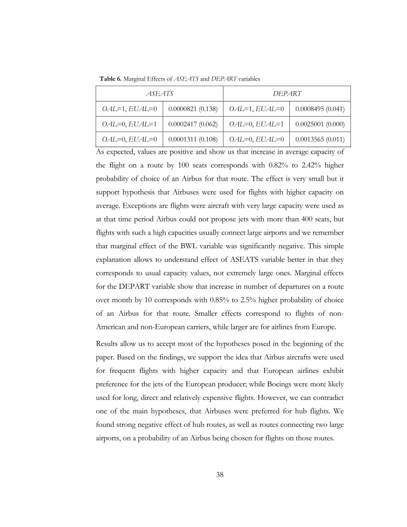
Table 6. Marginal Effects of ASEATS and DEPART variables
ASEATS DEPART
OAL=1, EUAL=0 0.0000821 (0.138) OAL=1, EUAL=0 0.0008495 (0.041)
OAL=0, EUAL=1 0.0002417 (0.062) OAL=0, EUAL=1 0.0025001 (0.000)
OAL=0, EUAL=0 0.0001311 (0.108) OAL=0, EUAL=0 0.0013565 (0.011)
As expected, values are positive and show us that increase in average capacity of
the flight on a route by 100 seats corresponds with 0.82% to 2.42% higher
probability of choice of an Airbus for that route. The effect is very small but it
support hypothesis that Airbuses were used for flights with higher capacity on
average. Exceptions are flights were aircraft with very large capacity were used as
at that time period Airbus could not propose jets with more than 400 seats, but
flights with such a high capacities usually connect large airports and we remember
that marginal effect of the BWL variable was significantly negative. This simple
explanation allows to understand effect of ASEATS variable better in that they
corresponds to usual capacity values, not extremely large ones. Marginal effects
for the DEPART variable show that increase in number of departures on a route
over month by 10 corresponds with 0.85% to 2.5% higher probability of choice
of an Airbus for that route. Smaller effects correspond to flights of non-
American and non-European carriers, while larger are for airlines from Europe.
Results allow us to accept most of the hypotheses posed in the beginning of the
paper. Based on the findings, we support the idea that Airbus aircrafts were used
for frequent flights with higher capacity and that European airlines exhibit
preference for the jets of the European producer; while Boeings were more likely
used for long, direct and relatively expensive flights. However, we can contradict
one of the main hypotheses, that Airbuses were preferred for hub flights. We
found strong negative effect of hub routes, as well as routes connecting two large
airports, on a probability of an Airbus being chosen for flights on those routes.
38

C h a p t e r 6
CONCLUSIONS
This study investigates the factors determining the decision of airlines on which
aircraft, Boeing or Airbus to use for different flights. We examined rich dataset
covering transatlantic flights by different carriers from the US to the European
countries for the recent time period, to find out main relations between the
airlines choices and different characteristics of the route for which the choice is
made and an airline itself. Among the main factors considered are distance,
passengers’ ability to pay, type of airports connected, average capacity of the
flights on a route and others.
We found that factors such as average capacity on a route, European origin of an
airline and departures frequency are positively related to the probability of
choosing Airbus for flights on that route; factors such as distance and destination
country GDP per capita are negatively related to probability of choosing Airbus
for flights on that route. The most interesting result is that negative relation
between hub flights and probability of choosing Airbus for those flights was
established; same relation was found for the flights connecting two large airports.
General conclusion is such that when deciding on future products, aircraft
producers account for existing relations and their actions are based on future
market forecast, as well as existing specifics of their products exploitation. So,
decision by Airbus to develop large aircraft is based, beside large estimated
capacity of the market for very large aircraft, on the facts that previously their
products were more likely used for relatively shorter flights with high capacity;
while Boeing executives decided on new extra-long-range aircraft development
taking into account that Boeing aircraft is preferred for relatively distant direct
39

flights with relatively low capacity. Unexpected negative relation between hub
flights and probability of choosing Airbus is explained by the idea that for hub
flights mostly aircraft with high capacity is used and over the previous period
Boeing produced larger jets that had no competitors from Airbus.
40

BIBLIOGRAPHY
Baltagi, Badi H.; Griffin, James M.; Vadali, Sharada R. Excess Capacity: A Permanent Characteristic of US Airlines?, Journal of Applied Econometrics, Vol.13, No.6, pp. 645-657, 1998.
Benkard, Lanier C. A Dynamical Analysis of the Market for Wide-Bodied Commercial Aircraft, NBER Working Paper 7710, 2000.
Benkard, Lanier C. Learning and Forgetting: The Dynamics of Aircraft Production, The American Economic Review, Vol. 90, No. 4, pp. 1034-1054, 2000.
Berry, Steven T. Airport Presence as Product Differentiation, The American Economic Review, Vol. 80, No. 2, Papers and Proceedings of the Hundred and Second Annual Meeting of the American Economic Association pp. 394-399, 1990.
Berry, Steven T. Estimation of a Model of Entry in the Airline Industry, Econometrica, Vol. 60, No. 4, pp. 889-917, 1992.
Boguslaski, Charles; Harumi Ito; Lee, Darin Entry Pattern in the Southwest Airlines Route System, Review of Industrial Organization, No. 25, pp. 317-350, 2004.
Borenstein, Severin The Evolution of U.S. Airline Competition, The Journal of Economic Perspectives, Vol. 6, No.2, pp. 45-73, 1992.
Daniel, Joseph I. Congestion Pricing and Capacity of Large Hub Airports: A Bottleneck Model with Stochastic Queues, Econometrica, Vol.63, No.2, pp. 327-370, 1995.
Esty, Benjamin; Ghewamat, Pankaj Airbus vs. Boeing in Super Jumbos: A Case of Failed Preemption, working paper 02-061, Harvard Business School, Strategy Working Paper Series, 2002.
Evans, William N.; Kessides, Ioannis N. Living by the “Golden Rule”: Multimarket Contracts in the U.S. Airline Industry, The Quarterly Journal of Economics, Vol. 109, No.2, pp. 341-366, 1994.
Evans, William N.; Kessides, Ioannis N. Localised Market Power in the U.S. Airline Industry, The Review of Economics and Statistics, Vol. 75, No.1, pp. 66-75, 1993.
Greene, William H. Econometric Analysis, 4 editionth , Prentice Hall, 2000.
Golich, Vicki L. From Competition to Collaboration: The Challenge of Commercial-Class Aircraft
41

Manufacturing, Industrial Organization, Vol.46, No.4, pp. 899-934, 1992.
Hendrics, Ken; Piccione, Michele; Guofu Tan The Economics of Hubs: The Case of Monopoly, The Review of Economic Studies, Vol. 62, No.1, pp. 83-99, 1995.
International Financial Statistics, vol. LIII, No. 12, December 2000, IMF Statistics Department
International Financial Statistics, vol. LV, No. 12, December 2002, IMF Statistics Department
Irwin, Douglas A.; Pavcnik, Nina Airbus versus Boeing Revisited: international competition in the aircraft market, Journal of International Economics, Vol.64, pp. 223-245, 2004.
Marin, Pedro L. Competition in European Aviation: Pricing Policy and Market Structure, The Journal of Industrial Economics, Vol. 43, No.2, pp. 141-159, 1995.
Merluzeau, Michel Boeing vs. Airbus: The Market will Tell, not the Press Offices, Frost&Sullivan, 2004
The Economist, various issues, 1998-2005
Yance, Joseph V. Nonprice Competition in Jet Aircraft Capacity, The Journal ofIndustrial Economics, Vol. 21, No. 1, pp. 55-71, 1972.
42

APPENDIX A
History of Open Skies Agreements between USA and European countries6
# Date Entity Remarks Total # of OSA
1 January 2002 France Open Skies Agreement 55 2 May 2001 Poland Open Skies Agreement 53 3 October 2000 Malta Open Skies Agreement 50 4 January 2000 Slovak Republic Open Skies Agreement 41 5 December 1999 Portugal Open Skies Agreement 40 6 November 1998 Italy Open Skies Agreement 32 7 December 1997 Romania Open Skies Agreement 27 8 February 1996 Germany Open Skies Agreement 12 9 December 1995 Czech Republic Open Skies Agreement 11 10 May 1995 Austria Open Skies Agreement 10 11 May 1995 Belgium Open Skies Agreement 9 12 May 1995 Denmark Open Skies Agreement 8 13 May 1995 Finland Open Skies Agreement 7 14 May 1995 Iceland Open Skies Agreement 6 15 May 1995 Luxembourg Open Skies Agreement 5 16 May 1995 Norway Open Skies Agreement 4 17 May 1995 Sweden Open Skies Agreement 3 18 May 1995 Switzerland Open Skies Agreement 2 19 February 1992 Netherlands Open Skies Agreement 1
6 Data from U.S. Department of Transportation
43

APPENDIX B
World’s busiest airports, 20027
Rank City (Airport) Total passengers 1 Atlanta (ATL) 76876128 2 Chicago (ORD) 66565952 3 London (LHR) 63338641 4 Tokyo (HND) 61079478 5 Los Angeles (LAX) 56223843 6 Dallas/Ft Worth Airport (DFW) 52828573 7 Frankfurt/Main (FRA) 48450257 8 Paris (CDG) 48350172 9 Amsterdam (AMS) 40736009 10 Denver (DEN) 35651098 11 Phoenix (PHX) 35547167 12 Las Vegas (LAS) 35009011 13 Madrid (MAD) 33913456 14 Houston (IAH) 33905253 15 Hong Kong (HKG) 33882463 16 Minneapolis/St Paul (MSP) 32628331 17 Detroit (DTW) 32477694 18 Bangkok (BKK) 32182980 19 San Francisco (SFO) 31456422 20 Miami (MIA) 30060241 21 New York (JFK) 29943084 22 London (LGW) 29628423 23 Newark (EWR) 29202654 24 Singapore (SIN) 28979344 25 Tokyo (NRT) 28883606 26 Beijing (PEK) 27159665 27 Seattle (SEA) 26690843 28 Orlando (MCO) 26653672 29 Toronto (YYZ) 25930363 30 St Louis (STL) 25626114
7 Data from Airports Council International
44

APPENDIX C
List of airlines
Code Airline Country Code Airline Country 6F Laker Airways USA LY El Al Israel Airlines Israel AA American Airlines USA LZ Bulgarian Airlines Bulgaria AF Air France France MA Malev Hungary AI Air India India MP Martinair Holland Netherlands AY Finnair Oy Finland NG Lauda Air Italy AZ Alitalia Italy NW Northwest Airlines USA BA British Airways UK NZ Air New Zealand New Zealand BD Bradley UK OA Olympic Airways Greece BG Biman Bangladesh Bangladesh OK Czech Airlines Czech Rep. CO Continental USA OS Austrian Airlines Austria CYQ Corse Air France PE Air Europe Italy DE Condor Flugdienst Germany PK Pakistan Airlines Pakistan DL Delta Air Lines USA PR Philippine Airlines Philippines EI Aer Lingus Ireland RJ Alia-Royal Jordanian Jordanian ET Ethiopian Airlines Ethiopia RO Tarom Romanian Romania FF Tower Air USA SK Scandinavian Airlines Denmark H2 City Bird USA SN Sabena World Air Belgium HY Uzbekistan Airways Uzbekistan SQ Singapore Airlines Singapore IB Iberia Air Lines Spain SR Swissair Transport Switzerland IJ Interjet USA SU Aeroflot Russia IW Aom Minerve France SV Saudi Arabian Airlines Saudi Arabia JK Spanair Spain TN Air Tahiti Nui Tahiti KL KLM Royal Netherlands TP TAP Airlines Portugal KM Air Malta Malta TW Trans World Airlines USA KU Kuwait Airways Kuwait TZ American Trans Air USA LG Luxair Luxembourg UA United Air Lines USA LH Lufthansa Germany US USAir USA LO LOT Poland UX Air Europa Spain LT Luftransport Germany VS Virgin Atlantic UK LX Translux Switzerland
45

APPENDIX D
List of airports and cities
Airport City, Country/State Airport City, Country AGP Malaga, Spain LUX Luxembourg, Luxembourg AMS Amsterdam, Netherlands MAD Madrid, Spain ANC Anchorage, Alaska, USA MAN Manchester, England, UK ARN Stockholm, Sweden MCO Orlando, Florida, USA ATH Athens, Greece MEM Memphis, Tennessee, USA ATL Atlanta, Georgia, USA MIA Miami, Florida, USA BCN Barcelona, Spain MLN Melilla, Spain BGR Bangor, Maine, USA MSP Minneapolis/St Paul, Minnesota, USA BHX Birmingham, UK MSY New Orleans, Louisiana, USA BOS Boston, Massachusetts, USA MUC Munich, Germany BRU Brussels, Belgium MXP Milan, Italy BSL Basel, Switzerland NCE Nice, France BUD Budapest, Hungary OAK Oakland, California, USA BWI Baltimore, Maryland, USA OPO Oporto, Portugal CDG Paris, France ORD Chicago, Illinois, USA CLT Charlotte, North Carolina, USA ORY Paris, France CPH Copenhagen, Denmark OSL Oslo, Norway CVG Cincinnati, Ohio, USA OTP Bucharest-Otopeni, Romania DEN Denver, Colorado, USA PHL Philadelphia, Pennsylvania, USA DFW Dallas/Ft Worth, Texas, USA PHX Phoenix, Arizona, USA DTW Detroit, Michigan, USA PIT Pittsburgh, Pennsylvania, USA DUB Dublin, Republic of Ireland PRG Prague, Czech Republic DUS Düsseldorf, Germany RDU Raleigh/Durham, North Carolina, USAEWR Newark, New Jersey, USA RSW Ft Myers, Florida, USA FAI Fairbanks, Alaska, USA SAN San Diego, California, USA FCO Rome, Italy SEA Seattle, Washington, USA FLL Ft Lauderdale, Florida, USA SFO San Francisco, California, USA FRA Frankfurt, Germany SLC Salt Lake City, Utah, USA GLA Glasgow, Scotland, UK SNN Shannon, Republic of Ireland GVA Geneva, Switzerland SOF Sofia, Bulgaria HAM Hamburg, Germany STL St Louis, Missouri, USA HEL Helsinki, Finland STN London, England, UK IAD Washington, D.C., USA STR Stuttgart, Germany IAH Houston, Texas, USA SUJ Satu Mare, Romania IEV Kiev, Ukraine TPA Tampa, Florida, USA JFK New York, New York, USA TRF Sandefjord, Norway KBP Kiev, Ukraine TSR Timisoara, Romania KRK Krakow, Poland TXL Berlin, Germany LAS Las Vegas, Nevada, USA VCE Venice, Italy LAX Los Angeles, California, USA VIE Vienna, Austria LGW London, England, UK WAW Warsaw, Poland LHR London, England, UK ZRH Zurich, Switzerland LIS Lisbon, Portugal
46

APPENDIX E
Airbus and Boeing aircraft capacity and range
Airbus Boeing
A300-600 747-400
Capacity, seats 266 Capacity, seats 416/524
Range, km 7700 Range, km 13450
A310 747-400ER
Capacity, seats 220 Capacity, seats 416/524
Range, km 9600 Range, km 14205
A330-200 757-300
Capacity, seats 253 Capacity, seats 243/280
Range, km 12500 Range, km 6287
A330-300 757-200
Capacity, seats 295/335 Capacity, seats 200/228
Range, km 10500 Range, km 7222
A330-300E 767-400ER
Capacity, seats 295 Capacity, seats 245/304/375
Range, km 13700 Range, km 10454
A340-600 777-300
Capacity, seats 380 Capacity, seats 368/451/550
Range, km 14640 Range, km 11029
47

APPENDIX F
Descriptive statistics for dummy variables (BOA, HUB, INTERHUB, OSA,
OAL, EUAL, AMAL and some airport dummies)
. tab boa BOA | Freq. Percent Cum. ------------+----------------------------------- 0 | 6,474 54.75 54.75 1 | 5,350 45.25 100.00 ------------+----------------------------------- Total | 11,824 100.00 . tab hub Hub | Freq. Percent Cum. ------------+----------------------------------- 0 | 6,347 53.68 53.68 1 | 5,477 46.32 100.00 ------------+----------------------------------- Total | 11,824 100.00 . tab bwl BWL | Freq. Percent Cum. ------------+----------------------------------- 0 | 10,309 87.19 87.19 1 | 1,515 12.81 100.00 ------------+----------------------------------- Total | 11,824 100.00 . tab osa OSA | Freq. Percent Cum. ------------+----------------------------------- 0 | 5,855 49.52 49.52 1 | 5,969 50.48 100.00 ------------+----------------------------------- Total | 11,824 100.00
48
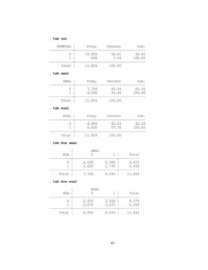
. tab oal NAMEUAL | Freq. Percent Cum. ------------+----------------------------------- 0 | 10,926 92.41 92.41 1 | 898 7.59 100.00 ------------+----------------------------------- Total | 11,824 100.00
. tab amal AMAL | Freq. Percent Cum. ------------+----------------------------------- 0 | 7,728 65.36 65.36 1 | 4,096 34.64 100.00 ------------+----------------------------------- Total | 11,824 100.00 . tab eual EUAL | Freq. Percent Cum. ------------+----------------------------------- 0 | 4,994 42.24 42.24 1 | 6,830 57.76 100.00 ------------+----------------------------------- Total | 11,824 100.00
. tab boa amal | AMAL BOA | 0 1 | Total -----------+----------------------+---------- 0 | 4,108 2,366 | 6,474 1 | 3,620 1,730 | 5,350 -----------+----------------------+---------- Total | 7,728 4,096 | 11,824 . tab boa eual | EUAL BOA | 0 1 | Total -----------+----------------------+---------- 0 | 2,916 3,558 | 6,474 1 | 2,078 3,272 | 5,350 -----------+----------------------+---------- Total | 4,994 6,830 | 11,824
49

. tab boa hub | Hub BOA | 0 1 | Total -----------+----------------------+---------- 0 | 3,886 2,588 | 6,474 1 | 2,461 2,889 | 5,350 -----------+----------------------+---------- Total | 6,347 5,477 | 11,824 . tab boa bwl | BWL BOA | 0 1 | Total -----------+----------------------+---------- 0 | 5,838 636 | 6,474 1 | 4,471 879 | 5,350 -----------+----------------------+---------- Total | 10,309 1,515 | 11,824 . tab osa amal | AMAL OSA | 0 1 | Total -----------+----------------------+---------- 0 | 3,631 2,224 | 5,855 1 | 4,097 1,872 | 5,969 -----------+----------------------+---------- Total | 7,728 4,096 | 11,824 . tab osa eual | EUAL OSA | 0 1 | Total -----------+----------------------+---------- 0 | 2,658 3,197 | 5,855 1 | 2,336 3,633 | 5,969 -----------+----------------------+---------- Total | 4,994 6,830 | 11,824
. tab lhr LHR | Freq. Percent Cum. ------------+----------------------------------- 0 | 10,177 86.07 86.07 1 | 1,647 13.93 100.00 ------------+----------------------------------- Total | 11,824 100.00
50

. tab fra FRA | Freq. Percent Cum. ------------+----------------------------------- 0 | 10,321 87.29 87.29 1 | 1,503 12.71 100.00 ------------+----------------------------------- Total | 11,824 100.00 . tab ams AMS | Freq. Percent Cum. ------------+----------------------------------- 0 | 10,503 88.83 88.83 1 | 1,321 11.17 100.00 ------------+----------------------------------- Total | 11,824 100.00 . tab lgw LGW | Freq. Percent Cum. ------------+----------------------------------- 0 | 10,577 89.45 89.45 1 | 1,247 10.55 100.00 ------------+----------------------------------- Total | 11,824 100.00 . tab cdg CDG | Freq. Percent Cum. ------------+----------------------------------- 0 | 10,703 90.52 90.52 1 | 1,121 9.48 100.00 ------------+----------------------------------- Total | 11,824 100.00 . tab djfk DJFK | Freq. Percent Cum. ------------+----------------------------------- 0 | 9,675 81.83 81.83 1 | 2,149 18.17 100.00 ------------+----------------------------------- Total | 11,824 100.00
51

. tab dewr DEWR | Freq. Percent Cum. ------------+----------------------------------- 0 | 10,476 88.60 88.60 1 | 1,348 11.40 100.00 ------------+----------------------------------- Total | 11,824 100.00
. tab dord DORD | Freq. Percent Cum. ------------+----------------------------------- 0 | 10,561 89.32 89.32 1 | 1,263 10.68 100.00 ------------+----------------------------------- Total | 11,824 100.00 . tab dlax DLAX | Freq. Percent Cum. ------------+----------------------------------- 0 | 11,031 93.29 93.29 1 | 793 6.71 100.00 ------------+----------------------------------- Total | 11,824 100.00 . tab diad DIAD | Freq. Percent Cum. ------------+----------------------------------- 0 | 11,062 93.56 93.56 1 | 762 6.44 100.00 ------------+----------------------------------- Total | 11,824 100.00
52

APPENDIX G
Descriptive statistics for non-dummy variables (PM, PAX, DEPART, DIST, LF,
ASEATS, TRADE, GDPPERCAPITA)
. sum pm pax depart dist lf aseats trade gdppercapita Variable | Obs Mean Std. Dev. Min Max -------------+-------------------------------------------------------- pm | 11824 9.65e+07 7.30e+07 510300 5.72e+08 pax | 11824 14157.66 10800.67 84 102504 depart | 11824 65.37585 46.14984 4 493 dist | 11824 6893.756 1113.916 4676 10200 lf | 11824 .7559337 .1294296 .0566572 1 -------------+-------------------------------------------------------- aseats | 11824 281.2301 67.26051 200 529.4 trade | 11824 1.34e+11 7.40e+10 2.02e+09 2.74e+11 gdppercapita | 11824 5198.309 1304.873 306 10924
53

APPENDIX H
Estimation results
Probit estimates Number of obs = 11824 LR chi2(60) = 7387.25 Prob > chi2 = 0.0000 Log likelihood = -4448.6444 Pseudo R2 = 0.4536 ------------------------------------------------------------------------------ boa | Coef. Std. Err. z P>|z| [95% Conf. Interval] -------------+---------------------------------------------------------------- aseats | .000828 .0003981 2.08 0.038 .0000478 .0016081 hub | -.6736826 .0512388 -13.15 0.000 -.7741088 -.5732565 eual | .568899 .0407781 13.95 0.000 .4889755 .6488226 oal | -.309162 .0734798 -4.21 0.000 -.4531797 -.1651443 bwl | -.9978611 .0880123 -11.34 0.000 -1.170362 -.8253602 trade | 4.67e-06 2.39e-06 1.95 0.051 -1.49e-08 9.35e-06 gdppercapita | -.0004418 .0000495 -8.92 0.000 -.0005388 -.0003448 pm | .0021131 .0014536 1.45 0.146 -.000736 .0049621 pax | -.0000339 .0000128 -2.65 0.008 -.000059 -8.81e-06 depart | .0085643 .0014422 5.94 0.000 .0057377 .0113909 dist | -.0015451 .0004326 -3.57 0.000 -.002393 -.0006972 dist2 | 1.75e-07 2.31e-08 7.58 0.000 1.30e-07 2.20e-07 lf | .3686423 .1674807 2.20 0.028 .0403861 .6968984 osa | .167449 .0963351 1.74 0.082 -.0213643 .3562622 ams | 11.0267 2.534416 4.35 0.000 6.059339 15.99407 arn | 8.886224 2.58162 3.44 0.001 3.826343 13.94611 ath | 8.232472 3.020837 2.73 0.006 2.311739 14.1532 bcn | 11.54235 2.605777 4.43 0.000 6.435122 16.64958 bhx | 11.91666 2.453574 4.86 0.000 7.107742 16.72557 bru | 7.647386 2.543849 3.01 0.003 2.661533 12.63324 cdg | 12.44738 2.550738 4.88 0.000 7.448025 17.44673 dub | 13.28785 2.341131 5.68 0.000 8.699319 17.87638 fco | 10.35723 2.789458 3.71 0.000 4.889992 15.82447 fra | 11.6405 2.685451 4.33 0.000 6.377115 16.90389 gla | 11.5696 2.3923 4.84 0.000 6.880782 16.25842 lgw | 11.28362 2.487287 4.54 0.000 6.408623 16.15861 lhr | 11.72426 2.486698 4.71 0.000 6.850425 16.5981 lis | 12.49746 2.445742 5.11 0.000 7.703896 17.29103 mad | 10.73255 2.482399 4.32 0.000 5.867138 15.59796 man | 12.02762 2.424528 4.96 0.000 7.275632 16.77961 muc | 8.58321 2.748077 3.12 0.002 3.197079 13.96934 mxp | 10.39372 2.683739 3.87 0.000 5.133692 15.65376 ory | 9.808126 2.560393 3.83 0.000 4.789848 14.8264 snn | 13.51679 2.291149 5.90 0.000 9.026219 18.00736 vie | 11.82864 2.755311 4.29 0.000 6.428331 17.22895 zrh | 9.580911 2.64742 3.62 0.000 4.392063 14.76976 datl | 3.70527 .3587046 10.33 0.000 3.002222 4.408318 dbos | 6.079515 .7037654 8.64 0.000 4.70016 7.45887 dbwi | 3.700078 .6132427 6.03 0.000 2.498144 4.902011 dclt | 3.529399 .4601889 7.67 0.000 2.627445 4.431353 dcvg | 3.302608 .4714397 7.01 0.000 2.378603 4.226613 dden | 3.60778 .2917913 12.36 0.000 3.03588 4.179681
54

ddfw | 6.626177 .3267133 20.28 0.000 5.985831 7.266524 ddtw | 4.772989 .5155882 9.26 0.000 3.762455 5.783523 dewr | 4.752872 .6216507 7.65 0.000 3.534458 5.971285 diad | 5.623337 .5440431 10.34 0.000 4.557032 6.689642 diah | 2.077614 .2663064 7.80 0.000 1.555663 2.599565 djfk | 4.783861 .6223743 7.69 0.000 3.56403 6.003692 dlas | 1.067988 .3425024 3.12 0.002 .3966953 1.73928 dlax | 2.245747 .401482 5.59 0.000 1.458857 3.032637 dmco | 3.479855 .3247934 10.71 0.000 2.843271 4.116438 dmem | 2.463279 .4891785 5.04 0.000 1.504507 3.422051 dmia | 4.168569 .302396 13.79 0.000 3.575884 4.761255 dmsp | 4.128614 .4488858 9.20 0.000 3.248814 5.008414 dord | 6.319589 .4422777 14.29 0.000 5.452741 7.186437 dphl | 5.284593 .5961719 8.86 0.000 4.116118 6.453069 dphx | .7946199 .3759992 2.11 0.035 .057675 1.531565 dpit | 4.32292 .5387339 8.02 0.000 3.267021 5.378819 dsea | 3.665931 .2782983 13.17 0.000 3.120476 4.211385 dsfo | 2.516873 .363122 6.93 0.000 1.805167 3.228579 _cons | -12.44144 . . . . . ------------------------------------------------------------------------------
55

4


![Airbus Boeing 23[1].](https://static.fdocuments.in/doc/165x107/54ce06cb4a79591e0f8b4992/airbus-boeing-231.jpg)