BIPEDAL ROBOT WALKING BY REINFORCEMENT LEARNING INPARTIALLY OBSERVED ENVIRONMENT

A THESIS SUBMITTED TOTHE GRADUATE SCHOOL OF APPLIED MATHEMATICS

OFMIDDLE EAST TECHNICAL UNIVERSITY

BY

UGURCAN ÖZALP

IN PARTIAL FULFILLMENT OF THE REQUIREMENTSFOR

THE DEGREE OF MASTER OF SCIENCEIN

SCIENTIFIC COMPUTING

AUGUST 2021

Approval of the thesis:

BIPEDAL ROBOT WALKING BY REINFORCEMENT LEARNING INPARTIALLY OBSERVED ENVIRONMENT

submitted by UGURCAN ÖZALP in partial fulfillment of the requirements for thedegree of Master of Science in Scientific Computing Department, Middle EastTechnical University by,

Prof. Dr. A. Sevtap Selçuk-KestelDirector, Graduate School of Applied Mathematics

Prof. Dr. Hamdullah YücelHead of Department, Scientific Computing

Prof. Dr. Ömür UgurSupervisor, Scientific Computing, METU

Examining Committee Members:

Assoc. Prof. Dr. Ümit AksoyMathematics, Atılım University

Prof. Dr. Ömür UgurScientific Computing, METU

Assist. Prof. Dr. Önder TürkScientific Computing, METU

Date:

iv

I hereby declare that all information in this document has been obtained andpresented in accordance with academic rules and ethical conduct. I also declarethat, as required by these rules and conduct, I have fully cited and referenced allmaterial and results that are not original to this work.

Name, Last Name: UGURCAN ÖZALP

Signature :

v

vi

ABSTRACT

BIPEDAL ROBOT WALKING BY REINFORCEMENT LEARNING INPARTIALLY OBSERVED ENVIRONMENT

ÖZALP, UGURCANM.S., Department of Scientific Computing

Supervisor : Prof. Dr. Ömür Ugur

August 2021, 56 pages

Deep Reinforcement Learning methods on mechanical control have been successfullyapplied in many environments and used instead of traditional optimal and adaptivecontrol methods for some complex problems. However, Deep Reinforcement Learn-ing algorithms do still have some challenges. One is to control on partially observ-able environments. When an agent is not informed well of the environment, it mustrecover information from the past observations. In this thesis, walking of BipedalWalker Hardcore (OpenAI GYM) environment, which is partially observable, is stud-ied by two continuous actor-critic reinforcement learning algorithms; Twin DelayedDeep Determinstic Policy Gradient and Soft Actor-Critic. Several neural architec-tures are implemented. The first one is Residual Feed Forward Neural Network underthe observable environment assumption, while the second and the third ones are LongShort Term Memory and Transformer using observation history as input to recoverthe hidden information due to the partially observable environment.

Keywords: deep reinforcement learning, partial observability, robot control, actor-critic methods, long short term memory, transformer

vii

viii

ÖZ

PEKISTIRMELI ÖGRENME YÖNTEMLERIYLE KISMI GÖZLENEBILIRORTAMDA ÇIFT BACAKLI ROBOTUN YÜRÜTÜLMESI

ÖZALP, UGURCANYüksek Lisans, Bilimsel Hesaplama Bölümü

Tez Yöneticisi : Prof. Dr. Ömür Ugur

Agustos 2021, 56 sayfa

Mekanik kontrol üzerine Derin Pekistirmeli Ögrenme yöntemleri birçok ortamda ba-sarıyla uygulanmıs ve bazı karmasık problemler için geleneksel optimal ve uyarla-nabilir kontrol yöntemleri yerine kullanılmıstır. Bununla birlikte, Derin PekistirmeliÖgrenme algoritmalarının hala bazı zorlukları vardır. Bunlardan bir tanesi, kısmengözlemlenebilir ortamlarda özneyi kontrol etmektir. Bir özne ortam hakkında yete-rince bilgilendirilmediginde, geçmis gözlemleri anlık gözlemlere ek olarak kullan-malıdır. Bu tezde kısmen gözlemlenebilir olan Bipedal Walker Hardcore (OpenAIGYM) ortamında yürüme kontrolü, iki sürekli aktör-elestirmen pekistirmeli ögrenmealgoritması tarafından incelenmistir; Ikiz Gecikmeli Derin Belirleyici Poliçe Grad-yanı (Twin Delayed Deep Determinstic Policy Gradient) ve Hafif Aktör Elestirmen(Soft Actor-Critic). Birkaç sinir mimarisi uygulanmıstır. Birincisi, gözlemlenebilir or-tam varsayımına göre Artık Baglantılı Ileri Beslemeli Sinir Agı iken ikincisi ve üçün-cüsü, ortamın kısmen gözlemlenebilir oldugu varsayıldıgından, gizli durumu kurtar-mak için girdi olarak gözlem geçmisini kullanan Uzun Kısa Süreli Bellek (LSTM) veTransformatördür (Transformer).

Anahtar Kelimeler: pekistirmeli derin ögrenme, kısmi gözlemlenebilirlik, robot kont-rolü, aktör-elestirmen metodları, uzun kısa süreli bellek, transformatör

ix

For anyone who is curious to read.

x

ACKNOWLEDGMENTS

I would like to thank my thesis supervisor Prof. Dr. Ömur Ugur whose insightfulcomments and suggestions were of inestimable value for my study. His willingnessto give his time and share his expertise has paved the way for me.

Special thanks also go to my friend Mehmet Gökçay Kabatas whose opinions andinformation have helped me very much throughout the production of this study.

I would also like to express my gratitude to my family for their moral support andwarm encouragements. Especially, I would like to show my greatest appreciation toSerpil Sökmen, who provides me to come these days.

Lastly, I would like to thank my partner Dilara Bayram for supporting me in longstudy days.

xi

xii

TABLE OF CONTENTS

ABSTRACT . . . . . . . . . . . . . . . . . . . . . . . . . . . . . . . . . . . . vii

ÖZ . . . . . . . . . . . . . . . . . . . . . . . . . . . . . . . . . . . . . . . . . ix

ACKNOWLEDGMENTS . . . . . . . . . . . . . . . . . . . . . . . . . . . . . xi

TABLE OF CONTENTS . . . . . . . . . . . . . . . . . . . . . . . . . . . . . xiii

LIST OF TABLES . . . . . . . . . . . . . . . . . . . . . . . . . . . . . . . . xvii

LIST OF FIGURES . . . . . . . . . . . . . . . . . . . . . . . . . . . . . . . . xviii

LIST OF ALGORITHMS . . . . . . . . . . . . . . . . . . . . . . . . . . . . . xx

LIST OF ABBREVIATIONS . . . . . . . . . . . . . . . . . . . . . . . . . . . xxi

CHAPTERS

1 INTRODUCTION . . . . . . . . . . . . . . . . . . . . . . . . . . . 1

1.1 Problem Statement: Bipedal Walker Robot Control . . . . . . 2

1.1.1 OpenAI Gym and Bipedal Walker Environment . . 2

1.1.2 Deep Learning Library: PyTorch . . . . . . . . . . 4

1.2 Proposed Methods and Contribution . . . . . . . . . . . . . 4

1.3 Related Work in Literature . . . . . . . . . . . . . . . . . . 5

1.4 Outline of the Thesis . . . . . . . . . . . . . . . . . . . . . . 6

xiii

2 REINFORCEMENT LEARNING . . . . . . . . . . . . . . . . . . . 7

2.1 Reinforcement Learning and Optimal Control . . . . . . . . 9

2.2 Challenges . . . . . . . . . . . . . . . . . . . . . . . . . . . 9

2.2.1 Exploration Exploitation Dilemma . . . . . . . . . 9

2.2.2 Generalization and Curse of Dimensionality . . . . 10

2.2.3 Delayed Consequences . . . . . . . . . . . . . . . 10

2.2.4 Partial Observability . . . . . . . . . . . . . . . . 10

2.2.5 Safety of Agent . . . . . . . . . . . . . . . . . . . 10

2.3 Sequential Decision Making . . . . . . . . . . . . . . . . . . 11

2.4 Markov Decision Process . . . . . . . . . . . . . . . . . . . 11

2.5 Partially Observed Markov Decision Process . . . . . . . . . 12

2.6 Policy and Control . . . . . . . . . . . . . . . . . . . . . . . 13

2.6.1 Policy . . . . . . . . . . . . . . . . . . . . . . . . 13

2.6.2 Return . . . . . . . . . . . . . . . . . . . . . . . . 13

2.6.3 State Value Function . . . . . . . . . . . . . . . . 13

2.6.4 State-Action Value Function . . . . . . . . . . . . 14

2.6.5 Bellman Equation . . . . . . . . . . . . . . . . . . 14

2.7 Model-Free Reinforcement Learning . . . . . . . . . . . . . 15

2.7.1 Q Learning . . . . . . . . . . . . . . . . . . . . . 15

2.7.1.1 Deep Q Learning . . . . . . . . . . . 16

2.7.1.2 Double Deep Q Learning . . . . . . . 17

xiv

2.7.2 Actor-Critic Learning . . . . . . . . . . . . . . . . 18

2.7.2.1 Deep Deterministic Policy Gradient . . 18

2.7.2.2 Twin Delayed Deep Deterministic Pol-icy Gradient . . . . . . . . . . . . . . 20

2.7.2.3 Soft Actor-Critic . . . . . . . . . . . . 22

3 NEURAL NETWORKS AND DEEP LEARNING . . . . . . . . . . 25

3.1 Backpropagation and Numerical Optimization . . . . . . . . 26

3.1.1 Stochastic Gradient Descent Optimization . . . . . 26

3.1.2 Adam Optimization . . . . . . . . . . . . . . . . . 27

3.2 Building Units of Neural Networks . . . . . . . . . . . . . . 27

3.2.1 Perceptron . . . . . . . . . . . . . . . . . . . . . . 27

3.2.2 Activation Functions . . . . . . . . . . . . . . . . 28

3.2.3 Softmax . . . . . . . . . . . . . . . . . . . . . . . 29

3.2.4 Layer Normalization . . . . . . . . . . . . . . . . 29

3.3 Neural Network Types . . . . . . . . . . . . . . . . . . . . . 30

3.3.1 Feed Forward Neural Networks (Multilayer Per-ceptron) . . . . . . . . . . . . . . . . . . . . . . . 30

3.3.2 Residual Feed Forward Neural Networks . . . . . 30

3.3.3 Recurrent Neural Networks . . . . . . . . . . . . . 31

3.3.3.1 Long Short Term Memory . . . . . . . 32

3.3.4 Attention Based Networks . . . . . . . . . . . . . 33

3.3.4.1 Transformer . . . . . . . . . . . . . . 34

xv

3.3.4.2 Pre-Layer Normalized Transformer . . 36

4 BIPEDAL WALKING BY TWIN DELAYED DEEP DETERMIN-ISTIC POLICY GRADIENTS . . . . . . . . . . . . . . . . . . . . . 39

4.1 Details of the Environment . . . . . . . . . . . . . . . . . . 39

4.1.1 Partial Observability . . . . . . . . . . . . . . . . 41

4.1.2 Reward Sparsity . . . . . . . . . . . . . . . . . . 42

4.1.3 Modifications on Original Envrionment Settings . . 42

4.2 Proposed Neural Networks . . . . . . . . . . . . . . . . . . 43

4.2.1 Residual Feed Forward Network . . . . . . . . . . 44

4.2.2 Long Short Term Memory . . . . . . . . . . . . . 44

4.2.3 Transformer (Pre-layer Normalized) . . . . . . . . 44

4.2.4 Summary of Networks . . . . . . . . . . . . . . . 44

4.3 RL Method and Hyperparameters . . . . . . . . . . . . . . . 45

4.4 Results . . . . . . . . . . . . . . . . . . . . . . . . . . . . . 45

4.5 Discussion . . . . . . . . . . . . . . . . . . . . . . . . . . . 48

5 CONCLUSION AND FUTURE WORK . . . . . . . . . . . . . . . . 51

REFERENCES . . . . . . . . . . . . . . . . . . . . . . . . . . . . . . . . . . 53

APPENDICES

xvi

LIST OF TABLES

Table 4.1 Observation Space of Bipedal Walker . . . . . . . . . . . . . . . . . 40

Table 4.2 Action Space of Bipedal Walker . . . . . . . . . . . . . . . . . . . 41

Table 4.3 Number of trainable parameters of neural networks . . . . . . . . . 45

Table 4.4 Hyperparmeters and Exploration of Learning Processes for TD3 . . 46

Table 4.5 Hyperparmeters and Exploration of Learning Processes for SAC . . 46

Table 4.6 Best checkpoint performances with 100 test simulations . . . . . . . 48

xvii

LIST OF FIGURES

Figure 1.1 Bipedal Walkers Snapshots . . . . . . . . . . . . . . . . . . . . . 3

Figure 2.1 Main paradigms of ML [1] . . . . . . . . . . . . . . . . . . . . . . 8

Figure 2.2 Reinforcement Learning Diagram . . . . . . . . . . . . . . . . . . 11

Figure 2.3 Ornstein-Uhlenbeck Process and Gaussian Process comparison . . 21

Figure 3.1 Activation Functions . . . . . . . . . . . . . . . . . . . . . . . . . 29

Figure 3.2 Deep Residual Feed Forward Network with single skip connection(left) and Deep Feed Forward Network (right) . . . . . . . . . . . . . . . 31

Figure 3.3 Feed Forward Layer (left) and Recurrent Layer (right) illustra-tion [31] . . . . . . . . . . . . . . . . . . . . . . . . . . . . . . . . . . . 32

Figure 3.4 LSTM Cell [31] . . . . . . . . . . . . . . . . . . . . . . . . . . . 32

Figure 3.5 Scaled Dot-Product Attention (left) and Multi-Head Attention (right) [49] 35

Figure 3.6 Pre-LN Transformer encoder layer with GELU activation . . . . . 37

Figure 3.7 (a) Post-LN Transformer layer, (b) Pre-LN Transformer layer [52] . 37

Figure 4.1 Bipedal Walker Hardcore Components [3] . . . . . . . . . . . . . 40

Figure 4.2 Perspective of agent and possible realities . . . . . . . . . . . . . . 41

Figure 4.3 Neural Architecture Design . . . . . . . . . . . . . . . . . . . . . 43

Figure 4.4 Scatter Plot with Moving Average for Episode Scores (Windowlength: 200 episodes) for SAC . . . . . . . . . . . . . . . . . . . . . . . . 47

Figure 4.5 Moving Average and Standard Deviation for Episode Scores (Win-dow length: 200 episodes) for TD3 . . . . . . . . . . . . . . . . . . . . . 47

Figure 4.6 Walking Simulation of RFFNN model at best version with SAC . . 49

Figure 4.7 Walking Simulation of LSTM-12 model at best version with SAC . 49

xviii

Figure 4.8 Walking Simulation of Transformer-12 model at best version withSAC . . . . . . . . . . . . . . . . . . . . . . . . . . . . . . . . . . . . . 50

xix

LIST OF ALGORITHMS

Algorithm 1 Deep Q Learning with Experience Replay . . . . . . . . . . . . 17

Algorithm 2 Deep Deterministic Policy Gradient . . . . . . . . . . . . . . . 20

Algorithm 3 Twin Delayed Deep Deterministic Policy Gradient . . . . . . . 22

Algorithm 4 Soft Actor-Critic . . . . . . . . . . . . . . . . . . . . . . . . . 24

Algorithm 5 Adam Optimization Algorithm . . . . . . . . . . . . . . . . . 27

xx

LIST OF ABBREVIATIONS

AI Artificial Intelligence

ML Machine Learning

DL Deep Learning

RL Reinforcement Learning

MDP Markov Decision Process

POMDP Partially Observable Markov Decision Process

DRL Deep Reinforcement Learning

DNN Deep Neural Network

FFNN Feed Forward Neural Network

RFFNN Residual Feed Forward Neural Network

RNN Recurrent Neural Network

LSTM Long Short Term Memory

DQN Deep Q Network

DDQN Double Deep Q Network

DDPG Deep Deterministic Policy Gradient

TD3 Twin Delayed Deep Deterministic Policy Gradient

SAC Soft Actor-Critic

xxi

xxii

CHAPTER 1

INTRODUCTION

Humans and animals exhibit several different behaviours in terms of interaction with

environment, such as utterance and movement. Their behavior is based on past ex-

perience, the situation they are in and their objective. Like humans and animals, an

intelligent agent is expected to take action according to its perception based on some

objective. A major challenge in Machine Learning (ML) to create agents that will

act more natural and humanlike. As a subfield of ML, Reinforcement Learning (RL)

allows an agent to learn how to control (or act) itself in different situations by in-

teracting with the environment. In RL, environment is modeled to give reward (or

punishment) to agent according to environmental state and agent actions, and agent

focuses on learning to predict what actions will lead to highest reward (or lowest

punishment, based on its objective) in the future using past experience.

Traditional RL algorithms need feature engineering from observations. For complex

problems, the way to extract features is ambiguous or observations are not enough to

create a good model. As a newer technique, Deep Neural Networks (DNNs) allows

to extract high level features from data with large state-space (like pixelwise visual,

lidar scan, multiple kinematic sensors etc.) and missing observations. Along with

recent developments in DNNs, Deep Reinforcement Learning (DRL) allows an agent

to interact with the environment in a more complex way. The problem with DRL is

the selection of a correct neural network, however, there is still no analytical way to

design a neural network for all tasks. Therefore, neural design is commonly based on

trial-error experiments for the particular problems at hand.

Since its discovery, robots have been crucial devices for the human race, whether

1

smart or not. Intelligent humanoid and animaloid robots have been developed since

early 1980s. This type of robots has legs unlike driving robots. Since most of the

world terrain is unpaved, this type of robots are good alternative to driving robots.

Locomotion is a major task for such robots. Stable bipedal (2 legged) walking is one

of the most challenging problem among the control problems. It is hard to create

accurate model due to high order of dynamics, friction and discontinuities. Even

further, the design of walking controller using traditional methods is difficult due to

the same reasons. Therefore, for bipedal walking, DRL approach is an easier choice

if a simulation environment is available.

In this thesis, Bipedal Locomotion is investigated through BipedalWalker-Hardcore-

v3 [3] environment of open source GYM library [8] by DRL. Our contributions to the

related literature may be summarized as follows:

• Sequential neural networks are used (LSTM and Transformer) for solution,

along with Residual Feed Forward Neural Network.

• Twin Delayed Deep Deterministic Policy Gradient (TD3) and Soft Actor-Critic

(SAC) algorithms are used and compared.

• Reward shaping and small modifications are applied on environment to hinder

possible problems.

1.1 Problem Statement: Bipedal Walker Robot Control

In this work, we attempted to solve BipedalWalkerHardcore-v3 [3] from OpenAI’s

open source Gym [8] library using deep learning framework PyTorch [34].

1.1.1 OpenAI Gym and Bipedal Walker Environment

OpenAI Gym [8] is an open source framework, containing many environments to

service the development of reinforcement learning algorithms.

BipedalWalker environments [2, 3] are parts of Gym environment library. One of

them is classical where the terrain is relatively smooth, while other is a hardcore

2

(a) BipedalWalker-v3 Snapshot [2] (b) BipedalWalkerHardcore-v3 Snapshot [3]

Figure 1.1: Bipedal Walkers Snapshots

version containing ladders, stumps and pitfalls in terrain. Robot has deterministic

dynamics but terrain is randomly generated at the beginning of each episode. Those

environments have continuous action and observation space. For both settings, the

task is to move the robot forward as much as possible. Snapshots for both environ-

ments are depicted in Figure 1.1.

Locomotion of the Bipedal Walker is a difficult control problem due to following

reasons:

Nonlinearity The dynamics are nonlinear, unstable and multimodal. Dynamical be-

havior of robot changes for different situations like ground contact, single leg

contact and double leg contact.

Uncertainity The terrain where the robot walks also varies. Designing a controller

for all types of terrain is difficult.

Reward Sparsity Overcoming some obstacles requires a specific maneuver, which

is hard to explore sometimes.

Partially Observability The robot observes ahead with lidar measurements and can-

not observe behind. In addition, it lacks of acceleration sensors.

These reasons make it also hard to implement analytical methods for control tasks.

However, DRL approach can easily overcome nonlinearity and uncertainity problems.

On the other hand, reward sparsity problem brings local minimums to objective func-

tion of optimal control. However, this can be challenged by a good exploration strat-

egy and reward shaping.

3

For the partial observability problem, more elegant solution is required. This is, in

general, achieved by creating a belief state from the past observations to inform the

agent. Agent uses this belief state to choose how to act. If the belief state is evaluated

sufficiently, this increases performance of the agent. Relying on instant observations

is also possible, and this may be enough sometimes if advanced type of control is not

required.

1.1.2 Deep Learning Library: PyTorch

PyTorch is an open source library developed by Facebook’s AI Research Lab (FAIR) [34].

It is based on Torch library [9] and has Python and C++ interface. It is an automatic

differentation library with accelerated mathematical operations backed by graphical

processing units (GPUs). The clean pythonic syntax made it one of the most famous

deep learning tool among researches.

1.2 Proposed Methods and Contribution

Partially observable environments are always a hard work for reinforcement learning

algorithms. In this work, the walker environment is assumed to be fully observable

environment at first. A Residual Feed-Forward Neural Network architecture is pro-

posed to control the robot under fully observability assumption due to the fact that

no memory is used during decision making. Then, the environment is assumed to

be partially observable. In order to recover belief states, Long Short Term Memory

(LSTM) and Transformer neural networks are proposed using fixed number of past

observations (6 and 12 in our case) during decision making.

LSTM is used in many deep learning applications including sequential data. It is a

variant of Recurrent Neural Networks (RNN) and a good candidate for RL algorithms

to be applied in partially observable environments.

Transformer is developed to handle sequential data as RNN models do. However, it

processes the whole sequence at the same time, while RNN processes the sequence

in order. Transformers are commonly used in Natural Language Processing (NLP)

4

thanks to major performance improvements over RNN variants, but this is not the

case for Reinforcement Learning, yet.

In order to handle the reward sparsity problem, reward function is redesigned in this

thesis. Also, an exploration strategy is formed so that the agent both explores and

learns sufficiently well.

In this thesis, Twin Delayed Deep Deterministic Policy Gradient (TD3) and Soft Ac-

tor Critic (SAC) are used to solve our environment as RL algorithm. TD3 is a de-

terministic RL method with additive exploration noise, and it is improved version of

Deep Deterministic Policy Gradient (DDPG). SAC is a stochastic type of RL method

with adaptive exploration. It adjusts how much to explore depending on observations

and rewards.

1.3 Related Work in Literature

Reinforcement Learning methods are used in many mechanical control tasks such as

autonomus driving [32, 42, 40, 50] and autonomus flight [24, 5, 41], where conven-

tional control methods are difficult to implement.

Rastogi [36] used Deep Deterministic Policy Gradient (DDPG) algorithm to walk

their physical bipedal walker robot along with simulation environment. They con-

cluded that DDPG is infeasible to control the walker robot since it requires long time

for convergence. Kumar et al. [25] also used DDPG to perform robot walking in

2D simulation environment. Their agent achieved desired score in approximately

25,000 episodes. Song et al. [44] pointed out the partial observability problem of

bipedal walker, using Recurrent Deep Deterministic Policy Gradient (RDDPG) [19]

algorithm and acquired better results than the original DDPG algorithm. Haarnoja et

al. [16] used maximum entropy learning for gaiting of real robot and achieved stable

gait in 2 hours.

Fris [12] used Twin Delayed Deep Deterministic Policy Gradient (TD3) using LSTM

for their quadrocopter landing task in sparse reward setting. They stated that LSTM

is used to infer possible high order dynamics from observations. Fu et al. [13] used

5

vanilla RNN with attention mechanism using TD3 for car driving task, but not ex-

plicit Transformer. They reported that their method outperformed seven baselines.

Upadhyay et al. [47] used Feed Forward Neural Network, LSTM and vanilla Trans-

former architectures for balancing pole on a cart from Cartpole environment of Gym,

and Transformer yield worst results among three architectures. Parisotto et al. [33]

pointed out order of layer normalization with respect to attention and feed-forward

layers dramatically changes performance on RL tasks.

1.4 Outline of the Thesis

This thesis consists of five chapters. In Chapter 2, we discuss the theory of Reinforce-

ment Learning and introduce the methods used in this thesis. In Chapter 3, we explain

the theory of Neural Networks and Deep Learning along with architectures which are

designed to process sequential data. In Chapter 4, Bipedal Walker environments are

presented, neural networks and RL algoritmhs are proposed, results are summarized

and discussed. In the last chapter, thesis is concluded by discussing obtained results

and possible future work is outlined along with the future of RL.

6

CHAPTER 2

REINFORCEMENT LEARNING

Machine Learning is the ability of a computer program that allows adaptation to new

situations through experience, without explicitly programmed [28]. As shown in Fig-

ure 2.1, there exist three main paradigms:

Supervised Learning is the task of learning a function f : X → Y that maps an input

to an output based on N example input-output pairs (xi, yi) such that f(xi) ≈ yi, for

all i = 1, 2, ..., N by minimizing error between predicted and target output. Input

x can be thought as the state of an agent, and y is the correct action at state x. For

supervised learning, both x and y should be available, where the correct actions are

provided by a friendly supervisor [39].

Unsupervised Learning discovers the structure on input examples without any label

on them. Based on N example input (xi), it discovers function f : X → Y , f(xi) =

yi, for all i = 1, 2, ..., N , where yi is discovered output. This discovery is motivated

by predefined objective. This objective is maximization of a value which represents

compactness of output representations. Again, input x can be thought as the state of

an agent. However, correct action is not available and there is no given hint in this

case. It can learn relations among states but it does not know what to do since there

is no target or utility [39].

Reinforcement Learning is one of the three main machine learning paradigms along

with Supervised and Unsupervised Learning. It is the closest kind of learning demon-

strated by humans and animals since it is grounded by biological learning systems.

It is based on maximizing cumulative reward over time to make agent learn how to

7

Figure 2.1: Main paradigms of ML [1]

act in an environment [45]. Each action of the agent is either rewarded or punished

according to a reward function. Therefore, reward function is representation of what

to teach the agent. The agent explores environment by taking various actions in dif-

ferent states to gain experience, based on trial-and-error. Then it exploits experiences

to get the highest reward from the environment considering instant and future rewards

over time.

Formally, Reinforcement Learning is learning a policy function (strategy of the agent)

π : S → A which maps inputs (states) s ∈ S to outputs (actions) a ∈ A. Learning

is achieved by maximization of the value function V π(s) (cumulative reward) for all

possible states, which depends on policy π. In this sense, it is similar to unsupervised

learning. However, the difference is that the value function V π(s) is not defined

exactly unlike unsupervised learning setting. It is also learned by interacting with the

environment by taking all possible actions in all possible states.

In short, Reinforcement Learning is different from Supervised Learning because the

correct actions are not provided. It is also different from Unsupervised Learning

because the agent is forced to learn a specific behaviour and evaluated at each time

step without explicit supervision.

8

2.1 Reinforcement Learning and Optimal Control

Optimal control is a field of mathematical optimization, to find the control policy of a

dynamical system (environment) for a given objective. For example, objective might

be the total revenue of a company, minimal fuel burn for a car or total production of

a factory.

RL may be considered as a naive subfield of optimal control. However, RL algo-

rithms find policy (controller) by error minimization of objective from experience,

while traditional optimal control methods are concerned of exact analytical optimal

solutions based on dynamic model of the environment and the agent.

Traditional optimal control methods are efficient and robust when mathematical model

of dynamics is available, accurate enough and solvable for optimal controller in prac-

tice. However, many real world problems usually do not exhibit all of these condi-

tions. In such cases, reinforcement learning is an easier alternative to derive a control

policy.

2.2 Challenges

The reinforcement learning environment poses a variety of obstacles that we need to

address and potentially make trade-offs among them [10, 45].

2.2.1 Exploration Exploitation Dilemma

In RL, an agent is supposed to maximize rewards (exploitation of knowledge) by ob-

serving the environment (exploration of environment). This gives rise to the exploration-

exploitation dilemma which is an inevitable trade-off. Exploration means taking a

range of acts to benefit from the consequences, which typically results in low imme-

diate rewards but high rewards for the future. Exploitation means taking action that

has been learned, and typically results in high immediate rewards but low rewards in

the future.

9

2.2.2 Generalization and Curse of Dimensionality

In RL, an agent should also be able to generalize experiences to act on previously un-

seen situations. This issue arises when state space and action space is high-dimensional

since experiencing all possibilities is impractical. However, this is solved by intro-

ducing function approximators. In Deep Reinforcement Learning, neural networks

are used as function approximators.

2.2.3 Delayed Consequences

In RL, an agent should be aware of the reason of reward or punishment. Sometimes, a

wrong action may cause punishment later. For example, once a self-driving car enters

a dead end way, it is not punished unless the way ends. Therefore, once an agent gets

a reward or punishment, it should be able to discriminate whether reward is caused

by instant or past actions.

2.2.4 Partial Observability

Partial observability is the absence of all required observations to infer the instant

state. For instance, a driver may not need to know engine temperature or rotational

speed of gears. Although driver is able to drive in that case, s/he would not be able

to drive well on traffic in the absence of rear view mirror or side mirrors. In real

world, most systems are partially observable. This problem is usually tackled by

incorporating observation history from the agents memory for action selection.

2.2.5 Safety of Agent

Mechanical agents can kill or degrade themselves and their surroundings during the

learning process. This safety problem is important on both exploration stage and

full operation. In addition, it is difficult to analyze an agent’s policy, that is, it is

uncertain what the agent do in unseen situation. Simulation of environment is a good

way to train the agent with safety, however, this causes an incomplete learning due to

10

Figure 2.2: Reinforcement Learning Diagram

inaccuracy compared to the real environment.

2.3 Sequential Decision Making

RL may also be considered as a stochastic control process in discrete time setting [45].

At time t, the agent starts with state st and observes ot, then it takes an action at

according to its policy π and obtains a reward rt at time t. Hence, a state transition

to st+1 occurs as a consequence of the action and the agent gets the next observation

ot+1. History is, therefore, the ordered set of past actions, observations and rewards:

ht = {a0, o0, r0, ...at, ot, rt}. The state st is a function of the history, i.e., st = f(ht),

which represents the characteristics of environment at time t as much as possible. The

RL diagram is visualized in Figure 2.2.

2.4 Markov Decision Process

Markov Decision Process (MDP) is a sequential decision making process with Markov

property. It is represented as a tuple (S,A, T, R, γ). Markov property means that the

11

conditional probability distribution of the future state depends only on the instant

state and action instead of the entire state/action history, so it is regarded as memory-

less. In MDP setting, the system is fully observable which means that the states can

be derived from instant observations; i.e., st = f(ot). Therefore, agent can decide

an action based on only instant observation ot instead of what happened at previous

times [11]. MDP consists of the following:

State Space S A set of all possible configurations of the system.

Action Space A A set of all possible actions of the agent.

Model T : S × S ×A → [0, 1] A function of how environment evolves through time,

representing transition probabilities as T (s′|s, a) = p(s′|s, a) where s′ ∈ S is

the next state, s ∈ S is the instant state and a ∈ A is the action taken.

Reward Function R : S ×A → R A function of rewards obtained from the envi-

ronment. At each state transition st → st+1, a reward rt is given to the agent.

Rewards may be either deterministic or stochastic. Reward function is the ex-

pected value of reward given the state s and the action taken a, defined by:

R(s, a) = E[rt|st = s, at = a]. (2.1)

Discount Factor γ ∈ [0, 1] A measure of the importance of rewards in the future for

the value function.

2.5 Partially Observed Markov Decision Process

In MDP, agent can recover full state from observations, i.e., st = f(ot). However,

observation space is not enough to represent all information (states) about the envi-

ronment sometimes. That means one needs more observations from the history, i.e.,

st = f(ot, ot−1, ot−2, ...). In such cases, past and instant observations are used to fil-

ter out a belief state. It is represented as a tuple (S,A, T, R,O, O, γ). In addition to

MDP, it introduces observation space O and observation model O [11]:

Observation Space O A set of all possible observations of the agent.

12

Observation Model O : O × S → [0, 1] A function of how observations are related

to the states, representing observation probabilities as O(o|s) = p(o|s) where

s ∈ S is the instant state and o ∈ O is the observation.

Since states are not observed directly, the agent needs to use the observations while

deriving a control policy.

2.6 Policy and Control

2.6.1 Policy

A policy defines how the agent acts according to the state of the environment. It may

be either deterministic or stochastic:

Deterministic Policy µ : S → A A mapping from states to actions.

Stochastic Policy π : S ×A → [0, 1] A mapping from state-action pair to a proba-

bility value.

2.6.2 Return

At time t, return Gt is a cumulative sum of the future rewards scaled by the discount

factor γ:

Gt =∞∑i=t

γi−tri = rt + γGt+1. (2.2)

Since the return depends on future rewards, it also depends on the policy of the agent

as it affects the future rewards.

2.6.3 State Value Function

State Value Function V π is the expected return when policy π is followed in the future

and is defined by

V π(s) = E[Gt|st = s, π]. (2.3)

13

Optimal value function should return maximum expected return, where the behavior

is controlled by the policy. In other words,

V ∗(s) = maxπ

V π(s). (2.4)

2.6.4 State-Action Value Function

State-Action Value Function Qπ is again the expected return when policy π is fol-

lowed in the future, however, any action taken at the instant step:

Qπ(s, a) = E[Gt|st = s, at = a, π] = R(s, a) + γV π(s′), (2.5)

where s′ is the next state resulting from action a. Optimal state-action value function

should yield maximum expected return for each state-action pair. Hence,

Q∗(s, a) = maxπ

Qπ(s, a). (2.6)

The optimal policy π∗ can be obtained by Q∗(s, a). For stochastic policy, it is defined

as

π∗(a|s) =

1, if a = arg maxaQ∗(s, a),

0, otherwise .(2.7)

For deterministic policy, it is

µ∗(s) = arg maxaQ∗(s, a). (2.8)

2.6.5 Bellman Equation

Bellman proved that optimal value function, for a model T , must satisfy following

conditions [7]:

V ∗(s) = maxa

{R(s, a) + γ

∑s′

T (s′|s, a)V ∗(s′)}

(2.9)

Q∗(s, a) = R(s, a) + γmaxa′

{∑s′

T (s′|s, a)Q∗(s′, a′)}

(2.10)

These equations can simply be derived from (2.4) and (2.6). Most of RL methods are

build upon solving (2.10), since there exist a direct relation between Q and π as in

(2.8) and (2.7).

14

2.7 Model-Free Reinforcement Learning

Model based methods are based on solving Bellman equation (2.9), (2.10) with a

given model T . On the other hand, Model-Free Reinforcement Learning is suitable if

environment model is not available but the agent can experience environment by the

consequences of its actions. There are three main categories in model-free RL:

Value-Based Learning The value functions are learned, hence the policy arises nat-

urally from the value function using (2.7) and (2.8). Since argmax operation

is used, this type of learning is suitable for problems where action space is

discrete.

Policy-Based Learning The policy is learned directly, and return values are used

instead of learning a value function. Unlike value-based methods, it is suitable

when continuous action spaces are available in the environment.

Actor-Critic Learning Both policy (actor) and value (critic) functions are learned

simulatenously. Thus, it is also suitable for continuous action spaces.

2.7.1 Q Learning

Q Learning is a value-based type of learning. It is based on optimizing Q function

using Bellman Equation (2.10) [51].

In optimal policy context, state-value function maximizes itself adjusting policy. There-

fore, there is a direct relation between it and state-action value function,

V ∗(s) = maxaQ∗(s, a). (2.11)

Then, plugging this definition into (2.5) for next state-action pairs by assuming we

have optimal policy, we obtain,

Q∗(s, a) = R(s, a) + γmaxa′

Q∗(s′, a′). (2.12)

In this learning strategy, Q function is assumed to be parametrized by θ. Target Q

value (Y Q) is estimated by bootstrapping current model (θ) for each time t,

Y Qt = rt + γmax

a′Q(st+1, a

′; θ). (2.13)

15

At time t, with state, action, reward, next state tuples (st, at, rt, st+1), Q values are

updated by minimizing difference between the target value and the estimated value.

Hence the loss

Lt(θ) =(Yt −Q(st, at; θ)

)2, (2.14)

is to be minimized with respect to θ using numerical optimization methods.

2.7.1.1 Deep Q Learning

When a nonlinear approximator is used for Q estimation, learning is unstable due

to the correlation among recent observations, hence correlations between updated Q

function and observations. Deep Q Learning solves this problem by introducing Tar-

get Network and Experience Replay [30, 29] along with using deep neural networks.

Target Network is parametrized by θ−. It is used to evaluate target value, but it is

not updated by the loss minimization. It is updated at each fixed number of update

step by Q network parameter θ. In this way, correlation between target value and

observations are reduced. The target value is obtained by using θ− as

Y DQNt = rt + γmax

a′Q(st+1, a

′; θ−). (2.15)

Experience Replay stores experience tuples in the replay memory D as a queue with

fixed buffer sizeNreplay. At each iteration i, θ is updated by experiences (s, a, r, s′) ∼U(D) uniformly subsampled from experience replay by minimizing the expected loss

Li(θi) = E(s,a,r,s′)∼U(D)

[(Y DQN −Q(s, a; θi)

)2]. (2.16)

It allows agent to learn from experiences multiple times at different stages of learning.

More importantly, sampled experiences are close to be independent and identically

distributed if buffer size is large enough. Again, this reduces correlation between

recent observations and updated Q value. This makes learning process more stable.

Epsilon Greedy Exploration is used to let agent explore environment. In discrete

action space (finite action space A), this is the simplest exploration strategy used in

RL algorithms. During the learning process, a random action with probability ε is

16

selected or greedy action (maximizing Q value) with probability 1 − ε. In order to

construct policy:

π(a|s) =

1− ε, if a = arg maxaQ(s, a),

ε

|A| − 1, otherwise,

(2.17)

where |A| denotes cardinality of A. In Algorithm 1, we summarize the Deep Q

Learning with Experience Replay.

Algorithm 1: Deep Q Learning with Experience ReplayInitialize: D, N , Nreplay, θ, ε, d

θ− ← θ

for episode = 1,M doRecieve initial state s1;

for t = 1, T doRandomly select action at with probability ε, otherwise at = argmaxaQ(st, a; θ)

greedily;

Execute action at and recieve reward rt and next state st+1;

Store experience tuple et = (st, at, rt, st+1) to D ;

Sample random batch Dr (|Dr| = N ) from D;

Yj =

rj if sj+1 terminal

rj + γmaxa′ Q(sj+1, a′; θ−) otherwise

∀ej ∈ Dr

Update θ by minimizing 1N

∑ej∈Dr

[Yj −Q(sj , aj ; θ)

]2for a single step;

if t mod d then Update target network: θ− ← θ;

end

end

2.7.1.2 Double Deep Q Learning

In DQN, maximum operator is used to both select and evaluate action on the same

network as in (2.15). This yields overestimation ofQ function in noisy environments.

Therefore, action selection and value estimation is decoupled in target evaluation to

overcome Q function overestimation [48] using Double Deep Q Network (DDQN).

The target value in this approach can therefore be written as follows:

Y DDQNt = rt + γQ(st+1, arg max

a′Q(st+1, a

′; θi); θ−). (2.18)

Except the target value, the learning process is the same as in DQN.

17

2.7.2 Actor-Critic Learning

Value-based methods are not suitable for continuous action spaces. Therefore, policy

should be explicitly defined instead of maximizing Q function. For such problems,

actor-critic type learning methods use both value and policy models seperately.

In actor-critic learning, there exists two components [43]: First one is the actor, which

is the policy function, either stochastic or deterministic, parametrized by θπ or θµ, re-

spectively. For policy learning, an estimate of the value function is used instead of

the true value function since it is already unknown. Second one is the critic, which is

an estimator of the Q value, parametrized by θQ. Critic learning is achieved by min-

imizing the error obtained by either Monte Carlo sampling or Temporal Difference

bootstrapping. Critic is what policy uses for value estimation.

The ultimate goal is to learn a policy maximizing the value function V by selecting

action which maximizes Q value in (2.8). Therefore, value function is the criteria to

be maximized by solving parameters θπ (or θµ) given θQ. At time t, the loss function

for the policy is negative, that is,

Lt(θπ) = −Q(st, at; θQ), at ∼ π(·|st; θπ). (2.19)

In order to learn policy π, Q function should also be learned simultaneously. For Q

function approximation, the target value is parametrized by θQ and θπ,

Y ACt = rt + γQ(st+1, at+1; θ

Q), at+1 ∼ π(·|st+1; θπ), (2.20)

and this target is used to learn Q function by minimizing the least squares loss (in

general),

Lt(θQ) =[Y ACt −Q(st, at; θ

Q)]2. (2.21)

Note that both the actor and the critic should be learned at the same time. Therefore,

parameters are updated simultaneously during the iterations in the learning process.

2.7.2.1 Deep Deterministic Policy Gradient

DDPG is continuous complement of DQN using a deterministic policy [26]. It also

uses experience replay and target networks. Similar to Deep Q Learning, there are tar-

18

get networks parametrized by θµ− and θQ− along with the main networks parametrized

by θµ and θQ.

While target networks are updated in a fixed number of steps in DQN, DDPG updates

target network parameters at each step with Polyak averaging,

θ− ← τθ + (1− τ)θ−. (2.22)

The τ is an hyperparameter indicating how fast the target network is updated and it is

usually close to zero.

Policy network parameters are learned by maximizing resulting expected value, or

minimizing its negative,

Li(θµi ) = −Es∼U(D)

[Q(s, µ(sθµi ); θQ)

]. (2.23)

Note that value network parameters are also assumed to be learned.

In addition, target networks are used to predict target value and the target is defined

by

Y DDPGt = rt + γQ(st+1, µ(st+1; θ

µ−); θQ−

). (2.24)

In each iteration, this target is used to learnQ function by minimizing the least squares

loss

Li(θQi ) = Es,a,r,s′∼U(D)

[(Y DDPG −Q(s, a; θQi )

)2]. (2.25)

In DDPG, value and policy network parameters are learned simultaneously. During

the learning process, exploration noise is added to each selected action, sampled by a

process X . In [26], authors proposed to use Ornstein-Uhlenbeck Noise [46] in order

to have temporal correlation for efficiency. However, a simple Gaussian white noise

or any other one is also possible.

19

DDPG is summarized in Algorithm 2.

Algorithm 2: Deep Deterministic Policy GradientInitialize: D, N , Nreplay, θµ, θQ, X

θµ− ← θµ, θQ

− ← θQ

for episode = 1,M doRecieve initial state s1;

for t = 1, T doSelect action at = µ(st; θ

µ) + ε where ε ∼ X ;

Execute action at and recieve reward rt and next state st+1;

Store experience tuple et = (st, at, rt, st+1) to D ;

Sample random batch Dr (|Dr| = N ) from D;

Yj =

rj if sj+1 terminal

rj + γQ(sj+1, µ(sj+1; θµ−); θQ

−) otherwise

∀ej ∈ Dr

Update θQ by minimizing 1N

∑ej∈Dr

(Yj −Q(sj , aj ; θ

Q))2

for a single step;

Update θµ by maximizing 1N

∑ej∈Dr

Q(sj , aj ; θQ) for a single step;

Update target networks:

θµ− ← τθµ + (1− τ)θµ− and

θQ− ← τθQ + (1− τ)θQ− ;

end

end

Ornstein-Uhlenbeck Process is the continuous analogue of the discrete first order

autoregressive (AR(1)) process [46]. The process x is defined by a stochastic differ-

ential equation,dx

dt= −θx+ ση(t), (2.26)

where η(t) is a white noise. Its standard deviation in time is equal to σ√2θ

. This

process is commonly used as an exploration noise in physical environments since it

has temporal correlation. Two sample paths of the process are shown in Figure 2.3 in

order to compare with the Gaussian noise.

2.7.2.2 Twin Delayed Deep Deterministic Policy Gradient

TD3 [14] is an improved version of DDPG with higher stability and efficiency. There

are three main tricks upon DDPG:

Target Policy Smoothing is to regularize the learning process by smoothing effects

20

Figure 2.3: Ornstein-Uhlenbeck Process and Gaussian Process comparison

of actions on value. For target value assessing, actions are obtained from the target

policy network in DDPG, while a clipped zero-centered Gaussian noise is added to

actions in TD3 as follows:

a′ = µ(s′; θµ−

) + clip(ε,−c, c), ε ∼ N (0, σ2). (2.27)

Clipped Double Q Learning is to escape from Q value overestimation. There are

two different value networks with their targets. During learning, both networks are

trained by single target value assessed by using whichever of the two networks give

smaller. In other words,

Y TD3t = rt + γ min

k∈{1,2}Q(st+1, ; aj+1; θ

Q−k ). (2.28)

On the other hand, the policy is learned by maximizing the output of the first value

network, or minimizing its negative,

Li(θµi ) = −Es∼U(D)

[Q(s, µ(s; θµi ); θQ1)

]. (2.29)

Delayed Policy Updates is used for stable training. During learning, policy network

and target networks are updated less frequently (at each fixed number of steps) than

the value network. Since the policy network parameters are learned by maximizing

the value network, they are learned slower.

21

TD3 is summarized in Algorithm 3.

Algorithm 3: Twin Delayed Deep Deterministic Policy GradientInitialize: D, N , Nreplay, θµ, θQ1 , θQ2 , X , σ, c, d

θµ− ← θµ, θQ

−

1 ← θQ1 , θQ−

2 ← θQ2

for episode = 1,M doRecieve initial state s1;

for t = 1, T doSelect action at = µ(st; θ

µ) + ε where ε ∼ X Execute action at and recieve reward

rt and next state st+1;

Store experience tuple et = (st, at, rt, st+1) to D ;

Sample random batch Dr (|Dr| = N ) from D;

Sample target actions for value target,

aj+1 = µ(sj+1; θµ−) + clip(ε,−c, c), ε ∼ N (0, σ2) ∀ej ∈ Dr;

Yjk =

rj if sj+1 terminal

rj + γQ(sj+1, aj+1); θQ−

k ) otherwise∀ej ∈ Dr,

∀k ∈ {1, 2}

Yj = min(Yj1, Yj2);

Update θQ1 θQ2 by seperately minimizing1N

∑ej∈Dr

(Yj −Q(sj , aj ; θ

Qk ))2 ∀k ∈ {1, 2} for a single step;

if t mod d thenUpdate θµ by maximizing 1

N

∑ej∈Dr

Q(sj , aj ; θQ1 ) for a single step;

Update target networks:

θµ− ← τθµ + (1− τ)θµ− and

θQ−

k ← τθQk + (1− τ)θQ−

k ∀k ∈ {1, 2} ;

end

end

2.7.2.3 Soft Actor-Critic

SAC [17] is a stochastic actor-critic method and many characteristics are similar to

TD3 and DDPG. It is an entropy-regularized RL method. Such methods give bonus

reward to the agent propotional to the policy entropy: given state s, the entropy of a

policy π is defined by

H(π(·|s)) = Ea∼π(·|s)[− log(π(a|s))]. (2.30)

Given the entropy coefficient α, definition of state-action value function is redefined

22

as follows:

Qπ(s, a) = Es′∼T (·|s,a)a′∼π(·|s′)

[r + γ

(Qπ(s′, a′)− α log(π(a′|s′)

)]. (2.31)

This modification changes Q value target definition,

Y SACt = rt + γ

(mink∈{1,2}

Q(st+1, ; at+1; θQ−k )− α log(π(at+1|st+1))

), (2.32)

where at+1 ∼ π(·|st+1; θπ).

While the policy is updated according to first value network by (2.29) in TD3, the

policy is updated according to minimum value of both networks output along with

the entropy regularization,

Li(θπi ) = −Es∼U(D)a∼π(·|s)

[mink∈{1,2}

Q(s, a; θQ−k )− α log(π(a|s; θπi ))

]. (2.33)

The policy function is stochastic in SAC, and in practice, it is a parametrized proba-

bility disribution. Most common one is Squashed Gaussian policy to squash actions

in the range (−1, 1) by tanh function. This is parametrized by its mean and standart

deviation, i.e., θπ = (θµ, θσ). Actions are then sampled as follows:

a(s) = tanh(µ(s; θµ) + η � σ(s; θσ)), η ∼ N (0, I), (2.34)

where � is elementwise multiplication.

Finally, we note that SAC method does not include policy delay, target policy smooth-

ing and target policy network.

23

SAC is summarized in Algorithm 4.

Algorithm 4: Soft Actor-CriticInitialize: D, N , Nreplay, θπ , θQ1 , θQ2 , α

θQ−

1 ← θQ1 , θQ−

2 ← θQ2

for episode = 1,M doRecieve initial state s1;

for t = 1, T doSelect action at ∼ π(·|st; θπ) Execute action at and recieve reward rt and next state

st+1;

Store experience tuple et = (st, at, rt, st+1) to D ;

Sample random batch with N transitions from D as Dr;

Sample next actions for value target aj+1 ∼ π(·|sj+1; θπ) ∀ej ∈ Dr;

Yjk =

rj if sj+1 terminal

rj + γ(Q(sj+1, aj+1; θ

Q−

k )− α log(aj+1|sj+1; θπ))

otherwise∀ej ∈ Dr ∀k ∈ {1, 2}

Yj = min(Yj1, Yj2);

Update θQ1 θQ2 by seperately minimizing1N

∑ej∈Dr

(Yj −Q(sj , aj ; θ

Qk ))2 ∀k ∈ {1, 2} for a single step;

Sample actions for policy update, aj ∼ π(·|sj ; θπ) ∀ej ∈ Dr;

Update θπ by maximizing1N

∑ej∈Dr

[mink∈{1,2}Q(sj , aj ; θQk)− α log(π(aj |sj ; θπ))] for a single step;

Update target networks:

θQ−

k ← τθQk + (1− τ)θQ−

k ∀k ∈ {1, 2} ;

end

end

24

CHAPTER 3

NEURAL NETWORKS AND DEEP LEARNING

Through increasing computing power, deep neural networks dominated machine learn-

ing since much more data can be handled in this way. As a subfield of machine learn-

ing, the term deep learning emerged from the idea of machine learning using deep

neural networks. The recent success in computer vision, natural language processing,

reinforcement learning etc. was possible thanks to deep neural networks.

Despite tons of variants, a neural network is defined as a parametrized function ap-

proximator inspried by biological neurons. The first models of neural network devel-

oped by a neurophysiologist Warren McCulloch and a mathematician Walter Pitts in

1943 [27]. However, the idea of neural network known today arised after develop-

ment of a simple binary classifier called perceptron invented by Rosenblatt et al. [37].

Perceptron is a learning framework inspired by human brain. Although there are

many types of neural networks, they are commonly based on linear transformations

and nonlinear activations.

Neural networks can approximate any nonlinear function if they are designed as com-

plex as required. In deep learning, parameters are updated by backpropagation algo-

rithm to minimize the loss predefined by designer, while loss function depends on

output of the network.

25

3.1 Backpropagation and Numerical Optimization

Neural networks are composed of weight parameters. Learning is the process of up-

dating weights to give desired behavior. This behavior is represented in a loss func-

tion. Thus, learning is nothing but minimization of loss by numerical optimization

methods.

In order to minimize a loss function, its gradient with respect to weight parameters

needs to be calculated. These gradients are obtained by chain rule of basic calcu-

lus. Therefore, gradient information propagates backward, and this process is called

backpropagation.

3.1.1 Stochastic Gradient Descent Optimization

Gradient descent minimizes the loss function L by updating the weight parameters,

say, θ to opposide of gradient direction with a predefined learning rate η,

θ ← θ − η∇L(θ). (3.1)

In machine learning problems, loss functions have usually summed form of sample

losses Li:

L(θ) =1

N

N∑i=1

Li(θ). (3.2)

Stochastic Gradient Descent approximate gradient of loss function by sample losses

and updates parameters accordingly,

θ ← θ − η∇Li(θ) ∀i ∈ {1, 2, · · ·N}. (3.3)

However, in practice, mini-batches are used to estimate loss gradient. In that case,

batches with size Nb are sampled from instances,

Lj(θ) =1

Nb

jNb∑i=1+(j−1)Nb

Li(θ), (3.4)

and updates are performed accordingly,

θ ← θ − η∇Lj(θ) ∀j ∈ {1, 2, · · ·⌊NNb

⌋}. (3.5)

26

3.1.2 Adam Optimization

Adam [23] (short for Adaptive Moment Estimation) is a variant of stochastic gradient

descent as improvement of RMSProp [21] algorithm. It scales the learning rate using

second moment of gradients as in RMSprop and uses momentum estimation for both

first and second moment of gradients.

It is one of mostly used optimization method in deep learning nowadays. Adam ad-

justs step length based on training data to overcome issues arised due to stochastic

updates in order to accelerate training and make it robust. It is summarized in Algor-

tihm 5. Note that � and � are elementwise multiplication and division respectively.

Algorithm 5: Adam Optimization AlgorithmInitialize: Learning Rate η, Moving average parameters β1, β2

Initial Model parameters θ0

Initial first and second moment of gradients m← 0, v ← 0

Initial step j ← 0

while θj not converged doj ← j + 1

gj ← ∇Lj(θ) (Obtain gradient)

mj ← β1mj−1 + (1− β1)gj (Update first moment estimate)

vj ← β2vj−1 + (1− β2)gj � gj (Update second moment estimate)

mj ← mj

1−βj1

(First moment bias correction)

vj ← vj

1−βj2

(Second moment bias correction)

θj ← θj−1 − ηmj � (vj + ε) (Update parameters)

end

3.2 Building Units of Neural Networks

3.2.1 Perceptron

Perceptron is a binary classifier model. In order to allocate input x ∈ R1×dx into a

class, a linear model is generated with linear transformation weights W ∈ Rdx and

bias b ∈ R as

y = φ(xW + b). (3.6)

27

where φ is called activation function. For perceptron, it is defined as step function,

φ(a) =

1, if a ≥ 0,

0, otherwise,(3.7)

while other functions like sigmoid, hyperbolic tangent or ReLU can also be defined.

A learning algorithm of a perceptron aims determining the weight W and bias b.

It is best motivated by error minimization of data samples once a loss function is

constructed.

3.2.2 Activation Functions

As in (3.7), step function is used in perceptron. However, any other nonlinearity can

be used instead to capture nonlinearity in data. Commonly used activations are sig-

moid, hyperbolic tangent (Tanh), rectified linear unit (ReLU), gaussian error linear

unit (GELU).

Sigmoid Function, defined by

σ(x) =1

1 + e−x, (3.8)

is used when an output is required to be in (0, 1), like probability value. However, it

has small derivative values at value near 0 and 1.

Hyperbolic Tangent, defined by

tanh(x) =ex − e−x

ex + e−x, (3.9)

is used when an output is required to be in (−1, 1). It has similar behavior with sig-

moid function except it is zero centered. Their difference is visualized in Figure 3.1a.

ReLU, defined by

ReLU(x) = max(0, x), (3.10)

is a simple function mapping negative values to zero while passing positive values as

it is. It is computationally cheap and allows to train deep and complex networks [15].

GELU, defined by

GELU(x) = xΦ(x) =x

2

[1 + erf

( x√2

)], (3.11)

28

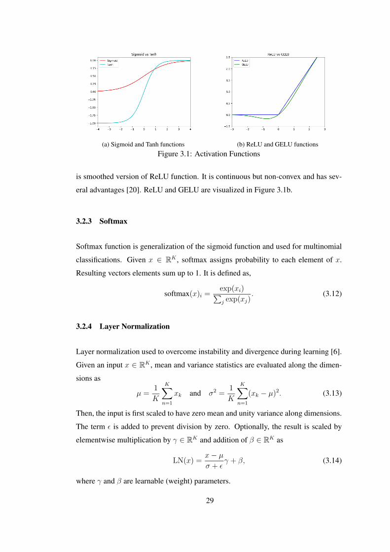
(a) Sigmoid and Tanh functions (b) ReLU and GELU functions

Figure 3.1: Activation Functions

is smoothed version of ReLU function. It is continuous but non-convex and has sev-

eral advantages [20]. ReLU and GELU are visualized in Figure 3.1b.

3.2.3 Softmax

Softmax function is generalization of the sigmoid function and used for multinomial

classifications. Given x ∈ RK , softmax assigns probability to each element of x.

Resulting vectors elements sum up to 1. It is defined as,

softmax(x)i =exp(xi)∑j exp(xj)

. (3.12)

3.2.4 Layer Normalization

Layer normalization used to overcome instability and divergence during learning [6].

Given an input x ∈ RK , mean and variance statistics are evaluated along the dimen-

sions as

µ =1

K

K∑n=1

xk and σ2 =1

K

K∑n=1

(xk − µ)2. (3.13)

Then, the input is first scaled to have zero mean and unity variance along dimensions.

The term ε is added to prevent division by zero. Optionally, the result is scaled by

elementwise multiplication by γ ∈ RK and addition of β ∈ RK as

LN(x) =x− µσ + ε

γ + β, (3.14)

where γ and β are learnable (weight) parameters.

29

3.3 Neural Network Types

3.3.1 Feed Forward Neural Networks (Multilayer Perceptron)

Feed forward neural layers is multidimensional generalization of perceptron. Gen-

erally, a neural layer might output multiple values (say o ∈ R1×do) as vector from

input (say x ∈ R1×dx). Such a setting forces parameter W ∈ Rdx×do to be a ma-

trix. Moreover, activation function is not necessarily a step function. It can be any

nonlinear function like sigmoid, tanh, ReLU etc. Feed Forward Neural Networks

are the generalization of perceptron to approximate any function. Neural layers are

stacked to construct deep feed forward neural network. It defines a nonlinear mapping

y = φ(x; θ) between input x and output y, parametrized by θ that includes (learnable)

parameters like weights, bias and possibly others if defined.

Assuming input signal is x ∈ R1×dx (output of previous layer), activation value of

the layer (h ∈ R1×dh) is calculated by linear transformation (weight W and bias b)

followed by nonlinear activation φ,

h = φ(xW + b), (3.15)

where φ is applied elementwise.

3.3.2 Residual Feed Forward Neural Networks

As Feed Forward Networks becomes deeper, optimizing weights gets difficult. There-

fore, people come with the idea of residual connections [18]. For a fixed number

of stacked layers (usually 2 which is single skip), input and output of the stack is

summed up for next calculations. Replacing feed forward layers with other types

yield different kind of residual network. The difference is demonstrated in Figure 3.2,

where φ corresponds to activation and yellow block means no activation.

30

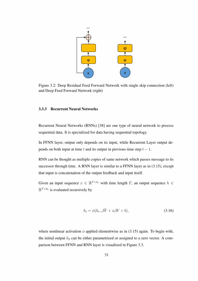
Figure 3.2: Deep Residual Feed Forward Network with single skip connection (left)and Deep Feed Forward Network (right)

3.3.3 Recurrent Neural Networks

Recurrent Neural Networks (RNNs) [38] are one type of neural network to process

sequential data. It is specialized for data having sequential topology.

In FFNN layer, output only depends on its input, while Recurrent Layer output de-

pends on both input at time t and its output in previous time step t− 1.

RNN can be thought as multiple copies of same network which passes message to its

successor through time. A RNN layer is similar to a FFNN layer as in (3.15), except

that input is concatenation of the output feedback and input itself.

Given an input sequence x ∈ RT×dx with time length T , an output sequence h ∈RT×dh is evaluated recursively by

ht = φ(ht−1W + xtW + b), (3.16)

where nonlinear activation φ applied elementwise as in (3.15) again. To begin with,

the initial output h0 can be either parametrized or assigned to a zero vector. A com-

parison between FFNN and RNN layer is visualized in Figure 3.3.

31

Figure 3.3: Feed Forward Layer (left) and Recurrent Layer (right) illustration [31]

Figure 3.4: LSTM Cell [31]

3.3.3.1 Long Short Term Memory

Conventional RNNs have, in general, the problem with vanishing/exploding gradient

[31]. As the sequence gets longer, effect of initial inputs in sequence decreases. This

causes a long term dependence problem. Furthermore, if information from initial

inputs required, gradients either vanish or explode. In order to overcome this problem

another architecture is developed: Long Short Term Memory (LSTM) [22].

LSTM is a special type of RNN. It is explicitly designed to allow learning long-term

dependencies. A single LSTM cell has four neural layers while a vanilla RNN layer

has only one neural layer. In addition to the hidden state ht, there is another state

called cell state Ct. Information flow is controlled by three gates.

Forget Gate controls past memory. According to input, past memory is either kept

32

or forgotten. The sigmoid function (σ) is generally used as an activation function:

ft = σ([ht−1;xt]Wf + bf ). (3.17)

Hyperbolic tangent layer creates new candidate of cell state from the input:

Ct = tanh([ht−1;xt]WC + bC). (3.18)

Input Gate controls contribution from input to cell state (memory):

it = σ([ht−1;xt]Wi + bi). (3.19)

Once what are to be forgotten and added decided, cell state is updated accordingly,

Ct = ft � Ct−1 + it � Ct. (3.20)

using input gate and forget gate outputs. Note that � is elementwise multiplication.

Output Gate controls which part of new cell state to be output:

ot = σ([ht−1;xt]Wo + bo). (3.21)

Finally, cell state is filtered by hyperbolic tangent to push values to be in (−1, 1)

before evaluating the hidden state ht using output gate outputs:

ht = ot � tanh(Ct). (3.22)

3.3.4 Attention Based Networks

As stated earlier, recurrent neural networks are prone to forget long term dependen-

cies. LSTM and other variants are invented to overcome such problems. However,

they cannot attend specific parts of the input. Therefore, researchers come with the

idea of weighted averaging all states through time where weights depends on both

input and output. Let the input sequence x ∈ RT×dx with time length T be encoded

to h ∈ RT×dh . The context vector is calculated using weight the vector α ∈ R1×T

including a scalar for each time step, then attention output is,

Attention(q, h) = αh. (3.23)

33

Attention weight α ∈ RT is calculated using hidden sequence h ∈ RT×dH and query

q ∈ R1×dQ with a predefined a arbitrary function φ depending on choice. Query can

be hidden state itself (self attention) or any input assumed to help attention weighting.

In general form,

α = φ(q, h; θα). (3.24)

3.3.4.1 Transformer

The Transformer was proposed in "Attention is All You Need" [49] paper. Unlike

recurrent networks, this architecture is solely built on attention layers.

A transformer layer consists of feed-forward and attention layers, which makes the

mechanism special. Like RNNs, it can be used as both encoder and decoder. While

encoder layers attend to itself, decoder layers attends both itself and encoded input.

Attention Layer is a mapping from 3 vectors: query Q ∈ RTq×dk , key K ∈ RT×dk

and value V ∈ RT×dv to output, where T is input time length, Tq time length of query,

dk and dv are embedding dimensions. Output is weighted sum of values V through

time dimension while weights are evaluated by compatibility metric of query Q and

key K. In vanilla transformer, compatibility of query and key is evaluated by dot

product, normalizing by√dk. For a query, dot product with all keys are evaluated,

then softmax function is applied to get weights of values,

Attention(Q,K, V ) = softmax

(QKT

√dk

)V. (3.25)

This approach is called Scaled Dot-product Attention.

Instead of performing a single attention, Multi-Head Attention projects keys, queries

and values linearly from dm dimensional vector space to h different spaces using

projection matrices. In this case, attention is performed h times, and results are then

concatenated and linearly projected to final values of the layer. Projection matrices

are model parameters,WQi ∈ Rdm×dk ,WK

i ∈ Rdm×dk ,W Vi ∈ Rdm×dv for i = 1, ..., h.

Also output matrix is used to project multiple values into single one, WO ∈ Rhdv×dm .

34

Figure 3.5: Scaled Dot-Product Attention (left) and Multi-Head Attention (right) [49]

Mathematically,

MHA(Q,K, V ) = Concat(head1, head2, ...headh)WO

headi = Attention(QWQi , KW

Ki , V W

Vi )

. (3.26)

Scaled dot-product attention and Multi-Head attention are demonstrated in Figure 3.5

A transformer layer contains Feed Forward Layer, containing two linear transfor-

mations (W1, b1 and W2, b2) with ReLU-like activation:

FFN(x) = ReLU(xW1 + b1)W2 + b2. (3.27)

Encoder Layer starts with a residual self attention layer. Self attention means that

query, key and value are the same vectors. This is followed by feed forward neural

layer. Both sublayers are employed with resudial connection with layer normaliza-

tion. In other words, summation of layer input and output is passed through layer

normalization:

a =LN(x+ MHA(x, x, x)),

y =LN(a+ FFN(a)).(3.28)

Apart from encoder layers; query, key and value inputs may vary depending on de-

sign. In general,

a =LN(x+ MHA(q, k, v)),

y =LN(a+ FFN(a)).(3.29)

35

Since there are no recurrent or convolutional architecture in the model, sequential

information needs to be embedded. For this purpose, Positional encodings are used.

They have same dimension with as the input x, so that input embeddings can be

added to at the beginning of encoder or decoder stacks. Let the positional encoding

PE ∈ RT×dm . For tth position in time, and ith position in embedding axis (i ∈ N),

PE is defined as follows:

PEt,i =

sin(t/10000i/dm), if i ≡ 0 (mod 2),

cos(t/10000(i−1)/dm), if i ≡ 1 (mod 2),(3.30)

as proposed in the original paper [49].

3.3.4.2 Pre-Layer Normalized Transformer

Original transformer architecture includes layer normalization operations after atten-

tion and feed-forward layers. It is unstable since the values of gradients of output

layers are high. Pre-Layer Normalized Transformer is proposed by [52] by carry-

ing layer normalization operation to in front of attention and feed-forward layers.

Moreover, Parisotto et al. Xiong et al. [33] propose gated transformer which also

includes layer normalizations before attention and feedforward layer. They also state

that although gated architecture improves many reinforcement learning (RL) tasks

drastically, and non-gated pre-layer normalized transformer are also much better than

vanilla transformer.

In pre-layer normalized transformer, encoder equations are:

a =x+ MHA(LN(x),LN(x),LN(x))

y =a+ FFN(LN(a)). (3.31)

A simple pre-layer normalized transformer encoder layer is demonstrated in Fig-

ure 3.6. The difference between post-layer and pre-layer transformer encoders are

also visualized in Figure 3.7

36

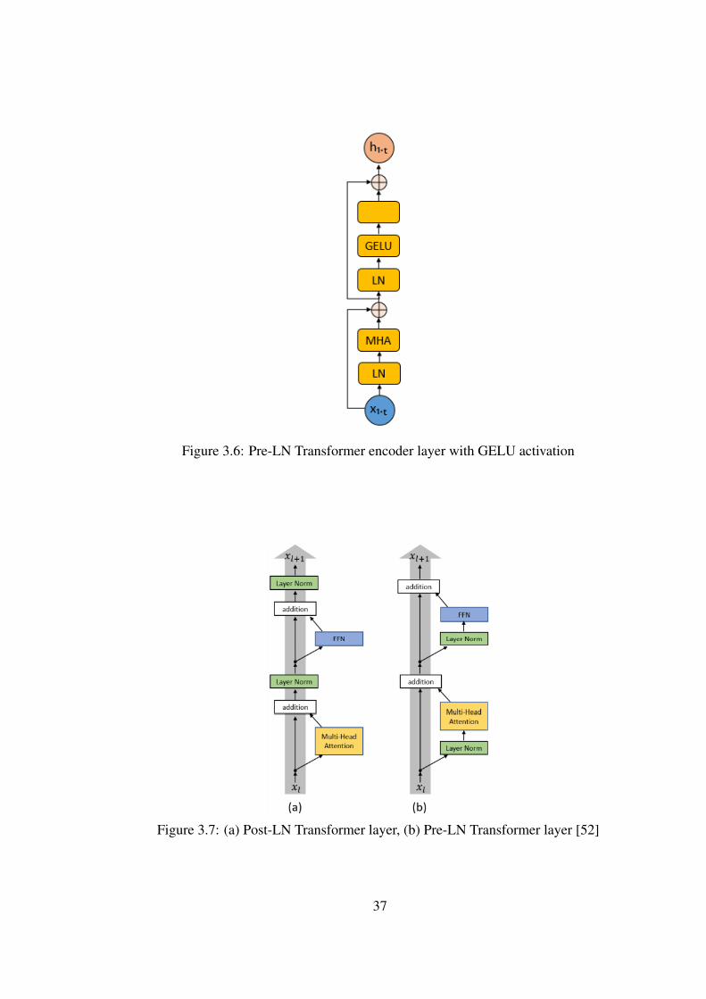
Figure 3.6: Pre-LN Transformer encoder layer with GELU activation

Figure 3.7: (a) Post-LN Transformer layer, (b) Pre-LN Transformer layer [52]

37

38

CHAPTER 4

BIPEDAL WALKING BY TWIN DELAYED DEEP

DETERMINISTIC POLICY GRADIENTS

4.1 Details of the Environment

BipedalWalker-v3 and BipedalWalker-Hardcore-v3 are two simulation environments

of a bipedal robot, with relatively flat course and obstacle course respectively. Dy-

namics of the robot are exactly identical in both environments. Our task is to solve

hardcore version where the agent is expected to learn to run and walk in different road

conditions. Components of the hardcore environment is visualized in Figure 4.1.

The robot has kinematic and lidar sensors, and has deterministic dynamics.

Observation Space contains hull angle, hull angular velocity, hull translational ve-

locities, joint positions, joint angular speeds, leg ground concats and ten lidar rangefinder

measurements. Details and their constraints are summarized in Table 4.1.

The robot has two legs with two joints at knee and hip. Torque is provided to knee

and pelvis joints of both legs. These four torque values forms the Action Space,

presented in Table 4.2 with their constraints.

Reward Function is a bit complex in the sense that the robot should run fast with

little energy while it should not stumble and fall to ground. Directly proportional

to distance traveled forward, +300 points given if agent reaches to end of the path.

However, -10 points (-100 points in the original version) if agent falls, and small

amount of negative reward proportional to absolute value of applied motor torque

τ (to prevent applying unnecessary torque). Lastly, the robots gets negative reward

39

Figure 4.1: Bipedal Walker Hardcore Components [3]

Num Observation Interval0 Hull Angle [−π, π]

1 Hull Angular Speed [−∞,∞]

2 Hull Horizontal Speed [−1, 1]

3 Hull Vertical Speed [−1, 1]

4 Hip 1 Joint Angle [−π, π]

5 Hip 1 Joint Speed [−∞,∞]

6 Knee 1 Joint Angle [−π, π]

7 Knee 1 Joint Speed [−∞,∞]

8 Leg 1 Ground Contact Flag {0, 1}9 Hip 2 Joint Angle [−π, π]

10 Hip 2 Joint Speed [−∞,∞]

11 Knee 2 Joint Angle [−π, π]

12 Knee 2 Joint Speed [−∞,∞]

13 Leg 2 Ground Contact Flag {0, 1}14-23 Lidar measures [−∞,∞]

Table 4.1: Observation Space of Bipedal Walker

40

Num Observation Interval0 Hip 1 Torque [−1, 1]

1 Hip 2 Torque [−1, 1]

2 Knee 1 Torque [−1, 1]

3 Knee 2 Torque [−1, 1]

Table 4.2: Action Space of Bipedal Walker

(a) Perspective (b) Pitfall Behind (c) No Pitfall Behind

Figure 4.2: Perspective of agent and possible realities

propotional to the absolute value of the hull angle θhull for reinforcing to keep the hull

straigth. Mathematically, reward is;

R =

−10, if falls,

130∆x− 5|θhull| − 0.00035|τ |, otherwise.(4.1)

4.1.1 Partial Observability

The environment is partially observable due to following reasons.

• The agent is not able to track behind with the lidar sensor. Unless it has a

memory, it cannot know whether a pitfall or hurdle behind. Illustration is shown

in Figure 4.2.

• There is no accelerometer sensor. Therefore, the agent do not know whether it

is accelerating or decelerating.

In DRL, partial observability is handled by two ways in literature [10]. The first is

incorporating fixed number of last observations while the second way is updating hid-

den belief state using recurrent-like neural network at each time step. Our approach

is somewhere in between. We pass fixed number of past observations into LSTM and

Transformer networks for both actor and critic.

41

4.1.2 Reward Sparsity

Rewards given to the agent is sparse in some circumstances, in the following sense:

• Overcoming big hurdles requires a very specific move. The agent should ex-

plore many actions when faced with a big hurdle.

• Crossing pitfalls also require a specific move but not as complex as big hurdles.

4.1.3 Modifications on Original Envrionment Settings

It is difficult to find an optimal policy directly with available setting. There are few

studies in the literature demonstrating a solution for BipedalWalker-Hardcore-v3. The

following modifications are proposed.

• In original version, agent gets -100 points when its hull hits the floor. In order

to make the robot more greedy, this is changed to -10 points. Otherwise, agent

cannot explore environment since it gets too much punishment when failed and

learns to do nothing.

• Time resolution of simulation is halved (from 50 Hz to 25 Hz) by only observ-

ing last of each two consecutive frames using a custom wrapper function. Since

there is not a high frequency dynamics, this allows nothing but speeding up the

learning process.

• In original implementation, an episode has a time limit. Once this limit is

reached, simulation stops with terminal state flag. On the other hand, when

agent fails before the time limit, the episode ends with terminal state flag too. In

the first case, the terminal state flag causes instability since next step’s value is

not used in value update, since it is not a logical terminal, just time up indicator.

The environment changed such that terminal state flag is not given in this case

unless agent fails.

Once those modifications are applied on the environment, we observed quite improve-

ment on both convergence and scores.

42

(a) Critic Architecture

(b) Actor Architecture

Figure 4.3: Neural Architecture Design

4.2 Proposed Neural Networks

Varying neural backbones are used to encode state information from observations for

both actor and critic networks. In critic network, actions are concatenated by state in-

formation coming from backbones. Then, this concatenated vector is passed through

feed forward layer with hyperbolic tangent activation then through a linear layer with

single output. Before feeding observations to backbone, they are passed through a

linear layer with 96 dimensional output. However, for only LSTM backbones, this

layer is not used and observations are passed to LSTM backbone as it is. In actor

network, backbone is followed by a single layer with tanh activation for action esti-

mation. Again, observations are passed through a linear layer with 96 dimensional

output, and this is not valid for LSTM. Critic and Actor networks are illustrated in

Figure 4.3.

As backbones, following networks are proposed.

43

4.2.1 Residual Feed Forward Network

Incoming vector is passed through 2 layers with 192 dimensional hidden size and 96

dimensional output with single skip connection, where there is GELU activation at

first layer.

4.2.2 Long Short Term Memory

Sequence of incoming vectors is passed though single vanilla LSTM layer with 96

dimensional hidden state. Output at last time step is considered as belief state.

4.2.3 Transformer (Pre-layer Normalized)

Sequence of incoming vectors is passed through single pre-layer normalized trans-

former layer with 192 dimensional feed forward layer with GELU activation after

addition of positional encodings. In multi-head attention, 4 head is used and size of

queries, keys and values are 8 for each head. During multi-head attention, only the

last observation is fed as query so that attentions are calculated only for last state. Its

output is considered as belief state. Note that excluding multi-head attention for this

network gives our residual feed-forward neural network.

4.2.4 Summary of Networks

The designed networks have close number of parameters to make fair comparison

among them. Number of trainable parameters for designed networks are summarized

in Table 4.3.

In addition, we designed transformer network to be same as residual feed forward

network once multi-head attention and preceeding layer normalization is removed. It

can be easily demonstrated by looking at Figure 3.2 (left one, layer normalization is

added in the implementation) and Figure 3.6.

44

Table 4.3: Number of trainable parameters of neural networksNetwork Actor Parameters Critic Parameters

RFFNN 40512 59328LSTM 47616 66432TRSF 52992 71808

4.3 RL Method and Hyperparameters

TD3 and SAC is used as RL algorithm. Hyperparameters are selected by grid search

and best performing values are used. Adam optimizer is used for optimization. For

all models, agents are trained by 8000 episodes.

In TD3, as exploration noise, Ornstein-Uhlenbeck noise is used, and standart devia-

tion is multiplied by 0.9995 at the end of each episode. For LSTM and Transformer,

last 6 observations are used to train agent. More than 6 observations made TD3 algo-

rithm diverge.

In SAC model, squashed gaussian policy is implemented. Therefore, along with layer

giving mean actions, an additive layer is implemented for the standart deviation. For

LSTM and Transformer, last 6 observations and 12 observations are used to train

agent.

All hyperparameters are found after a trial-error process considering the literature.

They are summarized in Table 4.4 and Table 4.5. Training sessions are run by multiple

times to make comparison fair among models since some training sessions fail to

converge and some yield worse results.

4.4 Results

For each episode, episode scores are calculated by summing up rewards of each time

step. In Figure 4.4a and Figure 4.4b, a scatter plot is visualized for each model’s

episode scores. In Figure 4.5a and Figure 4.5b, moving average and standard devia-

45

Table 4.4: Hyperparmeters and Exploration of Learning Processes for TD3```````````````Hyperparameter

ModelRFFNN LSTM Transformer

η (Learning Rate) 4.0× 10−4

β (Momentum) (0.9, 0.999)

γ (Discount Factor) 0.98

Nreplay (Replay Buffer Size) 500000

N (Batch Size) 64

d (Policy Delay) 2

σ (Policy smoothing std) 0.2

τ (Polyak parameter) 0.01

Exploration OU(θ = 4.0, σ = 1.0)

Table 4.5: Hyperparmeters and Exploration of Learning Processes for SAC```````````````Hyperparameter

ModelRFFNN LSTM Transformer

η (Learning Rate) 4.0× 10−4

β (Momentum) (0.9, 0.999)

γ (Discount Factor) 0.98

Nreplay (Replay Buffer Size) 500000

N (Batch Size) 64

τ (Polyak parameter) 0.01

α (Entropy Temperature) 0.01

46

tion is visualized for each model’s episode scores.

(a) TD3 (b) SAC

Figure 4.4: Scatter Plot with Moving Average for Episode Scores (Window length:200 episodes) for SAC

(a) TD3 (b) SAC

Figure 4.5: Moving Average and Standard Deviation for Episode Scores (Windowlength: 200 episodes) for TD3

RFFNN seems enough to make agent walk, although there exist partial observability

in the environment. That model reaches around 221 points in average with TD3 and

245 points with SAC.

Transformer models yield better performance compared to RFFNN. 249 points are

reached by TD3 and 262 points reached by SAC model when 6 last observations are

fed to the model. 266 points are obtained when last 12 observations are fed to model

with SAC.

LSTM model yield the best results by reaching 264 points with TD3 and exceeds 280

points with SAC when 6 last observations are fed to model. 287 points are obtained

when last 12 observations are fed to the model with SAC.

47

Table 4.6: Best checkpoint performances with 100 test simulationsRL Method Model Episode Avg. Score

TD3 RFFNN 6600 207SAC RFFNN 7600 219TD3 TRSF-6 6400 222SAC TRSF-6 6800 254SAC TRSF-12 6000 270TD3 LSTM-6 7000 242SAC LSTM-6 7600 268SAC LSTM-12 7200 298

These scores are maximum obtained average scores of concurrent 200 episodes dur-

ing training. However, while traning, model changes and agent still tries to explore

envrionment. Officially, 300 points in average required in random 100 simulations to

say the environment is solved [4]. Therefore, best checkpoints are evaluated for 100

concurrent simulations without exploration. Results are summarized in Table 4.6.

None of our models exceed 300 point limit, but LSTM-12 model with SAC almost

reaches to the limit Table 4.6. However, all models partially solved problems by

exceeding 200 point limit, while some simulations exceed 300 points with both TD3

(Figure 4.4a) and SAC (Figure 4.4b).

Behaviour of agents are visualized in Figure 4.6, Figure 4.7 and Figure 4.8 for SAC

models. All of 3 models exhibit similar walking characteriscis.

SAC model performes better than TD3 in general, as seen in Figure 4.4a and Fig-

ure 4.4b. In addition, as seen from the moving average points, SAC agents are supe-

rior (Figure 4.5a, Figure 4.5b).

4.5 Discussion

These results are not enough to conclude on a superior neural network for all RL prob-

lems, because there are other factors such as DRL algorithm, number of episodes, net-

work size etc. However, networks are designed to have similar sizes and good model

requires to converge in less episodes. As a result, LSTM is superior to Transformer

48

(a) Stairs

(b) Hurdle

(c) Pitfall

Figure 4.6: Walking Simulation of RFFNN model at best version with SAC

(a) Stairs

(b) Hurdle

(c) Pitfall

Figure 4.7: Walking Simulation of LSTM-12 model at best version with SAC

for our environment. In addition, it is possible to conclude that Transformers can

be an option for partially observed RL problems. Note that this is valid where layer

normalization is applied before multihead attention and feed-forward layers [52] as

opposed to vanilla transformer proposed in [49].

Another result is that incorprating past observations did improve performance signifi-

cantly since environment is partially observable. Especially increasing history length

keeps increasing performance for both LSTM and Transformer models. To address

this issue better, we designed Transformer and RFFNN networks to be almost same

once multi-head attention layer is removed. We observed significant performance

gains as observation history is used as input to controller.

49

(a) Stairs

(b) Hurdle

(c) Pitfall

Figure 4.8: Walking Simulation of Transformer-12 model at best version with SAC

The environment is a difficult one. There are really few available models with solu-

tion [4]. Apart from neural networks, there are other factors affecting performance

such as RL algorithm, rewarding, exploration etc. In this work, all of them are ad-

justed such that the environment becomes solvable. Time frequency is reduced for

sample efficiency and speed. Also, the agent is not informed for the terminal state

when it reaches time limit. Lastly, punishment of falling reduced, so the agent is al-

lowed to learn by mistakes. Those modifications are probably another source of our

high performance.

As RL algorithm, TD3 is selected first, since it is suitable for continuous RL. Ornstein-

Uhlenbeck noise is used for better exploration since it has momentum, and variance

is reduced by time to make agent learn small actions well in later episodes. However,

we cannot feed 12 observation history to sequential models since TD3 failed to learn

in that case. In addition, SAC is used for learning along with TD3. Results are bet-

ter compared to those of TD3. SAC policy maximizes randomness (entropy) if agent

cannot get sufficient reward and this allows the agent to decide where/when to explore

more or less. This way, SAC handles the sparse rewards from the environment better

than TD3.

50

CHAPTER 5

CONCLUSION AND FUTURE WORK

In RL context, learning in a simulation is an important step for mechanical control.

Usually, models are pretrained in simulation environment before learning in reality

due to safety and exploration reasons. Today, RL is rarely used in real world applica-

tions due to safety and sample inefficiency problems.

In this thesis, bipedal robot walking is investigated by deep reinforcement learning

due to complex dynamics in OpenAI Gym’s simulation environment. TD3 and SAC

algorthims are used since they are robust and well suited for continuous control. Also,

environment is slightly modified by reward shaping, halving simulation frequency,

cancelling terminal state information at time limit so that learning becomes easier.

The environment was difficult for exploration. Especially handling big hurdles re-

quires very much exploration. In our results, SAC agents performed better than TD3

since it handles exploration problem by learning how much to explore for a particular

state.

As stated in previous chapters, most of the real world environments are partially ob-

servable. In BipedalWalker-Hardcore-v3, the environment is also partially observable

since agent cannot observe behind and it lacks of acceleration sensors, which is better

to have for controlling mechanical systems. Therefore, we propose to use Long Short

Term Memory (LSTM) and Transformer Neural Networks to capture more informa-

tion from past observations unlike Residual Feed Forward Neural Network (RFFNN)

using a single instant observation as input.

RFFNN model performed well thanks to carefully selected hyperparameters and mod-

51

ifications on the environment. However, sequential models performed much better

indicating partial observability is an important issue for our environment. Among

sequential models, LSTM performed better compared to Transformer agents. How-

ever, note that simple multi-head attention layer added to RFFNN lets Transformer

model emerge. Deciding to use observation history with simple attention layer re-

sulted in significant performance gains. This means that input-output design may be

more important than neural network design.

Another conclusion is that Transformer model performed well enough to say it can

be used in DRL problems. It is surprising because it is not succesfully used in DRL

problems in general except recent architectural developments [33]. In natural lan-

guage processing, this type of attention models completely replace recurrent models

recently, and our results seems promising for this in DRL domain.

Today, all subfields of Deep Learning suffers from lack of analytical methods to de-

sign neural networks. It is mostly based on mathematical & logical intuition. Until

such methods are developed, it seems that we need to try out several neural networks

to get better models, which is the case in our work.

There might be a few possible ways to improve this work. First of all, longer obser-

vation history can be used to handle partial observability for LSTM and Transformer

models. However, this makes learning slower and difficult and requires more stable

RL algorithms and fine tuning on hyperparameters. Secondly, different exploration

strategies might be followed. Especially parameter space exploration [35] may per-

form better since it works better for environments with sparse reward like our envi-

ronment. Lastly, advanced neural networks and RL algorithms (specificly designed

for environment) may be designed by incorprating domain knowledge.

52

REFERENCES

[1] Models for machine learning, https://developer.ibm.com/technologies/artificial-intelligence/articles/cc-models-machine-learning/, Accessed: 2021-09-05, Decem-ber 2017.

[2] BipedalWalker-v2, https://gym.openai.com/envs/BipedalWalker-v2/, Accessed: 2021-09-05, January 2021.

[3] BipedalWalkerHardcore-v2, https://gym.openai.com/envs/BipedalWalkerHardcore-v2/, Accessed: 2021-09-05, January 2021.

[4] OpenAI Gym Leaderboard-v2, https://github.com/openai/gym/wiki/Leaderboard/, Accessed: 2021-09-05, August 2021.

[5] P. Abbeel, A. Coates, M. Quigley, and A. Ng, An Application of ReinforcementLearning to Aerobatic Helicopter Flight, in NIPS, 2006.

[6] J. L. Ba, J. R. Kiros, and G. E. Hinton, Layer Normalization, arXiv:1607.06450[cs, stat], July 2016.

[7] R. Bellman, Dynamic Programming, Dover Publications, Mineola, N.Y, reprintedition edition, March 2003, ISBN 9780486428093.

[8] G. Brockman, V. Cheung, L. Pettersson, J. Schneider, J. Schulman, J. Tang, andW. Zaremba, OpenAI Gym, arXiv:1606.01540 [cs], June 2016.

[9] R. Collobert, K. Kavukcuoglu, and C. Farabet, Torch7: A Matlab-like Environ-ment for Machine Learning, 2011.

[10] G. Dulac-Arnold, D. Mankowitz, and T. Hester, Challenges of Real-World Re-inforcement Learning, arXiv:1904.12901 [cs, stat], April 2019.

[11] V. Francois-Lavet, P. Henderson, R. Islam, M. G. Bellemare, and J. Pineau,An Introduction to Deep Reinforcement Learning, Foundations and Trends® inMachine Learning, 11(3-4), pp. 219–354, 2018, ISSN 1935-8237, 1935-8245.

[12] R. Fris, The Landing of a Quadcopter on Inclined Surfaces using ReinforcementLearning, 2020.

[13] X. Fu, F. Gao, and J. Wu, When Do Drivers Concentrate? Attention-based Driver Behavior Modeling With Deep Reinforcement Learning,arXiv:2002.11385 [cs], June 2020.

53

[14] S. Fujimoto, H. van Hoof, and D. Meger, Addressing Function ApproximationError in Actor-Critic Methods, arXiv:1802.09477 [cs, stat], October 2018.

[15] X. Glorot, A. Bordes, and Y. Bengio, Deep Sparse Rectifier Neural Networks,in Proceedings of the Fourteenth International Conference on Artificial Intelli-gence and Statistics, pp. 315–323, JMLR Workshop and Conference Proceed-ings, June 2011.

[16] T. Haarnoja, S. Ha, A. Zhou, J. Tan, G. Tucker, and S. Levine, Learning to Walkvia Deep Reinforcement Learning, arXiv:1812.11103 [cs, stat], June 2019.

[17] T. Haarnoja, A. Zhou, P. Abbeel, and S. Levine, Soft Actor-Critic: Off-PolicyMaximum Entropy Deep Reinforcement Learning with a Stochastic Actor,arXiv:1801.01290 [cs, stat], August 2018.

[18] K. He, X. Zhang, S. Ren, and J. Sun, Deep Residual Learning for Image Recog-nition, arXiv:1512.03385 [cs], December 2015.

[19] N. Heess, J. J. Hunt, T. P. Lillicrap, and D. Silver, Memory-based control withrecurrent neural networks, arXiv:1512.04455 [cs], December 2015.

[20] D. Hendrycks and K. Gimpel, Gaussian Error Linear Units (GELUs),arXiv:1606.08415 [cs], July 2020.

[21] G. Hinton, Lecture 6e rmsprop: Divide the gradient by a running aver-age of its recent magnitude, http://www.cs.toronto.edu/~tijmen/csc321/slides/lecture_slides_lec6.pdf, Accessed: 2021-09-05, September 2021.

[22] S. Hochreiter and J. Schmidhuber, Long Short-Term Memory, Neural Compu-tation, 9(8), pp. 1735–1780, November 1997, ISSN 0899-7667.

[23] D. P. Kingma and J. Ba, Adam: A Method for Stochastic Optimization,arXiv:1412.6980 [cs], January 2017.

[24] K. Kopsa and A. T. Kutay, Reinforcement learning control for autorotation of asimple point-mass helicopter model, METU, Ankara, 2018.

[25] A. Kumar, N. Paul, and S. N. Omkar, Bipedal Walking Robot using Deep De-terministic Policy Gradient, arXiv:1807.05924 [cs], July 2018.

[26] T. P. Lillicrap, J. J. Hunt, A. Pritzel, N. Heess, T. Erez, Y. Tassa, D. Sil-ver, and D. Wierstra, Continuous control with deep reinforcement learning,arXiv:1509.02971 [cs, stat], July 2019.

[27] W. S. McCulloch and W. Pitts, A logical calculus of the ideas immanent innervous activity, The bulletin of mathematical biophysics, 5(4), pp. 115–133,December 1943, ISSN 1522-9602.

54

[28] T. M. Mitchell, Machine Learning, McGraw-Hill Education, New York, 1st edi-tion edition, March 1997, ISBN 9780070428072.

[29] V. Mnih, K. Kavukcuoglu, D. Silver, A. Graves, I. Antonoglou, D. Wier-stra, and M. Riedmiller, Playing Atari with Deep Reinforcement Learning,arXiv:1312.5602 [cs], December 2013.

[30] V. Mnih, K. Kavukcuoglu, D. Silver, A. A. Rusu, J. Veness, M. G. Bellemare,A. Graves, M. Riedmiller, A. K. Fidjeland, G. Ostrovski, S. Petersen, C. Beat-tie, A. Sadik, I. Antonoglou, H. King, D. Kumaran, D. Wierstra, S. Legg, andD. Hassabis, Human-level control through deep reinforcement learning, Nature,518(7540), pp. 529–533, February 2015, ISSN 1476-4687.

[31] C. Olah, Understanding LSTM Networks – colah’s blog, http://colah.github.io/posts/2015-08-Understanding-LSTMs/, Accessed:2021-09-05, August 2015.

[32] X. Pan, Y. You, Z. Wang, and C. Lu, Virtual to Real Reinforcement Learningfor Autonomous Driving, arXiv:1704.03952 [cs], September 2017.

[33] E. Parisotto, H. F. Song, J. W. Rae, R. Pascanu, C. Gulcehre, S. M. Jayaku-mar, M. Jaderberg, R. L. Kaufman, A. Clark, S. Noury, M. M. Botvinick,N. Heess, and R. Hadsell, Stabilizing Transformers for Reinforcement Learn-ing, arXiv:1910.06764 [cs, stat], October 2019.

[34] A. Paszke, S. Gross, F. Massa, A. Lerer, J. Bradbury, G. Chanan, T. Killeen,Z. Lin, N. Gimelshein, L. Antiga, A. Desmaison, A. Kopf, E. Yang, Z. DeVito,M. Raison, A. Tejani, S. Chilamkurthy, B. Steiner, L. Fang, J. Bai, and S. Chin-tala, PyTorch: An Imperative Style, High-Performance Deep Learning Library,Advances in Neural Information Processing Systems, 32, pp. 8026–8037, 2019.

[35] M. Plappert, R. Houthooft, P. Dhariwal, S. Sidor, R. Y. Chen, X. Chen, T. As-four, P. Abbeel, and M. Andrychowicz, Parameter Space Noise for Exploration,arXiv:1706.01905 [cs, stat], January 2018.

[36] D. Rastogi, Deep Reinforcement Learning for Bipedal Robots, 2017.

[37] F. Rosenblatt, The perceptron: A probabilistic model for information storageand organization in the brain., Psychological Review, 65, pp. 386–408, 1958.

[38] D. E. Rumelhart, G. E. Hinton, and R. J. Williams, Learning representations byback-propagating errors, Nature, 323(6088), pp. 533–536, October 1986, ISSN1476-4687.

[39] S. J. Russell and P. Norvig, Artificial Intelligence A Modern Approach, PrenticeHall, 3 edition, 1995, ISBN 9780136042594.

55

[40] A. E. Sallab, M. Abdou, E. Perot, and S. Yogamani, Deep Reinforcement Learn-ing framework for Autonomous Driving, Electronic Imaging, 2017(19), pp. 70–76, January 2017.

[41] S. R. B. d. Santos, S. N. Givigi, and C. L. N. Júnior, An experimental validationof reinforcement learning applied to the position control of UAVs, in 2012 IEEEInternational Conference on Systems, Man, and Cybernetics (SMC), pp. 2796–2802, October 2012, iSSN: 1062-922X.

[42] S. Shalev-Shwartz, S. Shammah, and A. Shashua, Safe, Multi-Agent, Reinforce-ment Learning for Autonomous Driving, arXiv:1610.03295 [cs, stat], October2016.

[43] D. Silver, G. Lever, N. Heess, T. Degris, D. Wierstra, and M. Riedmiller, Deter-ministic Policy Gradient Algorithms, in International Conference on MachineLearning, pp. 387–395, PMLR, January 2014.

[44] D. R. Song, C. Yang, C. McGreavy, and Z. Li, Recurrent Deterministic Pol-icy Gradient Method for Bipedal Locomotion on Rough Terrain Challenge, in2018 15th International Conference on Control, Automation, Robotics and Vi-sion (ICARCV), pp. 311–318, November 2018.

[45] R. S. Sutton and A. G. Barto, Reinforcement Learning: An Introduction, A Brad-ford Book, February 1998.

[46] G. E. Uhlenbeck and L. S. Ornstein, On the Theory of the Brownian Motion,Physical Review, 36(5), pp. 823–841, September 1930.

[47] U. Upadhyay, N. Shah, S. Ravikanti, and M. Medhe, Transformer Based Rein-forcement Learning For Games, arXiv:1912.03918 [cs], December 2019.

[48] H. van Hasselt, A. Guez, and D. Silver, Deep Reinforcement Learning withDouble Q-learning, arXiv:1509.06461 [cs], December 2015.

[49] A. Vaswani, N. Shazeer, N. Parmar, J. Uszkoreit, L. Jones, A. N. Gomez,L. Kaiser, and I. Polosukhin, Attention is All You Need, 2017.

[50] S. Wang, D. Jia, and X. Weng, Deep Reinforcement Learning for AutonomousDriving, arXiv:1811.11329 [cs], May 2019.

[51] C. J. Watkins and P. Dayan, Technical Note: Q-Learning, Machine Learning,8(3), pp. 279–292, May 1992, ISSN 1573-0565.

[52] R. Xiong, Y. Yang, D. He, K. Zheng, S. Zheng, C. Xing, H. Zhang, Y. Lan,L. Wang, and T.-Y. Liu, On Layer Normalization in the Transformer Architec-ture, arXiv:2002.04745 [cs, stat], June 2020.

56