Biostat Didactic Seminar SeriesBiostat Didactic Seminar Series

Correlation and Regression Correlation and Regression

Part 2Part 2

Robert Boudreau, PhDRobert Boudreau, PhD

Co-Director of Methodology CoreCo-Director of Methodology Core

PITT-Multidisciplinary Clinical Research Center PITT-Multidisciplinary Clinical Research Center

for Rheumatic and Musculoskeletal Diseasesfor Rheumatic and Musculoskeletal Diseases

Core Director for BiostatisticsCore Director for Biostatistics

Center for Aging and Population Health Center for Aging and Population Health

Dept. of Epidemiology, GSPHDept. of Epidemiology, GSPH

Previous Biostat Previous Biostat DidacticsDidactics

Fall 2009 – Spring 2010 Fall 2009 – Spring 2010 1.1. Descriptive Statistics: Examining Your Data Descriptive Statistics: Examining Your Data Data types: Qualitative (Categorical), Ordinal, QuantitativeData types: Qualitative (Categorical), Ordinal, Quantitative Mean, SD, medians, quartiles, IQR, skewness, histograms, Mean, SD, medians, quartiles, IQR, skewness, histograms,

boxplotsboxplots

2.2. Group Comparisons: Part 1Group Comparisons: Part 1 Normal dist (mean, SD: 68%, 95%, 99% Normal dist (mean, SD: 68%, 95%, 99%

interpretation)interpretation) t-dist, degrees of freedom (n-1)t-dist, degrees of freedom (n-1) Confidence interval for the meanConfidence interval for the mean

3.3. Group Comparisons: Part 2Group Comparisons: Part 2 Comparing means: Two-sample independent t-testComparing means: Two-sample independent t-test

pooled and unequal variance (Satterthwaite) versionspooled and unequal variance (Satterthwaite) versions interpretation of p-values, type I (false positive) and type II interpretation of p-values, type I (false positive) and type II

errorerror

Previous Biostat Previous Biostat DidacticsDidactics

Fall 2009 – Spring 2010 Fall 2009 – Spring 2010 4.4. Group Comparisons Part 3: Nonparametric Group Comparisons Part 3: Nonparametric Tests, Tests,

Chi-squares and Fisher ExactChi-squares and Fisher Exact Comparing groups having small sample sizes (< Comparing groups having small sample sizes (<

20) or with non-normal distributions20) or with non-normal distributions

=> Use Wilcoxon Rank-Sum Test (nonparametric)=> Use Wilcoxon Rank-Sum Test (nonparametric)

(based on rank-order when sorted rather than(based on rank-order when sorted rather than

on actual numeric values)on actual numeric values) Comparing groups in the % falling into diff Comparing groups in the % falling into diff

categoriescategories

=> Use Chi-square, Fisher’s Exact (if any cell n => Use Chi-square, Fisher’s Exact (if any cell n < 5)< 5)

Previous Biostat Previous Biostat DidacticsDidactics

Fall 2009 – Spring 2010 Fall 2009 – Spring 2010 5.5. Correlation, Regression and Covariate-Correlation, Regression and Covariate-Adjusted Group Comparisons Adjusted Group Comparisons

Pearson vs Spearman correlation Pearson vs Spearman correlation

=> linear vs monotone association => linear vs monotone association Regression: Regression: interpretation of beta coefficients interpretation of beta coefficients

Standard errors, p-valuesStandard errors, p-values Continuous predictor => beta coeff is a slopeContinuous predictor => beta coeff is a slope Dichotomous (e.g. group “dummy” 0,1 valued variable)Dichotomous (e.g. group “dummy” 0,1 valued variable)

=> beta coeff is difference in response vs “referent” => beta coeff is difference in response vs “referent”

treatment_group = 1treatment_group = 1 knockout mouseknockout mouse

= 0= 0 wild mouse (referent) wild mouse (referent) Adjusting for important covars when comparing Adjusting for important covars when comparing

groups groups

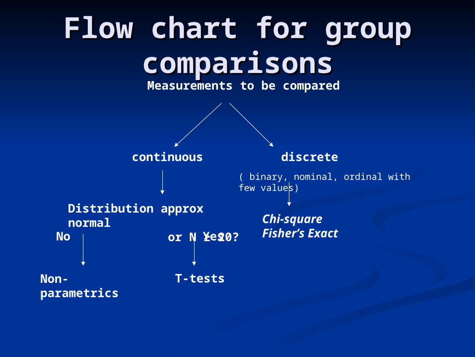
Flow chart for group Flow chart for group comparisonscomparisons

Measurements to be compared

continuous

Distribution approx normal or N ≥ 20?

No Yes

Non-parametrics T-tests

discrete

( binary, nominal, ordinal with few values)

Chi-squareFisher’s Exact

Flow chart for regression Flow chart for regression modelsmodels

(includes adjusted group comparisons)(includes adjusted group comparisons)Outcome variable continuous or dichotomous?

dichotomouscontinuous

Time-to-event available (or relevant)?

No Yes

Multiple logistic regression

Cox proportionalhazards regression

Predictor variable categorical?

No Yes(e.g. groups)

Multiple linear regression

ANCOVA(Multiple linear regression -using dummyvariable(s) forcategorical var(s)

Analysis From Last Analysis From Last Didactic …Didactic …

In Health, Aging and Body Composition Knee-OA Substudy:In Health, Aging and Body Composition Knee-OA Substudy:

Examine Association between SxRxKOA (knee OA) and CRP Examine Association between SxRxKOA (knee OA) and CRP adjusted for BMI.adjusted for BMI.

Motivation:Motivation: Sowers M, Hochberg M et. al. C-reactive protein as a biomarker

of emergent osteoarthritis. Osteoarthritis and CartilageVolume 10, Issue 8, August 2002, Pages 595-601

Conclusion: “CRP is highly associated with Knee OA; however, its high correlation with obesity limits its utility as an exclusive marker for knee OA”

All White Females in HABC (N=844)[includes SxRxKOA (n=93); also rest of parent study cohort]

N=5N=5 had CRP > 30 (max=63.2)

log CRP

White FemalesWhite Females

Difference in average logCRP: 0.76 – 0.43 = 0.33

Knee OA

P-value

No (n=752) Yes (n=92)

Mean (SD) Mean (SD)

Equal vars Unequal

logCRP 0.43 (0.83) 0.76 (0.58) 0.0002 < 0.0001

BMI 25.4 (4.3) 28.8 (5.2) < 0.0001 < 0.0001

logCRP SD’s were signif diff (p<0.0001) => Use Satterthwaite unequal variance test

Two-Group Unadjusted Two-Group Unadjusted Comparison Comparison

Of Means Using Regression Of Means Using Regression with Dummy-coded Groupswith Dummy-coded Groups

* No OA is “referent” group (i.e. kneeOA=0)

HABCID logCRP kneeOA BMI

1000 1.10972 0 22.5922 1001 0.16526 0 22.2751 1002 1.50988 0 26.1207 1003 -0.62048 0 26.9536 1014 0.65657 1 26.5266 1017 0.82039 1 30.2526 1033 0.84323 1 29.8458 1048 1.67787 1 39.8597

proc reg data=kneeOA_vs_noOA; model logCRP= KneeOA; where female=1 and white=1;run;

White Females: 2-Group White Females: 2-Group Comparison Using Dummy-Comparison Using Dummy-

coded Groupscoded Groups* No OA is “referent” group (KneeOA=0);

proc reg data=kneeOA_vs_noOA; model logCRP= KneeOA; where female=1 and white=1;run;

Note: Regression using Dummy (0, 1) for group variable (e.g. KneeOA=0,1) In regression, equal (pooled) variance is assumed

“No OA” mean

“kneeOA” mean difference from referent

Same p-value as equalvariance t-test

Model: logCRP=0.42682 + 0.33091*kneeOA (intercept) KneeOA=0 logCRP=0.42682+0.33091*0 = 0.42682

KneeOA=1 logCRP=0.42682+0.33091*1 = 0.75773

proc reg data=kneeOA_vs_noOA; model logCRP= KneeOA; where female=1 and white=1;run;

ANCOVA (Analysis of ANCOVA (Analysis of Covariance)Covariance)

Compare logCRP adjusted Compare logCRP adjusted for BMIfor BMI

ANCOVA (Analysis of ANCOVA (Analysis of Covariance)Covariance)

Compare logCRP adjusted Compare logCRP adjusted for BMIfor BMIproc reg data=kneeOA_vs_noOA;

model logCRP=KneeOA bmi; where female=1 and white=1;run;

Note: Equal BMI slopes in each group is being modeled

Unadjusted diffWas 0.33

BMI partially“explains” thisdifference

{

UnadjustedMean Difference

Notice: At any BMI level, the mean logCRP differencebetween KneeOA vs Notis smaller than the unadjusted difference

logCRP between KneeOA vs logCRP between KneeOA vs NotNot

Adjusted for BMI, AgeAdjusted for BMI, Ageand Anti-inflammatory Medsand Anti-inflammatory Meds

Note: age is not significant

(caveat: narrow HABC study age range: 69-80)

White Females: 2-Group White Females: 2-Group Comparison Using Dummy-Comparison Using Dummy-

coded Groupscoded Groups* No OA is “referent” group (KneeOA=0);

proc reg data=kneeOA_vs_noOA; model logCRP= KneeOA; where female=1 and white=1;run;

Note: Regression using Dummy (0, 1) for group variable (e.g. KneeOA=0,1) In regression, equal (pooled) variance is assumed

“No OA” mean

“kneeOA” mean difference from referent

Pearson CorrelationPearson CorrelationPearson Correlation = a measure of linear association

Pearson vs Spearman Pearson vs Spearman CorrelationCorrelation

Spearman: • A measure of rank order correlation • Works for any general trend that is increasing or decreasing and not necessarily linear

Pearson vs Spearman Pearson vs Spearman CorrelationCorrelation

Spearman: • A measure of rank order correlation

• Works for any general trend that is increasing or decreasing and not necessarily linear

• Equals Pearson Correlation using the ranks of the observations instead of actual values

Heuristically: Spearman measures degree that

low goes with low, middle with middle, high with high

Effect of Centering BMI at Effect of Centering BMI at 2525

proc reg data=kneeOA_vs_noOA; model logCRP=bmi_minus25; where female=1 and white=1 and kneeOA=1;run;

logCRP= 0.58144 + 0.04699*(BMI-25) = 0.58144 at BMI=25 (see graphic)

Effect of Centering BMI Effect of Centering BMI at 25at 25

Model 2: logCRP= 0.58144 + 0.04699*(BMI-25) = 0.58144-25*0.04699 + 0.04699*BMI =-0.59337 + 0.04699*BMI

{

UnadjustedMean Difference

ANCOVA (Analysis of ANCOVA (Analysis of Covariance)Covariance)

Centering BMI at 25Centering BMI at 25proc reg data=kneeOA_vs_noOA; model logCRP=KneeOA bmi_minus25; where female=1 and white=1;run;

Note: Equal BMI slopes in each group is being modeled

Check of ANCOVA Assumption: Check of ANCOVA Assumption:

Equality of BMI slopes: KneeOA vs Equality of BMI slopes: KneeOA vs NotNotproc reg data=knee_vs_noOA;proc reg data=knee_vs_noOA;

model logCRP=KneeOA bmi BMI_x_KneeOA;model logCRP=KneeOA bmi BMI_x_KneeOA; where female=1 and white=1;where female=1 and white=1;run;run; (“interaction term”)(“interaction term”)

HABCID logCRP kneeOA BMI BMI_x_KneeOA

1000 1.10972 0 22.5922 0.0000 1001 0.16526 0 22.2751 0.0000 1002 1.50988 0 26.1207 0.0000 1003 -0.62048 0 26.9536 0.0000 1014 0.65657 1 26.5266 26.5266 1017 0.82039 1 30.2526 30.2526 1033 0.84323 1 29.8458 29.8458 1048 1.67787 1 39.8597 39.8597

Check of ANCOVA Assumption: Check of ANCOVA Assumption:

Equality of BMI slopes: KneeOA vs Equality of BMI slopes: KneeOA vs NotNotproc reg data=knee_vs_noOA;proc reg data=knee_vs_noOA;

model logCRP=KneeOA bmi BMI_x_KneeOA;model logCRP=KneeOA bmi BMI_x_KneeOA;

where female=1 and white=1;where female=1 and white=1;

run;run;

The “BMI” slopes are not signif different (p=0.8019) => they are parallel

Thank youThank you

Questions, comments, suggestions or insights?Questions, comments, suggestions or insights?

Remaining time: Open consultation …Remaining time: Open consultation …