BIOMECHANICAL RESPONSE OF THE ANKLE TO EXCESSIVE EXTERNAL ROTATION …2694/... · ·...

BIOMECHANICAL RESPONSE OF THE ANKLE TO

EXCESSIVE EXTERNAL ROTATION

By

Keith D. Button

A DISSERTATION

Submitted to

Michigan State University

in partial fulfillment of the requirements

for the degree of

Engineering Mechanics-Doctor of Philosophy

2015

ABSTRACT

BIOMECHANICAL RESPONSE OF THE ANKLE TO EXCESSIVE EXTERNAL

ROTATION

By

Keith D. Button

Acute ankle damage is one of the most commonly observed athletic injuries, accounting for 10-

30% of sports-related injuries in young athletes. Most frequently, damage occurs to the lateral

ligamentous complex, involving the anterior talofibular ligament and calcaneofibular ligament.

Medial ankle injuries involve damage to the anterior deltoid ligament, while syndesmotic (or

high) ankle injuries are defined as damage to the anterior tibiofibular ligament. While less

common than lateral ankle injuries, both medial and high ankle injuries are of particular interest

to researchers due to their longer recovery time and potential for long-term ankle dysfunction.

While combinations of eversion, dorsiflexion, and external rotation are often implicated in

medial and high ankle sprains, the exact mechanisms are still unclear. Additionally, although

studies have investigated the effect of shoe-surface interface on injury risk, few researchers have

examined the effect of shoe rotational stiffness on motion of the ankle, torque generated, and

subsequent injury location and severity during external rotation. One hypothesis of this

dissertation was that the motion of the ankle joint and the location of injury during external

rotation are functions of both the position of the ankle prior to rotation and the amount of

constraint on the ankle. A second hypothesis was that specimen-specific, rigid body modeling

could be utilized to simulate injury-level ankle rotation in addition to modeling the effect of

different footwear on motion of the ankle. Computational modeling, in addition to cadaveric and

in vivo human subject testing was utilized to test these hypotheses.

Specimen-specific computational models simulating injuries observed experimentally revealed

that external foot rotation primarily strains the medial ankle ligaments, but pre-everting the

ankles prior to rotation puts the primary strain on the syndesmotic ankle ligaments. Additionally,

there was a significant difference in the amount of strain in simulations modelling complete

ruptures versus partial tears. A follow-up study involving the measurement of cadaver joint

kinematics during external foot rotation concluded there was significantly more talocrural joint

rotation, but significantly less subtalar joint rotation in a neutral versus pre-everted ankle,

potentially explaining the location of injury during external rotation. In a separate cadaver study

investigating the effect of foot constraint, ankles constrained by a ‘stiff’ football shoe

experienced more ankle joint rotation, but less eversion than ankles constrained by a more

‘flexible’ shoe. As a result, ankles in stiff shoes experienced combination syndesmotic and

medial ankle injuries in addition to high strains in these ligaments. Ankles in flexible shoes saw

less combination injuries, but higher strains in the subtalar ligaments. This effect of ankle

constraint on joint motion was then quantified by measuring joint kinematics in human subjects,

and computational modelling provided an estimation of injury risk as a function of foot rotation

and constraint. A final human subject study involved calculating the stiffness of the

unconstrained ankle joint during voluntary external foot rotation in order to more accurately

model the ankle in the future. The information from these studies may aid in the implementation

of preventative measures in order to mitigate the risk of future ankle injury resulting from

excessive levels of external rotation.

iv

Thank you Mom, Dad, Rachael, and Erin. You are my heroes and your support means

everything.

v

ACKNOWLEDGEMENTS

I would like to thank my mentor, Dr. Roger C. Haut, for his support, expertise, and leadership

throughout my research at the Orthopaedic Biomechanics Laboratories (OBL). I would like to

acknowledge Dr. Dashin Liu, Dr. Eric Meyer, Dr. John Powell, Dr. Feng Wei, and Dr. Neil

Wright for their insight when serving on my committee. I would also like to thank Mr. Jerrod

Braman for his expertise in gait analysis, Mr. Cliff Beckett for his technical assistance, Mrs. Jean

Atkinson for help with specimen preparation, and Dr. Maureen Schaefer for clinical advice. I

would like to thank my co-investigators at Colorado State University: Garrett Coatney, Dr.

Tammy Haut Donahue, Kristine Fischenich, Hannah Pauly, and Benjamin Wheatley. I would

lastly like to thank all my coworkers in the OBL for their help and friendship: Benjamin

Carruthers, Mark Davison, Trevor Deland, Kathleen Fitzsimons, Mike Klein, Katie Landwehr,

Kevin Leikert, Patrick Vaughn, and Brian Weaver.

vi

TABLE OF CONTENTS

LIST OF TABLES ......................................................................................................................... ix

LIST OF FIGURES .........................................................................................................................x

CHAPTER 1: INTRODUCTION AND BACKGROUND .............................................................1

Ankle Anatomy and Kinematics ..........................................................................................1

Ankle Injury in Sports ..........................................................................................................3

Inversion Injuries .....................................................................................................4

External Rotation Injuries ........................................................................................4

Risk Factors for External Rotation Injuries .........................................................................6

Shoe Surface Interface .............................................................................................6

Shoe Stiffness...........................................................................................................7

Computational Modelling ....................................................................................................8

Summary and Objectives .....................................................................................................9

CHAPTER 2: SPECIMEN-SPECIFIC COMPUTATIONAL MODELS OF ANKLE

SPRAINS PRODUCED IN A LABORATORY SETTING .............................................11

ABSTRACT .......................................................................................................................11

INTRODUCTION .............................................................................................................13

METHODS ........................................................................................................................15

Cadaver Experiment...............................................................................................15

Model Development...............................................................................................17

Simulation ..............................................................................................................19

RESULTS ..........................................................................................................................20

DISCUSSION ....................................................................................................................26

CHAPTER 3: EFFECT OF PRE-EVERSION ON TALOCRURAL AND SUBTALAR

JOINT MOTION DURING ANKLE EXTERNAL ROTATION ....................................31

ABSTRACT .......................................................................................................................31

INTRODUCTION .............................................................................................................32

METHODS ........................................................................................................................33

RESULTS ..........................................................................................................................36

DISCUSSION ....................................................................................................................37

vii

CHAPTER 4: ROTATIONAL STIFFNESS OF AMERICAN FOOTBALL SHOES AFFECTS

ANKLE BIOMECHANICS AND INJURY SEVERITY .................................................42

ABSTRACT .......................................................................................................................42

INTRODUCTION .............................................................................................................43

METHODS ........................................................................................................................46

Shoe Selection ........................................................................................................46

Cadaver Tests .........................................................................................................47

Motion Analysis .....................................................................................................51

Computational Modelling ......................................................................................52

Statistical Analysis .................................................................................................52

RESULTS ..........................................................................................................................53

Experimental ..........................................................................................................53


DISCUSSION ....................................................................................................................59

CHAPTER 5: THE EFFECT OF ROTATIONAL STIFFNESS ON ANKLE JOINT MOTION

AND LIGAMENT STRAIN DURING EXTERNAL ROTATION .....................65

ABSTRACT .......................................................................................................................65

INTRODUCTION .............................................................................................................66

METHODS ........................................................................................................................69

Tape Stiffness Tests ...............................................................................................69

Human Subject Tests .............................................................................................71


Statistical Analysis .................................................................................................76

RESULTS ..........................................................................................................................76

DISCUSSION ....................................................................................................................82

CHAPTER 6: A METHOD OF DETERMINING IN VIVO DYNAMIC HUMAN

ANKLE STIFFNESS DURING EXTERNAL ROTATION .............................................87

ABSTRACT .......................................................................................................................87

INTRODUCTION .............................................................................................................87

METHODS ........................................................................................................................89

RESULTS ..........................................................................................................................93

DISCUSSION ....................................................................................................................93

viii

CHAPTER 7: CONCLUSIONS ...................................................................................................97

Overview ............................................................................................................................97

Chapter 2 ............................................................................................................................98

Chapter 3 ............................................................................................................................99

Chapter 4 ..........................................................................................................................100

Chapter 5 ..........................................................................................................................102

Chapter 6 ..........................................................................................................................104

Contributions to the Literature .........................................................................................106

Influence of shoe design on ankle movement and injury ...................................106

Determination of failure-level ligament strains ..................................................106

Use of specimen-specific computational models ................................................107

APPENDICES .............................................................................................................................108

RESEARCH PUBLICATIONS .......................................................................................109

SOP (Standard Operating Procedure) for Building Specimen-Specific Computational

Ankle Models ...................................................................................................................112

SOP (Standard Operating Procedure) For Calculating Ankle Joint Motion Given Vicon

Data ..................................................................................................................................118

REFERENCES ............................................................................................................................132

ix

LIST OF TABLES

Table 2-1 Results of the cadaver experiment for the neutral and everted ankle ...........................25

Table 2-2 Comparison of the talus external rotations with respect to the tibia (deg) from the

cadaver study with the computational talus rotations ..................................................................25

Table 3-1 Motions of the subtalar and talocrural joint for 20 degrees of external rotation ........37

Table 4-1 Lateral (a), posterior (b), and medial (c) views of one of the specimen-specific models

in SolidWorks with linear springs representing ligaments. ...........................................................54

Table 4-2 Strains at failure rotation for the anterior tibiofibular ligament (ATiFL), anterior

tibiotalar ligament (ATiTL), posterior tibiotalar ligament (PTiTL), interosseous talocalcaneal

ligament (ITaCL), lateral talocalcaneal ligament (LTaCL), medial talocalcaneal ligament

(MTaCL), and posterior talocalcaneal ligament (PTaCL). (Underlining represents ligaments

that ruptured or avulsed) ...............................................................................................................55

Table 6-1 Ankle stiffnesses in three directions obtained from subjects performing a single legged

external rotation of the foot with standard deviations in parenthesis. Note: the absolute value of

the inversion-eversion slope was taken so that the reported number was positive. ......................92

Table 6-2 Stiffness values from previous studies ...........................................................................94

Table 7-1 Motions of the subtalar and talocrural joint for 20 degrees of external rotation .......100

Table 7-2 Summary of injury mechanisms and failure metrics from cadaver experiment ..........101

Table 7-3 Ankle stiffness in three directions obtained from subjects performing a single legged

external rotation of the foot. . .....................................................................................................105

Table A-1 Raw Data from Cadaver Failure Tests (Chapter 4) ...................................................124

Table A-2 Raw Data from Tape Stiffness Tests (Chapter 5) .......................................................127

Table A-3 Input Motions for Computational Model (Chapter 5) ................................................128

x

LIST OF FIGURES

Figure 1-1 Medial view of the bony anatomy of the ankle ..............................................................1

Figure 1-2 Lateral (left) and medial (right) view of the osteoligamentous ankle anatomy ............2

Figure 1-3 The three motions of the ankle illustrated about a Cartesian coordinate system .........3

Figure 2-1 Setup for the cadaver experiment by Wei et al. ............................................................16

Figure 2-2 The cadaver taping pattern (a) and the model taping pattern represented by springs

(b). Note: for clarity all ligament springs and the plate springs on the medial side of the ankle

were set invisible. ...........................................................................................................................18

Figure 2-3 Injury mechanisms reported from the cadaver study by Wei et al. (Wei et al., 2012b).

Partial tear of the ATiFL (a); Rupture of the ATiFL (b); Partial tear of the ATiTL (c); Rupture

of the ATiTL (d); Tibial avulsion of the ATiTL (e); Partial tear of the TiNL(f). Note: the location

of injury is shown with a hemostat. ................................................................................................21

Figure 2-4 Ligaments with average model predicted strains greater than 2% for the neutral case

in 3 of 4 cases in which ligament injury occurred .........................................................................22

Figure 2-5 Strains in the ATiFL and the two deltoid ligaments (ATiTL and TiNL) for the neutral

case for each specimen modeled ....................................................................................................23

Figure 2-6 Ligaments with average model predicted strains greater than 2% for the everted

simulations .....................................................................................................................................24

Figure 2-7 Strains in the ATiFL and the two deltoid ligaments (ATiTL and TiNL) for the everted

simulations .....................................................................................................................................24

Figure 3-1 Cadaver foot taped to a polycarbonate plate (a). Ankle with reflective marker array

in the tibia, talus, and calcaneus in the testing fixture (b). ............................................................34

Figure 3-2 Orthogonal coordinate axes on the tibia, talus, and calcaneus. .................................36

Figure 3-3 The sustentaculum tali of the calcaneus locks with the articulating surface of the talus

in a neutral position shown from the posterior (a) and medial (b) view. When everted, these

surfaces unlock, shown in the posterior (c) and medial (d) view. ................................................40

Figure 4-1 Posterior view of a neutral (left) and everted foot (right). .........................................44

Figure 4-2 Football shoes used for the current study: Nike Flyposite (a) and Nike Zoom Air (b).

........................................................................................................................................................47

Figure 4-3 Football cleat mold made of epoxy resin used to fix the shoe to the testing fixture ....48

xi

Figure 4-4 The experiments were performed on a biaxial testing machine with the motions of the

talus and tibia tracked by a 5-camera motion capture system. .....................................................50

Figure 4-5 An example of the torque data from a sub-failure (a) and a failure (b) test. The

failure occurs when there is a steep drop in torque, as indicated by the arrow. ...........................50

Figure 4-6 Lateral (a), posterior (b), and medial (c) views of one of the specimen-specific models

in SolidWorks with linear springs representing ligaments. ...........................................................51

Figure 4-7 Fibular fracture (a), medial malleolus fracture (b), ATiFL avulsion (c), ATiTL

avulsion (d), ATiFL tear (e), and ATiTL tear (f)............................................................................57

Figure 4-8 Representative plot of the ATiFL and ATiTL strains versus tibia rotation in a

simulation of the combination ATiFL and ATiTL injury scenario (specimen 2, stiff shoe). ..........58

Figure 5-1 The surrogate ankle taped to the polycarbonate plate using Elastikon (a), PowerFlex

(b), and Sher-Light (c). ..................................................................................................................69

Figure 5-2 The surrogate limb was attached to the testing machine .............................................70

Figure 5-3 Marker arrays were placed on the subject’s anterior tibia, about 10 cm distal to the

patella, and the calcaneal tuberosity. ............................................................................................72

Figure 5-4 Three orthogonal axes of the ankle. Rotations about these axes are described as

plantarflexion/dorsiflexion, eversion/inversion, and internal/external rotation. ..........................74

Figure 5-5 Torque-rotation curves for the three tape designs and two shoe designs from

rotational stiffness tests (a), and rotational stiffness values determined from the slopes of the

torque-rotation curves (b). Curves with different symbols (* # ƚ ¥) indicate statistically different

stiffness between designs................................................................................................................77

Figure 5-6 Mean ankle joint dorsiflexion-tibia rotation curves for the three tape (and no-tape)

designs from an in vivo external foot rotation (n=6). There were no significant differences

between tape designs......................................................................................................................78



between tape designs. ...................................................................................................................78

Figure 5-8 Mean ankle joint eversion-tibia rotation curves for the three tape (and no-tape)

designs from an in vivo external foot rotation (n=6). Different symbols (* #) indicate

statistically different curves. ..........................................................................................................79

xii

Figure 5-9 Predicted anterior tibiofibular ligament (ATiFL) (a) and anterior tibiotalar ligament

(ATiTL) (b) strain versus tibia rotation for an ankle constrained with tape stiffness ranging from

0 to 30 Nm/deg. Inputs for ankle joint motion were based on predictive equations 3a-3c. .........81

Figure 6-1 Marker set of the Oxford Foot Model (Carson et al., 2001). The subjects stood on

one foot and performed an internal rotation of the body (external rotation of the foot). ..............89

Figure 6-2 Sample of a moment versus time plot (left) and rotation versus time plot (right) for all

three movements: internal-external rotation, inversion-eversion, and plantarflexion-dorsiflexion.

Data from the loading phase (shaded in the figure) for moment vs. time were extracted and

plotted against the extracted rotation vs. time data, as shown in Figure 6-3................................90

Figure 6-3 Samples of moment versus rotation plots in the loading phase for internal-external

rotation (left), inversion-eversion (right), and plantarflexion-dorsiflexion (bottom). ...................91

Figure 7-1 Strains in the ATiFL and two deltoid ligaments (ATiTL and TiNL) for neutral and

everted simulations. .....................................................................................................................98

Figure 7-2 Representative plot of the ATiFL and ATiTL strains versus tibia rotation ................101

Figure 7-3 Mean ankle joint dorsiflexion, external rotation, and eversion vs. tibia rotation for

three tapes and a tapeless condition. ..........................................................................................103



0 to 30 Nm/deg. Inputs for ankle joint motion were based on predictive equations 3a-3c. .......104

Figure A-1 Typical MIMICS interface ........................................................................................112

Figure A-2 Orthogonal coordinate axes on the tibia, talus, and calcaneus. ...............................118

Figure A-3 Marker arrays in a cadaver ankle (a) and human subject (b) ..................................119

1

CHAPTER 1:

INTRODUCTION AND BACKGROUND

Ankle Anatomy and Kinematics

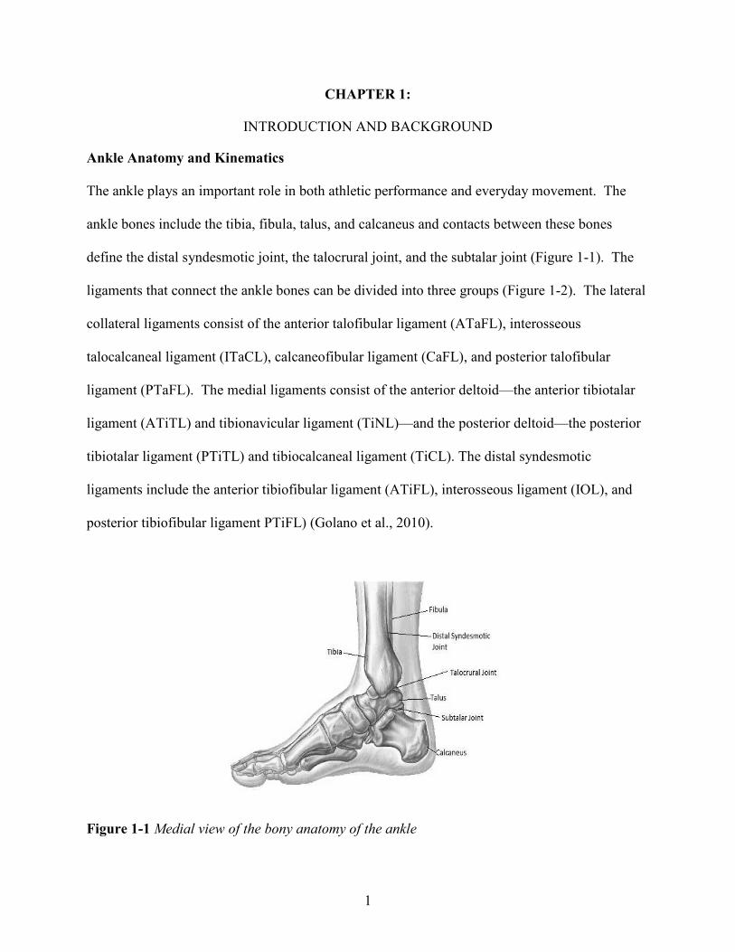
The ankle plays an important role in both athletic performance and everyday movement. The

ankle bones include the tibia, fibula, talus, and calcaneus and contacts between these bones

define the distal syndesmotic joint, the talocrural joint, and the subtalar joint (Figure 1-1). The

ligaments that connect the ankle bones can be divided into three groups (Figure 1-2). The lateral

collateral ligaments consist of the anterior talofibular ligament (ATaFL), interosseous

talocalcaneal ligament (ITaCL), calcaneofibular ligament (CaFL), and posterior talofibular

ligament (PTaFL). The medial ligaments consist of the anterior deltoid—the anterior tibiotalar

ligament (ATiTL) and tibionavicular ligament (TiNL)—and the posterior deltoid—the posterior

tibiotalar ligament (PTiTL) and tibiocalcaneal ligament (TiCL). The distal syndesmotic

ligaments include the anterior tibiofibular ligament (ATiFL), interosseous ligament (IOL), and

posterior tibiofibular ligament PTiFL) (Golano et al., 2010).

Figure 1-1 Medial view of the bony anatomy of the ankle

2

Figure 1-2 Lateral (left) and medial (right) view of the osteoligamentous ankle anatomy

Motion of the ankle is complex and involves coupled motion across three axes (Figure 1-3).

Rotation about the y-axis (medial-lateral) is called plantarflexion when the toes rotate away from

the body and dorsiflexion when the toes rotate towards the body. Rotation about the x-axis (long

axis) is called eversion when the bottom of the foot faces away from the body center and

inversion when the bottom of the foot points towards the body center. Rotation about the z-axis

(inferior-superior) is called internal rotation when the long axis points towards body center and

external rotation when the long axis points away from the body center. Motion of the talocrural

joint is primarily responsible for plantarflexion/dorsiflexion and internal/external rotation while

motion of the subtalar joint is primarily responsible for inversion/eversion.

Motion of the ankle rarely isolates one of these three rotations, resulting in coupled motions due

to the bony and ligamentous constraints of the ankle. Eversion and external rotation are strongly

coupled and both weakly coupled with dorsiflexion. Inversion and internal rotation are also

3

strongly coupled and weakly coupled with plantarflexion. Forced rotation about one axis usually

results in a ‘transferal of rotation’ in which rotations occur about the other axes in order to

dissipate torsion (Hicks, 1953, Lundberg et al., 1989b). When this natural response of the ankle

is compromised by restricting movement about one or more axes, increased strain is generated in

ligaments or bones resulting in injury.

Figure 1-3 The three motions of the ankle illustrated about a Cartesian coordinate system

Ankle Injury in Sports

Damage to the ankle is the most frequently observed injury in the emergency room (Boruta et al.,

1990) and accounts for 10-30% of all sports injuries (Waterman et al., 2010). In some sports,

these percentages can be even higher: Garrick and Requa report that the rate could be as high as

74% in softball, 76% in racquet sports and football, 77% in weight lifting and dancing, 79% in

basketball, and 82% in volleyball (Garrick and Requa, 1989). These injuries can also be

debilitating with up to 40% of individuals with a history of ankle injury having complaints

interfering with daily life (Golano et al., 2010, Gerber et al., 1998). These interferences with

4

daily life include pain, instability, crepitus, weakness, stiffness, and swelling (Yeung et al.,

1994). In professional sports, absence of key players due to ankle injury may result in defeats

in major games, as well as tremendous economic losses (Fong et al., 2007). Because of these

detrimental effects, researchers are continuously working on ankle injury prevention.

Inversion Injuries

Most commonly, damage occurs to the lateral ligamentous complex and the primary mechanism

of these injuries is inversion (Renstrom and Konradsen, 1997, Beynnon et al., 2002). If the ankle

is in plantarflexion, the first ligament injured during inversion is the ATaFL (Dias, 1979). When

the ankle is in neutral flexion, some studies report that the first ligament injured is the CaFL

(Parenteau et al., 1998), while others report a roughly even distribution between CaFL and

ATaFL injury (Funk et al., 2002, Rasmussen and Kromannandersen, 1983). Continued inversion

has also been shown to injure the PTaFL (Dias, 1979). Many cases of lateral ankle sprain involve

additional injury to other soft tissue structures (Fallat et al., 1998) and, in severe cases, avulsion

fractures to the lateral malleolus common in children and adults over 40 years old.

External Rotation Injuries

Excessive external rotation has been shown to result in both medial and high ankle injuries

(Waterman et al., 2010, Gerber et al., 1998). Medial ankle injuries involve damage to the TiNL

and the ATiTL, while high (or syndesmotic) ankle injuries are defined as damage to the ATiFL

(Figures 1,2). High ankle sprains are mostly prevalent in football, team handball, basketball, and

soccer while medial ankle sprains occur most commonly in rugby, gymnastics, and soccer

(Waterman et al., 2011). While less common than inversion injuries, medial and high ankle

injuries are of particular interest to researchers due to their longer recovery time (Boytim et al.,

5

1991), and potential for long-term ankle dysfunction (Gerber et al., 1998, Waterman et al.,

2010), especially in high-intensity sports.

Often the above ankle injuries occur in conjunction with one another (Williams et al., 2007,

Miller et al., 1995, Edwards and Delee, 1984). The various mechanisms of these injuries have

been described in previous studies (Hughes et al., 1979, Laugehansen, 1950), but all occur as a

result of external rotation. According to the Weber-C classification, external rotation to an

everted ankle puts maximum tension on the medial side of the ankle, first causing rupture of the

ATiTL, or fracture of the medial malleolus. The injury may stop here, referred to as the

pronation-exorotation stage [25]. Once the ATiTL ruptures, the talus may continue to externally

rotate and move laterally causing rupture of the ATiFL However, another mechanism of failure

has been proposed in which the ATiFL fails first: axial loading of a pre-everted ankle causes

lateral translation of the talus and pre-strain in the ATiFL, followed by external rotation which

fails the ATiFL (Wei et al., 2012b).

Previous laboratory studies have produced medial and syndesmotic injuries in cadavers, but the

majority of these injuries were fractures. A recent study by Haraguchi and Armiger show that

external rotation to an everted foot with 700 N of axial load results in the classic Lauge-Hansesn

supination-external rotation injury pattern: a short oblique fibular fracture starting at the level of

the tibial plafond and running in a posterio-superior direction, disruption of the ATiFL and

PTiFL complexes, and either a medial malleoular fracture or ATiTL tear (Haraguchi and

Armiger, 2009). These findings have been confirmed by an analysis of injury videos posted on

YouTube.com which show that five out of seven ankles subjected to pronation-external rotation

6

loading show a fracture pattern that is consistent with the pattern described by Haraguchi (Kwon

et al., 2010). Other studies which have rotated ankles to failure in a neutral position result in a

nearly even distribution of medial and lateral injuries with a low incidence of syndesmotic

injuries and a high incidence of fractures (Rasmussen and Kromannandersen, 1983, Hirsch and

Lewis, 1965). A recent study by Wei, however, produced both medial and syndesmotic

ligamentous injuries in cadaver ankles (Wei et al., 2012b). All ankles were pre-dorsiflexed prior

to rotation, but left ankles were pre-everted as well. Wei observed high ankle sprain in the pre-

everted left ankles and medial ankle sprain in the neutral right ankles.

Risk Factors for External Rotation Injuries

Shoe-Surface Interface

Traction, the resistance to relative motion between a shoe outsole and sports surface (Villwock et

al., 2009b), can be quantified in either the linear or rotational motions (Kent et al., 2012). While

linear traction is necessary for performance, it is generally accepted that excessive rotational

traction may increase the risk of ankle injury (Nigg and Yeadon, 1987, Lambson et al., 1996).

Torg and Quedenfeld (Torg and Quedenfe.Tc, 1973) were among the first researchers to

document the interaction between shoes and surfaces as an injury risk factor. They noted that the

size and number of cleats are correlated with the frequency of ankle injury, with less aggressive

cleats generating fewer injuries. Livesay et al. (Livesay et al., 2006) later noted that shoe-surface

rotational stiffness, defined as the rate at which moment is developed under shoe rotation on the

surface, may act as another risk factor for external rotation ankle injuries. The Livesay study

involved measuring the rotational traction and shoe-surface rotational stiffness between 5

playing surfaces and 2 types of shoes. The results show that differences in shoe-surface

rotational stiffness were greater than differences in traction, suggesting that rotational stiffness

7

may be a more sensitive indicator of interaction between shoes and surfaces than rotational

traction. A more recent study by Villwock et al. (Villwock et al., 2009c) involved measuring

both the traction and shoe-surface rotational stiffness between 10 football shoe models and 4

playing surfaces. The study concludes than artificial surfaces yield significantly higher peak

moments and shoe-surface rotational stiffness than natural grass, indicating that natural grass

may be a better surface for mitigating rotational injury risk.

Shoe Stiffness

While shoe-surface interface has been studied as an ankle injury risk factor for decades, it has

only recently been proposed that the constraint on the ankle has an effect on the type of injury

generated under external rotation (Wei et al., 2011d). A cadaver study by Wei et al. has

compared the effect of two different foot constraints on motion of a cadaver ankle during

external rotation: a potted constraint in which the calcaneus was fixed and a taped constraint in

which the calcaneus was free to collapse (Wei et al., 2010). When the potted foot was externally

rotated, the talus experienced dorsiflexion and inversion, stretching the posterior-lateral aspect of

the ankle and generating PTaFL injury. However, external rotation of the taped foot resulted in

talus eversion and plantarflexion, stretching the anterior-medial aspect of the ankle and

generating ATiTL failure.

Another study compared the motion of the talus when externally rotated in football shoes (Wei et

al., 2012a). The study first measured the rotational stiffness (the rate at which moment was

developed under external foot rotation in the shoe) of four different shoes. The rotational

stiffness in each of the four designs was significantly different from one another, indicating that

the material constructing the upper of the shoe may be a unique property. The stiffest and most

8

flexible shoe designs were selected for the cadaver study. Twelve (six pairs) cadaver ankles

were externally rotated 30 degrees in either the stiff or flexible shoe while motion capture

tracked the rotations of the talocrural joint using reflective marker arrays screwed into the talus

and tibia. Results of the motion capture analysis have shown that ankles in the stiff shoe yielded

more talocrural rotation, but less talocrural eversion than the ankles in a flexible shoe. This

suggests that ankles in stiff shoes experience higher ATiFL injury risk, but lower ATiTL injury

risk than those in flexible shoes, but this had not yet been tested at failure levels.

Computational Modelling

Validated computational models can be used to understand joint function and, clinically, to

understand and prevent sports injuries. Researchers generally develop models that are either

finite element analysis-based (FEA) or multibody kinematic- or dynamic- based (Chao, 2003,

Cheung et al., 2006, Konradsen and Voigt, 2002, Kwak et al., 2000, Iaquinto and Wayne, 2010).

Since both approaches have their advantages, the method chosen depends on the information

sought. While FEA models have the advantage of solving for small deformations, rigid body

models are able to solve the mechanics of large structures using highly efficient algorithms,

which execute much faster than FEA models(Kwak et al., 2000). These models are driven by

experimental measurements of bone movements, assumptions about joint degrees of freedom,

and assumptions regarding muscle forces that drive the motion of bones (Holzbaur et al., 2005,

Kitaoka et al., 1997, Konradsen and Voigt, 2002, Kwak et al., 2000). Liacouras and Wayne have

developed a 3D computational approach to model the lower leg in order to simulate cadaver

ligament sectioning studies of syndesmotic injury and ankle inversion stability (Liacouras and

Waynel, 2007). A more recent model by Wei et al. (Wei et al., 2011c) has been developed and

validated against two cadaver studies of ankle ligament strains (Colville et al., 1990a) and ankle

9

joint torques (Wei et al., 2010). This model has proven its ability to simulate footwear behavior

in the ankle (Wei et al., 2012a), predict ligament strains during an in vivo inversion ankle sprain

(Fong et al., 2011), and estimate ligament strains in human subjects during external rotation (Wei

et al., 2011c). However, fewer models incorporate ‘subject-specific’ parameters such as

articulation geometry, ligaments, and other anatomical features. Specifically in the ankle, the

curvature of the tronchlea tali (top surface of the talus) determines the stability of the ankle in the

anterior-posterior direction (Kleipool and Blankevoort, 2010) and the talar facets (contacting

surfaces) have a significant impact on the position of the axis for movements between the talus

and calcaneus (Barbaix et al., 2000). Variations in these parameters could have a significant

impact on the results of a rigid-body simulation.

Summary and Objectives

Two key phases in preventing injury include understanding the mechanism responsible for the

injury and decreasing the probability of this mechanism occurring. This can be accomplished

through investigations of clinical injuries, cadaveric testing, understanding in vivo kinematics,

and computational modelling. Cadaveric testing offers advantages in the control that can be

taken with experimental design, precision when measuring the forces and motions during injury,

and in-depth pathology afforded by post-test dissection. However, these tests often neglect

muscle action, which occurs during in vivo injuries. Yet, researchers can supplement

information drawn from cadaver studies with that measured from in vivo human subjects

performing similar motions in order to gain a fuller understanding of human ankle joint

movement. Additionally, specimen-specific rigid body modelling provides a way to cost-

effectively assess injury risk using boundary conditions from both cadaveric and in vivo tests.

10

One of the hypotheses of the current research is that the movement of the talocrural joint and

location of injury during ankle external rotation depends on the position of the ankle prior to

rotation and the amount of constraint on the ankle. Reporting the specific injury generated as a

result of foot constraint during external ankle rotation could aid in designing athletic shoes that

mitigate injury risk without compromising performance and comfort. Another hypothesis of the

research is that specimen-specific, rigid body modelling can be utilized to simulate injury-level

ankle rotation in addition to modelling the effect of various shoe rotational stiffnesses on

talocrural and subtalar joint movement. The information from these models could help quantify

failure properties of various structures of the ankle and may help mitigate the risk of rotational

ankle injury through footwear design.

11

CHAPTER 2:

SPECIMEN-SPECIFIC COMPUTATIONAL MODELS OF ANKLE SPRAINS PRODUCED

IN A LABORATORY SETTING

ABSTRACT

The use of computational modeling to predict injury mechanisms and severity has recently been

investigated, but few models report failure level ligament strains. The hypothesis of the study

was that models built off neutral ankle experimental studies would generate the highest ligament

strain at failure in the anterior deltoid ligament, comprised of the anterior tibiotalar ligament

(ATiTL) and tibionavicular ligament (TiNL). For models built off everted ankle experimental

studies the highest strain at failure would be developed in the anterior tibiofibular ligament

(ATiFL). An additional objective of the study was to show that in these computational models

ligament strain would be lower when modeling a partial versus complete ligament rupture

experiment. To simulate a prior cadaver study in which six pairs of cadaver ankles underwent

external rotation until gross failure, six specimen-specific models were built based on computed

tomography (CT) scans from each specimen. The models were initially positioned with 20°

dorsiflexion and either everted 20° or maintained at neutral to simulate the cadaver experiments.

Then each model underwent dynamic external rotation up to the maximum angle at failure in the

experiments, at which point the peak strains in the ligaments were calculated. Neutral ankle

models predicted the average of highest strain in the ATiTL (29.1 ± 5.3%), correlating with the

medial ankle sprains in the neutral cadaver experiments. Everted ankle models predicted the

average of highest strain in the ATiFL (31.2 ± 4.3%) correlating with the high ankle sprains

documented in everted experiments. Strains predicted for ligaments that suffered gross injuries

were significantly higher than the strains in ligaments suffering only a partial tear. The

12

correlation between strain and ligament damage demonstrates the potential for modeling to

provide important information for the study of injury mechanisms and for aiding in treatment

procedure.

13

INTRODUCTION

Ankle injury is the most common injury in sports and accounts for 10-30% of sports injuries

(Waterman et al., 2010). Injury to the lateral ligamentous complex occurs under excessive foot

inversion and is known as a “lateral ankle sprain” (Colville et al., 1990b). Injury to the anterior

deltoid ligament (ADL), which consists of the tibionavicular ligament (TiNL) and the anterior

tibiotalar ligament (ATiTL), is known as a “medial ankle sprain” (Wolfe et al., 2001). High

ankle sprains occur in the distal tibiofibular syndesmosis, which is comprised of the anterior and

posterior tibiofibular ligaments (ATiFL and PTiFL) and the interosseous ligament (IOL) (Dattani

et al., 2008). While most ankle sprains are lateral ankle injuries, high and medial ankle injuries

are typically more severe and result in more recovery time (Wolfe et al., 2001). High ankle

sprains, in particular, occur in 11-20% of ankle injuries, depending on the level of competition

(Hopkinson et al., 1990, Guise, 1976). Historically these injuries have been underdiagnosed and

assessment in terms of severity and optimal treatment has not been determined. More recently, a

heightened awareness in sports medicine has resulted in more frequent diagnoses of high ankle

sprains (Williams et al., 2007).

The clinical literature has mostly attributed both high and medial ankle sprains to external foot

rotation (Waterman et al., 2010, Boytim et al., 1991). Other studies, however, have indicated

that the mechanism of high ankle sprain involves a combination of dorsiflexion, eversion, and

external rotation (Wolfe et al., 2001, Boytim et al., 1991, Waterman et al., 2011). A

computational model of the ankle was developed in our laboratory in order to further investigate

ankle injuries occurring in cadaver studies or a clinical setting. The model was first built to

study the effect of constraints of the foot on ankle injury using human cadaver studies (Wei et

14

al., 2010, Wei et al., 2011d). The model generated ankle torques, rotational stiffnesses, and

ligament strains that were consistent with the cadaver data. The model was later used to

parametrically investigate the roles of dorsiflexion, eversion, and external rotation on high ankle

sprains. Since the damage experienced in ankle sprains is primarily due to mechanical disruption

from excessive deformation of ligaments (Villwock et al., 2009c), ligament strain was used in

the model to indicate ankle sprain risk. In a Wei et al. study (Wei et al., 2012b), the simulations

suggest that an everted, externally rotated foot generates the highest strains in the ATiFL, while a

neutral (non-everted), externally rotated foot generates the highest strains in the ADL. Despite

this useful information provided by the previous model, the input motions used in those

simulations correlate with subfailure level of sprains, and therefore injurious ligament strains are

unknown.

Recently our laboratory conducted external rotation, failure level experiments on pairs of

dorsiflexed, human cadaver ankles that were either everted 20 degrees or kept neutral prior to

failure (Wei et al., 2012b). Neutral ankles failed by injury to the ADL. The injuries involved

partial and complete ruptures, tibial avulsion in one case, and, in another case, a combination of

partial tears in the ADL and ATiFL. In all everted ankles taken to failure under external rotation,

cases of complete and partial ruptures of the ATiFL were reported. This was the first study to

produce isolated ATiFL injury, representative of a high ankle sprain, in a laboratory setting.

In the current study, specimen-specific computational models were developed to investigate

ankle ligament strains generated in the eversion study of Wei et al. (Wei et al., 2012b). Knowing

the relative motion of the tibia and talus during that study, commercial software was used to

15

determine the ligament strains at failure in the current study. Our hypothesis was that in the

neutral ankle externally rotated to failure, the highest ligament strain would be generated in the

ADL. For everted ankles the highest strain would be developed in the ATiFL. An additional

objective of the study was to show that in these computational models ligament strain would be

lower in specimens with a partial ligament rupture.

METHODS

No new experimental work was performed for this study. However, details of the previous study

from which the specimen-specific computational models were based will be presented, in brief,

in order to adequately describe the current study.

Cadaver Experiment

Six male cadaver lower limbs(aged 56 ± 12 years) were thawed for 24 hours and were transected

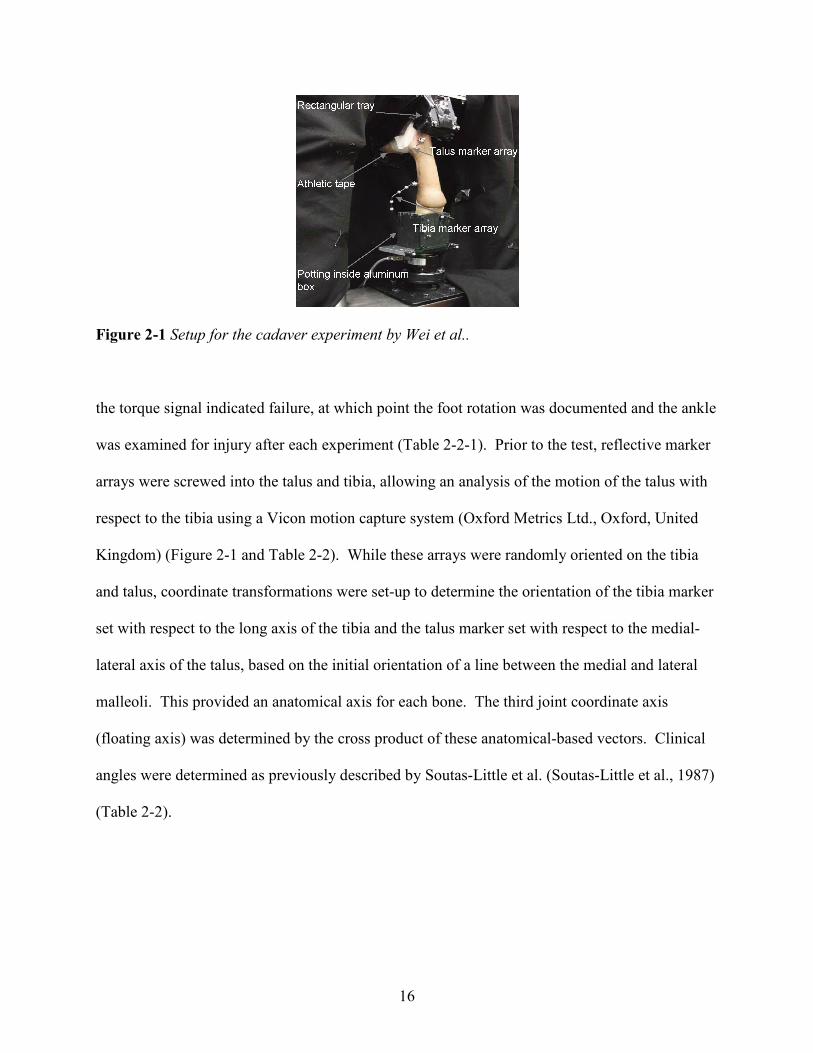
approximately 15 cm distal to the center of the knee (Wei et al., 2012b). The foot was taped to a

polycarbonate plate and inserted into a rectangular tray (Figure 2-1). Both the right and the left

limbs were dorsiflexed 20 degrees. The left limbs were positioned at 20 degrees of eversion,

while the right limbs were initially positioned in neutral with regard to the inversion/eversion

rotation prior to dynamic external foot rotation.

A compressive preload of 1500 N was applied axially and internal tibia rotation (external foot

rotation) was input in position control at a frequency of 1 Hz (0.5 seconds to peak rotation for

each test). The tests started with 20 degrees of rotation and then repeated in 10 degree

increments successively until an observed injury to the ankle. A steep drop in the magnitude of

16

Figure 2-1 Setup for the cadaver experiment by Wei et al..

the torque signal indicated failure, at which point the foot rotation was documented and the ankle

was examined for injury after each experiment (Table 2-2-1). Prior to the test, reflective marker

arrays were screwed into the talus and tibia, allowing an analysis of the motion of the talus with

respect to the tibia using a Vicon motion capture system (Oxford Metrics Ltd., Oxford, United

Kingdom) (Figure 2-1 and Table 2-2). While these arrays were randomly oriented on the tibia

and talus, coordinate transformations were set-up to determine the orientation of the tibia marker

set with respect to the long axis of the tibia and the talus marker set with respect to the medial-

lateral axis of the talus, based on the initial orientation of a line between the medial and lateral

malleoli. This provided an anatomical axis for each bone. The third joint coordinate axis

(floating axis) was determined by the cross product of these anatomical-based vectors. Clinical

angles were determined as previously described by Soutas-Little et al. (Soutas-Little et al., 1987)

(Table 2-2).

17

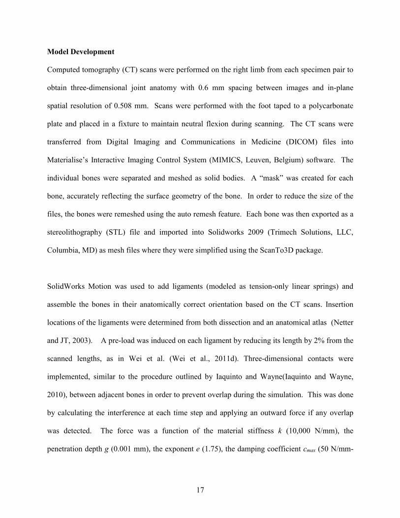
Model Development

Computed tomography (CT) scans were performed on the right limb from each specimen pair to

obtain three-dimensional joint anatomy with 0.6 mm spacing between images and in-plane

spatial resolution of 0.508 mm. Scans were performed with the foot taped to a polycarbonate

plate and placed in a fixture to maintain neutral flexion during scanning. The CT scans were

transferred from Digital Imaging and Communications in Medicine (DICOM) files into

Materialise’s Interactive Imaging Control System (MIMICS, Leuven, Belgium) software. The

individual bones were separated and meshed as solid bodies. A “mask” was created for each

bone, accurately reflecting the surface geometry of the bone. In order to reduce the size of the

files, the bones were remeshed using the auto remesh feature. Each bone was then exported as a

stereolithography (STL) file and imported into Solidworks 2009 (Trimech Solutions, LLC,

Columbia, MD) as mesh files where they were simplified using the ScanTo3D package.

SolidWorks Motion was used to add ligaments (modeled as tension-only linear springs) and

assemble the bones in their anatomically correct orientation based on the CT scans. Insertion

locations of the ligaments were determined from both dissection and an anatomical atlas (Netter

and JT, 2003). A pre-load was induced on each ligament by reducing its length by 2% from the

scanned lengths, as in Wei et al. (Wei et al., 2011d). Three-dimensional contacts were

implemented, similar to the procedure outlined by Iaquinto and Wayne(Iaquinto and Wayne,

2010), between adjacent bones in order to prevent overlap during the simulation. This was done

by calculating the interference at each time step and applying an outward force if any overlap

was detected. The force was a function of the material stiffness k (10,000 N/mm), the

penetration depth g (0.001 mm), the exponent e (1.75), the damping coefficient cmax (50 N/mm-

18

s), penetration depth at maximum damping dmax, and penetration velocitydt

dg. Friction and the

effects of gravity were considered negligible.

),( maxmax dcfdt

dgkgF e

n

+=

Since toe involvement was likely minimal in the cadaver study, the phalanges were excluded

from the model.

Figure 2-2 The cadaver taping pattern (a) and the model taping pattern represented by springs

(b). Note: for clarity all ligament springs and the plate springs on the medial side of the ankle

were set invisible.

c d e

a b

19

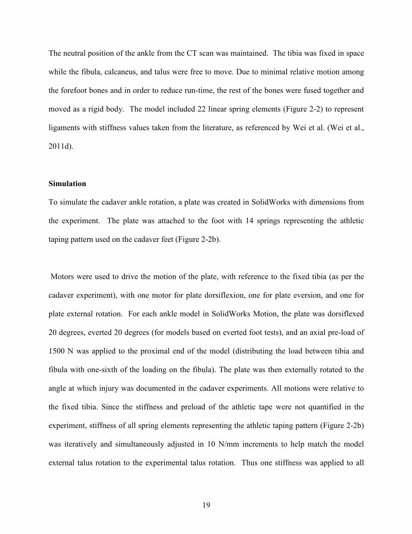
The neutral position of the ankle from the CT scan was maintained. The tibia was fixed in space

while the fibula, calcaneus, and talus were free to move. Due to minimal relative motion among

the forefoot bones and in order to reduce run-time, the rest of the bones were fused together and

moved as a rigid body. The model included 22 linear spring elements (Figure 2-2) to represent

ligaments with stiffness values taken from the literature, as referenced by Wei et al. (Wei et al.,

2011d).

Simulation

To simulate the cadaver ankle rotation, a plate was created in SolidWorks with dimensions from

the experiment. The plate was attached to the foot with 14 springs representing the athletic

taping pattern used on the cadaver feet (Figure 2-2b).

Motors were used to drive the motion of the plate, with reference to the fixed tibia (as per the

cadaver experiment), with one motor for plate dorsiflexion, one for plate eversion, and one for

plate external rotation. For each ankle model in SolidWorks Motion, the plate was dorsiflexed

20 degrees, everted 20 degrees (for models based on everted foot tests), and an axial pre-load of

1500 N was applied to the proximal end of the model (distributing the load between tibia and

fibula with one-sixth of the loading on the fibula). The plate was then externally rotated to the

angle at which injury was documented in the cadaver experiments. All motions were relative to

the fixed tibia. Since the stiffness and preload of the athletic tape were not quantified in the

experiment, stiffness of all spring elements representing the athletic taping pattern (Figure 2-2b)

was iteratively and simultaneously adjusted in 10 N/mm increments to help match the model

external talus rotation to the experimental talus rotation. Thus one stiffness was applied to all

20

those springs that represented the effect of tape. Ligament strains, defined in percentage as the

relative elongations of ligaments, were determined at the plate rotation needed to generate gross

ankle injury in the cadaver experiments (Table 2-1).

Two-sample t-tests were performed to compare failure strains for partial tears and total ruptures,

for comparing the model generated talus rotations with experimental talus rotations, for

comparing ATiFL failure strains with ADL failure strains, and for comparing experimental plate

rotations with experimental talus rotations. P values less than 0.05 were considered significant in

all tests.

RESULTS

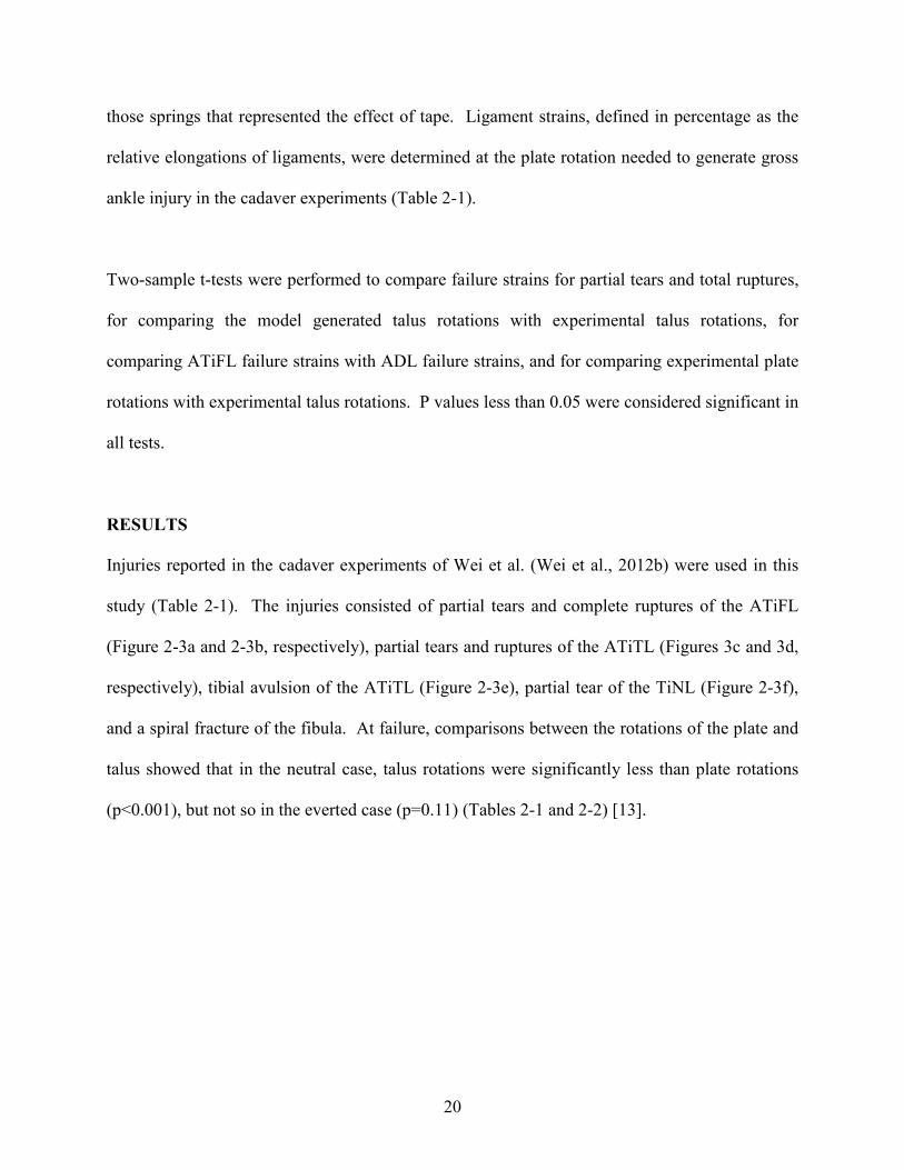
Injuries reported in the cadaver experiments of Wei et al. (Wei et al., 2012b) were used in this

study (Table 2-1). The injuries consisted of partial tears and complete ruptures of the ATiFL

(Figure 2-3a and 2-3b, respectively), partial tears and ruptures of the ATiTL (Figures 3c and 3d,

respectively), tibial avulsion of the ATiTL (Figure 2-3e), partial tear of the TiNL (Figure 2-3f),

and a spiral fracture of the fibula. At failure, comparisons between the rotations of the plate and

talus showed that in the neutral case, talus rotations were significantly less than plate rotations

(p<0.001), but not so in the everted case (p=0.11) (Tables 2-1 and 2-2) [13].

21

Figure 2-3 Injury mechanisms reported from the cadaver study by Wei et al. (Wei et al., 2012b).

Partial tear of the ATiFL (a); Rupture of the ATiFL (b); Partial tear of the ATiTL (c); Rupture

of the ATiTL (d); Tibial avulsion of the ATiTL (e); Partial tear of the TiNL(f). Note: the location

of injury is shown with a hemostat.

Lateral a b

Fibula

Tibia Medial

Anterior Posterior Tibia

Fibula

Lateral

Medial

Anterior Posterior

Tibia

Talus

Anterior Posterior Anterior Posterior

Tibia

Tibia

Medial

Lateral

Medial

Lateral

Posterior

Anterior

Tibia

Calcaneus

c d

e f

22

The stiffness of the simulated athletic tape was variable between specimens and between 300

N/mm to 400 N/mm. Comparisons of the talus rotations showed that the model generated talus

rotations were not statistically different than the experimental rotations (p>0.88) (Table 2-2).

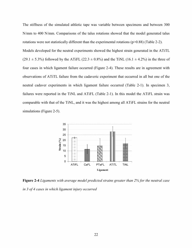
Models developed for the neutral experiments showed the highest strain generated in the ATiTL

(29.1 ± 5.3%) followed by the ATiFL (22.3 ± 0.8%) and the TiNL (16.1 ± 4.2%) in the three of

four cases in which ligament failure occurred (Figure 2-4). These results are in agreement with

observations of ATiTL failure from the cadaveric experiment that occurred in all but one of the

neutral cadaver experiments in which ligament failure occurred (Table 2-1). In specimen 3,

failures were reported in the TiNL and ATiFL (Table 2-1). In this model the ATiFL strain was

comparable with that of the TiNL, and it was the highest among all ATiFL strains for the neutral

simulations (Figure 2-5).

Figure 2-4 Ligaments with average model predicted strains greater than 2% for the neutral case

in 3 of 4 cases in which ligament injury occurred

23

Figure 2-5 Strains in the ATiFL and the two deltoid ligaments (ATiTL and TiNL) for the neutral

case for each specimen modeled

Computational models of the everted ankle experiments showed the highest strains in the ATiFL

(31.2 ± 4.3%) followed by the TiNL (18.5 ± 5.6%) and the ATiTL (18.1 ± 5.0%) (Figure 2-6).

These data coincided with the observation of ATiFL injury in all of these cadaver experiments

(Table 2-1). All but two of the specimens from the cadaver study suffered complete ruptures

(specimens 2 and 5 suffered partial tears) and the corresponding strains can be seen in Figure 2-

7. For ruptured ligament cases there was no significant difference between ATiFL failure strain

and ATiTL failure strain (p>0.7). For partial tears, there was no significant difference between

ATiFL failure strain and ADL failure strain (combining cases of ATiTL failure and TiNL

failure) (p>0.45).

24

Figure 2-6 Ligaments with average model predicted strains greater than 2% for the everted

simulations

Figure 2-7 Strains in the ATiFL and the two deltoid ligaments (ATiTL and TiNL) for the everted

simulations

25

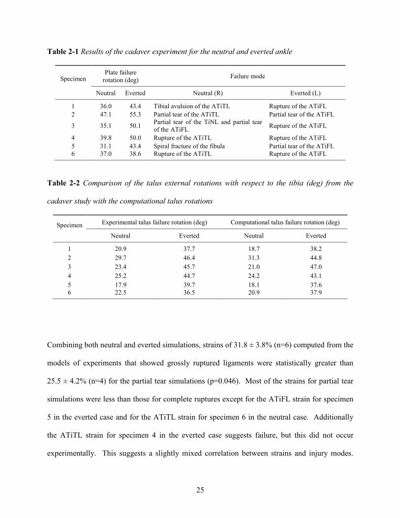
Table 2-1 Results of the cadaver experiment for the neutral and everted ankle

Specimen Plate failure

rotation (deg) Failure mode

Neutral Everted Neutral (R) Everted (L)

1 36.0 43.4 Tibial avulsion of the ATiTL Rupture of the ATiFL

2 47.1 55.3 Partial tear of the ATiTL Partial tear of the ATiFL

3 35.1 50.1 Partial tear of the TiNL and partial tear

of the ATiFL Rupture of the ATiFL

4 39.8 50.0 Rupture of the ATiTL Rupture of the ATiFL

5 31.1 43.4 Spiral fracture of the fibula Partial tear of the ATiFL

6 37.0 38.6 Rupture of the ATiTL Rupture of the ATiFL

Table 2-2 Comparison of the talus external rotations with respect to the tibia (deg) from the

cadaver study with the computational talus rotations

Specimen Experimental talus failure rotation (deg) Computational talus failure rotation (deg)

Neutral Everted Neutral Everted

1 20.9 37.7 18.7 38.2

2 29.7 46.4 31.3 44.8

3 23.4 45.7 21.0 47.0

4 25.2 44.7 24.2 43.1

5 17.9 39.7 18.1 37.6

6 22.5 36.5 20.9 37.9

Combining both neutral and everted simulations, strains of 31.8 ± 3.8% (n=6) computed from the

models of experiments that showed grossly ruptured ligaments were statistically greater than

25.5 ± 4.2% (n=4) for the partial tear simulations (p=0.046). Most of the strains for partial tear

simulations were less than those for complete ruptures except for the ATiFL strain for specimen

5 in the everted case and for the ATiTL strain for specimen 6 in the neutral case. Additionally

the ATiTL strain for specimen 4 in the everted case suggests failure, but this did not occur

experimentally. This suggests a slightly mixed correlation between strains and injury modes.

26

Furthermore, in the neutral model that suffered a spiral fracture experimentally (specimen 5), the

ATiFL, ATiTL and TiNL strains (23.6%, 10.4%, and 13.0%, respectively) were below failure

levels documented in other experiments. In the ATiTL avulsion case (specimen 1), the ATiFL

and TiNL strains (21.2% and 14.9%, respectively) were also below the average failure levels of

other simulations. The ATiTL strain, on the other hand, from the model was 32.2%, well above

the failure levels given in other simulations.

DISCUSSION

The study supported the hypothesis that the models would generate the highest strains in the

ATiFL for the everted foot and in the deltoid ligaments for the neutral foot. As suggested by

Wei et al. (Wei et al., 2012b), the lateral talar translation resulting from an everted foot puts

strain on the ATiFL by pushing the fibula away from the tibia, since the ligament is oriented

along the coronal plane. In the neutral foot, lateral talar translation was minimal during axial

load and external rotation, and thus external rotation resulted in straining the deltoid, as this

ligament is oriented along the sagittal plane. The study also confirmed that there was a

significant difference in strains for cases of complete versus partially ruptured ligaments. In the

neutral case, specimen 3 revealed the correct prediction of injury, despite yielding a different

result than the other simulations. In all other cases of a neutral foot ligament failure the ATiTL

experienced the highest strain, yet the highest strain in specimen 3 was found in the TiNL

followed by the ATiFL. This was consistent with the injuries generated in the TiNL and ATiFL

in the cadaver study (Table 2-1 and Figure 2-5). Furthermore, the rotations to failure for the

neutral foot in specimens 1, 3, and 6 were similar, yet corresponded to different computational

ligament strains (Figure 2-5) and this was supported by the observation of different injuries

(Table 2-1). This information indicates that specimen-specific modeling may, in some cases,

27

predict injuries that may not be predictable with a generic model, such as used previously by this

laboratory. While differences in the geometry of the trochlea tali and talar facets have both been

identified as potential explanations for differences between specimens, a detailed presentation of

these differences was beyond the scope of the current experiment.

While little data exists on the failure strains of the ankle ligaments of interest in this study, these

failure data are consistent with experimental failure calculations from other ligaments. A study

by Beumer et al. (Beumer et al., 2003), for example, reported the force required to rupture the

ATiFL, PTiFL, and posterior tibiotalar ligament (PTiTL) to be 500±105 N, 708 ±91 N, and

446±51 N, respectively. Using the stiffnesses from the literature (Wei et al., 2011d) and

ligament lengths from the simulations, the failure forces of the ATiFL, TiNL, respectively, were

610±98 N and 750±190 N, comparable to Beumer’s values, while the ATiTL prediction,

170±0N, was considerably lower. Attarian et al. (Attarian et al., 1985) measured failure strains

of bone-ligament-bone preparations in tensile experiments. They documented values of, on

average, 53% and 38% for the anterior talofibular ligament (ATaFL) and calcaneofibular

ligament (CaFL), respectively, which are higher than the failure strains reported in the current

study.

Given that ligament collagen fibers start to tear at approximately half of the failure strain (a so-

called grade I ligament sprain) (Yahia et al., 1990), the partial tears might be more representative

of grade II sprain injuries, as they occurred at approximately 70% of the total rupture strain.

Interestingly, the strains for non-injured ligaments fell below this partial-tear failure strain

average for all ligaments in the neutral simulation and all but one ligament (ATiTL for specimen

28

4) in the everted simulations. This may indicate a low risk of falsely predicting ligament failure

for non-injured ligaments in future injury simulation studies.

One limitation of the current study was that we were not able to accurately quantify the ankle-

tape structural stiffness of the cadaver study, and thus had to estimate it in our simulations. We

attempted to compensate for this aspect by adjusting the spring stiffness that represented the

taping of the foot to the plate for each specimen so that the motion of the model talus was similar

to that of the cadaver talus for a given level of plate rotation at failure. These values varied

between specimens, as the structural stiffness due to the amount of tape stretch in the cadaver

study may have actually varied between specimens. Despite potential errors in matching tape

stiffness, we believe that as long as the talar motions in the simulations closely matched those of

the experiments, the model’s ligament strains would provide reasonable estimates of strain.

Another limitation of the study was that it assumed simple, linear elastic behavior of the ankle

ligaments. While ligaments may behave linearly for small deformations, they do behave non-

linearly for failure strains. Because of this, non-linear computational models should be used for

failure-level studies in the future. The model also did not account for the viscoelastic properties

of ligaments. Funk et al. (Funk et al., 2000) produced non-linear models for eight major

ligaments of the foot-ankle complex, which accounted for both their elastic and viscoelastic

properties. They concluded that a viscoelastic assumption could also be neglected for very slow

(<0.0001/s) or very fast (>1/s) strain rates, but substantial effects seem to exist on ligament

behavior for intermediate strain rates. In the cadaver experiment by Wei et al. (Wei et al.,

2012b), the tibia rotation was input at 1 Hz, so the ligaments reached their maximum strain at

0.5s. This means that the failure strain rates were, on average, 1.000/s for partial tears and 0.933

29

/s for ruptures, indicating that there could be some viscoelastic effect. However, while the model

may not currently predict the exact mechanical behavior of ligaments, quantifying failure

ligament strains, rather than forces, may be a better indicator of injury tolerance due to the

viscoelastic nature of ankle ligaments (Edwards and Delee, 1984, Boytim et al., 1991). This may

be supported by earlier studies that show that the ultimate tensile strength of ligaments and

tendons increases significantly with strain rate, while ultimate strain does not (France et al.,

1987), (Ng et al., 2004). Yet, in order to improve upon the model in future predictions of ankle

ligament failure strains from in vitro and in vivo studies, more accurate constitutive modeling

would still seem to be warranted.

The use of specimen-specific ankle modeling could be expanded to investigate in vivo injury

cases simulating situations where the geometry and motion of the foot/ankle complex from a

specimen are known. For example, in the 2008 Beijing Olympic Games two ankle inversion

injuries were captured on film and analyzed using a model-based image matching (MBIM)

motion analysis technique from calibrated video sequences. The results of the study indicated a

disparity in injury mechanics from previous studies. Previous studies of lateral ankle injuries

suggest that the injurious motion involves inversion plus an internal rotation of the foot (Safran

et al., 1999) with plantarflexion (Vitale and Fallat, 1988). However, the MBIM study revealed

that plantarflexion was not involved in these ankle sprains, indicating that the talocrural joint was

less involved in these inversion ankle sprains (Mok et al., 2011). By combining the MBIM with

computational foot and ankle models developed from CT or magnetic resonance images (MRI),

ankle injury mechanisms may be better understood. Such studies could aid in the design of

intervention strategies and new equipment designs that might help limit the severity and

30

frequency of athletic ankle injuries. Based on the results of the current study, specimen-specific

modeling may help provide even better data for the study of ankle injury mechanics on the

athletic field.

31

CHAPTER 3:

EFFECT OF PRE-EVERSION ON TALOCRURAL AND SUBTALAR JOINT MOTION

DURING ANKLE EXTERNAL ROTATION

ABSTRACT

Eversion prior to excessive external foot rotation has been shown to predispose the anterior

tibiofibular ligament (ATiFL) to failure, yet protect the anterior deltoid ligament (ADL) from

failure despite high levels of foot rotation. The purpose of the current study was to measure the

rotations of both the subtalar and talocrural joints during foot external rotation in either a neutral

or a pre-everted position in order to better understand injury generated during rotation. Fourteen

(seven pairs) cadaver lower extremities were externally rotated 20 degrees in either a pre-everted

or neutral configuration. Marker arrays were screwed into the tibia, talus, and calcaneus and

motion capture was performed to track the motion of these bones. A joint coordinate system was

used to analyze motions of the two joints. While talocrural joint rotation was greater in the

neutral ankle (13.33 ± 2.09 deg versus 10.51 ± 2.75 deg, p=0.006), subtalar joint rotation was

greater in the pre-everted ankle (2.38 ± 1.89 deg versus 1.12 ± 1.04 deg, p=0.014). Overall, the

talocrural joint rotated more than the subtalar joint (11.92 ± 2.77 deg versus 1.75 ± 1.61 degrees,

p<0.001). It was proposed that the calcaneus and talus ‘lock’ in a neutral position, but ‘unlock’

when the ankle is everted prior to rotation. This locking/unlocking mechanism could be

responsible for an increased subtalar rotation, but decreased talocrural rotation when the ankle is

pre-everted, protecting the ADL from failure. This study may provide information valuable to

the study of external rotation kinematics and injury risk.

32

INTRODUCTION

Positioning of the ankle prior to external rotation affects the behavior of the talus and therefore

location of injury (Wei et al., 2012b, Button et al., 2013, Haraguchi and Armiger, 2009). A

previous study in this laboratory has shown that the combination of ankle eversion and

dorsiflexion followed by axial load and external rotation produces isolated anterior tibiofibular

ligament (ATiFL) injury, also known as high (or syndesmotic) ankle sprain. In a similar set of

experiments, removing the eversion component mostly results in anterior deltoid ligament (ADL)

injury, or a medial ankle sprain. Since the ATiFL restricts both fibular movement and external

talus rotation(Sarsam and Hughes, 1988), the mechanism of high ankle sprain is attributed to a

pre-tensioning of the ATiFL, as a result of the eversion and axial load, following by external

rotation of the talus(Wei et al., 2012b). Oriented approximately in the antero-posterior direction

in the sagittal plane (Wei et al., 2012b), the ADL is ruptured due to external rotation of the foot,

supported by a clinical review which states that external rotation of the foot will “first rupture the

deltoid ligament, with subsequent injury to the ATiFL” (Dattani et al., 2008, Wei et al., 2011d).

Yet, despite no observation of ADL injury in the pre-everted ankles, the amount of foot rotation

at failure was significantly higher than the failure rotation in neutral ankles (Wei et al., 2012b),

seemingly contradicting the notion that external foot rotation primarily strains the ADL.

However, while there is more overall foot rotation in the pre-everted ankles, ligament strain is

dependent on relative bone motion which was not documented at the point of failure in this

previous study.

While strain in the ADL is strongly correlated with talocrural joint rotation, it has been suggested

that the subtalar joint equally contributes to overall foot rotation (Siegler et al., 1988). Excessive

33

subtalar joint rotation could also be problematic due to increased risk of subtalar ligament injury,

which has been implicated in subtalar joint instability and calcaneal tilt (Kato, 1995, Heilman et

al., 1990). Previous studies have measured subtalar and talocrural joint rotation during

plantarflexion/dorsiflexion, inversion/eversion (Wong et al., 2005, Fassbind et al., 2011), and

passive rotation (Siegler et al., 1988). While these studies noted that the contribution of both the

subtalar and talocrural joints to foot rotation was dependent on the positioning of the ankle, they

did not document the effect of pre-eversion and axial load on joint motion during rotation. The

objectives of the current study were 1) to measure the contributions from the talocrural and

subtalar joints to the overall rotation of the foot-shank in an axially loaded foot and 2) to identify

the effect of pre-eversion on these contributions.

METHODS

Fourteen (seven pairs) fresh-frozen human cadaver (age 58.5 ± 9.2 years) lower-extremities were

used in this study. The limbs were stored at -20°C and thawed to room temperature for 24 hours

prior to testing. The tibia and fibula were transected 15 cm distal to the center of the knee, and

the proximal 10 cm of the bones was removed of tissue and cleaned with 70% alcohol. The

cleaned portion of the bone was potted in an aluminum box with room-temperature curing epoxy

(Fiber Strand, Martin Senior Corp., Cleveland, OH). Two screws were placed in the anterior and

medial tibia before potting to help restrain the tibia in the potting material. Reflective marker

arrays were screwed in the anterior medial aspect of the talus, posterior calcaneus, and on the

tibia approximately 20 cm proximal to the articular surface. CT scans verified the placement of

the marker arrays.

34

Figure 3-1 Cadaver foot taped to a polycarbonate plate (a). Ankle with reflective marker array

in the tibia, talus, and calcaneus in the testing fixture (b).

Elastic athletic tape (Elastikon, J&J, New Brunswick, NJ) was used to constrain the foot onto a

polycarbonate plate (32 cm x 8 cm) (Figure 3-1a). Experiments were performed with a

customized hydraulic biaxial testing machine with a 244 Nm rotary actuator (Model SS-001-1C,

b

a

35

Micromatic, Berne, IN) and a vertically oriented linear actuator (Model 204.52, MTS Corp.,

Eden Prairie, MN). The proximal (potted) end of the foot was attached to the rotary actuator

through a biaxial load cell (Model 1216CEW-2K, Interface, Scottsdale, AZ) with a capacity of

8896 N of axial force and 113 Nm of torsion (Figure 3-1b). Right ankles were pre-everted 20

degrees prior to rotation and left ankles were neutral in the coronal plane. A 1500 N

compressive preload was applied to simulate dynamic weight bearing prior to rotation and 20

degrees of internal tibia rotation (external foot rotation) was input in position control at 1Hz.

A Vicon motion capture system (Oxford Metrics Ltd, Oxford, UK) was used to document the

position of the marker arrays during motion. Coordinate transformations were performed on the

tibia, talus, and calcaneus marker arrays in order to establish orthogonal coordinate systems in

line with the three axes of the ankle (Figure 3-2). Joint coordinate systems (JCS) were

established between the tibia and talus (talocrural joint) and between the talus and calcaneus

(subtalar joint), similar to previously defined systems (Soutas-Little et al., 1987, Wu et al.,

2002). Calculations for flexion, rotation, and inversion/eversion of the talocrural joint are shown

below (Equations 1-2) (note: the same procedure is used for the subtalar joint).

�� = �� [1a]

�� = �� [1b]

� =�� ×��

|�� ×��| [1c]

� = �� ∙ �� (flexion) [2a]

� = �� ∙ �� (rotation) [2b]

� = �� ∙ �� (inversion/eversion) [2c]

36

Figure 3-2 Orthogonal coordinate axes on the tibia, talus, and calcaneus.

Paired t-tests were used to compare the amount of joint flexion, rotation, and inversion/eversion

between neutral and everted ankles. Two-way repeated measures ANOVA (pre-positioning,

joint) was used to compare the amount of flexion, rotation, and inversion/eversion between the

two joints. P-values less than 0.05 were considered significant in all tests.

RESULTS

Motions of the subtalar and talocrural joints during 20 degrees of internal tibia rotation were

shown in Table 3-1 (Note: talocrural motion refers to talus motion with respect to the tibia, while

subtalar motion refers to calcaneus motion with respect to the talus). There was significantly

more external rotation in the talocrural joint compared with the subtalar joint (p<0.001).

Additionally there was significantly more talocrural external rotation (p=0.006), but significantly

37

less subtalar external rotation (p=0.014) in the neutral foot when compared with the pre-everted

foot.

Table 3-1 Motions of the subtalar and talocrural joint for 20 degrees of external rotation

DISCUSSION

While previous studies have investigated the effects of ankle pre-eversion on location of injury

and strain generated in key ankle ligaments during external rotation of an axially-loaded foot

(Button et al., 2013, Wei et al., 2012b), the current study examined the effects that pre-eversion

had on talocrural and subtalar joint movement. Specifically, a key aim of the current study was

to investigate why pre-everted ankles saw no ADL injury despite high levels of foot rotation at

failure. The study involved using a JCS to calculate joint motion during 20 degrees of external

ankle rotation in either a pre-everted or a neutral foot. Results of the study indicated that when

the foot was axially loaded and externally rotated most of the foot-shank rotation comes from the

talocrural joint. However, pre-eversion lowered the amount of talocrural rotation, potentially

lowering ADL injury risk.

Neutral Everted Neutral Everted Neutral Everted Neutral Everted Neutral Everted Neutral Everted

0.59 0.29 0.39 0.19 1.46 0.16 0.03 0.34 0.04 0.69 15.81 11.08

1.66 2.43 2.68 3.80 2.24 1.43 0.98 4.09 1.11 1.70 12.30 10.97

0.50 0.21 1.53 1.03 1.29 0.75 3.11 3.50 2.53 5.78 11.84 6.41

0.25 0.32 1.35 0.30 0.97 0.53 0.55 0.52 0.23 0.88 15.67 12.87

0.97 0.41 1.30 1.34 0.84 0.16 0.79 0.02 0.02 0.94 14.93 14.20

1.04 1.99 1.50 1.31 1.23 1.02 2.91 0.78 1.98 2.88 12.09 10.53

1.71 0.84 0.58 0.85 0.04 0.52 0.72 0.48 1.90 3.81 10.65 7.52

0.96 0.93 1.33 1.26 1.15 0.65 1.30 1.39 1.12 2.38 13.33 10.51

0.56 0.91 0.74 1.21 0.67 0.46 1.21 1.67 1.04 1.89 2.09 2.75

Talocrural

Dorsiflexion

(deg)

Subtalar

Rotation (deg)

Talocrural

Rotation (deg)

1

2

3

4

5

Specimen

Subtalar

Eversion (deg)

Talocrural

Eversion (deg)

Subtalar

Dorsiflexion

(deg)

6

7

AVG

STDEV

p-value0.39 0.79 0.054 0.882 0.014 0.006

0.787 0.197 <0.001

38

The geometry of the subtalar joint may explain the differences in rotation between the subtalar

and talocrural joints. The talus contacts the calcaneus on two articular surfaces: the subtalar

posterior joint and anterior subtalar joint (Viladot et al., 1984). The calcaneal surface on the

medial section of the anterior subtalar joint is called the “sustenaculum tali”, which the

articulating surface of the talus fits into (Figure 3-3) (Viladot et al., 1984), and the movement of

this complex is fundamental to the transmission of rotations from the foot to leg (Leardini et al.,

2001). In a neutral ankle, the sustentaculum tali may ‘lock’ with the articulating surface of the

talus, restricting its rotation (Figure 3a,b). As a result, when the tibia rotates, this ‘locking’

restricts the talus from rotating with the tibia, resulting in a high talocrural rotation between the

tibia and talus. In contrast, when the ankle is everted, (Figure 3-3c,3-d) the contact between the

sustentaculum tali and articulating surface of the talus ‘unlocks’. Consequently, this ‘unlocking’

enables the tibiotalar ligaments to pull the talus with the rotation of the tibia, resulting in lower

relative motion.

This phenomenon can possibly explain the injuries observed in the Wei et al. study (Wei et al.,

2012b). In that study, the neutral ankles experienced ADL injury in 5 of 6 cases while the pre-

everted ankles experienced no instances of ADL injury, despite failing at significantly higher

foot rotations. Since the ADL is the primary ligament resisting ankle rotation (Wei et al.,

2011d), one would have expected the significantly higher foot rotation in the everted ankles to

fail the ADL as well. However, results of the current study may imply that even though the pre-

everted ankles experienced more foot rotation at failure in Wei et al. (2012), the ‘unlocking’ of

the subtalar joint (due to pre-eversion) might have protected the ADL from failure by limiting

talocrural joint rotation. As suggested by Wei et al. (2012), axial loading may have translated

39

the talus laterally, thereby pushing the fibula away from the tibia, producing pre-strain in the

ATiFL, and potentially predisposing the foot to a high ankle sprain. Increased subtalar joint

rotation in the pre-everted ankles of the current study potentially could increase the risk of

subtalar ligament failure, resulting in chronic instability of the joint. On the other hand, the

subtalar joint remained ‘locked’ in the neutral scenario, explaining ADL injury for these ankle

(Wei et al., 2012b).

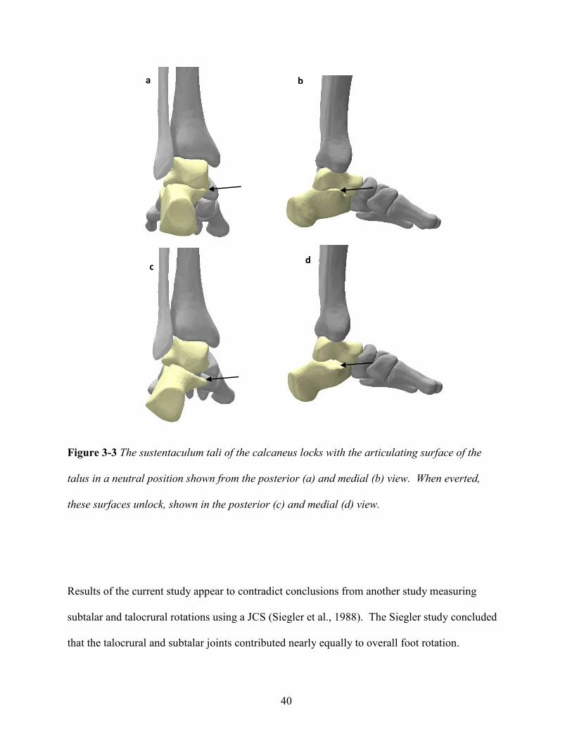
40

Figure 3-3 The sustentaculum tali of the calcaneus locks with the articulating surface of the

talus in a neutral position shown from the posterior (a) and medial (b) view. When everted,

these surfaces unlock, shown in the posterior (c) and medial (d) view.

Results of the current study appear to contradict conclusions from another study measuring

subtalar and talocrural rotations using a JCS (Siegler et al., 1988). The Siegler study concluded

that the talocrural and subtalar joints contributed nearly equally to overall foot rotation.

a b

c d

41

However, that study involved applying rotation to an unloaded ankle, while the current study

involved preloading the joint with 1500 N. The difference in experimental results of the two

studies may suggest that compressing the subtalar joint prior to rotation may be essential for the

‘locking’ mechanism to occur—suggesting that axial load may increase the risk of ADL injury.

A limitation of the current study was that the tests were run at sub-failure levels. While the

motions of the joints at failure levels could be estimated based on extrapolations of the motions

from this study, a future failure-level study is warranted. Additionally, the Wei 2012 failure-

level study involved pre-dorsiflexion to both neutral and everted ankles (Wei et al., 2012b),

while the current study did not. While pre-dorsiflexing the ankles in the current study may have

better replicated the previous experiment, a previous parametric study concluded that pre-

dorsiflexion has little effect on ADL strain during external rotation (Wei et al., 2011b) indicating

that pre-dorsiflexion may have changed the results of this study very little.

In conclusion, everting the foot prior to external rotation affects the kinematics of the subtalar

and talocrural joints. When the ankle is in neutral, the subtalar joint ‘locks’, restricting rotation

of the joint and straining the ADL. Everting the ankle prior to rotation ‘unlocks’ the subtalar

joint which allows the talus to rotate with the tibia, potentially limiting ADL strain and putting

the primary strain on the ATiFL. This study may improve our understanding of the various

mechanisms of ankle injury during external rotation of the foot.

42

CHAPTER 4:

ROTATIONAL STIFFNESS OF AMERICAN FOOTBALL SHOES AFFECTS ANKLE

BIOMECHANICS AND INJURY SEVERITY

ABSTRACT

While previous studies have investigated the effect of shoe-surface interaction on injury risk, few

studies have examined the effect of shoe rotational stiffness. The hypothesis of the current

study was that ankles externally rotated to failure in shoes with low rotational stiffness would

allow more talus eversion than those in shoes with a higher rotational stiffness, resulting in less

severe injury. Twelve (six pairs) cadaver lower extremities were externally rotated to gross

failure while positioned in 20 degrees of pre-eversion and 20 degrees of pre-dorsiflexion by

fixing the distal end of the foot, axially loading the proximal tibia, and internally rotating the

tibia. One ankle in each pair was constrained by an American football shoe with a stiff upper,

while the other was constrained by an American football shoe with a flexible upper.

Experimental bone motions were input into specimen-specific computational models to measure

ligament strains at failure. Ankles in flexible shoes failed at 97.4 ± 47.0 Nm which was greater

than the failure torque for ankles in stiff shoes (89.2 ± 44.9 Nm, p=0.049) in addition to allowing

6.7 ± 2.4 degrees of talus eversion during rotation, significantly greater than the 1.7 ± 1.0

degrees for ankles in stiff shoes (p=0.01). The significantly greater eversion in flexible shoes

was potentially due to a more natural response of the ankle during rotation, possibly affecting the

injuries that were produced. All ankles failed by either medial ankle injury or syndesmotic

injury, or a combination of both. Complex (more than one ligament or bone) injuries were noted

in 4 of 6 ankles in stiff shoes and 1 of 6 ankles in flexible shoes. Models of ankles in flexible

shoes showed significantly less strain in the deltoid at failure (p=0.023), but significantly more

43

strain in three of four subtalar ligaments (p=0.025, 0.03, and 0.047). The current study suggests

flexibility (or rotational stiffness) of the shoe may play an important role in both the risk and

severity of ankle injuries for athletes.

INTRODUCTION

Ankle injury can result from a variety of loading situations and accounts for 10-30% of all sports

injuries (Waterman et al., 2011). In American football, ankle injuries can occur in contact and

noncontact situations, but frequently the mechanism of injury involves a foot planted on the

playing surface with internal rotation of the upper body (Williams et al., 2007). This external

rotation of the foot with respect to the body is known to result in both medial and syndesmotic

ankle injuries (Waterman et al., 2011), as well as acute bone fractures (Haraguchi and Armiger,

2009, Laugehansen, 1950), and makes up 10-15% of all ankle injuries (Gerber et al., 1998, Fallat

et al., 1998). While less common than other types of ankle injuries, syndesmotic and medial

ankle injuries are of particular interest to researchers due to their long recovery time (Boytim et

al., 1991), and the potential for chronic ankle dysfunction (Gerber et al., 1998, Waterman et al.,

2011, Wolfe et al., 2001).

Syndesmotic ankles sprains (also known as high ankle sprains) involve injury to the anterior

tibiofibular ligament (ATiFL). While most clinical literature attribute high ankle sprains to

external rotation (Norkus and Floyd, 2001), a recent study with cadavers has produced high

ankle sprain when the ankles are everted (rotated about the long axis of the foot (Figure 4-1))

prior to external rotation (Wei et al., 2012b). The same study indicates that when keeping the

ankle neutral in the coronal plane (no eversion), external rotation results in medial ankle injury,

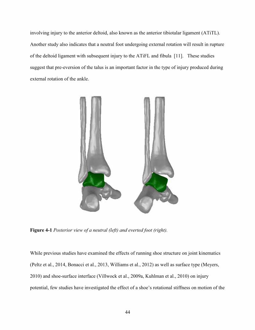
44

involving injury to the anterior deltoid, also known as the anterior tibiotalar ligament (ATiTL).

Another study also indicates that a neutral foot undergoing external rotation will result in rupture

of the deltoid ligament with subsequent injury to the ATiFL and fibula [11]. These studies

suggest that pre-eversion of the talus is an important factor in the type of injury produced during

external rotation of the ankle.

Figure 4-1 Posterior view of a neutral (left) and everted foot (right).

While previous studies have examined the effects of running shoe structure on joint kinematics

(Peltz et al., 2014, Bonacci et al., 2013, Williams et al., 2012) as well as surface type (Meyers,

2010) and shoe-surface interface (Villwock et al., 2009a, Kuhlman et al., 2010) on injury

potential, few studies have investigated the effect of a shoe’s rotational stiffness on motion of the

45

talus and the subsequent type and risk of ankle injury. One recent study, however, investigated

the role of an American football shoe’s rotational stiffness on talus motion at sub-injurious levels

(Wei et al., 2012a). The study involved rotating cadaver ankles in either stiff or flexible shoes,

while tracking motion of the talus with respect to the tibia. The results show that ankles in

flexible shoes experience more eversion of the talus with respect to the tibia, but less external

rotation. In addition to this sub-failure study, another cadaver study (Haraguchi and Armiger,

2009), using a rigid foot constraint, shows that external rotation of the ankle results in deltoid

injury prior to ATiFL injury with fibular fracture. Other studies (Wei et al., 2011d) suggest that

more subtalar motion and arch collapse occur with a more flexible constraint of the ankle, thus

allowing a more ‘natural’ response of the foot during external rotation of the ankle. As

suggested by Lundberg et al., these ‘natural’ motions of the ankle bones may act as a torsion

dissipating devices to increase the ankle’s resistance to injury (Lundberg et al., 1989a).

Computational models of the ankle have previously been utilized to understand how different

boundary conditions affect the biomechanics and ligament strains in the ankle under external

rotation (Button et al., 2013, Wei et al., 2011d). Given the complicated manner in which the

various ankle structures develop strain in the three planes of motion (Lin et al., 2006), these

models have the advantage of quickly determining ligament strains and reaction forces during

solid-body motion of the ankle. By inputting motions from experimental studies, the simulations

can provide information about the foot’s ability to respond to a given motion with various

constraints. The current plan was to develop a model to help in the assessment of different

footwear during injurious scenarios.

46

The purpose of the current study was to utilize a setup similar to a previous study (Wei et al.,

2012a), but rotate the ankles to failure in order to investigate the effect of shoe stiffness on injury

risk and type of injury. In order to produce conditions that result in high ankle sprain, the ankles

were pre-dorsiflexed and pre-everted, per a previous study (Wei et al., 2012b). Additionally, the

bone motions were input into specimen-specific computational models in order to study ankle

ligament strains and compare these to experimental injuries. The hypothesis of the study was

that ankles in flexible shoes would allow more talus eversion during external rotation of the foot

than those in stiff shoes, thus allowing the subtalar ligaments to carry some of the applied torque

and result in a less severe ankle injury.

METHODS

Shoe Selection

Shoes were selected based on a previous experimental study (Wei et al., 2012a). Briefly, four

styles of American football shoes were tested in order to determine rotational stiffness using a

surrogate (rigid) ankle. The four shoes were subjected to a compressive pre-load of 1500 N, a

rotational pre-torque of 2 Nm, and a dynamic torque of 60 Nm input in load control at a

frequency of 1 Hz. The rotational stiffness of the shoes was defined as the slope of the loading

portion of the torque-rotation curve. The study found that the shoe with the highest rotational

stiffness (50.0 ± 1.7 Nm/deg) was the Nike Flyposite and the lowest rotational stiffness (21.9 ±

2.8 Nm/deg) was the Nike Air (Wei et al., 2012a) (Figure 4-2). These two styles of shoe were

selected for the current study.

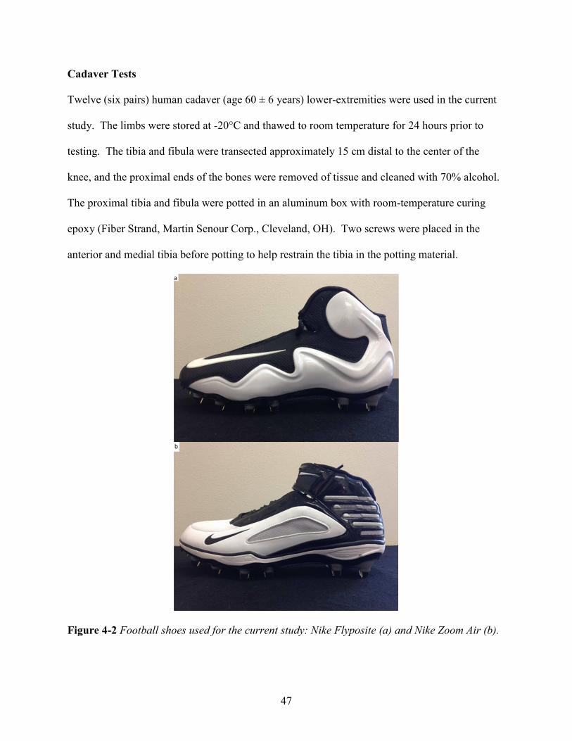
47

Cadaver Tests

Twelve (six pairs) human cadaver (age 60 ± 6 years) lower-extremities were used in the current

study. The limbs were stored at -20°C and thawed to room temperature for 24 hours prior to

testing. The tibia and fibula were transected approximately 15 cm distal to the center of the

knee, and the proximal ends of the bones were removed of tissue and cleaned with 70% alcohol.

The proximal tibia and fibula were potted in an aluminum box with room-temperature curing

epoxy (Fiber Strand, Martin Senour Corp., Cleveland, OH). Two screws were placed in the

anterior and medial tibia before potting to help restrain the tibia in the potting material.

Figure 4-2 Football shoes used for the current study: Nike Flyposite (a) and Nike Zoom Air (b).

48

For each pair of lower extremities, one foot was randomly fit into the stiff shoe and the other

foot was fit into a flexible shoe and equal numbers of right and left feet were assigned to the

different shoe types. Shoes were selected to fit the size of each cadaver ankle. Regular-length

cotton socks were used on each ankle. The base of the shoe was held by an epoxy cleat mold

(Figure 4-3), which was attached to the testing fixture (Figure 4-4). Each shoe, with an attached

mold in an aluminum tray, was dorsiflexed 20 degrees and everted 20 degrees to replicate

conditions that previously produced high ankle sprains during external rotation of the foot (Wei

et al., 2012b).

Figure 4-3 Football cleat mold made of epoxy resin used to fix the shoe to the testing fixture

Experiments were performed with a customized hydraulic biaxial testing machine with a 244 Nm

rotary actuator (Model SS-001-1C, Micromatic, Berne, IN) and a vertically oriented linear

actuator (Model 204.52, MTS Corp., Eden Prairie, MN). The proximal (potted) end of the foot

49

was attached to the rotary actuator through a biaxial load cell (Model 1216CEW-2K, Interface,

Scottsdale, AZ) with a capacity of 8896 N of axial force and 113 Nm of torsion (Note: because

of the high resistive torque for specimen 6, another load cell (Model 6467-107, serial #229,

Lowell) with a capacity of 20kN of axial force and 1130 Nm of torsion was used). The distal

end of the extremity was then attached to the aluminum tray via the cleat mold. The tray was

attached to a plate that allowed for x-y adjustments to align the tibia with the linear and torsional

actuators. A 1500 N compressive preload was applied to simulate dynamic weight bearing prior

to rotation, as used in previous studies (Wei et al., 2012b). Internal tibia rotation (external foot

rotation) was input in position control at 1 Hz (0.5s to peak rotation). The first experiment was

to 20° rotation and subsequent experiments were repeated on the same ankle in increments of 10°

until the torque signal indicated an injury (Figure 4-5). At failure, tibia rotation and torque were

documented. Dissections of the ankle (by MCS) were performed after joint failure.

50

Figure 4-4 The experiments were performed on a biaxial testing machine with the motions of the

talus and tibia tracked by a 5-camera motion capture system.

Figure 4-5 An example of the torque data from a sub-failure (a) and a failure (b) test. The

failure occurs when there is a steep drop in torque, as indicated by the arrow.

51

Motion Analysis

Reflective marker arrays were screwed into the anteriomedial aspect of the talus and on the tibia

approximately 20 cm proximal to the articular surface. Care was taken not to damage any

ligaments during marker insertion. CT scans verified the placement of the marker arrays. A

Vicon motion capture system (Oxford Metrics Ltd, Oxford, UK) was used to document the

position of the markers during the experiments. A joint coordinate system (JCS), as defined by

the International Society of Biomechanics (ISB) (Wu et al., 2002), was established between the

talus and tibia to determine the talocrural motions (talus motion with respect to the tibia) up to

ankle failure. This involved aligning the local coordinate systems (based on the reflective

marker triad) on the talus and tibia (Figure 4-4) with their respective anatomical axes through

coordinate transformations. The JCS took one coordinate axis from each of these local

coordinate systems and a final floating coordinate axis perpendicular to the other two. By

calculating the dot product between the coordinate axes, as described by the ISB, the amount of

ankle flexion, eversion, and rotation was determined at joint failure.

Figure 4-6 Lateral (a), posterior (b), and medial (c) views of one of the specimen-specific

models in SolidWorks with linear springs representing ligaments.

52


Model development has been previously described in depth (Button et al., 2013). Briefly,

specimen-specific computational models were created based on CT scans (0.6 mm per slice) of

each ankle specimen. Digital Imaging and Communications in Medicine (DICOM) files of each

specimen were imported into Materialise’s Interactive Medical Imaging Control System

(MIMICS)(Materialise, Ann Arbor, MI), yielding three-dimensional surface models of the bones

as Stereolithography (STL) files. Motion data from the JCS analysis were used to drive each

specimen-specific computational model. Nineteen linear springs were used to model ankle

ligaments and nine linear springs were used to model the tibiofibular interosseous ligament

(Figure 4-6); with the initial length reduced 2% prior to motion in order to induce a small pre-

load in each ligament to represent in situ pre-tensions (Liacouras and Waynel, 2007). Ligament

stiffness values were taken from the literature, as described by Wei et al. (Wei et al., 2011d).

Three-dimensional contacts were implemented between adjacent bones in order to prevent

overlap during simulation, with the parameters for the contact described previously by Button et

al. (Button et al., 2013). The forefoot was fixed and motors simulating rotation of the tibia and

talus, eversion of the talus, and the bone displacement as a result of axial pre-load were used to

drive each model. The calcaneus was fixed in the inferior-superior direction simulating contact

between the hind foot and the shoe. Strains were documented at the experimental point of gross

ankle failure.

Statistical Analysis

Paired t-tests were used to compare the differences between shoe constraints in failure torque,

talocrural eversion at failure, talocrural eversion per degree tibia rotation, talocrural rotation at

53

failure, talocrural rotation per degree of tibia rotation, and ligament strain. A one-way chi-square

test was used to test for a difference in complex injury rates in the two different shoe types. A

multiple regression analysis with categorical factors (subject, shoe) was used to analyze the

correlation between torque and eversion. P-values less than 0.05 were considered significant.

RESULTS

Experimental

Table 4-1 summarizes the injury mechanisms and failure metrics. The ankles in flexible shoes

failed at an average torque of 97.4 ± 47.0 Nm, significantly higher than the failure torque in stiff

shoes, 89.2 ± 44.9 Nm (p=0.049). While there was no difference in tibia failure rotation

(p=0.53) or talocrural failure rotation (p=0.51) between flexible and stiff shoes, there was

significantly more talocrural eversion at failure for ankles in flexible shoes (6.7 ± 2.4 versus 1.7

± 1.0, p=0.01).

54

Table 4-1 Summary of the injury mechanisms and failure metrics (* indicates significant difference between stiff and flexible shoes)

Stiff Flexible Stiff Flexible Stiff Flexible Stiff Flexible

1 85.6 83.4 44.7 46.5 19.3 17.5 3.5 3.9

5 102.4 117.9 37.4 43.0 13.9 15.1 2.0 8.2

Average 89.2 97.4 40.2 42.7 21.5 19.0 1.7 6.7*

Standard

Deviation44.9 47.0 6.9 11.6 5.6 4.9 1.0 2.4

5.20.818.5

Injury Mechanism

ATiFL rupture

Talocrural

Failure Eversion

(deg)

0.9 7.475.8

Stiff Flexible

Specimen

Talocrural

Failure Rotation

(deg)

Tibia Failure

Rotation (deg)

Failure Torque

(Nm)

2) ATiTL avulsion

1) ATiFL rupture

2 )ATiTL rupture

1) Medial malleolus fracture

2) Spiral fracture of the fibulaATiFL avulsion

ATiFL avulsion Fibular head fracture

ATiTL rupture1) ATiFL rupture

2) ATiTL rupture

Medial malleolus fracture1) ATiFL avulsion

61) ATiFL rupture

2) ATiTL ruptureATiTL rupture10.41.127.220.363.2

13.9

28.4

19.3

31.1

33.2 5.11.729.459.055.8

39.4 27.9 21.537.093.4

48.1

44.651.044.9

2

3

4

179.7170.7

55

Table 4-2 Strains at failure rotation for the anterior tibiofibular ligament (ATiFL), anterior tibiotalar ligament (ATiTL), posterior

tibiotalar ligament (PTiTL), interosseous talocalcaneal ligament (ITaCL), lateral talocalcaneal ligament (LTaCL), medial

talocalcaneal ligament (MTaCL), and posterior talocalcaneal ligament (PTaCL). (Underlining represents ligaments that ruptured or

avulsed)

Stiff Flexible Stiff Flexible Stiff Flexible Stiff Flexible Stiff Flexible Stiff Flexible Stiff Flexible

1 19.9 21.2 18.9 14.6 14.9 17.2 11.4 14.3 16.0 16.7 0.1 2.9 9.1 12.0

2 35.5 34.4 37.2 28.3 1.8 10.6 3.0 18.8 1.8 18.1 1.9 2.0 1.9 17.4

3 19.1 21.1 34.6 20.7 10.3 12.3 3.8 1.3 1.9 11.1 11.9 1.7 1.9 1.8

4 18.3 7.3 26.8 20.0 5.5 8.0 1.9 11.7 1.9 1.4 2.0 17.3 7.2 18.1

5 33.4 32.8 4.2 2.0 17.4 19.8 3.7 10.8 20.0 31.1 2.7 1.8 18.3 22.8

6 29.8 15.9 32.9 31.6 7.7 23.3 1.9 7.5 2.0 15.3 20.9 30.7 9.0 12.5

Average 26.0 22.1 25.7 19.5 9.6 15.2 3.3 10.7 7.3 15.6 6.6 9.4 7.9 14.1

Standard

Deviation8.5 10.9 13.3 9.8 6.4 4.8 4.4 6.4 8.9 10.8 4.7 16.2 6.8 8.0

LTaCL MTaCL PTaCL

Percent Elgonation at Failure Rotation (%)

Specimen

ATiFL ATiTL PTiTL ITaCL

56

Additionally, the amount of talocrural eversion per degree tibia rotation in the flexible shoe (0.16

± 0.04 degree/degree) was significantly greater than that for the stiff shoe (0.04 ± 0.02

degree/degree (p=0.023)). There was slightly more talocrural rotation per degree of tibia rotation

in the stiff shoe versus the flexible shoe (0.55 ± 0.16 degree/degree and 0.45 ± 0.10

degree/degree, respectively), although this was not quite significant (p=0.082). There was no

correlation between torque and eversion at failure (p=0.189).

The injury mechanisms also differed between the two types of shoes (Figure 4-7 and Table 4-1).

Medial injuries were observed in 5 of 6 stiff-shoe ankles and 3 of 6 flexible-shoe ankles.

Syndesmotic injuries were observed in 5 of 6 stiff-shoe ankles and 4 of 6 flexible-shoe ankles.

When the specimens were compared with a chi-square analysis, the effect of shoe type on the

frequency of complex injuries was not quite significant (p=0.079): there were combination

(complex) medial and syndesmotic injuries in 4 of 6 stiff-shoe ankles while only 1 of 6 ankles in

the flexible shoes suffered combination injuries. Bone injuries were also more prevalent in stiff-

shoe ankles, occurring three times compared with only one occurrence in flexible-shoe ankles.


Results of the SolidWorks simulations are shown in Table 4-2 for the seven ligaments that

developed the highest levels of strain during external rotation of the ankle: the ATiFL, ATiTL,

posterior tibiotalar ligament (PTiTL), interosseous talocalcaneal ligament (ITaCL), lateral

talocalcaneal ligament (LTaCL), medial talocalcaneal ligament (MTaCL), and posterior

talocalcaneal ligament (PTaCL). Models of the stiff and flexible shoe cases showed no

difference in ligament strains for the ATiFL (p=0.221) and MTaCL (p=0.264) at ankle failure.

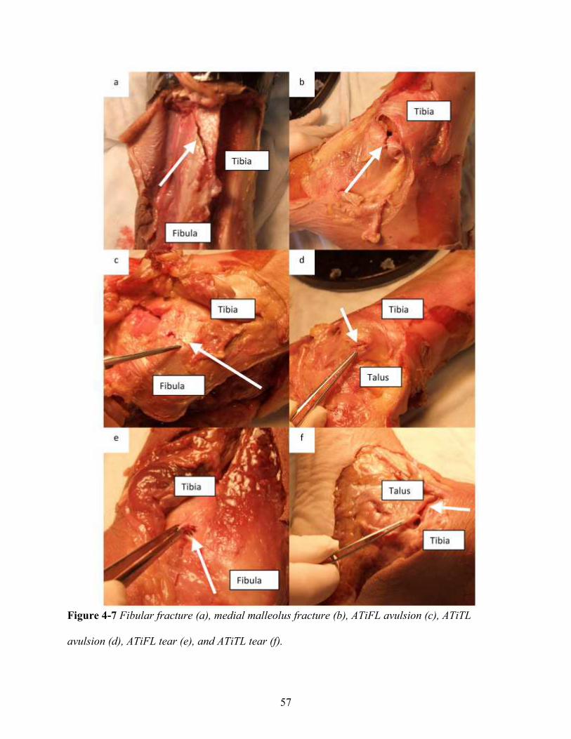
57

Figure 4-7 Fibular fracture (a), medial malleolus fracture (b), ATiFL avulsion (c), ATiTL

avulsion (d), ATiFL tear (e), and ATiTL tear (f).

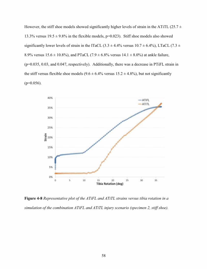
58

However, the stiff shoe models showed significantly higher levels of strain in the ATiTL (25.7 ±

13.3% versus 19.5 ± 9.8% in the flexible models, p=0.023). Stiff shoe models also showed

significantly lower levels of strain in the ITaCL (3.3 ± 4.4% versus 10.7 ± 6.4%), LTaCL (7.3 ±

8.9% versus 15.6 ± 10.8%), and PTaCL (7.9 ± 6.8% versus 14.1 ± 8.0%) at ankle failure,

(p=0.035, 0.03, and 0.047, respectively). Additionally, there was a decrease in PTiFL strain in

the stiff versus flexible shoe models (9.6 ± 6.4% versus 15.2 ± 4.8%), but not significantly

(p=0.056).

Figure 4-8 Representative plot of the ATiFL and ATiTL strains versus tibia rotation in a

simulation of the combination ATiFL and ATiTL injury scenario (specimen 2, stiff shoe).

59

In all four cases of complex ligamentous injury, the combination of pre-dorsiflexion, pre-

eversion, and axial load pre-strained the ATiFL more than the ATiTL. This resulted in higher

ATiFL strains for low levels of rotation, but an increasing ATiTL strain at near-failure levels of

rotation, while the ATiFL strain leveled off. In models 2, 4, and 6, the ATiTL strain level

surpassed the ATiFL strain in the last 3-5° of rotation before failure. In the other case

(specimen 3 flexible) the ATiTL strain nearly equaled the ATiFL strain, but did not surpass it. A

representative plot of simulations that showed combined ATiFL/ATiTL failure is shown in

Figure 4-8 (specimen 2, stiff shoe).

DISCUSSION

The rotational stiffness of American football shoes may affect high and medial ankle injury risks.

The current study investigated this premise by rotating pairs of cadaver ankles to failure in either

a stiff or flexible shoe. All ankles showed high or medial ankle injury, or a combination of each.

The ankles in flexible shoes failed at statistically higher torques and at significantly higher levels

of talocrural eversion than the ankles in stiff shoes. Computational models simulating flexible

shoe experiments exhibited statistically higher strains in subtalar ligaments during experimental

rotations, but lower strains in the ATiTL. Additionally, there was a higher frequency of complex

(combination) injuries in the stiff shoes, but not quite at a significant level. These results

indicate that shoes with a flexible upper may result in less severe ankle injuries than those with a

stiff upper.

60

The increased ankle eversion in the flexible shoe may be due to less restriction of the subtalar

joint to allow more motion between the talus and calcaneus, which may more closely simulate

the ankle’s natural, unrestrained response to external rotation. Previous investigations on

anatomical specimens have concluded that external rotation of the unrestrained ankle results in

pronation (the combination of eversion, abduction, and dorsiflexion) of the ankle (Lundberg et

al., 1989b). Rotations about the anteroposterior and vertical axes of the talonavicular joint have

been shown larger than the external rotation input about the tibia (Vanlangelaan, 1983). This is

described as the natural ‘transferal of rotation’ (Lundberg et al., 1989b). In the current study, a

lower talus constraint may have allowed the ankles in flexible shoes to undergo this ‘transferal of

rotation’ resulting in significantly more eversion than in a more stiff constraining type of shoe.

This natural sequence of rotations may help the ankle absorb applied rotational torques, offering

a possible explanation as to why ankles in flexible shoes failed at slightly higher torques, but

similar levels of shoe rotation.

The modelling aspect of this paper provided insight into what occurs at a ligamentous level in the

stiff versus flexibly constrained ankle. In the stiff shoe simulations, the subtalar joint remained

relatively closed during external rotation and as a result the applied torque primarily stretched the

ATiTL and ATiFL, with the ATiTL straining significantly more than in the flexible shoe

simulations (Table 4-2). However, the flexible shoe constraint allowed the subtalar ligaments to

deform as well, potentially increasing the amount of load the ankle could withstand before gross

failure. While an applied torque to the ankle in a stiff shoe resulted in an almost pure talocrural

rotation with high ATiTL and ATiFL strains, an applied torque to the ankle in a flexible shoe

allowed a combination of ankle rotation and eversion. This combination of rotation and eversion

61

strained more ligaments, but at more moderate, sub-failure levels. This difference in talus

response and corresponding ligament strain may explain the different injury mechanisms in the

stiff versus flexible shoes.

To help explain some of these injuries, other studies have documented the order and mechanisms

of pronation-external rotation injuries (Norkus and Floyd, 2001). The combination of medial

and syndesmotic injury (specimens 1, 2, 4, and 6 in the stiff shoe and specimen 3 in the flexible

shoe) closely follow the mechanism that is described in a Weber C injury (Harper, 1992). In

these injuries, the medial side of the ankle is in maximum tension due to the combination of

eversion and external rotation, first causing rupture of the ATiTL, or fracture of the medial

malleolus. The injury may stop here, possibly explaining the medial malleolus fracture in

specimen 3 with the stiff shoe and isolated ATiTL failure in specimens 4 and 6 with the flexible

shoe. Once the ATiTL ruptures, the talus may continue to externally rotate and move laterally

causing rupture of the ATiFL. This mechanism is supported by the computational study (Figure

4-8), as the ATiTL strain rate increases more rapidly and overtakes the ATiFL strain level near

the point of failure. This supports the claim that the mechanism of injury may follow that of a

Weber C classification: the ATiTL fails first, causing lateral translation of the talus and a

subsequent increase in ATiFL strain to cause failure of the ATiFL.

Interestingly, 4 of the 5 combination medial/syndesmotic injuries occurred in stiff-shoe ankles,

possibly suggesting that restricting motion of the talus may also lead to a more severe ankle

injury. This may be supported by other studies: Haraguchi, performing eversion-external

rotation tests on ankles with a rigid constraint, noted combination injuries in 19 of 22 specimens;

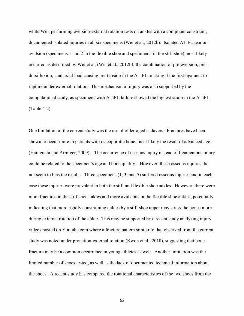
62

while Wei, performing eversion-external rotation tests on ankles with a compliant constraint,

documented isolated injuries in all six specimens (Wei et al., 2012b). Isolated ATiFL tear or

avulsion (specimens 1 and 2 in the flexible shoe and specimen 5 in the stiff shoe) most likely

occurred as described by Wei et al. (Wei et al., 2012b): the combination of pre-eversion, pre-

dorsiflexion, and axial load causing pre-tension in the ATiFL, making it the first ligament to

rupture under external rotation. This mechanism of injury was also supported by the

computational study, as specimens with ATiFL failure showed the highest strain in the ATiFL

(Table 4-2).

One limitation of the current study was the use of older-aged cadavers. Fractures have been

shown to occur more in patients with osteoporotic bone, most likely the result of advanced age

(Haraguchi and Armiger, 2009). The occurrence of osseous injury instead of ligamentous injury

could be related to the specimen’s age and bone quality. However, these osseous injuries did

not seem to bias the results. Three specimens (1, 3, and 5) suffered osseous injuries and in each

case these injuries were prevalent in both the stiff and flexible shoe ankles. However, there were

more fractures in the stiff shoe ankles and more avulsions in the flexible shoe ankles, potentially

indicating that more rigidly constraining ankles by a stiff shoe upper may stress the bones more

during external rotation of the ankle. This may be supported by a recent study analyzing injury

videos posted on Youtube.com where a fracture pattern similar to that observed from the current

study was noted under pronation-external rotation (Kwon et al., 2010), suggesting that bone

fracture may be a common occurrence in young athletes as well. Another limitation was the

limited number of shoes tested, as well as the lack of documented technical information about

the shoes. A recent study has compared the rotational characteristics of the two shoes from the

63

current studies with other shoes (Wei et al., 2012a), but future studies may want to look at more

shoes (it is important to note that a constant 1500 N axial load was applied to a surrogate ankle

during this stiffness testing, and different axial loads may result in different rotational

stiffnesses). Furthermore, technical characteristics of the shoes, besides rotational stiffness,

were not documented, and these could have an impact on talocrural joint motion and subsequent

injuries that were generated in these experiments. Future studies may want to document

additional differences in shoe construction that may have an effect on talocrural joint motion.

Additionally, the effect of muscle action was not included, which, on top of the specimen age,

may have been a limitation when attempting to reproduce the physiological behavior during an

actual sports injury. Yet, while it has been previously suggested that human subjects generate

10-20% more ankle joint torque than cadavers during sub-injurious external rotation (Wei et al.,

2011c), the magnitude of torque at failure was of little importance to the current study.

Furthermore, the proprioceptive muscle response is often too slow to have an effect on joint

motion during injury (Dubin et al., 2011, Delahunt et al., 2006), so it is likely that biomechanics

of the joint would differ only slightly during in vivo loading. Lastly, the small number of

specimens has an effect on reducing the statistical power of the study. Increasing the sample size

may have improved the robustness of the conclusions: more noted differences could possibly be

seen in talocrural rotation/degree of tibia rotation as well as differences in complex injury

frequency. However, the sample size was adequate to see differences in eversion, as well as key

ligament strains at failure.

64

In conclusion, the current study investigated ankle injury risk and its severity under combined

dorsiflexion, eversion, and external rotation while in either an American football shoe with a

relatively stiff or flexible upper design. Results of the study indicated that more talus eversion

occurred in flexible shoes under external rotation of the shoe, potentially allowing for a more

‘natural’ response of the ankle to rotation. As a result, the ankles in flexible shoes required

slightly more torque to fail and had fewer cases of complex ankle injury. Computational models

of the experiments showed that the response of the ankle to external rotation in a more flexible

shoe strained more ligaments than in a stiff shoe, but at more moderate levels. However, as

conclusions from this study only apply to external rotation of the ankle future studies may want

to investigate the performance characteristics of stiff versus flexible shoes in a variety of

circumstances in order to best recommend footwear that optimizes injury mitigation. In

addition, future studies may want to investigate the effect of shoe stiffness on joint kinematics in

regards to performance as well as injury, as previously studied with soccer shoes (Hennig, 2011).

The current study may help drive research and design of future American football shoes in order

to help limit injury risk without compromising the athlete’s comfort and performance.

65

CHAPTER 5:

THE EFFECT OF ROTATIONAL STIFFNESS ON ANKLE JOINT MOTION AND

LIGAMENT STRAIN DURING EXTERNAL ROTATION

ABSTRACT

The rotational stiffness of footwear has been previously shown to have an effect on ankle joint

kinematics and injury risk, but this relationship has not yet been quantified. The purpose of the

current study was to derive equations that could be used to predict ankle joint kinematics based

on the amount of ankle constraint. Three athletic tapes were tested for their ability to constrain

the ankle joint during external rotation. Six subjects then performed a voluntary external foot

rotation using the selected tape designs to constrain the ankle, as well as an unconstrained case.

Motion capture was performed to track the motion of the hindfoot with respect to the tibia (ankle

joint) up to fifteen degrees of tibia rotation and predictive equations were determined to establish

ankle joint rotation, eversion, and flexion as a function of gross tibia motion and tape stiffness.

These predictive equations were then used to drive a computational model in which ankle

ligament strains were determined at 15 degrees of tibia rotation and for ankle constraint stiffness

ranging from 0 Nm/deg to 30 Nm/deg. The three tapes provided significantly different

constraint stiffness during external foot rotation. There was no statistical effect of ankle joint

constraint on the dorsiflexion response of the ankle (p=0.461). In contrast, there was an effect of

constraint stiffness on ankle joint external rotation (p<0.001) and ankle joint eversion (p<0.001).

Results of the model simulation revealed the highest ligament strains in the anterior tibiotalar

ligament (ATiTL) and anterior tibiofibular ligament (ATiFL). ATiTL strain increased with

increasing constraint stiffness, while there was little effect of constraint stiffness on ATiFL

strain. Results from this study could aid in the design of footwear, as well as the analysis of

clinical injuries.

66

INTRODUCTION

External rotation of the foot with respect to the body is known to result in both medial and

syndesmotic ankle sprains and fractures (Waterman et al., 2011, Boytim et al., 1991, Haraguchi

and Armiger, 2009). Medial ankle injury involves damage to the anterior tibiotalar ligament

(ATiTL) (Wolfe et al., 2001), while syndesmotic (or high) ankle injury involves damage

primarily to the anterior tibiofibular ligament (ATiFL) (Dattani et al., 2008). These injuries are

most prevalent in contact sports where the injury mechanism is frequently attributed to a foot

being planted on the playing surface with internal rotation of the upper body (Guise, 1976).

While both injuries have been shown to involve some combination of external rotation,

dorsiflexion, and eversion (Waterman et al., 2010, Gerber et al., 1998, Norkus and Floyd, 2001,

Wei et al., 2012b), understanding more precisely the joint kinematics at the point of failure is an

important aspect for preventing injury.

Previous researchers have examined joint motion during medial and high ankle sprains using a

variety of techniques. One study used a rigid-body ankle model to investigate the effect of

different levels of joint eversion and dorsiflexion on ATiFL and ATiTL injury risk (Wei et al.,

2011a). Conclusions from this computational study motivated a cadaver study in which pairs of

ankles were rotated to failure in either an everted or neutral configuration, producing

syndesmotic and medial ankle sprains, respectively (Wei et al., 2012b). Results of both studies

concluded that the amount of eversion is critical in producing a syndesmotic versus a medial

ankle sprain. Yet, to provide a more complete understanding of external rotation injuries

occurring on the field, an in depth analysis of in vivo injuries may be warranted.

67

Krosshaug and colleagues have developed a model-based image matching (MBIM) motion

analysis technique to analyze three-dimensional human motion in an un-calibrated environment

using panning cameras (Krosshaug and Bahr, 2005). This technique was used to investigate two

cases of inversion ankle injury from the 2008 Beijing Olympics (Mok et al., 2011) and five cases

of inversion sprains in tennis (Fong et al., 2012). Results from these studies have provided new

information regarding the mechanism of lateral ankle sprain and have led to recommendations

for prevention of such sprains. However, accurate estimations of actual foot motion inside shoes

remains challenging.

In external rotation injuries motion of the ankle joint has been considered to play an important

role in generating ligament strains, particularly to the ATiTL and ATiFL (Sarsam and Hughes,

1988, Wei et al., 2011d). Therefore, in order to use MBIM to study external rotation injuries the

analysis would need to accurately quantify ankle joint motion. Previous studies from this lab,

however, have shown that ankle joint motion during upper body (tibial) rotation and the

subsequently generated injuries are highly dependent on rotational stiffness of the shoe (Wei et

al., 2012a). In order to analyze injurious scenarios or model the effect of different shoe

rotational stiffness, the relationship between constraint stiffness and ankle joint motion needs to

be investigated in more detail.

The purposes of the current study were (1) to have human subjects perform ankle external

rotation while constraining the foot with athletic tapes of different rotational stiffness (as a means

of determining the potential role of shoe stiffness on ankle motion) (2) to develop equations

relating the effect of constraint stiffness on 3D ankle motion, and finally (3) to use these

68

equations to drive a computational model to estimate the range of ligament strains that are

generated over a domain of constraint stiffness representative of various levels of shoe rotational

stiffness. It was hypothesized that taped constraint of the ankle would have a significant effect

on the amount of ankle joint motion during external rotation of the foot with respect to the upper

body, and that the effect on ankle joint kinematics would generate differences in key ligament

strains during external foot rotation. Information from this study may help investigators better

estimate ankle motion within various shoe designs and improve theoretical predictions of the

potential for ankle injuries during field conditions in order to optimize athletic footwear design

for preventing external rotation injuries of the ankle.

69

Figure 5-1 The surrogate ankle taped to the polycarbonate plate using Elastikon (a), PowerFlex

(b), and Sher-Light (c).

METHODS

Tape stiffness tests

Three athletic tapes were evaluated to determine their rotational stiffness properties for the ankle.

The experiments were conducted on a custom, hydraulic, biaxial testing machine with a 244 Nm

rotary actuator (Model SS-001-1V, Micromatic, Berne, MN) and a vertically oriented linear

70

actuator (Model 204.53, MTS Corp., Eden Praire, MN). The tapes evaluated in the study were

Andover PowerFlex, Covidien Sher-Light, and Johnson & Johnson Elasikon. The tapes

constrained a surrogate lower extremity made from room temperature curing epoxy resin (Fiber

Strand, Martin Senior Corp., Cleveland, OH) to a polycarbonate plate (32 cm x 8 cm) (Figure 5-

1). The taping was performed by an athletic training student (PT) with the goal of modelling the

constraint provided by a football shoe upper by applying two medial and two lateral heel locks.

The polycarbonate plate was clamped to a customized fixture that allowed x-y adjustments to

align the surrogate shank with the linear and torsional actuators. The proximal end of the

surrogate limb was inserted into an aluminum box which was attached to a rotary actuator

through a biaxial load cell (Model 1216CEW-2K, Interface, Scottsdale, AZ) with a capacity of

8896 N axial force and 113 Nm torsion (Figure 5-2).

Figure 5-2 The surrogate limb was attached to the testing machine

71

The axial load was zeroed and a rotational pre-torque of 2 Nm was applied to the surrogate foot

prior to internal rotation of the shank (external ankle rotation). The pre-torque was applied to

ensure tape contact on the medial side of the foot. A dynamic torque of 50 Nm was input in load

control at a frequency of 1 Hz (0.5 s to peak torque) and repeated six times for each tape. The

loading portion of the torque-rotation curve was averaged across the final five cycles of loading.

The slope of the linear portion of the curve (between 10 Nm and 50 Nm) was determined to yield

a rotational stiffness for each tape in Nm/deg.

This procedure was repeated, but with the surrogate ankle constrained by shoe/cleat molds

instead of tapes, as previously described by Wei et al. (Wei et al., 2012a). The shoes tested were

the Nike Flyposite and Nike Air, the stiffest and most flexible shoes from a previous study,

respectively (Button et al., 2015). In order to accurately mimic the tape stiffness tests, the axial

load was zeroed prior to rotation, unlike the Wei study which applied a 1500N axial pre-load

load to simulate body weight. The procedure from the Wei study was deemed ineffective for the

tape study because of potential high levels of torsional friction between the surrogate ankle and

the polycarbonate plate.

Human subject tests

Institutional Review Board approval was obtained for these experiments. Kinematic data from

six young (age: 27.3 ± 4.6 years), male subjects (body weight: 77.5 ± 8.9 kg) with no history of

lower body injury were collected after obtaining informed consent. A six-camera Vicon MX

Motion Capture System (OMG plc. Oxford, UK) was used to capture motion data at 100 Hz.

Marker arrays were placed on the anterior portion of the tibia, approximately 10 cm distal to the

72

patella, and on the calcaneal tuberosity (Figure 5-3). Each subject’s right foot was measured

prior to testing and a polycarbonate plate was cut to fit. The subject’s right foot was taped to the

1/8” thick polycarbonate plate by the athletic trainer (PT) using two medial and two lateral heel

locks and one of three athletic tapes for each experiment. The foot/plate was adhered to the

ground using a Dycem adhesive sheet (Dycem Ltd, Warwick, RI, USA). The left foot was placed

adjacent to the right foot on a raised surface so the feet were level. The subject performed an

internal rotation of the body (external rotation of the foot) at a self-determined maximal effort,

trying to minimize tibia flexion and eversion. Each subject repeated this motion until 10

successful trials were collected. The procedure was repeated for each tape and under a tapeless

condition (note: the shoes were not used in the human subject tests).

Figure 5-3 Marker arrays were placed on the subject’s anterior tibia, about 10 cm distal to the

patella, and the calcaneal tuberosity.

73

Coordinate transformations were performed on the tibia and hindfoot marker arrays in order to

establish orthogonal coordinate systems in line with the three axes of the ankle (Figure 5-4). A

joint coordinate system (JCS) was then established between the tibia and hindfoot (henceforth

referred to as the ankle joint), similar to a previously defined system (Wu et al., 2002):

�� = �� (1a)

� = �� (1b)

�� =�� ×��

|�� ×��| (1c)

� = �� ∙ �� (flexion) (2a)

� = �� ∙ �� (rotation) (2b)

� = �� ∙ �� (inversion/eversion) (2c)

Calculations of absolute tibia rotation, eversion, and flexion with respect to the laboratory were

performed by the same method, but the JCS was established between the tibia coordinate system

and a fixed laboratory coordinate system aligned with the axes shown in Figure 5-4.

Calculations for ankle joint flexion, rotation, and inversion/eversion were determined over a

range of 0 to 15 degrees of tibia rotation.

74

Figure 5-4 Three orthogonal axes of the ankle. Rotations about these axes are described as

plantarflexion/dorsiflexion, eversion/inversion, and internal/external rotation.

Predictions of ankle joint dorsiflexion, eversion, and rotation were determined as a function of

tibia rotation, tibia eversion, tibia dorsiflexion, and tape stiffness. Irrelevant predictors and

interaction terms were eliminated by using the ‘stepwisefit’ and ‘LinearModel.fit’ functions,

respectively, in MATLAB.

Computational modelling

Predicted ankle joint motion data from the curve fitting equations were used to drive a generic

computational ankle model. Details of the model development and its validation have been

described in previous studies (Wei et al., 2011d, Button et al., 2013), so they will only be

described briefly here. The ankle model was based on a computed tomography (CT) scan of a

fresh frozen, right male cadaver foot (52 years old) showing no signs of abnormal anatomy.

Digital information from the scan was transferred from Digital Imaging and Communications in

75

Medicine (DICOM) files into Materialise’s Interactive Imaging Control System (MIMICS,

Leuven, Belgium) software. Three dimensional surface models of the bones, as

Stereolithography (STL) files, were created and exported to SolidWorks 2011 (Trimech

Solutions, LLC, Columbia, MD), where the bones were simplified and assembled. SolidWorks

Motion was used to add ligaments (modelled as linear springs) and insertion locations were

determined from previous dissections in this laboratory (KB and FW) and an anatomical atlas

(Netter and JT, 2003). A pre-load was induced in each ligament by reducing its length by 2%,

inducing in situ preloads (Liacouras and Waynel, 2007). The model has been previously

validated based on ankle ligament strain (Colville et al., 1990a), ankle joint torque (Wei et al.,

2010), talus rotation (Button et al., 2013), and injuries generated during external rotation

experiments (Button et al., 2013).

The motion simulation was run in displacement control with motors driving the three-

dimensional rotations of the tibia and talus. The input for the tibia motor was a ramp to 15

degrees of external rotation, with no eversion or dorsiflexion (modelling an isolated external

rotation). The talus rotation, eversion, and dorsiflexion (determined from results of ‘Curve

Fitting’ section) were dependent on the amount of tibia rotation at a given time point and the

rotational stiffness parameter. The forefoot was fixed while the calcaneus, talus, tibia, and fibula

were free to move. The body weight was simulated as an axial load on the proximal end of the

model with one-sixth of the loading on the fibula and the rest on the tibia (Wei et al., 2011d).

Ligament strains were determined during rotation.

76

Statistical analysis

One-way ANOVA and Tukey post-hoc tests were used to statistically determine differences in

rotational stiffness between tapes/shoes. Two-way repeated measures ANOVA and Tukey post-

hoc tests were used to statistically determine differences in ankle joint dorsiflexion, external

rotation, and eversion for the three tape (and no tape) designs (factor one) at each rotation level

(factor two). In all statistical tests, p-values less than 0.05 were considered significant.

RESULTS

The 2 Nm pre-load was zeroed out by shifting the torque-rotation curves, which showed nearly

linear behavior beyond 10 Nm of input torque (Figure 5-5a and b). The rotational stiffness of the

Elastikon, Sher-Light, and PowerFlex tapes were 25.7 ± 1.6 Nm/deg, 22.6 ± 0.75 Nm/deg, and

13.5 ± 0.37 Nm/deg, respectively. The rotational stiffness of the Air and Flyposite shoes were

16.5 ± 0.44 Nm/deg and 25.8 ± 1.1 Nm/deg, respectively. There were significant differences

between all the tape/shoe designs, except between the Flyposite shoe and Elastikon tape

(p=0.99).

77

Figure 5-5 Torque-rotation curves for the three tape designs and two shoe designs from

rotational stiffness tests (a), and rotational stiffness values determined from the slopes of the

torque-rotation curves (b). Curves with different symbols (* # ƚ ¥) indicate statistically different

stiffness between designs.

a

b

78



between tape designs.

Figure 5-7 Mean ankle joint external rotation-tibia rotation curves for the three tape (and no-

tape) designs from an in vivo external foot rotation (n=6). Different symbols (* # ƚ ǂ) indicate

statistically different curves.

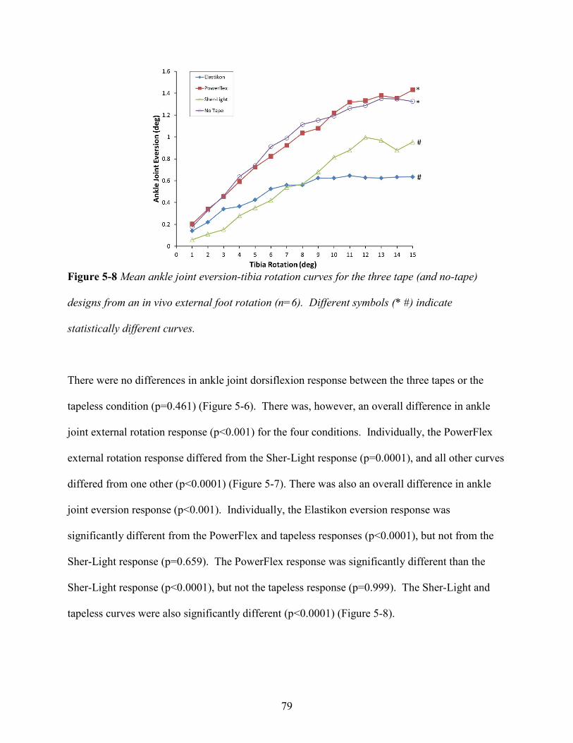
79

Figure 5-8 Mean ankle joint eversion-tibia rotation curves for the three tape (and no-tape)

designs from an in vivo external foot rotation (n=6). Different symbols (* #) indicate

statistically different curves.

There were no differences in ankle joint dorsiflexion response between the three tapes or the

tapeless condition (p=0.461) (Figure 5-6). There was, however, an overall difference in ankle

joint external rotation response (p<0.001) for the four conditions. Individually, the PowerFlex

external rotation response differed from the Sher-Light response (p=0.0001), and all other curves

differed from one other (p<0.0001) (Figure 5-7). There was also an overall difference in ankle

joint eversion response (p<0.001). Individually, the Elastikon eversion response was

significantly different from the PowerFlex and tapeless responses (p<0.0001), but not from the

Sher-Light response (p=0.659). The PowerFlex response was significantly different than the

Sher-Light response (p<0.0001), but not the tapeless response (p=0.999). The Sher-Light and

tapeless curves were also significantly different (p<0.0001) (Figure 5-8).

80

Predictive equations for ankle joint dorsiflexion (AJDorsi), ankle joint rotation (AJRot), and

ankle joint eversion (AJever) as a function of tibia dorsiflexion (TIdorsi), tibia rotation (TIrot),

tibia eversion (TIever), and tape stiffness (Stiff) are shown in equations 3a-c with correlation

coefficients 0.99, 0.99, and 0.95, respectively.

AJdorsi = 0.0343 + 0.6794 ∗ �./01�� (3a)

AJrot = 0.29551 + 0.6804 ∗ �.107 + 87�99�0.0089 ∗ �.107 − 0.0099� (3b)

AJever = 0.11525 + 0.4209 ∗ �.�=�1 + 0.08371 ∗ �.107 − 87�99�0.0024 ∗ �.107 + 0.0007 ∗

87�99 + 0.0002� (3c)

External rotation of a neutral ankle strained the ATiFL and ATiTL the most. The effects of

ankle constraint stiffness on the ATiTL strain were greater than those on the ATiFL strain

(Figure 5-9a and b). Fifteen degrees of tibial rotation strained the ATiFL 15.5-16.2%, while the

ATiTL strain was between 6.7% and 14.5%. At 15 deg of tibial rotation, each increment of 5

Nm/deg in stiffness theoretically increased ATiTL strain approximately 1.2%.

81



0 to 30 Nm/deg. Inputs for ankle joint motion were based on predictive equations 3a-3c.

a

b

82

DISCUSSION

The current study investigated the effect of ankle constraint on the three-dimensional motion of

the ankle using different athletic tapes. Three tapes (and a no-tape condition) were used to

constrain human ankles during an in vivo voluntary external ankle rotation. The rotational

stiffness of the tapes was comparable to those of a relatively stiff and a compliant football shoe

design. Predictive equations for determining ankle joint motion as a function of tibia motion and

tape stiffness were developed from human subject testing results. These predictive equations

were used to drive a generic computational ankle model for the calculation of ligament strain

during isolated external ankle rotation. Results of the experimental study indicated that for a

given tibia rotation the amount of ankle joint eversion and external rotation was dependent on the

level of ankle constraint, with a stiffer ankle constraint allowing greater ankle rotation, but less

eversion. Constraint on the ankle also affected theoretical ligament strain: increasing constraint

stiffness substantially increased ATiTL strain, but had little effect on ATiFL strain. These

results supported the hypothesis that constraint stiffness would have a significant effect on ankle

joint eversion and rotation during foot external rotation.

Previous investigations on anatomical specimens conclude that external rotation of an

unconstrained ankle results in a combination of eversion and rotation (Lundberg et al., 1989b).

This potentially explains the increased eversion measured in ankles constrained with a more

flexible tape, likely because the applied rotation can be more easily transferred about other axes

of the ankle. In particular, less constraint of the subtalar and transverse tarsal joints may allow

more motion between the talus and calcaneus, generating foot eversion (Hertel et al., 1999, Wei

et al., 2012a). With increased tape stiffness, however, this natural response was restricted,

83

resulting in nearly isolated ankle external rotation. Additionally, while eversion and external

rotation are strongly coupled, they are only weakly coupled with dorsiflexion (Lundberg et al.,

1989b), potentially explaining why ankle dorsiflexion was only a function of absolute tibia

dorsiflexion (Equation 3a). The apparent correlation between tibia rotation and ankle joint

dorsiflexion noted in Figure 5-6 was most likely due to an increased tibia flexion that occurred as

a result of loading the leg.

Foot external rotation primarily strained the ATiTL and ATiFL in the computational model.

Figure 5-9 shows that axial load put an ~8% pre-strain on the ATiFL, likely due to the

tibiofibular syndesmosis opening slightly around the talus upon contact. External rotation put

additional strain on the ligament, and constraint stiffness had little effect on strain magnitude.

However, increasing constraint stiffness correlated with considerable increases in ATiTL strain.

Unlike the ATiFL, the ATiTL strain did not increase with axial load, but increased linearly with

tibia rotation once the ligament began to tense around 5-7° of tibia rotation. The observation of

increased ATiTL strain with increasing rotational ankle constraint suggested that a stiffer

constraint may predispose the ankle to medial ankle injury during external rotation. This

potentially explains the results from a previous cadaver study in which pairs of cadaver ankles

were rotated to failure in either a stiff (Flyposite) or flexible (Air) football shoe. A high

frequency of combination medial and syndesmotic ankle injuries were noted in the stiff shoes,

while ankles in flexible shoes mostly suffered islolated syndesmotic injuries (Button et al.,

2015).

84

The information regarding the effect of ankle constraint on ankle joint kinematics and injury risk

may benefit the future design of athletic shoes. Previous studies have examined the effects of

running shoe structure (Bonacci et al., 2013, Peltz et al., 2014, Williams et al., 2012) and football

shoes (Wei et al., 2012a, Button et al., 2015), as well as the effects of shoe-surface interface

(Villwock et al., 2009a) on joint kinematics and injury risk, but no study has quantified and

modelled these effects. Two shoe designs from a previous cadaver study (Wei et al., 2012a,

Button et al., 2015) were subjected to rotational stiffness testing in order to assess whether or not

the constraint offered by the athletic tapes was a realistic simulation of athletic footwear (Figure

5-5). It was noted that the stiffer shoe (Nike Flyposite) behaved almost identically to the stiffest

tape (Elastikon), while the more flexible shoe (Nike Air) behaved between the moderate (Sher-

Light) and most flexible tape (PowerFlex). This indicated that the tapes used in this study

reasonably matched stiff and flexible shoe designs used in previously studies by this laboratory

during external rotation, but future studies may want to constrain in vivo or cadaver ankles with

different shoes instead of tapes to further investigate this effect.

Predictive equations derived in the current study may also help in the analysis of injury

mechanisms during athletic competition. Using Krosshaug’s MBIM technique to analyze leg

and shoe kinematics in game films, Fong et al. (Fong et al., 2012) and Mok et al. (Mok et al.,

2011) documented wide variations in the amount of joint motion at ligament failure, with peak

inversion values ranging from 48o to 148°. However, much of this disparity could be due to

different constraints on the ankle joint in different footwear. Predictive equations from the

current study exhibited that 15 degrees of isolated tibia rotation could result in 10.5o-14.2° of

ankle joint rotation and 6.7-14.2% ATiTL strain, depending on ankle constraint. Future studies

85

may want to not only use MBIM to investigate the kinematics of the leg with respect to the shoe

during external rotation, but complement this information with the known rotational shoe

stiffness-ankle motion relationships to more accurately assess ankle joint kinematics inside the

shoe. Such information, combined with cadaver studies and computational modeling, could help

provide researchers with a more complete understanding of ankle kinematics within the shoes

during high and medial ankle sprains.

While the current study utilized human subjects, future studies may benefit from studying joint

motion under various constraints using cadaver specimens. While in vivo studies rely largely on

voluntary motions, using cadaver specimens would allow more precise control of input motions.

Reflective markers could also be screwed into the talus, calcaneus, and tibia. Marker arrays on

both the talus and calcaneus would enable the calculation of both subtalar and talocrural joint

kinematics. Additionally, using screw-in marker sets instead of skin marker sets could

potentially mitigate any errors associated with skin motion. Furthermore, a limitation of the

current study was that the analysis was restricted to sub-failure rotations. Using cadavers could

allow researchers to measure ankle kinematics and ligament behavior at failure-level foot

rotations, which may differ from sub-failure behavior. Comparing results from a cadaver study

with an in vivo study could also help quantify the effect of muscle action on ankle joint

kinematics during external foot rotation.

In conclusion, the current study quantified the effect of constraint on ankle joint motion during

voluntary external foot rotation. The study showed that constraint of the ankle had an effect on

the amount of ankle eversion and rotation for a given degree of tibia rotation, while dorsiflexion

was unaffected. A computational model of the ankle and its major ligamentous structures

86

showed that ATiTL strain was highly dependent on ankle constraint, while ATiFL strain was not.

The current study represents an important step in understanding the effect of different footwear

on ankle joint kinematics during external rotation of the foot relative to the upper body.

87

CHAPTER 6:

A METHOD OF DETERMINING IN VIVO DYNAMIC HUMAN ANKLE STIFFNESS

DURING EXTERNAL ROTATION

ABSTRACT

This study presents a method to determine stiffness of the human ankle in internal-external

rotation, inversion-eversion, and plantarflexion-dorsiflexion during an in vivo, single-legged,

external foot rotation experiment. Five young male subjects stood on one foot and performed an

internal rotation of the body (external rotation of the foot) on a force plate, while motions were

captured with a motion capture system. Hindfoot rotations relative to the tibia and resistive

moments in the above three directions were obtained using a commercial software package. The

resistive moments were plotted against rotation during the loading portions of the curves. Linear

approximations of these curves were used to determine stiffness of the ankle in directions of

internal-external, inversion-eversion, and plantarflexion-dorsiflexion. Future data from the above

experiment and other athletic motions may be useful for the design of surrogate devices used to

evaluate the potential performance and ankle injury risk characteristics of various shoe-surface

interfaces.

INTRODUCTION

Acute ankle trauma accounts for 10-30% of sports-related injuries (Hootman et al., 2007). While

medial and high ankle sprains are less common than lateral ankle sprains, they represent a more

disabling problem requiring longer recovery times (Wolfe et al., 2001). Preventative measures

may require the assessment of current footwear and playing surfaces.

88

The mechanism of medial and high ankle sprains has been clinically ascribed to excessive

external foot rotation (Guise, 1976, Boytim et al., 1991). Additionally, foot eversion prior to

external rotation has been shown critical in generating a high ankle sprain(Wei et al., 2012b). It

is also generally accepted that excessive rotational traction (Cawley et al., 2003) at the shoe-

surface interface may precipitate ankle and knee injuries (Nigg and Yeadon, 1987). Livesay et al.

(Livesay et al., 2006) suggest that rotational stiffness of the shoe-surface interface may be a more

important parameter than torque in determining ankle injury risk. Thus, evaluations of shoe-

surface interface with devices and development of preventative measures should use surrogate

ankles that have appropriate 3D properties and can simulate motions of the human ankle.

Previous studies documenting human ankle stiffness (or compliance) have determined ankle

stiffness using controlled input motions (Villwock et al., 2009c, Petit, 1996, Crandall et al.,

1996). However, little information exists on motions of the human ankle and its stiffness during

voluntary athletic maneuvers. The objective of the current study was to describe a method that

integrates experimentally obtained kinematic and kinetic data to produce useful structural

characteristics of the in vivo, human ankle during external foot rotation. This information may

help in the future development of surrogate devices to assess performance and ankle injury risk

characteristics of shoe-surface interfaces.

89

Figure 6-1 Marker set of the Oxford Foot Model (Carson et al., 2001). The subjects stood on

one foot and performed an internal rotation of the body (external rotation of the foot).

METHODS

Institutional Review Board approval was obtained for this project. In vivo kinematic data were

collected after obtaining informed consent from five young, male subjects with body mass of

77.9 ± 18 kg. A six-camera Vicon MX Motion Capture System (OMG plc. Oxford, UK) was

used to capture motions at 100 Hz from a marker set defined by the Oxford Foot Model (OFM)

(OMG plc., Oxford, UK) (Carson et al., 2001). An AMTI (Advanced Mechanical Technology,

Inc., Watertown, MA) force plate was used to capture ground reaction data at 1000 Hz. The

subjects stood with a flexed right leg on the force plate, balanced themselves, and performed an

internal rotation of the body (external rotation of the foot) with a self-determined maximum

effort (Figure 6-1). The subjects were instructed to internally rotate their bodies at a self-selected

speed, but within 3s, while keeping their foot on the force plate. Data were acquired over four

90

trials and processed using commercial kinetic (Plug-in Gait, OMG plc., Oxford, UK) and

kinematic (Dynamic OFM) software packages.

Figure 6-2 Sample of a moment versus time plot (left) and rotation versus time plot (right) for all

three movements: internal-external rotation, inversion-eversion, and plantarflexion-dorsiflexion.

Data from the loading phase (shaded in the figure) for moment vs. time were extracted and

plotted against the extracted rotation vs. time data, as shown in Figure 6-3.

Hindfoot rotations relative to the tibia and the corresponding resistive moments of the ankle in

three directions were obtained from the Plug-in Gait package. The moments were measured with

respect to the center of the ankle joint, as determined by the Plug-in Gait package. Moment and

rotation versus time plots were generated from the trials of each subject (Figure 6-2). The three

dimensional moments were plotted against the corresponding rotations from the beginning of

ankle loading (either a peak or sink in the response curve) to the end of loading (another peak or

sink). A linear regression was performed on the moment-rotation plot in order to determine the

slope and coefficient of determination (R2) for each trial. The average slope of the four trials

from each subject was used to represent subject ankle stiffness (Figure 6-3).

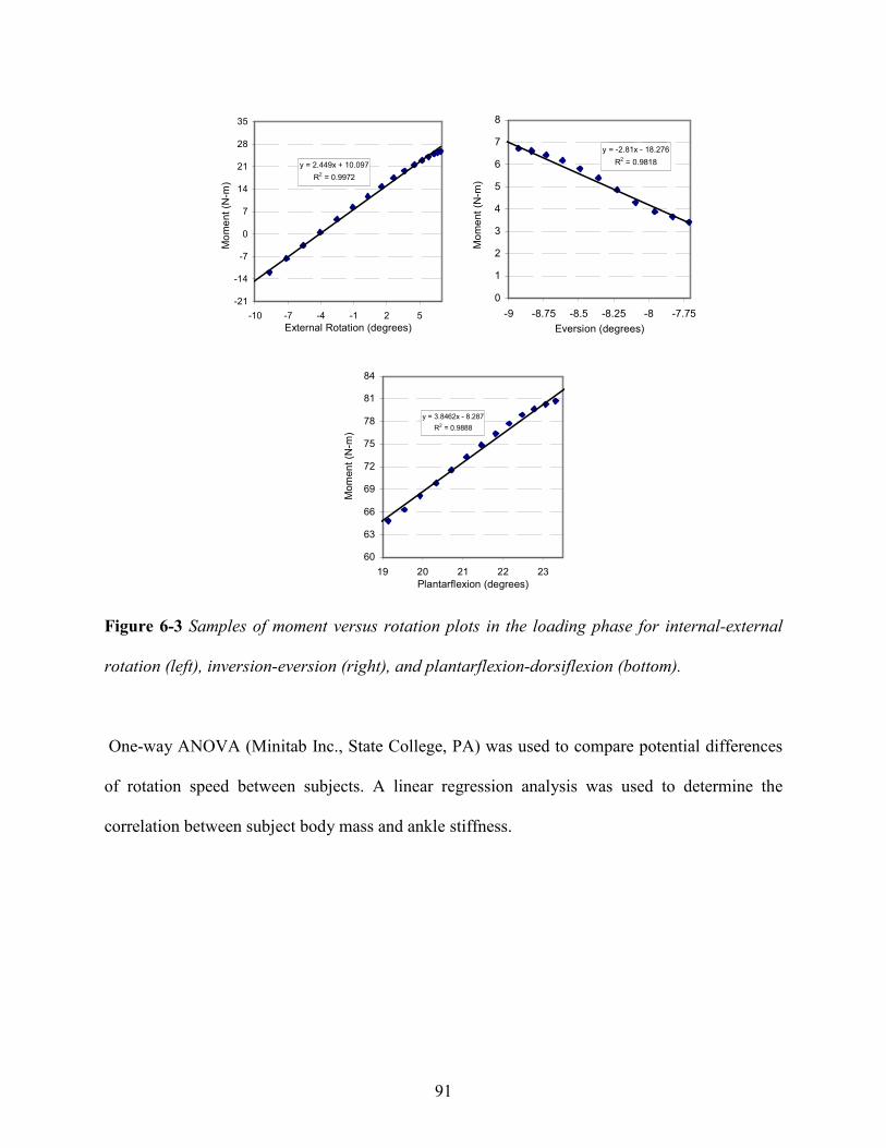
91

Figure 6-3 Samples of moment versus rotation plots in the loading phase for internal-external

rotation (left), inversion-eversion (right), and plantarflexion-dorsiflexion (bottom).

One-way ANOVA (Minitab Inc., State College, PA) was used to compare potential differences

of rotation speed between subjects. A linear regression analysis was used to determine the

correlation between subject body mass and ankle stiffness.

y = 2.449x + 10.097

R2 = 0.9972

-21

-14

-7

0

7

14

21

28

35

-10 -7 -4 -1 2 5

External Rotation (degrees)

Mo

me

nt

(N-m

)

y = -2.81x - 18.276

R2 = 0.9818

0

1

2

3

4

5

6

7

8

-9 -8.75 -8.5 -8.25 -8 -7.75

Eversion (degrees)

Mo

me

nt

(N-m

)

.

y = 3.8462x - 8.287

R2 = 0.9888

60

63

66

69

72

75

78

81

84

19 20 21 22 23

Plantarflexion (degrees)

Mom

en

t (N

-m)

92

Table 6-1 Ankle stiffnesses in three directions obtained from subjects performing a single legged external rotation of the foot with

standard deviations in parenthesis. Note: the absolute value of the inversion-eversion slope was taken so that the reported number

was positive.

1 2 3 4 5

52.47 (23.63) 75.20 (19.07) 61.83 (15.65) 43.00 (11.49) 86.21 (16.51) 63.75 17.3

0.93 0.04R2 0.89 (0.14) 0.89 (0.08) 0.99 (0.01) 0.92 (0.04) 0.97 (0.04)

4.31

Range (deg) 0.72 (0.35) 4.54 (1.28) 3.27 (0.23) 2.77 (2.21) 2.11 (0.95) 2.68 1.41

0.97 0.02

Plantarflexion/dorsiflexion

Stiffness (Nm/deg) 12.13 (0.08) 3.47 (1.13) 8.05 (1.60) 2.20 (0.53) 2.50 (1.07) 5.68

R2 0.99 (0.00) 0.96 (0.05) 0.95 (0.05) 0.98† 0.98 (0.01)

0.72

Range (deg) 6.72 (3.78) 2.77 (1.56) 1.03 (0.50) 4.14† 1.37 (0.43) 3.2 2.32

0.99 0.01

Inversion/eversion

Stiffness (Nm/deg) 0.71 (0.35) 1.67 (1.05) 2.13 (0.92) 2.08† 2.64 (.28) 1.85

R2 0.98 (0.00) 0.99 (0.01) 0.99 (0.00) 0.98 (0.02) 0.99 (0.00)

2.19 0.52

Range (deg) 11.87 (6.69) 18.41 (5.78) 14.69 (4.98) 5.93 (1.00) 23.69 (4.84) 14.92 6.69

Mean SD

Rotation Speed (deg/s)

Internal/external rotation

Stiffness (Nm/deg) 1.80 (0.86) 1.52 (0.23) 2.67 (1.03) 2.65 (0.65) 2.31 (0.04)

Subject

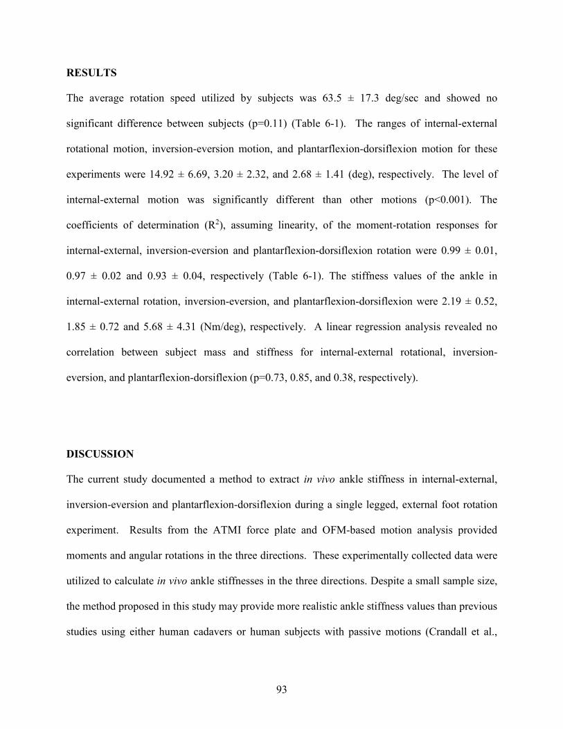
93

RESULTS

The average rotation speed utilized by subjects was 63.5 ± 17.3 deg/sec and showed no

significant difference between subjects (p=0.11) (Table 6-1). The ranges of internal-external

rotational motion, inversion-eversion motion, and plantarflexion-dorsiflexion motion for these

experiments were 14.92 ± 6.69, 3.20 ± 2.32, and 2.68 ± 1.41 (deg), respectively. The level of

internal-external motion was significantly different than other motions (p<0.001). The

coefficients of determination (R2), assuming linearity, of the moment-rotation responses for

internal-external, inversion-eversion and plantarflexion-dorsiflexion rotation were 0.99 ± 0.01,

0.97 ± 0.02 and 0.93 ± 0.04, respectively (Table 6-1). The stiffness values of the ankle in

internal-external rotation, inversion-eversion, and plantarflexion-dorsiflexion were 2.19 ± 0.52,

1.85 ± 0.72 and 5.68 ± 4.31 (Nm/deg), respectively. A linear regression analysis revealed no

correlation between subject mass and stiffness for internal-external rotational, inversion-

eversion, and plantarflexion-dorsiflexion (p=0.73, 0.85, and 0.38, respectively).

DISCUSSION

The current study documented a method to extract in vivo ankle stiffness in internal-external,

inversion-eversion and plantarflexion-dorsiflexion during a single legged, external foot rotation

experiment. Results from the ATMI force plate and OFM-based motion analysis provided

moments and angular rotations in the three directions. These experimentally collected data were

utilized to calculate in vivo ankle stiffnesses in the three directions. Despite a small sample size,

the method proposed in this study may provide more realistic ankle stiffness values than previous

studies using either human cadavers or human subjects with passive motions (Crandall et al.,

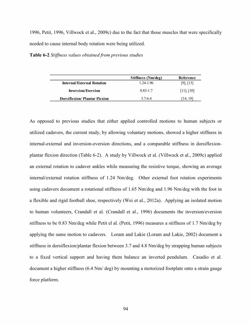
94

1996, Petit, 1996, Villwock et al., 2009c) due to the fact that those muscles that were specifically

needed to cause internal body rotation were being utilized.

Table 6-2 Stiffness values obtained from previous studies

As opposed to previous studies that either applied controlled motions to human subjects or

utilized cadavers, the current study, by allowing voluntary motions, showed a higher stiffness in

internal-external and inversion-eversion directions, and a comparable stiffness in dorsiflexion-

plantar flexion direction (Table 6-2). A study by Villwock et al. (Villwock et al., 2009c) applied

an external rotation to cadaver ankles while measuring the resistive torque, showing an average

internal/external rotation stiffness of 1.24 Nm/deg. Other external foot rotation experiments

using cadavers document a rotational stiffness of 1.65 Nm/deg and 1.96 Nm/deg with the foot in

a flexible and rigid football shoe, respectively (Wei et al., 2012a). Applying an isolated motion

to human volunteers, Crandall et al. (Crandall et al., 1996) documents the inversion/eversion

stiffness to be 0.83 Nm/deg while Petit el al. (Petit, 1996) measures a stiffness of 1.7 Nm/deg by

applying the same motion to cadavers. Loram and Lakie (Loram and Lakie, 2002) document a

stiffness in dorsiflexion/plantar flexion between 3.7 and 4.8 Nm/deg by strapping human subjects

to a fixed vertical support and having them balance an inverted pendulum. Casadio et al.

document a higher stiffness (6.4 Nm/ deg) by mounting a motorized footplate onto a strain gauge

force platform.

Stiffness (Nm/deg) Reference

Internal/External Rotation 1.24-1.96 [9], [13]

Dorsiflexion/ Plantar Flexion 3.7-6.4 [14, 19]

Inversion/Eversion 0.83-1.7 [11], [10]

95

One limitation of the current study was that subjects generated internal rotation of their bodies

with only a small amount of initial plantar-dorsiflexion or inversion-eversion rotation, resulting

in fewer data points. A previous study by Smith and Wong (Smith and Wong, 2012) has noted

that, when calculating ankle stiffness, more data points result in a higher reliability. Future

studies may have to adjust sampling rate in order to increase data reliability. Another limitation

of the current study was that ankle stiffness was determined in only the voluntary range of

loading. Previous cadaver studies (Villwock et al., 2009c, Petit, 1996, Crandall et al., 1996) have

noted a bilinear stiffness response of the ankle, with the stiffness increasing near failure levels.

It, of course, was not possible to conduct the current in vivo studies at high levels of internal

body rotation due to human subject safety issues. However, by comparing data from subfailure

in vivo and cadaver studies, the role of ankle musculature may be estimated by the use of a

mathematical model, similar to that utilized in a glenohumeral joint study by Elmore and Wayne

(Elmore KA, 2012) and the ankle study by Wei et al. (Wei et al., 2011d) (without musculature

effects). Based on such approximations, a surrogate ankle may be constructed that might yield a

better tool to determine the roles of various shoe-surface-interfaces on athletic performance and

their potential in producing high ankle sprains. Finally, a limitation of all studies involving

human subjects is the potential for variances in subject performance, particularly evident in the

ranges of motion during external rotation This is likely a result of the complex anatomy of the

talocrural joint which can result in differences in range of motion (and thus loading time) due to

differences in bone shape and spacing. As a result, while we believe in vivo data are most

appropriate for evaluations of shoe-surface interface characteristics, future studies may need to

provide better control of subject motions and very likely involve a large number of human

participants to generate reliable ankle stiffness information for the development of a biofidelic

96

surrogate device. Additionally, more trials from each subject could be taken in order to test the

repeatability of the current data.

While the current study was limited to internal rotation of the body with the foot planted on a

force plate, the methodology for determining ankle stiffness could be utilized in studies of other

athletic maneuvers, such as external rotation of the body with a planted foot or for various

cutting maneuvers. The current study utilized motion capture and a force plate to accomplish

this, but future studies might also utilize pressure insoles to help determine ankle stiffness during

more complex motions outside the laboratory (Weaver et al., 2013). Such data could more

completely characterize human ankle stiffness under a variety of situations on the athletic field.

These data may then be useful for the development of future surrogate test devices to evaluate

potential athletic performance and ankle injury risk characteristics of shoe-surface interfaces.

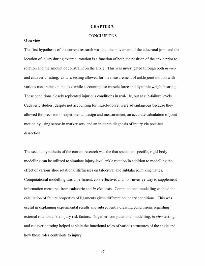
97

CHAPTER 7:

CONCLUSIONS

Overview

The first hypothesis of the current research was that the movement of the talocrural joint and the

location of injury during external rotation is a function of both the position of the ankle prior to

rotation and the amount of constraint on the ankle. This was investigated through both in vivo

and cadaveric testing. In vivo testing allowed for the measurement of ankle joint motion with

various constraints on the foot while accounting for muscle force and dynamic weight bearing.

These conditions closely replicated injurious conditions in real-life, but at sub-failure levels.

Cadaveric studies, despite not accounting for muscle-force, were advantageous because they

allowed for precision in experimental design and measurement, an accurate calculation of joint

motion by using screw-in marker sets, and an in-depth diagnosis of injury via post-test

dissection.

The second hypothesis of the current research was the that specimen-specific, rigid-body

modelling can be utilized to simulate injury-level ankle rotation in addition to modelling the

effect of various shoe rotational stiffnesses on talocrural and subtalar joint kinematics.

Computational modelling was an efficient, cost-effective, and non-invasive way to supplement

information measured from cadaveric and in vivo tests. Computational modelling enabled the

calculation of failure properties of ligaments given different boundary conditions. This was

useful in explaining experimental results and subsequently drawing conclusions regarding

external rotation ankle injury risk factors. Together, computational modelling, in vivo testing,

and cadaveric testing helped explain the functional roles of various structures of the ankle and

how those roles contribute to injury.

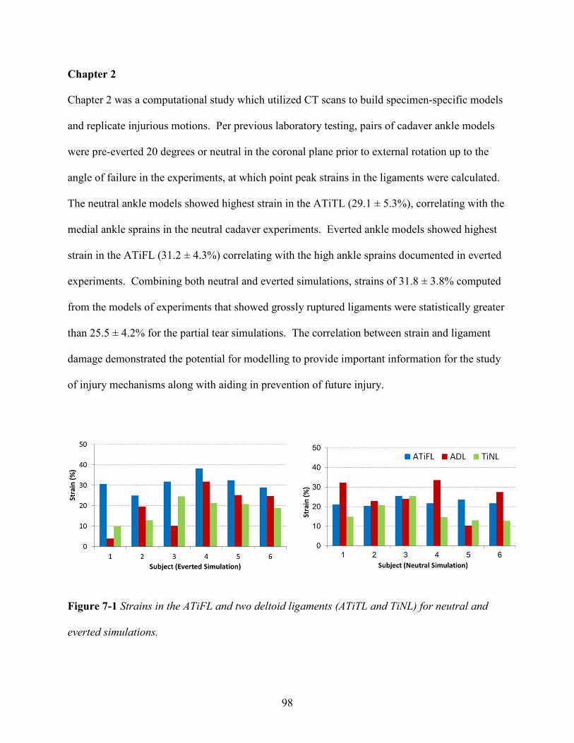
98

Chapter 2

Chapter 2 was a computational study which utilized CT scans to build specimen-specific models

and replicate injurious motions. Per previous laboratory testing, pairs of cadaver ankle models

were pre-everted 20 degrees or neutral in the coronal plane prior to external rotation up to the

angle of failure in the experiments, at which point peak strains in the ligaments were calculated.

The neutral ankle models showed highest strain in the ATiTL (29.1 ± 5.3%), correlating with the

medial ankle sprains in the neutral cadaver experiments. Everted ankle models showed highest

strain in the ATiFL (31.2 ± 4.3%) correlating with the high ankle sprains documented in everted

experiments. Combining both neutral and everted simulations, strains of 31.8 ± 3.8% computed

from the models of experiments that showed grossly ruptured ligaments were statistically greater

than 25.5 ± 4.2% for the partial tear simulations. The correlation between strain and ligament

damage demonstrated the potential for modelling to provide important information for the study

of injury mechanisms along with aiding in prevention of future injury.

Figure 7-1 Strains in the ATiFL and two deltoid ligaments (ATiTL and TiNL) for neutral and

everted simulations.

99

Chapter 3

Chapter 3 was an experimental study that investigated the effect of pre-eversion on talocrural and

subtalar joint motion during external rotation. Fourteen (seven pairs) cadaver lower extremities

were externally rotated 20 degrees in either a pre-everted or neutral configuration. Vicon motion

capture was used to track the motion of marker arrays on the tibia, talus, and calcaneus. Joint

coordinate systems between the tibia and talus (talocrural) and talus and calcaneus (subtalar)

were established to measure rotation, flexion, and in-eversion. While talocrural joint rotation

was greater in the neutral ankle (13.33 ± 2.09 deg versus 10.51 ± 2.75 deg, p=0.006), subtalar

joint rotation was greater in the pre-everted ankle (2.38 ± 1.89 deg versus 1.12 ± 1.04 deg,

p=0.014). Overall, the talocrural joint rotated more than the subtalar joint (11.92 ± 2.77 deg

versus 1.75 ± 1.61 degrees, p<0.001).

It was proposed that the calcaneus and talus ‘lock’ when axial load is applied to a neutral joint,

limiting subtalar motion, but maximizing talocrural rotation. When the foot is everted prior to

axial load, the subtalar joint may ‘unlock’ enabling the tibiotalar ligaments to pull the talus with

the rotation of the tibia, resulting in lower relative motion. This ‘unlocking’ of the subtalar joint

puts less strain on the medial ligaments potentially explaining why the combination of eversion

and external rotation does not always damage the anterior deltoid. This study may improve our

understanding of various mechanisms of ankle injury during external rotation of the foot.

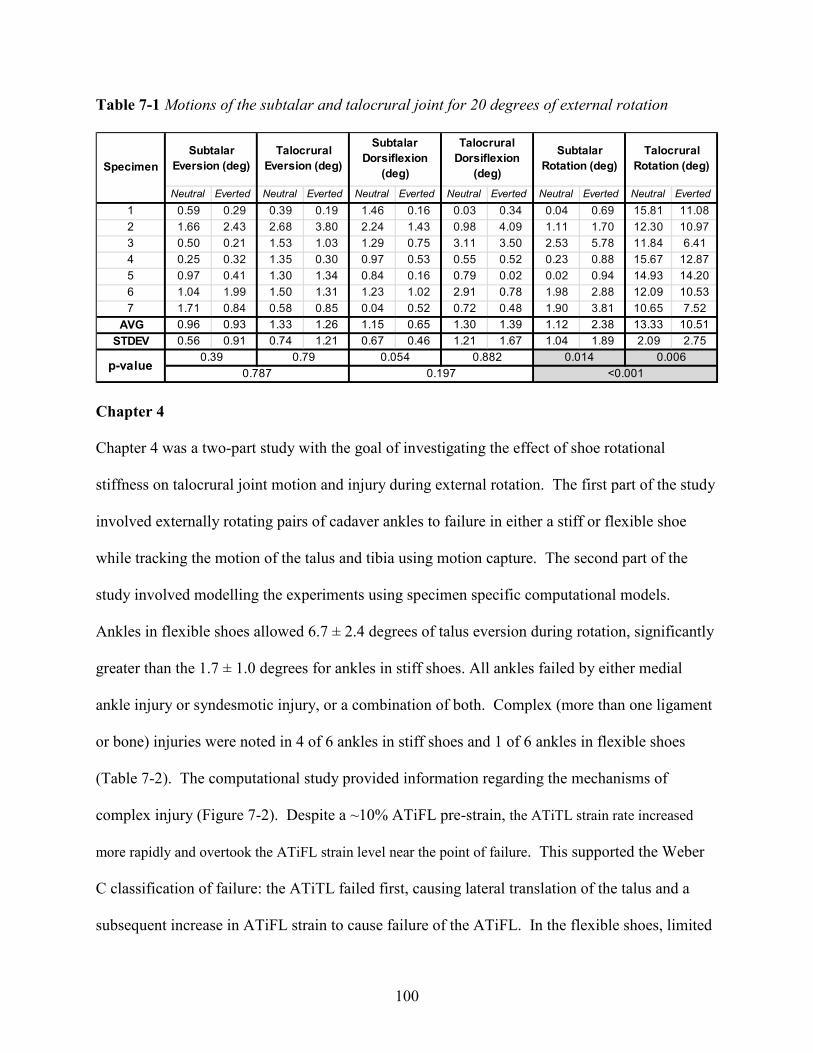
100

Table 7-1 Motions of the subtalar and talocrural joint for 20 degrees of external rotation

Chapter 4

Chapter 4 was a two-part study with the goal of investigating the effect of shoe rotational

stiffness on talocrural joint motion and injury during external rotation. The first part of the study

involved externally rotating pairs of cadaver ankles to failure in either a stiff or flexible shoe

while tracking the motion of the talus and tibia using motion capture. The second part of the

study involved modelling the experiments using specimen specific computational models.

Ankles in flexible shoes allowed 6.7 ± 2.4 degrees of talus eversion during rotation, significantly

greater than the 1.7 ± 1.0 degrees for ankles in stiff shoes. All ankles failed by either medial

ankle injury or syndesmotic injury, or a combination of both. Complex (more than one ligament

or bone) injuries were noted in 4 of 6 ankles in stiff shoes and 1 of 6 ankles in flexible shoes

(Table 7-2). The computational study provided information regarding the mechanisms of

complex injury (Figure 7-2). Despite a ~10% ATiFL pre-strain, the ATiTL strain rate increased

more rapidly and overtook the ATiFL strain level near the point of failure. This supported the Weber

C classification of failure: the ATiTL failed first, causing lateral translation of the talus and a

subsequent increase in ATiFL strain to cause failure of the ATiFL. In the flexible shoes, limited

Neutral Everted Neutral Everted Neutral Everted Neutral Everted Neutral Everted Neutral Everted

0.59 0.29 0.39 0.19 1.46 0.16 0.03 0.34 0.04 0.69 15.81 11.08

1.66 2.43 2.68 3.80 2.24 1.43 0.98 4.09 1.11 1.70 12.30 10.97

0.50 0.21 1.53 1.03 1.29 0.75 3.11 3.50 2.53 5.78 11.84 6.41

0.25 0.32 1.35 0.30 0.97 0.53 0.55 0.52 0.23 0.88 15.67 12.87

0.97 0.41 1.30 1.34 0.84 0.16 0.79 0.02 0.02 0.94 14.93 14.20

1.04 1.99 1.50 1.31 1.23 1.02 2.91 0.78 1.98 2.88 12.09 10.53

1.71 0.84 0.58 0.85 0.04 0.52 0.72 0.48 1.90 3.81 10.65 7.52

0.96 0.93 1.33 1.26 1.15 0.65 1.30 1.39 1.12 2.38 13.33 10.51

0.56 0.91 0.74 1.21 0.67 0.46 1.21 1.67 1.04 1.89 2.09 2.75

Talocrural

Dorsiflexion

(deg)

Subtalar

Rotation (deg)

Talocrural

Rotation (deg)

1

2

3

4

5

Specimen

Subtalar

Eversion (deg)

Talocrural

Eversion (deg)

Subtalar

Dorsiflexion

(deg)

6

7

AVG

STDEV

p-value0.39 0.79 0.054 0.882 0.014 0.006

0.787 0.197 <0.001

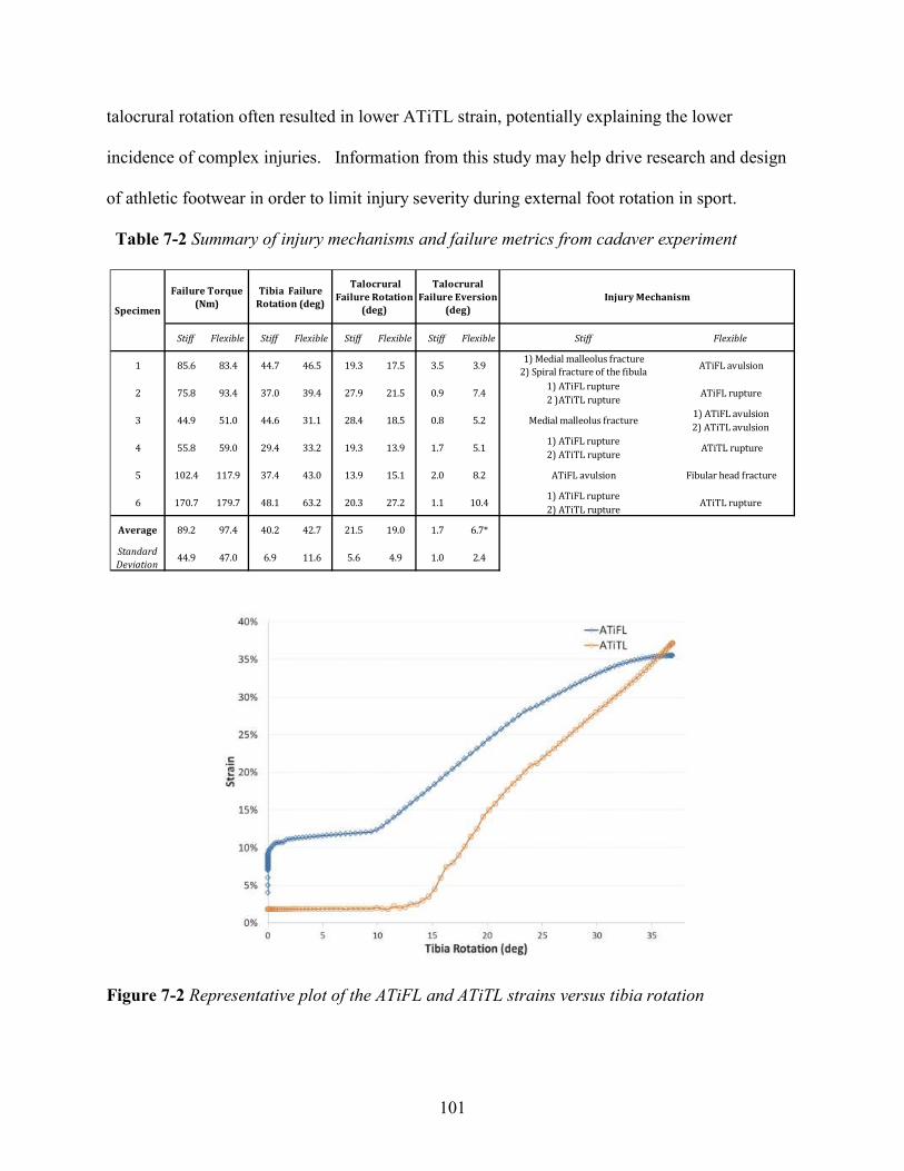
101

talocrural rotation often resulted in lower ATiTL strain, potentially explaining the lower

incidence of complex injuries. Information from this study may help drive research and design

of athletic footwear in order to limit injury severity during external foot rotation in sport.

Table 7-2 Summary of injury mechanisms and failure metrics from cadaver experiment

Figure 7-2 Representative plot of the ATiFL and ATiTL strains versus tibia rotation

Stiff Flexible Stiff Flexible Stiff Flexible Stiff Flexible

1 85.6 83.4 44.7 46.5 19.3 17.5 3.5 3.9

5 102.4 117.9 37.4 43.0 13.9 15.1 2.0 8.2

Average 89.2 97.4 40.2 42.7 21.5 19.0 1.7 6.7*

Standard

Deviation44.9 47.0 6.9 11.6 5.6 4.9 1.0 2.4

5.20.818.5

Injury Mechanism

ATiFL rupture

Talocrural

Failure Eversion

(deg)

0.9 7.475.8

Stiff Flexible

Specimen

Talocrural

Failure Rotation

(deg)

Tibia Failure

Rotation (deg)

Failure Torque

(Nm)

2) ATiTL avulsion

1) ATiFL rupture

2 )ATiTL rupture

1) Medial malleolus fracture

2) Spiral fracture of the fibulaATiFL avulsion

ATiFL avulsion Fibular head fracture

ATiTL rupture1) ATiFL rupture

2) ATiTL rupture

Medial malleolus fracture1) ATiFL avulsion

61) ATiFL rupture

2) ATiTL ruptureATiTL rupture10.41.127.220.363.2

13.9

28.4

19.3

31.1

33.2 5.11.729.459.055.8

39.4 27.9 21.537.093.4

48.1

44.651.044.9

2

3

4

179.7170.7

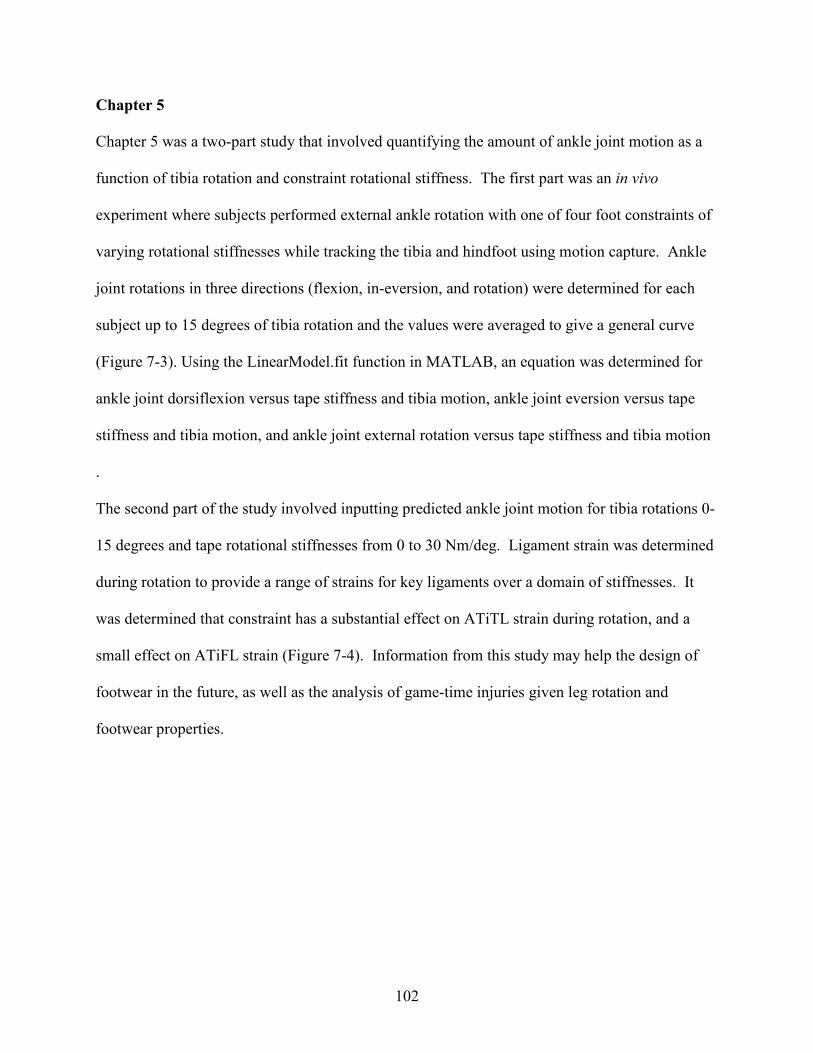
102

Chapter 5

Chapter 5 was a two-part study that involved quantifying the amount of ankle joint motion as a

function of tibia rotation and constraint rotational stiffness. The first part was an in vivo

experiment where subjects performed external ankle rotation with one of four foot constraints of

varying rotational stiffnesses while tracking the tibia and hindfoot using motion capture. Ankle

joint rotations in three directions (flexion, in-eversion, and rotation) were determined for each

subject up to 15 degrees of tibia rotation and the values were averaged to give a general curve

(Figure 7-3). Using the LinearModel.fit function in MATLAB, an equation was determined for

ankle joint dorsiflexion versus tape stiffness and tibia motion, ankle joint eversion versus tape

stiffness and tibia motion, and ankle joint external rotation versus tape stiffness and tibia motion

.

The second part of the study involved inputting predicted ankle joint motion for tibia rotations 0-

15 degrees and tape rotational stiffnesses from 0 to 30 Nm/deg. Ligament strain was determined

during rotation to provide a range of strains for key ligaments over a domain of stiffnesses. It

was determined that constraint has a substantial effect on ATiTL strain during rotation, and a

small effect on ATiFL strain (Figure 7-4). Information from this study may help the design of

footwear in the future, as well as the analysis of game-time injuries given leg rotation and

footwear properties.

103

Figure 7-3 Mean ankle joint dorsiflexion, external rotation, and eversion vs. tibia rotation for

three tapes and a tapeless condition.

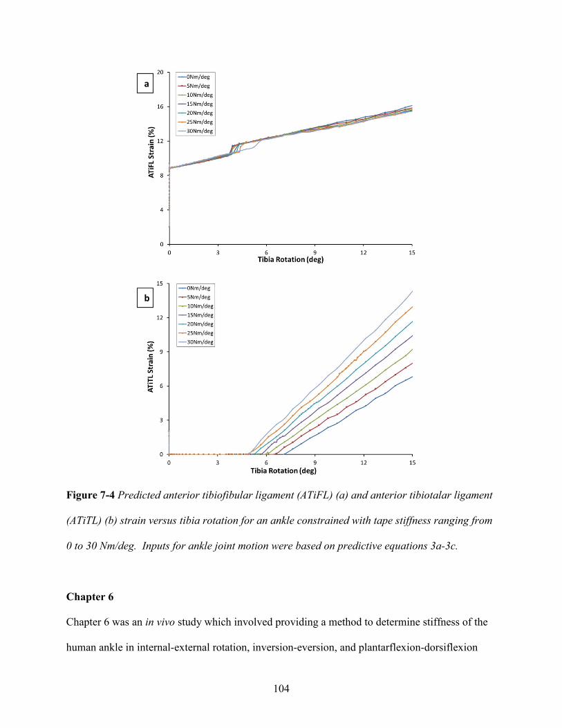
104



0 to 30 Nm/deg. Inputs for ankle joint motion were based on predictive equations 3a-3c.

Chapter 6

Chapter 6 was an in vivo study which involved providing a method to determine stiffness of the

human ankle in internal-external rotation, inversion-eversion, and plantarflexion-dorsiflexion

a

b

105

during a single-legged external foot rotation experiment. Five male subjects stood on one foot

and performed an internal rotation of the body (external rotation of the foot) on a force plate,

while motions were captured with a motion capture system. Hindfoot rotations relative to the

tibia and resistive moments in the above three directions were obtained using a commercial

software package. The resistive moments were plotted against rotation during the loading

portions of the curves. Linear approximations of these curves were used to determine stiffness of

the ankle in directions of internal-external, inversion-eversion, and plantarflexion-dorsiflexion.

This method can be used in the future for a variety of athletic motions in order to more fully

characterize human ankle stiffness under different loading situations on the athletic field. The

data can then be useful for the development of surrogate test devices to evaluate athletic

performance and ankle injury risk characteristics of shoe-surface interfaces.

Table 7-3 Ankle stiffness in three directions obtained from subjects performing a single legged

external rotation of the foot.

1 2 3 4 5

52.47 (23.63) 75.20 (19.07) 61.83 (15.65) 43.00 (11.49) 86.21 (16.51) 63.75 17.3

0.93 0.04R2 0.89 (0.14) 0.89 (0.08) 0.99 (0.01) 0.92 (0.04) 0.97 (0.04)

4.31

Range (deg) 0.72 (0.35) 4.54 (1.28) 3.27 (0.23) 2.77 (2.21) 2.11 (0.95) 2.68 1.41

0.97 0.02

Plantarflexion/dorsiflexion

Stiffness (Nm/deg) 12.13 (0.08) 3.47 (1.13) 8.05 (1.60) 2.20 (0.53) 2.50 (1.07) 5.68

R2 0.99 (0.00) 0.96 (0.05) 0.95 (0.05) 0.98† 0.98 (0.01)

0.72

Range (deg) 6.72 (3.78) 2.77 (1.56) 1.03 (0.50) 4.14† 1.37 (0.43) 3.2 2.32

0.99 0.01

Inversion/eversion

Stiffness (Nm/deg) 0.71 (0.35) 1.67 (1.05) 2.13 (0.92) 2.08† 2.64 (.28) 1.85

R2 0.98 (0.00) 0.99 (0.01) 0.99 (0.00) 0.98 (0.02) 0.99 (0.00)

2.19 0.52

Range (deg) 11.87 (6.69) 18.41 (5.78) 14.69 (4.98) 5.93 (1.00) 23.69 (4.84) 14.92 6.69

Mean SD

Rotation Speed (deg/s)

Internal/external rotation

Stiffness (Nm/deg) 1.80 (0.86) 1.52 (0.23) 2.67 (1.03) 2.65 (0.65) 2.31 (0.04)

Subject

106

Contributions to the Literature

This dissertation has made three major contributions to the current literature:

Influence of shoe design on ankle movement and injury

Previous studies have investigated shoe-surface interaction as an indicator of rotational injury

risk, but few studies have studied the effect of a shoe’s rotational stiffness on injury. A primary

contribution of this dissertation was the investigation of the effect shoe rotational stiffness has on

ankle joint motion, ligament strain, and injury generated. This was first looked at in Chapter 4,

which showed that shoe rotational stiffness not only affected the amount of talocrural joint

eversion and rotation during external foot rotation, but also the severity of injury generated and

distribution of ligament strains. It was concluded that stiff shoes limit talocrural joint eversion

during ankle external rotation, but maximize talocrural joint rotation. This resulted in high

anterior deltoid strains and complex injuries. The interaction between rotational stiffness and

talocrural joint motion was quantified in Chapter 5. The equations presented in this chapter will

enable future researchers to more accurately assess ankle joint motion given gross foot rotation

and shoe rotational stiffness. Additionally, this may aid in the design of footwear with the goal

of limiting time-loss due to severe ankle injury.

Determination of failure-level ligament strains

While previous studies have performed mechanical testing on ex vivo ligaments in order to

determine failure properties, little information exists regarding the amount of strain ligaments

undergo at failure in situ. A second major contribution of this dissertation was the correlation of

ligament strain level with severity of damage. This was accomplished first in Chapter 2, which

107

involved using specimen-specific computational models to simulate failure-level cadaver studies.

The strain magnitudes in grade II vs. grade III sprains were compared and were determined to be

significantly different (25.5 ± 4.2% vs. 31.8 ± 3.8%, respectively). This was verified in Chapter

4, in which simulations modelling complete ruptures showed ligament failure at 29.1 ± 6.7%.

These magnitudes could be used to assess potential injury risk (such as in Chapter 6), in order to

design shoes, or determine the effect of different loading conditions on injury likelihood.

Use of specimen-specific computational models

While a generic model provides useful information regarding relationships between motion and

injury mechanisms, it is believed that specimen-specific modeling provides more exact strain

information. A third contribution of this dissertation to the literature was the use of specimen-

specific computational modelling to analyze ankle kinematics and injury. The curvature of the

tronchlea tali (top surface of the talus) determines the stability of the ankle in the anterior

posterior direction and the talar facets (contacting surfaces) have a significant impact on the

position of the axis of movements between the talus and calcaneus. The differences in ankle

mechanics can significantly affect injury risk as talar motion plays a significant role in both

medial and high ankle sprains. The use of specimen-specific ankle modeling can be expanded to

investigate in vivo injuries by looking at scenarios where the geometry and motion of a subject

are known. By looking at these scenarios, the specifics of the injury can be analyzed, thus aiding

in the design of intervention strategies and equipment to limit the severity and frequency of

athletic ankle injuries.

108

APPENDICES

109

APPENDIX 1: RESEARCH PUBLICATIONS

Peer Reviewed Manuscripts

1. Dutcheshen N, Maerz T, Rabban P, Haut RC, Button KD, Baker KC, Guettler J. (2012) The

acute effect of bipolar radiofrequency energy thermal chondroplasty on intrinsic biomechanical

properties and thickness of chondromalacic human articular cartilage. Journal of Biomechanical

Engineering. 134(8):081007.

2. Meyer EG, Wei F, Button KD, Haut RC. (2012) Determination of ankle ligament strain using

a rigid body computational model for sports injury scenarios. Proceedings-International Research

Council on the Biomechanics of Injury. 277-288.

3. Button KD, Wei F, Meyer EG, Haut RC. (2012) Specimen-specific computational models of

ankle sprains produced in a laboratory setting. Journal of Biomechanical Engineering. 135(4),

041001.

4. Button KD, Braman JE, Wei F, Haut RC. (2013) A method of determining in vivo dynamic

human ankle stiffness under external foot rotation. Journal of Sports Engineering and

Technology. 228(2), 120-124.

5. Fischenich KM, Button KD, Decamp CD, Haut RC, Donahue TL. (2014) Evaluation of

meniscal mechanics and proteoglycan content in a modified ACL transection model for

osteoarthritis. Journal of Biomechanical Engineering. 136(7), 071001. *Editors' Choice Paper

for 2014*

6. Fischenich KM, Button KD, Coatney GA, Fajardo RS, Leikert KM, Haut RC, Donahue TL.

(2014) Chronic changes in the articular cartilage and meniscus following traumatic impact to the

lapine knee. Journal of Biomechanics. doi:10.1016/j.jbiomech.2014.11.038

7. Wheatley BB, Fischenich KM, Button KD, Haut RC, Haut Donahue TL. (2015) An

optimized transversely isotropic, hyper-poro-viscoelastic finite element model of the meniscus to

evaluate mechanical degradation. Journal of Biomechanics. (In Press).

8. Button KD, Braman JE, Davison MA, Wei F, Schaeffer MC, Haut RC. (2014) Rotational

stiffness of American football shoes affects ankle biomechanics and injury severity. Journal of

Biomechanical Engineering. doi: 10.1115/1.4029979

9. Coatney GA, Abraham AC, Fischenich KM, Button KD, Haut RC, Haut Donahue TL. (2014)

Efficacy of P188 on lapine meniscus preservation following blunt trauma. Journal of the

Mechanical Behavior of Biomedical Materials. (In Publication).

10. Button KD, Braman JE, Davison MA, Wei F, Haut RC. (2014) Effect of pre-eversion on

talocrural and subtalar joint motion during ankle external rotation. Journal of Biomechanics. (In

Revision).

110

11. Pauly HM, Larson BE, Coatney GA, Button KD, DeCamp CE, Fajardo RS, Haut RC, Haut

Donahue TL. (2015) Assessment of cortical and trabecular bone changes in two models of post-

traumatic osteoarthritis. Journal of Orthopaedic Research (In Revision).

12. Fischenich KM, Button KD, Fajardo RS, DeCamp CE, Haut RC, Haut Donahue TL. (2015)

Tissue changes in surgical and traumatically-induced experimental models of knee joint injury

using magnetic resonance imaging. Magnetic Resonance Imaging (In Review).

13. Button KD, Thornton PA, Braman JE, Wei F, Haut RC. (2015) Determining ankle joint

motion and ligament strain during ankle rotation for a given rotational stiffness constraint.

Journal of Sports Engineering and Technology (In Review)

Peer Reviewed Abstracts

1. Button KD, Braman JE, Wei F, Haut RC. (2012) Determination of in vivo dynamic human

ankle stiffness under external foot rotation. ASME Summer Bioengineering Conf. Fajardo,

Puerto Rico. SBC2012-80373.

2. Button KD, Wei F, Meyer EG, Fitzsimons K, Haut RC. (2012) Determination of in situ ankle

ligament strains in cases of high and medial ankle sprains. ASME Summer Bioengineering Conf.

Fajardo, Puerto Rico. SBC2012-80378.

3. Pauly HM, Larson BE, Button KD, Haut RC, Donahue TL. (2013) Micro-Computed

tomography analysis of bone volume following traumatic closed joint injury. Rocky Mountain

American Society of Biomechanics Meeting, April, 2013, Estes Park, CO.

4. Coatney GA, Abraham AC, Button KD, Haut RC, Donahue TL. (2013) P188 efficacy on

lapine meniscus preservation following blunt trauma. Rocky Mountain American Society of

Biomechanics Meeting, April, 2013, Estes Park, CO.

5. Fischenich KM, Button KD, Fajardo RS, Decamp CD, Haut RC, Donahue TL. (2013)

Mechanical evaluation of menisci following surgical transection of both menisci and anterior

cruciate ligament. Rocky Mountain American Society of Biomechanics Meeting, April, 2013,

Estes Park, CO.

6. Fischenich KM, Button KD, Fajardo RS, Haut RC, Donahue TL. (2013) Evaluation of

menisci following a traumatic compressive tibiofemoral load. ASME Summer Bioengineering

Conf. Sunriver, Oregon. SBC2013-14193.

7. Button KD, Leikert K, Donahue TL, Haut RC. (2013) Development of a traumatic anterior

cruciate ligament and meniscal rupture model to study osteoarthritis. ASME Summer

Bioengineering Conf. Sunriver, Oregon. SBC2013-14287.

111

8. Button KD, Davison M, Braman JE, Schaefer MC, Haut RC. (2013) Effect of shoe stiffness

on injury produced under external rotation of the foot in human cadavers. ASME Summer

Bioengineering Conf. Sunriver, Oregon, 2013. SBC2013-14719.

9. Fischenich KM, Coatney GA, Haverkamp J, Button KD, DeCamp C, Haut RC, Haut

Donahue TL. (2013) Meniscal glycosaminoglycan coverage twelve weeks post injury in two

models of knee joint injury. 11th World Congress of the International Cartilage Repair Society,

Sept. 15-18, 2013, Izmir, Turkey.

10. Button KD, Steibel JP, Karcher DM, Haut RC. (2014) A non-invasive method to predict

laying hen bone mechanical properties. Poultry Science Association Annual Meeting. Christi,

Texas. PSA-161.

11. Button KD, Davison M, Braman JE, Schaefer MC, Haut RC. (2014) Investigating the effects

of shoe stiffness on ankle injury risk using computational models. 7th World Congress in

Biomechanics. Boston, MA. 14-IS-2161-WCB.

12. Button KD, Leikert KM, DeCamp CD, Donahue TL, Haut RC. (2014) Comparison of a

traumatic ACL rupture and modified transection model to study osteoarthritis. 7th World

Congress in Biomechanics. Boston, MA. 14-A-1633-WCB.

13. Donahue TL, Fischenich KM, Coatney G, Pauly H, Button KD, Haut RC. (2014) Two new

experimental models of post-traumatic knee joint injury. 7th World Congress in Biomechanics.

Boston, MA. 14-IS-2706-WCB.

14. Fischenich KM, Button KD, Fajardo RS, Decamp CD, Haut RC, Donahue TL. (2014) A

longitudinal comparison of mechanical changes of the menisci in two models of posttraumatic

osteoarthritis of the knee. 7th World Congress in Biomechanics. Boston, MA. 14-A-1696-WCB.

15. Pauly HM, Larson BE, Button KD, DeCamp CD, Haut RC, Donahue TL. (2014) Micro-

computed tomography comparison of trabecular bone changes in rabbits following surgical

transection of anterior cruciate ligament and menisci or traumatic impact to the tibiofemoral

joint. 60th Annual Meeting of the Orthopaedic Research Society. March 15-18, 2014. New

Orleans, LA.

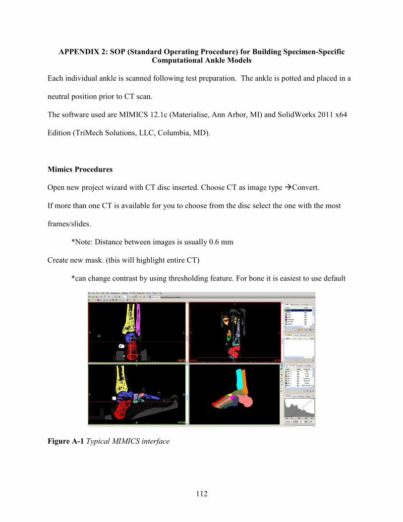
112

APPENDIX 2: SOP (Standard Operating Procedure) for Building Specimen-Specific Computational Ankle Models

Each individual ankle is scanned following test preparation. The ankle is potted and placed in a

neutral position prior to CT scan.

The software used are MIMICS 12.1c (Materialise, Ann Arbor, MI) and SolidWorks 2011 x64

Edition (TriMech Solutions, LLC, Columbia, MD).

Mimics Procedures

Open new project wizard with CT disc inserted. Choose CT as image type �Convert.

If more than one CT is available for you to choose from the disc select the one with the most

frames/slides.

*Note: Distance between images is usually 0.6 mm

Create new mask. (this will highlight entire CT)

*can change contrast by using thresholding feature. For bone it is easiest to use default

Figure A-1 Typical MIMICS interface

113

Select Region Growing. Use cursor to select highlighted area of bone of interest in one of the 3

CT scan viewing windows. This will create a new mask; rename it for the current bone. Deselect

the original mask.

Use the edit mask in 3D feature to check that only the bone of interest is selected under the new

mask.

If there is more than one bone selected go through the CT scan frame by frame and outline the

bone of interest with eraser using edit masks feature. This will give you a large enough gap

between bone of interest and excess area to use the edit mask in 3D feature to erase remaining

excess bone.

*use Edit in 3D cautiously, it will erase anything in the plane behind the cursor

*also you can change size and shape of the erasing cursor using the options at the

bottom of the screen or in its toolbar

When excess mask is removed choose Calculate 3D and select the mask that was just cleaned up.

For quality choose high. A 3D model will appear in the lower right screen.

Right click the 3D model just created in the side bar and choose surface wrap. (For larger bones

use 4 mm for both settings, for smaller use 3 mm to 2.5 mm for both settings.)

Right click the surface wrapped model and choose calculate Mask from 3D. This will generate a

new mask which you must check for overlap with other bones in the CT scan and for hollow

spaces in the center. When this mask is sufficient, repeat step 7. You may delete all masks and

3D models except for the final mask and final model created.

Again right click the 3-D model and choose smoothing. Use a smoothing factor of 0.9 for all

bones. The Number of iterations varies, and is somewhat at your discretion for how much

important detail should be kept. Make sure that keep originals is unchecked and compensate

114

shrinkage is checked. (# of iterations used for tibia and fibula was 4, calcaneus and talus was 2,

navicular, cuneiforms and metatarsals was 1, no smoothing was done on the phalanges)

Repeat steps 4 thru 10 for all bones of interest. (Hint: it may be helpful to use the Boolean

operator after finishing each bone to delete the mask created from the general mask that you start

your region growing from)

After all bones are completed, Go to FEA/CFD>>remesh>>select all

For smoothing (1st) and remeshing (2nd) use the following settings

Fixing>>Smooth

Method: Laplacian (1st order)

Smooth Factor: 0.9

Number of Iterations: 5

Remeshing>>Auto Remesh

Shape Quality Threshold: 0.3

Max Geometrical Error: 0.5

Number of Iterations: 3

Goto File>>Export>>Binary STL file and select appropriate folder for solidworks files. (File size

should be 100KB or less, If files are too large consider reprocessing with less detail)

115

Solid Works Processing

To open files in Solid works, you must go to open, and choose file type of mesh files. Select the

STL that was exported from MIMICS

Goto Tool>>ScanTo3D>>Mesh Prep Wizard>>select bone file

Continue to hit the next arrow in the dialog box that appears until you get to global

simplification. Here choose reduction amount of 50% unless the number of surfaces is already

less than 200.

Choose no smoothing in the next dialog box and when the option is available check the box to

launch the surface wizard.

Use surface wizard to create 3D object select Automatic creation from the radial buttons in the

first window.

Under surface detail select Update Preview. Check the number of surfaces and surface errors.

If more than one surface error occurs, choose the red x in the upper left corner of the surface

wizard. Go back to mesh prep wizard and change global smoothing by moving the slider bar one

tick mark to the right. Repeat steps with surface wizard.

If there is still more than one error go back to mesh prep wizard and reduce by 10%. Repeat until

there are only one or two surface errors.

With only one or two surface errors move slider bar to increase surface detail and update the

preview again. Continue to move slider to the right and update until error is gone.

Check the number of surfaces. If over 300 continue same reduction and smoothing process as

was used for multiple errors in the preview.

If there are no errors and there are less than 300 surfaces choose the green checkmark to finish

the bone and save in a new folder of revised files.

116

Repeat process with all bones exported form MIMICS.

*Hint: for best luck with spring placement in assembly be sure that calcaneus and talus

have at least 150 surfaces, closer to 300 would be better because of the number of springs that

are placed on these bones.

SolidWorks Assembly and Motion Analysis

Choose new SolidWorks document type assembly.

Insert Components>>Choose tibia first as fixed part of the assembly.

Order of insertion for remaining components doesn’t matter. Mate components origin and align

axes to adjacent bones in order to place them in correct 3D space

Go to motion study tab; in drop down menu choose study type: Motion Analysis.

For new spring, choose the spring icon. Make it a linear spring and choose two insertion nodes

based on insertions of previous models and references. (Atlas of Human Anatomy works well)

Choose stiffness based on literature and previous models. To pre-strain the springs, take the

original free length shown in the spring tool box and divide by 1.02 to get 2% strain. Copy this

value back into the spring toolbox and check the box to update to model changes.

Add 3D surface contacts by selecting two adjacent bones and clicking on the ‘3D surface

contacts’.

Uncheck the ‘material’ and ‘friction’ box. This will allow your model to run much quicker.

Under ‘Elastic Properties’, set:

Stiffness: 10000 N/mm

Exponent: 1.75

Max. Damping: 50 N/(mm/s)

117

Penetration: 0.001 mm

If there is still overlap after running a model, decrease the penetration or increase stiffness and

run again.

Before running either motor or motion data for calculation, check that the fibula, calcaneus, and

talus are not mated and are free to move.

To create more than one simulation with same model, right click motion study tab and

‘Duplicate’, this will save time in placing a springs in a new motion study.

Under study properties, lower the accuracy and the number of frames persecond. (Frames per

second can be lowered to as little as 5 per second). Check the box to show all motion analysis

messages—this will be helpful in troubleshooting the simulation.

Under the advanced options, the integrator can be either gstiff or wstiff and the initial integrator

step size can be lowered to if an error occurs during calculation.

Close all other programs on the computer and select the calculate icon. Running background

programs will slow the calculation and sometimes cause the program to get hung up for hours.

Torques, displacements, velocities and other motion data can be retrieved after the simulation is

finished by opening the plots toolbox.

In order to calculate strain values, click on the ‘Results’ icon and select a spring. Select

‘Displacement/Velocity/Acceleration>>Linear Displacement>>Magnitude’. Right click on the

plot and select ‘Export to Spreadsheet’. This will give you the length of the spring over time.

To calculate strain, copy the length values into ‘Ligament_Strain_Template.xls’ in the SOP

folder. Enter the original ligament length. Repeat this step for all ligaments of interest.

118

APPENDIX 3: SOP (Standard Operating Procedure) For Calculating Ankle Joint Motion Given Vicon Data

This document will outline how to calculate the amount of talocrural joint inversion/eversion,

plantarflexion/dorsiflexion, and internal/external rotation given a three dimensional, orthogonal

axis on each bone (Figure A-2). The same procedure can be followed for the subtalar joint

The raw motions can come from either cadaver data (where the marker arrays are screwed into

the bone) (Figure A-3a) or in vivo data (where the markers are taped to the skin) (Figure A-3b)

Figure A-2 Orthogonal coordinate axes on the tibia, talus, and calcaneus.

119

Figure A-3 Marker arrays in a cadaver ankle (a) and human subject (b)

a

b

120

Mathematical Background

Since the arrays are randomly oriented, transformations need to be performed to align the local x,

y, and z axes with the global Cartesian coordinate system. For the talus:

A= > ? ?? > ?? ? >

B=Initial orientation of talus in local coordinates

C=Final position of talus in local coordinates

R1=

@A ∙ BA @A ∙ BC @A ∙ BD@C ∙ BA @C ∙ BC @C ∙ BD@D ∙ BA @D ∙ BC @D ∙ BC

R2=

EA ∙ BA EA ∙ BC EA ∙ BDEC ∙ BA EC ∙ BC EC ∙ BDED ∙ BA ED ∙ BC ED ∙ BC

R3=R1TR2

R4=R3T

C’= R4A (Final orientation of talus in global coordinates)

Establish Joint Coordinate System based on final positions of arrays. For talocrural (C’=final

talus, D’=final tibia):

�� = F′�

� = E′

�� =�� ×��

|�� ×��|

� = �� ∙ F′� (flexion)

� = �� ∙ E′�� (rotation)

� = �� ∙ �� (inversion/eversion)

121

Procedure

Open up ‘JCS.m’ in ‘Z:\bimgrad\SOP\JCS ANALYSIS’

The program is written for a right ankle oriented with the foot on the ground. If the foot is

upside down, or the analysis is run for a left ankle, adjustments will need to be made to the signs

of alpha, gamma, and beta in lines 80-82 and 91-93.

Line 9: type the location of your Vicon data

Line 10: specify where you want the output data to go (note: this file must be closed when

running the program)

Line 105: specify what sheet you want to write the data to (term 3) and what range within the

sheet (term 4).

Run the program by hitting the green arrow in the task bar.

The program will give 6 columns of data. The columns should be labelled accordingly:

The program is shown below.

Tibia External

Rotation

Relative to

Global

Talus

Dorsiflexion

Relative to Tibia

Talus External

Rotation

Relative to Tibia

Talus Eversion

Relative to Tibia

Tibia

Dorsiflexion

Relative to

Global

Tibia Eversion

Relative to

Global

122

%************************************************** ************************ %written by Keith D. Button %************************************************** ************************ %file to calculate talocrural dorsiflexion, externa l rotation, and eversion %for a right ankle. For a left ankle, multiply lin es 76 and 77 by -1. %************************************************** ************************ clear, clc %************************************************** ************************ file= '(Vicon data file name and location)' ; %Input Vicon data file location out= '(Output file location)’ ; %specify output file location M=xlsread(file,1, 'AG1:BD10000' ); %data range in file for both tibia and talus positi ons (should be 24 columns) sizem=size(M); r=sizem(1); %number of data points in file Result=zeros(r,6); tibia1=M(1,1:12); %initial talus position talus1=M(1,13:24); %initial tibia position %************************************************** ************************ origin=[0 0 0 1 0 0 0 1 0 0 0 1]; Axraw= [origin(4)-origin(1),origin(5)-origin(2),ori gin(6)-origin(3)]; Ax=Axraw/norm(Axraw); Ayraw= [origin(7)-origin(1),origin(8)-origin(2),ori gin(9)-origin(3)]; Ay=Ayraw/norm(Ayraw); Azraw= [origin(10)-origin(1),origin(11)-origin(2),o rigin(12)-origin(3)]; Az=Azraw/norm(Azraw); A=[Ax; Ay; Az]; %matrix for orthogonal neutral axis %************************************************** ************************ i=1; for i=1:r tibia2=M(i,1:12); %talus position talus2=M(i,13:24); %tibia position Bxraw= [talus1(4)-talus1(1),talus1(5)-talus1(2) ,talus1(6)-talus1(3)]; Bx=Bxraw/norm(Bxraw); Byraw= [talus1(7)-talus1(1),talus1(8)-talus1(2) ,talus1(9)-talus1(3)]; By=Byraw/norm(Byraw); Bzraw= [talus1(10)-talus1(1),talus1(11)-talus1( 2),talus1(12)-talus1(3)]; Bz=Bzraw/norm(Bzraw); B=[Bx; By; Bz]; %talus initial position in local coordinates Cxraw= [talus2(4)-talus2(1),talus2(5)-talus2(2) ,talus2(6)-talus2(3)]; Cx=Cxraw/norm(Cxraw); Cyraw= [talus2(7)-talus2(1),talus2(8)-talus2(2) ,talus2(9)-talus2(3)]; Cy=Cyraw/norm(Cyraw); Czraw= [talus2(10)-talus2(1),talus2(11)-talus2( 2),talus2(12)-talus2(3)]; Cz=Czraw/norm(Czraw); C=[Cx ; Cy; Cz]; %talus position after external rotation in local co ordinates %************************************************** ************************ Dxraw= [tibia1(4)-tibia1(1),tibia1(5)-tibia1(2) ,tibia1(6)-tibia1(3)]; Dx=Dxraw/norm(Dxraw); Dyraw= [tibia1(7)-tibia1(1),tibia1(8)-tibia1(2) ,tibia1(9)-tibia1(3)]; Dy=Dyraw/norm(Dyraw); Dzraw= [tibia1(10)-tibia1(1),tibia1(11)-tibia1( 2),tibia1(12)-tibia1(3)]; Dz=Dzraw/norm(Dzraw); D=[Dx; Dy; Dz]; %tibia initial position in local coordinates Exraw= [tibia2(4)-tibia2(1),tibia2(5)-tibia2(2) ,tibia2(6)-tibia2(3)]; Ex=Exraw/norm(Exraw); Eyraw= [tibia2(7)-tibia2(1),tibia2(8)-tibia2(2) ,tibia2(9)-tibia2(3)]; Ey=Eyraw/norm(Eyraw); Ezraw= [tibia2(10)-tibia2(1),tibia2(11)-tibia2( 2),tibia2(12)-tibia2(3)]; Ez=Ezraw/norm(Ezraw); E=[Ex ; Ey; Ez]; %tibia position after external rotation in local co ordinates %************************************************** ************************ ROT21=[dot(Bx,Ax),dot(Bx,Ay),dot(Bx,Az);dot(By,Ax), dot(By,Ay),dot(By,Az);dot(Bz,Ax),dot(Bz,Ay),dot(Bz,Az)]; ROT22=[dot(Cx,Ax),dot(Cx,Ay),dot(Cx,Az);dot(Cy,Ax), dot(Cy,Ay),dot(Cy,Az);dot(Cz,Ax),dot(Cz,Ay),dot(Cz,Az)]; ROT23=ROT22*transpose(ROT21); ROT24=transpose(ROT21)*ROT22; ROT25=transpose(ROT24); C2=ROT25*A; %talus final position along anatomical axis

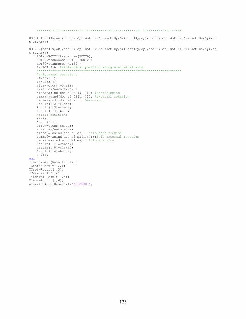
123

%************************************************** ************************ ROT26=[dot(Dx,Ax),dot(Dx,Ay),dot(Dx,Az);dot(Dy,Ax), dot(Dy,Ay),dot(Dy,Az);dot(Dz,Ax),dot(Dz,Ay),dot(Dz,Az)]; ROT27=[dot(Ex,Ax),dot(Ex,Ay),dot(Ex,Az);dot(Ey,Ax), dot(Ey,Ay),dot(Ey,Az);dot(Ez,Ax),dot(Ez,Ay),dot(Ez,Az)]; ROT28=ROT27*transpose(ROT26); ROT29=transpose(ROT26)*ROT27; ROT30=transpose(ROT29); E2=ROT30*A; %tibia final position along anatomical axis %************************************************** ************************ %talocrural rotations e1=E2(1,:); e3=C2(3,:); e2raw=cross(e3,e1); e2=e2raw/norm(e2raw); alpha=asind(dot(e2,E2(3,:))); %dorsiflexion gamma=asind(dot(e2,C2(1,:))); %external rotation beta=asind(-dot(e1,e3)); %eversion Result(i,2)=alpha; Result(i,3)=gamma; Result(i,4)=beta; %tibia rotations e4=Ax; e6=E2(3,:); e5raw=cross(e6,e4); e5=e5raw/norm(e5raw); alpha2=-asind(dot(e5,Az)); %tib dorsiflexion gamma2=-asind(dot(e5,E2(1,:))); %tib external rotation beta2=-asind(-dot(e4,e6)); %tib eversion Result(i,1)=gamma2; Result(i,5)=alpha2; Result(i,6)=beta2; i=i+1; end Tibrot=real(Result(:,1)); TCdors=Result(:,2); TCrot=Result(:,3); TCev=Result(:,4); Tibdorsi=Result(:,5); Tibev=Result(:,6); xlswrite(out,Result,1, 'A2:F500' );

124

Table A-1: Raw Data from Cadaver Failure Tests (Chapter 4)

1477 Left 1477 Right

Failure Point Failure Point

Torque (Nm) Rotation (deg) Torque (Nm) Rotation (deg)

85.55 44.69 83.39 46.48

Incremental Incremental

4.04 5.03 5.47 5.05

11.46 10.03 13.85 10.12

18.66 15.13 22.75 15.15

26.56 20.02 32.63 20.14

36.06 25.06 43.07 25.12

46.19 30.10 54.88 30.16

57.04 35.02 66.50 35.14

68.63 40.11 76.56 40.03

77.68 45.06 79.56 45.02




75.80 37.02 93.35 39.42


6.36 5.06 8.33 5.07

15.62 10.06 17.82 10.05

26.47 15.06 29.44 15.08

38.99 20.04 43.13 20.10

52.47 25.13 57.66 25.10

65.89 30.05 72.82 30.03

73.81 35.08 85.30 35.05

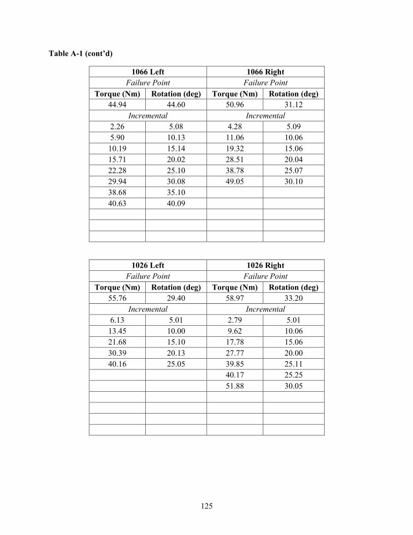
125

Table A-1 (cont’d)




44.94 44.60 50.96 31.12


2.26 5.08 4.28 5.09

5.90 10.13 11.06 10.06

10.19 15.14 19.32 15.06

15.71 20.02 28.51 20.04

22.28 25.10 38.78 25.07

29.94 30.08 49.05 30.10

38.68 35.10

40.63 40.09




55.76 29.40 58.97 33.20


6.13 5.01 2.79 5.01

13.45 10.00 9.62 10.06

21.68 15.10 17.78 15.06

30.39 20.13 27.77 20.00

40.16 25.05 39.85 25.11

40.17 25.25

51.88 30.05

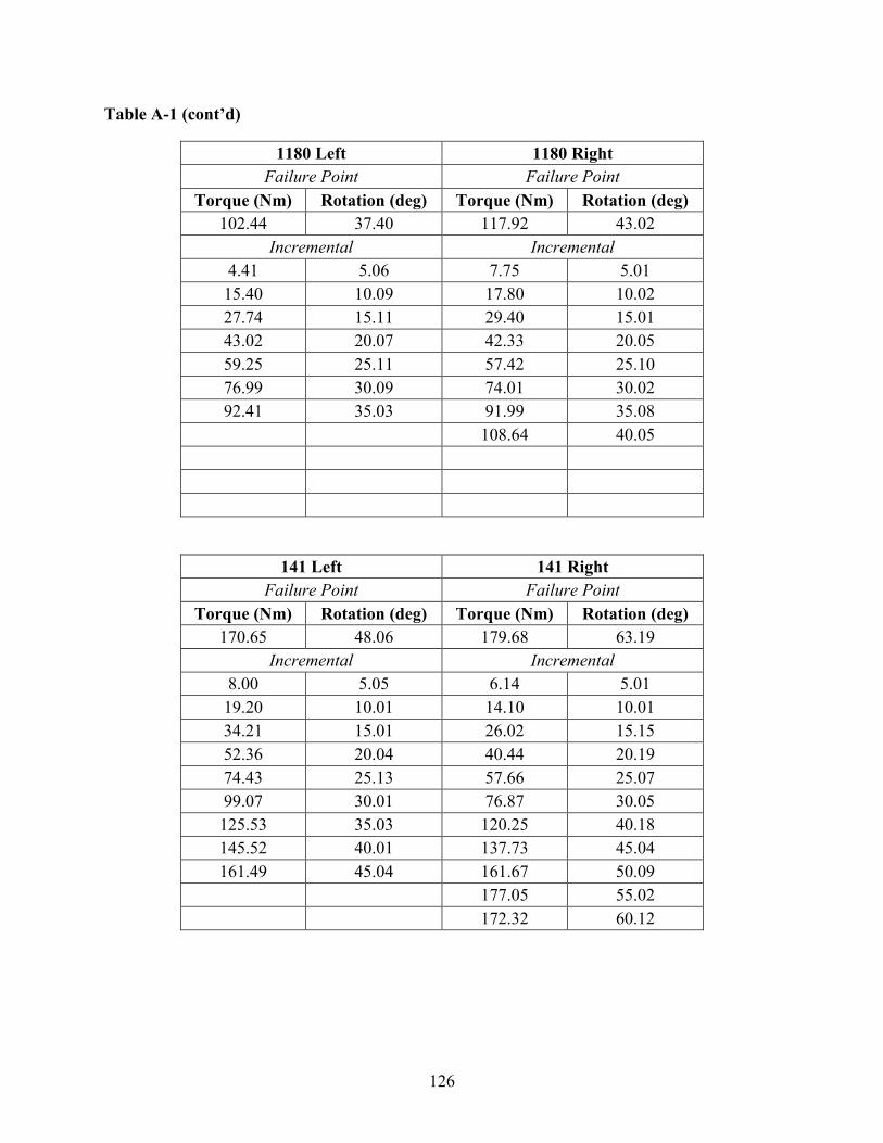
126

Table A-1 (cont’d)




102.44 37.40 117.92 43.02


4.41 5.06 7.75 5.01

15.40 10.09 17.80 10.02

27.74 15.11 29.40 15.01

43.02 20.07 42.33 20.05

59.25 25.11 57.42 25.10

76.99 30.09 74.01 30.02

92.41 35.03 91.99 35.08

108.64 40.05

141 Left 141 Right



170.65 48.06 179.68 63.19


8.00 5.05 6.14 5.01

19.20 10.01 14.10 10.01

34.21 15.01 26.02 15.15

52.36 20.04 40.44 20.19

74.43 25.13 57.66 25.07

99.07 30.01 76.87 30.05

125.53 35.03 120.25 40.18

145.52 40.01 137.73 45.04

161.49 45.04 161.67 50.09

177.05 55.02

172.32 60.12

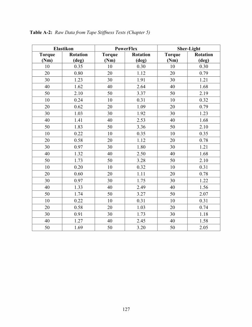
127

Table A-2: Raw Data from Tape Stiffness Tests (Chapter 5)

Elastikon PowerFlex Sher-Light

Torque

(Nm)

Rotation

(deg)

Torque

(Nm)

Rotation

(deg)

Torque

(Nm)

Rotation

(deg)

10 0.35 10 0.30 10 0.30

20 0.80 20 1.12 20 0.79

30 1.23 30 1.91 30 1.21

40 1.62 40 2.64 40 1.68

50 2.10 50 3.37 50 2.19

10 0.24 10 0.31 10 0.32

20 0.62 20 1.09 20 0.79

30 1.03 30 1.92 30 1.23

40 1.41 40 2.53 40 1.68

50 1.83 50 3.36 50 2.10

10 0.22 10 0.35 10 0.35

20 0.58 20 1.12 20 0.78

30 0.97 30 1.80 30 1.21

40 1.32 40 2.50 40 1.68

50 1.73 50 3.28 50 2.10

10 0.20 10 0.32 10 0.31

20 0.60 20 1.11 20 0.78

30 0.97 30 1.75 30 1.22

40 1.33 40 2.49 40 1.56

50 1.74 50 3.27 50 2.07

10 0.22 10 0.31 10 0.31

20 0.58 20 1.03 20 0.74

30 0.91 30 1.73 30 1.18

40 1.27 40 2.45 40 1.58

50 1.69 50 3.20 50 2.05

128

Table A-3: Input Motions for Computational Model (Chapter 5)

Tibia

Rotation

(deg)

Tape

Stiffness

(Nm/deg)

Talocrural

Dorsiflexion

(deg)

Talocrural

Rotation

(deg)

Talocrural

Eversion

(deg)

0 0 0.03 0.30 0.12

1 0 0.03 0.98 0.20

2 0 0.03 1.66 0.28

3 0 0.03 2.34 0.37

4 0 0.03 3.02 0.45

5 0 0.03 3.70 0.53

6 0 0.03 4.38 0.62

7 0 0.03 5.06 0.70

8 0 0.03 5.74 0.78

9 0 0.03 6.42 0.87

10 0 0.03 7.10 0.95

11 0 0.03 7.78 1.04

12 0 0.03 8.46 1.12

13 0 0.03 9.14 1.20

14 0 0.03 9.82 1.29

15 0 0.03 10.50 1.37

0 5 0.03 0.35 0.11

1 5 0.03 1.07 0.19

2 5 0.03 1.80 0.26

3 5 0.03 2.52 0.33

4 5 0.03 3.25 0.40

5 5 0.03 3.97 0.47

6 5 0.03 4.70 0.54

7 5 0.03 5.42 0.62

8 5 0.03 6.15 0.69

9 5 0.03 6.87 0.76

10 5 0.03 7.60 0.83

11 5 0.03 8.32 0.90

12 5 0.03 9.05 0.97

13 5 0.03 9.78 1.04

14 5 0.03 10.50 1.12

15 5 0.03 11.23 1.19

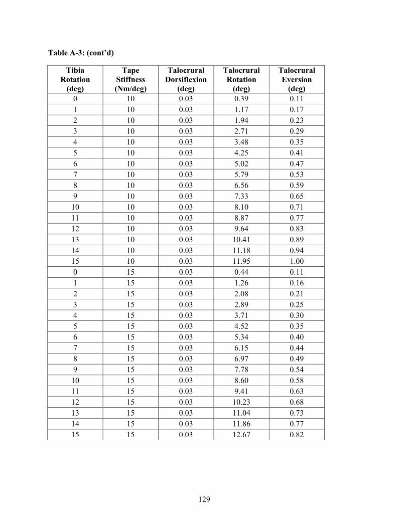
129

Table A-3: (cont’d)

Tibia

Rotation

(deg)

Tape

Stiffness

(Nm/deg)

Talocrural

Dorsiflexion

(deg)

Talocrural

Rotation

(deg)

Talocrural

Eversion

(deg)

0 10 0.03 0.39 0.11

1 10 0.03 1.17 0.17

2 10 0.03 1.94 0.23

3 10 0.03 2.71 0.29

4 10 0.03 3.48 0.35

5 10 0.03 4.25 0.41

6 10 0.03 5.02 0.47

7 10 0.03 5.79 0.53

8 10 0.03 6.56 0.59

9 10 0.03 7.33 0.65

10 10 0.03 8.10 0.71

11 10 0.03 8.87 0.77

12 10 0.03 9.64 0.83

13 10 0.03 10.41 0.89

14 10 0.03 11.18 0.94

15 10 0.03 11.95 1.00

0 15 0.03 0.44 0.11

1 15 0.03 1.26 0.16

2 15 0.03 2.08 0.21

3 15 0.03 2.89 0.25

4 15 0.03 3.71 0.30

5 15 0.03 4.52 0.35

6 15 0.03 5.34 0.40

7 15 0.03 6.15 0.44

8 15 0.03 6.97 0.49

9 15 0.03 7.78 0.54

10 15 0.03 8.60 0.58

11 15 0.03 9.41 0.63

12 15 0.03 10.23 0.68

13 15 0.03 11.04 0.73

14 15 0.03 11.86 0.77

15 15 0.03 12.67 0.82

130


Tibia

Rotation

(deg)

Tape

Stiffness

(Nm/deg)

Talocrural

Dorsiflexion

(deg)

Talocrural

Rotation

(deg)

Talocrural

Eversion

(deg)

0 20 0.03 0.49 0.11

1 20 0.03 1.35 0.15

2 20 0.03 2.21 0.18

3 20 0.03 3.07 0.22

4 20 0.03 3.94 0.25

5 20 0.03 4.80 0.29

6 20 0.03 5.66 0.32

7 20 0.03 6.52 0.36

8 20 0.03 7.38 0.39

9 20 0.03 8.24 0.43

10 20 0.03 9.10 0.46

11 20 0.03 9.96 0.50

12 20 0.03 10.82 0.53

13 20 0.03 11.68 0.57

14 20 0.03 12.54 0.60

15 20 0.03 13.40 0.64

0 25 0.03 0.54 0.11

1 25 0.03 1.45 0.13

2 25 0.03 2.35 0.16

3 25 0.03 3.26 0.18

4 25 0.03 4.16 0.20

5 25 0.03 5.07 0.23

6 25 0.03 5.97 0.25

7 25 0.03 6.88 0.27

8 25 0.03 7.78 0.29

9 25 0.03 8.69 0.32

10 25 0.03 9.60 0.34

11 25 0.03 10.50 0.36

12 25 0.03 11.41 0.38

13 25 0.03 12.31 0.41

14 25 0.03 13.22 0.43

15 25 0.03 14.12 0.45

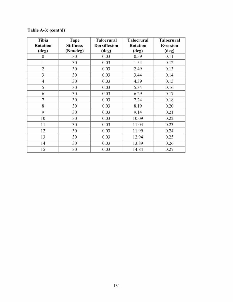
131


Tibia

Rotation

(deg)

Tape

Stiffness

(Nm/deg)

Talocrural

Dorsiflexion

(deg)

Talocrural

Rotation

(deg)

Talocrural

Eversion

(deg)

0 30 0.03 0.59 0.11

1 30 0.03 1.54 0.12

2 30 0.03 2.49 0.13

3 30 0.03 3.44 0.14

4 30 0.03 4.39 0.15

5 30 0.03 5.34 0.16

6 30 0.03 6.29 0.17

7 30 0.03 7.24 0.18

8 30 0.03 8.19 0.20

9 30 0.03 9.14 0.21

10 30 0.03 10.09 0.22

11 30 0.03 11.04 0.23

12 30 0.03 11.99 0.24

13 30 0.03 12.94 0.25

14 30 0.03 13.89 0.26

15 30 0.03 14.84 0.27

132

REFERENCES

133

REFERENCES

Attarian, D. E., McCrackin, H. J., Devito, D. P., McElhaney, J. H. & Garrett, W. E. 1985. A

biomechanical study of human lateral ankle ligaments and autogenous reconstructive grafts.

American Journal of Sports Medicine, 13.

Barbaix, E., Van Roy, P. & Clarys, J. P. 2000. Variations of anatomical elements contributing to

subtalar joint stability: intrinsic risk factors for post-traumatic lateral instability of the ankle.

Ergonomics, 43, 1718-1725.

Beumer, A., van Hemert, W. L. W., Swierstra, B. A., Jasper, L. E. & Belkoff, S. M. 2003. A

biomechanical evaluation of the tibiofibular and tibiotalar ligaments of the ankle. Foot & Ankle

International, 24.

Beynnon, B. D., Murphy, D. F. & Alosa, D. M. 2002. Predictive factors for lateral ankle sprains:

A literature review. Journal of Athletic Training, 37, 376-380.

Bonacci, J., Saunders, P. U., Hicks, A., Rantalainen, T., Vicenzino, B. T. & Spratford, W. 2013.

Running in a minimalist and lightweight shoe is not the same as running barefoot: a

biomechanical study. British Journal of Sports Medicine, 47, 387-392.

Boruta, P. M., Bishop, J. O., Braly, W. G. & Tullos, H. S. 1990. Acute ankle ligament injuries; a

literature review. Foot & Ankle, 11, 107-113.

Boytim, M. J., Fischer, D. A. & Neumann, L. 1991. Syndesmotic ankle sprains. American

Journal of Sports Medicine, 19.

Button, K., Braman, J., Davison, M., Wei, F., Schaeffer, M. & Haut, R. 2015. Rotational

stiffness of American football shoes affects ankle biomechanics and injury severity. Journal of

Biomechanical Engineering, 137(6), 061004.

Button, K. D., Wei, F., Meyer, E. G. & Haut, R. C. 2013. Specimen-Specific Computational

Models of Ankle Sprains Produced in a Laboratory Setting. Journal of Biomechanical

Engineering-Transactions of the ASME, 135.

Carson, M. C., Harrington, M. E., Thompson, N., O'Connor, J. J. & Theologis, T. N. 2001.

Kinematic analysis of a multi-segment foot model for research and clinical applications: a

repeatability analysis. Journal of Biomechanics, 34.

Cawley, P. W., Heidt, R. S., Scranton, P. E., Losse, G. M. & Howard, M. E. 2003. Physiologic

axial load, frictional resistance, and the football shoe-surface interface. Foot & Ankle

International, 24.

134

Chao, E. Y. S. 2003. Graphic-based musculoskeletal model for biomechanical analyses and

animation. Medical Engineering & Physics, 25, 201-212.

Cheung, J. T. M., An, K. N. & Zhang, M. 2006. Consequences of partial and total plantar fascia

release: A finite element study. Foot & Ankle International, 27, 125-132.

Colville, M. R., Marder, R. A., Boyle, J. J. & Zarins, B. 1990a. Strain measurement in lateral

ankle ligaments. American Journal of Sports Medicine, 18.

Colville, M. R., Marder, R. A., Boyle, J. J. & Zarins, B. 1990b. Strain-measurement in lateral

ankle ligaments. American Journal of Sports Medicine, 18.

Crandall, J., Portier, L., Petit, P. & Hall, G. 1996. Biomechanical response and physical

properties of the leg, foot, and ankle.) 40th Stapp Car Crash Conference.

Dattani, R., Patnaik, S., Kantak, A., Srikanth, B. & Selvan, T. P. 2008. Injuries to the tibiofibular

syndesmosis. Journal of Bone and Joint Surgery-British Volume, 90B.

Delahunt, E., Monaghan, K. & Caulfield, B. 2006. Altered neuromuscular control and ankle joint

kinematics during walking in subjects with functional instability of the ankle joint. American

Journal of Sports Medicine, 34, 1970-1976.

Dias, L. S. 1979. Lateral ankle sprain: An experimental study. Journal of Trauma-Injury

Infection and Critical Care, 19, 266-269.

Dubin, J. C., Comeau, D., McClelland, R. I., Dubin, R. A. & Ferrel, E. 2011. Lateral and

syndesmotic ankle sprain injuries: a narrative literature review. Journal of Chiropractic

Medicine, 10, 204-19.

Edwards, G. S. & Delee, J. C. 1984. Ankle diastasis without fracture. Foot & Ankle, 4.

Elmore KA 2012. Soft tissue structures resisting anterior instability in a computational

glenohumeral joint model.

Fallat, L., Grimm, D. J. & Saracco, J. A. 1998. Sprained ankle syndrome: prevalence and

analysis of 639 acute injuries. The Journal of foot and ankle surgery : Official Publication of the

American College of Foot and Ankle Surgeons, 37, 280-5.

Fassbind, M. J., Rohr, E. S., Hu, Y., Haynor, D. R., Siegler, S., Sangeorzan, B. J. & Ledoux, W.

R. 2011. Evaluating Foot Kinematics Using Magnetic Resonance Imaging: From Maximum

Plantar Flexion, Inversion, and Internal Rotation to Maximum Dorsiflexion, Eversion, and

External Rotation. Journal of Biomechanical Engineering-Transactions of the ASME, 133.

Fong, D. T.-P., Ha, S. C.-W., Mok, K.-M., Chan, C. W.-L. & Chan, K.-M. 2012. Kinematics

Analysis of Ankle Inversion Ligamentous Sprain Injuries in Sports Five Cases From Televised

Tennis Competitions. American Journal of Sports Medicine, 40, 2627-2632.

135

Fong, D. T.-P., Hong, Y., Chan, L.-K., Yung, P. S.-H. & Chan, K.-M. 2007. A systematic review

on ankle injury and ankle sprain in sports. Sports Medicine, 37, 73-94.

Fong, D. T.-P., Wei, F., Hong, Y., Krosshaug, T., Haut, R. C. & Chan, K.-M. 2011. Ankle

ligament strain during supination sprain injury–a computational biomechanics study.) ISBS-

Conference.

France, E. P., Paulos, L. E., Abbott, P. J., Roberts, P. F., Muhic, L. A., Lemaster, J. H. &

Kazarian, L. E. 1987. Failure characteristics of the medial collateral ligament of the knee -

effects of high-strain rate. Aviation Space and Environmental Medicine, 58.

Funk, J. R., Hall, G. W., Crandall, J. R. & Pilkey, W. D. 2000. Linear and quasi-linear

viscoelastic characterization of ankle ligaments. Journal of Biomechanical Engineering-

Transactions of the ASME, 122.

Funk, J. R., Srinivasan, S. C. M., Crandall, J. R., Khaewpong, N., Eppinger, R. H., Jaffredo, A.

S., Potier, P. & Petit, P. Y. 2002. The effects of axial preload and dorsiflexion on the tolerance of

the ankle/subtalar joint to dynamic inversion and eversion. Stapp Car Crash Journal, 46, 245-65.

Garrick, J. G. & Requa, R. K. 1989. The epidemiology of foot and ankle injuries in sports.

Clinics in Podiatric Medicine and Surgery, 6, 629-37.

Gerber, J. P., Williams, G. N., Scoville, C. R., Arciero, R. A. & Taylor, D. C. 1998. Persistent

disability associated with ankle sprains: A prospective examination of an athletic population.

Foot & Ankle International, 19.

Golano, P., Vega, J., de Leeuw, P. A. J., Malagelada, F., Cristina Manzanares, M., Gotzens, V. &

van Dijk, C. N. 2010. Anatomy of the ankle ligaments: a pictorial essay. Knee Surgery Sports

Traumatology Arthroscopy, 18, 557-569.

Guise, E. R. 1976. Rotational ligamentous injuries to the ankle in football. The American Journal

of Sports Medicine, 4.

Haraguchi, N. & Armiger, R. S. 2009. A New Interpretation of the Mechanism of Ankle

Fracture. Journal of Bone and Joint Surgery-American Volume, 91A.

Harper, M. C. 1992. Ankle fracture classification systems: a case for integration of the Lauge-

Hansen and AO-Danis-Weber schemes. Foot & ankle, 13, 404-7.

Heilman, A. E., Braly, W. G., Bishop, J. O., Noble, P. C. & Tullos, H. S. 1990. An anatomic

study of subtalar instability. Foot & Ankle, 10, 224-228.

Hennig, E. M. 2011. The Influence of Soccer Shoe Design on Player Performance and Injuries.

Research in Sports Medicine, 19, 186-201.

136

Hertel, J., Denegar, C. R., Monroe, M. M. & Stokes, W. L. 1999. Talocrural and subtalar joint

instability after lateral ankle sprain. Medicine and Science in Sports and Exercise, 31, 1501-

1508.

Hicks, J. H. 1953. The mechanics of the foot: 1. the joints. Journal of Anatomy, 87, 345-357.

Hirsch, C. & Lewis, J. 1965. Experimental ankle-joint fractures. Acta Orthopaedica

Scandinavica, 36, 408-&.

Holzbaur, K. R. S., Murray, W. M. & Delp, S. L. 2005. A model of the upper extremity for

simulating musculoskeletal surgery and analyzing neuromuscular control. Annals of Biomedical

Engineering, 33, 829-840.

Hootman, J. M., Dick, R. & Agel, J. 2007. Epidemiology of collegiate injuries for 15 sports:

Summary and recommendations for injury prevention initiatives. Journal of Athletic Training,

42.

Hopkinson, W. J., Stpierre, P., Ryan, J. B. & Wheeler, J. H. 1990. Syndesmosis sprains of the

ankle. Foot & Ankle, 10.

Hughes, J. L., Weber, H., Willenegger, H. & Kuner, E. H. 1979. Evaluation of ankle fractures:

non-operative and operative treatment. Clinical Orthopaedics and Related Research, 111-119.

Iaquinto, J. M. & Wayne, J. S. 2010. Computational model of the lower leg and foot/ankle

complex: application to arch stability. Journal of Biomechanical Engineering, 132.

Kato, T. 1995. The diagnosis and treatment of instability of the subtalar joint. Journal of Bone

and Joint Surgery-British Volume, 77B, 400-406.

Kent, R., Crandall, J., Forman, J., Lessley, D., Lau, A. & Garson, C. 2012. Development and

assessment of a device and method for studying the mechanical interactions between shoes and

playing surfaces in situ at loads and rates generated by elite athletes. Sports Biomechanics, 11,

414-429.

Kitaoka, H. B., Luo, Z. P. & An, K. N. 1997. Three-dimensional analysis of normal ankle and

foot mobility. American Journal of Sports Medicine, 25, 238-242.

Kleipool, R. P. & Blankevoort, L. 2010. The relation between geometry and function of the

ankle joint complex: a biomechanical review. Knee Surgery Sports Traumatology Arthroscopy,

18, 618-627.

Konradsen, L. & Voigt, N. 2002. Inversion injury biomechanics in functional ankle instability: a

cadaver study of simulated gait. Scandinavian Journal of Medicine & Science in Sports, 12.

137

Krosshaug, T. & Bahr, R. 2005. A model-based image-matching technique for three-dimensional

reconstruction of human motion from uncalibrated video sequences. Journal of Biomechanics,

38, 919-929.

Kuhlman, S., Sabick, M., Pfeiffer, R., Cooper, B. & Forhan, J. 2010. Effect of loading condition

on the traction coefficient between shoes and artificial turf surfaces. Proceedings of the

Institution of Mechanical Engineers Part P-Journal of Sports Engineering and Technology, 224,

155-165.

Kwak, S., Blakevoort, L. & Ateshian, G. 2000. A mathematical formulation for 3D quasi-static

multibody models of diarthrodial joints. Computer Methods in Biomechanics and Biomedical

Engineering, 3, 41-64.

Kwon, J. Y., Chacko, A. T., Kadzielski, J. J., Appleton, P. T. & Rodriguez, E. K. 2010. A Novel

Methodology for the Study of Injury Mechanism: Ankle Fracture Analysis Using Injury Videos

Posted on YouTube.com. Journal of Orthopaedic Trauma, 24, 477-482.

Lambson, R. B., Barhnill, B. S. & Higgins, R. W. 1996. Football cleat design and its effect on

anterior cruciate ligament injuries - A three-year prospective study. American Journal of Sports

Medicine, 24, 155-159.

Laugehansen, N. 1950. Fractures of the Ankle. Archives of Surgery, 60.

Leardini, A., Stagni, R. & O'Connor, J. J. 2001. Mobility of the subtalar joint in the intact ankle

complex. Journal of Biomechanics, 34, 805-809.

Liacouras, P. C. & Waynel, J. S. 2007. Computational modeling to predict mechanical function

of joints: Application to the lower leg with simulation of two cadaver studies. Journal of

Biomechanical Engineering-Transactions of the ASME, 129, 811-817.

Lin, C. F., Gross, M. T. & Weinhold, P. 2006. Ankle syndesmosis injuries: Anatomy,

biomechanics, mechanism of injury, and clinical guidelines for diagnosis and intervention.

Journal of Orthopaedic & Sports Physical Therapy, 36.

Livesay, G. A., Reda, D. R. & Nauman, E. A. 2006. Peak torque and rotational stiffness

developed at the shoe-surface interface - The effect of shoe type and playing surface. American

Journal of Sports Medicine, 34.

Loram, I. D. & Lakie, M. 2002. Direct measurement of human ankle stiffness during quiet

standing: the intrinsic mechanical stiffness is insufficient for stability. Journal of Physiology-

London, 545, 1041-1053.

Lundberg, A., Svensson, O. K., Bylund, C., Goldie, I. & Selvik, G. 1989a. Kinematics of the

ankle/foot complex--part 2: pronation and supination. Foot & Ankle, 9, 248-253.

138

Lundberg, A., Svensson, O. K., Bylund, C. & Selvik, G. 1989b. Kinematics of the foot/ankle

complex--part 3: influence of leg rotation. Foot & Ankle, 9, 304-309.

Meyers, M. C. 2010. Incidence, Mechanisms, and Severity of Game-Related College Football

Injuries on FieldTurf Versus Natural Grass A 3-Year Prospective Study. American Journal of

Sports Medicine, 38, 687-697.

Miller, C. D., Shelton, W. R., Barrett, G. R., Savoie, F. H. & Dukes, A. D. 1995. Deltoid and

syndesmotic ligament injury of the ankle without fracture. American Journal of Sports Medicine,

23.

Mok, K.-M., Fong, D. T.-P., Krosshaug, T., Engebretsen, L., Hung, A. S.-L., Yung, P. S.-H. &

Chan, K.-M. 2011. Kinematics Analysis of Ankle Inversion Ligamentous Sprain Injuries in

Sports 2 Cases During the 2008 Beijing Olympics. American Journal of Sports Medicine, 39.

Netter, F. H. & JT, H. 2003. Atlas of Human Anatomy, Teterboro, NJ, Icon Learning Systems.

Ng, B. H., Chou, S. M., Lim, B. H. & Chong, A. 2004. Strain rate effect on the failure properties

of tendons. Proceedings of the Institution of Mechanical Engineers Part H-Journal of

Engineering in Medicine, 218.

Nigg, B. M. & Yeadon, M. R. 1987. Biomechanical aspects of playing surfaces. Journal of

Sports Sciences, 5.

Norkus, S. A. & Floyd, R. T. 2001. The anatomy and mechanisms of syndesmotic ankle sprains.

Journal of Athletic Training, 36.

Parenteau, C. S., Viano, D. C. & Petit, P. Y. 1998. Biomechanical properties of human cadaveric

ankle-subtalar joints in quasi-static loading. Journal of Biomechanical Engineering-Transactions

of the ASME, 120, 105-111.

Peltz, C. D., Haladik, J. A., Hoffman, S. E., McDonald, M., Ramo, N. L., Divine, G., Nurse, M.

& Bey, M. J. 2014. Effects of footwear on three-dimensional tibiotalar and subtalar joint motion

during running. Journal of Biomechanics, 47, 2647-53.

Petit, P. 1996. Quasi-static Characterization of the human foot-ankle joints in a simulated tensed

state and updated accidentological data.) IRCOBI.

Rasmussen, O. & Kromannandersen, C. 1983. Experimental ankle injuries--Analysis of the

traumatology of the ankle ligaments. Acta Orthopaedica Scandinavica, 54, 356-362.

Renstrom, P. & Konradsen, L. 1997. Ankle ligament injuries. British Journal of Sports Medicine,

31.

Safran, M. R., Benedetti, R. S., Bartolozzi, A. R. & Mandelbaum, B. R. 1999. Lateral ankle

sprains: a comprehensive review - Part 1: etiology, pathoanatomy, histopathogenesis, and

diagnosis. Medicine and Science in Sports and Exercise, 31.

139

Sarsam, I. M. & Hughes, S. P. F. 1988. The role of the anterior tibiofibular ligament in talar

rotation: an anatomical study. Injury, 19, 62-64.

Siegler, S., Chen, J. & Schneck, C. D. 1988. The 3-dimensional kinematics and flexibility

characteristics of the human ankle and subtalar joints--part 1: kinematics. Journal of

Biomechanical Engineering-Transactions of the ASME, 110, 364-373.

Smith, A. W. & Wong, D. P. 2012. Effects of window size on ankle joint stiffness calculation

during quiet standing: How the rule changes the result. Journal of Biomechanics, 45, 2301-2305.

Soutas-Little, R. W., Beavis, G. C., Verstraete, M. C. & Markus, T. L. 1987. Analysis of Foot

Motion During Running Using a Joint-Coordinate System. Medicine and Science in Sports and

Exercise, 19.

Torg, J. S. & Quedenfe.Tc 1973. Effect of shoe type and cleat length on incidence and severity

of knee injuries among high school football players. Journal of Bone and Joint Surgery-

American Volume, A 55, 1319-1319.

Vanlangelaan, E. J. 1983. A kinematical analysis of the tarsal joints. Acta Orthopaedica

Scandinavica, 54, 11-269.

Viladot, A., Lorenzo, J. C., Salazar, J. & Rodriguez, A. 1984. The subtalar joint-embryology and

morphology. Foot & Ankle, 5, 54-66.

Villwock, M. R., Meyer, E. G., Powell, J. W., Fouty, A. J. & Haut, R. C. 2009a. Football Playing

Surface and Shoe Design Affect Rotational Traction.

Villwock, M. R., Meyer, E. G., Powell, J. W., Fouty, A. J. & Haut, R. C. 2009b. Football Playing

Surface and Shoe Design Affect Rotational Traction. American Journal of Sports Medicine, 37.

Villwock, M. R., Meyer, E. G., Powell, J. W. & Haut, R. C. 2009c. Development and evaluation

of a surrogate ankle for use with a rotational traction measurement apparatus. Proceedings of the

Institution of Mechanical Engineers Part P-Journal of Sports Engineering and Technology, 223.

Vitale, T. D. & Fallat, L. M. 1988. Lateral ankle sprains: evaluation and treatment. The Journal

of Foot Surgery, 27.

Waterman, B. R., Belmont, P. J., Jr., Cameron, K. L., DeBerardino, T. M. & Owens, B. D. 2010.

Epidemiology of Ankle Sprain at the United States Military Academy. American Journal of

Sports Medicine, 38.

Waterman, B. R., Belmont, P. J., Jr., Cameron, K. L., Svoboda, S. J., Alitz, C. J. & Owens, B. D.

2011. Risk Factors for Syndesmotic and Medial Ankle Sprain Role of Sex, Sport, and Level of

Competition. American Journal of Sports Medicine, 39.

140

Weaver, B., Fitzsimons, K., Braman, J. & Haut, R. 2013. Torque prediction at the shoe-surface

interface using insole pressure technology. Journal of Sports Engineering and Technology, In

Print.

Wei, F., Braman, J., Meyer, E., Powell, J. & Haut, R. 2011a. Mechanism of injury in a high

ankle sprain: A simulation study.) Summer Bioengineering Conference. Farmington, PA.

Wei, F., Braman, J. E., Weaver, B. T. & Haut, R. C. 2011c. Determination of dynamic ankle

ligament strains from a computational model driven by motion analysis based kinematic data.

Journal of Biomechanics, 44, 2636-2641.

Wei, F., Hunley, S. C., Powell, J. W. & Haut, R. C. 2011d. Development and Validation of a

Computational Model to Study the Effect of Foot Constraint on Ankle Injury due to External

Rotation. Annals of Biomedical Engineering, 39.

Wei, F., Meyer, E. G., Braman, J. E., Powell, J. W. & Haut, R. C. 2012a. Rotational Stiffness of

Football Shoes Influences Talus Motion during External Rotation of the Foot. Journal of

Biomechanical Engineering-Transactions of the ASME, 134.

Wei, F., Post, J. M., Braman, J. E., Meyer, E. G., Powell, J. W. & Haut, R. C. 2012b. Eversion

during external rotation of the human cadaver foot produces high ankle sprains. Journal of

Orthopaedic Research, 30.

Wei, F., Villwock, M. R., Meyer, E. G., Powell, J. W. & Haut, R. C. 2010. A Biomechanical

Investigation of Ankle Injury Under Excessive External Foot Rotation in the Human Cadaver.

Journal of Biomechanical Engineering-Transactions of the ASME, 132.

Williams, D. S. B., 3rd, Green, D. H. & Wurzinger, B. 2012. Changes in lower extremity

movement and power absorption during forefoot striking and barefoot running. International

Journal of Sports Physical Therapy, 7, 525-32.

Williams, G. N., Jones, M. H. & Amendola, A. 2007. Syndesmotic ankle sprains in athletes.

American Journal of Sports Medicine, 35.

Wolfe, M. W., Uhl, T. L., Mattacola, C. G. & McCluskey, L. C. 2001. Management of ankle

sprains (vol 63, pg 93, 2001). American Family Physician, 64.

Wong, Y. S., Kim, W. & Ying, N. 2005. Passive motion characteristics of the talocrural and the

subtalar joint by dual Euler angles. Journal of Biomechanics, 38, 2480-2485.

Wu, G., Siegler, S., Allard, P., Kirtley, C., Leardini, A., Rosenbaum, D., Whittle, M., D'Lima, D.

D., Cristofolini, L., Witte, H., Schmid, O. & Stokes, H. 2002. ISB recommendation on

definitions of joint coordinate system of various joints for the reporting of human joint motion -

part 1: ankle, hip, and spine. Journal of Biomechanics, 35, 543-548.

141

Yahia, L., Brunet, J., Labelle, S. & Rivard, C. H. 1990. A scanning electron-microscopic study

of rabbit ligaments under strain. Matrix, 10.

Yeung, M. S., Chan, K. M., So, C. H. & Yuan, W. Y. 1994. An epidemiological survey on ankle

sprain. British Journal of Sports Medicine, 28, 112-116.

BIOMECHANICAL RESPONSE OF THE ANKLE TO EXCESSIVE EXTERNAL ROTATION …2694/... · ·...

Documents

Transcript of BIOMECHANICAL RESPONSE OF THE ANKLE TO EXCESSIVE EXTERNAL ROTATION …2694/... · ·...