Bioactive lipids in plasma

The effect of acrolein and biodiesel exhaust exposure on the endocannabinoid levels in human plasma and method development for future analysis of oxylipins

Michelle Maier

Michelle Maier

Degree Thesis in Chemistry 30 ECTS

Master’s Level

Report passed: August 8, 2013

Supervisors: Malin L. Nording, Sandra Gouveia

Examiner: Patrik Andersson

I

Abstract

Oxylipins and endocannabinoids are classes of fatty acid metabolites acting on receptors and ion-channels in the body and therefore playing a role as biomarkers for certain pathological or physiological processes including inflammation, pain, cancer and stress, among others. The overall goal of this thesis was to apply a previously developed and validated ultra-performance liquid chromatography-electrospray tandem mass spectrometry (UPLC-ESI/MS/MS) method for the analysis of endocannabinoids in human plasma obtained from subjects taking part in two different studies, the acrolein exposure and the biodiesel exhaust exposure study, with samples being collected at different time points. Both studies were carried out in collaboration with other departments. Our specific aim was to find out if there are any differences in temporal endocannabinoid levels when either being exposed to acrolein, biodiesel exhaust or diesel exhaust. The applied method was developed with high sensitivity and with the ability to detect and quantify 15 endocannabinoids simultaneosly. Sample preparation involved solid phase extraction (SPE) to remove any matrix effects caused by human plasma. Liquid chromatograhic separation was performed using a Waters Acquity UltraPerformance with water and methanol with 10 mM Ch3CHOONH4 as mobile phases under gradient conditions. Mass detection was performed using a Quattro Ultima Micromass in positive electron spray ionization mode. 11 out of 15 endocannabinoids were detected and quantified in all human plasma samples obtained from the two studies and at different timepoints. Endocannabinoid levels ranged from 6 pg to 94 ng per mL plasma obtained from the acrolein exposure study. Endocannabinoid levels ranged from 4 pg to 31 ng per mL plasma obtained from the biodiesel exhaust exposure study. Since no further statistical tests were carried out during the course of the diploma project, it was not possible to draw definite conclusions regarding the significance of increasing or decreasing amounts in response to exposure of acrolein or biodiesel exhaust. In general there were trends, which can also be seen when for example multivariate data analysis of the acrolein exposure study results was performed. To entirely confirm any speculations regarding changes in endocannabinoid levels before and after any exposure it is therefore necessary to conduct stastistical tests, which will be done with the obtained data results after this project has been completed. A further aim of the thesis was to develop a highly selective and sensitive UPLC-ESI/MS/MS method for the simultaneous analysis of 16 oxylipins. In future research, this method will be applied for the analysis of oxylipins in the human plasma samples obtained from these two studies. Liquid chromatograhic separatation was performed using a Waters Acquity UltraPerformance with water with 0.1% glacial acetic acid and acetonitrile/methanol 85:15 (v/v) with 0.1% glacial acetic acid as mobile phases under gradient conditions. Mass detection was performed using a Quattro Ultima Micromass in negative electron spray ionization mode. Limit of quantification values between 28 pg and 18 ng on column, R2 values between 0.9739 and 0.9998 and average recoveries of the internal standards in plasma between 50% and 99% with exception of 12(13)-EpOME-d4 with average recoveries of 14% and 26% were obtained. Interday and intraday precision was <15% and accuracy >80%. The findings of the endocannabinoid levels in human plasma obtained from the two studies suggest that the endocannabinoid profiling platform can be applied in a broad range of biological samples to study bioactive lipids more closely in relation to the body’s reaction and in particular to human diseases. It is likely that this applies to the class of oxylipins as well, which is why they will also be analyzed with the validated method in biological matrices in future research.

II

III

List of abbreviations

ARA Arachidonic acid ACN Acetonitrile AEA Arachidonoyl Ethanolamide or Anandamide 1-AG 1-Arachidonoyl Glycerol 2-AG 2-Arachidonoyl Glycerol 2-AGe 2-arachidonoyl glycerol ether or Noladin ALA α-linolenic acid BEH Ethylene bridged hybrid CAP Capillary voltage CB1/CB2 Cannabinoid receptor type 1/type 2 CE Collision energy COX Enzyme Cyclooxygenase CV Colume volume. It corresponds to 4 mL. CV Cone voltage CYP Enzyme Cytochrome P450 DC Direct current DEA Docosatetraenoyl Ethanolamide DGLA Dihomo-γ-linolenic acid DHA Docosahexaenoic acid DHEA Docosahexaenoyl Ethanolamide DHETs Dihydroxyeicosatrienoic acids DTA Docosatetraenoic acid EC(s) Endocannabinoid(s) EpETrEs Epoxyeicosatrienoic acids EPA Eicopentaenoic acid ETA Eicosatrienoic acid EPEA Eicosapentaenoyl Ethanolamide ESI Electrospray ionization FAAH Enzyme Fatty-Acid amide Hydrolase FDA Food and Drug administration GC Gas chromatography GPR55 Orphan G-coupled receptor HETEs Hydroxyeicosatetraenoic acids HLB Hydrophilic-lipophilic balance 5-HPETE 5-hydroperoxyeicosatetraenoic acid HPLC High-performance liquid chromatography ICH International Conference for Harmonization IS Internal standard 8-iso-PGE2 8-iso Prostaglandin E2 8-iso-PGF2α 8-iso Prostaglandin F2α LA Linoleic acid 2-LG 2-Linoleoyl Glycerol LC Liquid chromatography LEA Linoleoyl Ethanolamide LOD Limit of detection LOX Enzyme Lipoxygenase LOQ Limit of quantification MAGL Monoacylglycerol Lipase MRM Multiple reaction monitoring MS Mass spectrometry NADA N-Arachidonoyl Dopamine NAGly Arachidonoyl Glycine O-AEA O-arachidonoyl Ethanolamide or Virodhamine

IV

OEA Oleoyl Ethanolamide OLA Oleic acid OPLS Orthogonal projections to latent structures OPLS-DA Orthogonal projections to latent structures using discriminant

analysis PA Palmitic acid PAHs Polycyclic aromatic hydrocarbons PBS Phosphate buffer saline PC Principal component PCA Principal component analysis PEA Palmitoyl Ethanolamide or Palmidrol PGD2 Prostaglandin D2 PGE2 Prostaglandin E2

PGH2 Prostaglandin H2

PLA2 Enzyme Phospholipase A2 PLS Partial least squares projections to latent structures POA Palmitoleic acid POEA Palmitoleoyl Ethanolamide Q2 Goodness of prediction Ratio AStd/AIS Ratio of standard area to internal standard area ROS Reactive Oxygen Species R2 Goodness of fit RF Radio frequency RT Retention time SEA Stearoyl Ethanolamide sEH Soluble epoxide hydrolase SPE Solid phase extraction STD Standard TRPV1 Transient receptor potential vanilloid type 1 TXB2 Thromboxane B2 UPLC Ultra-performance liquid chromatography UPLC-ESI/MS/MS Ultra-performance liquid chromatography-electrospray

tandem mass spectrometry

V

Table of contents

Abstract .......................................................................................................................... I List of abbreviations ................................................................................................... III 1. Introduction ............................................................................................................... 1

1.1 Aim of the diploma work ...................................................................................... 1 1.2 Bioactive lipids ..................................................................................................... 1

1.2.1 Oxylipins ........................................................................................................ 1 1.2.2 Endocannabinoids ......................................................................................... 5

1.3 Instrumentation ................................................................................................... 7 1.3.1 Solid phase extraction .................................................................................... 8 1.3.2 Ultra-performance liquid chromatography (UPLC) ..................................... 8 1.3.3 Mass spectrometry (MS) ............................................................................... 8 1.3.4 Quantification by the internal standard method and recovery calculations 9

1.4 Developing and validating an UPLC-MS/MS method ........................................ 11 1.5 Multivariate data analysis .................................................................................. 12 1.6 Acrolein exposure study ..................................................................................... 12 1.7 Biodiesel exhaust exposure study ....................................................................... 13

2. Material and Methods .............................................................................................. 15 2.1 Chemicals ........................................................................................................... 15 2.2 Method development for oxylipin quantification by LC/MS ............................ 15 2.3 Oxylipin method validation ............................................................................... 16

2.3.1 Linearity and LOQ ....................................................................................... 16 2.3.2 Recovery for SPE extraction ....................................................................... 16 2.3.3 Inter- and intraday precision and accuracy ................................................ 17

2.4 Endocannabinoid quantification ....................................................................... 17 2.4.1 Standard stock solution preparation ........................................................... 19 2.4.2 Native standard curve preparation ............................................................. 19 2.4.3 Internal standard curve preparation .......................................................... 19 2.4.4 Sample preparation process for acrolein exposure and biodiesel exhaust exposure experiments ......................................................................................... 20

2.5 Application of the UPLC-ESI/MS/MS method for quantification of endocannabionoids in human plasma ..................................................................... 21

2.5.1 Experimental design of the acrolein exposure study .................................. 21 2.5.2 Experimental design of the biodiesel exhaust exposure study ................... 22

2.6 Multivariate data analysis .................................................................................. 23 3. Results and Discussion ............................................................................................ 24

3.1 Oxylipin method validation parameters ............................................................ 24 3.2 Endocannabinoid profiling of plasma samples from the acrolein exposure study .................................................................................................................................. 29

3.2.1 Multivariate data analysis for acrolein exposure study results ................... 35 3.3 Endocannabinoid profiling of plasma samples from the biodiesel exhaust exposure study ......................................................................................................... 36 3.4 Summary and comparison of acrolein exposure and biodiesel exhaust exposure results with relation to aim of study ........................................................................ 41

4. Conclusions .............................................................................................................. 44 5. Future perspectives .................................................................................................. 45 Acknowledgements ...................................................................................................... 46 References .................................................................................................................... 47 Appendix

VI

1

1. Introduction

1.1 Aim of the diploma work The diploma work focused on two groups of fatty acid metabolites, oxylipins and endocannabinoids (EC), functioning as bioactive lipids. The overall goal was to:

i. develop and validate an ultra-performance liquid chromatography-electrospray tandem mass spectrometry (UPLC-ESI/MS/MS) method for oxylipin analysis, and

ii. apply a previously validated UPLC-ESI/MS/MS method for endocannabinoid analysis.

The validated UPLC-ESI/MS/MS method for analysis of endocannabinoids was applied to human plasma samples, prepared by solid phase extraction (SPE), obtained from two exposure studies, the acrolein exposure study and the biodiesel exhaust exposure study in collaboration with the Department of Psychology and the Department of Public Health and Clinical Medicine at Umeå University. The specific aim of the acrolein exposure study was to distinguish differences between the endocannabinoid levels before and after exposure with acrolein. Our hypothesis was that chemical sensitive subjects react differently to irritants such as acrolein than healthy subjects, and that this can also be reflected in metabolite profiles. The specific aim of the biodiesel exhaust exposure study was to investigate the endocanabinoid levels in healthy subjects at different time points before and after exposure to test the hypothesis that biodiesel is less harmful to humans than diesel exhaust, as it was first suggested when introducing biodiesel fuels. For this purpose, cardiovascular, respiratory and inflammatory responses were also investigated by our collaborators.

1.2 Bioactive lipids The research field on bioactive lipids has been emerging in the last decades. This has occurred rather slowly since lipids have previously only been considered to be energy sources or components of cell membranes in the body. On the contrary, bioactive lipids are lipids that activate certain signaling pathways in our body in response to extracellular stimuli. They are produced through certain biosynthethic pathways from membrane lipids or from dietary precursors such as amino acids etc. (1). After being synthesized, they are exported into the extracellular system and bound to their receptors in order to transfer signals to target cells. Bioactive lipids are therefore also called lipid mediators and play an important role in many biological processes. An imbalance of lipid mediator signaling pathways is often linked to various reactions of the body or diseases such as inflammation, infertility, arteriosclerosis, ischemia, metabolic syndrome and cancer (2). Bioactive lipid research now focuses on a wide variety of compounds including phospho- and sphingolipids, oxylipins and endocannabinoids with the aim to discover more about the lipid signaling pathways in the body (2). Endocannabinoids and oxylipins, which the thesis focuses on, are introduced in the following sections.

1.2.1 Oxylipins

Oxylipins are a family of oxidized metabolites of polyunsaturated fatty acids, acting as lipid mediators and carrying out a variety of functions (3). All oxylipins have similar

2

structures, chemistries and physical properties, making the identification and quantification of the isomers challenging. Furthermore, oxylipins can only be found in very low concentrations, with varying concentrations by more than three fold (4,5). Oxylipins, derived from 20-carbon arachidonic acid (ARA), are also called eicosanoids. These eicosanoids include prostaglandins, leukotrienes, lipoxins, prostacyclin, thromboxanes, hydroxyeicosatetraenoic acids (HETEs) and epoxyeicosatrienoic acids (EpETrEs) (5). The best characterized are prostaglandins and leukotrienes (4). ARA is primarily a component of membrane phospholipids and can be released by the enzyme phospholipase A2 (PLA2). In addition, it can be formed from diacylglycerol by diacylglycerol lipase (6). It is then converted to oxylipins by cyclooxygenase (COX), lipoxygenase (LOX), cytochrome P450 (CYP) and reactive oxygen species (ROS) (6). COX catalyzation leads to the formation of prostaglandin H2 (PGH2), which acts as a precursor for prostacyclin, prostaglandins and thromboxanes. The enzyme 5-lipoxygenase (5-LOX) catalyzes the creation of 5-hydroperoxyeicosatetraenoic acid (5-HPETE). This metabolite is then transformed to leukotrienes and lipoxins. CYPs catalyze the conversion of ARA to hydroxyeicosatetraenoic acids (HETEs) and the conversion of ARA to EpETrES which are then transformed to dihydroxyeicosatrienoic acids (DHETs) by soluble epoxide hydrolase (sEH) (6).

Oxylipins, such as eicosanoids, are referred to as regulatory lipids because they are mediators that regulate different physiological processes including apoptosis, cell proliferation, tissue repair, blood clotting, blood vessel permeability, inflammation, immune cell behavior etc. (5). A disturbance in the level of eicosanoids can be associated with different diseases such as cardiovascular disease, stroke, myocardial infarction, asthma, Crohn’s disease, hypertension and cancer (6). Some have pro-inflammatory, some anti-inflammatory properties, and also play a part in the initiation and resolution of inflammation (7). Even though the oxylipins originating from ARA have been extensively researched and the catabolic pathways are the target of more than 75% of the world’s pharmaceuticals (5), other unsaturated fatty acids such as docosahexaenoic acid (DHA), linoleic acid (LA), dihomo-γ-linolenic acid (DGLA), α-linolenic acid (ALA), eicosatrienoic acid (ETA) and eicopentaenoic acid (EPA) can also undergo the above mentioned enzymatic conversions. Non-enzymatic conversions are possible as well (7). Therefore these metabolites can also contribute to the understanding of diseases (3). A schematic overview of fatty acid precursors and their oxylipin products can be found in figure 1. Figure 2 shows the molecular structures of the oxylipins selected for method development and validation.

An example of a pathway studied more closely, in addition to COX- and LOX-pathways, is the conversion of EpETrEs by the α/β hydrolase fold enzyme sEH to their less biologically active compounds, vicinal diols, DHETS. EpETrEs have anti-inflammatory properties, and it’s stabilization has beneficial effects (5). At the moment, the most frequently used equipment for the analysis of oxylipins is UPLC-ESI/MS/MS due to its specificity and sensitivity (5).

3

Fig

ur

e 1

. F

att

y a

cid

pre

curs

ors

an

d t

hei

r o

xy

lip

in p

rod

uct

s. A

da

pte

d f

rom

Ziv

ko

vic

(8

).

4

O

OH

HO

CO2H

OH

TXB2

CO2H

OH

HO

HO

8-iso-PGF2a

CO2H

OH

O

HO

8-iso-PGE2

CO2H

OH

O

HO

PGE2

CO2H

OH

HO

O

PGD2

A.

CO2H

15-HETEOH

CO2H

OH13-HODE 17-HDoHE

CO2H

OH

CO2H

12-HETE

OH

12-OxoETE

CO2H

O

12(S)-HEPE

CO2H

OH

B.

CO2H

5-HETE

OH

9(S)-HODE

CO2H

HO

CO2H

O

9-OxoODE

C.

CO2H

12,13-DiHOME

HO OH

12(13)-EpOME

CO2H

O

D.

Figure 2. Structures of oxylipins produced via the COX pathway (A), via the 12/15 LOX pathway (B), via the 5-LOX pathway (C) and via the CYP pathway (D).

5

1.2.2 Endocannabinoids

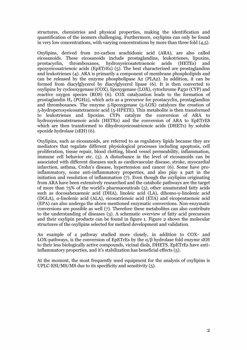
Since the early 90s it has been possible to identify endogenous mammalian substances referred to as endocannabinoids (EC), which bind to and activate cannabinoid receptors, e.g. CB1 and CB2, and are derived from membrane phospholipids (9,10). These receptors are known to mediate the psychotropic effects of marijuana (11). The CB1 receptor is found in abundance in the hippocampus, cortex, cerebellum and basal ganglia regions of the brain, while the CB2 receptor is mainly found in tissue of the immune system (12). Both receptors can also be found in the reproductive system (13). The first endocannabinoid discovered was anandamide (arachidonoyl ethanolamide, AEA), which was found in porcine brain in 1992 (10). Then followed the discovery of 2-arachidonoyl glycerol (2-AG), virodhamine (O-arachidonoyl ethanolamide, O-AEA), 2-arachidonoyl glycerol ether (noladin ether, 2-AGe) and N-arachidonoyl dopamide (NADA). 2-AG can rapidly isomerize to 1-AG, which does not act on CB receptors, but does occur physiologically (11,14). Later, docosatetraenoyl ethanolamide (DEA), docosahexaenoyl ethanolamide (DHEA) and eicosapentaenoyl ethanolamide (EPEA) were also reported as endocannabinoids acting on the CB1 and CB2 receptors (11,15). Structures of ECs acting on CB1 and CB2 receptors can be found in figure 3A. In addition to being an agonist at the cannabinoid receptors, ECs may also be able to act on receptors such as ion-channel transient receptor potential vanilloid type 1 (TRPV1) and orphan G-coupled receptors GPR55 (14). Besides the discovery of the above mentioned endocannabinoids, compounds structurally related to NADA and AEA have also been found in biological samples (Figure 3B). These compounds are not capable to act on the CB1 or CB2 receptors but may increase the effect of the endocannabinoids by competing for hydrolysis by the membrane-bound fatty-acid amide hydrolase (FAAH) or have an affinity with receptors such as TRPV1 or other receptors, that have not been identified yet (14,16). These compounds include: N-arachidonyl glycine (NAGly), oleoyl ethanolamide (OEA), palmitoyl ethanolamide (PEA), palmitoleoyl ethanolamide (POEA), linoleic acid ethanol amide (LEA), 2-linoleoyl glycerol (2-LG) and stearoyl ethanolamide (SEA) (14,17). Chemically, these compounds can be considered amides, esters or ethers of fatty acids (11). The “original” 5 ECs are amides, esters or ethers of arachidonic acid (18). The fatty acid precursors are shown in figure 3C.

6

O

OOH

OH

2-AG

O

OH

OH

2-AGe

O

NHHO

AEA

DEA

O

NHHO N

H

O

O

NH

NADA

HO

HO

O-AEA

O

NHHO

EPEA DHEA

O

OH2N

HO

HCl·

A.

O

NHHO

LEA

O

NH

HO2C

NAGly

O

N

OEA

HHO

O

OOH

OH

2-LG

O

N

POEA

HHO

O

NHHO

PEA

SEA

O

NHHO

B.

OH

O

ARA (Arachidonic acid)

OH

O

OLA (Oleic acid) DTA (Docosatetraenoic acid)

OH

O

OH

O

DHA (Docosahexenoic acid)

OH

O

EPA (Eicosapentaenoic acid)

OH

O

LA (Linoleic acid)

OH

O

POA (Palmitoleic acid)

OH

O

PA (Palmitic acid)

C.

Figure 3. Structures of ECs acting on CB1 and CB2 receptors (A) and of compounds structurally related to ECs without acting on CB1 and CB2 receptors but having the capability to increase the effect of ECs (B). Fatty acid precursors are shown in (C). Full names of the endocannbinoids can be found in the list of abbreviations.

7

The basal endocannabinoid concentrations in peripheral fluids such as plasma of healthy human subjects are on the threshold of the pM/nM range (14). Apart from being discovered in plasma, endocannabinoids have also been found in human brain tissue, human cerebrospinal fluid, rat brain, liver tissue, heart tissue and human bronchoalveolar lavage fluid (14). It is believed that the endocannabinoids and their related structures are biosynthesized “on demand” in different tissues from the postsynaptic neurons following physiological and pathological stimuli by depolarizing agents, hormones and neurotransmitters and are not stored in vesicles (12,14,18,19). They are also considered to be unstable and therefore rapidly metabolized by the intracellular membrane-bound enzyme FAAH and by monoacylglycerol lipases (MAGLs). FAAH degrades AEA to arachidonic acid and ethanolamine, while MAGL hydrolyzes 2-AG to arachidonic acid and glycerol (14,20). Much research on the so-called endocannabinoid system has been done in the last years and a significant amount of evidence reveals that the endocannabinoid system plays an important role in many physiological processes such as stress and anxiety, depression, inflammation, anorexia and bulimia, schizophrenia disorders, drug addiction, cardiovascular diseases, cancer, neurological disorders, fertility and reproduction, obesity and the metabolic syndrome (9,11,18). It has been realized that the endocannabinoid system may prove to be an efficient way to treat a wide variety of medical conditions (10). Furthermore, endocannabinoids might be potential biomarkers to determine target engagement for FAAH inhibition by novel pharmaceutical agents. Through FAAH inhibitors, endocannabinoid concentration increases and it is therefore being explored if these inhibitors can be novel treatment methods for diseases such as obesity and neuropathic pain (19). The best researched and most often quantified ECs are AEA and 2-AG. A number of GC-MS or LC-MS based methods for quantifying ECs, in particular AEA and 2-AG, and related structures have previously been reported (9,11,12,13,16,18,19). However LC-MS/MS is the most commonly used analytical technique for reasons of superior sensitivity and specificity (14).

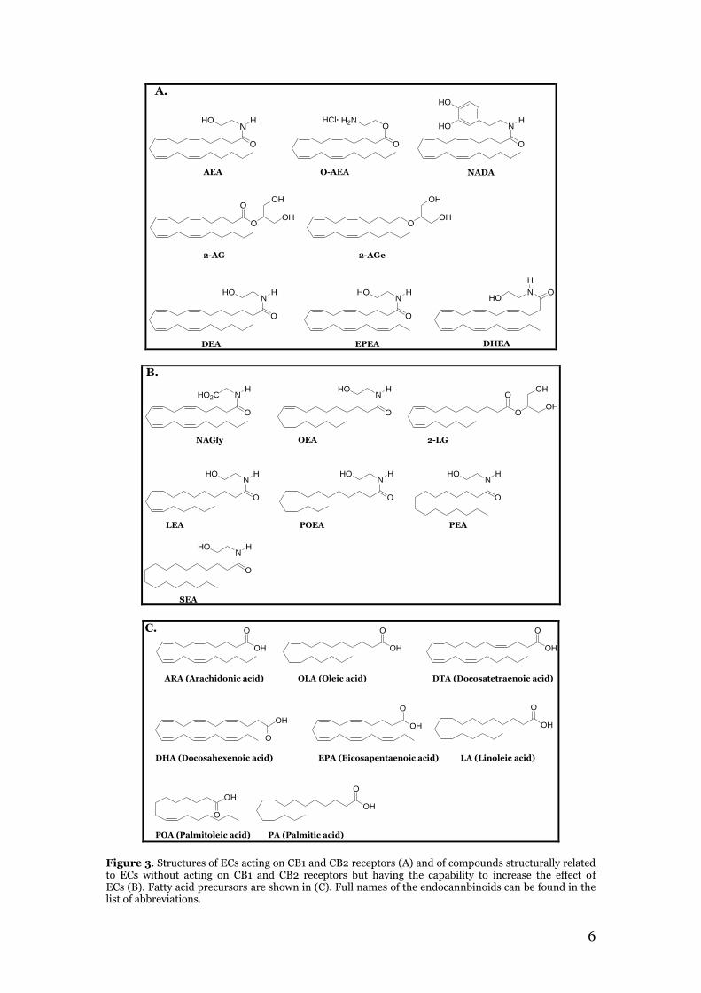
1.3 Instrumentation For the quantitative analysis of bioactive lipids, samples go through the process of preparation, analyte separation, analyte detection, and analyte quantification (figure 4).

Figure 4. Overview of the analytical workflow which was used for endocannabinoid analysis of samples from two human exposure studies. The internal standard (IS) was used for quantification purposes and the recovery standard (RS) in order to determine if the method performs well and to account for changes in volume and instrument variability.

8

1.3.1 Solid phase extraction

Solid phase extraction (SPE) is a frequently applied sample preparation technique used to enrich and separate analytes from other substances causing matrix effects before further analysis. There are four critical steps of the SPE procedure: conditioning of the SPE cartridges, loading of the sample, washing of the solid phase matrix while retaining the desired analytes and finally eluting the desired analytes from cartridges with appropriate solvents. The choice of solid phase sorbent material, washing and eluting solvent is based on the physical and chemical properties of the analytes to be studied. Hydrophobic-Lipophilic Balance (HLB) cartridges, as used in the experiments carried out during the diploma work, are cartridges containing a universal polymeric reversed-phase sorbent. These can be used for the extraction of a broad range of acidic, basic, and neutral analytes. Depending on the analytes, normal phase and ion exchange sorbents can also be considered for SPE (21,22).

1.3.2 Ultra-performance liquid chromatography (UPLC)

UPLC is an analytical technique to separate components in a mixture for purification, identification and quantification purposes (23,24). Components in a liquid sample or in a solid sample diluted in an appropriate solvent are passed through a column packed with silica-based particles (stationary phase) by pumping a solvent (mobile phase) through the column. Depending on the component’s chemical nature, size and on the interactions of the component with the mobile and stationary phase, the components are carried through the column at different speeds and reach the end of the column at different times (retention times), thus enabling a separation of the compounds in the mixture. The higher the affinity to the column, the slower the compounds migrate. The higher the affinity to the mobile phase, the faster the compounds elute from the column. The most commonly used LC system is reversed phase chromatography, in which the stationary phase is non-polar and the mobile phase polar. The stationary phase is most often an organochlorosilane for which the R group is a n-octyl (C8) or n-octyldecyl (C18) hydrocarbon. Another system is normal-phase chromatography in which the stationary phase is polar and the mobile phase non-polar. Mobile phases are either delivered isocratically or via a gradient. When eluting with a gradient, the mobile phase composition changes during the separation run (23,25). By further reducing the particle size and enabling higher pressures, shorter analysis times, better resolution and sensitivity can be achieved which ultimately leads to less solvent consumption, which is the idea behind UPLC. UPLC has proven to have many advantages over other LC techniques, thus becoming increasingly popular (23,24).

1.3.3 Mass spectrometry (MS)

When the compounds reach the end of the chromatographic column, they enter the mass spectrometer, where the solvent is evaporated and the compounds ionized to obtain positive or negative charges. A mass spectrometer consists of three main parts: the ionization source, the mass analyzer and the detector (26,27). After being ionized in the ionization source, the ions are transferred to the mass analyzer which separates the sample compounds according to mass-over-charge ratio (m/z) of the ions. The ions then hit the detector which creates a mass spectrum. This spectrum graphically displays the signals showing the relative abundance of the signals depending on their m/z ratio (28). There are several ionization techniques possible in the ionization source. The most commonly used ionization technique for LC-MS is electrospray ionization (ESI). At

9

atmospheric pressure, the LC eluent is pumped through a needle into the ionization source. A high voltage of 3 or 4 kV is applied to the tip of the needle which results in a strong electric field turning the sample into an aerosol of highly charged droplets. The electrostatic field further dissociates the analyte molecules and the heated drying gas, usually nitrogen, removes the solvent from the droplets, causing the droplets to shrink. Eventually, charged sample ions, free from solvent, leave the droplets and pass through to the mass analyzer (29,30). ESI can be run in either positive or negative mode resulting in protonated molecular ions (M+H)+ in positive ionisation mode, and in deprotonated molecular ions (M-H)- in negative ionisation mode (30). There are several types of mass analyzers available on the market, of which quadrupoles and time of flight are currently the most frequently used. Tandem mass spectrometers (MS/MS) are mass spectrometers containing more than one analyzer and thus are able to offer further information about specific ions. A triple quadrupole is a mass analyzer consisting of three quadrupoles, Q1, Q2 and Q3. A quadrupole contains 4 rods which are applied with direct current (DC) and radio frequency (RF) voltages. Quadrupoles Q1 and Q3 work as mass filters, while Q2 serves as a collision cell. Multiple reaction monitoring (MRM) is the most commonly used mode for quantitative analysis with triple quadrupoles. The first quadrupole filters a certain precursor ion, not letting other ions pass. In the collision cell, a characteristic product ion is generated by collision of the precursor ion with a collision gas, for instance argon. The produced product ions are introduced into the third quadrupole where only a certain m/z can pass through. Other ions are filtered out. The MRM mode serves as a double mass filter, with the benefit of lowering noise and increasing selectivity. In MS/MS operation, other scan modes can also be run to obtain conclusive information about the sample (31).

1.3.4 Quantification by the internal standard method and recovery calculations

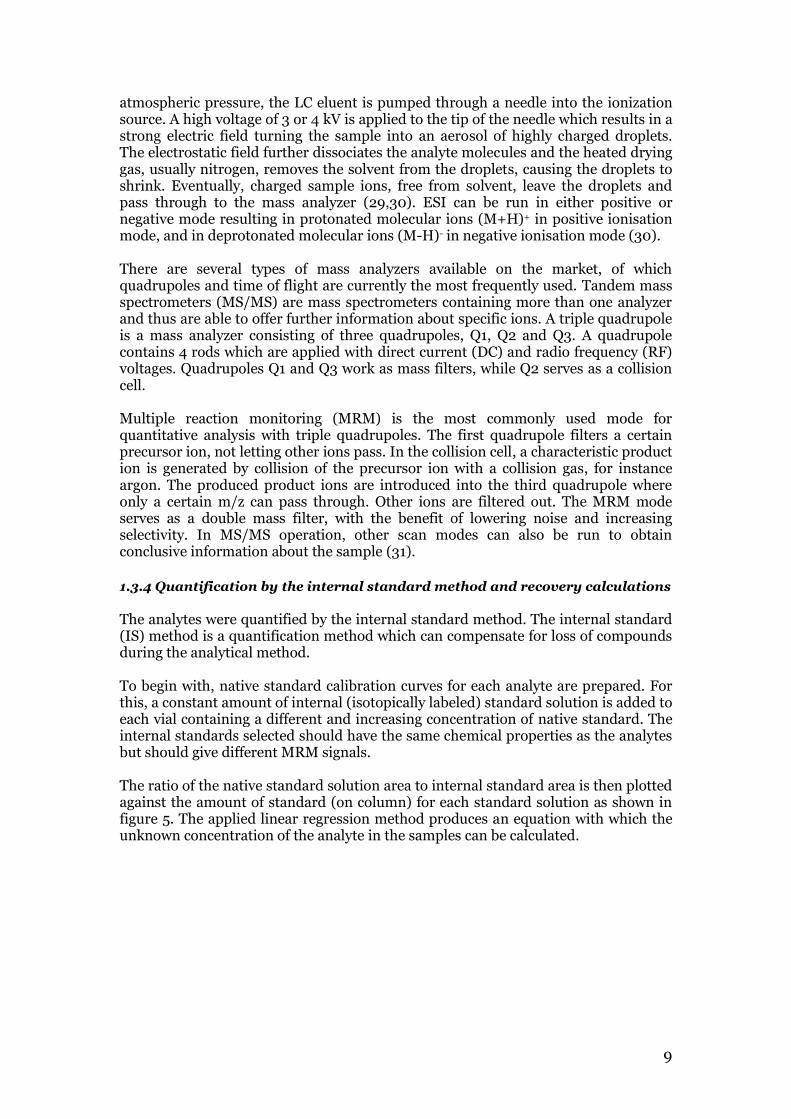
The analytes were quantified by the internal standard method. The internal standard (IS) method is a quantification method which can compensate for loss of compounds during the analytical method. To begin with, native standard calibration curves for each analyte are prepared. For this, a constant amount of internal (isotopically labeled) standard solution is added to each vial containing a different and increasing concentration of native standard. The internal standards selected should have the same chemical properties as the analytes but should give different MRM signals. The ratio of the native standard solution area to internal standard area is then plotted against the amount of standard (on column) for each standard solution as shown in figure 5. The applied linear regression method produces an equation with which the unknown concentration of the analyte in the samples can be calculated.

10

Figure 5. An example of a standard calibration curve with 8 samples. To create a linear regression trendline through the points, the least square method is applied. The linear regression equation y = mx

is shown in the lower right corner where m is the slope of the trendline. R2 is goodness of fit.

The samples undergo sample preparation via SPE. Before loading the sample to the SPE cartridges, the same amount of internal standard solution as added to the standard vials for standard curve preparation, is loaded onto the cartridges. The ratios of the area of the analyte in the sample to the internal standard area in the samples are calculated after sample peak selection and integration. For each analyzed compound, a standard calibration curve (see example in figure 5) had been prepared in advance. The linear regression equation generated through the least square method is used for calculating the unknown amount of analyte in each sample. The y value is the ratio of standard area to internal standard area (ratio AStd/AIS) while x is the unknown amount. The equation is solved for x which gives the unknown amount of the analyte in vial. Sample concentration is obtained after back-calculation to account for sample volume. Recovery calculations are carried out to show if the method has performed well. A calibration curve of the ratio between internal standard area and recovery standard area is prepared so that the loss of compounds during the application of the method can be calculated. The recovery is determined by calculating the amount of IS detected, after the analytical procedure, compared to the amount of internal standard added to the sample. The areas of internal standards and recovery standard are calculated in each sample and the ratio is used to determine the amount measured of the internal standard by solving the equation of the appropriate internal standard calibration curve for x. The recovery is usually reported as the fraction of IS left after extraction and should be between 25% and 150%. However, a recovery of >50-100% is preferred.

11

1.4 Developing and validating an UPLC-MS/MS method The goal of any analytical measurement is to attain reliable, precise and accurate data. In order to achieve this goal, it is important to validate an analytical method before applying it further to prove that the method is acceptable for its intended use. With the results from method validation, it is possible to judge the quality, reliability and consistency of analytical results. A validation process needs to occur before the first use of a method in routine testing, when slight method parameters have changed or when a new equipment is used for the method. Several organizations such as the Food and Drug administration (FDA) or the International Conference for Harmonization (ICH) and quality standards e.g. ISO17025 have created or listed guidelines for method validation but not any specific regulations (32). Yang et al. (4) validated a method developed for the analysis of oxylipins by determining linearity, limit of quantification (LOQ), accuracy, precision and recovery. Linearity of an analytical method is considered as its ability (within a given range) to receive test results that are directly proportional to the concentration of analyte in the sample (32). Linearity can be shown by injecting 5 to 6 standard solutions at different concentration levels spanning 80-120% of the targeted concentrantion range. By plotting the responses obtained against the concentrations and determining the correlation coefficient R2 after linear regression, conclusions on linear behavior can be drawn. The closer the correlation coefficient is to 1, the more linear behavior can be observed. The LOQ of an analytical process is defined as the lowest amount of analyte in a sample which can be quantitatively determined with suitable precision and accuracy (32). The LOQ is the amount of standard required to receive a signal to noise ratio of 10. Limit of detection (LOD) is on the other hand the amount of standard needed to obtain a signal to noise ratio of 3 (33). The accuracy of an analytical procedure is the closeness of the value measured to the true value. The mean value of accuracy should lie within 20% of the actual value (34). The precision is considered as the amount of scatter in the results received from a series of analyses of one homogenous sample. The precision calculated as the relative standard deviation at each concentration level should not exceed 15% (34). In order to determine the recovery of an analyte in a certain matrix, the matrix is spiked with a specific amount of analyte and the amount recovered after extraction and analysis is determined (4). When developing an optimal LC-MS/MS method for the analysis of bioactive lipids, several challenges have to be taken into consideration. Bioactive lipids, in particular isomers and those with the same transitions, tend to be very similar in structure making it necessary to achieve an excellent chromatographic separation. In addition, the endogenous concentrations of bioactive lipids are very low and therefore, thourough optimization at each step of the method is needed to reach the best detection limit. It is also necessary to optimize the gradient and ion transitions in order to attain a high throughput method with a short run time. The instability of several compounds and the complexity of some matrices must also be taken into account when developing the method (4).

12

1.5 Multivariate data analysis Multivariate data analysis deals with the analysis and interpretation of complex data by presenting the results in easily interpretable plots which are based on mathematical projection. Multivariate projection methods such as principal component analysis (PCA), partial least squares projections to latent squares (PLS) and orthogonal-PLS (O-PLS) have been successfully implemented in a broad range of application fields for modelling and interpreting complex data structures. PCA is usally the first step when analyzing the data and provides an overview of the dataset. It can easily recognize outliers, trends, groupings etc. Partial least squares projections to latent squares (PLS) is used to find a relationship between an input and output variable. O-PLS is a modification of PLS aimed at improving the interpretation of the resulting models (35).

1.6 Acrolein exposure study As the presence of chemicals in the environment, in food and consumer goods has increased in industrialized countries in the last decades, so have chemical related diseases/conditions including multiple chemical sensitivity, sick building syndrome, asthma and various cancers. More than ever are we exposed to man-made chemicals in food packaging materials, air pollution, electronics, toys, buildings, vehicles; making it almost inevitable to avoid chemicals in our daily life (36,37). Levels which are considered safe and not noticeable to most of us can provoke a number of non-specific symptoms for chemical sensitive persons including nausea, congestion, itching, sneezing, sore throat, headaches, skin rash etc. (38,39). Due to the wide variety of symptoms that can occur, it is often difficult for physicians to identify the sickness and relate it to chemical exposure. Chemical related illnesses are also considered to be controversial because many experts and physicians often do not have enough evidence to connect the patient’s symptoms and environmental exposure with each other (38). Therefore, patients suffering from these symptoms often feel misunderstood and are subject to ignorance leading to a new and growing health problem, which many physicians are still not trained to treat properly (39). Given that there is no cure for patients suffering from any of these conditions, these people can hardly lead a normal life, often being forced to reduce their working hours, leave their job or move away. This affects their quality of life and can even lead to social isolation due to this permanent disability (40). Women seem to suffer more likely from chemical-related illnesses than men (38). The main purpose of this exposure study, which was conducted at the Department of Psychology, Umeå University, Sweden, was to distinguish differences between healthy subjects and subjects sensible to chemicals when exposed to a sub-threshold concentration of acrolein, a reactive aldehyde, which is an irritant with a sharp, foul-smelling odor. Acrolein irritates eyes and mucous membranes and also the upper respiratory tract (41,42). Acrolein is structurally related to formaldehyde and shows similar effects. Most of the acrolein found in our environment arises from fossil fuel emissions from industrial and vehicle sources and acrolein is known to be a by-product of combustion and is found in high concentrations in urban areas (41). Furthemore, it is also produced during cooking and is a component of tobacco smoke. At room temperature, acrolein is a liquid but it is volatile so that you are mostly exposed to it through inhalation. Even though acrolein is able to cause death at rather low air

13

concentrations, overexposure is not likely due to its horrific smell. The potential of acrolein to cause cancer is not yet clarified but suspected (42). As a sub-study of the main exposure study, endocannabinoids in the exposed subjects’ plasma were quantified at the Department of Chemistry, Umeå University, Sweden. Blood samples and results obtained from the subjects after assessing their perceived exertion using the Borgs scale were collected which were then used for analysis of different outcomes. The subjects were recruited through an advertisement in a local newspaper. Each subject received a total of 600 SEK (100 SEK for each blood sample). The study was ethically approved by the Umeå Regional Ethics Board and performed in congruence with the Helsinki Declaration. The study was carried out in the Department of Psychology in January and February of 2013 and was led by principal investigator Anna-Sara Claesson, Assistant Professor at the Department of Psychology.

1.7 Biodiesel exhaust exposure study Urban air pollution causes approximately 1.3 millions deaths worldwide per year (43). There is considerable evidence that diesel emissions, as a contributor of air pollution, pose serious risks on human health which can lead to premature death. Petroleum diesel exhaust is made up of several hundreds of compounds, either in particulate or gaseous form. The different components can vary depending on fuel source, engine type, engine load and level of equipment maintenance, however evidence has shown that most are toxic or even carcinogen. Air toxics include benzene, 1,3-butadiene and formaldehyde. The soot is normally less than 2.5 µm in diameter making it possible for the particles to enter the peripheral lung regions and to interfere with gas exchange inside the lungs (43,44). Soot at this size has been associated to a number of negative health effects including lung inguries, asthma, allergic reactions, heart attacks, strokes, cancer and in general increasing mortality (45,46). Growing health problems, higher crude oil prices, decreasing resources of fossil oil and environmental concerns have led to a search for new fuel alternatives (44,47). Among these new alternatives, biodiesel made from plant oils (soybean, rapeseed and sunflower for example) has become increasingly popular and can be used in unmodified diesel engines with only a slight decrease in performance (44,48). Biodiesel is biodegradable, significantly less toxic to aquatic organisms (in the case of spills) than petroleum diesel and can be produced from renewable sources (44). In comparison to petroleum diesel exhaust, biodiesel emissions have also shown to consist of less particulate matter, carbon monoxide and polycyclic aromatic hydrocarbons (PAHs). Compounds containing sulfur seem to have dissapeared completely. However, there is an increase of nitrogen oxides when using biodiesel in an engine. Nitrogen oxides, in addition to contributing to health problems, have also been shown to induce the production of ozone. When using 100% biodiesel instead of petroleum diesel, the soluble organic fraction of the particles increases by approximately 40% whereas less insoluble organic mass is emitted (49). This variation in the fractions may also have an effect on the toxicity of biodiesel particles (48). While there is considerable evidence on the negative health effects of petroleum diesel exhaust, there have been limited studies on the effects of biodiesel exhaust on human health and the local environment (44,48). At present, there has only been an animal study performed that showed increased cardiovascular, pulmonary and inflammatory responses in mice when exposed to biodiesel exhaust (51). Most

14

biodiesel studies have set their focus on the analysis of exhaust emission material, motor efficiency, and on different methods for producing biodiesel but under laboratory conditions and not in biological systems (48,50,52). The biodiesel exhaust exposure study was conducted at the Department of Public Health and Clinical Medicine, Division of Respiratory Medicine and Allergy, at Norrlands University Hospital, Umeå, Sweden (in collaboration with the Center for Cardiovascular Science, University of Edinburgh, Edinburgh, UK) to investigate the effects of biodiesel exhaust on human health. As a sub-study of the main exposure study, endocannabinoids in the exposed subjects’ plasma were quantified at the Department of Chemistry, Umeå University, Sweden. The endocannabinoids analyzed in the plasma samples are one of many endpoints investigated. To detect cardiovascular responses, a venous occlusion plethysmography was performed and pulse and blood pressure were measured. A venous occlusion plethysmography is considered to be the epitome of methods when evaluating vascular endothelial function (51). For respiratory inflammation responses, nitric oxide levels were measured and collection of particles in exhaled air, a non-invasive sampling technique, was performed. Urine was taken to test for oxidative stress and other biomarkers. Blood samples were used to detect inflammatory markers, thrombosis, to perform a complete blood count, and for metabolomics analysis (oxylipins, endocannabinoids etc.). Exhaled carbon monoxide levels were measured because biofuels give off more carbon monoxide than ordinary fuels. This was considered as a safety measurement since this was the first ever human exposure to biodiesel exhaust. A lung function test was also conducted, primarily for safety reasons (51). The subjects were recruited through an advertisement in a local newspaper. Each subject received a total of 3000 SEK. The study was ethically approved by the Umeå Regional Ethics Board and performed in congruence with the Helsinki Declaration. The exposures were carried out at SMP Svensk Maskinprovning AB, Umeå, Sweden, and led by MD, PhD Jenny Bosson and co-workers at the Norrlands University Hospital in collaboration with researchers at the University of Edinburgh.

15

2. Material and Methods

2.1 Chemicals The endocannabinoids AEA, 2-AG, O-AEA, 2-AGe, NADA, DHEA, EPEA, NAGly, OEA, PEA, LEA, SEA, POEA, 2-LG, DEA as well as the deuterated endocannabinoids AEA-d8, 2-AG-d8, OEA-d4 and DHEA-d4 were purchased from Cayman Chemical (Ann Arbor, MI, USA) in the amounts listed in table 1 in the appendix. The oxylipins TXB2, 8-iso-PGE2, 8-iso-PGF2α, PGE2, PGD2, 12,13-DiHOME, 12(S)-HEPE, 13-HODE, 9(S)-HODE, 15-HETE, 17-HDoHE, 9-oxo-ODE, 12-oxo-ETE, 12-HETE, 5-HETE and 12(13)-EpOME, CUDA as well as the deuterated oxylipins TXB2-d4, PGE2-d4, 12,13-DiHOME-d4, 9(S)-HODE-d4, 12(13)-EpOME-d4 were purchased from Cayman Chemical (Ann Arbor, MI, USA) in the amounts listed in table 2 in the appendix. HPLC grade methanol and acetonitrile was either purchased from Merck (Darmstadt, Germany) or Fisher Scientific (Loughborough, UK). Ethylacetate was purchased from Fisher Scientific (Loughborough, UK). Ammonium acetate was obtained from Scharlau Chemie (Barcelona, Spain). Glacial acetic acid was purchased from Aldrich Chemical Company, Inc. (Milwaukee, WI, USA). Analytical reagent grade glycerol was purchased from Fischer Scientific (Loughborough, UK). Phosphate buffered saline was purchased from Fluka Analytical, Sigma-Aldrich (Buchs, Switzerland). Waters Oasis HLB cartridges (60 mg sorbent, 30 µm particle size) were purchased from Waters, Sweden.

2.2 Method development for oxylipin quantification by LC/MS A method for analysis of 16 oxylipins in a single injection was developed using 5 internal standards. Some were supplied in ethanol, some in methylacetate. Others were supplied as a solid. For the standards supplied in methylacetate, the solvent was carefully evaporated under nitrogen stream and then redissolved in ethanol to make a stock solution. The final standard stock solution concentrations were determined based on previous research (refer to table A2 in the appendix). If the compound was easy to ionize, then a low concentration was sufficient. A standard mixture solution was prepared from all stock solutions in order to perform UPLC-ESI/MS/MS optimization. Briefly, 10 µL of each stock solution (standard and intenal standards) were added to a vial reaching a final concentration of 23.8 µg/mL for each oxylipin with a stock solution concentration of 1000 µg/mL, of 2.38 µg/mL for each oxylipin with a stock solution concentration of 100 µg/mL, and of 11.9 µg/mL for each oxylipin with a stock solution concentration of 500 µg/mL. 100 µL of this mixture was transferred to a LC vial, which was used for LC/MS optimization. The method was optimized with an UPLC (Waters Acquity UltraPerformance) coupled to a triple quadrupole mass spectrometer (Quattro Ultima Micromass). The liquid chromatographic separation was conducted on a Waters BEH C18 column (2.1 mm x 150 mm, 2.5 µm particle size). The MS instrument was operated in negative mode. Desolvation temperature was set to 400 °C. N2 was used as drying gas and Ar as nebulization gas. The autosampler temperature was kept at 10 °C and the column was maintained at either 60 °C or 40 °C. Flow rates of 0.2, 0.3 and 0.4 mL/min were tested. Different mobile phases and gradients were tested as well.

16

After optimization of the LC system, MS parameters were also optimized. The standard/internal standard mixture solution was used to collect data in MS full scan run in negative mode. The scan range was 100 < m/z < 600. By using the MS full scan mode, it was possible to identify the [M-H]- ions to see if all standards and internal standards were detected. The amount injected was 2 µL. A fragmentation experiment of the [M-H]- ions was performed to identify the transitions of these ions, determined by the highest intensity peaks, which were possible transitions for quantifying the compounds. These transitions were then used in the MRM experiments. The MRM was split into two parts: 1) 0-14 minutes and 2) 11-21 minutes in order to increase the sensitivity. The transitions with the highest intensity were used as quantification and qualification ions, the transitions with lower intensity only as qualification ions. For both transitions, the optimum CAP (capillary voltage), CE (collision energy), and CV (cone voltage) were determined, by testing CV ranging from 100 to 4000 V, CEs from 8 to 70 eV and CVs from 15 to 40 V. After integration of the peaks, the highest obtained areas defined the optimum settings for each compound.

2.3 Oxylipin method validation Linearity, LOQ, recovery, inter- and intraday accuracy and precision were determined for the method.

2.3.1 Linearity and LOQ

The linearity of the method was determined by the calibration curves of each compound. A certain volume of each standard stock solution was used to obtain the strongest working solution (S1, shown in table A3 in the appendix). This solution was then diluted with methanol in several steps. The dilutions to obtain the calibration curves are shown in table A4 and A5 in the appendix. The calibration solutions for measurement in the UPLC-ESI/MS/MS system were prepared by adding 90 µL Sn solution, 10 µL recovery standard CUDA and 10 µL IS2 (4 µg/mL) to LC vials. The ratio of the areas of the native standards and the areas of the corresponding internal standards were plotted against the amount of compound (ng on column). The calibration curves were calculated by linear regression. By measuring the standard solutions at different, and decreasing, concentrations, it was possible to determine the LOQ of the compounds. For some compounds it was necessary to dilute the weakest standard solution S11 to obtain the final LOQ value.

2.3.2 Recovery for SPE extraction

Method recovery determines the amount of analyte spiked in the matrix that can be recovered and quantified (4). Phosphate buffer saline (PBS) solutions and plasma samples were spiked with 10 µL of three different internal standard solutions and 10 µL of antioxidant solution BHT/EDTA and extracted by SPE. The antioxidant solution was prepared by dissolving 0.4 mg BHT into 1 mL MeOH and 0.4 mg EDTA into 1 mL H2O and mixing the two solutions with MeOH:H2O (1:1, v/v). The SPE cartridges were washed with 2 column volumes (CV) of washing solution (95% H2O, 5% MeOH, 0.1% acetic acid). The compounds were extracted with 1 mL MeOH and 2 mL ethylacetate into tubes containing 6 µL of 30% glycerol in methanol as trap solution. The samples were then dried in the Speedvac until only glycerol remained. After adding 100 µL of MeOH , the tubes were vortexed. The

17

solutions were transferred to a LC vial and 10 µL of recovery standard (CUDA) was added, followed by measurement in the UPLC-ESI/MS/MS system. In order to determine the amount measured of the internal standards, a calibration curve was created by measuring 5 different concentrations of an internal standard solution in the UPLC-ESI/MS/MS and plotting the ratio of the areas of the internal standard area and the recovery standard against the amount of compound on column. The calibration curves were then determined by linear regression.

2.3.3 Inter- and intraday precision and accuracy

Accuracy and precision of the method were determined with the help of 4 quality control (QC) samples. QC prepared at different concentrations and that covered the whole linear concentration range. QCn (n=1-4) were prepared with 10 µL ISn + 90 µL PBS (100 mM) + 10 µL CUDA (800 nM). To determine the method’s intraday precision and accuracy, three injections were run daily (n=3). To determine the method’s interday precision and accuracy, QC samples were measured on three different days (n=9).

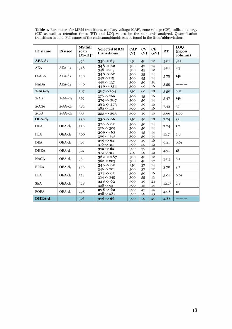
2.4 Endocannabinoid quantification The samples were analyzed with an UPLC (Waters Acquity UltraPerformance) coupled to a triple quadrupole mass spectrometer (Quattro Ultima Micromass). The liquid chromatographic separation was conducted on a Waters BEH C18 column (2.1 mm x 150 mm, 2.5 µm particle size). The autosampler temperature was kept at 10 °C and the column was maintained at 60 °C. Desolvation temperature was set to 400 °C. N2 was used as drying gas and Ar as nebulization gas. The mass spectrometer was operated in positive ESI mode. Endocannabinoids were separated using H2O with 10 mM CH3COONH4 (A) and MeOH with 10 mM CH3COONH4 (B) as mobile phases with a flow rate of 0.4 mL/min. The following gradient was applied: 0.0-9.0 min (79%B), 9-9.5 min (79-90%B), 9.5-10.5 min 90%B, 10.5-13.0 min 100%B, 13.0-15.0 min 100%B, 15.10-18.0 min 79%B. The injection volume for samples and standards was 10 µL. The method was previously developed and validated. MRM for all standards was performed with optimal transitions, which were determined by precursor ion experiments. A list of all instrument parameters can be found in table 1. All data was processed and analyzed using Masslynx software version 4.1.

18

Table 1. Parameters for MRM transitions, capillary voltage (CAP), cone voltage (CV), collision energy (CE) as well as retention times (RT) and LOQ values for the standards analyzed. Quantification transitions in bold. Full names of the endocannabinoids can be found in the list of abbreviations.

EC name IS used MS full scan [M+H]+

Selected MRM transitions

CAP (V)

CV (V)

CE (eV)

RT LOQ (pg on column)

AEA-d8 356 356 -> 63 250 40 12 5.01 341

AEA AEA-d8 348 348 -> 62 348 ->203

500 500

42 45

14 12

5.01 7.3

O-AEA AEA-d8 348 348 -> 62 348 ->215

500 500

35 45

14 14

5.75 146

NADA AEA-d8 440 440 -> 137 440 -> 154

500 500

50 60

28 16

5.55 ---------

2-AG-d8 387 387 ->294 250 60 18 5.50 682

2-AG 2-AG-d8 379 379 -> 269 379 -> 287

500 500

45 50

16 14

5.47 146

2-AGe 2-AG-d8 382 382 -> 273 382 -> 121

500 500

30 30

10 16

7.42 37

2-LG 2-AG-d8 355 355 -> 263 500 40 10 5.66 1170

OEA-d4 330 330 -> 66 250 40 18 7.24 32

OEA OEA-d4 326 326 -> 62 326 -> 309

500 500

50 50

14 14

7.24 1.2

PEA OEA-d4 300 300 -> 62 300 -> 283

500 500

45 50

14 14

12.7 2.8

DEA OEA-d4 376 376 -> 62 376 -> 315

500 500

40 55

16 12

6.21 0.61

DHEA OEA-d4 372 372 -> 62 372 -> 311

500 250

35 50

16 10

4.91 18

NAGly OEA-d4 362 362 -> 287 362 -> 203

500 500

40 40

12 17

3.05 6.1

EPEA OEA-d4 346 346 -> 62 346 -> 201

250 500

37 37

14 12

3.70 3.7

LEA OEA-d4 324 324 -> 62 324 -> 245

500 500

50 55

16 12

5.01 0.61

SEA OEA-d4 328 328 -> 62 328 -> 62

500 500

40 45

24 14

12.75 2.8

POEA OEA-d4 298 298 -> 62 298 -> 281

500 500

47 50

14 13

4.08 12

DHEA-d4 376 376 -> 66 500 50 20 4.88 ---------

19

2.4.1 Standard stock solution preparation

The endocannabinoids were commercially supplied as listed in table A1 (see appendix). The solvent was dried under nitrogen for endocannabinoids supplied in methylacetate and residues were reconstituted in 100 µL of ethanol. A specific volume of ethanol was added to the endocannabinoids supplied as solids (table A1 in the appendix). For each standard, stock solutions were prepared. For the acrolein exposure experiments, stock solution concentrations of 250 µg/mL were prepared for AEA, 2-AG, 2-AGe, NADA, DHEA, EPEA, NAGly, OEA, LEA, POEA and DEA. For SEA, a final concentration of 83.3 µg/mL was prepared. For PEA, a final concentration of 251 µg/mL was prepared, and for 2-LG and O-AEA a final concentration of 154 µg/mL. For the biodiesel exhaust exposure experiment, a final stock concentration of 125 µg/mL was prepared for the following compounds: AEA, PEA; OEA, DEA, NAGly, EPEA and DHEA. O-AEA and 2-LG were prepared at a final stock solution of 250 µg/mL. The other concentrations remained the same. Stock solutions of IS AEA-d8, 2-AG-d8 and OEA-d4were prepared to receive a final concentration of 40 µg/mL. A stock solution of the recovery standard DHEA-d4 was prepared at 10 µg/mL. The preparation steps can be found in table A1 of the appendix. The stock solutions of the standards and IS were stored at -80 °C, the recovery standard stock solution at -20 °C.

2.4.2 Native standard curve preparation

Standard calibration curve solutions in methanol were prepared from stock solutions on each day of the UPLC-ESI/MS/MS measurements to quantify the levels of ECs in the plasma samples. The highest concentration of the standard curve was prepared by adding 100 µL of each standard stock solution to a final volume of 1500 µL (Standard mixture solution S1). The further dilution steps and concentrations are found in tables A6-A10 in the appendix. Standard solution S10 was the lowest point in the calibration curve. 90 µL of each calibration solution was spiked with 10 µL of recovery standard stock solution and with 10 µL of internal standard solution (IS3). For each solution, the peaks were integrated and the ratio of each standard area and the corresponding internal standard area was plotted against the amount of standard on column in ng. The amounts of compound on column in ng and the calculations are shown in table A11 in the appendix. The slope and correlation coefficient of each standard curve was determined by linear regression analysis. Intercept was set to 0. Table A12 and A13 in the appendix show the values for slope and correlation coefficient for the calibration curves used in the acrolein exposure and in the biodiesel exhaust exposure experiment.

2.4.3 Internal standard curve preparation

Internal standard curves were prepared in order to determine the recovery of the spiked internal standards in all samples. Either 100 µL or 50 µL of each of the three stock solution was added to a vial and 300 µL of MeOH was added to obtain a final volume of 500 µL. This solution was then further diluted making 5 different calibration points. The dilutions and concentrations are shown in table A14 and A15 in the appendix. The concentration of each compound in the vial was calculated and the amount in ng on column determined. The calculations are shown in table A16 and A17 in the appendix.

20

10 µL of each internal standard calibration solution was added to 90 µL of MeOH and spiked with 10 µL of recovery standard stock solution and measured in the UPLC-ESI/MS/MS. The peaks were integrated and the ratio of the deuterated standards area and recovery standard area was plotted against the amount of deuterated standard on column in ng in each solution. The slope and correlation coefficient of each internal standard curve was determined by linear regression analysis. The intercept was set to 0. Table A18 and A19 in the appendix show the values for slope and correlation coefficient for the calibration curves used in the acrolein exposure and in the biodiesel exhaust exposure experiment.

2.4.4 Sample preparation process for acrolein exposure and biodiesel exhaust

exposure experiments

The plasma samples were defrosted at room temperature and if necessary centrifuged, and then extracted by SPE.Waters Oasis HLB cartridges (60 mg sorbent, 30 µm particle size) were washed with 1 CV of ethylacetate, followed by 2 CV of MeOH and 2 CV of wash solution (30% MeOH). Plasma was spiked with 10 µL of IS3 and applied to the SPE column. The plasma applied depended on the amount supplied (500-900 µL). In pre-tests, different volumes of plasma were purified via SPE. The signal to noise ratio after UPLC-ESI/MS/MS analysis was calculated with the Mass Lynx software for all compounds and the optimal amount of plasma was determined. 750 µL of plasma was found to be the amount with a signal to noise ratio above 10 for all compounds. The higher the amount of plasma, the more noise was detected. 1 mL was still alright, but for more than 1 mL and less than 500 mL, the signal to noise ratio was not tolerable for the majority of compounds. After adding plasma to the columns, the columns were washed with 1 CV of wash solution (30% MeOH) and dried under high vacuum. The analytes were eluted into polypropylen tubes with 3 mL of ACN, followed by 1 mL of MeOH and 1 mL of ethylacetate. To completely remove the remaining solvents from the cartridges, high vacuum was applied for several minutes. 6 µL of 30% glycerol in MeOH served as a trap solution for the analytes which was therefore added to each tube following the extraction. The solvents were evaporated with a SpeedVAC system (Farmingdale, NY, USA) until approximately 2 µL of the trap solution was left. 100 µL of MeOH was added to each remaining solution and the solution was vortexed to dissolve any residues, and if necessary centrifuged. Afterwards, the solutions were transferred to LC vials with low volume inserts and 10 µL of recovery standard DHEA-d4 was added. 10 µL was then injected into the UPLC-ESI/MS/MS system for analysis.

21

2.5 Application of the UPLC-ESI/MS/MS method for quantification of endocannabionoids in human plasma The UPLC-ESI/MS/MS method for endocannabinoid quantification was applied to human plasma obtained from two different exposure studies.

2.5.1 Experimental design of the acrolein exposure study

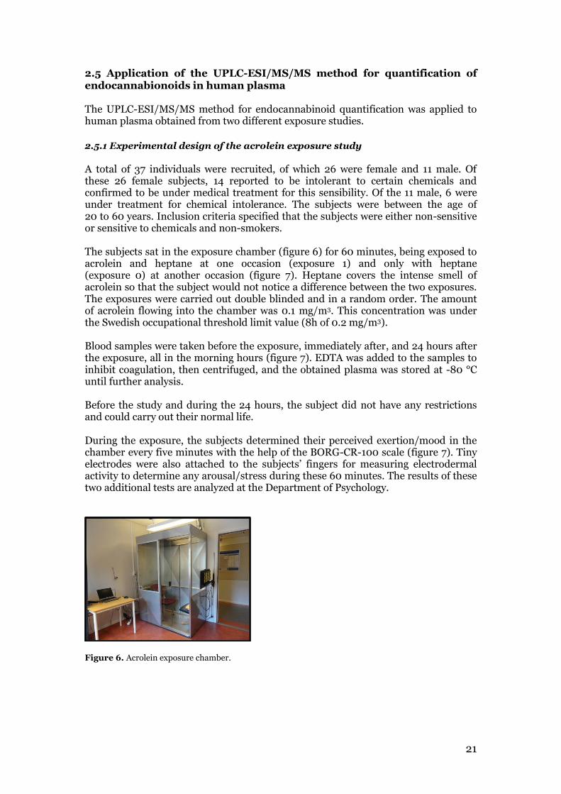
A total of 37 individuals were recruited, of which 26 were female and 11 male. Of these 26 female subjects, 14 reported to be intolerant to certain chemicals and confirmed to be under medical treatment for this sensibility. Of the 11 male, 6 were under treatment for chemical intolerance. The subjects were between the age of 20 to 60 years. Inclusion criteria specified that the subjects were either non-sensitive or sensitive to chemicals and non-smokers. The subjects sat in the exposure chamber (figure 6) for 60 minutes, being exposed to acrolein and heptane at one occasion (exposure 1) and only with heptane (exposure 0) at another occasion (figure 7). Heptane covers the intense smell of acrolein so that the subject would not notice a difference between the two exposures. The exposures were carried out double blinded and in a random order. The amount of acrolein flowing into the chamber was 0.1 mg/m3. This concentration was under the Swedish occupational threshold limit value (8h of 0.2 mg/m3). Blood samples were taken before the exposure, immediately after, and 24 hours after the exposure, all in the morning hours (figure 7). EDTA was added to the samples to inhibit coagulation, then centrifuged, and the obtained plasma was stored at -80 °C until further analysis. Before the study and during the 24 hours, the subject did not have any restrictions and could carry out their normal life. During the exposure, the subjects determined their perceived exertion/mood in the chamber every five minutes with the help of the BORG-CR-100 scale (figure 7). Tiny electrodes were also attached to the subjects’ fingers for measuring electrodermal activity to determine any arousal/stress during these 60 minutes. The results of these two additional tests are analyzed at the Department of Psychology.

Figure 6. Acrolein exposure chamber.

22

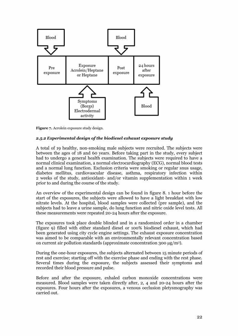
Figure 7. Acrolein exposure study design.

2.5.2 Experimental design of the biodiesel exhaust exposure study

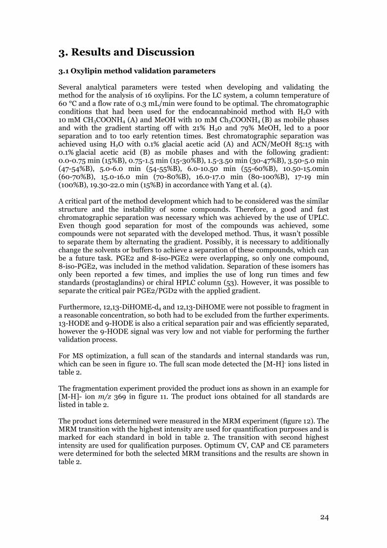
A total of 19 healthy, non-smoking male subjects were recruited. The subjects were between the ages of 18 and 60 years. Before taking part in the study, every subject had to undergo a general health examination. The subjects were required to have a normal clinical examination, a normal electrocardiography (ECG), normal blood tests and a normal lung function. Exclusion criteria were smoking or regular snus usage, diabetes mellitus, cardiovascular disease, asthma, respiratory infection within 2 weeks of the study, antioxidant- and/or vitamin supplementation within 1 week prior to and during the course of the study. An overview of the experimental design can be found in figure 8. 1 hour before the start of the exposures, the subjects were allowed to have a light breakfast with low nitrate levels. At the hospital, blood samples were collected (pre sample), and the subjects had to leave a urine sample, do lung function and nitric oxide level tests. All these measurements were repeated 20-24 hours after the exposure. The exposures took place double blinded and in a randomized order in a chamber (figure 9) filled with either standard diesel or 100% biodiesel exhaust, which had been generated using city cycle engine settings. The exhaust exposure concentration was aimed to be comparable with an environmentally relevant concentration based on current air pollution standards (approximate concentration 300 µg/m3). During the one-hour exposures, the subjects alternated between 15 minute periods of rest and exercise; starting off with the exercise phase and ending with the rest phase. Several times during the exposure, the subjects assessed their symptoms and recorded their blood pressure and pulse. Before and after the exposure, exhaled carbon monoxide concentrations were measured. Blood samples were taken directly after, 2, 4 and 20-24 hours after the exposures. Four hours after the exposures, a venous occlusion pletysmography was carried out.

23

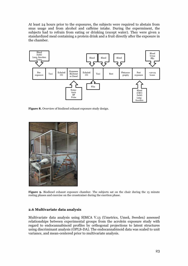
At least 24 hours prior to the exposures, the subjects were required to abstain from snus usage and from alcohol and caffeine intake. During the experminent, the subjects had to refrain from eating or drinking (except water). They were given a standardized meal containing a protein drink and a fruit directly after the exposure in the chamber.

Figure 8. Overview of biodiesel exhaust exposure study design.

Figure 9. Biodiesel exhaust exposure chamber. The subjects sat on the chair during the 15 minute resting phases and exercise on the crosstrainer during the exertion phase.

2.6 Multivariate data analysis Multivariate data analysis using SIMCA V.13 (Umetrics, Umeå, Sweden) assessed relationships between experimental groups from the acrolein exposure study with regard to endocannabinoid profiles by orthogonal projections to latent structures using discriminant analysis (OPLS-DA). The endocannabinoid data was scaled to unit variance, and mean-centered prior to multivariate analysis.

24

3. Results and Discussion

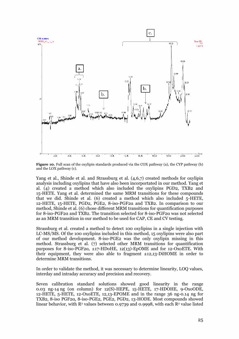
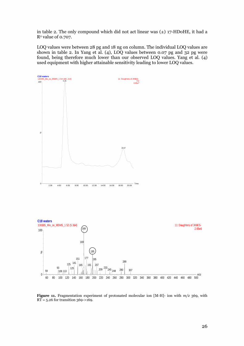
3.1 Oxylipin method validation parameters Several analytical parameters were tested when developing and validating the method for the analysis of 16 oxylipins. For the LC system, a column temperature of 60 °C and a flow rate of 0.3 mL/min were found to be optimal. The chromatographic conditions that had been used for the endocannabinoid method with H2O with 10 mM CH3COONH4 (A) and MeOH with 10 mM Ch3COONH4 (B) as mobile phases and with the gradient starting off with 21% H20 and 79% MeOH, led to a poor separation and to too early retention times. Best chromatographic separation was achieved using H2O with 0.1% glacial acetic acid (A) and ACN/MeOH 85:15 with 0.1% glacial acetic acid (B) as mobile phases and with the following gradient: 0.0-0.75 min (15%B), 0.75-1.5 min (15-30%B), 1.5-3.50 min (30-47%B), 3.50-5.0 min (47-54%B), 5.0-6.0 min (54-55%B), 6.0-10.50 min (55-60%B), 10.50-15.0min (60-70%B), 15.0-16.0 min (70-80%B), 16.0-17.0 min (80-100%B), 17-19 min (100%B), 19.30-22.0 min (15%B) in accordance with Yang et al. (4). A critical part of the method development which had to be considered was the similar structure and the instability of some compounds. Therefore, a good and fast chromatographic separation was necessary which was achieved by the use of UPLC. Even though good separation for most of the compounds was achieved, some compounds were not separated with the developed method. Thus, it wasn’t possible to separate them by alternating the gradient. Possibly, it is necessary to additionally change the solvents or buffers to achieve a separation of these compounds, which can be a future task. PGE2 and 8-iso-PGE2 were overlapping, so only one compound, 8-iso-PGE2, was included in the method validation. Separation of these isomers has only been reported a few times, and implies the use of long run times and few standards (prostaglandins) or chiral HPLC column (53). However, it was possible to separate the critical pair PGE2/PGD2 with the applied gradient. Furthermore, 12,13-DiHOME-d4 and 12,13-DiHOME were not possible to fragment in a reasonable concentration, so both had to be excluded from the further experiments. 13-HODE and 9-HODE is also a critical separation pair and was efficiently separated, however the 9-HODE signal was very low and not viable for performing the further validation process. For MS optimization, a full scan of the standards and internal standards was run, which can be seen in figure 10. The full scan mode detected the [M-H]- ions listed in table 2. The fragmentation experiment provided the product ions as shown in an example for [M-H]- ion m/z 369 in figure 11. The product ions obtained for all standards are listed in table 2. The product ions determined were measured in the MRM experiment (figure 12). The MRM transition with the highest intensity are used for quantification purposes and is marked for each standard in bold in table 2. The transition with second highest intensity are used for qualification purposes. Optimum CV, CAP and CE parameters were determined for both the selected MRM transitions and the results are shown in table 2.

25

Figure 10. Full scan of the oxylipin standards produced via the COX pathway (a), the CYP pathway (b) and the LOX pathway (c).

Yang et al., Shinde et al. and Strassburg et al. (4,6,7) created methods for oxylipin analysis including oxylipins that have also been incorportated in our method. Yang et al. (4) created a method which also included the oxylipins PGD2, TXB2 and 15-HETE. Yang et al. determined the same MRM transitions for these compounds that we did. Shinde et al. (6) created a method which also included 5-HETE, 12-HETE, 15-HETE, PGD2, PGE2, 8-iso-PGF2α and TXB2. In comparison to our method, Shinde et al. (6) chose different MRM transitions for quantification purposes for 8-iso-PGF2α and TXB2. The transition selected for 8-iso-PGF2α was not selected as an MRM transition in our method to be used for CAP, CE and CV testing. Strassburg et al. created a method to detect 100 oxylipins in a single injection with LC-MS/MS. Of the 100 oxylipins included in this method, 15 oxylipins were also part of our method development. 8-iso-PGE2 was the only oxylipin missing in this method. Strassburg et al. (7) selected other MRM transitions for quantification purposes for 8-iso-PGF2α, ±17-HDoHE, 12(13)-EpOME and for 12-OxoETE. With their equipment, they were also able to fragment ±12,13-DiHOME in order to determine MRM transitions. In order to validate the method, it was necessary to determine linearity, LOQ values, interday and intraday accuracy and precision and recovery. Seven calibration standard solutions showed good linearity in the range 0.03 ng-14 ng (on column) for 12(S)-HEPE, 15-HETE, 17-HDOHE, 9-OxoODE, 12-HETE, 5-HETE, 12-OxoETE, 12,13-EPOME and in the range 36 ng-0.14 ng for TXB2, 8-iso PGF2α, 8-iso-PGE2, PGE2, PGD2, 13-HODE. Most compounds showed linear behavior, with R2 values between 0.9739 and 0.9998, with each R2 value listed

26

in table 2. The only compound which did not act linear was (±) 17-HDoHE, it had a R2 value of 0.707. LOQ values were between 28 pg and 18 ng on column. The individual LOQ values are shown in table 2. In Yang et al. (4), LOQ values between 0.07 pg and 32 pg were found, being therefore much lower than our observed LOQ values. Yang et al. (4) used equipment with higher attainable sensitivity leading to lower LOQ values.

Figure 11. Fragmentation experiment of protonated molecular ion [M-H]- ion with m/z 369, with RT = 5.26 for transition 369->169.

C18 waters

Time2.00 4.00 6.00 8.00 10.00 12.00 14.00 16.00 18.00 20.00

%

0

100

130305_Mix_ox_MSMS_1 Sm (Mn, 2x3) 11: Daughters of 369ES- TIC

3.05e7

5.26

18.67

C18 waters

m/z60 80 100 120 140 160 180 200 220 240 260 280 300 320 340 360 380 400 420 440 460 480 500

%

0

100

130305_Mix_ox_MSMS_1 52 (5.364) 11: Daughters of 369ES- 2.65e6169

169

151

141125

9359 113109

125165

195

177

191

195289

207233

209 245 280248 307

27

05

10

15

0

20

00

0

40

00

0

60

00

0

80

00

0

TX

B2

-d4

(3

73

>1

73

)

tim

e /

min

intensity

rt 5

.04

min

05

10

15

0

10

00

00

20

00

00

30

00

00

40

00

00

50

00

00

TX

B2

(3

69

>1

69

)

tim

e /

min

intensity

rt 5

.04

min

05

10

15

0

20

00

0

40

00

0

60

00

0

PG

E2

-d4

(3

55

>2

75

)

tim

e /

min

intensity

rt 5

.33

min

05

10

15

0

50

00

00

10

00

00

0

15

00

00

0

20

00

00

0

25

00

00

0

8-i

so

PG

F2

(3

53

>3

09

)

tim

e /

min

intensity

rt 4

.86

min

05

10

15

0

10

00

00

20

00

00

30

00

00

40

00

008

-is

o-P

GE

2/

PG

E2

(3

51

>2

71

)

tim

e /

min

intensity

rt 5

.27

min

05

10

15

0

10

00

00

20

00

00

30

00

00

40

00

00

PG

D2

(3

51

>2

71

)

tim

e /

min

intensity

rt 5

.5.5

1 m

in

05

10

15

0

20

00

0

40

00

0

60

00

0

80

00

0

9(S

)-H

OD

E-d

4 (

29

9>

28

1)

tim

e /

min

intensity

rt 1

1.8

5 m

in

05

10

15

20

25

0

50

00

10

00

0

15

00

0

20

00

0

25

00

0

12

(S)-

HE

PE

(3

17

>1

79

)

tim

e /

min

intensity

rt 1

3.6

7 m

in

05

10

15

20

25

0

20

00

00

40

00

00

60

00

00

80

00

00

10

00

00

0

(+-)

13

-HO

DE

(2

95

>1

95

)

tim

e /

min

intensity

rt 1

1.6

8 m

in

05

10

15

20

25

0

10

00

00

20

00

00

30

00

00

40

00

00

(+-)

15

-HE

TE

(3

19

>2

19

)

tim

e /

min

intensity

rt 1

2.3

2 m

in

05

10

15

20

25

0

20

00

0

40

00

0

60

00

0

(+-)

17

-HD

oH

E (

34

3>

28

3)

tim

e /

min

intensity

rt 1

8.8

7 m

in

05

10

15

20

25

0

10

00

0

20

00

0

30

00

0

9-O

xo

OD

E (

29

3>

18

5)

tim

e /

min

intensity

rt 1

2.9

7 m

in

05

10

15

20

25

0

50

00

10

00

0

15

00

0

(+-)

12

-HE

TE

(3

19

>1

79

)

tim

e /

min

intensity

rt 1

3.1

8 m

in

05

10

15

20

25

0

50

00

0

10

00

00

15

00

00

(+-)

5-H

ET

E (

31

9>

11

5)

tim

e /

min

intensity

rt 1

4.1

3 m

in

05

10

15

20

25

0

50

00

0

10

00

00

15

00

00

20

00

00

12

-Ox

oE

TE

(3

17

>1

53

)

tim

e /

min

intensity

rt 1

3.6

1 m

in

05

10

15

20

25

0

50

00

10

00

0

15

00

0

20

00

0 12

(13

)-E

pO

ME

-d4

(2

99

>2

81

)

tim

e /

min

intensity

rt 1

4.2

7 m

in

05

10

15

20

25

0

50

00

00

10

00

00

0

15

00

00

0

20

00

00

0

12

(13

)-E

pO

ME

(2

95

>2

77

)

tim

e /

min

intensity

rt 1

4.3

7 m

in

Fig

ur

e 1

2.

MR

M d

iag

ram

s o

f th

e o

xy

lip

ins

incl

ud

ed

in

th

e m

eth

od

.

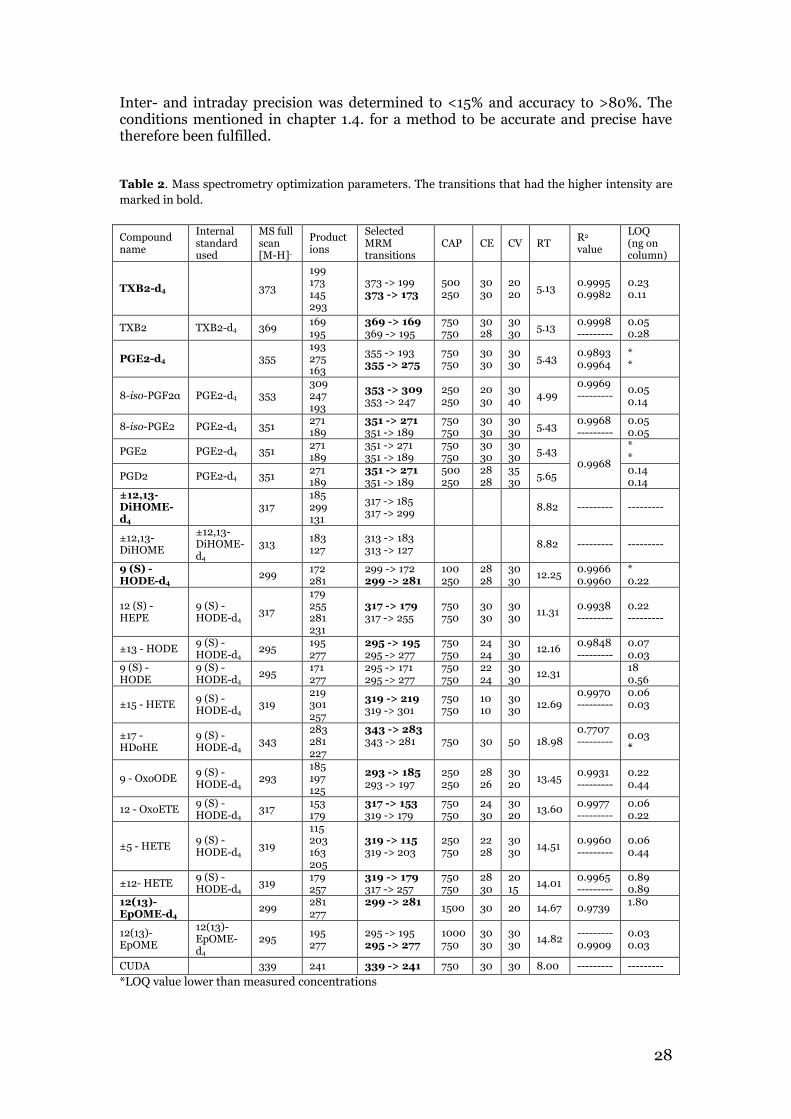
28

Inter- and intraday precision was determined to <15% and accuracy to >80%. The conditions mentioned in chapter 1.4. for a method to be accurate and precise have therefore been fulfilled. Table 2. Mass spectrometry optimization parameters. The transitions that had the higher intensity are

marked in bold.

Compound name

Internal standard used

MS full scan [M-H]-

Product ions

Selected MRM transitions

CAP CE CV RT R2

value

LOQ (ng on column)

TXB2-d4 373

199 173 145 293

373 -> 199 373 -> 173

500 250

30 30

20 20

5.13 0.9995 0.9982

0.23 0.11

TXB2 TXB2-d4 369 169 195

369 -> 169 369 -> 195

750 750

30 28

30 30

5.13 0.9998 ---------

0.05 0.28

PGE2-d4 355 193 275 163

355 -> 193 355 -> 275

750 750

30 30

30 30

5.43 0.9893 0.9964

* *

8-iso-PGF2α PGE2-d4 353 309 247 193

353 -> 309 353 -> 247

250 250

20 30

30 40

4.99 0.9969 ---------

0.05 0.14

8-iso-PGE2 PGE2-d4 351 271 189

351 -> 271 351 -> 189

750 750

30 30

30 30

5.43 0.9968 ---------

0.05 0.05

PGE2 PGE2-d4 351 271 189

351 -> 271 351 -> 189

750 750

30 30

30 30

5.43 0.9968

* *

PGD2 PGE2-d4 351 271 189

351 -> 271 351 -> 189

500 250

28 28

35 30

5.65 0.14 0.14

±12,13-DiHOME-d4

317 185 299 131

317 -> 185 317 -> 299

8.82 --------- ---------

±12,13-DiHOME

±12,13-DiHOME-d4

313 183 127

313 -> 183 313 -> 127

8.82 --------- ---------

9 (S) -HODE-d4

299 172 281

299 -> 172 299 -> 281

100 250

28 28

30 30

12.25 0.9966 0.9960

* 0.22

12 (S) - HEPE

9 (S) -HODE-d4

317

179 255 281 231

317 -> 179 317 -> 255

750 750

30 30

30 30

11.31 0.9938 ---------

0.22 ---------

±13 - HODE 9 (S) -HODE-d4

295 195 277

295 -> 195 295 -> 277

750 750

24 24

30 30

12.16 0.9848 ---------

0.07 0.03

9 (S) - HODE

9 (S) -HODE-d4

295 171 277

295 -> 171 295 -> 277

750 750

22 24

30 30

12.31 18 0.56

±15 - HETE 9 (S) -HODE-d4

319 219 301 257

319 -> 219 319 -> 301

750 750

10 10

30 30

12.69 0.9970 ---------

0.06 0.03

±17 - HDoHE

9 (S) -HODE-d4

343 283 281 227

343 -> 283 343 -> 281

750 30 50 18.98 0.7707 ---------

0.03 *

9 - OxoODE 9 (S) -HODE-d4

293 185 197 125

293 -> 185 293 -> 197

250 250

28 26

30 20

13.45 0.9931 ---------

0.22 0.44

12 - OxoETE 9 (S) -HODE-d4

317 153 179

317 -> 153 319 -> 179

750 750

24 30

30 20

13.60 0.9977 ---------

0.06 0.22

±5 - HETE 9 (S) -HODE-d4

319

115 203 163 205

319 -> 115 319 -> 203

250 750

22 28

30 30

14.51 0.9960 ---------

0.06 0.44

±12- HETE 9 (S) -HODE-d4

319 179 257

319 -> 179 317 -> 257

750 750

28 30

20 15

14.01 0.9965 ---------

0.89 0.89

12(13)-EpOME-d4

299 281 277

299 -> 281

1500 30 20 14.67 0.9739 1.80

12(13)-EpOME

12(13)-EpOME-d4

295 195 277

295 -> 195 295 -> 277

1000 750

30 30

30 30

14.82 --------- 0.9909

0.03 0.03

CUDA 339 241 339 -> 241 750 30 30 8.00 --------- ---------

*LOQ value lower than measured concentrations

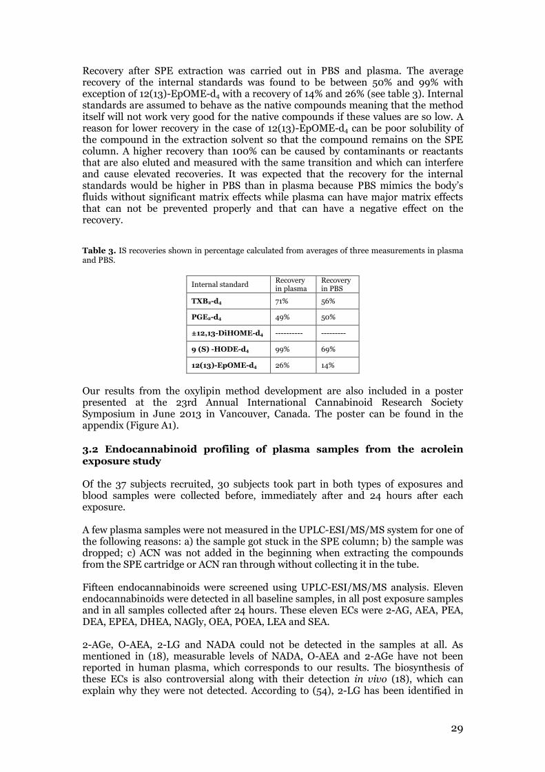
29

Recovery after SPE extraction was carried out in PBS and plasma. The average recovery of the internal standards was found to be between 50% and 99% with exception of 12(13)-EpOME-d4 with a recovery of 14% and 26% (see table 3). Internal standards are assumed to behave as the native compounds meaning that the method itself will not work very good for the native compounds if these values are so low. A reason for lower recovery in the case of 12(13)-EpOME-d4 can be poor solubility of the compound in the extraction solvent so that the compound remains on the SPE column. A higher recovery than 100% can be caused by contaminants or reactants that are also eluted and measured with the same transition and which can interfere and cause elevated recoveries. It was expected that the recovery for the internal standards would be higher in PBS than in plasma because PBS mimics the body’s fluids without significant matrix effects while plasma can have major matrix effects that can not be prevented properly and that can have a negative effect on the recovery.

Table 3. IS recoveries shown in percentage calculated from averages of three measurements in plasma and PBS.

Internal standard Recovery in plasma

Recovery in PBS

TXB2-d4 71% 56%

PGE2-d4 49% 50%

±12,13-DiHOME-d4 ---------- ---------

9 (S) -HODE-d4 99% 69%

12(13)-EpOME-d4 26% 14%

Our results from the oxylipin method development are also included in a poster presented at the 23rd Annual International Cannabinoid Research Society Symposium in June 2013 in Vancouver, Canada. The poster can be found in the appendix (Figure A1).

3.2 Endocannabinoid profiling of plasma samples from the acrolein exposure study Of the 37 subjects recruited, 30 subjects took part in both types of exposures and blood samples were collected before, immediately after and 24 hours after each exposure. A few plasma samples were not measured in the UPLC-ESI/MS/MS system for one of the following reasons: a) the sample got stuck in the SPE column; b) the sample was dropped; c) ACN was not added in the beginning when extracting the compounds from the SPE cartridge or ACN ran through without collecting it in the tube. Fifteen endocannabinoids were screened using UPLC-ESI/MS/MS analysis. Eleven endocannabinoids were detected in all baseline samples, in all post exposure samples and in all samples collected after 24 hours. These eleven ECs were 2-AG, AEA, PEA, DEA, EPEA, DHEA, NAGly, OEA, POEA, LEA and SEA. 2-AGe, O-AEA, 2-LG and NADA could not be detected in the samples at all. As mentioned in (18), measurable levels of NADA, O-AEA and 2-AGe have not been reported in human plasma, which corresponds to our results. The biosynthesis of these ECs is also controversial along with their detection in vivo (18), which can explain why they were not detected. According to (54), 2-LG has been identified in

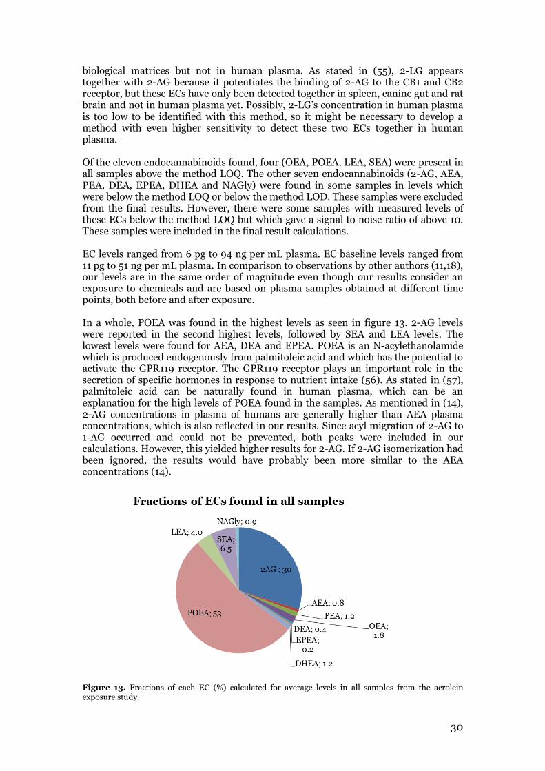
30

biological matrices but not in human plasma. As stated in (55), 2-LG appears together with 2-AG because it potentiates the binding of 2-AG to the CB1 and CB2 receptor, but these ECs have only been detected together in spleen, canine gut and rat brain and not in human plasma yet. Possibly, 2-LG’s concentration in human plasma is too low to be identified with this method, so it might be necessary to develop a method with even higher sensitivity to detect these two ECs together in human plasma. Of the eleven endocannabinoids found, four (OEA, POEA, LEA, SEA) were present in all samples above the method LOQ. The other seven endocannabinoids (2-AG, AEA, PEA, DEA, EPEA, DHEA and NAGly) were found in some samples in levels which were below the method LOQ or below the method LOD. These samples were excluded from the final results. However, there were some samples with measured levels of these ECs below the method LOQ but which gave a signal to noise ratio of above 10. These samples were included in the final result calculations. EC levels ranged from 6 pg to 94 ng per mL plasma. EC baseline levels ranged from 11 pg to 51 ng per mL plasma. In comparison to observations by other authors (11,18), our levels are in the same order of magnitude even though our results consider an exposure to chemicals and are based on plasma samples obtained at different time points, both before and after exposure. In a whole, POEA was found in the highest levels as seen in figure 13. 2-AG levels were reported in the second highest levels, followed by SEA and LEA levels. The lowest levels were found for AEA, DEA and EPEA. POEA is an N-acylethanolamide which is produced endogenously from palmitoleic acid and which has the potential to activate the GPR119 receptor. The GPR119 receptor plays an important role in the secretion of specific hormones in response to nutrient intake (56). As stated in (57), palmitoleic acid can be naturally found in human plasma, which can be an explanation for the high levels of POEA found in the samples. As mentioned in (14), 2-AG concentrations in plasma of humans are generally higher than AEA plasma concentrations, which is also reflected in our results. Since acyl migration of 2-AG to 1-AG occurred and could not be prevented, both peaks were included in our calculations. However, this yielded higher results for 2-AG. If 2-AG isomerization had been ignored, the results would have probably been more similar to the AEA concentrations (14).

Figure 13. Fractions of each EC (%) calculated for average levels in all samples from the acrolein exposure study.

31

The subjects were divided into two groups: the non-sensitive and sensitive subjects, and the average EC levels were calculated for each group, for each timepoint and for each exposure. The results are presented below (figure 14-16). Since no further statistical tests were carried out, it is not possible to draw conclusions regarding the significance of increasing or decreasing amounts in response to exposure. In general there were trends observed, which can also be seen when multivariate data analysis was performed as described in chapter 3.2.1, however further statistical tests are needed to confirm these presumptions. As seen in figure 14, baseline levels of each EC seem to be similar for non- sensitive and sensitive subjects, which is expected since no controlled exposure has taken place. After exposure there are some changes that can be observed, however this still needs to be confirmed with statistical tests. As seen in figure 15, SEA, LEA, NAGly and AEA levels seem to have remained almost the same directly after exposure compared to baseline levels for both groups and for both exposures. POEA levels were almost the same directly after exposure, except for the non-sensitive group. For the non-sensitive group, POEA levels after acrolein exposure increased slightly, while POEA levels after heptane exposure decreased to some extent compared to baseline levels. DHEA, EPEA, OEA, DEA and PEA levels increased to some degree for both groups and for both exposures after exposure. It seems as if these ECs are produced more numerously when exposed to a chemical, and it doesn’t seem to matter whether it is an irritant, as is acrolein, or a harmless chemical, as is heptane. 2-AG behaves somewhat differently. For sensitive subjects, 2-AG levels increased in relation to baseline levels both after acrolein and heptane exposure, while non-sensitive subjects’ levels remained rather the same compared to baseline levels. After heptane exposure this increase was bigger than after acrolein exposure. There seems to be an effect on 2-AG levels of sensitive subjects after any chemical exposure and not specifically after exposure of an irritant. 24 hours after exposure, plasma samples were also taken and measured (figure 16). SEA, LEA, AEA, PEA, OEA and DHEA levels were even lower than baseline levels 24 hours after exposure for both subject groups and exposure types. This suggests that an increase or a decrease in levels can also be related to stress. A possible explanation could be that before exposure the subjects might have been stressed out because they did not know what they were expecting so their levels were high while 24 hours after exposure they were relaxed so the levels went down to a possibly normal level again. EPEA levels after 24 hours decreased compared to EPEA baseline levels except for the sensitive subjects after heptane exposure who had a slightly higher EPEA level average after 24 hours. 2-AG average levels were lower after 24 hours than before exposure but for the non sensitive group after acrolein exposure the average level was even higher than before and after exposure. NAGly and DEA levels were the same as before exposure 24 hours after exposure. This suggests that NAGly and DEA levels are not influenced by stress. POEA levels increased 24 hours after exposure for both groups and both exposures. This suggests that stress decreases the levels instead of increasing the levels, while a relaxed state increases POEA levels again to a possibly normal level. Interestingly, there are no obvious differences observed between the non-sensitive and sensitive subjects, suggesting that the diagnosis does not affect EC levels. In some cases both acrolein and heptane have effects on the EC levels. This indicates that the levels do not necessarily increase/decrease because of an irritating chemical but most probably for other reasons such as stress or diet. The effect of stress on the levels could possibly be underlined by the BORG-CR-100 results which will be analyzed by the Department of Psychology at Umeå University.

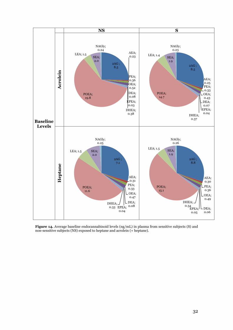
32

Baseline Levels

NS S

Ac

ro

lein

He

pta

ne

Figure 14. Average baseline endocannabinoid levels (ng/mL) in plasma from sensitive subjects (S) and non-sensitive subjects (NS) exposed to heptane and acrolein (+ heptane).

2AG ; 8.5

AEA; 0.23

PEA; 0.36

OEA; 0.52

DEA; 0.08

EPEA; 0.03

DHEA; 0.38

POEA; 19.8

LEA; 1.5 SEA; 2.0

NAGly; 0.24

2AG ; 8.5

AEA; 0.25 PEA; 0.33

OEA; 0.43

DEA; 0.07

EPEA; 0.04

DHEA; 0.37

POEA; 14.7

LEA; 1.4 SEA; 1.9

NAGly; 0.23

2AG ; 7.1

AEA; 0.31

PEA; 0.33

OEA; 0.47

DEA; 0.08 EPEA;

0.04

DHEA; 0.33

POEA; 11.6

LEA; 1.5 SEA; 2.0

NAGly; 0.25

2AG ; 8.8

AEA; 0.30

PEA; 0.36

OEA; 0.49

DEA; 0.06

EPEA; 0.05

DHEA; 0.34

POEA; 15.1

LEA; 1.5 SEA; 1.9

NAGly; 0.26

33

POSTLevels

NS S

Ac

ro

lein

He

pta

ne

Figure 15. Average post exposure endocannabinoid levels (ng/mL) in plasma from sensitive subjects (S) and non-sensitive subjects (NS) exposed to heptane and acrolein (+ heptane).

2AG ; 7.0

AEA; 0.26

PEA; 0.47

OEA; 0.60

DEA; 0.21

EPEA; 0.10

DHEA; 0.48

POEA; 14.5

LEA; 1.5 SEA; 2.5

NAGly; 0.30

2AG ; 12.3

AEA; 0.30

PEA; 0.48

OEA; 0.69 DEA;

0.23 EPEA;

0.11

DHEA; 0.48

POEA; 13.8

LEA; 1.4 SEA; 2.5

NAGly; 0.28

2AG ; 6.7

AEA; 0.26

PEA; 0.37

OEA; 0.58

DEA; 0.19

EPEA; 0.10

DHEA; 0.46

POEA; 8.2

LEA; 1.2 SEA; 2.2

NAGly; 0.26

2AG ; 17.8

AEA; 0.26 PEA;

0.42

OEA; 0.71 DEA;

0.20

EPEA; 0.09

DHEA; 0.48

POEA; 15.0

LEA; 1.3

SEA; 2.3 NAGly; 0.24

34

24Levels

NS S

Ac

ro

lein

He

pta

ne

Figure 16. Average 24 hour endocannabinoid levels (ng/mL) in plasma from sensitive subjects (S) and non-sensitive subjects (NS) exposed to heptane and acrolein (+ heptane).

2AG ; 10.8

AEA; 0.13

PEA; 0.23

OEA; 0.36

DEA; 0.09 EPEA;

0.06

DHEA; 0.24

POEA; 19.4

LEA; 0.44

SEA; 1.0 NAGly;

0.30

2AG ; 6.9

AEA; 0.14

PEA; 0.25

OEA; 0.42

DEA; 0.09

EPEA; 0.06 DHEA;

0.24

POEA; 15.3

LEA; 0.45

SEA; 1.1 NAGly;

0.22

2AG ; 5.9

AEA; 0.17

PEA; 0.25

OEA; 0.34

DEA; 0.06

EPEA; 0.07

DHEA; 0.25

POEA; 16.9

LEA; 0.64

SEA; 1.3

NAGly; 0.27

2AG ; 4.8

AEA; 0.12

PEA; 0.24

OEA; 0.41

DEA; 0.04

EPEA; 0.03

DHEA; 0.16

POEA; 17.5

LEA; 0.55

SEA; 1.4 NAGly;

0.21

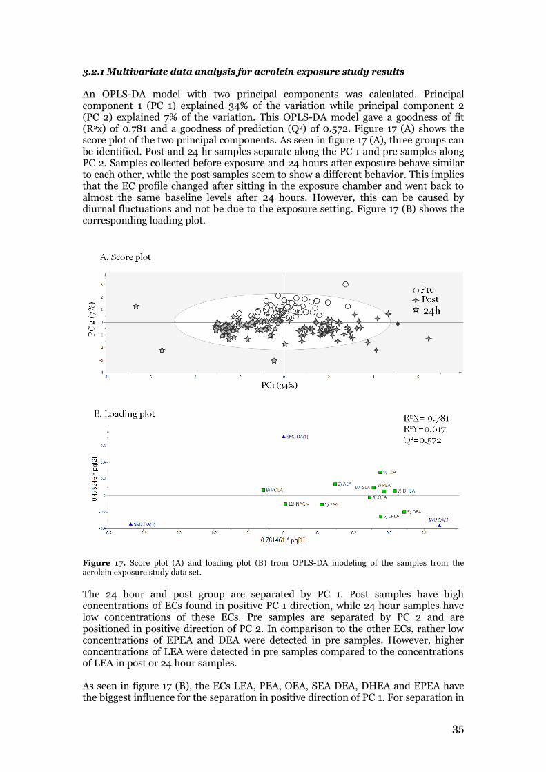
35

3.2.1 Multivariate data analysis for acrolein exposure study results

An OPLS-DA model with two principal components was calculated. Principal component 1 (PC 1) explained 34% of the variation while principal component 2 (PC 2) explained 7% of the variation. This OPLS-DA model gave a goodness of fit (R2x) of 0.781 and a goodness of prediction (Q2) of 0.572. Figure 17 (A) shows the score plot of the two principal components. As seen in figure 17 (A), three groups can be identified. Post and 24 hr samples separate along the PC 1 and pre samples along PC 2. Samples collected before exposure and 24 hours after exposure behave similar to each other, while the post samples seem to show a different behavior. This implies that the EC profile changed after sitting in the exposure chamber and went back to almost the same baseline levels after 24 hours. However, this can be caused by diurnal fluctuations and not be due to the exposure setting. Figure 17 (B) shows the corresponding loading plot.

Figure 17. Score plot (A) and loading plot (B) from OPLS-DA modeling of the samples from the acrolein exposure study data set.

The 24 hour and post group are separated by PC 1. Post samples have high concentrations of ECs found in positive PC 1 direction, while 24 hour samples have low concentrations of these ECs. Pre samples are separated by PC 2 and are positioned in positive direction of PC 2. In comparison to the other ECs, rather low concentrations of EPEA and DEA were detected in pre samples. However, higher concentrations of LEA were detected in pre samples compared to the concentrations of LEA in post or 24 hour samples. As seen in figure 17 (B), the ECs LEA, PEA, OEA, SEA DEA, DHEA and EPEA have the biggest influence for the separation in positive direction of PC 1. For separation in

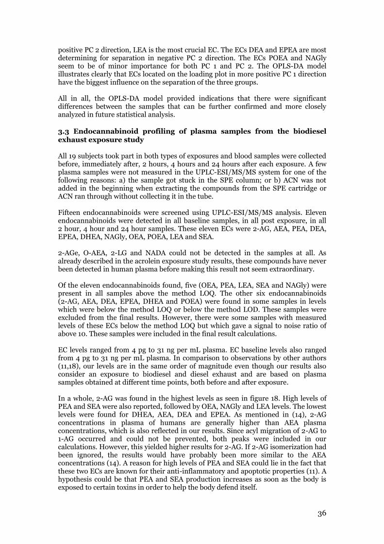
36

positive PC 2 direction, LEA is the most crucial EC. The ECs DEA and EPEA are most determining for separation in negative PC 2 direction. The ECs POEA and NAGly seem to be of minor importance for both PC 1 and PC 2. The OPLS-DA model illustrates clearly that ECs located on the loading plot in more positive PC 1 direction have the biggest influence on the separation of the three groups. All in all, the OPLS-DA model provided indications that there were significant differences between the samples that can be further confirmed and more closely analyzed in future statistical analysis.

3.3 Endocannabinoid profiling of plasma samples from the biodiesel exhaust exposure study All 19 subjects took part in both types of exposures and blood samples were collected before, immediately after, 2 hours, 4 hours and 24 hours after each exposure. A few plasma samples were not measured in the UPLC-ESI/MS/MS system for one of the following reasons: a) the sample got stuck in the SPE column; or b) ACN was not added in the beginning when extracting the compounds from the SPE cartridge or ACN ran through without collecting it in the tube. Fifteen endocannabinoids were screened using UPLC-ESI/MS/MS analysis. Eleven endocannabinoids were detected in all baseline samples, in all post exposure, in all 2 hour, 4 hour and 24 hour samples. These eleven ECs were 2-AG, AEA, PEA, DEA, EPEA, DHEA, NAGly, OEA, POEA, LEA and SEA. 2-AGe, O-AEA, 2-LG and NADA could not be detected in the samples at all. As already described in the acrolein exposure study results, these compounds have never been detected in human plasma before making this result not seem extraordinary. Of the eleven endocannabinoids found, five (OEA, PEA, LEA, SEA and NAGly) were present in all samples above the method LOQ. The other six endocannabinoids (2-AG, AEA, DEA, EPEA, DHEA and POEA) were found in some samples in levels which were below the method LOQ or below the method LOD. These samples were excluded from the final results. However, there were some samples with measured levels of these ECs below the method LOQ but which gave a signal to noise ratio of above 10. These samples were included in the final result calculations. EC levels ranged from 4 pg to 31 ng per mL plasma. EC baseline levels also ranged from 4 pg to 31 ng per mL plasma. In comparison to observations by other authors (11,18), our levels are in the same order of magnitude even though our results also consider an exposure to biodiesel and diesel exhaust and are based on plasma samples obtained at different time points, both before and after exposure. In a whole, 2-AG was found in the highest levels as seen in figure 18. High levels of PEA and SEA were also reported, followed by OEA, NAGly and LEA levels. The lowest levels were found for DHEA, AEA, DEA and EPEA. As mentioned in (14), 2-AG concentrations in plasma of humans are generally higher than AEA plasma concentrations, which is also reflected in our results. Since acyl migration of 2-AG to 1-AG occurred and could not be prevented, both peaks were included in our calculations. However, this yielded higher results for 2-AG. If 2-AG isomerization had been ignored, the results would have probably been more similar to the AEA concentrations (14). A reason for high levels of PEA and SEA could lie in the fact that these two ECs are known for their anti-inflammatory and apoptotic properties (11). A hypothesis could be that PEA and SEA production increases as soon as the body is exposed to certain toxins in order to help the body defend itself.

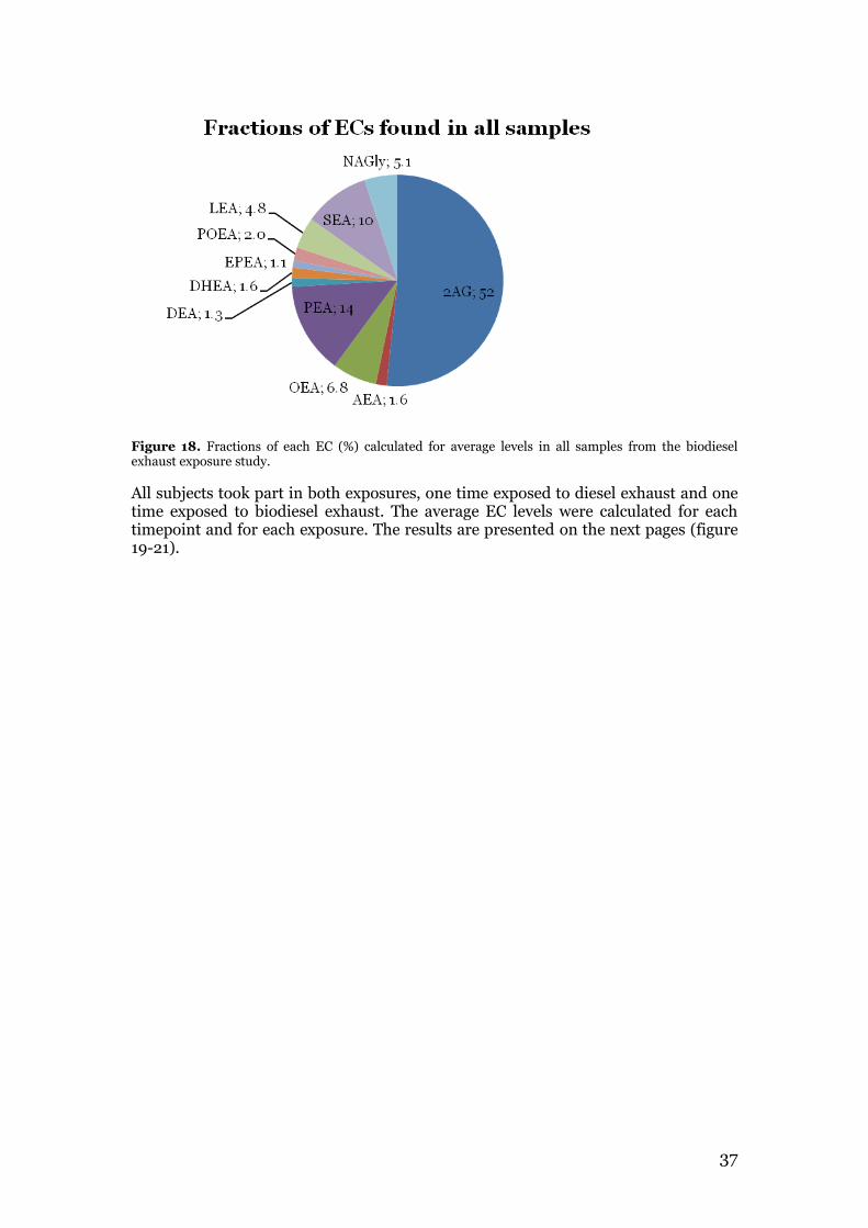
37

Figure 18. Fractions of each EC (%) calculated for average levels in all samples from the biodiesel exhaust exposure study.

All subjects took part in both exposures, one time exposed to diesel exhaust and one time exposed to biodiesel exhaust. The average EC levels were calculated for each timepoint and for each exposure. The results are presented on the next pages (figure 19-21).

38

2AG

Diesel Biodiesel

time ng/mL plasma ng/mL plasma

pre 7.39 6.45

post 7.59 6.17

2h 6.79 5.52

4h 7.71 7.51

24h 7.47 7.94

AEA

Diesel Biodiesel

time ng/mL plasma ng/mL plasma

pre 0.15 0.57

post 0.16 0.29

2h 0.14 0.29

4h 0.12 0.19

24h 0.14 0.22

OEA

Diesel Biodiesel

time ng/mL plasma ng/mL plasma

pre 0.91 0.76

post 1.12 1.02

2h 1.05 0.81

4h 1.32 0.67

24h 1.05 0.71

PEA

Diesel Biodiesel

time ng/mL plasma ng/mL plasma

pre 1.88 1.51

post 2.84 1.90

2h 2.34 1.53

4h 2.14 1.58

24h 1.94 1.57

Figure 19. Average endocannabinoid (2-AG, AEA, OEA, PEA) levels (ng/mL) in plasma from subjects exposed to diesel exhaust and biodiesel exhaust.

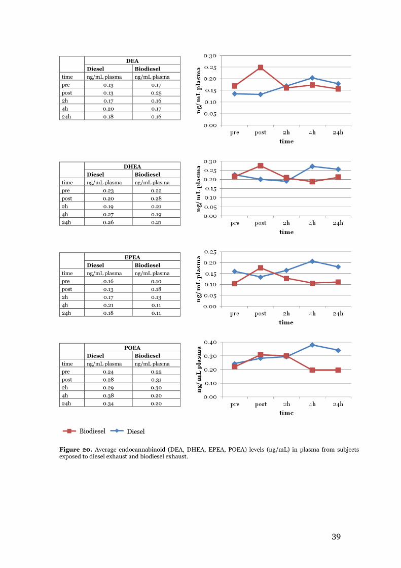
39

DEA

Diesel Biodiesel

time ng/mL plasma ng/mL plasma

pre 0.13 0.17

post 0.13 0.25

2h 0.17 0.16

4h 0.20 0.17

24h 0.18 0.16

DHEA

Diesel Biodiesel

time ng/mL plasma ng/mL plasma

pre 0.23 0.22

post 0.20 0.28

2h 0.19 0.21

4h 0.27 0.19

24h 0.26 0.21

EPEA

Diesel Biodiesel

time ng/mL plasma ng/mL plasma

pre 0.16 0.10

post 0.13 0.18

2h 0.17 0.13

4h 0.21 0.11

24h 0.18 0.11

POEA

Diesel Biodiesel

time ng/mL plasma ng/mL plasma

pre 0.24 0.22

post 0.28 0.31

2h 0.29 0.30

4h 0.38 0.20

24h 0.34 0.20

Figure 20. Average endocannabinoid (DEA, DHEA, EPEA, POEA) levels (ng/mL) in plasma from subjects exposed to diesel exhaust and biodiesel exhaust.

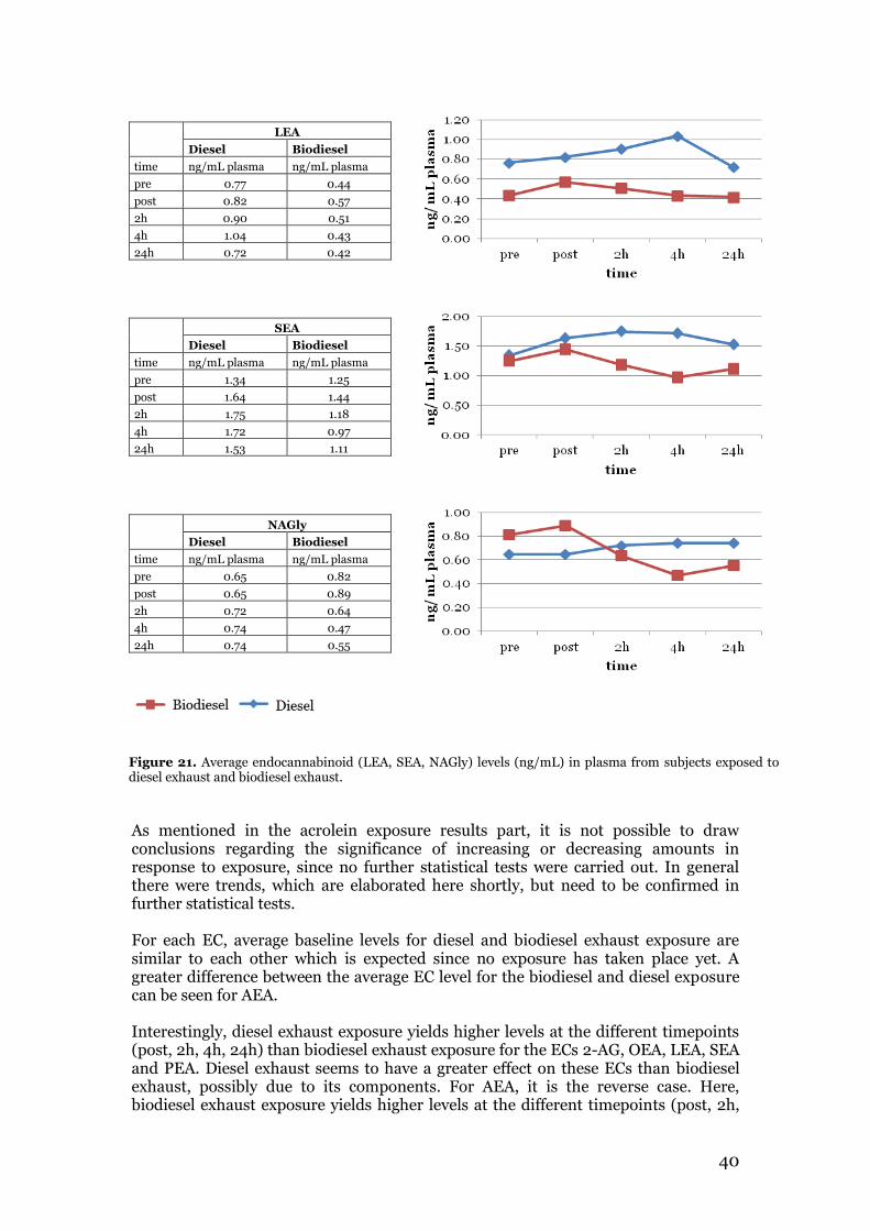
40

LEA

Diesel Biodiesel

time ng/mL plasma ng/mL plasma

pre 0.77 0.44

post 0.82 0.57

2h 0.90 0.51

4h 1.04 0.43

24h 0.72 0.42

SEA

Diesel Biodiesel

time ng/mL plasma ng/mL plasma

pre 1.34 1.25

post 1.64 1.44

2h 1.75 1.18

4h 1.72 0.97

24h 1.53 1.11

NAGly

Diesel Biodiesel

time ng/mL plasma ng/mL plasma

pre 0.65 0.82

post 0.65 0.89

2h 0.72 0.64

4h 0.74 0.47

24h 0.74 0.55

Figure 21. Average endocannabinoid (LEA, SEA, NAGly) levels (ng/mL) in plasma from subjects exposed to diesel exhaust and biodiesel exhaust.

As mentioned in the acrolein exposure results part, it is not possible to draw conclusions regarding the significance of increasing or decreasing amounts in response to exposure, since no further statistical tests were carried out. In general there were trends, which are elaborated here shortly, but need to be confirmed in further statistical tests. For each EC, average baseline levels for diesel and biodiesel exhaust exposure are similar to each other which is expected since no exposure has taken place yet. A greater difference between the average EC level for the biodiesel and diesel exposure can be seen for AEA. Interestingly, diesel exhaust exposure yields higher levels at the different timepoints (post, 2h, 4h, 24h) than biodiesel exhaust exposure for the ECs 2-AG, OEA, LEA, SEA and PEA. Diesel exhaust seems to have a greater effect on these ECs than biodiesel exhaust, possibly due to its components. For AEA, it is the reverse case. Here, biodiesel exhaust exposure yields higher levels at the different timepoints (post, 2h,

41

4h, 24h) than diesel exhaust exposure, however there seems to be a decrease in levels instead of an increase. For the other ECs (DEA, DHEA, EPEA, POEA and NAGly) there is no general trend for biodiesel exhaust or diesel exhaust. An interesting observation to mention as well, is that for diesel exhaust exposure most EC levels seem to fall considerably after 24 hours compared to the 4h timepoint, while for biodiesel exhaust exposure these levels increase after 24 hours again compared to the other timepoints. There seems to be a difference between diesel and biodiesel and their effect on ECs, which can be clarified in further research and further statistical tests. For some ECs (including OEA, DEA, DHEA, EPEA, POEA, LEA, NAGly) and after diesel exposure, the highest level is reached after 4 hours. For others (including SEA and AEA) the highest level is reached 2 hours after diesel exhaust exposure. For 2-AG and PEA the highest levels are obtained directly after the exposure. This suggests that the response to diesel exhaust might take a different length of time depending on the EC. It seems interesting that for biodiesel exhaust exposure, the levels of almost all ECs (except 2-AG and AEA levels) increase directly after exposure, then fall down after 2 and/or 4 hours after exposure but then go up again after 24 hour exposure. Therefore the highest levels after biodiesel exhaust exposure are either obtained directly after or 24 hours after exposure. It also suggests that biodiesel exhaust exposure has a direct response on the EC levels compared to diesel exhaust which has a longer response time for some ECs.

3.4 Summary and comparison of acrolein exposure and biodiesel exhaust exposure results with relation to aim of study Firstly, this was the first validated method with the ability to analyze 15 endocannabinoids in a single injection. In all human plasma samples, obtained from both studies, it was possible to detect and quantify 11 of the 15 endocannabinoids including AEA, 2-AG, OEA, PEA, SEA, DHEA, EPEA, POEA, LEA, DEA and NAGly. In Balvers et al. (10), an LC-MS/MS method was developed and validated to determine 12 endocannabinoids in plasma. In comparison to both the acrolein exposure and biodiesel exhaust exposure results, Balvers et al. (10) did not report human plasma samples with quantifiable concentrations of DEA and NAGly. An explanation for this could be the use of different equipment and use of different samples. However, Balvers et al. (10), also did not observe 2-AGe, O-AEA and NADA, which corresponds to our results from both studies. Of the endocannabinoids we focused on, only AEA, 2-AG, OEA, PEA, SEA, DHEA, have been possible to detect in quantifiable levels in human plasma so far (10,58). LEA has been implemented in a LC-MS/MS for the analysis of endocannabinoids in human plasma but has not been measured in real human plasma samples (16). It has never been possible to quantify EPEA, DEA, NAGly and POEA in human plasma before which was possible with our method, however, only in very low concentrations. For these compounds, many of the samples had to be excluded in the final calculations because their signal to noise was too low or the levels were lower than the LOD. Therefore, it could be a goal to develop an even more sensitive method in order to detect these ECs even at such low levels.

42

Interestingly, POEA was detected in the highest levels in the acrolein study while in the biodiesel exhaust exposure study it was detected with levels in the lower part of the middle range. POEA levels must be higher when exposed to chemicals such as acrolein or heptane instead of biodiesel or diesel exhaust. In both studies, however, the average EPEA levels were found to be the lowest of all ECs. Furthermore, measured NAGly and PEA levels seem to be overall higher in the biodiesel exhaust exposure study compared to the acrolein exposure study since all NAGly and PEA levels were above the method LOQ in the biodiesel exhaust exposure study. As seen both in the absolute concentrations in the acrolein study and in the results obtained from multivariate data analysis, there seems to be a difference in most EC levels after exposure to any chemical, and it does not matter whether it is an irritant such as acrolein or only heptane. However, the levels of some ECs do not seem to be influenced by acrolein or heptane exposure at all. Interesting is also that between sensitive and non-sensitive subjects there does not seem to be a difference, except possibly in the 2-AG levels. Some ECs have lower 24 hour levels than baseline levels, while others have the reversed case. An explanation could be that the EC levels are also related to stress and decrease or increase as soon as the subject is in a relaxed state. The biodiesel exhaust exposure results show that there seems to be a difference between the EC levels after biodiesel and diesel exhaust exposure. For some ECs, diesel exhaust seems to have a greater effect on the levels than biodiesel exhaust has. Some EC levels seem to increase or decrease faster after biodiesel exhaust exposure than after diesel exhaust exposure, suggesting that it takes more time for the body’s ECs to respond to diesel than to biodiesel. All these observations should be further examined in future research including more statistical tests since there seem to be differences in EC levels observed after exposure to either acrolein, heptane, diesel or biodiesel. Table 4 shows an overview of the EC concentration ranges observed in the human plasma samples from both studies. It seems that overall higher EC levels were measured in the biodiesel exhaust exposure than in the acrolein exposure study, since the upper level seems to be higher for almost all ECs. However, for POEA, 2-AG and DHEA, the upper values were higher in the acrolein exposure study. The difference in values can either be explained by the different chemicals (acrolein/heptane vs. biodiesel/diesel) or by the different types of subjects (healthy vs. chemical sensitive/healthy subjects) but this has to be examined further. In both the acrolein exposure and the biodiesel exhaust exposure study, the EC levels were in the same order of magnitude that has been reported for EC levels in the literature (11,18,58).

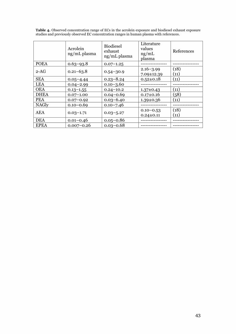
43

Table 4. Observed concentration range of ECs in the acrolein exposure and biodiesel exhaust exposure studies and previously observed EC concentration ranges in human plasma with references.

Acrolein ng/mL plasma

Biodiesel exhaust ng/mL plasma

Literature values ng/mL plasma

References

POEA 0.63–93.8 0.07–1.25 ---------------- ----------------

2-AG 0.21–63.8 0.54–30.9 2.16–3.99 7.09±12.39

(18) (11)

SEA 0.05–4.44 0.23–8.24 0.52±0.18 (11) LEA 0.04–2.99 0.10–3.60 ---------------- ---------------- OEA 0.13–1.55 0.24–10.2 1.37±0.43 (11) DHEA 0.07–1.00 0.04–0.69 0.17±0.16 (58) PEA 0.07–0.92 0.03–6.40 1.39±0.36 (11) NAGly 0.10–0.69 0.10–7.46 ---------------- ----------------

AEA 0.03–1.71 0.03–5.27 0.10–0.53 0.24±0.11

(18) (11)

DEA 0.01–0.46 0.05–0.86 ---------------- ---------------- EPEA 0.007–0.26 0.03–0.68 ---------------- ----------------

44

4. Conclusions

We developed an UPLC-ESI/MS/MS method to detect 13 oxylipins simultaneously in biological samples. Our primary goal was to develop a method for the analysis of 16 oxylipins which we did not manage to do since it was not possible to separate all 16 oxylipins with the developed method. The developed and validated method showed good sensitivity and linearity, was accurate and precise and had recoveries in a reasonable range (with exception of one compound). A previously developed and validated method for the analysis of 15 endocannabinoids was applied for the quantification of endocannabinoids in human plasma samples obtained from two studies, the acrolein exposure and the biodiesel exhaust exposure study. Of the 15 endocannabinoids, 11 endocannabinoids were possible to detect and quantify in the human plasma samples from both studies. In the acrolein exposure study, EC levels between 6 and 94 ng/mL plasma were observed. POEA was detected in the highest average levels, while EPEA was detected in the lowest average level. Since no statistical tests were carried out, only presumptions relating to differences in levels could be made. There seems to be no obvious difference between sensitive and non-sensitive subjects when exposed to either acrolein or heptane. Heptane seems to have a similar effect as acrolein on all subjects’ EC levels. There are EC levels which increase or decrease directly after exposure to either heptane or acrolein but there are also EC levels which remain constant. Most EC levels in plasma samples taken after 24 hours, were lower than baseline levels, suggesting that EC levels could also be related to other factors such as stress. The described OPLS-DA model was a first approach to draw more clear conclusions on the results obtained from the acrolein study. The model shows three groups: pre, post and 24 hours. The 24 hour and the pre samples behave similar to each other, while the post samples stand out more, suggesting that the subject’s EC profile changed after sitting in the exposure chamber. The ECs LEA, PEA, OEA, SEA, DEA, DHEA and EPEA have the biggest influence on the separation of the three groups. In the biodiesel exhaust exposure study, EC levels between 4 and 31 ng/mL plasma were observed. 2-AG was detected in the highest average level, while EPEA was detected in the lowest average level. Both diesel exhaust and biodiesel exhaust seem to have had an effect on the EC levels of the subjects. For most ECs, diesel exhaust yielded higher levels after exposure than biodiesel exhaust exposure, with an increase of levels at the different time points. AEA seems to react differently. For AEA, higher values after biodiesel exhaust exposure were measured but a decrease in the temporal trend was observed. For most ECs after diesel exhaust exposure, the levels decrease after 24 hours compared to 4 hours while after biodiesel exhaust exposure there is an increase. For most ECs after biodiesel exhaust exposure, the highest level is reached directly after exposure while after diesel exhaust exposure, the highest level is either reached directly after exposure, 2 hours after exposure or 4 hours after exposure, suggesting a different reaction time of the ECs to biodiesel and diesel exhaust.

45

5. Future perspectives

The developed and validated method for the analysis of oxylipins can be applied to analyze oxylipins in the same human plasma samples that have been analyzed for endocannabinoids during the course of the diploma work. By doing this, it will be possible to obtain an even more comprehensive metabolic profile that will enable more information on bioactive lipids and their role in the human body. Furthermore, the developed methods can be applied to analyze endocannabinoids and oxylipins in other biological matrices of interest such as tissues, cells or saliva. In order to make the developed and validated method for the analysis of oxylipins even more sensitive, it will be necessary to change the equipment and repeat validation of the method. Since there is a new and more effective UPLC-MS/MS equipment being introduced at the University, this will be a future task. With the results obtained from both studies, it is necessary to carry out more statistical analysis to establish if the levels increased or decreased and to confirm the presumptions made. Since the analysis of endocannabinoids was a sub-study of the acrolein exposure study, it will be necessary to include the results from the other tests (such as determing the stress level with the Borgs scale) to determine a relationship to the metabolic profile. After including the other results, it may be possible to divide the subjects into other groups which can lead to different and refined results in multivariate data analysis. Furthermore, it would be interesting to see if the effect of acrolein and heptane is in fact similar on the EC levels, if the EC levels are possibly more related to stress than to a chemical and if there is really not a difference between sensitive and non sensitive subjects. These assumptions can all be clarified in further research and statistical tests. Analyzing endocannabinoids in human plasma samples from the biodiesel exhaust exposure study was also one of many assay methods to determine the health effects of biodiesel compared to diesel exhaust. It is therefore necessary to determine all observed endpoints before drawing definite conclusions on the health effects. Since both diesel and biodiesel exhaust exposure seem to have had an effect on the EC levels, it would be interesting to carry out more statistical tests (including multivariate data analysis) to prove the assumptions.

46

Acknowledgements

First and foremost, I would like to thank my supervisors at Umeå University, Malin L. Nording and Sandra Gouveia. Malin, thank you for giving me the opportunity to complete my thesis in your working group and thank you for your wonderful support, feedback and guidance. Sandra, thank you for being a great supervisor in the lab, for your valuable help and advice and for all the fun times. Secondly, I would like to thank my supervising professor in Stuttgart, Prof. Dr. Walter Vetter for helping to organize the diploma project in Sweden and for his kind advice. I would also like to thank our collaborators Anna-Sara Claeson and co-workers at the Department of Psychology at Umeå University, Jenny Bosson and co-workers at the Department of Public Health and Clinical Medicine at Norrlands University Hospital and Christoffer Boman and Robin Nystrom at the Department of Applied Physics and Electronics at Umeå University. The Swedish Research Council Formas and ERASMUS Placement are also gratefully acknowledged for their financial support. A special thanks goes out to my parents and my sister for always being there for me, for always believing in me and encouraging me on my way to reach my goal. I am also grateful for all the friends I made during the course of my studies; thank you for the fun and memorable times. Last but not least, I would like to thank Hans. You were always here for me no matter what. Thank you for your unconditional support.

47

References

1) Evans, J. F., & Hutchinson, J. H. (2010). Seeing the future of bioactive lipid drug targets. Nature Chemical Biology, 6(7), 476–9 2) Murakami, M. (2011). Lipid mediators in life science. Experimental animals / Japanese Association for Laboratory Animal Science, 60(1), 7–20 3) Zivkovic, A. M., Telis, N., German, J. B., & Hammock, B. D. (2011). Dietary omega-3 fatty acids aid in the modulation of inflammation and metabolic health. California Agriculture, 65(3), 106–111. 4) Yang, J., Schmelzer, K., Georgi, K., & Hammock, B. D. (2009). Quantitative Profiling Method for Oxylipin Metabolome by Liquid Chromatography Electrospray Ionization Tandem Mass Spectrometry, 81(19), 8085–8093. 5) Yang, J., Dong, H., & Hammock, B. D. (2011). Profiling the regulatory lipids: another systemic way to unveil the biological mystery. Current opinion in lipidology, 22(3), 197–203. 6) Shinde, D. D., Kim, K., Oh, K., Abdalla, N., Liu, K., Kyung, S., Shon, J., et al. (2012). LC – MS / MS for the simultaneous analysis of arachidonic acid and 32 related metabolites in human plasma : Basal plasma concentrations and aspirin-induced changes of eicosanoids. Journal of Chromatography B, 911, 113–121. 7) Strassburg, K., Huijbrechts, A. M. L., Kortekaas, K. a, Lindeman, J. H., Pedersen, T. L., Dane, A., Berger, R., et al. (2012). Quantitative profiling of oxylipins through comprehensive LC-MS/MS analysis: application in cardiac surgery. Analytical and bioanalytical chemistry, 404(5), 1413–26. 8) Zivkovic, A. M., Yang, J., Georgi, K., Hegedus, C., Nording, M. L., O’Sullivan, A., German, J. B., et al. (2012). Serum oxylipin profiles in IgA nephropathy patients reflect kidney functional alterations. Metabolomics, 8(6), 1102–1113. 9) Fanelli, F., Lallo, V. D. Di, Belluomo, I., Iasio, R. De, Casadio, E., Gasparini, D. I., Colavita, M., et al. (2012). Estimation of reference intervals of fi ve endocannabinoids and endocannabinoid related compounds in human plasma by two dimensional-LC / MS / MS, 53, 481–493 10) Kingsley, P. J., & Marnett, L. J. (2009). Analysis of endocannabinoids, their congeners and COX-2 metabolites. Journal of chromatography. B, Analytical technologies in the biomedical and life sciences, 877(26), 2746–54. 11) Balvers, M. G. J., Verhoeckx, K. C. M., & Witkamp, R. F. (2009). Development and validation of a quantitative method for the determination of 12 endocannabinoids and related compounds in human plasma using liquid chromatography-tandem mass spectrometry. Journal of chromatography. B, Analytical technologies in the biomedical and life sciences, 877(14-15), 1583–90. 12) Williams, J., Wood, J., Pandarinathan, L., Karanian, D. a, Bahr, B. a, Vouros, P., & Makriyannis, A. (2007). Quantitative method for the profiling of the endocannabinoid metabolome by LC-atmospheric pressure chemical ionization-MS. Analytical chemistry, 79(15), 5582–93.

48

13) Amoako, A. a, Marczylo, T. H., Lam, P. M. W., Willets, J. M., Derry, A., Elson, J., & Konje, J. C. (2010). Quantitative analysis of anandamide and related acylethanolamides in human seminal plasma by ultra-performance liquid chromatography tandem mass spectrometry. Journal of chromatography. B, Analytical technologies in the biomedical and life sciences, 878(31), 3231–7. 14) Zoerner, A. a, Gutzki, F.-M., Batkai, S., May, M., Rakers, C., Engeli, S., Jordan, J., et al. (2011). Quantification of endocannabinoids in biological systems by chromatography and mass spectrometry: a comprehensive review from an analytical and biological perspective. Biochimica et biophysica acta, 1811(11), 706–23. 15) Brown, I., Cascio, M. G., Wahle, K. W. J., Smoum, R., Mechoulam, R., Ross, R. a, Pertwee, R. G., et al. (2010). Cannabinoid receptor-dependent and -independent anti-proliferative effects of omega-3 ethanolamides in androgen receptor-positive and -negative prostate cancer cell lines. Carcinogenesis, 31(9), 1584–91. 16) Palandra, J., Prusakiewicz, J., Ozer, J. S., Zhang, Y., & Heath, T. G. (2009). Endogenous ethanolamide analysis in human plasma using HPLC tandem MS with electrospray ionization. Journal of chromatography. B, Analytical technologies in the biomedical and life sciences, 877(22), 2052–60. 17) Tortoriello, G., Rhodes, B. P., Takacs, S. M., Stuart, J. M., Basnet, A., Raboune, S., Widlanski, T. S., et al. (2013). Targeted Lipidomics in Drosophila melanogaster Identifies Novel 2-Monoacylglycerols and N-acyl Amides. PloS one, 8(7) 18) Giroud, C., & Staub, C. (2009). Quantitative and qualitative profiling of endocannabinoids in human plasma using a triple quadrupole linear ion trap mass spectrometer with liquid chromatography, 629–638. 19) Jian, W., Edom, R., Weng, N., Zannikos, P., Zhang, Z., & Wang, H. (2010). Validation and application of an LC-MS/MS method for quantitation of three fatty acid ethanolamides as biomarkers for fatty acid hydrolase inhibition in human plasma. Journal of chromatography. B, Analytical technologies in the biomedical and life sciences, 878(20), 1687–99. 20) Nomura, D. K., Morrison, B. E., Blankman, J. L., Long, J. Z., Kinsey, S. G., Marcondes, M. C. G., Ward, A. M., et al. (2011). Endocannabinoid hydrolysis generates brain prostaglandins that promote neuroinflammation. Science (New York, N.Y.), 334(6057), 809–13. 21) Garrett-Meyer, E., Hidalgo, M., Eckhardt, S.G., Clendennin, N. (2011) Principles of Anticancer Drug Development. Springer 22) http://www.waters.com/waters/partDetail.htm?partNumber=186003365; accessed July 5th, 2013 23) http://www.isco.com/WebProductFiles/Applications/105/ Application_Notes/HPLC_System_Configuration.pdf; accessed June 13th, 2013 24) Vixom, L. Robert, Gehrke, W. C. (n.d.). Chromatography: A Science of Discovery 25) Harvey, David. (2000). Modern Analytical Chemistry. McGraw-Hill Companies

49

26) Eidhammer, Ingvar; Barsnes, Harald; Eide, E. G., & Martens, L. (n.d.). Computational and Statistical Methods for Protein Quantification by Mass Spectrometry. 27) http://www.jic.ac.uk/services/metabolomics/topics/lcms/why.htm; accessed June 13th, 2013 28) Ho, C. S., Lam, C. W. K., Chan, M. H. M., Cheung, R. C. K., Law, L. K., Lit, L. C. W., Ng, K. F., et al. (2003). Electrospray ionisation mass spectrometry: principles and clinical applications. The Clinical biochemist. Reviews / Australian Association of Clinical Biochemists, 24(1), 3–12 29) http://ccc.chem.pitt.edu/wipf/Agilent%20LC-MS%20primer.pdf; accessed June 13th, 2013 30) http://www.astbury.leeds.ac.uk/facil/MStut/mstutorial.htm; accessed June 13th, 2013 31) Schreiber, A. (n.d.). Advantages of Using Triple Quadrupole over Single Quadrupole Mass Spectrometry to Quantify and Identify the Presence of Pesticides in Water and Soil Samples. 32) Methods, A. (n.d.). Lod/loq, 2. 33) Green, J. M. (1996). Analytical Method Validation, (2). 34) Lehtonen, M., Storvik, M., Malinen, H., Hyytiä, P., Lakso, M., Auriola, S., Wong, G., et al. (2011). Determination of endocannabinoids in nematodes and human brain tissue by liquid chromatography electrospray ionization tandem mass spectrometry. Journal of chromatography. B, Analytical technologies in the biomedical and life sciences, 879(11-12), 677–94. 35) http://www.umetrics.com/default.aspx?id=8519&refid=7940; accessed June 13th, 2013 36) http://www.chemsec.org/hazardous-chemicals/health-implications; accessed June 11th, 2013 37) http://www.noharm.org/us_canada/issues/chemicals/#fn1; accessed June 11th, 2013 38) http://www.webmd.com/allergies/multiple-chemical-sensitivity; accessed June 11th, 2013 39) Valkenburg, E. (2010). Understanding Multiple Chemical Sensitivity: Causes, Effects, Personal Experiences and Resources. 40) Matthews, L. B. (n.d.). Chemical Sensitivity: A Guide to Coping With Hypersensitivity Syndrome, Sick Building Syndrome and Other Environmental Illnesses. 41) http://www.state.nj.us/dep/dsr/njcrp/acrolein.pdf; accessed June 11th, 2013 42) Harte, J. (n.d.). Toxics A to Z: A Guide to Everyday Pollution Hazards.

50

43) http://www.who.int/mediacentre/factsheets/fs313/en/; accessed June 11th, 2013 44) Traviss, N., Thelen, B. A., Ingalls, J. K., & Treadwell, M. D. (2010). Biodiesel versus Diesel: A Pilot Study Comparing Exhaust Exposures for Employees at a Rural Municipal Facility. Journal of the Air & Waste Management Association, 60(9), 1026–1033. 45) http://www.cdc.gov/niosh/docs/88-116/; accessed June 12th, 2013 46) http://www.sciencedaily.com/releases/2008/06/080604114550.htm; accessed June 12th, 2013 47) Ma, F., & Hanna, M. A. (1999). Biodiesel production : a review 1, 70, 1–15. 48) Swanson, K. J., Madden, M. C., & Ghio, A. J. (2007). Biodiesel exhaust: the need for health effects research. Environmental health perspectives, 115(4), 496–9. 49) Sharp, C. (1998) Characterization of Biodiesel Exhaust Emissions for EPA 211(b). Report. San Antonio, Tx: Southwest Research Institute 50) Di, Y., Cheung, C. S., & Huang, Z. (2009). Experimental investigation on regulated and unregulated emissions of a diesel engine fueled with ultra-low sulfur diesel fuel blended with biodiesel from waste cooking oil. The Science of the total environment, 407(2), 835–46. 51) Div. of Respiratory Medicine and Allergy, Norrlands University Hospital. (2012). Study Protocol: Cardiovascular and Pulmonary Effects of 100% Biodiesel Exhaust 52) Tiyapongpattana, W., Wilairat, P. and Marriott, P. J. (2008), Characterization of biodiesel and biodiesel blends using comprehensive two-dimensional gas chromatography. J. Sep. Science, 31: 2640–2649. 53) Brose, S. a, Thuen, B. T., & Golovko, M. Y. (2011). LC/MS/MS method for analysis of E₂ series prostaglandins and isoprostanes. Journal of lipid research, 52(4), 850–9. 54) Richardson, D., Ortori, C. a, Chapman, V., Kendall, D. a, & Barrett, D. a. (2007). Quantitative profiling of endocannabinoids and related compounds in rat brain using liquid chromatography-tandem electrospray ionization mass spectrometry. Analytical biochemistry, 360(2), 216–26. 55) Ben-Shabat, S., Fride, E., Sheskin, T., Tamiri, T., Rhee, M. H., Vogel, Z., Bisogno, T., et al. (1998). An entourage effect: inactive endogenous fatty acid glycerol esters enhance 2-arachidonoyl-glycerol cannabinoid activity. European journal of pharmacology, 353(1), 23–31. 56) Syed, S. K., Bui, H. H., Beavers, L. S., Farb, T. B., Ficorilli, J., Chesterfield, A. K., Kuo, M.-S., et al. (2012). Regulation of GPR119 receptor activity with endocannabinoid-like lipids. American journal of physiology. Endocrinology and metabolism, 303(12), E1469–78.

51

57) Nestel, P., Clifton, P., & Noakes, M. (1994). Effects of increasing dietary palmitoleic acid compared with palmitic and oleic acids on plasma lipids of hypercholesterolemic men. Journal of lipid research, 35(4), 656–62. 58) Balvers, M. G. J., Verhoeckx, K. C. M., Plastina, P., Wortelboer, H. M., Meijerink, J., & Witkamp, R. F. (2010). Docosahexaenoic acid and eicosapentaenoic acid are converted by 3T3-L1 adipocytes to N-acyl ethanolamines with anti-inflammatory properties. Biochimica et biophysica acta, 1801(10), 1107–14.

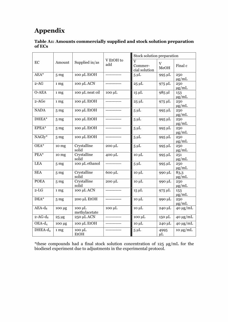
Appendix

Table A1: Amounts commercially supplied and stock solution preparation of ECs

EC Amount Supplied in/as V EtOH to add

Stock solution preparation

V Commer-cial solution

V MeOH

Final c

AEA* 5 mg 100 µL EtOH ----------- 5 µL 995 µL 250 µg/mL

2-AG 1 mg 100 µL ACN ----------- 25 µL 975 µL 250 µg/mL

O-AEA 1 mg 100 µL neat oil 100 µL 15 µL 985 µl 153 µg/mL

2-AGe 1 mg 100 µL EtOH ----------- 25 µL 975 µL 250 µg/mL

NADA 5 mg 100 µL EtOH ----------- 5 µL 995 µL 250 µg/mL

DHEA* 5 mg 100 µL EtOH ----------- 5 µL 995 µL 250 µg/mL

EPEA* 5 mg 100 µL EtOH ----------- 5 µL 995 µL 250 µg/mL

NAGly* 5 mg 100 µL EtOH ----------- 5 µL 995 µL 250 µg/mL

OEA* 10 mg Crystalline solid

200 µL 5 µL 995 µL 250 µg/mL

PEA* 10 mg Crystalline solid

400 µL 10 µL 995 µL 251 µg/mL

LEA 5 mg 100 µL ethanol ----------- 5 µL 995 µL 250 µg/mL

SEA 5 mg Crystalline solid

600 µL 10 µL 990 µL 83,3 µg/mL

POEA 5 mg Crystalline solid

200 µL 10 µL 990 µL 250 µg/mL

2-LG 1 mg 100 µL ACN ----------- 15 µL 975 µL 153 µg/mL

DEA* 5 mg 200 µL EtOH ----------- 10 µL 990 µL 250 µg/mL

AEA-d8 100 µg 100 µL methylacetate

100 µL

10 µL 240 µL 40 µg/mL

2-AG-d8 25 µg 250 µL ACN ----------- 100 µL 150 µL 40 µg/mL

OEA-d4 100 µg 100 µL EtOH ----------- 10 µL 240 µL 40 µg/mL

DHEA-d4 1 mg 100 µL EtOH

----------- 5 µL 4995 µL

10 µg/mL

*these compounds had a final stock solution concentration of 125 µg/mL for the biodiesel experiment due to adjustments in the experimental protocol.

Table A2: Amounts commercially supplied and stock solution preparation of oxylipins

Oxylipin Amount Supplied in/as V EtOH to add

Final c stock solution [µg/mL]

TXB2-d4 25 µg 250 µL Methylacetate 250 µL 100

TXB2 1 mg Crystalline solid 0.789 g 1000

PGE2 d4 50 µg 100 µL Methylacetate 100 µL 500

8-iso-PGE2 500 µg Crystalline solid 0.789 g 1000

8-iso-PGF2α 1 mg Crystalline solid 0.3945 g 1000

PGE2 1 mg Crystalline solid 0.789 g 1000

PGD2 1 mg Crystalline solid 0.789 g 1000

12,13-DiHOME-d4 25 µg 250 µL Methylacetate 250 µL 100

12,13-DiHOME 25 µg 250 µL Methylacetate 250 µL 100

9(S)-HODE-d4 25 µg 250 µL EtOH ----------- 100

12(S)-HEPE 25 µg 250 µL EtOH ----------- 1000

13-HODE 100 µg 100 µL EtOH ----------- 100

9(S)-HODE 100 µg 100 µL EtOH ----------- 1000

15-HETE 25 µg 250 µL EtOH ----------- 100

17-HDoHE 25 µg 250 µL EtOH ----------- 100

9-oxo-ODE 25 µg 250 µL EtOH ----------- 100

12-oxo-ETE 25 µg 250 µL EtOH ----------- 100

12-HETE 25 µg 250 µL EtOH ----------- 100

5-HETE 25 µg 250 µL EtOH ----------- 100

12(13)-EpOME-d4 25 µg Methylacetate 250 µL 100

12(13)-EpOME 25 µg Methylacetate 250 µL 100

CUDA 5000 µg Crystalline solid 15 mL 333

Table A3: Stock solution concentrations and preparation of standard solution 1 for oxylipins

Oxylipin Stock solution concentration (µg/mL)

V ( µL) C (µg/mL)

TXB2 1000 50 43

8-iso-PGF2a 1000 50 43

8-iso-PGE2 1000 50 43

PGE2 1000 50 43

PGD2 1000 50 43

12(S)-HEPE 100 100 8.7

13-HODE 1000 50 43

9(S)-HODE 1000 50 43

15-HETE 100 100 8.7

17-HDOHE 100 100 8.7

9-oxoODE 100 100 8.7

12-HETE 100 100 8.7

5-HETE 100 100 8.7

12-OxoETE 100 100 8.7

12,13-EPOME 100 100 8.7

Table A4: Calibration solution preparation for standards with stock solution concentration of 100 µg/mL

Standard c (µg/mL)

V Sn-1 (µL)

V MeOH (µL)

V final (µL)

C in vial (µg/µL)

M on column (µg)

Ng on column

Pg on column

S1 8.7

1150 0.0071 0.071 71 71000

S2 1.7 200 800 1000 0.0014 0.014 14 14000

S3 0.87 500 500 1000 0.00071 0.0071 7.1 7100

S4 0.44 500 500 1000 0.00036 0.0036 3.6 3600

S5 0.22 500 500 1000 0.00018 0.0018 1.8 1800

S6 0.11 500 500 1000 0.000089 0.00089 0.89 890

S7 0.054 500 500 1000 0.000044 0.00044 0.44 440

S8 0.027 500 500 1000 0.000022 0.00022 0.22 220

S9 0.014 500 500 1000 0.000011 0.00011 0.11 110

S10 0.0068 500 500 1000 0.0000056 0.000056 0.056 56

S11 0.0034 150 0.0000028 0.000028 0.028 28

Table A5: Calibration solution preparation for standards with stock solution concentration of 1000 µg/mL

Standard c (µg/mL)

V Sn-1 (µL)

V MeOH (µL)

V final (µL)

C in vial (µg/µL)

M on column (µg)

Ng on column

Pg on column

S1 43 1150 0.036 0.36 360 360000

S2 8.7 200 800 1000 0.0071 0.071 71 71100

S3 4.3 500 500 1000 0.0036 0.036 36 36000

S4 2.2 500 500 1000 0.0018 0.018 18 18000

S5 1.1 500 500 1000 0.00089 0.0089 8.9 8900

S6 0.54 500 500 1000 0.00044 0.0044 4.4 4400

S7 0.27 500 500 1000 0.00022 0.0022 2.2 2200

S8 0.14 500 500 1000 0.00011 0.0011 1.1 1100

S9 0.068 500 500 1000 0.000056 0.0006 0.56 560

S10 0.034 500 500 1000 0.000028 0.0003 0.28 280

S11 0.017 150 0.000014 0.0001 0.14 140

Table A6: Preparation of standard solutions (concentrations apply for 250 µg/mL stock solutions)

Calibration solutions

Standard c (µg/mL)

V Sn-1 (mL)

V final (mL)

V MeOH (mL)

S1 17 0.1 1.5 0

S1a 8.3 0.5 1 0.5

S2 3.3 0.2 1 0.8

S3 0.67 0.2 1 0.8

S4 0.13 0.2 1 0.8

S5 0.067 0.25 0.5 0.25

S6 0.033 0.25 0.5 0.25

S7 0.017 0.25 0.5 0.25

S8 0.0083 0.25 0.5 0.25

S9 0.0042 0.25 0.5 0.25

S10 0.0021 0.25 0.5 0.25

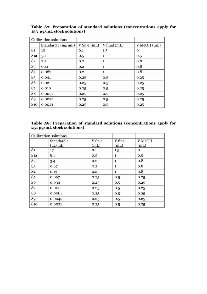
Table A7: Preparation of standard solutions (concentrations apply for 153 µg/mL stock solutions)

Calibration solutions

Standard c (µg/mL) V Sn-1 (mL) V final (mL) V MeOH (mL)

S1 10 0.1 1.5 0

S1a 5.1 0.5 1 0.5

S2 2.1 0.2 1 0.8

S3 0.41 0.2 1 0.8

S4 0.082 0.2 1 0.8

S5 0.041 0.25 0.5 0.25

S6 0.021 0.25 0.5 0.25

S7 0.010 0.25 0.5 0.25

S8 0.0051 0.25 0.5 0.25

S9 0.0026 0.25 0.5 0.25

S10 0.0013 0.25 0.5 0.25

Table A8: Preparation of standard solutions (concentrations apply for 251 µg/mL stock solutions)

Calibration solutions

Standard c (µg/mL)

V Sn-1 (mL)

V final (mL)

V MeOH (mL)

S1 17 0.1 1.5 0

S1a 8.4 0.5 1 0.5

S2 3.4 0.2 1 0.8

S3 0.67 0.2 1 0.8

S4 0.13 0.2 1 0.8

S5 0.067 0.25 0.5 0.25

S6 0.034 0.25 0.5 0.25

S7 0.017 0.25 0.5 0.25

S8 0.0084 0.25 0.5 0.25

S9 0.0042 0.25 0.5 0.25

S10 0.0021 0.25 0.5 0.25

Table A9: Preparation of standard solutions (concentrations apply for 83 µg/mL stock solutions)

Calibration solutions

Standard c (µg/mL)

V Sn-1 (mL)

V final (mL)

V MeOH (mL)

S1 5.6 0.1 1.5 0

S1a 2.8 0.5 1 0.5

S2 1.1 0.2 1 0.8

S3 0.22 0.2 1 0.8

S4 0.044 0.2 1 0.8

S5 0.022 0.25 0.5 0.25

S6 0.011 0.25 0.5 0.25

S7 0.0056 0.25 0.5 0.25

S8 0.0028 0.25 0.5 0.25

S9 0.0014 0.25 0.5 0.25

S10 0.00069 0.25 0.5 0.25

Table A10: Preparation of standard solutions (concentrations apply for 125 µg/mL stock solutions)

Calibration solutions

Standard c (µg/mL)

V Sn-1 (mL)

V final (mL) V MeOH (mL)

S1 8.3 0.1 1.5

S1a 4.2 0.5 1 0.5

S2 1.7 0.2 1 0.8

S3 0.33 0.2 1 0.8

S4 0.067 0.2 1 0.8

S5 0.033 0.25 0.5 0.25

S6 0.017 0.25 0.5 0.25

S7 0.0083 0.25 0.5 0.25

S8 0.0042 0.25 0.5 0.25

S9 0.0021 0.25 0.5 0.25

S10 0.0010 0.25 0.5 0.25

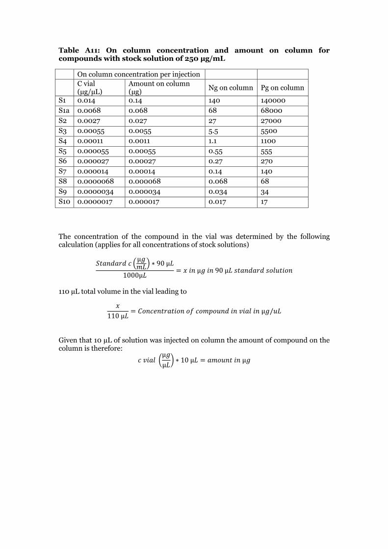
Table A11: On column concentration and amount on column for compounds with stock solution of 250 µg/mL

On column concentration per injection

C vial (µg/µL)

Amount on column (µg)

Ng on column Pg on column

S1 0.014 0.14 140 140000

S1a 0.0068 0.068 68 68000

S2 0.0027 0.027 27 27000

S3 0.00055 0.0055 5.5 5500

S4 0.00011 0.0011 1.1 1100

S5 0.000055 0.00055 0.55 555

S6 0.000027 0.00027 0.27 270

S7 0.000014 0.00014 0.14 140

S8 0.0000068 0.000068 0.068 68

S9 0.0000034 0.000034 0.034 34

S10 0.0000017 0.000017 0.017 17

The concentration of the compound in the vial was determined by the following calculation (applies for all concentrations of stock solutions)

110 µL total volume in the vial leading to

Given that 10 µL of solution was injected on column the amount of compound on the column is therefore:

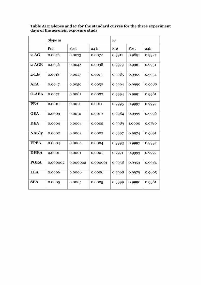
Table A12: Slopes and R2 for the standard curves for the three experiment days of the acrolein exposure study

Slope m R2

Pre Post 24 h Pre Post 24h

2-AG 0.0076 0.0073 0.0072 0.9911 0.9891 0.9927

2-AGE 0.0056 0.0048 0.0038 0.9979 0.9961 0.9931

2-LG 0.0018 0.0017 0.0015 0.9985 0.9909 0.9954

AEA 0.0047 0.0050 0.0050 0.9994 0.9990 0.9980

O-AEA 0.0077 0.0081 0.0082 0.9994 0.9991 0.9981

PEA 0.0010 0.0011 0.0011 0.9995 0.9997 0.9997

OEA 0.0009 0.0010 0.0010 0.9984 0.9999 0.9996

DEA 0.0004 0.0004 0.0005 0.9989 1.0000 0.9780

NAGly 0.0002 0.0002 0.0002 0.9997 0.9974 0.9891

EPEA 0.0004 0.0004 0.0004 0.9993 0.9997 0.9997

DHEA 0.0001 0.0001 0.0001 0.9971 0.9993 0.9997

POEA 0.000002 0.000002 0.000001 0.9958 0.9953 0.9984

LEA 0.0006 0.0006 0.0006 0.9968 0.9979 0.9605

SEA 0.0005 0.0005 0.0005 0.9999 0.9990 0.9981

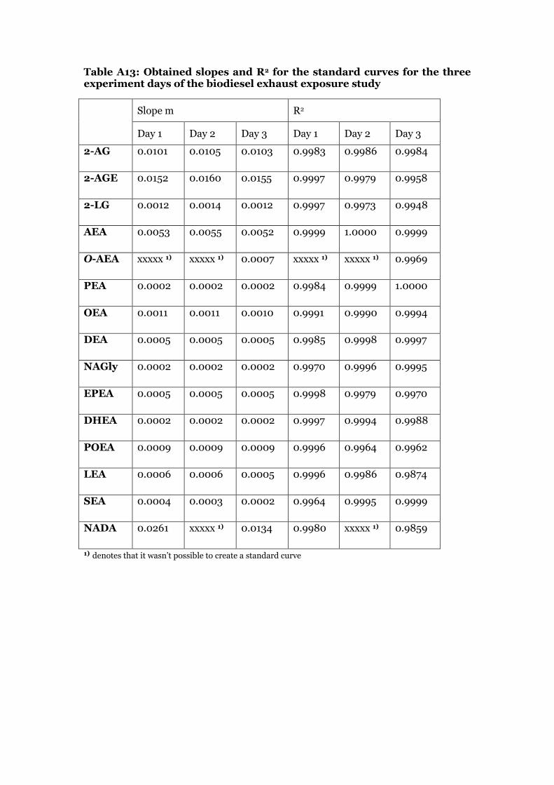
Table A13: Obtained slopes and R2 for the standard curves for the three experiment days of the biodiesel exhaust exposure study

Slope m R2

Day 1 Day 2 Day 3 Day 1 Day 2 Day 3

2-AG 0.0101 0.0105 0.0103 0.9983 0.9986 0.9984

2-AGE 0.0152 0.0160 0.0155 0.9997 0.9979 0.9958

2-LG 0.0012 0.0014 0.0012 0.9997 0.9973 0.9948

AEA 0.0053 0.0055 0.0052 0.9999 1.0000 0.9999

O-AEA xxxxx 1) xxxxx 1) 0.0007 xxxxx 1) xxxxx 1) 0.9969

PEA 0.0002 0.0002 0.0002 0.9984 0.9999 1.0000

OEA 0.0011 0.0011 0.0010 0.9991 0.9990 0.9994

DEA 0.0005 0.0005 0.0005 0.9985 0.9998 0.9997

NAGly 0.0002 0.0002 0.0002 0.9970 0.9996 0.9995

EPEA 0.0005 0.0005 0.0005 0.9998 0.9979 0.9970

DHEA 0.0002 0.0002 0.0002 0.9997 0.9994 0.9988

POEA 0.0009 0.0009 0.0009 0.9996 0.9964 0.9962

LEA 0.0006 0.0006 0.0005 0.9996 0.9986 0.9874

SEA 0.0004 0.0003 0.0002 0.9964 0.9995 0.9999

NADA 0.0261 xxxxx 1) 0.0134 0.9980 xxxxx 1) 0.9859

1) denotes that it wasn’t possible to create a standard curve

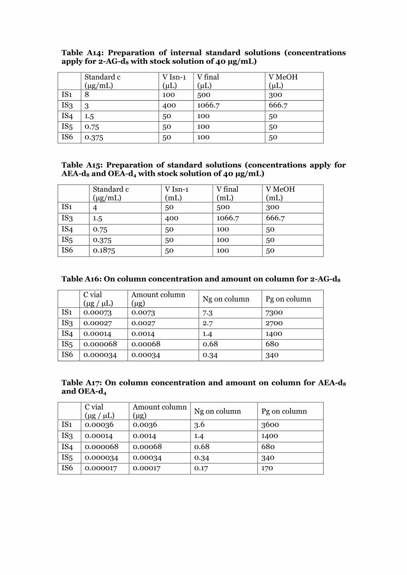
Table A14: Preparation of internal standard solutions (concentrations apply for 2-AG-d8 with stock solution of 40 µg/mL)

Standard c (µg/mL)

V Isn-1 (µL)

V final (µL)

V MeOH (µL)

IS1 8 100 500 300

IS3 3 400 1066.7 666.7

IS4 1.5 50 100 50

IS5 0.75 50 100 50

IS6 0.375 50 100 50

Table A15: Preparation of standard solutions (concentrations apply for AEA-d8 and OEA-d4 with stock solution of 40 µg/mL)

Standard c (µg/mL)

V Isn-1 (mL)

V final (mL)

V MeOH (mL)

IS1 4 50 500 300

IS3 1.5 400 1066.7 666.7

IS4 0.75 50 100 50

IS5 0.375 50 100 50

IS6 0.1875 50 100 50

Table A16: On column concentration and amount on column for 2-AG-d8

C vial (µg / µL)

Amount column (µg)

Ng on column Pg on column

IS1 0.00073 0.0073 7.3 7300

IS3 0.00027 0.0027 2.7 2700

IS4 0.00014 0.0014 1.4 1400

IS5 0.000068 0.00068 0.68 680

IS6 0.000034 0.00034 0.34 340

Table A17: On column concentration and amount on column for AEA-d8 and OEA-d4

C vial (µg / µL)

Amount column (µg)

Ng on column Pg on column

IS1 0.00036 0.0036 3.6 3600

IS3 0.00014 0.0014 1.4 1400

IS4 0.000068 0.00068 0.68 680

IS5 0.000034 0.00034 0.34 340

IS6 0.000017 0.00017 0.17 170

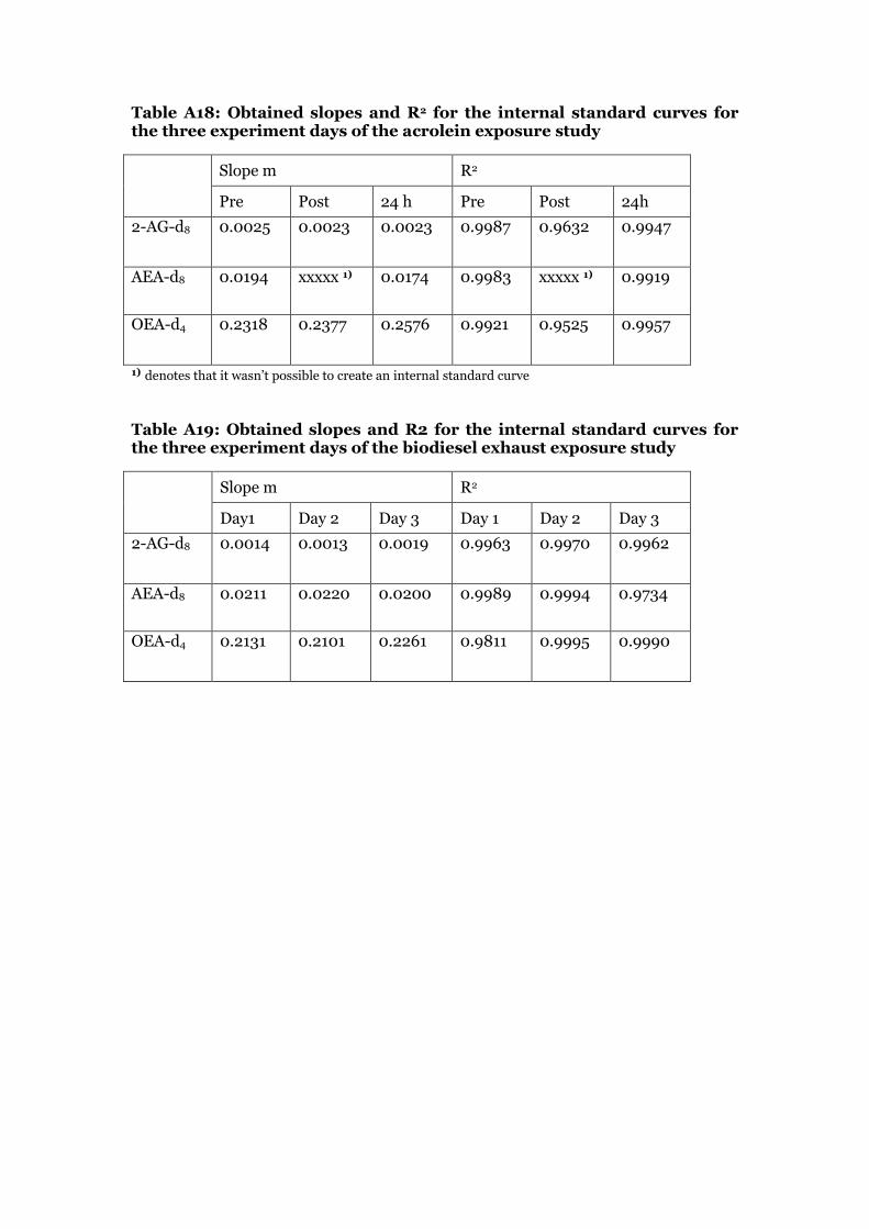
Table A18: Obtained slopes and R2 for the internal standard curves for the three experiment days of the acrolein exposure study

Slope m R2

Pre Post 24 h Pre Post 24h

2-AG-d8 0.0025 0.0023 0.0023 0.9987 0.9632 0.9947

AEA-d8 0.0194 xxxxx 1) 0.0174 0.9983 xxxxx 1) 0.9919

OEA-d4 0.2318 0.2377 0.2576 0.9921 0.9525 0.9957

1) denotes that it wasn’t possible to create an internal standard curve

Table A19: Obtained slopes and R2 for the internal standard curves for the three experiment days of the biodiesel exhaust exposure study

Slope m R2

Day1 Day 2 Day 3 Day 1 Day 2 Day 3

2-AG-d8 0.0014 0.0013 0.0019 0.9963 0.9970 0.9962

AEA-d8 0.0211 0.0220 0.0200 0.9989 0.9994 0.9734

OEA-d4 0.2131 0.2101 0.2261 0.9811 0.9995 0.9990

Fig

ur

e A

1:

Po

ste

r p

re

se

nte

d a

t th

e 2

3r

d A

nn

ua

l In

ter

na

tio

na

l C

an

na

bin

oid

Re

se

ar

ch

So

cie

ty S

ym

po

siu

m o

n

the

Ca

nn

ab

ino

ids

in

Va

nc

ou

ve

r,

Ca

na

da

in

Ju

ne

20

13

.

Department of Chemistry

S-901 87 Umeå, Sweden

Telephone +46 90 786 50 00

Text telephone +46 90 786 59 00

www.umu.se