Corporate Finance

Bin Zou

bzou@ualberta.ca

University of Alberta

2010 FallUpdated: February 22, 2015

Contents

Preface I

1 The Corporation 11.1 Organizational Types of Firms . . . . . . . . . . . . . . . . . . 11.2 Goals of the Corporation . . . . . . . . . . . . . . . . . . . . . 3

2 Financial Statement Analysis 42.1 Financial Statement . . . . . . . . . . . . . . . . . . . . . . . 42.2 Balance Sheet . . . . . . . . . . . . . . . . . . . . . . . . . . . 52.3 Income Sheet . . . . . . . . . . . . . . . . . . . . . . . . . . . 7

3 Time Value Mechanics 103.1 Interest Rate . . . . . . . . . . . . . . . . . . . . . . . . . . . 103.2 Arbitrage and the Law of One Price . . . . . . . . . . . . . . . 123.3 Perpetuity and Annuity . . . . . . . . . . . . . . . . . . . . . 13

4 Investment Criteria 174.1 NPV Rule . . . . . . . . . . . . . . . . . . . . . . . . . . . . . 174.2 Alternative Rules . . . . . . . . . . . . . . . . . . . . . . . . . 184.3 Comparison of Investment Opportunities . . . . . . . . . . . . 21

5 Capital Budgeting 235.1 Fundamentals of Capital Budgeting . . . . . . . . . . . . . . . 235.2 Case Study . . . . . . . . . . . . . . . . . . . . . . . . . . . . 26

6 Bond and Stock Valuations 306.1 Valuing Bonds . . . . . . . . . . . . . . . . . . . . . . . . . . . 306.2 Valuing Stocks . . . . . . . . . . . . . . . . . . . . . . . . . . 34

6.2.1 Dividend-Discount Method . . . . . . . . . . . . . . . . 34

i

ii CONTENTS

6.2.2 Comparison Method . . . . . . . . . . . . . . . . . . . 37

7 Options 397.1 Introduction . . . . . . . . . . . . . . . . . . . . . . . . . . . . 397.2 Properties of Stock Options . . . . . . . . . . . . . . . . . . . 41

7.2.1 Factors Affecting Option Prices . . . . . . . . . . . . . 417.2.2 Bounds for Option Prices . . . . . . . . . . . . . . . . 427.2.3 Put-Call Parity . . . . . . . . . . . . . . . . . . . . . . 45

7.3 The Binomial Pricing Model . . . . . . . . . . . . . . . . . . . 477.4 Black-Scholes Model . . . . . . . . . . . . . . . . . . . . . . . 52

8 Risk and Return 558.1 Statistics Background . . . . . . . . . . . . . . . . . . . . . . . 558.2 Measures of Risk and Return . . . . . . . . . . . . . . . . . . 588.3 Portfolio Return and Risk . . . . . . . . . . . . . . . . . . . . 60

9 Capital Asset Pricing Model and Portfolio Management 629.1 Intuitive View of CAPM . . . . . . . . . . . . . . . . . . . . . 629.2 Portfolio Management . . . . . . . . . . . . . . . . . . . . . . 63

9.2.1 Portfolio Selection without Risk-free Asset . . . . . . . 649.2.2 Portfolio Selection with Risk-free Asset . . . . . . . . . 68

9.3 Mathematical Proof of CAPM . . . . . . . . . . . . . . . . . . 71

Preface

Those notes on Corporate Finance are mainly based on the lectures of FIN501 taught by Professor Andras Marosi in Fall 2010 at the University of Al-berta, and the reference book Corporate Finance (Canadian Edition) writtenby Jonathan Berk, Peter DeMarzo and David Stangeland [1].

If you find any typos or problems in the notes, please let me know by email.

I

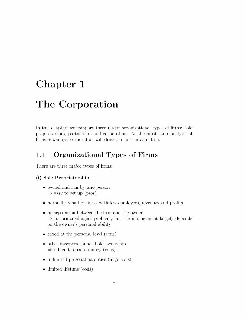
Chapter 1

The Corporation

In this chapter, we compare three major organizational types of firms: soleproprietorship, partnership and corporation. As the most common type offirms nowadays, corporation will draw our further attention.

1.1 Organizational Types of Firms

There are three major types of firms:

(i) Sole Proprietorship

• owned and run by one person⇒ easy to set up (pros)

• normally, small business with few employees, revenues and profits

• no separation between the firm and the owner⇒ no principal-agent problem, but the management largely dependson the owner’s personal ability

• taxed at the personal level (cons)

• other investors cannot hold ownership⇒ difficult to raise money (cons)

• unlimited personal liabilities (huge cons)

• limited lifetime (cons)

1

2 1. The Corporation

• hard to transfer ownership (cons)

(ii) Partnership

• like an extension of sole proprietorship with more than one owner

• taxed at the personal level (cons)

• all partners are liable for the firm’s debt (huge cons)

• Special case–limited partnership: at least one general partner withunlimited liabilities and several partners who have limited liabilities totheir investment but has no authorities on management

• limited lifetime (cons)

• hard to transfer ownership (cons)

(iii) Corporation

• legally defined and separate from the owners

• only responsible for its own obligations⇒ owners have limited liabilities (pros)

• articles of incorporations (or corporate charters) which stipulate theownership, existence and other regulations of the corporation (possiblecons)

• no limit on the number of owners, and ownership is easy to transfer(big pros)

• all the owners (stockholders, equity holders) have the right to sharedividend according to their investment proportions (pros)

• all the owners are entitled to vote for firm’s decisions with differentweights (pros)

• no special expertise is required to be an owner⇒ easy to accumulate money (big pros)

• double taxation–the corporation pays tax on its profits and the share-holders pay their personal income tax

1.2. Goals of the Corporation 3

Compensation for double taxation in Canada: income trusts which comein three forms–business income trust, energy trust and real estate investmenttrust (REIT). In those firms, no corporate tax is collected. (However, thefirst two trusts will not exist anymore after 2011 in Canada.)

1.2 Goals of the Corporation

A common goal of corporation is to maximize shareholders’ wealth, espe-cially, in Canada, the United States and the UK. While in Japan and someEuropean countries, corporations try to increase stakeholders’ satisfaction(The stakeholders of a corporation include its shareholders, debt holders, cus-tomers, suppliers, communities and the government). Other possible choicesinclude maximizing sales/profit and maintaining steady growth.

The separation of ownership and management in a corporation may leadto principal-agent problems in which the managers don’t pursue the maxi-mization of shareholders’ profits.

Case. Liquor Barn Income Fund, a publicly traded company, used toown and operate liquor stores in Alberta. Liquor Barn had an agreementwith Devco: Devco would purchase individual liquor stores and later resellthem to Liquor Barn. In this case, the CEO of Liquor Barn was the ownerof Devco and therefore as CEO, he should buy liquor stores as cheaply aspossible; however, as the owner of Devco, he had an interest to ask a highprice when Devco sold stores to Liquor Barn. Finally, Liquor Stores IncomeFund, a competing firm, made an offer to purchase all Liquor Barn shares(at a premium) and Liquor Barn shareholders eventually accepted.

Corporate control to address principal-agent problem

• minimize the number of interest-conflict decisions

• fire managers when they don’t work well

• takeover (to replace the board of directions and the CEO)

Chapter 2

Financial Statement Analysis

From the results in Chapter 1, we know that one advantage of corporationis that it can have many owners, especially shareholders. Therefore, finan-cial managers and owners need to assess their companies’ performance whileinvestors also want to estimate the firms’ performance to decide whether tobuy or sell the firms’ stocks. A good way for all of them to evaluate the firms’performance is through their financial statements. In this chapter, we discusstwo major financial statements: the balance sheet and the income sheet, andstudy how to use these statements to evaluate a company’s performance.

2.1 Financial Statement

Financial statements are accounting reports with past performance informa-tion that a firm publishes periodically. Financial statements of Canadiancompanies can be found on the website of the System for Electronic Docu-ment Analysis and Retrieval (SEDAR www.sedar.com). Generally AcceptedAccounting Principles (GAAP) provide a common set of rules and a standardformat for public companies to prepare financial statements. In order to en-sure the accuracy of financial statements, a neutral third party, known as anauditor, is usually involved. According to International Financial ReportingStandards (IFRS), every public company is required to produce five financialstatements: the balance sheet, the income sheet, the statement of cash flows,the statement of shareholders’ equity and the statement of comprehensiveincome.

4

2.2. Balance Sheet 5

2.2 Balance Sheet

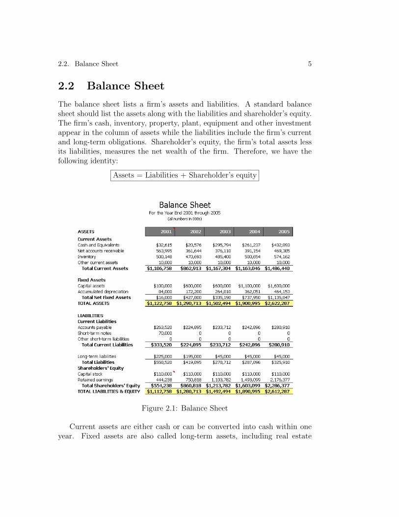
The balance sheet lists a firm’s assets and liabilities. A standard balancesheet should list the assets along with the liabilities and shareholder’s equity.The firm’s cash, inventory, property, plant, equipment and other investmentappear in the column of assets while the liabilities include the firm’s currentand long-term obligations. Shareholder’s equity, the firm’s total assets lessits liabilities, measures the net wealth of the firm. Therefore, we have thefollowing identity:

Assets = Liabilities + Shareholder’s equity

Figure 2.1: Balance Sheet

Current assets are either cash or can be converted into cash within oneyear. Fixed assets are also called long-term assets, including real estate

6 2. Financial Statement Analysis

and equipment. Depreciation is not an actual cash expense but is markedto recognize the fact that some assets like buildings become less valuable.The book value of an asset is the difference between its acquisition cost andaccumulated depreciation.

Liabilities that need to be paid off within one year are called currentliabilities. Those liabilities with maturity longer than one year are long-termliabilities. One of the current liabilities is accounts payable, the amountsowned to suppliers for products or service purchased with credits.

Shareholder’s equity is also known as the book value of equity, however,it is not an accurate measurement of the firm’s true value. For instance, thecurrent value of the firm’s land may be higher than its original acquisitionvalue. Besides, there are other factors which play an important role in de-termining a firm’s value, such as expertise of the firm’s employees, and thefirm’s reputation in the industry. The total market value of a firm’s equityequals the market price per share times the number of shares, referred to asthe company’s market capitalization, which indicates investors’ expectationin the future.

The liquidation value of the firm is the value that would be left if itsassets were sold and liabilities paid. From the balance sheet, we can obtainan estimate of the liquidation value.

Market-to-Book Ratio (Price-to-Book [P/B] Ratio)

Market-to-Book Ratio =Market Value of Equity

Book Value of Equity

Most successful companies have market-to-book ratio greater than 1,meaning that the value of firm’s assets can produce more than their his-torical cost (or liquidation value). Normally, a higher market-to-book ratiois a good sign of the firm’s future performance.

Debt-Equity Ratio

Debt-Equity Ratio =Total Debt

Total Equity

The debt-equity ratio is always used to assess a firm’s leverage. In theabove formula, we can use either book or market values for debt and equity to

2.3. Income Sheet 7

calculate this ratio. Since the book value of the firm’s equity is not a preciseassessment, so it’s better to use market value of its equity for calculation.However, as the difference between the book value of debt and the marketvalue of debt is basically slight, we always ignore such difference in practice.

Enterprise Value

Enterprise Value=Market Value of Equity + Debt - Cash

The enterprise value of a firm assesses the value of the underlying busi-ness assets, also can be interpreted as the net cost to take over the business.

Problem 2.1. On December 31, 2007, Maple Leaf Foods inc. (MFC) hada share price of $14.85, 129.6 million shares outstanding, a market-to-bookratio of 1.66, a book debt-equity ratio of 0.76, and cash of $28 million. Whatwas Maple Leaf’s market capitalization? What was its enterprise value?

Solution. Its market capitalization is $14.85 per share × 129.6 millionshares= $1.92 billion. From its market-to-book ratio, we can obtain MapleLeaf’s book value of equity, 1.92/1.66 = $1.16 billion. Then its total debt canbe calculated as 0.76 × 1.16 = $0.88 billion. Lastly, we calculate the MapleLeaf’s enterprise value, 1.92 + 0.88− 0.028 = $2.77 billion.

2.3 Income Sheet

The income sheet, also called statement of earnings, statement of operations,or profit and loss (“P & L”) statement, lists a firm’s revenues and expensesover a period of time. The net income line of the income statement showsthe firm’s profitability during that period.

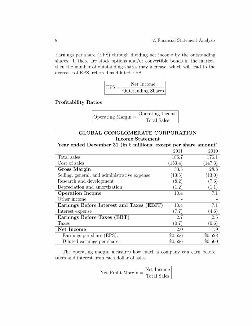
Gross margin is the difference between the first two items, total sales andcost of sales. The following three items comprise operation expenses. Thefirm’s gross margin less the operation expenses is called operating income.Other income lists all the other cash flows obtained from non-central part ofthe firm’s business, like profits from financial investment. Earnings BeforeInterest and Taxes (EBIT) is the summation of operating income and otherincome. After deducting the interest paid on outstanding debt (Interestexpense), we obtain Earnings Before Taxes (EBT), and then we subtractcorporate taxes from EBT to obtain the firm’s net income. We calculate

8 2. Financial Statement Analysis

Earnings per share (EPS) through dividing net income by the outstandingshares. If there are stock options and/or convertible bonds in the market,then the number of outstanding shares may increase, which will lead to thedecrease of EPS, referred as diluted EPS.

EPS =Net Income

Outstanding Shares

Profitability Ratios

Operating Margin =Operating Income

Total Sales

GLOBAL CONGLOMERATE CORPORATIONIncome Statement

Year ended December 31 (in $ millions, except per share amount)2011 2010

Total sales 186.7 176.1Cost of sales (153.4) (147.3)Gross Margin 33.3 28.8Selling, general, and administrative expense (13.5) (13.0)Research and development (8.2) (7.6)Depreciation and amortization (1.2) (1.1)Operation Income 10.4 7.1Other income - -Earnings Before Interest and Taxes (EBIT) 10.4 7.1Interest expense (7.7) (4.6)Earnings Before Taxes (EBT) 2.7 2.5Taxes (0.7) (0.6)Net Income 2.0 1.9

Earnings per share (EPS): $0.556 $0.528Diluted earnings per share: $0.526 $0.500

The operating margin measures how much a company can earn beforetaxes and interest from each dollar of sales.

Net Profit Margin =Net Income

Total Sales

2.3. Income Sheet 9

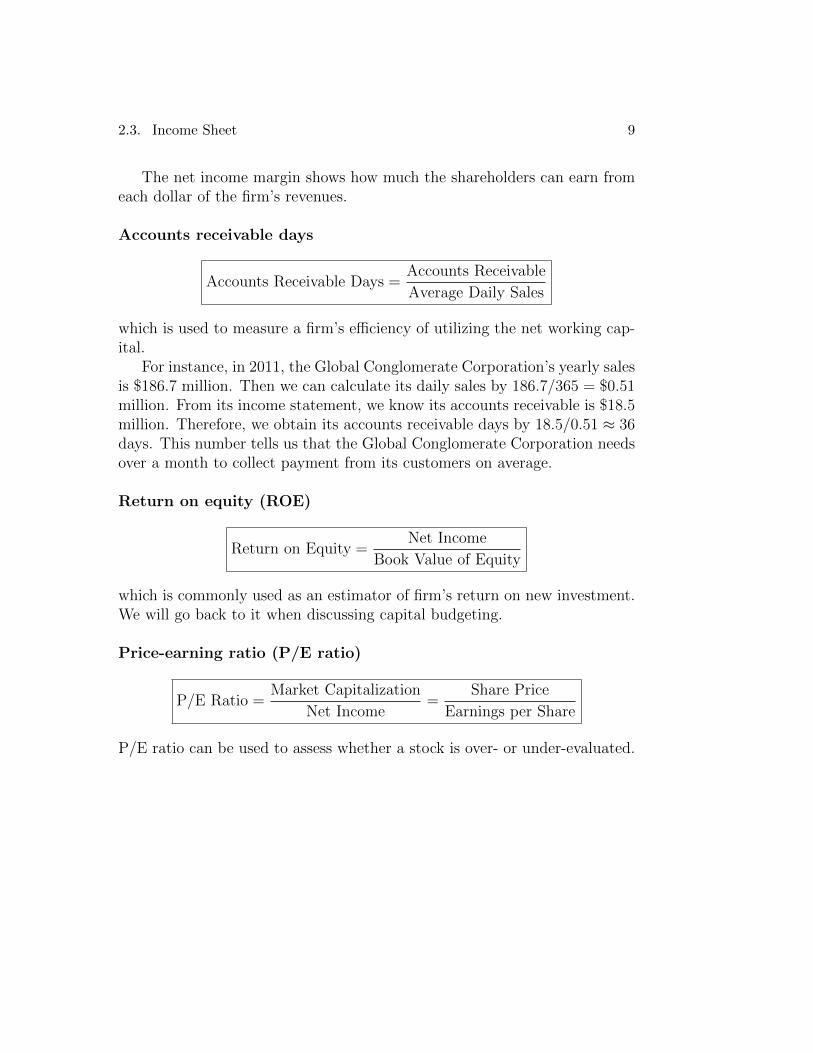
The net income margin shows how much the shareholders can earn fromeach dollar of the firm’s revenues.

Accounts receivable days

Accounts Receivable Days =Accounts Receivable

Average Daily Sales

which is used to measure a firm’s efficiency of utilizing the net working cap-ital.

For instance, in 2011, the Global Conglomerate Corporation’s yearly salesis $186.7 million. Then we can calculate its daily sales by 186.7/365 = $0.51million. From its income statement, we know its accounts receivable is $18.5million. Therefore, we obtain its accounts receivable days by 18.5/0.51 ≈ 36days. This number tells us that the Global Conglomerate Corporation needsover a month to collect payment from its customers on average.

Return on equity (ROE)

Return on Equity =Net Income

Book Value of Equity

which is commonly used as an estimator of firm’s return on new investment.We will go back to it when discussing capital budgeting.

Price-earning ratio (P/E ratio)

P/E Ratio =Market Capitalization

Net Income=

Share Price

Earnings per Share

P/E ratio can be used to assess whether a stock is over- or under-evaluated.

Chapter 3

Time Value Mechanics

In this chapter, we will introduce the time value of money and show how todiscount and compound the value among different time points. By the argu-ment of no-arbitrage theory, we will deduce an important principle: law ofone price. Then we shall use this principle to price annuities and perpetuities.

3.1 Interest Rate

For most financial decisions, incomes and expenditures occur at differenttime. Generally speaking, a certain amount of money at present time shouldworth more than the same amount in the future. Such difference in valuebetween different time is referred as time value of money. Hence we shoulddiscount or compound values to the same time in order to compare them.The rate we use for discounting or compounding through different time isinterest rate.

For simplicity, let’s consider a discrete time model, in which time is num-bered by natural numbers 1, 2, · · · . Let r be the risk-free interest rate, forinstance, we can use three-month treasury rate as a replacement in practice.Therefore, future value is obtained by

Pt = Pt−1 · (1 + r) = P0 · (1 + r)t, 1 ≤ t ∈ N+. (3.1)

By the same token, we can also discount value from future time t to curren-t/past time s (s < t) by dividing interest rate correspondingly.

Notice that the above formula assumes that all the gained interest will bere-invested in the same asset P . So rate r is actually the compound interest

10

3.1. Interest Rate 11

rate. Alternatively, we have simple rate, and using simple interest rate r,future value is calculated by

Pt = P0 · (1 + rt). (3.2)

In the above discussion, we have the same time interval (time unit) andr is actually the interest rate of one period. However, if we have differentscales, for instance, annual rate ra, semi-annual rate rs, quarterly rate rq,monthly rate rm, weekly rate rw and daily rate rd, then we need to find therelationship among them. If we assume there are 365 days per year, then wecan convert rd into ra by

ra = (1 + rd)365 − 1. (3.3)

In general case, assume that ri and rj are two interest rates of time length iand j, and i = N · j. For instance, in the previous example, period i is oneyear while period j is one day, so N = 365. Then we shall have:

ri = (1 + rj)N − 1. (3.4)

Notice that all the above mentioned compound interest rates are effectiverates. However, most quoted interest rates (the ones you can find throughbanks) are not effective rates. For instance, a commonly used one is annualpercentage rate (APR), which is the amount of simple interest earned inone year. In order to convert the APR to effective annual rate (EAR),we need to know the compounding times per year.

Example. Bank of Montreal issues a security with interest rate of 5%per year with monthly compounding, then the EAR of this security is givenby:

EAR =

(1 +

APR

12

)12

− 1 = 5.12%.

Given APR with K compounding periods per year, the effective interest rateper compounding period rp is:

rp =APR

K(3.5)

while the EAR is simply:

EAR =

(1 +

APR

K

)K

− 1 = (1 + rp)K − 1. (3.6)

12 3. Time Value Mechanics

Many loans, such as consumer loan and car loans, have monthly paymentsand are quoted in APR with monthly compounding. This type of loansis known as amortizing loans because in each payment, you pay bothprincipal and interest. However, in Canada, home mortgage is quoted inAPR with semiannual compounding but have monthly payments. Therefore,the effective monthly rate rm is calculated as

rm =

(1 +

APR

2

)1/6

− 1. (3.7)

In (3.6), when K → ∞, 1+EAR will converge to eAPR, which is corre-sponding to continuous models. So if compounding happens at every pointin time axis (verbal explanation of continuous model), then if we deposit 1$dollar today, we will get eAPR dollars one year later.

So far, all the interest rates we have discussed before so-called nominalinterest rates, which indicates how much money you will earn by investingin a saving account (other security with certain return) for a certain period.But in real life, there is inflation/deflation which will alter the purchasingvalue of money. The interest rate after adjusting for inflation reflects thereal change of purchasing power of your money, and this rate is called realinterest rate. Let i be the inflation rate and r be the nominal interest rate,then real interest rate rr is determined by (all rates are quoted in same timeperiod.)

1 + rr =1 + r

1 + i. (3.8)

An approximation is given by

rr ≈ r − i. (3.9)

3.2 Arbitrage and the Law of One Price

Arbitrage is an investment portfolio which can guarantee positive profitsfor sure, or mathematically defined as

V (0) = 0, V (1) ≥ 0 and P (V (1) > 0) > 0, (3.10)

where V (t) denotes the value of the portfolio at time t and P is the actualprobability measure.

3.3. Perpetuity and Annuity 13

By the definition of arbitrage, it can be considered as “free-lunch”, and allrational investors will buy arbitrage portfolios as much as they could. Thosetrading activities will for sure drive up the prices of the arbitrage portfolios,which will ultimately cause the arbitrage opportunities to vanish. Based onsuch argument, we can assume that an efficient market is arbitrage-free.

Remark. It can be shown the sufficient and necessary condition for a marketto be arbitrage-free is that there exists at least one risk-neutral probabilitymeasure P ∗. Under this probability measure P ∗, all assets have the samereturn as the risk-free asset and so bear the same risk, which is the reasonwhy this probability measure is called risk-neutral. For further reference,please read [10].

Law of one price. If an investment opportunity is traded simultaneouslyin different competitive markets, then the price is the same in all markets.

According to the law of one price, for any security with certain future priceS(1), its present price S(0) is determined by S(0) = S(1)/(1 + r), where ris the risk-free rate. Or equivalently, we can say that financial investmentdoesn’t increase or decrease any extra value. (Such conclusion is made underthe assumption that there is no risk/uncertainty) This conclusion is knownas Separation principle, which gives the reason for raising capital throughissuing stocks or bonds.

3.3 Perpetuity and Annuity

A perpetuity is a stream of cash flows Cn that occur at regular intervalsand last forever. The real-life example is British government bond (calledconsol bond). Normally, when taking about perpetuity, we assume that allCn are equal, denoted by C. Suppose that the cash flows start from time 1and the risk-free interest rate in the same time interval is denoted by r (suchassumption will hold unless otherwise specified, for instance, the staring pointwill be 0 only when we consider perpetuity/annuity due). Therefore, we can

14 3. Time Value Mechanics

calculate the present value of such defined perpetuity:

PV =C

1 + r+

C

(1 + r)2+

C

(1 + r)3+ · · · =

∞∑t=1

C

(1 + r)t

=C

1 + r· 1

1− 1

1 + r

=C

r. (3.11)

For a perpetuity with payment beginning at time 0, we call it perpetuitydue. If we still use (3.11), then we will obtain the value of perpetuity due attime −1, so to calculate its present value (at time 0), we need to accumulateto time 0 by multiplying 1 + r, thus the present value of a perpetuity due is:

PV =C(1 + r)

r. (3.12)

A growing perpetuity is a perpetuity with growing cash flows at growthrate g, so Cn = C1(1 + g)t−1, t ≥ 1.

• r > gUnder the same assumption, the present value of growing perpetuitycan be calculated as follows:

PV =C1

1 + r+

C2

(1 + r)2+

C3

(1 + r)3+ · · · = C1

1 + g

∞∑t=1

(1 + g)t

(1 + r)t

=C1

1 + g·

1 + g

1 + r

1− 1 + g

1 + r

=C1

r − g. (3.13)

• r ≤ gThe convergence radius of infinite power series is 1 and it is evidentthat the power series doesn’t converge at point 1. According to thisproposition, it’s easy to see that in this case the growing perpetuityhas a infinite large present value.

3.3. Perpetuity and Annuity 15

An annuity is a stream of N equal payments that occur at regular timeintervals. Using the same method, its present value is given by

PV =C

1 + r+

C

(1 + r)2+ · · ·+ C

(1 + r)N=

N∑t=1

C

(1 + r)t

=C

1 + r·

1− 1

(1 + r)N

1− 1

1 + r

=C

r·(

1− 1

(1 + r)N

). (3.14)

Correspondingly, we also have growing annuity and its present valuecan be obtained according to two different cases:

• r = g

PV =C1

1 + r

N−1∑t=0

(1 + g

1 + r

)t

=N C1

1 + r. (3.15)

• r 6= g

PV =C1

1 + r+

C2

(1 + r)2+ · · ·+ CN

(1 + r)N=

C1

1 + r

N−1∑t=0

(1 + g

1 + r

)t

=C1

1 + r·

1−(

1 + g

1 + r

)N

1− 1 + g

1 + r

=C1

r − g

[1−

(1 + g

1 + r

)N]. (3.16)

Example. Your six years old wants to go to Princeton. This will costyou $30, 000 per year for 4 years. On her next birthday you will start to putmoney into an account paying 14% annual rate and continue to deposit thesame amount every year until her 17th birthday. The first tuition paymentwill occur on her 18th birthday, the second on her 19th birthday, etc. Howmuch do you need to deposit to this account every year?

Solution. In this example, we have two annuities, the first one will lastfrom time 1 to 11 with payment C (the value we need to calculate) whilethe second will begin at time 12 and end at time 15 with payment $30, 000,where we label 6th birthday as time 0 and time interval is one year. Since

16 3. Time Value Mechanics

we use the first annuity to finance the second one, so obviously, their valueshould coincide at any time. Firstly, by (3.14), we can get the value of secondannuity at time 11:

P 211 = 30000×

[1

0.14

(1− 1

(1.14)4

)]= $87, 411.37.

Therefore, by discounting, we can calculate its present value:

P 20 =

P 211

(1.14)11= $20, 683.05.

According to the above argument, we know that the first annuity should alsohave the same present value of $20, 683.05, and so

P 10 = C ×

[1

0.14

(1− 1

(1.14)11

)]= $20, 683.05.

⇒ C = $3, 793.15.

Chapter 4

Investment Criteria

In corporate finance, one of the most important topics is to study the invest-ment decision rules. Among all these rules, net present value (NPV) isthe most widely used one while there are also some other alternative rulescommonly used in real industries like the payback investment rule. Inthis chapter, we will discuss major decision rules in details.

Before we introduce decision rules, we should answer a question first:what should a good criterion do? Basically, a good evaluation should

• Consider all cash flows

• Account for time differences

• Provide unambiguous decision

• Measure wealth created for shareholders

4.1 NPV Rule

When the payoff of an investment is discounted back to present time, thensuch discounted value is called present value. Then we can define netpresent value of an investment as:

NPV = PV(Benefits) - PV(Costs).

If an investment opportunity has a strictly positive NPV, then such in-vestment can generate profits and thus should be taken. In addition, if there

17

18 4. Investment Criteria

are several investment opportunities which generate positive NPV, then weshould take the one with the highest NPV. These arguments then lead to thefamous NPV rule: When making investment decision, take the alternativeone with the highest positive NPV.

Notice that if there are many options, we cannot just take the one withthe highest NPV. Because it is possible that even the highest one is negative,then we should reject all these options.

For instance, consider a project with C0 outlay instantly and cash flowsCt, 1 ≤ t ≤ T . Assume the cost of capital is r, then the NPV of this projectis:

NPV = −C0 +T∑t=1

Ct

(1 + r)t.

Define the profitability index of a project by

PI =PV

I0

, (4.1)

where PV is the present value of all the benefits of the project and I0 is thepresent value of all the cost of the project.

Since PI > 1⇔ NPV > 0, we should take the project when its PI > 1.

Internal rate of return (IRR) is the interest rate which makes the N-PV of a project equal to zero. When making decisions, we need to know thecost of capital, but we can only estimate this rate, thus IRR can be usedto measure the sensitivity of our estimation. In order to make the correctdecision, the biggest error of estimating the cost of capital is the differencebetween the cost of capital and IRR.

4.2 Alternative Rules

The Payback Rule

To use the payback rule, we need to calculate the payback period (Tp) ofa project and then compare the payback period with the pre-specified timeperiod (Ts). If Tp < Ts, then we accept the project.

Example. Assume that we will accept the project when its payback periodis less than 5 years. Consider a project with investment C0 = $200 million

4.2. Alternative Rules 19

and positive cash flows Ci = $50 million in year i, 1 ≤ i ≤ 6. Should weaccept this project?

Solution. To fully pay back the initial investment, we need C0/Ci = 4years. Since the payback period of this project is less than 5, so we shouldlaunch this project.

From the above example, we can easily see that the payback rules doesn’tconsider the time value of money and thus it is not a reliable rule. Tomake the payback rule more reasonable, we can use discounted cash flows tocalculate the payback rule.

Example continued. In the previous example, suppose cost of capitalis r = 10%. Then we discount all the cash flows to the present time and willobtain:

C1 = $45.45, C2 = $41.32, C3 = $37.57, C4 = $34.15, C5 = $31.05, C6 = $28.22.

Since∑5

t=1 Ct = $189.54 < C0 and∑6

t=1Ct = $217.76 > C0, so in thiscase, the payback period is Tp = 6 > 5. According to the payback rule, weshould turn down this project. But obviously, the NPV of this project is217.76−200 = $17.76 million, and based on NPV rule, we should accept thisproject.

This example tells us that even the modified payback rule is not trustful,and the reason is because the pre-set time period is not entirely objectiveand accurate. However, the most favorable advantage of the payback ruleis simplicity, we even don’t need to know the cost of capital to make thedecision.

The Internal Rate of Return Rule

IRR rule: we should only take the project when its IRR is greater than theproject’s cost of capital. This rule directly comes from the definition of IRR,since IRR is the rate such that NPV=0, so if IRR > r, then we should havepositive NPV if the cash flows are normal. Regarding the term “normal”,we mean the cost occurs right now and benefits come in the future time.Therefore, IRR rule coincides with NPV rule when the cash flows of theproject is normal. However, the above IRR rule will give the reverse resultwhen cash flows are unconventional.

Example. Consider the following two projects: project A requires invest-ment $12, 000 today and will give $15, 600 next year while project B offers

20 4. Investment Criteria

$12, 000 cash right now but needs outlay $15, 600 next year. Then whichproject should we take according to different cost of capital r?

Solution. Firstly, it’s easy to calculate the IRR for two projects andboth of them have the same IRR 30%. We can plot the NPV-r figure for twoprojects and find that their NPV have totally different correlation to the costof capital. From the picture, we know that IRR rule works for project A sincethe NPV of project A is positive when IRR exceeds the cost of capital.

Another problem of IRR rule is that the project may have no IRR or havemore than one IRR.

Economic Value Added Rule

Consider a project with initial cost I dollars today and cash flows Cn in eachperiod n. The economic value added (EVA) in period n is given by

EV An = Cn − rI. (4.2)

If the investment is a changing variable, use In to denote the investmentneeded in period n and Dn represents the depreciation in period n. Then theEVA is defined as

EV An = Cn − rIn−1 −Dn. (4.3)

The EVA rule states that we should accept the project if the sum of presentvalue of all EVAs.

Example. Consider a project with C0 = −$300, 000 and C1 = · · · =C5 = $75, 000. The cost of capital is r = 7% per year and the initial coston equipment will be equally worn out over five years. Should we accept thisproject?

4.3. Comparison of Investment Opportunities 21

Solution. Firstly, it’s easy to identify that Dn = $60, 000 and so In =C0−nDn, 0 ≤ n ≤ 5. Then using EV An = Cn−rIn−1−Dn, we can obtain thestreams of EVAs. For instance, EV A1 = 75, 000− 7%× 300, 000− 60, 000 =−6, 000 and EV A4 = 75, 000− 7%× 120, 000− 60, 000 = 6, 600. Therefore,the sum of present value of all EVAs is given by

PV =−6, 000

1.07+−1, 800

1.072+

2, 400

1.073+

6, 600

1.074+

10, 800

10.075= $7, 510.

So according to EVA rule, we should take this project.

4.3 Comparison of Investment Opportunities

In the above two sections, we only deal with single project problem, “whetherwe should take the project or not?”. But in this section, we face more optionsand need to decide which one to take or turn down all of them. For mutuallyexclusive investment opportunities, we should take the one with the highestpositive NPV and reject all of them if none of them have positive NPV.

Projects with Different Lifetime

In this case, we cannot simply compare the NPV but have to calculate theeffective annual cost, EAC and take the one with the least EAC.

Example. Firm A needs to purchase one machine and has two optionsright now. The information of these two options are listed below:

Machine Initial Outlay Operating Cost per year Lifetime1 10,000 3,000 32 9,000 4,000 5

Which machine should Firm A buy? (Cost of capital is given as r = 10%.)Solution. Firstly, let’s calculate the present value of the cost of two

machines:

PV1 = −10, 000− 3, 000

0.10

(1− 1

1.13

)= −17, 460.55,

PV2 = −9, 000− 4, 000

0.10

(1− 1

1.15

)= −24, 163.47.

22 4. Investment Criteria

If we just consider the PV, then we should choose Machine 1 because of lesscost in total. But we need to notice that PV1 is the present value of costover 3 years while PV2 covers 5 years. So the fair game is to compare theEAC not the total cost. To calculate the EAC for Machine 1, we can use thefollowing formula:

PV1 =C1

0.1

(1− 1

1.13

)⇒ C1 = −7, 021.15.

Similarly, we can also get the EAC of Machine 2 as C2 = −6, 374.17. SinceMachine 2 has the lower EAC, we should purchase Machine 2 instead ofMachine 1.

Projects with Resource Constraints

If there are resource constraints, then NPV rule has to be applied with con-straints. Basically, we rank the projects according to their PI and launch in-teger optimization programming to find the optimal combination of projects.

Example. Assume a firm has $1, 000 cash available and is unable toraise any more capital. Currently, it has several projects available, which arelisted in the following table:

Project Cost PIA 500 2B 800 1.8C 400 1.5

Solution. If we take Project B, the NPV will be (1.8− 1)× 800 = 640.If we take Projects A and C, then what we will get is (2− 1)× 500 + (1.5−1) × 400 = 700. Therefore, under the budget constraint, we should chooseProjects A and C.

Chapter 5

Capital Budgeting

A capital budget lists all the projects that a company plants to take duringthe coming year while the process of constructing capital budget is calledcapital budgeting.

5.1 Fundamentals of Capital Budgeting

Firstly, notice that earnings are accounting concept and different from actu-al cash flow. The incremental earnings are the amount of money expectedto gain as a result of investment. To estimate the incremental earnings, weneed to forecast the revenue and cost. The difference of sales and cost ofgoods sold is gross profit,

Gross Profit=Sales - Cost of Goods Sold.

Generally, operating cost includes advertising, marketing and support costsbut excludes equipment cost. Besides, there might be other costs in theproject like research cost. But among them, there are two special costs: sunkcost and opportunity cost. A sunk cost is any unrecoverable cost whichfirm already paid, hence the firm’s decision won’t make any change to thiscost. For this reason, this cost should be excluded from capital budgeting.The opportunity cost of using a resource is the value it could have provided inits best alternative use. For instance, a company has some spare warehousewhich can be rented out for 1 million per year but it will use the warehouseif it decides to take a certain project. In capital budgeting of this project,

23

24 5. Capital Budgeting

we should include the opportunity cost 1 million because taking this projectwill cost us a loss of 1 million income.

Net Working Capital (NWC) is the difference between current assetsand current liabilities. To better interpret NWC, we introduce the followingterms:

• Receivables collected (RC) VS Sales booked (S)

• Expenses paid (EP) VS Expenses incurred (E)

Apparently, RC 6= S and EP 6= E since the firms cannot get all the moneyof sales immediately and won’t pay all the cost at the same when purchasingthe goods/materials. So we have:

S −RC = ∆AR (Account Receivable)

E − EP = ∆AP (Account Payable)

Then NWC is given by:

NWC = Current Assets− Current Liabilities

= Cash + Inventory + Receivables - Payables (5.1)

Therefore, the change of NWC in year t is

∆NWCt = NWCt −NWCt−1 = ∆ARt + ∆It −∆APt, (5.2)

where we assume there is no change in cash and I stands for inventory. Whenwe sum all ∆NWCt together, we should get zero.

Capital expenditures (CapEx) are the investments in plant, propertyand equipment. They are cash expenses but will not be listed as expens-es when calculating earnings. Instead, such expenditures will be deductedgradually for tax purpose as capital cost allowance (CCA). Assume anasset is in class d and the undepreciated capital cost (UCC) of the assetpool is denoted by UCCt in year t, then CCA in year t is given by:

CCAt = UCCt × d. (5.3)

The formula for calculating UCC is listed as follows:

t = 1 UCC1 = 0.5× CapEx,

t ≥ 2 UCCt = CapEx×(

1− d

2

)× (1− d)t−2, (5.4)

5.1. Fundamentals of Capital Budgeting 25

where the first formula comes from the so-called half-year rule.

Use St denote sales and Et be all the costs except depreciation (CapEx),then the earnings before interest and taxes (EBIT) is:

EBITt = St - Et - CCAt,

and unlevered net income (UNI) (excluding interest expense, so no bor-rowing to finance project) is then given by:

Unlevered Net Income = EBIT ×(1− τc).

To compute free cash flow, we should add CCA back to unlevered netincome (since CCA is not an actual cash flow), subtract actual capital ex-penditure (CapEx) and less the change of NWC. Therefore, free cash flow iscalculated by

CFt = UNIt + CCAt − CapExt −∆NWCt

= (St − Et − CCAt) · (1− τc) + CCAt − CapExt −∆NWCt

= (St − Et)× (1− τc) + CCAt × τc − CapExt −∆NWCt (5.5)

In order to decide whether to take a project, we need to discount all CFt

to present time and add them together to see whether the NPV is greaterthan zero. Thus we need to calculate the present value of all CCA taxshield. To do this, we shall decompose the cash flows of CCA tax shieldsinto two growing perpetuities: the first one starts in year 1 with first cashflow C1 = 0.5 × CapEx × d × τc and growth rate −d while the second oneis same to the first one except starting in year 2. Therefore, we have thepresent value of CCA tax shield:

PV =C1

r + d+

C1

r + d× 1

1 + r

=CapEx× d× τc

r + d×

1 +r

21 + r

(5.6)

Notice that (5.6) only holds when the asset is not sold. If assets are nolonger needed and company decides to sell it in future time year t, then it willgain salvage value (liquidation value). If the assets are sold at a higher

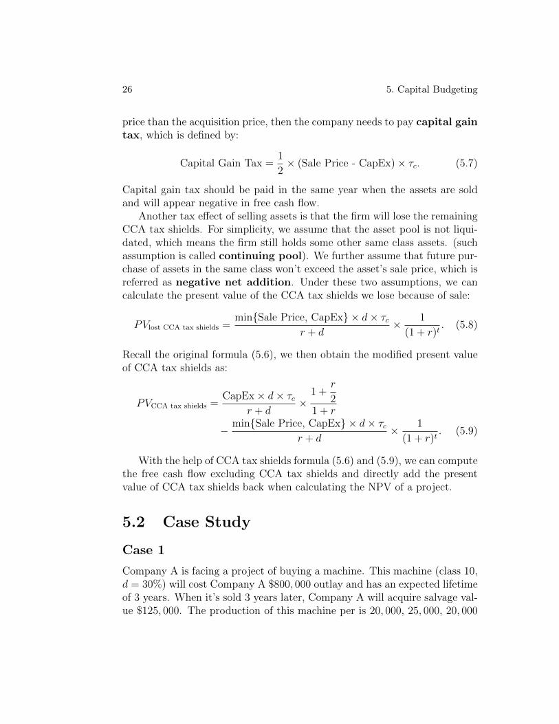
26 5. Capital Budgeting

price than the acquisition price, then the company needs to pay capital gaintax, which is defined by:

Capital Gain Tax =1

2× (Sale Price - CapEx)× τc. (5.7)

Capital gain tax should be paid in the same year when the assets are soldand will appear negative in free cash flow.

Another tax effect of selling assets is that the firm will lose the remainingCCA tax shields. For simplicity, we assume that the asset pool is not liqui-dated, which means the firm still holds some other same class assets. (suchassumption is called continuing pool). We further assume that future pur-chase of assets in the same class won’t exceed the asset’s sale price, which isreferred as negative net addition. Under these two assumptions, we cancalculate the present value of the CCA tax shields we lose because of sale:

PVlost CCA tax shields =minSale Price, CapEx × d× τc

r + d× 1

(1 + r)t. (5.8)

Recall the original formula (5.6), we then obtain the modified present valueof CCA tax shields as:

PVCCA tax shields =CapEx× d× τc

r + d×

1 +r

21 + r

− minSale Price, CapEx × d× τcr + d

× 1

(1 + r)t. (5.9)

With the help of CCA tax shields formula (5.6) and (5.9), we can computethe free cash flow excluding CCA tax shields and directly add the presentvalue of CCA tax shields back when calculating the NPV of a project.

5.2 Case Study

Case 1

Company A is facing a project of buying a machine. This machine (class 10,d = 30%) will cost Company A $800, 000 outlay and has an expected lifetimeof 3 years. When it’s sold 3 years later, Company A will acquire salvage val-ue $125, 000. The production of this machine per is 20, 000, 25, 000, 20, 000

5.2. Case Study 27

(units) in the coming 3 years and each unit is worth $100 and costs $80.Besides the costs of production, there is another fixed cost $50, 000 per yearto maintain the machine. The initial working capital is $30, 000 and needs10% of sales for maintenance. The corporate tax rate for Company A is 40%and the cost of capital is 10%.

Firstly, based on the production information and unit price, we can com-pute the sales in 3 years as:

S1 = S3 = 20, 000× 100 = $2, 000, 000, S3 = 25, 000× 100 = $2, 500, 000.

Similarly, the costs each year can be obtained by:

E1 = E3 = 20, 000× 80 + 50, 000 = $1, 650, 000,

E2 = 25, 000× 80 + 50, 000 = $2, 050, 000.

Then we can get the gross profits by:

(S1 − E1) = (S3 − E3) = $350, 000, (S2 − E2) = $450, 000.

Secondly, the NWC of the project is given as:

NWC0 = $30, 000, NWC1 = S1 × 10% = $200, 000,

NWC2 = S2 × 10% = $250, 000, NWC3 = S3 × 10% = $200, 000.

and so we can easily get the change of NWC

∆NWC0 = $30, 000, ∆NWC1 = $170, 000,

∆NWC2 = $50, 000, ∆NWC3 = −$250, 000.

Notice that we use ’same year’ rule when calculating NWC and ∆NWC.However, in textbook [1], they use the ’next year’ rule in order to keepconsistent with CCA tax shields’ calculation. Besides, we know CapEx0 =$800, 000 and CapEx3 = −$125, 000. Then we can calculate the free cashflows excluding CCA tax shields as:

CF0 = −CapEx0 −∆NWC0 = −800, 000− 30, 000 = −$830, 000,

CF1 = (S1 − E1)× (1− τc)−∆NWC1 = 350, 000× 60%− 170, 000 = $40, 000,

CF2 = (S2 − E2)× (1− τc)−∆NWC2 = 450, 000× 60%− 50, 000 = $222, 000,

CF3 = (S3 − E3)× (1− τc)− CapEx3 −∆NWC3

= 350, 000× 60% + 125, 000 + 250, 000 = $585, 000.

28 5. Capital Budgeting

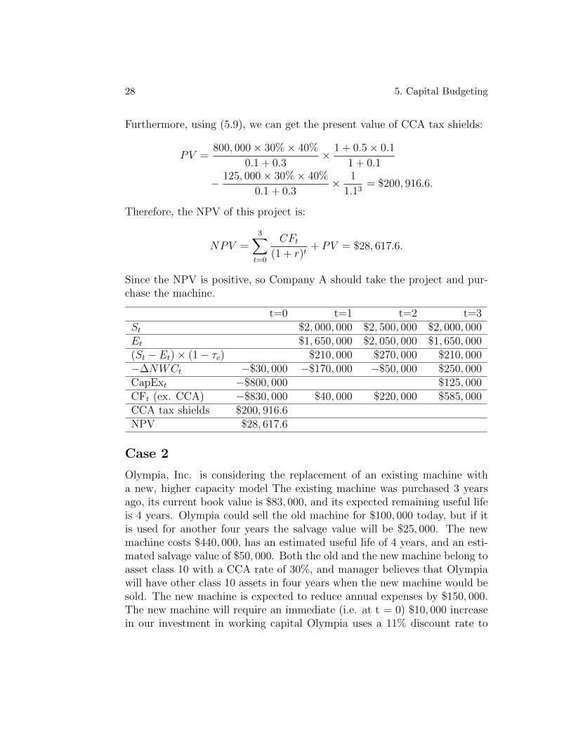
Furthermore, using (5.9), we can get the present value of CCA tax shields:

PV =800, 000× 30%× 40%

0.1 + 0.3× 1 + 0.5× 0.1

1 + 0.1

− 125, 000× 30%× 40%

0.1 + 0.3× 1

1.13= $200, 916.6.

Therefore, the NPV of this project is:

NPV =3∑

t=0

CFt

(1 + r)t+ PV = $28, 617.6.

Since the NPV is positive, so Company A should take the project and pur-chase the machine.

t=0 t=1 t=2 t=3St $2, 000, 000 $2, 500, 000 $2, 000, 000Et $1, 650, 000 $2, 050, 000 $1, 650, 000(St − Et)× (1− τc) $210, 000 $270, 000 $210, 000−∆NWCt −$30, 000 −$170, 000 −$50, 000 $250, 000CapExt −$800, 000 $125, 000CFt (ex. CCA) −$830, 000 $40, 000 $220, 000 $585, 000CCA tax shields $200, 916.6NPV $28, 617.6

Case 2

Olympia, Inc. is considering the replacement of an existing machine witha new, higher capacity model The existing machine was purchased 3 yearsago, its current book value is $83, 000, and its expected remaining useful lifeis 4 years. Olympia could sell the old machine for $100, 000 today, but if itis used for another four years the salvage value will be $25, 000. The newmachine costs $440, 000, has an estimated useful life of 4 years, and an esti-mated salvage value of $50, 000. Both the old and the new machine belong toasset class 10 with a CCA rate of 30%, and manager believes that Olympiawill have other class 10 assets in four years when the new machine would besold. The new machine is expected to reduce annual expenses by $150, 000.The new machine will require an immediate (i.e. at t = 0) $10, 000 increasein our investment in working capital Olympia uses a 11% discount rate to

5.2. Case Study 29

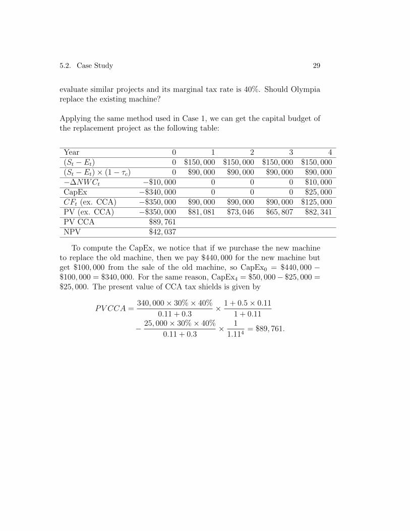
evaluate similar projects and its marginal tax rate is 40%. Should Olympiareplace the existing machine?

Applying the same method used in Case 1, we can get the capital budget ofthe replacement project as the following table:

Year 0 1 2 3 4(St − Et) 0 $150, 000 $150, 000 $150, 000 $150, 000(St − Et)× (1− τc) 0 $90, 000 $90, 000 $90, 000 $90, 000−∆NWCt −$10, 000 0 0 0 $10, 000CapEx −$340, 000 0 0 0 $25, 000CFt (ex. CCA) −$350, 000 $90, 000 $90, 000 $90, 000 $125, 000PV (ex. CCA) −$350, 000 $81, 081 $73, 046 $65, 807 $82, 341PV CCA $89, 761NPV $42, 037

To compute the CapEx, we notice that if we purchase the new machineto replace the old machine, then we pay $440, 000 for the new machine butget $100, 000 from the sale of the old machine, so CapEx0 = $440, 000 −$100, 000 = $340, 000. For the same reason, CapEx4 = $50, 000− $25, 000 =$25, 000. The present value of CCA tax shields is given by

PV CCA =340, 000× 30%× 40%

0.11 + 0.3× 1 + 0.5× 0.11

1 + 0.11

− 25, 000× 30%× 40%

0.11 + 0.3× 1

1.114= $89, 761.

Chapter 6

Bond and Stock Valuations

A Bond is a financial debt security, which stipulates the issuer of the bond(debtor) is obligated to pay the owners of the bond (creditor) certain interest(coupon) and/or repay the principal at maturity date. Generally, instrumentswith maturities less than one year are called Money Market Instrumentsinstead of bonds. A stock (also known as an equity or a share) is an instru-ment that signifies an ownership position (called equity) in a corporation,and represents a claim on its proportional share in the corporation’s assetsand profits.

Bonds and stocks are both securities, but a major difference is that (capi-tal) stockholders have an equity stake in the company (i.e., they are owners),whereas bondholders have a creditor stake in the company (i.e., they arelenders). Another difference is that bonds usually have a defined term, ormaturity, whereas stocks may be outstanding indefinitely. An exception is aconsol bond, which is a perpetuity (i.e., bond with no maturity). [11]

6.1 Valuing Bonds

The principal of a bond (face value) is the notational amount we use tocalculate the interest payments. For instance, if a bond contract has a couponrate rc (annual rate), face value C and the number of payments n per year,then its each coupon payment (CPN) is given by:

CPN =rc × Cn

. (6.1)

The simplest bond is zero-coupon bond. From its name, we know that

30

6.1. Valuing Bonds 31

such bond won’t pay interest but only repay the principal at maturity time.Examples are treasury bills. Since there is no coupon and money has timevalue, zero-coupon bond will always be sold at a price less than its face value,thus we can call it pure discount bond. A very important function of zero-coupon bond is to provide a good estimator of spot interest rate, but hereit has a special name, yield to maturity or simply yield. For example, anewly issued one-year government zero-coupon bond is sold at P0 = $952.38(face value is C = $1000.), then we can calculate the implied interest rate(investors’ expected interest rate):

r =C

P0

− 1 = 5%.

According to such argument, if we have infinitely many zero-coupon bondswith nearly continuous maturities (we can find zero-coupon bond with anymaturity), then we can obtain the approximately continuous interest rate,which is very useful in asset pricing. But in real life, we don’t have enoughzero-coupon bonds to plot a continuous line of interest rate versus time, sowe use numerical methods and finite (time, yield) data to construct yieldcurve. Probably, the most effective method is B splint interpolation while acommonly used one is simple polynomial interpolation. Besides, stochasticmodel (called term structure model) can also be used to capture thedynamics of yield. In contrary, the pricing of zero-coupon bond is simple,as long as we know the discount rate with the same maturity of bond, thenwe can simply discount back to get the price. Let C be the face value,remaining lifetime of bond is T (years) and interest rate of T years is rT orannual interest r, then the price is:

P =C

1 + rTor P =

C

(1 + r)T. (6.2)

Basically, all the other types of bond can be called coupon bond. Here,for simplicity, we only discuss fixed rate bonds. But in financial markets,there are indeed floating rate bonds (linked to the interest rate of some otherassets, like LIBOR, even inflation rate). Consider a coupon bond with facevalue C, coupon rate rc, number of payments n per period and maturity Nperiods. Assume yield rate per period is r, the cash flows of this bond canbe decomposed into an annuity plus a fixed inflow at maturity time. So the

32 6. Bond and Stock Valuations

present value (issue price) is given by:

P0 =CPN

r

(1− 1

(1 + r)N

)+

C

(1 + r)N, (6.3)

where CPN can be calculated through (6.1).Example. We have the following there bonds:

Bond C rc T n rBond 1 $1, 000 10% 4 2 4%Bond 2 $1, 000 10% 4 2 5%Bond 3 $1, 000 10% 4 2 6%

Solution. Using (6.1) to calculate CPN, for bond 1, we have CPN1 =1000×10%

2= $50. Notice r is the yield per period, (half year in this example),

so we can directly use (6.3) to obtain the price of bond 1 as: (N = T×n = 8)

P 10 =

50

0.04

(1− 1

1.048

)+

1000

1.048= $1067.33 > C.

By the same method, we can also calculate the prices of bond 2 and 3 by:

P 20 =

50

0.05

(1− 1

1.058

)+

1000

1.058= $1000 = C,

P 30 =

50

0.06

(1− 1

1.068

)+

1000

1.068= $937.90 < C.

From the above example, we can summarize that

r <rcn⇔ P0 > C (premium)

r =rcn⇔ P0 = C (par)

r >rcn⇔ P0 < C (discount)

The rigorous proof is easy. Denote rcn·r by a, then we can rewrite (6.3) as

P0 = aC

(1− 1

(1 + r)N

)+

C

(1 + r)N

= C + (a− 1)C

(1− 1

(1 + r)N

)⇒ P0 − C = (a− 1)C

(1− 1

(1 + r)N

)⇒ Sign(P0 − C) = Sign(a− 1),

6.1. Valuing Bonds 33

which Sign(x) is the sign of x. Since yield is not constant through the whole maturity period of a bond,

bond value will change as yield changes. An obvious relation is that whenyield rate goes up, bond value will decrease and vise versa. However, we stillwant to find a measurement for bond’s sensitivity to the change of interestrate. An intuitive idea is use maturity, but the following example will showthat maturity is an imperfect measure of sensitivity against interest rate.

Example. Consider two bonds and list the information as follows:

Bond C rc T n r1 r2

Bond A $1, 000 10% 10 1 10% 4%Bond B $1, 000 4% 9 1 10% 4%

Case 1. r = r1 = 10%Since r = rAc , PA

0 = $1, 000. For bond B, its price is given by:

PB0 =

40

0.1

(1− 1

(1 + 0.1)9

)+

1000

(1 + 0.1)9= $654.46

Case 2. r = r2 = 4%In this case, r = rBc , so PB

0 = $1, 000. For bond A, we can calculate its priceby:

PA0 =

100

0.1

(1− 1

(1 + 0.04)10

)+

1000

(1 + 0.04)10= $1, 486.65

Therefore, we can obtain the percent of change of prices for two bonds:

%∆A =1486.65

1000− 1 = 48.7%

%∆B =1000

654.46− 1 = 52.8%

This example shows that the bond with shorter maturity time can bemore sensitive to the change of interest rate. So we have the accurate measureduration, which is defined by:

D =1

P0

T∑t=1

CFt

(1 + r)t× t, (6.4)

where CFt = CPN, 1 ≤ t ≤ T − 1 and CFT = CPN + C.

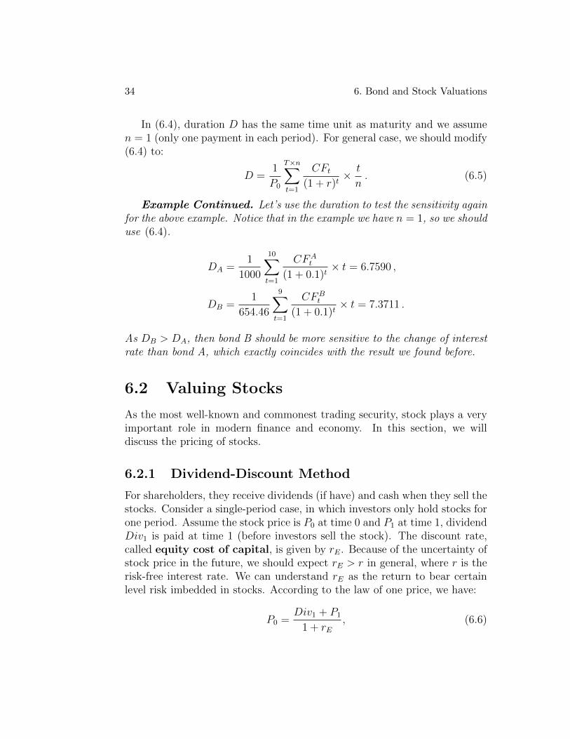
34 6. Bond and Stock Valuations

In (6.4), duration D has the same time unit as maturity and we assumen = 1 (only one payment in each period). For general case, we should modify(6.4) to:

D =1

P0

T×n∑t=1

CFt

(1 + r)t× t

n. (6.5)

Example Continued. Let’s use the duration to test the sensitivity againfor the above example. Notice that in the example we have n = 1, so we shoulduse (6.4).

DA =1

1000

10∑t=1

CFAt

(1 + 0.1)t× t = 6.7590 ,

DB =1

654.46

9∑t=1

CFBt

(1 + 0.1)t× t = 7.3711 .

As DB > DA, then bond B should be more sensitive to the change of interestrate than bond A, which exactly coincides with the result we found before.

6.2 Valuing Stocks

As the most well-known and commonest trading security, stock plays a veryimportant role in modern finance and economy. In this section, we willdiscuss the pricing of stocks.

6.2.1 Dividend-Discount Method

For shareholders, they receive dividends (if have) and cash when they sell thestocks. Consider a single-period case, in which investors only hold stocks forone period. Assume the stock price is P0 at time 0 and P1 at time 1, dividendDiv1 is paid at time 1 (before investors sell the stock). The discount rate,called equity cost of capital, is given by rE. Because of the uncertainty ofstock price in the future, we should expect rE > r in general, where r is therisk-free interest rate. We can understand rE as the return to bear certainlevel risk imbedded in stocks. According to the law of one price, we have:

P0 =Div1 + P1

1 + rE, (6.6)

6.2. Valuing Stocks 35

which can be rewritten as

rE =Div1 + P1

P0

− 1 =Div1

P0

+P1 − P0

P0

, (6.7)

where the first fraction is called stock’s dividend yield while the secondone is capital gain rate.

Then we extend our discussion to multi-period models. If investors holdstock from time 1 to time 2, then they will get dividend Div2 paid at time2 and cash P2 when they sell the stock after collecting the dividend. So wehave:

P1 =Div2 + P2

1 + rE, (6.8)

which gives us

P0 =

[Div2 + P2

1 + rE+Div1

]1

1 + rE

=Div1

1 + rE+

Div2

(1 + rE)2+

P2

(1 + rE)2. (6.9)

If investors hold the stock forever, then they can get all the dividends Divt atpayment date t (similar to perpetuity with cash flows Divt). So again usingthe law of one price, we can expect to obtain:

P0 =∞∑t=1

Divt(1 + rE)t

. (6.10)

If dividend grows at a constant rate g, then by (3.13), we can get the priceof stock by:

P0 =Div1

rE − g, g < rE. (6.11)

Example of Changing Growth Rate. Assume the stock of NielsenMotors has expected dividend $5 per share next year and its expected growthrate will be 8% until year 8 and change to 3$ after year 8. The discount rate(cost of capital) is rE = 12%.

Solution. We can decompose all the cash flows of the stock into a growingannuity and a growing perpetuity. For this annuity, we know its first paymentDiv1 = $5, growth rate g1 = 8% and the total number of payments N = 8,so we can calculate the present value of this growing annuity:

PVA =Div1

rE − g1

[1− (1 + g1)N

(1 + rE)N

]=

5

0.12− 0.08

[1− (1.08)8

(1.12)8

]= $31.55.

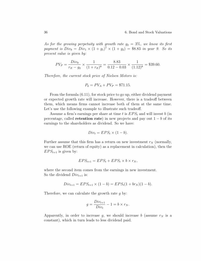
36 6. Bond and Stock Valuations

As for the growing perpetuity with growth rate g2 = 3%, we know its firstpayment is Div9 = Div1 × (1 + g1)7 × (1 + g2) = $8.83 in year 9. So itspresent value is given by:

PVP =Div9

rE − g2

× 1

(1 + rE)8=

8.83

0.12− 0.03× 1

(1.12)8= $39.60.

Therefore, the current stock price of Nielsen Motors is:

P0 = PVA + PVP = $71.15.

From the formula (6.11), for stock price to go up, either dividend paymentor expected growth rate will increase. However, there is a tradeoff betweenthem, which means firms cannot increase both of them at the same time.Let’s use the following example to illustrate such tradeoff.

Assume a firm’s earnings per share at time t is EPSt and will invest b (inpercentage, called retention rate) in new projects and pay out 1− b of itsearnings to the shareholders as dividend. So we have:

Divt = EPSt × (1− b).

Further assume that this firm has a return on new investment rN (normally,we can use ROE (return of equity) as a replacement in calculation), then theEPSt+1 is given by:

EPSt+1 = EPSt + EPSt × b× rN ,

where the second item comes from the earnings in new investment.So the dividend Divt+1 is:

Divt+1 = EPSt+1 × (1− b) = EPSt(1 + brN)(1− b).

Therefore, we can calculate the growth rate g by:

g =Divt+1

Divt− 1 = b× rN .

Apparently, in order to increase g, we should increase b (assume rN is aconstant), which in turn leads to less dividend paid.

6.2. Valuing Stocks 37

6.2.2 Comparison Method

In this section, we can use the ratios discussed in chapter 2 to estimate thestock price. A possible candidate is P/E ratio. We will demonstrate how toapply comparison method to estimate the stock price using P/E ratio by thefollowing example.

Example. Bergeron’s earnings per share is EPS1 = $2 and dividend pershare is Div1 = $1.2 and has a cost of capital rE = 14% and ROE 16%.Then we can its growth rate g by:

g = (1− Div1

EPS1

)×ROE = 40%× 16% = 6.4%.

So Bergeron’s stock price can be obtained through:

P0 =Div1

rE − g=

1.2

0.14− 0.064= $15.79.

Accordingly, we can calculate its P/E ratio by:

P/E =P0

EPS1

=15.79

2= 7.89.

Assume there is another company whose stocks are not publicly traded andthis company is similar to Bergeron’s (assumption implies that they share thesame or similar P/E ratio). Besides, they also have the same cost of capitaland growth rate. The earnings per share of the company next year is expectedto be EPS ′1 = $5. Then applying the comparison method, we have:

P ′0 = P/E × EPS ′1 = 7.89× 5 = $39.47.

Remark. In the previous example, we use so-called forward earnings(expected earnings in the coming year) when calculating P/E ratio. Corre-spondingly, we can also use trailing earnings (earnings in the last year) tocompute P/E ratio.

Except P/E ratio, we can also use enterprise value multiples. Recall thedefinition of enterprise value:

Enterprise Value = Market Value of Equity + Cash - Debt.

38 6. Bond and Stock Valuations

We can use free cash flow formula (5.5) to estimate enterprise value. Let V0

be the present value of all free cash flows, then the current enterprice valuecan be obtained by:

Enterprise Value = V0 + PV(Cash)-PV(Debt). (6.12)

Then we can estimate the share price by the following formula:

P0 =V0 + PV(Cash)-PV(Debt)

Number of Outstanding Shares(6.13)

In order to computer V0, we need to discount all the free cash flows andwe cannot use the discount rate rE because the free cash flows will be paid toboth equity holders and debt holders. Instead, we should use the weightedaverage cost of capital (WACC), rWACC , as the discount rate:

rWACC =E

V× rE +

D

V× rD, (6.14)

where E, D V are equity value, debt value and firm value while rD is thecost of debt. If the free cash flows have a constant growth rate gFCF , thenwe can obtain the formula for Vt (present value in year t):

Vt =CFt+1

rWACC − gFCF

. (6.15)

Dividing by EBIT (earnings before interest and taxes) or EBITDA (earningsbefore interest, taxed, depreciation, and amortization), we will get a goodmultiple:

V0

EBIT1

=CF1/EBIT1

rWACC − gFCF

. (6.16)

Chapter 7

Options

7.1 Introduction

In finance, an option is a derivative instrument which offers the holder theright but not the obligation to sell (put option) or buy (call option) cer-tain asset(s) at pre-specified price (called strike price or exercise price)during a specified time frame. For a European option, the holders canonly exercise the option at maturity; but an American option allows itsholders to exercise their right at any time prior to expiration.

Consider a European call option with underlying asset (price St at timet), strike price K and maturity time T , then the payoff at time T is:

CT = (ST −K)+, (7.1)

and the profit at time T is: (ignore the time value of money or assume r = 0)

VT = (ST −K)+ − C0, (7.2)

where C0 is the call option price at time 0.Similarly, for a European put option with all same settings, we have its

payoff function at time T :

PT = (K − ST )+, (7.3)

and the profit at time T is:

VT = (K − ST )+ − P0, (7.4)

39

40 7. Options

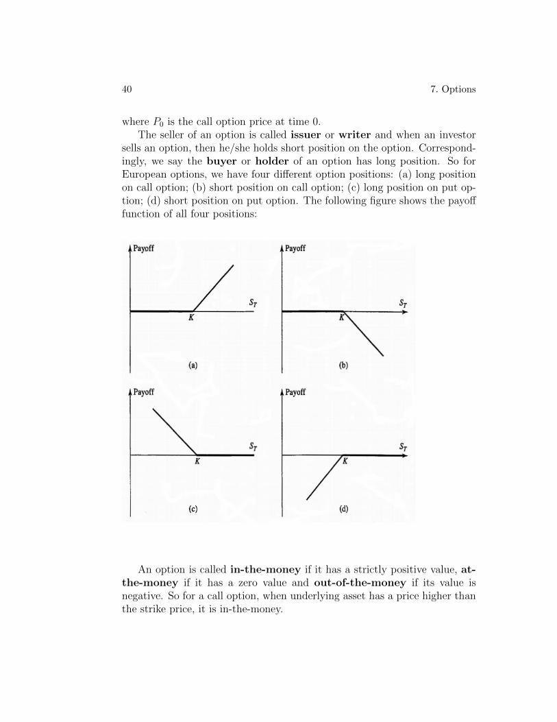
where P0 is the call option price at time 0.The seller of an option is called issuer or writer and when an investor

sells an option, then he/she holds short position on the option. Correspond-ingly, we say the buyer or holder of an option has long position. So forEuropean options, we have four different option positions: (a) long positionon call option; (b) short position on call option; (c) long position on put op-tion; (d) short position on put option. The following figure shows the payofffunction of all four positions:

An option is called in-the-money if it has a strictly positive value, at-the-money if it has a zero value and out-of-the-money if its value isnegative. So for a call option, when underlying asset has a price higher thanthe strike price, it is in-the-money.

7.2. Properties of Stock Options 41

7.2 Properties of Stock Options

The commonest option is stock option. However, there are many optionswhich have underlying assets like futures, exchange, index and even otheroptions. In what follows, we will focus on stock options and discuss theirproperties.

7.2.1 Factors Affecting Option Prices

Firstly, we want to study how different factors affect option prices. Thefactors in consideration are current stock price S0, strike price K, maturitytime T , volatility of stock σ, risk-free interest rate r and dividends withinexpiration period. When we discuss the impact of one factor, we assume allthe other factors remain same.

Stock Price. For a call option, the higher the stock price, the morelikely it will end up with a positive value and the more profit the holders canpossibly get. For this reason, the price of a call option should move in thesame direction as the underlying stock price. However, for a put option, weencounter the exactly opposite case.

Strike Price. From the payoff functions, we know that strike priceplays the contrary role in payoff comparing to stock price, which means theincrease of stock price has the same impact as the decrease of strike price.In consequence, strike price is negatively correlated with the price of calloptions but positively correlated with the price of put options.

Maturity Time. For American options, the impact of maturity time onoption prices is obvious. Since the buyers of American options can exerciseoptions at any time up to maturity time, the longer the maturity the morebenefit buyers may get. Therefore, both American call and put options willincrease in value when maturity gets longer. Usually, same results also applyto European options. However, we cannot claim such relationship for sure.For instance, if there is a up-coming huge dividend in 3 months (dividendwill cause the drop of stock price), then a call option which will expire within3 months is more valuable than those with maturity longer than 3 months.

Volatility. Notice that the payoff of options is always non-negative, andthe more volatile the stock price is, the more likely that the stock price willexceed the threshold value (strike price). For instance, consider two cases:(Case 1) stock price S0 = $50 will go to either $80 or $20; (Case 2) stockprice S0 = $50 will go to either $100 or $0. Apparently, the stock in case 2

42 7. Options

is more volatile and for a call option with strike price K = $50, the payoffin case 1 is either $30 or 0 while in case 2 the payoff will be either $50 or 0.Therefore, options on the second stock are dominant at both scenarios andthus should have higher prices than options on the first stock.

Risk-free Interest Rate. The relationship between the risk-free interestrate r and option prices is hard to discuss using general analysis. On oneside, if r goes up, the expected return of stock should increase as well; buton the other hand, the increase of r will make the future payoff of optionsless valuable. The result is that call options have a positive correlation withthe risk-free interest rate but put options have a negative correlation withthe risk-free interest rate. We will come back to this issue later in continuousmodel.

Dividend. It’s clear that the payment of dividends will reduce the stockprice on the ex-dividend date and so we should anticipate that the factor ofdividend has the opposite impact as stock price does.

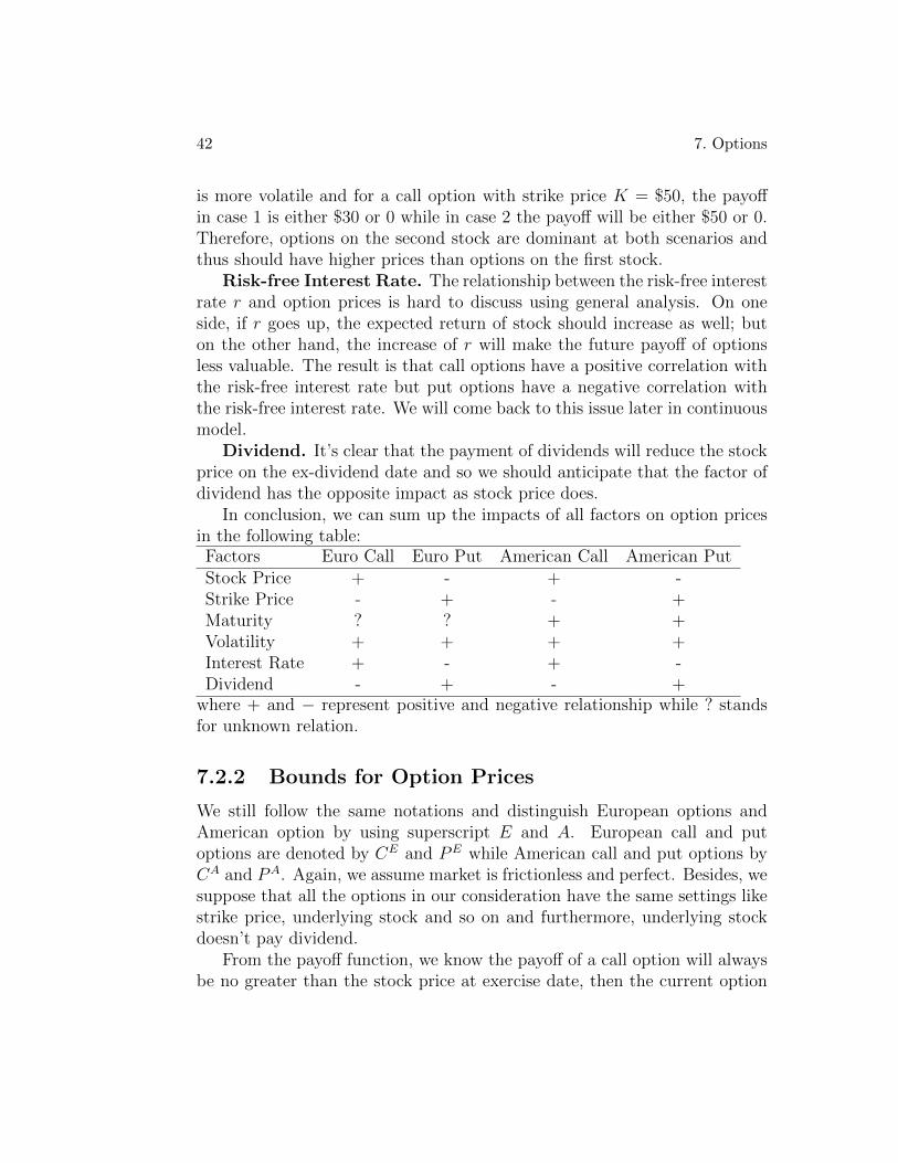
In conclusion, we can sum up the impacts of all factors on option pricesin the following table:Factors Euro Call Euro Put American Call American PutStock Price + - + -Strike Price - + - +Maturity ? ? + +Volatility + + + +Interest Rate + - + -Dividend - + - +

where + and − represent positive and negative relationship while ? standsfor unknown relation.

7.2.2 Bounds for Option Prices

We still follow the same notations and distinguish European options andAmerican option by using superscript E and A. European call and putoptions are denoted by CE and PE while American call and put options byCA and PA. Again, we assume market is frictionless and perfect. Besides, wesuppose that all the options in our consideration have the same settings likestrike price, underlying stock and so on and furthermore, underlying stockdoesn’t pay dividend.

From the payoff function, we know the payoff of a call option will alwaysbe no greater than the stock price at exercise date, then the current option

7.2. Properties of Stock Options 43

price should be no greater than the current stock price. Such argument leadsto the upper bounds of call option:

CE ≤ S0, and CA ≤ S0. (7.5)

Similarly, the maximum payoff a put option can get is equal to the strikeprice K, so the upper bounds of put options are:

PE ≤ K, and PA ≤ K. (7.6)

Since a European put option can only be exercised at maturity time T , sowe can further derive that

PE ≤ Ke−rT . (7.7)

To get the lower bound of a European call option, consider two portfolios:the first one consists of one share European call option and Ke−rT cash inrisk-free account while the second is just one share of stock. At time 0,the first portfolio has value V 1

0 = CE +Ke−rT and the second one has valueV 2

0 = S0. At time T , we have V 1T = (ST−K)++K and V 2

T = ST . Apparently,V 1T ≥ V 2

T , then by the law of one price, we should have V 10 ≥ V 2

0 . A littlearrangement plus the non-negative property of option price give us:

max(S0 −Ke−rT , 0) = (S0 −Ke−rT )+ ≤ CE. (7.8)

By the same token, just consider a portfolio of one European put optionand one share of stock while another portfolio of Ke−rT cash in risk-freeacount, we can get the lower bound of European put option:

max(Ke−rT − S0, 0) = (Ke−rT − S0)+ ≤ PE. (7.9)

Since we assume there is no dividend payment, an American call optionshould have the exactly same price as the corresponding European call option.The reason is simple, firstly, notice that CA ≥ CE and (S0−Ke−rT )+ ≤ CE.However, if we exercise a in-the-money American call right now, we can onlyget S0 −K < S0 −Ke−rT .

The formal proof can be made as follows: assume CA > CE and considera portfolio which consists of buying one share European call option, sellingone share American option and investing CA − CE cash in bank account atrate r.

At time 0

44 7. Options

It’s obvious that our portfolio has a zero value.At early exercise time t ≤ TWe need to borrow one share of stock and sell it at price K to the buyer

of the American call option, and then invest K in bank account again at rater.

At maturity time TSince American call has already been exercised, it contributes nothing at

T . As we borrowed one share stock at time t, we can exercise our Europeancall at time T to buy one share at price K and clear our position on stock.From bank account, we can get (CA − CE)erT + Ker(T−t). Therefore, thevalue at final time is:

VT = (CA − CE)erT +Ker(T−t) −K > 0.

We just constructed an arbitrage portfolio, which is a contradiction to thelaw of one price. Therefore, we have:

CA = CE ≥ (S0 −Ke−rT )+.

However, for an American put option, early exercise may be favorable.Just consider an extreme example, assume the current stock price is 0 ornearly 0, then exercising now will give us the profit K, which is the maximumprofit we can possibly obtain. Besides, we can invest K in bank account andgain extra interest. So under this extreme case, we should exercise early.Since for any in-the-money American put option, the least we can get rightnow is K − S0 by early exercise. Therefore, we shall have

(K − S0)+ ≤ PA. (7.10)

In summarization, we have the following bounds for option prices:

(S0 −Ke−rT )+ ≤ CA = CE ≤ S0, (7.11)

(Ke−rT − S0)+ ≤ PE ≤ Ke−rT , (7.12)

and (K − S0)+ ≤ PA ≤ K. (7.13)

Remark. [5] If the underlying stock pays dividends during the expirationperiod of options, then the lower bounds need to be modified. Basically, wecan understand the payment of dividends has the similar impact on optionprices as the decrease of stock price does. So use D to denote the present

7.2. Properties of Stock Options 45

value of all dividend payments during expiration period, then by the sameno-arbitrage argument (omit the detailed proof here), we have:

S0 −D −KerT ≤ CE, (7.14)

D +KerT − S0 ≤ PE. (7.15)

Besides, we can also conclude that it’s only possible to exercise an Americancall option immediately prior to an ex-dividend date.

7.2.3 Put-Call Parity

Put-call parity is an important relationship between European call and putoptions. To derive such parity, we construct the following portfolio:

• buy one share call option

• sell one share put option

• sell one share underlying stock

• lend Ke−rT money at rate r

At time 0, the value of this portfolio is:

V0 = −CE + PE + S0 −Ke−rT ,

where + means cash inflow while − means cash outflow.At time T , the value of the portfolio is:

VT = (ST −K)+ − (K − ST )+ − ST +K

=

ST −K + 0− ST +K = 0 ; ST > K0−K + ST − ST +K = 0 ; ST ≤ K

= 0

So by no-arbitrage theory, we should expect V0 = 0 and have the followingput-call parity:

CE +Ke−rT = PE + S0. (7.16)

However, for American call and put options, we don’t have the put-callparity. If we further assume there is no dividend payment for the underlyingstock, then instead we will have the following inequality:

S0 −K ≤ CA − PA ≤ S0 −Ke−rT . (7.17)

To show the left side, consider the following two portfolios:

46 7. Options

• a) One share American call option and K cash in bank account

• b) One share American put option and one share stock

At time 0, we have:

V a0 = CA +K, and V b

0 = PA + S0.

Notice that it is always not optimal to exercise an American call option,but it might be optimal to exercise an American put option before the ma-turity time. Let us assume investors will exercise this American put at timet ≤ T . At time t, for Portfolio b, investors will sell the stock they purchasedat time 0 at price K and then reinvest K into a bank account at rate r.At maturity time T , the value of Portfolio a is:

V aT = (ST −K)+ +KerT =

ST +K(erT − 1) : ST ≥ KKerT : ST < K

If there is no early exercise, the value of Portfolio b is:

V bT = (K − ST )+ + ST =

ST : ST ≥ KK : ST < K

If investors exercise the put option at an early time, and reinvest K in abank account, then the value of Portfolio b is:

V bT = Ker(T−t).

But no matter in which case, we always have:

V aT ≥ V b

T .

Therefore, by the law of one price, we must have:

V a0 ≥ V b

0 ,

which gives us thatS0 −K ≤ CA − PA.

For the other side, consider two portfolios:

• a) One share American call option and Ke−rT cash in bank account

7.3. The Binomial Pricing Model 47

• b) One share American put option and one share stock

At time 0, we have:

V a0 = CA +Ke−rT , and V b

0 = PA + S0.

At maturity time T , the value of portfolio a is:

V aT = (ST −K)+ +K =

ST : ST ≥ KK : ST < K

For investors of Portfolio b, they can always wait until the maturity timeto make decision, either exercise the put to sell the stock at K (K > ST ) orsell the stock at market price to get ST (ST ≥ K). Either way, the value ofPortfolio b at time T is always no less than V a

T :

V bT ≥ V a

T ,

which directly impliesV b

0 ≥ V a0 ,

or equivalentlyCA − PA ≤ S0 −Ke−rT .

Another alternative proof of the right side inequality is to notice theput-call parity and CE = CA , PE ≤ PA, and hence

CA − PA ≤ CE − PE = S0 −Ke−rT .

Remark.[5] If we take dividends into consideration, the put-call paritywill be:

CE +Ke−rT = PE + S0 −D, (7.18)

while (7.17) should be changed to:

S0 −D −K ≤ CA − PA ≤ S0 −Ke−rT . (7.19)

7.3 The Binomial Pricing Model

Firstly, let us consider a single-period binomial model. Assume the currentunderlying stock price is S0 and will either go up to S1(U) = uS0 withprobability p > 0 or go down to S1(D) = dS0 with probability q = 1− p > 0.Moreover, we assume u > d.

48 7. Options

S0

>

S1(U) = uS0

ZZZZZZZZZ~ S1(D) = dS0

The risk-free interest rate (nominal rate) is r, which means holding onedollar today will give you (1 + r) dollars in period 1. In order to guaranteethe positiveness, we assume r > −1 and in real life r is always non-negative.

Proposition 1. In this single-period binomial model, the following con-dition has to be satisfied in order to guarantee no-arbitrage:

0 < d < 1 + r < u. (7.20)

The proof to this proposition is easy and we just show the left inequality.Assume to the contrary that:

d ≥ 1 + r,

which means even in the worst scenario, stock still dominates the bank ac-count. So we should lend S0 at rate r and use the money to buy one sharestock from market. Apparently, our portfolio has zero value at time 0. Attime 1, our portfolio will worth either uS0−(1+r)S0 > 0 or dS0−(1+r)S0 ≥ 0.Then we have constructed an arbitrage portfolio, which suggests

d < 1 + r.

We introduce an European call option, which has strike price K and willexpire at time 1. Furthermore, we assume S1(D) < K < S1(U), otherwisethe pricing becomes trivial. Therefore, for this call option, we can write itsvalue at time 1 as

C1(U) = (S1(U)−K)+ = S1(U)−K, and C1(D) = (S1(D)−K)+ = 0.

7.3. The Binomial Pricing Model 49

In order to price this European call option, we try to find a replicationportfolio (the one with the same cash flows) using only stock and risk-free as-set (bank account). Assume we can find a replication portfolio which worthsV0 and composes of buying ∆ shares of stock and investing V0−∆S0 in bankaccount. Then at time 1, the value of this portfolio is given by:

V1 =

∆S1(U) + (1 + r)(V0 −∆S0)∆S1(D) + (1 + r)(V0 −∆S0)

Since this is a replication portfolio (V1 = C1), then we must have:

∆S1(U) + (1 + r)(V0 −∆S0) = C1(U), (7.21)

∆S1(D) + (1 + r)(V0 −∆S0) = C1(D). (7.22)

Solving the above equations gives us that:

∆ =C1(U)− C1(D)

S1(U)− S1(D), (7.23)

and

V0 =1

1 + r[p∗ × C1(U) + q∗ × C1(D)] , (7.24)

where

p∗ =(1 + r)S0 − S1(D)

S1(U)− S1(D)and q∗ =

S1(U)− (1 + r)S0

S1(U)− S1(D). (7.25)

Since the solutions to the system of equations exist, we can actually findsuch replication portfolio which has exactly the same payoff at time 1 as theEuropean call option. Therefore, by the law of one price, we obtain the priceof the European option:

C0 =1

1 + r[p∗ × C1(U) + q∗ × C1(D)] . (7.26)

Because of the no-arbitrage condition (7.20), we can easily check that Q =(p∗, q∗) is a probability measure which is different from the actual probabilityP = (p, q). An interesting result is that the European call option has returnr under the measure Q. Simple calculation also shows that same resultapplies to the risk-free asset and stock. The measure Q is called risk-neutralprobability measure and all discounted securities under this measure are

50 7. Options

martingales and have the same return r regardless of investors’ risk preference(More rigorous definition will be given in the next section). Therefore, as longas we can find such measure, pricing securities becomes taking expectationunder Q. In our single-period model, Q is given by: di

p∗ =1 + r − du− d

andu− 1− ru− d

. (7.27)

Using this powerful tool, we can easily find the price of a European putoption with strike price K:

P0 =1

1 + r[p∗ × P1(U) + q∗ × P1(D)] . (7.28)

Example. The current stock price is S0 = 100 and its price at time1 will be either 150 or 100. An European call option written on this stockwith strike price 120 will expire at time 1. The risk-free interest rate is 10%.What the present value of this call option? What is the price of the sameEuropean put option?

Solution. Given the stock prices, we know u = 1.5, d = 1 and then cancalculate the risk-neutral probability measure Q = (0.2, 0.8). Therefore, theprice of call option is given by:

C0 =1

1.1[0.2× 30 + 0.8× 0] = 5.45,

while the put option price is:

P0 =1

1.1[0.2× 0 + 0.8× 20] = 14.55.

Besides, we can check the put-call parity by: (notice the corresponding changefrom Ke−r (continuous discount) to K

1+r(discrete discount))

S0 −K

1 + r= −9.1 = C0 − P0 ⇒ C0 +

K

1 + r= P0 + S0.

By the same idea, we can extend a single-period binomial model to amulti-period binomial model. The first step is to choose the total number ofperiods N and determine the value of European options at maturity time (inperiod N), and then using the formula (7.26) or (7.28) to go backwards tocalculate the expected value in period N − 1. Obviously, such procedure will

7.3. The Binomial Pricing Model 51

finally lead to C0 or P0. In order to make the binomial trees more compact,we assume ui = u and di = d, 1 ≤ i ≤ N and d = 1

u, then all the two

adjacent subtrees will share the same node. For instance, at time 2, we haveS2(UD) = S2(DU), where UD means stock price goes up in period 1 andgoes down in period 2.

Let’s take N = 3 as an example to show how to conduct backward pro-cedure. Firstly, under our assumption, we have:

S3(UUU) = u3S0, S3(UUD) = S3(UDU) = S3(DUU) = u2dS0,

S3(DDD) = d3S0, S3(DDU) = S3(DUD) = S3(UDD) = ud2S0.

Then for an European call option with strike price K, its payoff at maturitytime is:

C3 = (S3 −K)+.

To calculate the value of this call option in period 2 at state UU , we use:

S2(UU) =1

1 + r[p∗S3(UUU) + q∗S3(UUD)].

Similarly, we can also get:

S2(UD) = S2(DU) =1

1 + r[p∗S3(UUD) + q∗S3(UDD)],

and S2(DD) =1

1 + r[p∗S3(UDD) + q∗S3(DDD)].

Then in period 1,

S1(U) =1

1 + r[p∗S2(UU)+q∗S2(UD)], S1(D) =

1

1 + r[p∗S2(UD)+q∗S2(DD)].

Finally, we can obtain the price of this call option by:

C0 =1

1 + r[p∗S1(U) + q∗S1(D).]

The above method is the general way to do the backward estimation ofoption values. However, we can also directly find Q as

Q = ((p∗)3, 3(p∗)2(q∗), 3(p∗)(q∗)2, (q∗)3).

Then the option price can be given by:

C0 =1

(1 + r)3

[(p∗)3 · (u3S0 −K)+ + 3(p∗)2(q∗) · (u2dS0 −K)+

+ 3(p∗)(q∗)2 · (ud2S0 −K)+ + (q∗)3 · (d3S0 −K)+].

52 7. Options

7.4 Black-Scholes Model

In the previous section, we discussed how to price European options in dis-crete binomial model. Here we will continue our discussion on option pricingin continuous time. More specifically, we consider the well-known Black-Scholes (BS) model [2] for option pricing.

In continuous time, stock price is a stochastic process in mathematicalview, denoted by St. The key assumption in BS model is to set the dynamicsof stock price as:

dSt

St

= µdt+ σdWt, (7.29)

where µ ∈ R, σ > 0 are constants and Wt is a Brownian motion defined in astandard stochastic basis (Ω,F , (F)t≥0,P) 1.

By applying Ito’s formula to log(St), we get:

d(log(St)) =

(µ− σ2

2

)dt+ σdWt. (7.30)

We can write the above stochastic differential equation (SDE) in differenceform:

log

(St+∆t

St

)=

(µ− σ2

2

)∆t+σ∆Wt ∼ N

((µ− σ2

2

)∆t, σ2∆t

), (7.31)

where N stands for the standard normal distribution.In real industry, even the stock price changes continuously, the quoted

prices are still discrete, so how to estimate the parameters µ and σ usingdiscrete data is an important issue, while (7.31) gives us an appropriate wayto address this question. Firstly, from the discrete data of stock prices, wecan simply compute log return log(St+1/St), then with the help of statisticssoftwares like SAS, Eviews and SPSS, we can obtain the mean µ and varianceσ2. According to (7.31), we have:

µ = (µ− σ2

2)∆t, (7.32)

σ2 = σ2∆t. (7.33)

By solving the above equations, we can get the estimations of parameters.

1For further reading in stochastic calculus, please refer to [10].

7.4. Black-Scholes Model 53

Next, we need to give a formal definition of risk-neutral probability mea-sure Q: Q is an equivalent measure to P such that under this measure, theprice processes of all discounted securities are martingales. So our goal is tofind a Q such that the dt term in (7.29) is r instead of µ. Mathematically,

∀A ∈ F ,P(A) = 0⇔ Q(A) = 0 (equivalence) (7.34)

and

E∗[St|Fs] = Ss, t ≥ s (martingale property) (7.35)

where E∗ denotes the expectation under measure Q and S is the discountedprice of any underlying asset in the market. So if there are N risky assets,we should expect to have N martingale equations.

To this purpose, we make the following change of measure:

dQt

dPt

= ε

(−∫ t

0

λsdWs

)= exp

(−∫ t

0

λsdWs −1

2

∫ t

0

λ2sds

), (7.36)

where

λs = λ =µ− rσ

. (7.37)

Due to the strict positiveness of exponential function, P and Q are equivalent.Furthermore, define the following process by:

W ∗t = Wt +

∫ t

0

λds. (7.38)

The technical name of this transform is called change of Wiener process(another name of Brownian motion). According to Girsanov’s Theorem, W ∗

t

is a standard Brownian motion under measure Q. Under Q, we can see that

dSt

St

= µdt+ σ(dW ∗t − λdt) = rdt+ σdW ∗

t . (7.39)

In our setting, the underlying assets are risk-free asset and stock, so thenew measure Q defined by (7.36) is indeed a risk-neutral probability measure(actually, also the only one, since our market is complete).

Consider an European call option with strike price K and maturity T .Risk-free interest rate is given by r. Again, we assume our market is perfectand efficient. Besides, we need to put an additional assumption: the option

54 7. Options

price is a function of time t and stock price St, or mathematically, Ct =f(t, St).

Using Ito’s formula to f(t, St), we shall have:

df(t, St) = ftdt+ fsdSt +1

2fssdS

2t

= (ft + fsµSt +1

2fssσ

2S2t )dt+ fsσStdWt, (7.40)

where

ft =∂f

∂t, fs =

∂f

∂St

, fss =∂2f

∂S2t

.

Similar to the replication method used in binomial model, we constructa dynamic portfolio at time t by buying one share call option and selling fsshares stock, then the dynamics of our portfolio at time t is:

df(t, St)− fsdSt = (ft +1

2fssσ

2S2t )dt,

which is non-stochastic and so should have the return r for sure (otherwisewe can find arbitrage opportunity). This argument then gives:

(ft +1

2fssσ

2S2t )dt = r(f(t, St)− fsSt)dt.

Little arrangement gives us the famous SDE:

ft + rStfs +1

2σ2S2

t fss = rf(t, St). (7.41)

In addition, f should also satisfy the boundary condition at T

f(T, x) = (x−K)+. (7.42)

The solution to the above SDE with the boundary condition is solved in[2].

Chapter 8

Risk and Return

8.1 Statistics Background

Standard Deviation, the square root of variance, is also called volatilityin finance, which measures how much the observations (variables) differ fromits expectation (mean value) [12].

σ =√E[X − E(X)]2, (8.1)

where E(X) is the expected value of X.Notice that standard deviation and sample standard deviation have

slight difference. In calculating the former one, data should represent thewhole population. However, if we only have the data collected from a largerandom sample, then we can only compute the latter one. To estimate thesample standard deviation, we use the following formula:

s =

√√√√ 1

N − 1

N∑i=1

(Xi − X

)2, (8.2)

where N is the sample size and X is the mean value of the observationsX1, · · · , XN .

This correction (the use of N − 1 instead of N) is known as Bessel’s cor-rection. The reason for this correction is that s2 is an unbiased estimator forthe variance σ2 of the underlying population, if that variance exists and thesample values are drawn independently with replacement. However, s is not

55

56 8. Risk and Return

an unbiased estimator for the standard deviation σ; it tends to underestimatethe population standard deviation.

The term standard deviation of the sample is used for the uncorrectedestimator (using N) while the term sample standard deviation is used for thecorrected estimator (using N − 1). The denominator N − 1 is the number ofdegrees of freedom in the vector of residuals, (x1 − x, . . . , xN − x).

Moreover, standard deviation is also connected with confidence interval.If a data distribution is approximately normal then about 68% of the datavalues are within 1 standard deviation of the mean (mathematically, µ± σ,where µ is the arithmetic mean), about 95% are within two standard devia-tions (µ ± 2σ), and about 99.7% lie within 3 standard deviations (µ ± 3σ).This is known as the 68-95-99.7 rule, or the empirical rule [12].

Mathematical proof of the n− 1 freedom degree [3]

Proposition. Assume X1, · · · , Xn are independent and Xi ∼ N(µi, 1).

A = (aij) is a n × n orthogonal matrix and Yi =n∑

j=1

aijXj, i = 1, · · · , n.

Then we have Y1, · · · , Yn are independent, furthermore, Yi ∼ N(bi, 1), where

bi =n∑

j=1

aijµj.

Proof. From the independent property of Xi, we can easily obtain the cu-mulative density function of (X1, · · · , Xn)

fX(x1, · · · , xn) =

(1√2π

)n

exp

(−1

2

n∑i=1

(xi − µi)2

).

Since A is orthogonal, we can get

n∑i=1

(xi − µi)2 = ‖x− µ‖2

= ‖A′y −A′b‖2 = ‖y − b‖2.

Therefore, the cumulative density function of (Y1, · · · , Yn) is

fY (y1, · · · , yn) = fY (y) = fX(A′y) =

(1√2π

)n

exp

(−1

2

n∑i=1

(yi − bi)2

),

which proves all the conclusions in the proposition.

8.1. Statistics Background 57

Theorem. Assume X1, · · · , Xn are i.i.d and Xi ∼ N(µ, σ2), n ≥ 2. Thenwe have

Y =1

σ2

n∑i=1

(Xi − X

)2 ∼ X 2n−1,

where X is defined as X =1

n

n∑i=1

Xi.

Proof. Take the following orthogonal matrix

A =

1√n

1√n· · · 1√

na21 a22 · · · a2n

· · · · · · · · · · · ·an1 an2 · · · ann

and define a transition Z = AX. By the above proposition, we know that

Zi are independent and Zi ∼ N(bi, σ2), where bi = µ

n∑j=1

aij. Since A is

orthogonal, so AA′ = I, which means (AA′)1j = 0, ∀ j ≥ 2. This result will

give usn∑

j=1

aij = 0, ∀ i ≥ 2. Equivalently, Z1 =√nX and Zi ∼ N(0, σ2), ∀ i ≥

2, therefore

σ2Y =n∑

i=1

(Xi − X

)2=

n∑i=1

X2i − nX2

=n∑

i=1

Z2i − Z2

1 =n∑

i=2

Zi,

which is equivalent toY ∼ X 2

n−1.

Recall the mean of X ∼ X 2n is E(X) = n, therefore

E

(1

n− 1σ2Y

)= E

(1

n− 1

n∑i=1

(Xi − X

)2

)= σ2.

So s2 is an unbiased estimator of σ2, which is the mathematical reason whywe use n− 1 in the formula (8.2).

58 8. Risk and Return

The standard error of a method of measurement or estimation is the stan-dard deviation of the sampling distribution associated with the estimationmethod [13]. The standard error of the mean (i.e., of using the samplemean as a method of estimating the population mean) is the standard devi-ation of those sample means over all possible samples (of a given size) drawnfrom the population. Secondly, the standard error of the mean can refer toan estimate of that standard deviation, computed from the sample of databeing analyzed at the time. Assume statistical independence of the values inthe sample, we have

SEX =s√n, (8.3)

where s is the sample standard deviation while n is the size of the sample.This estimate may be compared with the formula for the true standard

deviation of the mean:

SDX =σ√n, (8.4)

where σ is the standard deviation of the population.

8.2 Measures of Risk and Return

The most commonly used measure of return is expected return (simple re-turn, compounded return or log return). Correspondingly, variance and stan-dard deviation are common measures of risk. Recently, some academiciansargue that semi-variance is a better measure than variance. For instance,for an investor holding long position on some security, what he or she reallycares is the negative portion in the distribution of the return, in the case,semi-variance can be defined as

SV =

∫ E[X]

−∞(X − E[X])2dF (X) , (8.5)

where X is the return while E[X] and F (X) are the expected value and thecumulative distribution function of X, respectively.

Apparently, an obvious drawback of the above mentioned measures is thatwe need to know the probability distribution of return in order to obtain thetrue (accurate) mean and variance. In practice, such distribution is alwaysunknown, so the usual way is to use historical date as a sample and then

8.2. Measures of Risk and Return 59

calculate the mean (refers to realized return) and variance of the sample.The formula of variance estimate using realized return is given by

V ar(R) =1

N − 1

N∑i=1

(Ri − R

)2, (8.6)

where Ri, i = 1, · · · , N is the observations of realized return.In capital budgeting, we need to calculate the cost of capital to decide

which investment to take. However, due to the unpredictability of future, wenormally use realized return as a substitute. In this case, there is a standarderror of the estimate (please refer to the previous section for details).

To compute the annualized return, we can use the arithmetic average

R =1

N

N∑i=1

Ri. (8.7)

However, we can also use its geometric average, referred as compoundedannual return (or compounded annual growth rate, CAGR)[

N∏i=1

(1 +Ri)

]1/N

− 1. (8.8)

General speaking, the compounded annual return is a good estimate ofreturn in a long-time view and also commonly used for comparison purposes.But, on the other hand, when estimating expected return in the future, we’dbetter use arithmetic average return. That is because the arithmetic averageis an unbiased estimate of the true expected return under the independenceassumption of sample observations.

The excess return is defined as the difference between the expectedreturn of the investment (like stocks, options and so on) and risk-free interestrate (for instance, Treasury Bills in North America).

Common risk – perfectly correlated risk, and so it’s impossible to di-versify common risk.

Independent risk – unrelated risk and so we can use a large portfolioto diversify independent risk.

Similarly, in securities market, we have firm-specific, idiosyncratic,unsystemic, or diversifiable risk and also systemic, undiversifiableor market risk.

60 8. Risk and Return

No-arbitrage argument yields that there is no risk premium for diversifi-able risk, since we can construct a large enough portfolio to almost eliminatediversifiable risk. Therefore, the risk premium of a security is determinedby its systemic risk (measured by β which will be introduced in the nextchapter) and has nothing to do with its diversifiable risk. If this argumentholds, then we call this market as an efficient capital market.

Remark: β is the expected percent change in the excess return of a se-curity for a 1% change in the excess return of the market portfolio. Totalrisk is determined by variance (volatility) but the systemic risk is measuredby β.

8.3 Portfolio Return and Risk

Consider a portfolio consisted of N securities with weights ωi and returnRi (Ri 6= Rj, i 6= j). Assume all securities have finite variance and denotethe variance-covariance matrix of the returns of securities by V = (vij)N×N ,which is symmetric, positive definite and nonsingular (all returns are linearindependent). So vi,i = σ2

i , i = 1, · · · , N is the variance of the i-th securityand vi,j = Cov(Ri, Rj) = ρi,j σi σj, i 6= j is the covariance between i-th andj-th assets. The expected return E[RP ] and variance σ2

P of the portfolio aregiven by

E[RP ] =N∑i=1

(ωi · E[Ri]) (8.9)

V ar[RP ] = σ2P = ω′V ω =

N∑i=1

(ωiσi)2 + 2

N∑i,j=1,i 6=j

ρi,jωiωjσiσj (8.10)

Rewrite (8.10) as the following formula

V ar[RP ] = Cov(RP , RP ) =N∑i=1

ωiCov(Ri, RP ) =N∑i=1

ωi ρi,P σi σP (8.11)

⇒ σP =N∑i=1

ωi ρi,P σi <

N∑i=1

ωi σi, (8.12)

which is the foundation of risk diversification using a large portfolio.

8.3. Portfolio Return and Risk 61

Similar to (8.6), when we use historical date to estimate σi and Cov(Ri, Rj),we need to use N − 1 as denominator.

Consider N = 2 and ρ = −1, then we can get the risk of this portfolio

σP = ω1σ1 − (1− ω1)σ2. (8.13)

Solving the equation σP = 0 gives

ω1 =σ2

σ1 + σ2

, ω2 =σ1

σ1 + σ2

. (8.14)

If we keep correlation constant and gradually change ω1 from 1 to 0,then σP will follow a bowl shape. Besides, the lower the correlation, the lessstandard deviation we can achieve.

Chapter 9

Capital Asset Pricing Modeland Portfolio Management

In this chapter, we will review the famous Capital Asset Pricing Model (CAP-M), developed by William Sharp [9] and John Lintner [6] independently. Weshall also solve Markowitz’s classic portfolio selection problem, see [8].

9.1 Intuitive View of CAPM

Market portfolio contains all the shares of stocks and securities traded inthe market. But in practice, we always use index as a substitute, like S&P500 in U.S. and TSX in Canada. Let E[RM ] denote the expected return ofthe market portfolio and Rf the risk-free rate. Then we define market riskpremium by

Market Risk Premium = E[RM ]−Rf . (9.1)

Efficient portfolio is a portfolio which bears only systemic risk. An alter-native definition is that an efficient portfolio is the one which has the highestexpected return under certain risk (volatility).

Define Beta of investment (security) i in a portfolio P by

βPi =

Cov(Ri, RP )

V ar(RP )=ρi,P σiσP

. (9.2)

It’s clear that for risk-free asset, βP = 0. However, if we have βPi = 0, we

cannot conclude the i-th asset is risk-free.

62

9.2. Portfolio Management 63

By the argument of no-arbitrage, we can derive that

E[Ri] = Rf + βPi × (E[RP ]−Rf ), (9.3)

where portfolio P is an efficient portfolio.

In CAPM, we have the following assumptions:

1. Ideal market. In our setting, market is frictionless and efficient, andthere is no transaction cost.

2. Unlimited short selling is allowed in the market.

3. Investors can borrow and lend money at the same rate Rf without anyrestriction on amount.

4. Investors are rational, which means they will only hold efficient port-folios.

5. Market portfolio is also an efficient portfolio.

In (9.3), if we choose market portfolio as P , then we get the so-calledCAPM:

E[Ri] = Rf + βi × (E[RM ]−Rf ), (9.4)

where βi = βMi is defined by (9.2).

According to (9.4), we need to calculate βi to obtain the expected re-turn of the i-th asset. However, due to the difficulty of estimating variance-covariance matrix, we don’t use (9.2) directly but launch a linear regressionto estimate β using historical data. The regression equation is given by

Ri = αi + βPi RP + εi,

where εi is a noise, meaning it has a zero expectation and is independent ofRi and RP .

9.2 Portfolio Management

In this section, we will use the same notations used in Chapter 8 PortfolioReturn and Risk. Our objective is to construct an optimal portfolio whichwill achieve the least risk under given expected return [4].

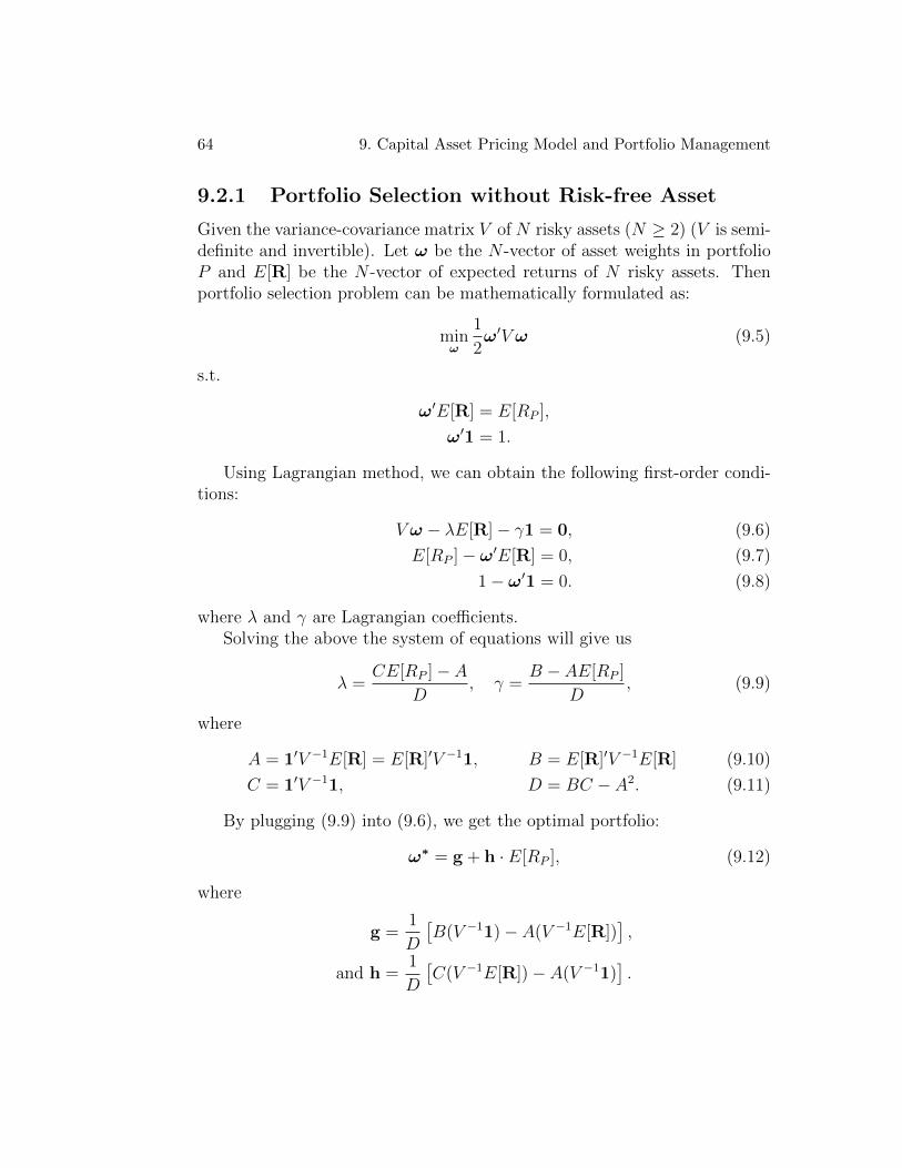
64 9. Capital Asset Pricing Model and Portfolio Management

9.2.1 Portfolio Selection without Risk-free Asset

Given the variance-covariance matrix V of N risky assets (N ≥ 2) (V is semi-definite and invertible). Let ω be the N -vector of asset weights in portfolioP and E[R] be the N -vector of expected returns of N risky assets. Thenportfolio selection problem can be mathematically formulated as:

minω

1

2ω′V ω (9.5)

s.t.

ω′E[R] = E[RP ],

ω′1 = 1.

Using Lagrangian method, we can obtain the following first-order condi-tions:

V ω − λE[R]− γ1 = 0, (9.6)

E[RP ]− ω′E[R] = 0, (9.7)

1− ω′1 = 0. (9.8)

where λ and γ are Lagrangian coefficients.Solving the above the system of equations will give us

λ =CE[RP ]− A

D, γ =

B − AE[RP ]

D, (9.9)

where

A = 1′V −1E[R] = E[R]′V −11, B = E[R]′V −1E[R] (9.10)

C = 1′V −11, D = BC − A2. (9.11)

By plugging (9.9) into (9.6), we get the optimal portfolio:

ω∗ = g + h · E[RP ], (9.12)

where

g =1

D

[B(V −11)− A(V −1E[R])

],

and h =1

D

[C(V −1E[R])− A(V −11)

].

9.2. Portfolio Management 65

Notations: Any optimal portfolio which can be represented by (9.12) isalso called frontier portfolio, while the set of all frontier portfolios is namedas portfolio frontier. Or equivalently, portfolio frontier is the curve of allfrontier portfolios.

In two-dimensional case, if |ρ| 6= 1 (equivalent condition for matrix V tobe non-singular), then it’s trivial since two constraint conditions in (9.5) canuniquely determine the weights ω and so the variance. Let’s consider twoextreme cases:

1. ρ = 1. Obviously, the volatility of the portfolio is given by

σP = ω1σ1 + ω2σ2,

which is a linear relationship.

2. ρ = −1. Similarly, we have

σP = |ω1σ1 − ω2σ2|.

Since the expected return of portfolio is linear all the time, we then drawthe expected return-volatility figure for portfolio when ρ = ±1. Notice thatFigure 9.1 doesn’t consider short-selling.

Figure 9.1: Expected return-volatility Figure when ρ = ±1

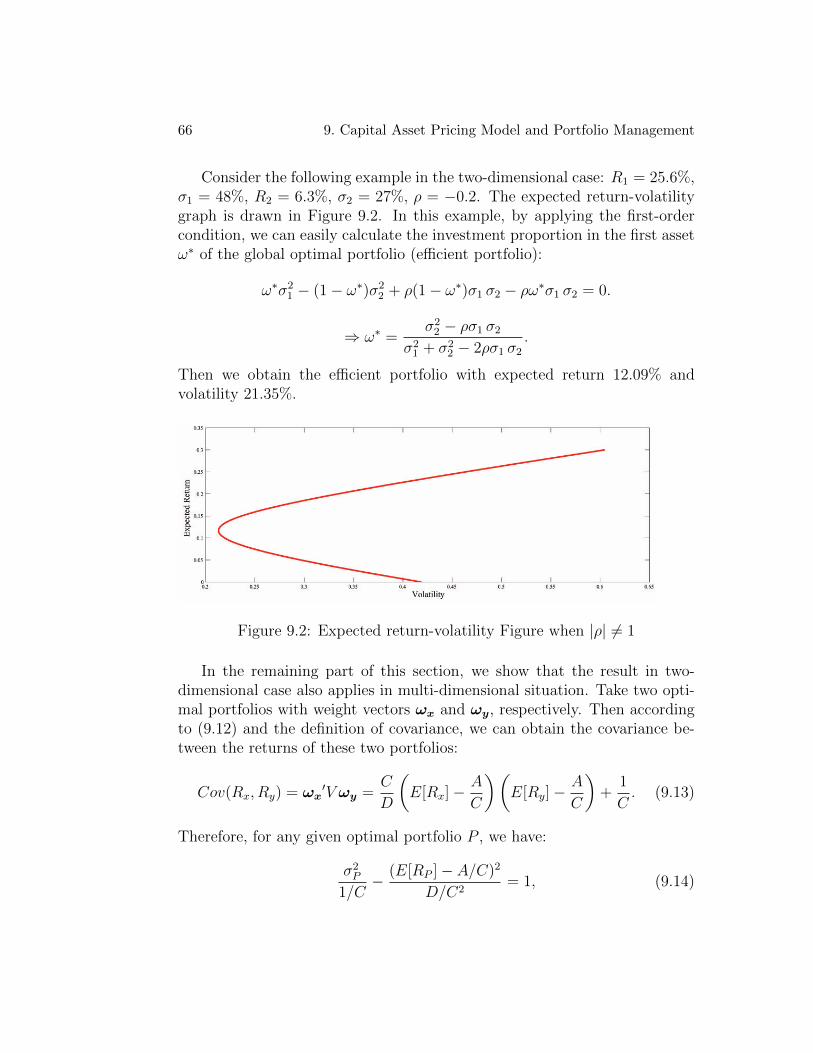
66 9. Capital Asset Pricing Model and Portfolio Management

Consider the following example in the two-dimensional case: R1 = 25.6%,σ1 = 48%, R2 = 6.3%, σ2 = 27%, ρ = −0.2. The expected return-volatilitygraph is drawn in Figure 9.2. In this example, by applying the first-ordercondition, we can easily calculate the investment proportion in the first assetω∗ of the global optimal portfolio (efficient portfolio):

ω∗σ21 − (1− ω∗)σ2

2 + ρ(1− ω∗)σ1 σ2 − ρω∗σ1 σ2 = 0.

⇒ ω∗ =σ2

2 − ρσ1 σ2

σ21 + σ2

2 − 2ρσ1 σ2

.

Then we obtain the efficient portfolio with expected return 12.09% andvolatility 21.35%.

Figure 9.2: Expected return-volatility Figure when |ρ| 6= 1

In the remaining part of this section, we show that the result in two-dimensional case also applies in multi-dimensional situation. Take two opti-mal portfolios with weight vectors ωx and ωy, respectively. Then accordingto (9.12) and the definition of covariance, we can obtain the covariance be-tween the returns of these two portfolios:

Cov(Rx, Ry) = ωx′V ωy =

C

D

(E[Rx]− A

C

)(E[Ry]−

A

C

)+

1

C. (9.13)

Therefore, for any given optimal portfolio P , we have:

σ2P

1/C− (E[RP ]− A/C)2

D/C2= 1, (9.14)

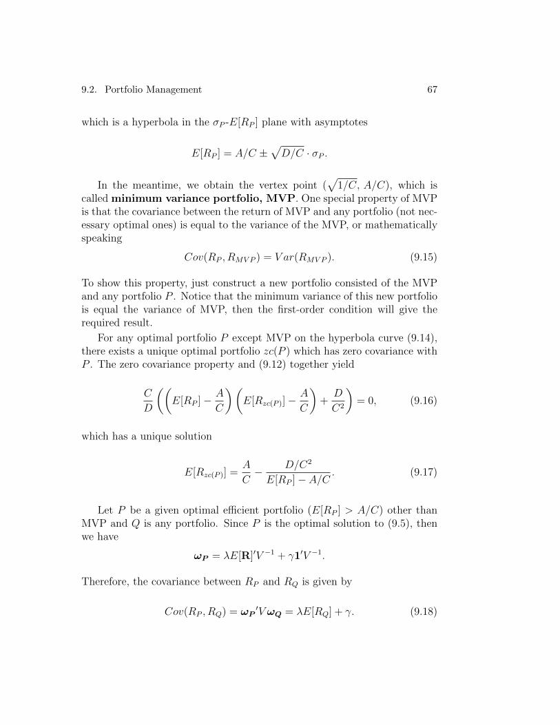
9.2. Portfolio Management 67

which is a hyperbola in the σP -E[RP ] plane with asymptotes

E[RP ] = A/C ±√D/C · σP .

In the meantime, we obtain the vertex point (√

1/C, A/C), which iscalled minimum variance portfolio, MVP. One special property of MVPis that the covariance between the return of MVP and any portfolio (not nec-essary optimal ones) is equal to the variance of the MVP, or mathematicallyspeaking

Cov(RP , RMV P ) = V ar(RMV P ). (9.15)

To show this property, just construct a new portfolio consisted of the MVPand any portfolio P . Notice that the minimum variance of this new portfoliois equal the variance of MVP, then the first-order condition will give therequired result.

For any optimal portfolio P except MVP on the hyperbola curve (9.14),there exists a unique optimal portfolio zc(P ) which has zero covariance withP . The zero covariance property and (9.12) together yield

C

D

((E[RP ]− A

C

)(E[Rzc(P )]−

A

C

)+D

C2

)= 0, (9.16)

which has a unique solution

E[Rzc(P )] =A

C− D/C2

E[RP ]− A/C. (9.17)

Let P be a given optimal efficient portfolio (E[RP ] > A/C) other thanMVP and Q is any portfolio. Since P is the optimal solution to (9.5), thenwe have

ωP = λE[R]′V −1 + γ1′V −1.

Therefore, the covariance between RP and RQ is given by

Cov(RP , RQ) = ωP′V ωQ = λE[RQ] + γ. (9.18)

68 9. Capital Asset Pricing Model and Portfolio Management

By plugging in (9.9) and re-arranging (9.18), we obtain

E[RQ] =AE[RP ]−BC E[RP ]− A

+ Cov(RP , RQ)D

C E[RP ]− A

=A

C− D/C2

E[RP ]− A/C

+Cov(RP , RQ)

σ2P

[1

C+

(E[RP ]− A/C)2

D/C

]D

C E[RP ]− A

= E[Rzc(P )] + βPQ

(E[RP ]− A

C+

D/C2

E[RP ]− A/C

)= (1− βP

Q)E[Rzc(P )] + βPQE[RP ] (9.19)

Recall the fact that zc(zc(P )) = P , so the above equality can be rewrittenas

E[RQ] = (1− βzc(P )Q )E[RP ] + β

zc(P )Q E[Rzc(P )]. (9.20)

Combining (9.19) and (9.20), we can see that

1− βPQ = β

zc(P )Q (9.21)

andE[RQ] = β

zc(P )Q E[Rzc(P )] + βP

QE[RP ]. (9.22)

9.2.2 Portfolio Selection with Risk-free Asset

In the section, we have N+1 assets in our market. We still use N-dimensionalvector ω denote the weights of risky assets in the portfolio. Since risk-freeasset has no uncertainty, which means it doesn’t contribute anything to thevolatility of the portfolio, then the problem (9.5) is modified as

minω

1

2ω′V ω (9.23)

s.t. ω′E[R] + (1− ω′1)Rf = E[RP ].

Similarly, by using Lagrangian method, we can obtain the first-order con-dition (which gives the optimal solution due to the semi definite property ofV )

V ω = λ(E[R]−Rf1)

E[RP ] = Rf + ω′(E[R]−Rf1)

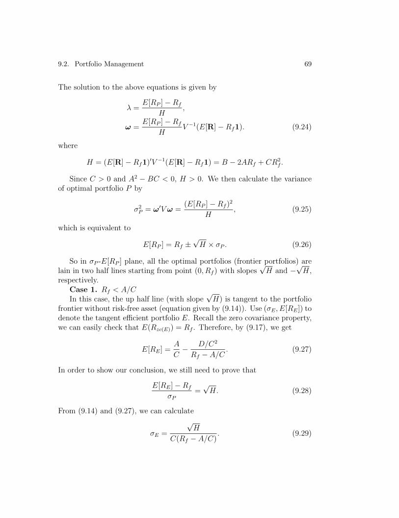
9.2. Portfolio Management 69

The solution to the above equations is given by

λ =E[RP ]−Rf

H,

ω =E[RP ]−Rf

HV −1(E[R]−Rf1). (9.24)

where

H = (E[R]−Rf1)′V −1(E[R]−Rf1) = B − 2ARf + CR2f .

Since C > 0 and A2 − BC < 0, H > 0. We then calculate the varianceof optimal portfolio P by

σ2P = ω′V ω =

(E[RP ]−Rf )2

H, (9.25)

which is equivalent to

E[RP ] = Rf ±√H × σP . (9.26)

So in σP -E[RP ] plane, all the optimal portfolios (frontier portfolios) arelain in two half lines starting from point (0, Rf ) with slopes

√H and −

√H,

respectively.Case 1. Rf < A/CIn this case, the up half line (with slope

√H) is tangent to the portfolio

frontier without risk-free asset (equation given by (9.14)). Use (σE, E[RE]) todenote the tangent efficient portfolio E. Recall the zero covariance property,we can easily check that E(Rzc(E)) = Rf . Therefore, by (9.17), we get

E[RE] =A

C− D/C2

Rf − A/C. (9.27)

In order to show our conclusion, we still need to prove that

E[RE]−Rf

σP=√H. (9.28)

From (9.14) and (9.27), we can calculate

σE =

√H

C(Rf − A/C). (9.29)

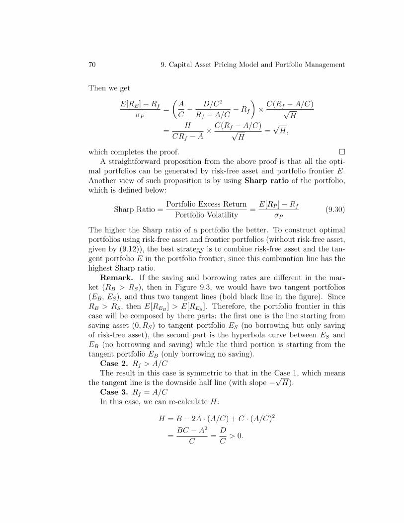
70 9. Capital Asset Pricing Model and Portfolio Management

Then we get

E[RE]−Rf

σP=

(A

C− D/C2

Rf − A/C−Rf

)× C(Rf − A/C)√

H

=H

CRf − A× C(Rf − A/C)√

H=√H,

which completes the proof. A straightforward proposition from the above proof is that all the opti-

mal portfolios can be generated by risk-free asset and portfolio frontier E.Another view of such proposition is by using Sharp ratio of the portfolio,which is defined below:

Sharp Ratio =Portfolio Excess Return

Portfolio Volatility=E[RP ]−Rf

σP(9.30)

The higher the Sharp ratio of a portfolio the better. To construct optimalportfolios using risk-free asset and frontier portfolios (without risk-free asset,given by (9.12)), the best strategy is to combine risk-free asset and the tan-gent portfolio E in the portfolio frontier, since this combination line has thehighest Sharp ratio.

Remark. If the saving and borrowing rates are different in the mar-ket (RB > RS), then in Figure 9.3, we would have two tangent portfolios(EB, ES), and thus two tangent lines (bold black line in the figure). SinceRB > RS, then E[REB

] > E[RES]. Therefore, the portfolio frontier in this

case will be composed by there parts: the first one is the line starting fromsaving asset (0, RS) to tangent portfolio ES (no borrowing but only savingof risk-free asset), the second part is the hyperbola curve between ES andEB (no borrowing and saving) while the third portion is starting from thetangent portfolio EB (only borrowing no saving).

Case 2. Rf > A/CThe result in this case is symmetric to that in the Case 1, which means

the tangent line is the downside half line (with slope −√H).

Case 3. Rf = A/CIn this case, we can re-calculate H:

H = B − 2A · (A/C) + C · (A/C)2

=BC − A2

C=D

C> 0.

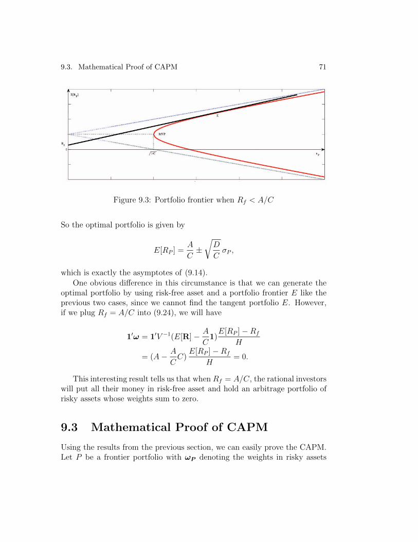
9.3. Mathematical Proof of CAPM 71

Figure 9.3: Portfolio frontier when Rf < A/C

So the optimal portfolio is given by

E[RP ] =A

C±√D

CσP ,

which is exactly the asymptotes of (9.14).

One obvious difference in this circumstance is that we can generate theoptimal portfolio by using risk-free asset and a portfolio frontier E like theprevious two cases, since we cannot find the tangent portfolio E. However,if we plug Rf = A/C into (9.24), we will have

1′ω = 1′V −1(E[R]− A

C1)E[RP ]−Rf

H

= (A− A

CC)

E[RP ]−Rf

H= 0.

This interesting result tells us that when Rf = A/C, the rational investorswill put all their money in risk-free asset and hold an arbitrage portfolio ofrisky assets whose weights sum to zero.

9.3 Mathematical Proof of CAPM

Using the results from the previous section, we can easily prove the CAPM.Let P be a frontier portfolio with ωP denoting the weights in risky assets

72 9. Capital Asset Pricing Model and Portfolio Management

while Q is any portfolio (may not be a frontier one) and weights vector ωQ.Furthermore, we assume E[RP ] 6= Rf . Then we have

Cov(RP , RQ) = ωQ′V ωP

= ωQ′(E[R]−Rf1)

E[RP ]−Rf

H

=(E[RQ]−Rf )(E[RP ]−Rf )

H. (9.31)

The above equality can be rearranged as

E[RQ]−Rf =Cov(RP , RQ)

(E[RP ]−Rf )/H

=Cov(RP , RQ)

(E[RP ]−Rf )2/H· (E[RP ]−Rf )

=Cov(RP , RQ)

σ2P

· (E[RP ]−Rf ) = βPQ(E[RP ]−Rf ), (9.32)

which directly gives CAPM (9.4) when we take market portfolio as P andassume market portfolio is a frontier portfolio.

Remark. In (9.31), there is a further assumption that ωQ′1 = 1, which

means portfolio Q doesn’t include risk-free asset. There are two propertieswhich make such assumption reasonable. The first property is that risk-freeasset satisfies CAPM since risk-free asset has zero beta while then the sec-ond is that CAPM is a linear model, so if risk-free asset and risky assetsall satisfy CAPM, then it’s obvious that CAPM will also hold for the linearcombination of all assets. Under such conclusion, we can always assume thatportfolio Q only contains all risky assets. Then from the arbitrariness ofportfolio Q, we know all risky assets will satisfy the CAPM (to check theith asset, just take ωQ = (0, 0, · · · , 1, · · · , 0)′, where 1 is the ith element ofvector).

Bibliography

[1] Jonathan Berk, Peter DeMarzo and David Stangeland. Corporate Fi-nance (Canadian Edition). Pearson Education Canada.

[2] Fischer Black and Myron Scholes. The pricing of options and corporateliabilities. Journal of Political Economy, 81, 637-54 (1973).

[3] Xiru Chen. Introductoin to Mathematical Statistics (ShuLiTongJiYin-Lun), Chinese Edition, 1997.

[4] Chi-fu Huang and Robert H. Litzenberger. Foundations For FinancialEconomics, Elsevier Science Publishing, 1997.

[5] John Hull. Options, Futures and Other Derivatives (7th edition), Pren-tice Hall, 2008.

[6] John Lintner. The Valuation of Risk Assets and the Selection of RiskyInvestments in Stock Portfolios and Capital Budgets. Review of Eco-nomics and Statistics, 47, 13-37 (1965).

[7] Andras Marosi. Lecture powerpoints of FIN 501, University of Alberta,2010 Fall.

[8] Harry Markowitz. Portfolio Selection. Journal of Finance, 7, 77-91.

[9] William Sharp. Capital Asset Prices: A Theory of Market Equilibriumunder Conditions of Risk. Journal of Finance, 19, 425-442 (1964).

[10] Steven Shreve. Stochastic Calculus for Finance (Volume I and II),Springer, 2005.

[11] http://en.wikipedia.org/wiki/Bond_finance.

73

74 BIBLIOGRAPHY

[12] http://en.wikipedia.org/wiki/Standard_deviation.

[13] http://en.wikipedia.org/wiki/Standard_error_(statistics).