Bigger is Better: Avoided Deforestation Offsets in the...
31
Bigger is Better: Avoided Deforestation Offsets in the Face of Adverse Selection Arthur van Benthem & Suzi Kerr Paper presented at the 55 th Annual National Conference of the Australia Agricultural & Resources Economics Society, Melbourne, Victoria, February 8-11, 2011
Transcript of Bigger is Better: Avoided Deforestation Offsets in the...
Bigger is Better: Avoided Deforestation Offsets in the Face of Adverse Selection
Arthur van Benthem & Suzi Kerr
Paper presented at the 55th Annual National Conference of the Australia Agricultural & Resources Economics Society, Melbourne, Victoria, February 8-11, 2011
Bigger is Better: Avoided Deforestation Offsets in the Face of
Adverse Selection∗
Arthur van Benthem†
Stanford University
Suzi Kerr‡
Motu Economic and Public Policy Research
Running title: Bigger is Better: Offsets and Adverse Selection
∗The authors would like to thank Adam Millard-Ball, Robert Heilmayr, Ruben Lubowski, Larry Goulder, andparticipants in seminars at Stanford University, NZARE, and the 2010 AIMES open science conference in Edinburghfor comments and suggestions. Suzi Kerr would like to thank the Program on Energy and Sustainable Developmentfor support while she was at Stanford. Van Benthem was supported by a Stanford Graduate Fellowship.†Department of Economics, Stanford University, 579 Serra Mall, Stanford, CA 94305, USA. E-mail:
[email protected]‡Corresponding author. Motu Economic and Public Policy Research and Stanford University, Level 1, 97 Cuba
Street, Wellington, New Zealand. Phone: (+64) 4 939 4250. Fax: (+64) 4 939 4251. E-mail: [email protected]
1
Abstract
Voluntary opt-in programs to reduce emissions in unregulated sectors or countries havespurred considerable discussion. Since any regulator will make errors in predicting baselinesand participants will self-select into the program, adverse selection will reduce efficiency andpossibly environmental integrity. In contrast, pure subsidies lead to full participation but requirelarge financial transfers. We present a simple model to analyze this trade-off between adverseselection and infra-marginal transfers. We find that increasing the scale of voluntary programsboth improves efficiency and reduces transfers. We show that discounting (paying less thanfull value for offsets) is inefficient and cannot be used to reduce the fraction of offsets thatare spurious while setting stringent baselines generally can. Both approaches reduce the costto the offsets buyer. The effects of two popular policy options are less favorable than manybelieve: Limiting the number of offsets that can be one-for-one exchanged with permits in acap-and-trade system will lower the offset price but also quality. Trading ratios between offsetsand allowances have ambiguous environmental effects if the cap is not properly adjusted. Thispaper frames the issues in terms of avoiding deforestation but the results are applicable to anyvoluntary offset program.
Keywords: deforestation, offsets, adverse selection, REDD, climate change policy, opt-in.
2
1 Introduction
Many reports (e.g. Stern, 2006) and key policy makers assert that avoiding deforestation is a key
short-run climate mitigation option because of the apparently low abatement costs (Kindermann
et al., 2008). Melillo et al. (2009) and Wise et al. (2009) both show that it is critically important
to price carbon in forests, especially if there are positive incentives for biofuels. Current estimates
of the forest carbon supply curve are based on either land use responses to commodity prices1, or
on estimates of the opportunity cost of land (e.g. Kindermann et al., 2006). These approaches
do not take into account the difficulty of designing effective policies to address deforestation in
developing countries, where most deforestation occurs (e.g. Andam et al., 2008; Pfaff et al., 2007).
They assume the application of efficient price-based policies, yet these are hard to achieve. Offset
programs have been shown to suffer from serious problems of spurious offsets and low effectiveness
as a result of adverse selection.2
This paper formally models voluntary price-based policy to avoid deforestation, examining the
implications of three key policy levers, project scale, price (“discounting” or trading ratios3), and
baseline stringency on the policy’s economic, environmental and distributional performance. We
consider three inter-related specific criteria: efficiency is determined by whether land goes to its
optimal use - land that yields high agricultural or timber returns should be cleared; land with
returns lower than the positive environmental externalities from the forest should not;4 value is
concerned with the average cost to industrialized countries of climate mitigation through avoided
deforestation; quality of offsets is measured as the percentage of offsets that are not spurious. If
quality is not taken into account through a more ambitious cap or fund it will reduce ’environmental
integrity’ (defined as the degree to which real global environmental gains are achieved as a result
of the policy).5
We use a microeconomic model of land use with a combination of analytical results and nu-
merical simulations to show that (1) baseline uncertainty in a voluntary program leads to reduced
1Examples include Kerr et al. (2002) for econometric estimates of transition to agricultural land use in response toprices, the MIT EPPA global general equilibrium model as used in Melillo et al. (2009), or Sathaye et al. (2006) fora partial equilibrium approach.
2Adverse selection is caused by a combination of two factors: a voluntary element (i.e., agents can choose whetheror not to opt in to the program) and asymmetric information about the baseline (i.e., the agents know more abouttheir true baseline than the regulator). Montero (2000), Fischer (2005) and Arguedas and van Soest (2009) establishtheoretical results for the effects of adverse selection on offsets programs. Montero (1999) gives the first empiricalevidence in the case of the US acid rain program. He and Morse (2010) and Millard-Ball (2010) explore similar issuesin the energy sector for the Clean Development Mechanism and for sectoral transportation caps respectively.
3In our model lowering the price is equivalent to requiring a trading ratio when offsets are used in a cap-and-tradesystem in which the cap can be adjusted to achieve the same global abatement. A 5:1 trading ratio is an 80% pricediscount.
4Higher efficiency will be associated with more avoided deforestation up to a limit. Avoided deforestation may alsobe of independent interest because of associated benefits such as flood protection, water quality and biodiversity.
5A lower quality of offset also has equity implications because a higher share of the gains from mitigation will go toactors who have not really mitigated.
3
efficiency and spurious offsets, but increasing the required scale of projects that can participate mit-
igates these problems; (2) ’discounting’ offsets reduces the quality of offsets and reduces efficiency
but generally lowers payments per hectare; therefore, the only rationale for offset discounting is
to increase the value to industrialized countries per dollar of transfers to offset sellers; (3) more
stringent baselines also reduce efficiency but generally improve the quality of offsets while also
improving value for money.
Actual price-based policies for climate mitigation in developing countries are still mostly limited
to offset programs. Examples include the payments for ecosystem services program in Costa Rica
(Sanchez et al., 2007) and the Clean Development Mechanism, where actors are given credit for
forest remaining above an estimated and assigned baseline, or for emission reductions below a
baseline. Several designs have been proposed for an international program to reduce deforestation.6
Some are beginning to be implemented on a wider scale - notably Norway’s innovative contracts
with Guyana, Brazil and Indonesia.7 All proposed policies have elements of offsets in their design
and face a tradeoff between efficiency and the desire of the funders of such programs to get the best
value for the money they spend.8 It has been suggested that programs should discount the price
per hectare paid to landowners, or increase their assigned baseline, to ”correct” for spurious offsets
and the resulting loss of environmental integrity.
Our paper can be interpreted as an analysis of either adding avoided deforestation to a broader
cap-and-trade market, or as an international fund used to pay for avoided deforestation to supple-
ment a separate cap on other emissions. Both programs involve a baseline level of forest and provide
rewards relative to that. In a cap-and-trade market these rewards would be offsets valued at the
market price, whereas in the fund these rewards would be dollars. In both programs industrialized
countries pay for the reductions that are achieved in developing countries. These two approaches
are equivalent under the following assumptions. First, the rewards must be the same per unit of
avoided deforestation. To set fund payouts that meet this assumption requires that the aggregate
marginal cost functions of the forest landowners are known so that the market price in the cap-
and-trade system can be predicted accurately. Second, the cap-and-trade market emissions cap and
the level of the fund can be adjusted so that regardless of which approach is used, both the global
environmental outcome and the permit price are identical. That is, the fund level would need to
be set such that the environmental gains it achieved were equal to the difference in environmental
6These efforts are most recently referred to as REDD - Reducing Emissions from Deforestation and Degradation.A plethora of reports and edited volumes explore the issues associated with the design of REDD and its successorREDD+. See Angelsen (2008), Chomitz (2007), Plantinga and Richards (2008) for recent discussions of the challenges.Strand (2010) points out that offset programs can lead to increased emissions in the short run from countries thathave not yet opted in, but use lax environmental standards to increase their baseline emissions.
7For example see Government of Kingdom of Norway and Government of the Republic of Indonesia (2010).8Several studies provide evidence on the efficiency effects of adverse selection in the context of Costa Rican deforestation(Kerr et al., 2004; Robalino et al., 2008; Sanchez et al., 2007). Busch et al. (2009) focus on the global efficiencyeffects of different baselines (reference levels) in a deforestation program. Wara and Victor (2008) explore the extentof spurious credits in the Clean Development Mechanism.
4
gains between the environmental cap of the larger broad cap and trade system (including avoided
deforestation) and the original cap and trade market (excluding avoided deforestation).9
Our presentation focuses on deforestation but the results are equally applicable to many other
internationally funded mitigation options in developing countries, as well as wider applications of
voluntary offset programs.
The remainder of this paper is organized as follows. Section 2 presents a simple model of
voluntary deforestation policy that operates first at the level of individual plots, and then for larger
scales. This demonstrates the trade-off between efficiency loss from adverse selection and the level
of transfers, and analyzes how the three policy criteria are affected by the shapes of the distributions
of land returns and observation errors. Section 3 discusses how the potential objectives are affected
by three different policy choices: increasing the scale required for participation, changing the carbon
payment (equivalent to “discounting offsets”) and changing the generosity of the assigned baseline.
Section 4 concludes and summarizes the main policy implications.
2 A Simple Model of Voluntary Opt-In
2.1 Efficient subsidies versus baselines with adverse selection
Consider a continuum of plots of forested land, indexed by i. Decisions on each plot are independent.
Landowners decide to either clear fully or keep the forest. Landowners will clear their forest if the net
return from deforesting ri (e.g. agricultural plus timber revenues minus clearing costs) exceeds any
payment pc to maintain forest. Landowner i knows ri with certainty. The marginal environmental
externality from deforestation is defined as δ.10 Returns ri are distributed across i with density fr.
The simplest policy would be to offer a subsidy equal to pc per plot that remains forested, where
pc = δ. All landowners with ri ≤ pc will accept the subsidy and not deforest but only landowners
with 0 ≤ ri ≤ pc will actually change their behavior; landowners with ri > pc will (efficiently)
9Suppose industrialized countries (ICs) have a joint emissions cap that requires them to undertake abatement of A.Total abatement cost (TAC) is the integral under the IC marginal abatement cost curve up to A. The market priceof pollution equals p∗. ICs could use the fund to achieve n further units of abatement (and pay for m infra-marginal,or “spurious”, units), at price per unit pc which may be lower than p∗. Total global abatement would be A + n,where n is a function of pc.
Analogous to the fund, ICs could purchase n+m offsets from developing countries (DCs) at price pc. This, however,would not be a fair comparison. Under the fund, the global abatement equals A + n. Using offsets, and with notrading ratio, global abatement will be A −m. The environmental outcome is worse than without offsets (and pcwould be lower). To correct this, ICs must increase their joint abatement target to A + n + m. This ensures that,after n+m offsets are purchased from DCs, the IC mitigation effort is back at A and the pollution price at p∗. Globalabatement is now also A+ n.
If a trading ratio t : 1 is applied, under offsets global abatement will be A+ (t− 1)n−m, where n and m are nowfunctions of t. This could be higher or lower than A+ n. Again an adjustment to the joint abatement target wouldbe needed to make them equivalent.
10We implicitly assume that the amount of carbon per hectare of forest is constant. This could be relaxed with no lossof generality.
5
deforest.11 The change in economic surplus ∆Seff from this efficient policy relative to no policy
equals
Efficiency gain = ∆Seff =
∫ pc
0(pc − r) fr (r) dr (1)
This achieves efficient deforestation but requires a large transfer of resources
Total transfer = TT = pc
∫ pc
−∞fr (r) dr (2)
The total amount of avoided deforestation is
Avoided deforestation = AD =
∫ pc
0fr (r) dr (3)
The average cost (AC = TT/AD) to industrialized countries of climate mitigation through
avoided deforestation summarizes the value of the program to ICs. Under the subsidy, the value is
low (average cost is high) if many plots of land have negative returns and so would not have been
cleared even without the subsidy.
To avoid large transfers, a second policy option is a voluntary deforestation program that will pay
participants an amount pc for each hectare of forest exceeding an assigned baseline.12 Landowners
know their true forest baselines BLi:
BLi =
{1 if ri ≤ 0
0 if ri > 0
}(4)
If the regulator observes ri, the efficient solution is achieved by assigning each landowner i the
true baseline BLi(ri). If BLi = 1 (no deforestation), no payment will be made and the forest will
remain intact. If BLi = 0 (full deforestation) and 0 ≤ ri ≤ pc, the landowner will opt in and choose
not to deforest. If BLi = 0 and ri > pc, the landowner will deforest and forego the payment pc. If
11The ri may be interdependent. General equilibrium effects mean one landowner’s decision whether to deforest willalter returns for others. This could operate through leakage where a landowner who does not deforest reduces supplyof timber and/or food which affect prices for those. It could also occur if clearing involves investment in localinfrastructure, or induces local service provision or labor supply that make clearing more attractive for neighboringparcels. These effects could also occur if a local government is the entity avoiding deforestation. For example, afarmer education program to raise yields on existing crop land with a new technology or practice could spill overto more intensive production in neighboring communities if the information spreads. This could either increase ordecrease ri. fr could be thought of as an ex-post distribution of returns when a new set of equilibrium land uses isreached.
12If it were practically feasible, a policy that sets pc = ri would reduce transfers even further. In a recent paper, Masonand Plantinga (2010) describe a model in which the regulator has the option to provide landowners with a menuof two-part contracts, which consist of a lump-sum payment from the landowner to the regulator and a “per unitof forest” back to the landowner. Under certain conditions, these are type-revealing, where an ex-ante unobserved“type” corresponds to a marginal opportunity cost curve of keeping a fraction of the land forested. A similar approachto maximize the benefits to the developed country funders in an environmental transfer program was developed inKerr (1995). Our model does not consider this option.
6
pc = δ, the remaining deforestation is efficient. Efficiency and avoided deforestation are the same
as in (1) and (3) but the total transfer is lower by the amount in (5) and hence the average cost
(value) is lower (higher). This policy dominates the subsidy if transfers are costly.
Decrease in TT relative to subsidy = pc
0∫−∞
fr (r) dr (5)
In practice, however, the regulator cannot observe ri, but instead observes r̂i = ri + εi. The
observation error εi has density fε ∼ (0, σε), is assumed to be symmetric around 0 and independent
of fr. The predicted baselines are
B̂Li =
{1 if r̂i ≤ 0
0 if r̂i > 0
}(6)
What happens if the government assigns baseline B̂Li? When (ri > 0, r̂i > 0) or (ri ≤ 0, r̂i ≤ 0),
the assigned baseline coincides with the true baseline. The landowner will make the socially efficient
decision. However, if (ri > 0, r̂i ≤ 0), the assigned baseline is 1 but the true baseline is 0. The
landowner would have deforested the plot in the true baseline, but gets assigned an unfavorable
“no deforestation” baseline. Hence, the landowner will not participate in the scheme. This leads to
an efficiency loss if 0 ≤ ri ≤ pc = δ, since the landowner will now deforest while he would not have
done so had his baseline been correctly assigned and he had participated in the scheme. Relative
to the efficient outcome in (1) the efficiency loss caused by adverse selection equals
pc∫0
(pc − r)
−r∫−∞
fε (ε) dε
fr (r) dr (7)
The amount of avoided deforestation will fall by
pc∫0
−r∫−∞
fε (ε) dε
fr (r) dr (8)
Finally, consider the case where (ri ≤ 0, r̂i > 0). These landowners would have kept their forest,
but now get assigned a full deforestation baseline. This will not affect their behavior, but it implies
an additional infra-marginal transfer pc. The total transfer (TT ) is now lower than the subsidy
amount (2). TT is given by the sum of marginal transfers (MT ) and infra-marginal transfers (IT ).
The former are the payments made to landowners that change their decision as a result of the
policy and do not deforest. The latter are payments to landowners that would not have deforested
without the policy, but get assigned a favorable full deforestation baseline and will therefore opt
7
in.13
TT = MT + IT
= pcpc∫0
(∞∫−rfε (ε) dε
)fr (r) dr + pc
0∫−∞
(∞∫−rfε (ε) dε
)fr (r) dr
(9)
The amount of avoided deforestation is reduced relative to both the subsidy and the full infor-
mation voluntary program (both given by (3)). Total transfers are lower than under the subsidy
(2), but can be either higher or lower than under the full information program (5).14 The effect
of adverse selection on average cost is theoretically ambiguous relative to the subsidy but clearly
higher relative to the full information voluntary program.
To obtain intuition for this ambiguity, we use the decomposition in (9) to write AC as
pc
1 +
0∫−∞
(∞∫−rfε (ε) dε
)fr (r) dr
pc∫0
(∞∫−rfε (ε) dε
)fr (r) dr
= pc
(1 +
OS
AD
)(10)
where OS denotes the amount of infra-marginal forest credited, or offsets that are “spurious”.
Moving from a subsidy to a voluntary program reduces OS but also lowers AD. For most realistic
distributions (described in Section 2.2) the reduction in OS is larger than the reduction in AD, so
AC would fall. We use the fraction of offsets that are spurious (FOS = OS/AD) as a measure of
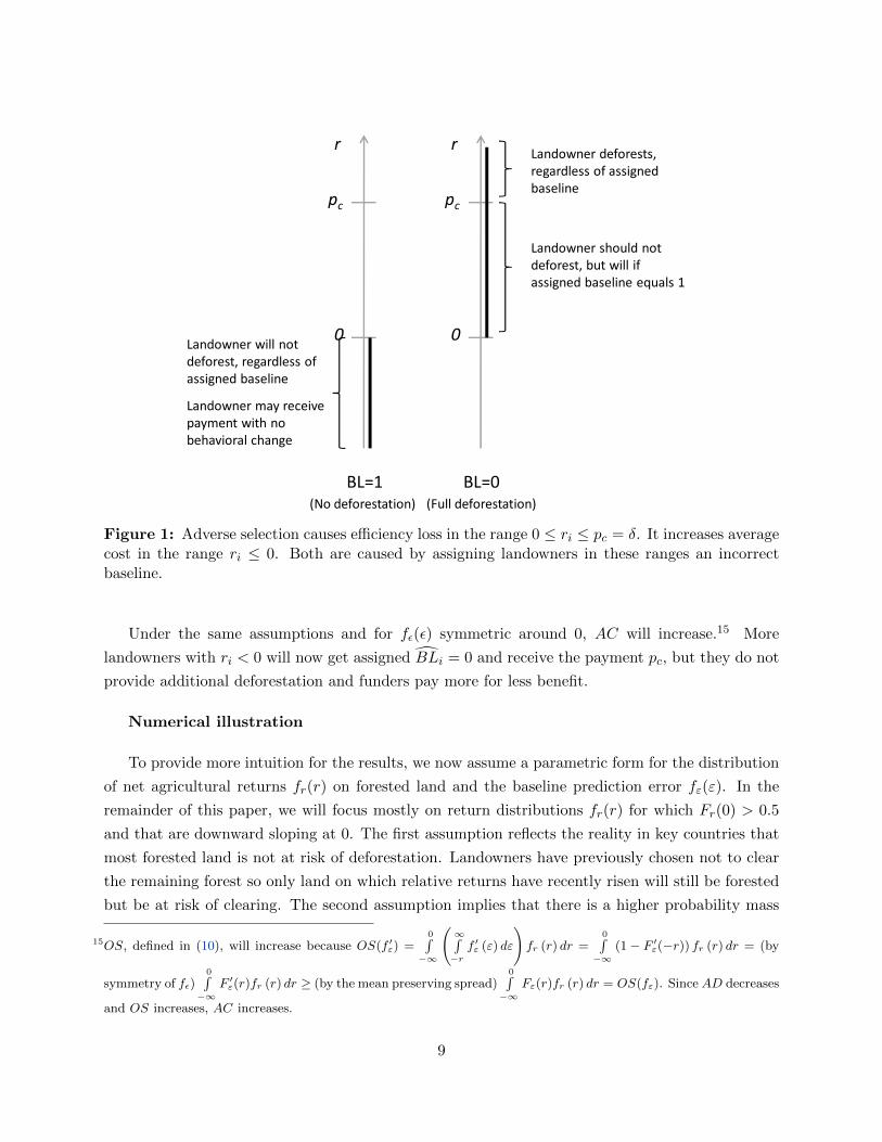
the offset quality. The cases described above are summarized in Figure 1.
2.2 The impacts of observation error distributions on policy objectives
The tradeoff between efficiency and value depends on the distributions of observation errors. We
now analyze the impact of observation error variance on our three policy objectives: economic
efficiency, value (AC) and offset quality (FOS; a measure of the environmental integrity of the
program).
Equation (7) shows that any change in fε(ε) that increases the probability mass in the range
[−∞,−ri], where 0 ≤ ri ≤ pc, will increase the efficiency loss from adverse selection (assuming
pc = δ) and decrease avoided deforestation. A mean preserving spread such that F ′ε(x) ≥ Fε(x)
∀x < 0 is sufficient. If the distribution of errors is normal, an increase in variance will generate
such a mean preserving spread.
13In a cap-and-trade program, infra-marginal transfers would be spurious or non-additional credits.14From (2) and (9), it follows trivially that TT (baseline) < TT (subsidy). However, TT (baseline) is unsigned relative
to TT (full information), because IT (baseline) > IT (full information) = 0, but MT (baseline) < MT (fullinformation). Generally, TT (baseline) > TT (full information). However, if, for example, fr(r) has no densitybelow 0, TT (baseline) < TT (full information).
8
BL=1 BL=0
r r
pc pc
0 0
Landowner deforests,
regardless of assigned
baseline
Landowner should not
deforest, but will if
assigned baseline equals 1
Landowner will not
deforest, regardless of
assigned baseline
Landowner may receive
payment with no
behavioral change
Figure 1
(No deforestation) (Full deforestation)
Figure 1: Adverse selection causes efficiency loss in the range 0 ≤ ri ≤ pc = δ. It increases averagecost in the range ri ≤ 0. Both are caused by assigning landowners in these ranges an incorrectbaseline.
Under the same assumptions and for fε(ε) symmetric around 0, AC will increase.15 More
landowners with ri < 0 will now get assigned B̂Li = 0 and receive the payment pc, but they do not
provide additional deforestation and funders pay more for less benefit.
Numerical illustration
To provide more intuition for the results, we now assume a parametric form for the distribution
of net agricultural returns fr(r) on forested land and the baseline prediction error fε(ε). In the
remainder of this paper, we will focus mostly on return distributions fr(r) for which Fr(0) > 0.5
and that are downward sloping at 0. The first assumption reflects the reality in key countries that
most forested land is not at risk of deforestation. Landowners have previously chosen not to clear
the remaining forest so only land on which relative returns have recently risen will still be forested
but be at risk of clearing. The second assumption implies that there is a higher probability mass
15OS, defined in (10), will increase because OS(f ′ε) =0∫−∞
(∞∫−rf ′ε (ε) dε
)fr (r) dr =
0∫−∞
(1− F ′ε(−r)) fr (r) dr = (by
symmetry of fε)0∫−∞
F ′ε(r)fr (r) dr ≥ (by the mean preserving spread)0∫−∞
Fε(r)fr (r) dr = OS(fε). Since AD decreases
and OS increases, AC increases.
9
for returns just below zero than for returns just above zero, which intensifies the tradeoff between
efficiency and reducing transfers and, in particular, infra-marginal rewards.
With no shocks, all land with positive returns would already have been cleared without any
policy while no land with negative returns would have been cleared. Hence, there will be positive
probability mass below zero and no mass above zero and the assumption trivially holds. Deforesta-
tion occurs because the returns distribution shifts over time. If this shift, driven by, for example,
technology and local infrastructure change, has both a common and an idiosyncratic (e.g. normal
unbiased shock to each plot) element we would still expect the second assumption to hold.16 The
density above zero will tend to be lower than below zero, since the tail of the normal distribution
implies a negative slope.
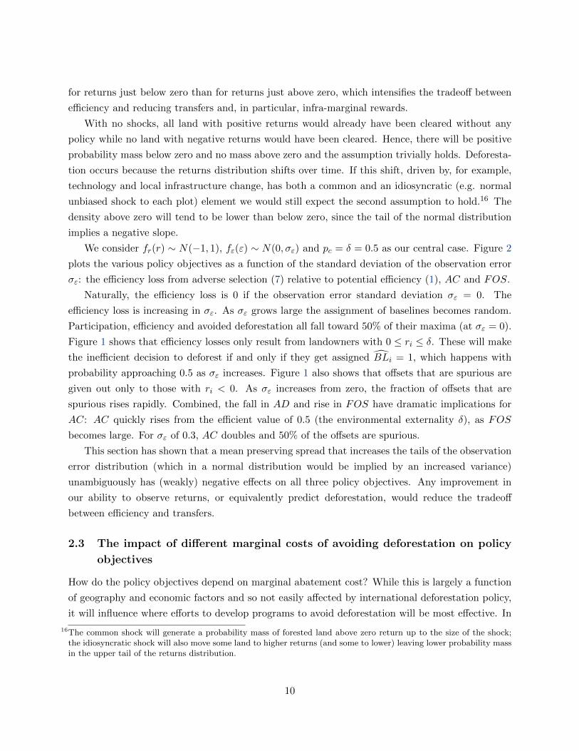
We consider fr(r) ∼ N(−1, 1), fε(ε) ∼ N(0, σε) and pc = δ = 0.5 as our central case. Figure 2
plots the various policy objectives as a function of the standard deviation of the observation error
σε: the efficiency loss from adverse selection (7) relative to potential efficiency (1), AC and FOS.
Naturally, the efficiency loss is 0 if the observation error standard deviation σε = 0. The
efficiency loss is increasing in σε. As σε grows large the assignment of baselines becomes random.
Participation, efficiency and avoided deforestation all fall toward 50% of their maxima (at σε = 0).
Figure 1 shows that efficiency losses only result from landowners with 0 ≤ ri ≤ δ. These will make
the inefficient decision to deforest if and only if they get assigned B̂Li = 1, which happens with
probability approaching 0.5 as σε increases. Figure 1 also shows that offsets that are spurious are
given out only to those with ri < 0. As σε increases from zero, the fraction of offsets that are
spurious rises rapidly. Combined, the fall in AD and rise in FOS have dramatic implications for
AC: AC quickly rises from the efficient value of 0.5 (the environmental externality δ), as FOS
becomes large. For σε of 0.3, AC doubles and 50% of the offsets are spurious.
This section has shown that a mean preserving spread that increases the tails of the observation
error distribution (which in a normal distribution would be implied by an increased variance)
unambiguously has (weakly) negative effects on all three policy objectives. Any improvement in
our ability to observe returns, or equivalently predict deforestation, would reduce the tradeoff
between efficiency and transfers.
2.3 The impact of different marginal costs of avoiding deforestation on policy
objectives
How do the policy objectives depend on marginal abatement cost? While this is largely a function
of geography and economic factors and so not easily affected by international deforestation policy,
it will influence where efforts to develop programs to avoid deforestation will be most effective. In
16The common shock will generate a probability mass of forested land above zero return up to the size of the shock;the idiosyncratic shock will also move some land to higher returns (and some to lower) leaving lower probability massin the upper tail of the returns distribution.
10
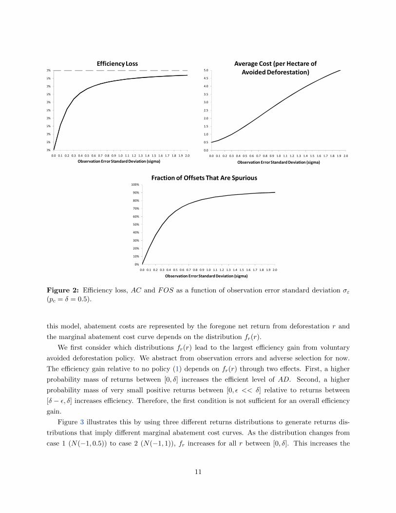
Figure 2
0%
5%
10%
15%
20%
25%
30%
35%
40%
45%
50%
0.0 0.1 0.2 0.3 0.4 0.5 0.6 0.7 0.8 0.9 1.0 1.1 1.2 1.3 1.4 1.5 1.6 1.7 1.8 1.9 2.0
Observation Error Standard Deviation (sigma)
Efficiency Loss
0.0
0.5
1.0
1.5
2.0
2.5
3.0
3.5
4.0
4.5
5.0
0.0 0.1 0.2 0.3 0.4 0.5 0.6 0.7 0.8 0.9 1.0 1.1 1.2 1.3 1.4 1.5 1.6 1.7 1.8 1.9 2.0
Observation Error Standard Deviation (sigma)
Average Cost (per Hectare of
Avoided Deforestation)
0%
10%
20%
30%
40%
50%
60%
70%
80%
90%
100%
0.0 0.1 0.2 0.3 0.4 0.5 0.6 0.7 0.8 0.9 1.0 1.1 1.2 1.3 1.4 1.5 1.6 1.7 1.8 1.9 2.0
Observation Error Standard Deviation (sigma)
Fraction of Offsets That Are Spurious
Figure 2: Efficiency loss, AC and FOS as a function of observation error standard deviation σε(pc = δ = 0.5).
this model, abatement costs are represented by the foregone net return from deforestation r and
the marginal abatement cost curve depends on the distribution fr(r).
We first consider which distributions fr(r) lead to the largest efficiency gain from voluntary
avoided deforestation policy. We abstract from observation errors and adverse selection for now.
The efficiency gain relative to no policy (1) depends on fr(r) through two effects. First, a higher
probability mass of returns between [0, δ] increases the efficient level of AD. Second, a higher
probability mass of very small positive returns between [0, ε << δ] relative to returns between
[δ − ε, δ] increases efficiency. Therefore, the first condition is not sufficient for an overall efficiency
gain.
Figure 3 illustrates this by using three different returns distributions to generate returns dis-
tributions that imply different marginal abatement cost curves. As the distribution changes from
case 1 (N(−1, 0.5)) to case 2 (N(−1, 1)), fr increases for all r between [0, δ]. This increases the
11
deforestation response at every positive price, by unambiguously lowering marginal abatement cost,
and hence increases the efficiency gain of the policy. The efficiency gain increases fourfold, while
AD increases fivefold. However, moving from case 2 to case 3 (Uniform(−3.6, 1.6)), fr increases
for r close to δ, but decreases for small r. AD increases by seven percent, but the efficiency gain
decreases by three percent. Hence, the relationship between avoided deforestation and the potential
efficiency gain is ambiguous.
Figure 3
-2 -1 1 2
0.2
0.4
0.6
0.8
f r
Case 1: σr
= 0.5
Case 2: σr
= 1.0
Case 3: uniform
δ
Notes: case 1: fr(r) ∼ N(−1, 0.5); case 2: fr(r) ∼ N(−1, 1); case 3:fr(r) ∼ Uniform(−3.6, 1.6). δ = pc = 0.5. fε(ε) ∼ N(0, 0.5).
Figure 3: The ambiguous relationship between returns distributions, avoided deforestation andefficiency.
Proposition 1. A returns distribution fr that generates more AD at pc = δ than f ′r does not
necessarily generate a higher efficiency gain.
Proof. By counterexample (Figure 3).17
17A more general counterexample can be constructed as follows. Consider a distribution fr that is downward sloping inthe interval r ∈ [0, pc = δ], and a distribution f ′r such that f ′r = fr(pc−r) for this interval and f ′r(r) = fr(r) elsewhere
in the domain. First, note thatpc∫0
f ′r (r) dr =pc∫0
fr (pc − r) dr =pc∫0
fr (r) dr. Second, since∞∫−rfε (ε) dε is increasing
in r, AD (f ′r) =pc∫0
(∞∫−rfε (ε) dε
)f ′r (r) dr >
pc∫0
(∞∫−rfε (ε) dε
)fr (r) dr = AD (fr). For example, consider fε(ε)) ∼
Uniform(−k, k) with k > pc. In that case,∞∫−rfε (ε) dε = 1
2
(1 + r
k
)for r ≤ pc. Hence, (pc − r)
(∞∫−rfε (ε) dε
)is
decreasing in r. Therefore, ∆S (f ′r) =pc∫0
(pc − r)
(∞∫−rfε (ε) dε
)f ′r (r) dr =
pc∫0
(pc − r)
(∞∫−rfε (ε) dε
)fr (pc − r) dr <
pc∫0
(pc − r)
(∞∫−rfε (ε) dε
)fr (r) dr = ∆S (fr), since f ′r(r) is increasing in r while fr(r) is decreasing in r and f ′r(0) =
fr(pc). Hence, AD can increase while efficiency decreases.
12
Note that sufficient conditions for efficiency to increase are f ′r(r) > fr(r) ∀r ∈ [0, pc = δ], or -
somewhat weaker -pc∫0
f ′r (r) dr >pc∫0
fr (r) dr ∀r ∈ [0, pc = δ].
Proposition 1 shows that stronger assumptions on fr and f ′r are needed to ensure an increase
in efficiency than an increase in AD: an increase in the (observation error-weighted) probability
mass between [0, δ] is sufficient for AD to increase, but not to guarantee increased efficiency. In
other words, a return distribution that leads to a higher amount of optimal avoided deforestation
does not necessarily lead to a greater increase in efficiency.
With observation errors, a change in the returns distribution also affects the likelihood of
spurious offsets: a less negatively (more positively) sloped distribution around zero yields fewer
spurious offsets. The combined effects on AD and spurious offsets determine the effect on AC.
Numerical illustration
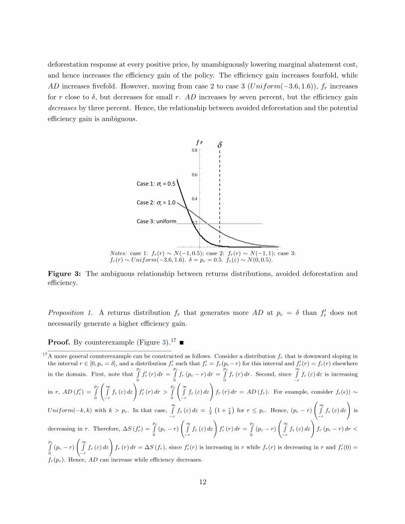
Figure 4 illustrates these effects using a numerical example similar to the previous one with
fr(r) ∼ N(−1, σr), fε(ε) ∼ N(0, σε), σε = 0.5, pc = δ = 0.5 and three different σr which alter
the relevant part of fr(r). Case 3 now corresponds to a N(−1, 2) returns distribution. Marginal
abatement cost unambiguously falls between case 1 and 2 while in case 3 it is higher than 2 for
some units and lower for others. Figure 4
0
0.5
1
1.5
2
2.5
3
3.5
4
4.5
5
0.00
0.01
0.02
0.03
0.04
0.05
0.06
0.07
0.0 0.1 0.2 0.3 0.4 0.5 0.6 0.7 0.8 0.9 1.0 1.1 1.2 1.3 1.4 1.5 1.6 1.7 1.8 1.9 2.0
Return Distribution Standard Deviation
Efficiency Gain Avoided Deforestation
Fraction of Offsets That Are Spurious (Sec. Axis) Average Cost (Sec. Axis)
Case 1: σr
= 0.5 Case 2: σr
= 1.0 Case 3: σr
= 2.0
Figure 4: Impact of changing fr(r) on the policy objectives, with pc = δ = 0.5 and σε = 0.5.
13
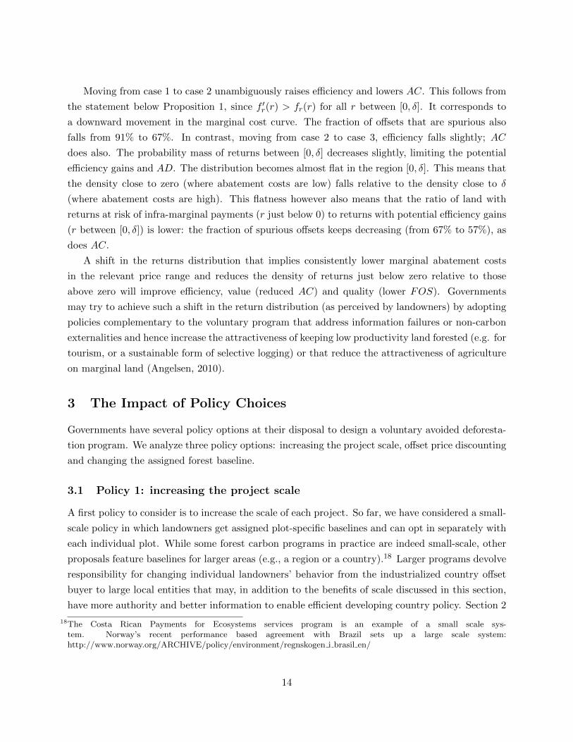
Moving from case 1 to case 2 unambiguously raises efficiency and lowers AC. This follows from
the statement below Proposition 1, since f ′r(r) > fr(r) for all r between [0, δ]. It corresponds to
a downward movement in the marginal cost curve. The fraction of offsets that are spurious also
falls from 91% to 67%. In contrast, moving from case 2 to case 3, efficiency falls slightly; AC
does also. The probability mass of returns between [0, δ] decreases slightly, limiting the potential
efficiency gains and AD. The distribution becomes almost flat in the region [0, δ]. This means that
the density close to zero (where abatement costs are low) falls relative to the density close to δ
(where abatement costs are high). This flatness however also means that the ratio of land with
returns at risk of infra-marginal payments (r just below 0) to returns with potential efficiency gains
(r between [0, δ]) is lower: the fraction of spurious offsets keeps decreasing (from 67% to 57%), as
does AC.
A shift in the returns distribution that implies consistently lower marginal abatement costs
in the relevant price range and reduces the density of returns just below zero relative to those
above zero will improve efficiency, value (reduced AC) and quality (lower FOS). Governments
may try to achieve such a shift in the return distribution (as perceived by landowners) by adopting
policies complementary to the voluntary program that address information failures or non-carbon
externalities and hence increase the attractiveness of keeping low productivity land forested (e.g. for
tourism, or a sustainable form of selective logging) or that reduce the attractiveness of agriculture
on marginal land (Angelsen, 2010).
3 The Impact of Policy Choices
Governments have several policy options at their disposal to design a voluntary avoided deforesta-
tion program. We analyze three policy options: increasing the project scale, offset price discounting
and changing the assigned forest baseline.
3.1 Policy 1: increasing the project scale
A first policy to consider is to increase the scale of each project. So far, we have considered a small-
scale policy in which landowners get assigned plot-specific baselines and can opt in separately with
each individual plot. While some forest carbon programs in practice are indeed small-scale, other
proposals feature baselines for larger areas (e.g., a region or a country).18 Larger programs devolve
responsibility for changing individual landowners’ behavior from the industrialized country offset
buyer to large local entities that may, in addition to the benefits of scale discussed in this section,
have more authority and better information to enable efficient developing country policy. Section 2
18The Costa Rican Payments for Ecosystems services program is an example of a small scale sys-tem. Norway’s recent performance based agreement with Brazil sets up a large scale system:http://www.norway.org/ARCHIVE/policy/environment/regnskogen i brasil en/
14
showed that observation errors in voluntary programs reduce efficiency and avoided deforestation,
value and quality. This section shows that increasing the required scale of each project in the
program mitigates these adverse consequences.
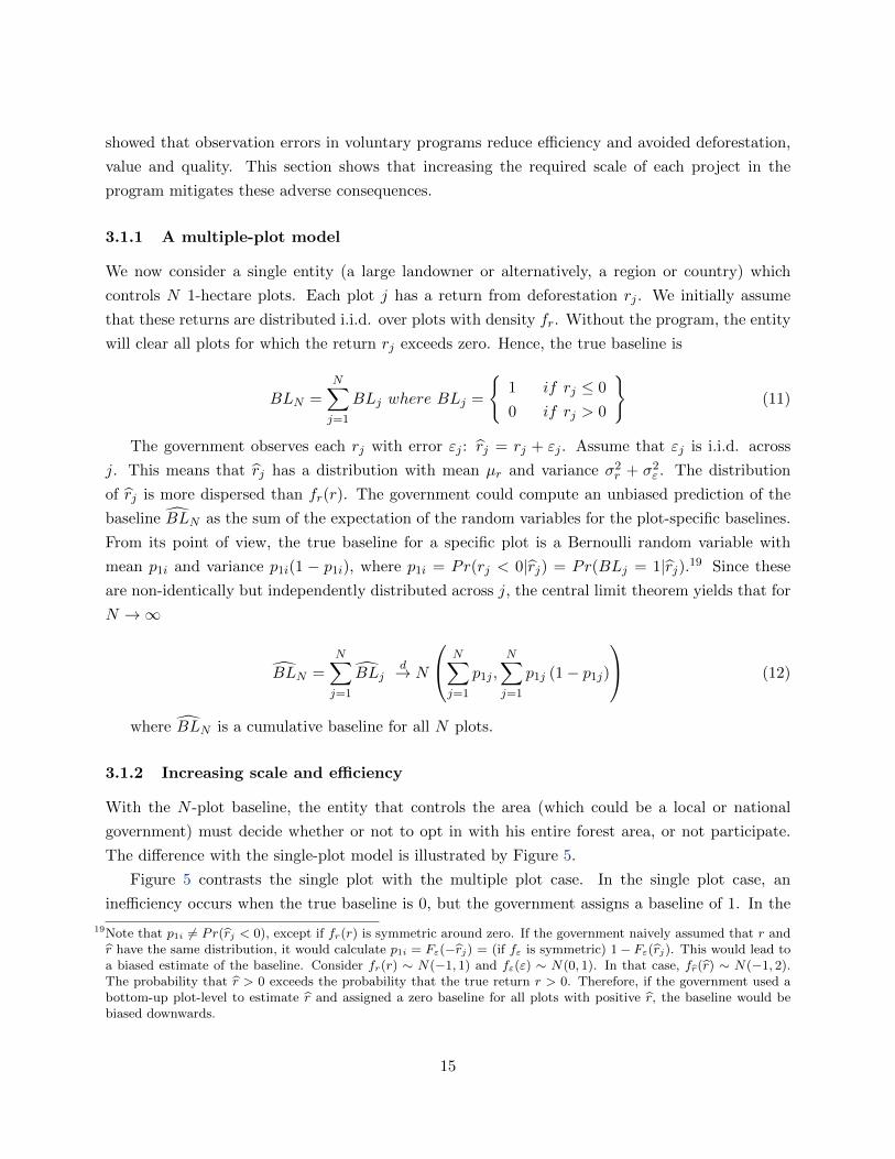
3.1.1 A multiple-plot model
We now consider a single entity (a large landowner or alternatively, a region or country) which
controls N 1-hectare plots. Each plot j has a return from deforestation rj . We initially assume
that these returns are distributed i.i.d. over plots with density fr. Without the program, the entity
will clear all plots for which the return rj exceeds zero. Hence, the true baseline is
BLN =N∑j=1
BLj where BLj =
{1 if rj ≤ 0
0 if rj > 0
}(11)
The government observes each rj with error εj : r̂j = rj + εj . Assume that εj is i.i.d. across
j. This means that r̂j has a distribution with mean µr and variance σ2r + σ2
ε . The distribution
of r̂j is more dispersed than fr(r). The government could compute an unbiased prediction of the
baseline B̂LN as the sum of the expectation of the random variables for the plot-specific baselines.
From its point of view, the true baseline for a specific plot is a Bernoulli random variable with
mean p1i and variance p1i(1 − p1i), where p1i = Pr(rj < 0|r̂j) = Pr(BLj = 1|r̂j).19 Since these
are non-identically but independently distributed across j, the central limit theorem yields that for
N →∞
B̂LN =N∑j=1
B̂Ljd→ N
N∑j=1
p1j ,N∑j=1
p1j (1− p1j)
(12)
where B̂LN is a cumulative baseline for all N plots.
3.1.2 Increasing scale and efficiency
With the N -plot baseline, the entity that controls the area (which could be a local or national
government) must decide whether or not to opt in with his entire forest area, or not participate.
The difference with the single-plot model is illustrated by Figure 5.
Figure 5 contrasts the single plot with the multiple plot case. In the single plot case, an
inefficiency occurs when the true baseline is 0, but the government assigns a baseline of 1. In the
19Note that p1i 6= Pr(r̂j < 0), except if fr(r) is symmetric around zero. If the government naively assumed that r andr̂ have the same distribution, it would calculate p1i = Fε(−r̂j) = (if fε is symmetric) 1− Fε(r̂j). This would lead toa biased estimate of the baseline. Consider fr(r) ∼ N(−1, 1) and fε(ε) ∼ N(0, 1). In that case, fr̂(r̂) ∼ N(−1, 2).The probability that r̂ > 0 exceeds the probability that the true return r > 0. Therefore, if the government used abottom-up plot-level to estimate r̂ and assigned a zero baseline for all plots with positive r̂, the baseline would bebiased downwards.
15
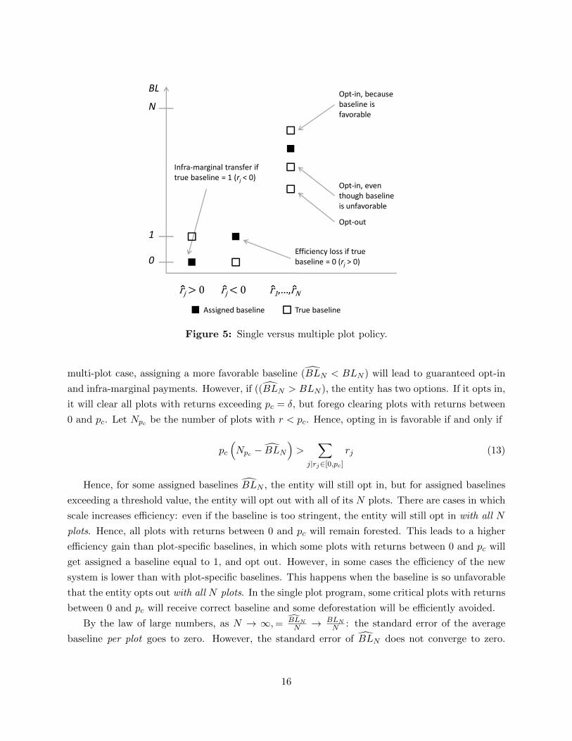
Figure 5
BL
1
0Efficiency loss if true
baseline = 0 (rj > 0)
Infra-marginal transfer if
true baseline = 1 (rj < 0)
N
Assigned baseline True baseline
Opt-out
Opt-in, even
though baseline
is unfavorable
Opt-in, because
baseline is
favorable
rj > 0 rj < 0 r1,…,rN
Figure 5: Single versus multiple plot policy.
multi-plot case, assigning a more favorable baseline (B̂LN < BLN ) will lead to guaranteed opt-in
and infra-marginal payments. However, if ((B̂LN > BLN ), the entity has two options. If it opts in,
it will clear all plots with returns exceeding pc = δ, but forego clearing plots with returns between
0 and pc. Let Npc be the number of plots with r < pc. Hence, opting in is favorable if and only if
pc
(Npc − B̂LN
)>
∑j|rj∈[0,pc]
rj (13)
Hence, for some assigned baselines B̂LN , the entity will still opt in, but for assigned baselines
exceeding a threshold value, the entity will opt out with all of its N plots. There are cases in which
scale increases efficiency: even if the baseline is too stringent, the entity will still opt in with all N
plots. Hence, all plots with returns between 0 and pc will remain forested. This leads to a higher
efficiency gain than plot-specific baselines, in which some plots with returns between 0 and pc will
get assigned a baseline equal to 1, and opt out. However, in some cases the efficiency of the new
system is lower than with plot-specific baselines. This happens when the baseline is so unfavorable
that the entity opts out with all N plots. In the single plot program, some critical plots with returns
between 0 and pc will receive correct baseline and some deforestation will be efficiently avoided.
By the law of large numbers, as N → ∞,= B̂LNN → BLN
N : the standard error of the average
baseline per plot goes to zero. However, the standard error of B̂LN does not converge to zero.
16
Therefore, it is possible that the entity gets assigned a baseline that it so unfavorable that it
decides to opt out with all N plots. Since this standard error only grows at rate√n while the
expected benefit from program participation grows at rate n, the probability of opt-in approaches
1 as N →∞ and the efficient solution will be obtained.
In the limit, larger scale will lead to the same efficient outcome as under the full information
voluntary program. However, real-world programs can only be scaled up to a finite number of
plots.20 We therefore explore the effects of moderate increases in scale numerically in the next
section.
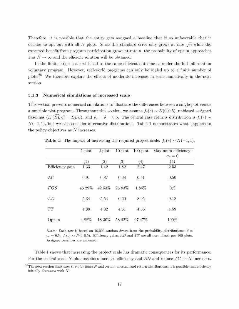
3.1.3 Numerical simulations of increased scale
This section presents numerical simulations to illustrate the differences between a single-plot versus
a multiple plot program. Throughout this section, we assume fε(ε) ∼ N(0, 0.5), unbiased assigned
baselines (E[(B̂LN ] = BLN ), and pc = δ = 0.5. The central case returns distribution is fr(r) ∼N(−1, 1), but we also consider alternative distributions. Table 1 demonstrates what happens to
the policy objectives as N increases.
Table 1: The impact of increasing the required project scale: fr(r) ∼ N(−1, 1).
1-plot 2-plot 10-plot 100-plot Maximum efficiency:σε = 0
(1) (2) (3) (4) (5)
Efficiency gain 1.33 1.42 1.82 2.47 2.53
AC 0.91 0.87 0.68 0.51 0.50
FOS 45.29% 42.53% 26.83% 1.86% 0%
AD 5.34 5.54 6.60 8.95 9.18
TT 4.88 4.82 4.51 4.56 4.59
Opt-in 4.88% 18.30% 58.42% 97.47% 100%
Notes: Each row is based on 10,000 random draws from the probability distributions. δ =
pc = 0.5. fε(ε) ∼ N(0, 0.5). Efficiency gains, AD and TT are all normalized per 100 plots.
Assigned baselines are unbiased.
Table 1 shows that increasing the project scale has dramatic consequences for its performance.
For the central case, N -plot baselines increase efficiency and AD and reduce AC as N increases.
20The next section illustrates that, for finite N and certain unusual land return distributions, it is possible that efficiencyinitially decreases with N .
17
100 plots are enough to approach the efficient solution. The reason is that the observation error nor-
malized per plot decreases as N grows, and the probability of opt-in becomes very high (97.47%).21
This high opt-in rate signals efficiency though Table 1 shows that most gains are achieved through
the first 5% of plots that participate. Hence, scale mitigates adverse selection for the central case
returns distribution.
The central case returns distribution reflects that in most developing countries, the majority
of the forested land is not at threat of deforestation, at least in the short to medium run. Still,
we test the robustness of the result by analyzing the effects of project scale for two other return
distributions: a N(0, 1) distribution (which implies that 50% of the forest will be cleared absent
any policy) and a symmetric bimodal normal BMN(0.5, 0.1) distribution with modes at -0.5 and
0.5 and standard deviation σr = 0.1. The latter distribution is unlikely to represent reality, but
illustrates that - for finite N - efficiency does not monotonically increase in N .
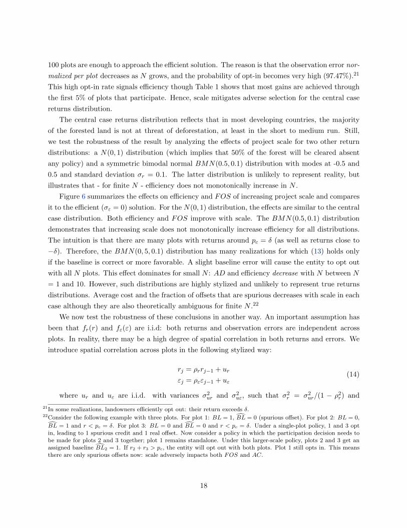
Figure 6 summarizes the effects on efficiency and FOS of increasing project scale and compares
it to the efficient (σε = 0) solution. For the N(0, 1) distribution, the effects are similar to the central
case distribution. Both efficiency and FOS improve with scale. The BMN(0.5, 0.1) distribution
demonstrates that increasing scale does not monotonically increase efficiency for all distributions.
The intuition is that there are many plots with returns around pc = δ (as well as returns close to
−δ). Therefore, the BMN(0, 5, 0.1) distribution has many realizations for which (13) holds only
if the baseline is correct or more favorable. A slight baseline error will cause the entity to opt out
with all N plots. This effect dominates for small N : AD and efficiency decrease with N between N
= 1 and 10. However, such distributions are highly stylized and unlikely to represent true returns
distributions. Average cost and the fraction of offsets that are spurious decreases with scale in each
case although they are also theoretically ambiguous for finite N .22
We now test the robustness of these conclusions in another way. An important assumption has
been that fr(r) and fε(ε) are i.i.d: both returns and observation errors are independent across
plots. In reality, there may be a high degree of spatial correlation in both returns and errors. We
introduce spatial correlation across plots in the following stylized way:
rj = ρrrj−1 + ur
εj = ρεεj−1 + uε(14)
where ur and uε are i.i.d. with variances σ2ur and σ2
uε, such that σ2r = σ2
ur/(1 − ρ2r) and
21In some realizations, landowners efficiently opt out: their return exceeds δ.22Consider the following example with three plots. For plot 1: BL = 1, B̂L = 0 (spurious offset). For plot 2: BL = 0,
B̂L = 1 and r < pc = δ. For plot 3: BL = 0 and B̂L = 0 and r < pc = δ. Under a single-plot policy, 1 and 3 optin, leading to 1 spurious credit and 1 real offset. Now consider a policy in which the participation decision needs tobe made for plots 2 and 3 together; plot 1 remains standalone. Under this larger-scale policy, plots 2 and 3 get anassigned baseline B̂L2 = 1. If r2 + r3 > pc, the entity will opt out with both plots. Plot 1 still opts in. This meansthere are only spurious offsets now: scale adversely impacts both FOS and AC.
18
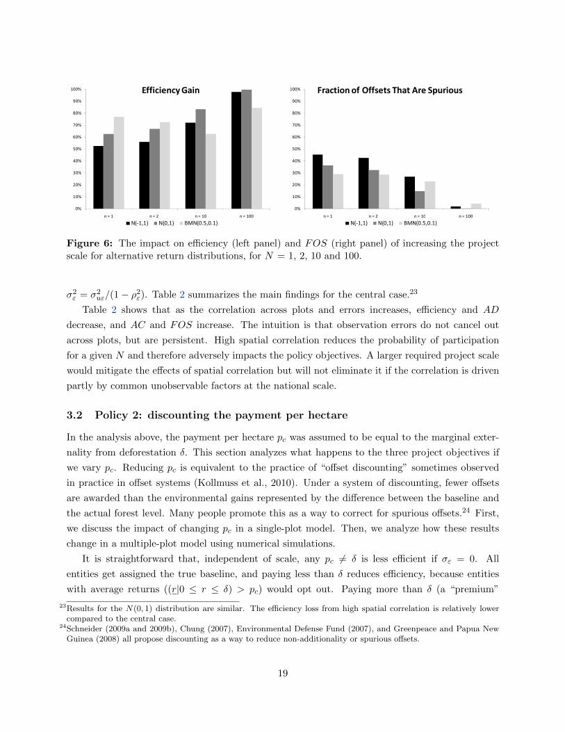
Figure 6
0%
10%
20%
30%
40%
50%
60%
70%
80%
90%
100%
n = 1 n = 2 n = 10 n = 100
Efficiency Gain
N(-1,1) N(0,1) BMN(0.5,0.1)
0%
10%
20%
30%
40%
50%
60%
70%
80%
90%
100%
n = 1 n = 2 n = 10 n = 100
Fraction of Offsets That Are Spurious
N(-1,1) N(0,1) BMN(0.5,0.1)
Figure 6: The impact on efficiency (left panel) and FOS (right panel) of increasing the projectscale for alternative return distributions, for N = 1, 2, 10 and 100.
σ2ε = σ2
uε/(1− ρ2ε). Table 2 summarizes the main findings for the central case.23
Table 2 shows that as the correlation across plots and errors increases, efficiency and AD
decrease, and AC and FOS increase. The intuition is that observation errors do not cancel out
across plots, but are persistent. High spatial correlation reduces the probability of participation
for a given N and therefore adversely impacts the policy objectives. A larger required project scale
would mitigate the effects of spatial correlation but will not eliminate it if the correlation is driven
partly by common unobservable factors at the national scale.
3.2 Policy 2: discounting the payment per hectare
In the analysis above, the payment per hectare pc was assumed to be equal to the marginal exter-
nality from deforestation δ. This section analyzes what happens to the three project objectives if
we vary pc. Reducing pc is equivalent to the practice of “offset discounting” sometimes observed
in practice in offset systems (Kollmuss et al., 2010). Under a system of discounting, fewer offsets
are awarded than the environmental gains represented by the difference between the baseline and
the actual forest level. Many people promote this as a way to correct for spurious offsets.24 First,
we discuss the impact of changing pc in a single-plot model. Then, we analyze how these results
change in a multiple-plot model using numerical simulations.
It is straightforward that, independent of scale, any pc 6= δ is less efficient if σε = 0. All
entities get assigned the true baseline, and paying less than δ reduces efficiency, because entities
with average returns ((r|0 ≤ r ≤ δ) > pc) would opt out. Paying more than δ (a “premium”
23Results for the N(0, 1) distribution are similar. The efficiency loss from high spatial correlation is relatively lowercompared to the central case.
24Schneider (2009a and 2009b), Chung (2007), Environmental Defense Fund (2007), and Greenpeace and Papua NewGuinea (2008) all propose discounting as a way to reduce non-additionality or spurious offsets.
19
Table 2: The impact of spatially correlated returns and observation errors: N = 1 and N = 100.fr(r) ∼ N(−1, 1).
1-plot 100-plot 100-plot 100-plot 100-plot σε = 0ρr = ρε = 0 ρr = ρε = 0.5 ρr = ρε = 0.9 ρr = ρε = 0.99
(1) (2) (3) (4) (5) (6)
Efficiency gain 1.33 2.47 2.41 2.02 1.59 2.53
AC 0.91 0.51 0.52 0.61 0.80 0.50
FOS 45.29% 1.86% 3.54% 17.76% 37.69% 0%
AD 5.34 8.95 8.72 7.27 5.72 9.18
TT 4.88 4.56 4.52 4.42 4.59 4.59
Opt-in 4.88% 97.47% 94.96% 78.40% 37.28% 100%
Notes: Each row is based on 10,000 random draws from the probability distributions δ = pc = 0.5. fε(ε) ∼ N(0, 0.5).
Efficiency gains, AD and TT are all normalized per 100 plots. Assigned baselines are unbiased.
rather than a “discount”) reduces efficiency because some entities will opt in even though their
private gains from deforestation exceed the full environmental cost. This is inefficient from an
economic perspective. In the single-plot model with full and symmetric information, the change
in efficiency relative to a no policy case was given in (1). A simple application of Leibniz’ Rule
yields that efficiency is maximized when pc = δ. We will now investigate if this result changes with
asymmetric information - i.e. when σε > 0.
3.2.1 Discounting in the single-plot model
In the single-plot model, the introduction of observation error does not change the conclusion that
the most efficient payment is pc = δ. The efficiency change relative to no policy equals
∆S (pc) =
pc∫0
(δ − r)
∞∫−r
fε (ε) dε
fr (r) dr (15)
Proposition 2. In the single-plot model, efficiency is maximized for pc = δ, regardless of fε(ε).
Proof. The first order condition is given by d(∆S(pc))dpc
= (δ − pc)
(∞∫−pc
fε (ε) dε
)fr (pc), using
Leibniz’ Rule. Since∞∫−pc
fε (ε) dε > 0 for any fε(ε) and fr(pc) ≥ 0, efficiency is maximized when
pc = δ.
20
We now investigate what happens to the other policy objectives as the payment pc varies.
Proposition 3. AD, MT , IT , and TT are globally (weakly) increasing in pc; FOS is globally
(weakly) decreasing in pc.
Proof. AD =pc∫0
(∞∫−rfε (ε) dε
)fr (r) dr. The derivative of AD w.r.t. pc is
(∞∫−pc
fε (ε) dε
)fr (pc)
≥ 0 ∀pc, proving the first statement. The derivative of MT (first term in (9)) w.r.t. pc ispc∫0
(∞∫−rfε (ε) dε
)fr (r) dr + pc
(∞∫−pc
fε (ε) dε
)fr (pc) ≥ 0 ∀pc. The derivative of IT (second term
in (9)) w.r.t. pc is0∫−∞
(∞∫−rfε (ε) dε
)fr (r) dr ≥ 0 ∀pc. Hence, the derivative of TT w.r.t. pc
is weakly greater than zero ∀pc. Finally, using (9), FOS = IT/TT =0∫−∞
(∞∫−rfε (ε) dε
)fr (r) dr/
pc∫−∞
(∞∫−rfε (ε) dε
)fr (r) dr. Since the denominator is monotonically (weakly) increasing in pc, FOS
is monotonically (weakly) decreasing in pc.
Proposition 3 demonstrates that, contrary to the intended effect, the fraction of offsets that is
spurious, FOS, increases when the offset price is discounted (i.e., reduced): as pc falls the share of
offsets that is spurious rises toward 1.
The effect of changing pc on AC is ambiguous. Since AD is bounded, very high values of pc
will lead to increasing AC. For intermediate values of pc, a small increase in pc can either lead to
almost no additional deforestation, or a large increase in avoided deforestation, depending on the
specification of the return distribution fr(r). For instance, if fr(r) = 0 for r ∈ [0, p], then AC will
be infinite for pc ≤ p and achieve a global minimum for some pc > p. Hence, AC can either be
increasing or decreasing in pc.
We conclude that, in the single-plot model, efficiency is maximized by paying pc = δ. Paying
more reduces FOS, leads to more AD, but requires higher transfers. The effect on AC is ambiguous
for low values of pc, but eventually AC must increase.
3.2.2 Discounting in the multi-plot model
In the multi-plot model, pc = δ no longer unambiguously maximizes efficiency. The intuition is
as follows. Raising pc above δ has two countervailing effects on efficiency. First, it will increase
the opt-in probability. This increases efficiency because it helps prevent deforestation of plots with
returns below δ. Second, it causes certain forest to be inefficiently prevented from deforestation.
The relative strength of these channels determines whether a higher pc can be more efficient than
pc = δ. A lower pc will never increase efficiency, since it will both reduce opt-in and cause inefficient
21
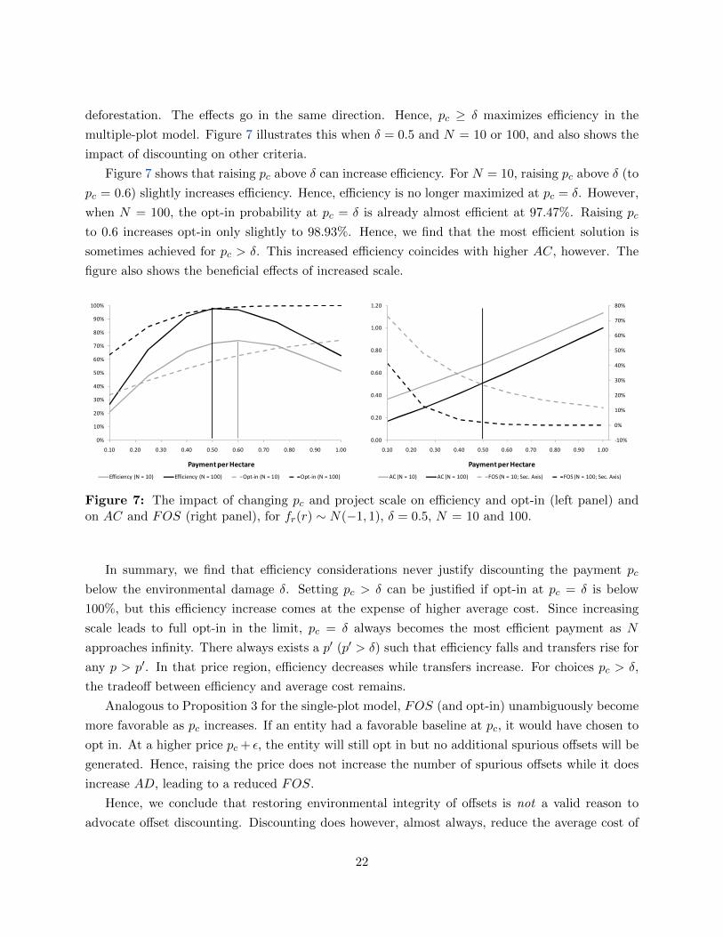
deforestation. The effects go in the same direction. Hence, pc ≥ δ maximizes efficiency in the
multiple-plot model. Figure 7 illustrates this when δ = 0.5 and N = 10 or 100, and also shows the
impact of discounting on other criteria.
Figure 7 shows that raising pc above δ can increase efficiency. For N = 10, raising pc above δ (to
pc = 0.6) slightly increases efficiency. Hence, efficiency is no longer maximized at pc = δ. However,
when N = 100, the opt-in probability at pc = δ is already almost efficient at 97.47%. Raising pc
to 0.6 increases opt-in only slightly to 98.93%. Hence, we find that the most efficient solution is
sometimes achieved for pc > δ. This increased efficiency coincides with higher AC, however. The
figure also shows the beneficial effects of increased scale.Figure 7
0%
10%
20%
30%
40%
50%
60%
70%
80%
90%
100%
0.10 0.20 0.30 0.40 0.50 0.60 0.70 0.80 0.90 1.00
Payment per Hectare
Efficiency (N = 10) Efficiency (N = 100) Opt-in (N = 10) Opt-in (N = 100)
-10%
0%
10%
20%
30%
40%
50%
60%
70%
80%
0.00
0.20
0.40
0.60
0.80
1.00
1.20
0.10 0.20 0.30 0.40 0.50 0.60 0.70 0.80 0.90 1.00
Payment per Hectare
AC (N = 10) AC (N = 100) FOS (N = 10; Sec. Axis) FOS (N = 100; Sec. Axis)
Figure 7: The impact of changing pc and project scale on efficiency and opt-in (left panel) andon AC and FOS (right panel), for fr(r) ∼ N(−1, 1), δ = 0.5, N = 10 and 100.
In summary, we find that efficiency considerations never justify discounting the payment pc
below the environmental damage δ. Setting pc > δ can be justified if opt-in at pc = δ is below
100%, but this efficiency increase comes at the expense of higher average cost. Since increasing
scale leads to full opt-in in the limit, pc = δ always becomes the most efficient payment as N
approaches infinity. There always exists a p′ (p′ > δ) such that efficiency falls and transfers rise for
any p > p′. In that price region, efficiency decreases while transfers increase. For choices pc > δ,
the tradeoff between efficiency and average cost remains.
Analogous to Proposition 3 for the single-plot model, FOS (and opt-in) unambiguously become
more favorable as pc increases. If an entity had a favorable baseline at pc, it would have chosen to
opt in. At a higher price pc + ε, the entity will still opt in but no additional spurious offsets will be
generated. Hence, raising the price does not increase the number of spurious offsets while it does
increase AD, leading to a reduced FOS.
Hence, we conclude that restoring environmental integrity of offsets is not a valid reason to
advocate offset discounting. Discounting does however, almost always, reduce the average cost of
22
offsets. If the discounted price is achieved by limiting demand (e.g., limiting the number of offsets
that can enter the market), so that buyers pay less than the market price for a unit that is then
fully fungible with other units (i.e., a 1:1 trading ratio without downward adjustment of the cap,
as is the case in the Clean Development Mechanism), buyers will reap gains and the environmental
outcome will be negative. If however the gains to industrialized countries are spent on additional
mitigation (as it is with (t : 1, t > 1) trading ratios) this could have a positive environmental effect
even if the cap is not adjusted.25 This might however be more efficiently achieved through changes
in baselines.
3.3 Policy 3: changing the generosity of the assigned baseline
Another policy choice for the regulator is to set a baseline that is, in expectation, too high or too
low. In other words, the government assigns the following baselines for plot i
B̂Li =
{1 if r̂i ≤ r∗
0 if r̂i > r∗
}(16)
where r∗ is a specified return set by the government. The government, aware of adverse selection,
may try to pay only landowners who are most likely to deforest in the baseline, for instance by
choosing pc > r∗ > 0. Assuming pc = δ, we analyze the impact of this policy change on the
various criteria: efficiency, AD, AC and FOS. To provide intuition, we first discuss the impact in
the context of the single-plot model. Then, we present numerical simulations of the multiple-plot
model.
3.3.1 Changing baselines in the single-plot model
Proposition 4. More generous baselines (weakly) increase efficiency and AD, but require a (weakly)
higher TT .
Proof. The efficiency change relative to no policy equals ∆S (r∗) =pc∫0
(pc − r)
(∞∫
r∗−rfε (ε) dε
)fr (r) dr. By Leibniz’ Rule, this expression is globally weakly decreasing in r∗. Hence, effi-
ciency is maximized if r∗ → −∞. AD is given by AD(r∗) = Pr(0 ≤ r ≤ pc, r̂ > r∗) =pc∫0
(∞∫
r∗−rfε (ε) dε
)fr (r) dr, which is globally weakly decreasing in r∗. TT is given by TT (r∗) =
pcpc∫−∞
(∞∫
r∗−rfε (ε) dε
)fr (r) dr, which is also globally weakly decreasing in r∗.
25Note that, if trading ratios are used without adjusting the cap, the environmental effect could be negative evenfor large t. A straightforward example is a returns distribution with positive probability mass below zero, but noprobability mass between 0 and pc.
23
The effect on FOS is theoretically ambiguous and depends on the baseline error distribution.
Using (9) and (10), FOS = OS/AD = IT/TT is decreasing in r∗ if and only if MT/IT is in-
creasing in r∗. We can write MT/IT =pc∫0
(∞∫
r∗−rfε (ε) dε
)fr (r) dr/
0∫−∞
(∞∫
r∗−rfε (ε) dε
)fr (r) dr =
pc∫0
(1− Fε(r∗ − r)) fr (r) dr/0∫−∞
(1− Fε(r∗ − r)) fr (r) dr. If this expression is increasing in r∗, FOS
is decreasing in baseline stringency. This condition will certainly hold if the baseline error is bounded
from above.
The fact that efficiency increases as the baseline becomes more generous is not surprising, since
in the limit this is equivalent to assigning a no-forest baseline or a subsidy of pc per hectare of
forest standing. As discussed in Section 2, such a subsidy is indeed efficient but requires a large
infra-marginal transfer.
Using (10) and making OS and AD functions of r∗ we can see that the effect of r∗ on AC is
also ambiguous. OS, the amount of spurious offsets, is decreasing in r∗, but so is AD. The shape
of AC is dependent on the return distribution fr(r).
Numerical illustration
Figure 8
-40%
-20%
0%
20%
40%
60%
80%
100%
0.00
0.50
1.00
1.50
2.00
2.50
3.00
3.50
4.00
4.50
-1.00 -0.75 -0.50 -0.25 0.00 0.25 0.50 0.75 1.00
Required Return (r*)
AC AD per 10 Hectares Efficiency Gain (Sec. Axis) FOS (Sec. Axis)
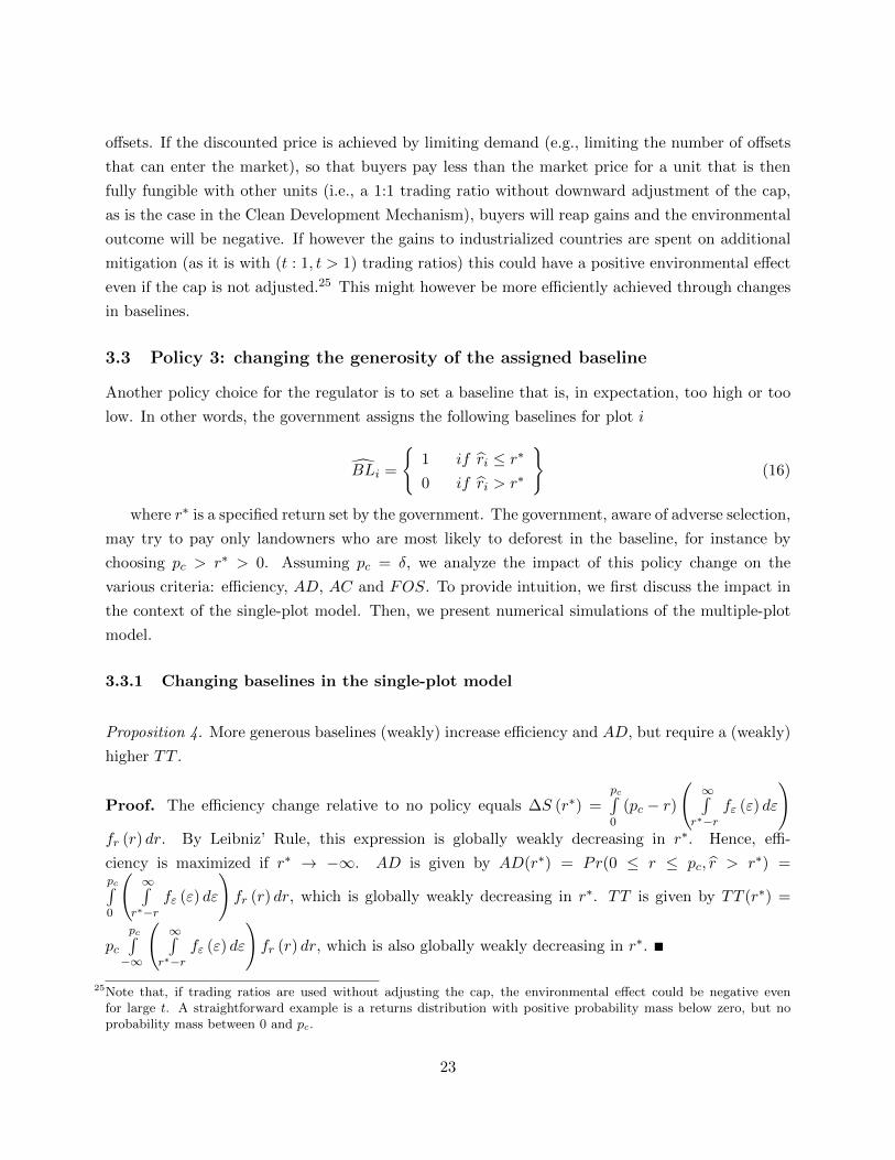
Figure 8: The impact of baseline generosity on the project objectives for the central case.
Figure 8 shows that for reasonable returns distributions like our central case, FOS and AC
are both decreasing in r∗ (as baselines become more stringent). For very stringent baselines FOS
24
becomes negative: the environmental gains are greater than the number of traded offsets. Efficiency,
lower average cost and offset quality are conflicting policy aims for this policy option also: efficiency
requires setting r∗ low (generous baseline), while minimizing average cost and maximizing offset
quality requires setting r∗ high (stringent baseline).
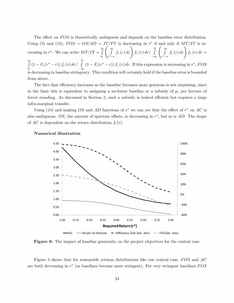
3.3.2 Changing baselines in the multiple-plot model
The conclusions from the single-plot model also hold in the multiple-plot model. Figure 9 illustrates
the effect of assigning baselines that are too (un)favorable in expectation for the central case returns
distribution. The true baseline equals 84 (84 out of 100 plots will remain forested in absence of a
policy). The figure shows that increasing the baseline (i.e., making it less favorable) unambiguously
reduces efficiency and AD, but also reduces AC and FOS.Figure 9
-150%
-100%
-50%
0%
50%
100%
0.00
0.10
0.20
0.30
0.40
0.50
0.60
0.70
0.80
0.90
1.00
78 81 84 87 90 93
Assigned Baseline
AC AD per Hectare Efficiency Gain (Sec. Axis) FOS (Sec. Axis)
Figure 9: The impact of changing baseline generosity on the project objectives, for fr(r) ∼N(−1, 1) and N = 100. 84 is an unbiased baseline.
This section has shown that only increasing project scale improves all objectives simultaneously
(for “typical” returns distributions). Discounting offsets and changing baseline generosity affect
the objectives in opposing directions. Discounting offsets reduces efficiency, AD and offset quality,
but improves the value for money for funders. Making assigned baselines more stringent reduces
efficiency and AD, but improves quality and value. This illustrates the conflicting nature of these
25
policy objectives. It also illustrates that tightening the baseline should be favored over offset
discounting if environmental integrity of offsets is a key policy concern and not enough of the
gains to industrialized countries from discounting are spent on additional mitigation (e.g. through
trading ratios and/or reducing the cap) to counteract the fall in offset quality.
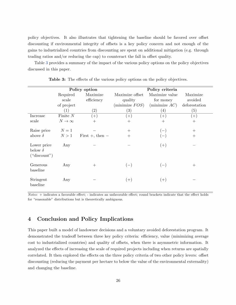
Table 3 provides a summary of the impact of the various policy options on the policy objectives
discussed in this paper.
Table 3: The effects of the various policy options on the policy objectives.
Policy option Policy criteriaRequired Maximize Maximize offset Maximize value Maximize
scale efficiency quality for money avoidedof project (minimize FOS) (minimize AC) deforestation
(1) (2) (3) (4) (5)
Increase Finite N (+) (+) (+) (+)scale N →∞ + + + +
Raise price N = 1 − + (−) +above δ N > 1 First +, then − + (−) +
Lower price Any − − (+) −below δ(“discount”)
Generous Any + (−) (−) +baseline
Stringent Any − (+) (+) −baseline
Notes: + indicates a favorable effect; - indicates an unfavorable effect; round brackets indicate that the effect holds
for “reasonable” distributions but is theoretically ambiguous.
4 Conclusion and Policy Implications
This paper built a model of landowner decisions and a voluntary avoided deforestation program. It
demonstrated the tradeoff between three key policy criteria: efficiency, value (minimizing average
cost to industrialized countries) and quality of offsets, when there is asymmetric information. It
analyzed the effects of increasing the scale of required projects including when returns are spatially
correlated. It then explored the effects on the three policy criteria of two other policy levers: offset
discounting (reducing the payment per hectare to below the value of the environmental externality)
and changing the baseline.
26
We have four main findings. First, under almost all circumstances, voluntary deforestation
programs (or, in fact, general offset programs) will perform better with increased required scale of
project. Second, offset discounting and setting more stringent baselines highlight the tradeoffs in-
volved in policy design: efficient policy may involve high transfers that make the policy unattractive
to the industrialized countries which will fund them. Both policies reduce efficiency but generally
raise value. Moreover, there is still an efficiency gain relative to no policy. Third, discounting lowers
the quality of offsets and does not improve the environmental outcome, at least if not accompanied
by a sufficiently high trading ratio. In some cases, even a high trading ratio leads to a worse en-
vironmental outcome. Therefore, the main rationale for offset discounting is to raise the value of
the policy to industrialized countries. Fourth, making baselines more stringent does increase the
quality of offsets.
Our key messages for policy makers are three. First, make ’projects’ as large as possible.
Regional or national scale programs where funds or offsets are transferred to the government on
the basis of aggregated regional or national monitoring data will be much more efficient and offer
better value for money. Although baseline deforestation rates are still difficult to predict at the
national or regional scale, the errors fall dramatically relative to small scale prediction.
Second, recognize that the primary purpose of offset discounting or below market prices is to
reduce the cost to industrialized countries so that paying for avoided deforestation becomes an
attractive mitigation option for them. It actually increases the share of funds that go to spurious
offsets and reduces efficiency. Discounting can only be justified on environmental integrity grounds
if the trading ratio with “regular” cap-and-trade credits compensates for the loss of offset quality. In
that case, discounting can extract rents from sellers to pay for additional environmental protection.
The use of baselines more stringent than business as usual typically does reduce the number and
fraction of spurious offsets while simultaneously reducing the cost to industrialized countries, but
reduces efficiency.
Third, invest in research to improve understanding of local and global deforestation drivers. This
will allow more accurate assessment of returns distributions and their evolution and hence more
accurate prediction of baseline deforestation. Moreover, this will help identify domestic policies to
effectively control deforestation.
This paper has highlighted the tradeoffs involved in various policy design options for avoiding
deforestation. In future work, we will present a framework in which industrialized and forest-
covered developing countries can explore these trade-offs, subject to the restriction that the policy
has to be individually rational for both parties. By defining the Pareto efficient bargaining set we
can explore its determinants and give guidance to policy makers who may seek to expand the set
and to negotiators who want to find agreements within the set (and in their countries’ favor).
If countries can be encouraged to be more generous, by pushing less to lower the average cost
of (real) offsets or by accepting more stringent baselines, it will be easier to create an efficient
27
international framework to avoid deforestation. Combined with effective domestic policies that
respond to the international incentives, this could meet the expectations of those who promote
avoided deforestation as a key climate mitigation option in the short term.
References
• Andam, K., P. Ferraro, A. Pfaff, J. Robalino, and A. Sanchez. 2008. “Measuring the Effectivenessof Protected-Area Networks in Reducing Deforestation.” Proceedings of the National Academyof Sciences 105(42): 16089-16094.
• Angelsen, A. 2010. “Policies for reduced deforestation and their impact on agricultural pro-duction”, in Climate Mitigation and Agricultural Productivity in Tropical Landscapes, SpecialFeature, Proceedings of the National Academy of Sciences. Accessed online on 19 July 2010.
• Angelsen, A. (ed.). 2008. “Moving ahead with REDD: Issues, options and implications.” CIFOR,Bogor, Indonesia.
• Arguedas, C. and D.P. van Soest. 2009. “On reducing the windfall profits in environmentalsubsidy programs.” Journal of Environmental Economics and Management 58(2): 192-205.
• Busch J., B. Strassburg, A. Cattaneo, R. Lubowski, A. Bruner, R. Rice, A. Creed, R. Ashton, andF. Boltz. 2009. “Comparing climate and cost impacts of reference levels for reducing emissionsfrom deforestation.” Environmental Research Letters 4(4).
• Chomitz, K. 2007. “At Loggerheads? Agricultural Expansion, Poverty Reduction, and Environ-ment in the Tropics.” World Bank: Washington, DC.
• Environmental Defense Fund. 2007. “CDM and the Post-2012 Framework.” Discussion Paper,Vienna, August 27-31, AWG/Dialogue.
• Fischer, C. 2005. “Project-based mechanisms for emissions reductions: balancing trade-offs withbaselines.” Energy Policy 33(14): 1807-1823.
• Government of the Kingdom of Norway and Government of the Republic of Indonesia. 2010.Letter of Intent on “Cooperation on reducing greenhouse gas emissions from deforestation andforest degradation.”
• Greenpeace and Papua New Guinea. 2008. REDD proposals submitted to the United Nations.Available at http://unfccc.int.
• He, G. and R. Morse. 2010. “Making Carbon Offsets Work in the Developing World: Lessonsfrom the Chinese Wind Controversy.” Stanford University, Program on Energy and SustainableDevelopment Working Paper 90.
• Kerr, S. 1995. “Adverse Selection and Participation in International Environmental Agreements”,in Contracts and Tradeable Permit Markets in International and Domestic Environmental Pro-tection, Ph.D. Thesis, Harvard University.
28

• Kerr, S., A.S.P. Pfaff, and A. Sanchez. 2002. “The dynamics of deforestation: evidence fromCosta Rica.” Motu Manuscript. Available at http://www.motu.org.nz/files/docs/MEL0270.pdf.
• Kerr, S., J. Hendy, S. Liu and A.S.P. Pfaff. 2004. “Tropical forest protection, uncertainty andthe environmental integrity of carbon mitigation policies.” Motu Working Paper 04-03.
• Kindermann, G.E., M. Obersteiner, E. Rametsteiner, and I. McCallum. 2006. “Predicting thedeforestation trend under different carbon prices.” Carbon Balance Management 1(15).
• Kindermann, G.E., M. Obersteiner, B. Sohngen, J. Sathaye, K. Andrasko, E. Rametsteiner, B.Schlamadinger, S. Wunder, and R. Beach. 2008. “Global Cost Estimates of Reducing CarbonEmissions Through Avoided Deforestation.” Proceedings of the National Academy of Sciences105(30): 10302-10307.
• Kollmuss, A., M. Lazarus, and G. Smith. 2010. “Discounting Offsets: Issues and Options.”Stockholm Environment Institute Working Paper WP-US-1005.
• Mason, C.F. and A.J. Plantinga. 2010. “The Additionality Problem with Offsets: Optimal Con-tracts for Carbon Sequestration in Forests.” Working paper. Available at http://idei.fr/doc/conf/ere/papers 2010/paper Mason.pdf.
• Melillo, J.M., J.M. Reilly, D.W. Kicklighter, A.C. Gurgel, T.W. Cronin, S. Paltsev, B.S. Felzer,X. Wang, A.P. Sokolov, and C.A. Schlosser. 2009. “Indirect Emissions from Biofuels: HowImportant?” Science 326: 1397-1399.
• Millard-Ball, A. 2010. “Adverse Selection in an Opt-In Emissions Trading Program: The caseof sectoral no-lose targets for transportation.” Stanford University, Program on Energy andSustainable Development Working Paper 97.
• Montero, J.P. 1999. “Voluntary Compliance with Market-Based Environmental Policy: Evidencefrom the U. S. Acid Rain Program.” Journal of Political Economy 107(5): 998-1033.
• Montero, J.P. 2000. “Optimal design of a phase-in emissions trading program.” Journal of PublicEconomics 75(2): 273-291.
• Pfaff, A., S. Kerr, L. Lipper, R. Cavatassi, B. Davis, J. Hendy, A. Sanchez-Azofeifa. 2007. “Willbuying tropical forest carbon benefit the poor? Evidence from Costa Rica.” Land Use Policy24(3): 600-610.
• Plantinga, A.J. and K.R. Richards. 2008. “International Forest Carbon Sequestration in aPost-Kyoto Agreement.” Discussion Paper 08-11, Harvard Project on International ClimateAgreements, Belfer Center for Science and International Affairs, Harvard Kennedy School.
• Robalino, J., A. Pfaff, G. A. Sanchez-Azofeifa, F. Alpizar, C. Leon, and C. M. Rodriguez. 2008.“Deforestation Impacts of Environmental Services Payments: Costa Rica’s PSA Program 2000-2005.” Environment for Development Discussion Paper 08-24. Washington, DC: Resources forthe Future.
• Sanchez-Azofeifa, A., A. Pfaff, J.A. Robalino, and J.P. Boomhower. 2007. “Costa Rica’s Paymentfor Environmental Services Program: Intention, Implementation, and Impact.” ConservationBiology 21(5): 1165-1173.
29
• Sathaye J., W. Makundi, L. Dale, P. Chan, and K. Andrasko. 2006. “GHG mitigation potential,costs, and benefits in global forests.” Energy Journal 27(3): 127-162.
• Schneider, L. 2009a. “Assessing the additionality of CDM projects: practical experiences andlessons learned.” Climate Policy 9(3): 242-254
• Schneider, L. 2009b. “A Clean Development Mechanism with global atmospheric benefits fora post-2012 climate regime.” International Environmental Agreements: Politics, Law and Eco-nomics 9(2): 95-111.
• Stern, N. 2006. The economics of climate change: The Stern Review. Cambridge UniversityPress: Cambridge, MA.
• Strand, J. 2010. “Carbon Offsets with Endogenous Environmental Policy”. World Bank PolicyResearch Working Paper 5296.
• Wara, M. and D. Victor. 2008. “A realistic policy on international carbon offsets.” StanfordUniversity, Program on Energy and Sustainable Development Working Paper 74.
• Wise, M., K. Calvin, A. Thomson, L. Clarke, B. Bond-Lamberty, R. Sands, S.J. Smith, A.Janetos, and J. Edmonds. 2009. “Implications of Limiting CO2 Concentrations for Land Useand Energy.” Science 324: 1183-1186.
30