Big G∗

Lydia Cox†, Gernot J. Muller‡, Ernesto Pasten§,Raphael Schoenle¶, and Michael Weber‖

June 14, 2021

Abstract

“Big G” typically refers to aggregate government spending on a homogeneous good. In thispaper, we open up this construct by analyzing the entire universe of procurement contracts ofthe U.S. federal government and establish five facts. First, government spending is granular;that is, it is concentrated in relatively few firms and sectors. Second, relative to privatespending its composition is biased. Third, at the contract, firm and sectoral level moderatepersistence characterizes spending. Fourth, idiosyncratic variation dominates fluctuationsin spending. Last, government spending is concentrated in sectors with relatively stickyprices. Accounting for these facts within a stylized New Keynesian model offers new insightsinto the fiscal transmission mechanism and aligns the model predictions with the empiricalevidence: Fiscal shocks hardly impact inflation, little crowding out of private expenditureoccurs, markups can be either pro-cyclical or counter-cyclical, and the multiplier tends to belarger compared to a one-sector benchmark.

Keywords: Government spending, federal procurement, granularity, sectoral heterogeneity,fiscal policy transmission, monetary policy

JEL Classification: E62, E32

∗We acknowledge outstanding research assistance by Jiacheng Feng. We thank Klaus Adam, Regis Barnichon,Christian Bayer, Benjamin Born, Gabriel Chodorow-Reich, Zeno Enders, Emmanuel Farhi, Xavier Gabaix, YuriyGorodnichenko, Edward Knotek, Valerie Ramey, Ludwig Straub and conference and seminar participants at theBanco Central de Chile Heterogeneity in Macroeconomics Conference, Federal Reserve Banks of Boston andCleveland, the NBER Monetary Economics Meeting, PUC Santiago, the University of Tuebingen, and the VfSMonetary Meeting Frankfurt for valuable comments. Weber also thanks the Fama-Miller Center and the FamaResearch Fund at the University of Chicago Booth School of Business for financial support. Schoenle and Weberalso gratefully acknowledge support from the National Science Foundation under grant number 1756997. Theviews expressed herein are solely those of the authors and do not necessarily reflect the views of the Central Bankof Chile, the Federal Reserve Bank of Cleveland or the Federal Reserve System.

†Harvard University. e-Mail: lcox@g.harvard.edu.‡University of Tubingen and CEPR. e-Mail: gernot.mueller@uni-tuebingen.de.§Central Bank of Chile and Toulouse School of Economics. e-Mail: epasten@bcentral.cl.¶Brandeis University, Cleveland Fed, and CEPR. e-Mail: schoenle@brandeis.edu.‖Booth School of Business, University of Chicago and NBER. e-Mail: michael.weber@chicagobooth.edu.

1 Introduction

What is “Big G”? In the national accounts, G represents government spending—the part of

GDP that comprises government consumption of goods and services plus investment.1 This

convention possibly helps explain why research on fiscal policy typically entertains a somewhat

crude notion of government spending as spending on a homogeneous good, isomorphic to GDP.

In empirical and theoretical work, we frequently refer to it as G, and the literature assumes

policymakers can freely adjust it over time. The recent “renaissance of fiscal research” surveyed

by Ramey (2019) has changed little in this regard. A number of recent papers have started

to study the role of heterogeneity for the fiscal transmission mechanism but focus exclusively

on heterogeneity on the household side (McKay and Reis, 2016; Auclert et al., 2018; Hagedorn

et al., 2019).

The starting point of our paper is the observation that government spending itself is

fundamentally heterogeneous. Government spending is not simply one large transaction. It

is composed of a large number of smaller transactions whose composition differs from the other

components of aggregate demand. We first establish five facts about government spending and

then reassess the fiscal transmission mechanism through the lens of a simple two-sector New

Keynesian model, which captures all five facts in a stylized way. Allowing for heterogeneity of

government spending has first-order effects on the transmission mechanism, aligning the model

prediction with the empirical evidence.

Our empirical anatomy of government spending relies on a database that has only recently

become accessible: USASpending.gov. The database provides detailed information on the entire

universe of procurement contracts by the federal government since 2001.2 For each year, the

database records several million government procurement transactions. While the database does

not cover all components of government spending, it is unique in detail and scope: it covers 40

percent of total federal spending, and 16 percent of general government spending. The facts

1Throughout, we refer to government spending even though our data does not cover government employment.Note that government spending does not include transfer payments. For details, see Figure 1.

2Data on government contracts go back further, see https://www.archives.gov/research/

electronic-records/reference-report/federal-contracts. The data, however, largely covers defensecontracts, and the data are not as comprehensive as USASpending.gov. Earlier work uses procurement data bythe Department of Defense to estimate fiscal multipliers or the effects of government spending shocks (Fisherand Peters, 2010; Nakamura and Steinsson, 2014; Dupor and Guerrero, 2017; Demyanyk et al., 2019; Auerbachet al., 2020). Hebous and Zimmermann (2021) use the data to study the effect of federal purchases on firminvestment. The data set has also been studied in other contexts: e.g. Decarolis et al. (2020) assess the impactof bureaucratic competence on procurement outcomes. Appendix A.2 provides additional details.

1

we document hold equally for procurement contracts of the Department of Defense (DOD) and

non-DOD procurement, the latter of which has not been studied in detail due to data limitations.

Our most important facts also extend to state and local spending, which account for another

21 percent of general government spending. In contrast to the existing literature, we focus on

heterogeneity, in particular on differences in government spending across contracts, firms and

sectors; differences relative to private spending; and differences in pricing frictions. Limited

availability of micro data precludes us from extending our analysis to government employment

and wages. The existing literature guides us in the choice of the dimension of heterogeneity we

study, such as the persistence of government spending or pricing frictions.

Our first fact is that government spending is granular in the sense of Gabaix (2011): it

is concentrated among few firms and sectors. For instance, the largest ten suppliers in terms

of average annual contract value receive over a third of government contract spending and

are concentrated in a few sectors. Firms in the largest three two-digit NAICS industries are

counter-party for more than 60 percent of all government contracts. Concentration in defense

and non-defense spending is similar, and it is equally pervasive at the state and local levels.

The second fact is a sectoral bias in government spending: the allocation of government

spending across sectors differs substantially from that of private spending. For instance, the

sector with the largest share in total government spending (manufacturing) receives 30 percent

of government spending, but accounts for only 13 percent of GDP. Conversely, the sector with

the largest share in GDP (health care and social assistance) accounts for 12 percent of GDP but

less than 2 percent of government contract spending. Again, this fact holds not only for federal

spending, but also for state and local government spending.3

Third, we study the persistence of government spending because of its key role for the

fiscal transmission mechanism (Baxter and King, 1993). We find only moderate persistence

of government spending at the contract, firm, and sectoral level. The median contract has a

duration of 31 days and 90 percent of contracts last less than one year. Moreover, the turnover

of firms which are counter-party to the government is large. The median firm is in the data

3In earlier work, Ramey and Shapiro (1998) stress the sectoral bias of military buildups—World War II,the Korean War, the Vietnam War, and the Carter-Reagan buildup—as well as the 1950s construction of theU.S. highway system and the rise of federal medical spending. They then explore its implication for the fiscaltransmission in a neoclassical two-sector model. We build on their work but use more disaggregated and recentdata, and we document the bias for the universe of spending. Most importantly, we focus on variation at thebusiness-cycle frequency rather than on long swings in spending mainly due to military spending. Also, in ourtheoretical analysis, we depart from their framework and show that sectoral bias interacts with price stickiness inways which fundamentally alter the fiscal transmission mechanism.

2

for less than two years, while the firm with the median value of average annual contracts is in

the data for less than one year. At the sectoral level, we fit AR(1) processes to the data to

measure persistence and to facilitate a mapping of our data into business cycle models. The

average monthly persistence parameter is 0.42. However, in line with the political economy

of government spending, government contracts tend to spike in September.4 If we filter out

such seasonality, persistence estimates can increase substantially, up to the level that implies a

half-life of government spending processes in line with those implied by estimated VAR models.

Fourth, at business cycle frequency, idiosyncratic variation of a few influential firms and

sectors accounts for the growth of aggregate government spending. To establish this fact, we

construct the granular residual of government spending following the approach of Gabaix (2011)

and find that it explains almost 40 percent of monthly variation in aggregate government

spending growth. An alternative approach based on a decomposition of spending growth

following Foerster et al. (2011) yields similar results. While our second fact shows high

concentration of government spending in the cross-section, this fourth fact shows concentration

over time in government spending growth.

Fifth, government spending tends to be concentrated in sectors with high degrees of price

stickiness—a key modeling feature for the fiscal transmission mechanism in the New Keynesian

literature. We find that the monthly frequency of price changes in the top three two-digit

NAICS sectors that supply goods to the government is 11 percent while it is 22 percent, on

average, for the remaining sectors. In contrast, the average frequency in the top three sectors

for private consumption is 17 percent. These frequencies are estimated on the basis of the micro

data underlying the producer price index (PPI) at the Bureau of Labor Statistics (BLS), but

we document the duration of contracts in the USASpending.gov data and their pricing nature

are consistent with these estimates.

In isolation and one-by-one, these facts may not appear surprising, but so far no systematic

documentation exists. We also show that accounting for heterogeneity of government spending

in terms of our five facts has first-order effects on the fiscal transmission mechanism. To do

so, we develop a two-sector New Keynesian model with government spending. The model is

deliberately stylized in order to account for the five facts in a transparent way while minimally

departing from the conventional one-sector model (e.g. Woodford, 2011). Importantly, rather

4This seasonality suggests part of government spending is predictable. We do not pursue further quantificationbut potential anticipation of fiscal shocks has been a major theme of the empirical literature on the fiscal multiplier(Ramey, 2011; Leeper et al., 2013).

3

than postulating a driving process for G, as is commonly done, we instead model government

spending at the sectoral level—in line with fact 4.5

In our analysis, we establish a number of results, both in closed form based on limiting

cases, and quantitatively based on model simulations. We show analytically that unlike in

a one-sector model, crowding out of private expenditure can be infinite and the government

spending multiplier negative if government spending increases in a sector in which prices are

fully flexible while prices are sticky in the other sector. However, a fiscal shock in the relatively

small and sticky-price sector, toward which government spending is biased in the data (facts 1,

2 and 5), induces a fiscal multiplier that is three to four times larger than what we observe for

the one-sector benchmark. Moreover, we find the multiplier is larger the more flexible prices are

in the sector in which private spending is concentrated. Hence, it is not the overall degree of

price stickiness in the economy that determines the size of the multiplier; instead the multiplier

increases in the relative stickiness in the sector in which government spending increases. This

result is in line with the finding that the relative extent of frictions is key for aggregate dynamics

in multi-sector economies (Barsky et al., 2007, 2016; Gilchrist et al., 2017).

The intuition for these findings follows from the interaction of our heterogeneous model

features and monetary policy, which is key for the fiscal transmission mechanism in the New

Keynesian model (Woodford, 2011; Christiano et al., 2011; Farhi and Werning, 2016). In this

model, because government spending is inflationary, it induces the central bank to raise interest

rates, and private spending is crowded out due to intertemporal substitution. A number of

recent contributions show that household heterogeneity and credit frictions limit intertemporal

substitution and instead make the model more “old Keynesian” (Galı et al., 2007; McKay

et al., 2016; Kaplan et al., 2018). Sectoral bias in government spending combined with sectoral

heterogeneity in pricing frictions has a similar effect. In a nutshell, if the government spends in

relatively sticky-price sectors compared to the private sector, monetary policy needs to respond

less (via higher interest rates) to a fiscal stimulus in order to keep inflation stable. Hence,

less crowding out occurs, rendering the multiplier larger. These effects become stronger, the

larger the sectoral bias, because in this case, more private spending is concentrated in the

relatively flexible-price sector. Following a given interest rate increase, private consumption

prices fall endogenously and strongly in this sector, stabilizing overall prices and requiring a

smaller contractionary interest rate increase.

5Our empirical analysis documents several facts in more detail than what we model. These additional detailsmay provide further guidance to modelers and policymakers.

4

Importantly, such a muted impact of fiscal shocks on inflation and interest rates is also

consistent with empirical observations from fiscal VARs (Mountford and Uhlig, 2009; Corsetti

et al., 2012; Ramey, 2016). Likewise, a muted response of inflation also means the fiscal multiplier

at the zero lower bound is not much larger compared to the baseline case due to a muted real rate

response, in line with recent evidence by Ramey and Zubairy (2018). Moreover, we show that

accounting for the heterogeneity of government spending across sectors goes some way towards

accounting for the response of markups to government spending shocks for which the one-sector

model delivers counterfactual predictions (Nekarda and Ramey, 2020). In sum, once we modify

the model to account for the heterogeneity that characterizes spending data at the micro level,

the model performance also improves at the macro level.

Our paper is also related to recent work on the effect of regional fiscal policies in monetary

unions (Galı and Monacelli, 2008; Acconcia et al., 2014; Nakamura and Steinsson, 2014;

Blanchard et al., 2017; Hettig and Muller, 2018).6 In this literature, government spending is

concentrated in some spatial partition of the economy, and its composition is biased relative to

the composition of private spending. In contrast to this earlier work, we model private spending

as being determined at the sectoral level rather than at the regional level.

We also share modeling features with a number of recent papers that account for

heterogeneity on the production side across sectors and firms, tracing out the implications for

business cycle fluctuations.7 Bouakez et al. (2020), in particular, study in contemporaneous

work the transmission of fiscal policy shocks in a two-sector network economy. Their analytical

work focuses on the role of networks in a real economy, whereas we emphasize the interaction of

monetary policy, sectoral bias and pricing frictions. Lastly, Woodford (2020) also investigates

sectoral fiscal policy, notably in the presence of demand failures, but his focus is on transfers

rather than on government spending.

2 Data

In the first part of this paper we present a detailed analysis of the USASpending.gov database.

We document the defining characteristics of government spending for macroeconomic modeling,

6Chodorow-Reich (2019) surveys recent empirical work on government spending multipliers based on cross-sectional data.

7Some recent contributions to this fast-growing literature include Acemoglu et al. (2012); Pasten et al.(2019a,b); Baqaee and Farhi (2020); La’O and Tahbaz-Salehi (2020); Bigio and La’o (2020); Ozdagli and Weber(2017); Rubbo (2020); Carvalho et al. (2021).

5

such as the size distribution of recipient firms and sectors and heterogeneity in price rigidity

across firms. We begin by describing how our data fit into the portion of GDP that comprises

the government sector overall, “Big G.” We then detail and define several fundamental concepts

before we analyze the data.

2.1 Background on USASpending

The database we use, USASpending.gov, was created in response to the Federal Funding

Accountability and Transparency Act (FFATA), which was signed into law on September 26,

2006. FFATA requires federal contract, grant, loan, and other financial assistance awards of

more than $25,000 to be publicly accessible on a searchable website, in an effort to provide

transparency to the American people on how the government spends their tax dollars. In

accordance with FFATA, federal agencies are required to collect and report data on federal

procurement. Agencies must report award data on a monthly basis through various government

systems such as the Federal Procurement Data System (FPDS-NG) for contract data and the

Data Act Broker for grant, loan, and other financial assistance data. The USASpending.gov

database, which the Treasury Department hosts, compiles the data from the various government

reporting systems. In addition to directly uploading the information that the federal agencies

report to systems like the FPDS-NG, the site also uses information collected from the recipients

of the awards themselves. Though FFATA was not signed into law until 2006, data are available

going back to 2001 through an external organization. Limited, less easily accessible contract

data are available even before 2001 through the National Archives,8 but are not comprehensive

enough for our purpose.

2.2 A Bird’s Eye View of the Data

We provide a schematic diagram of total government spending in Panel A. of Figure 1 to illustrate

which part of government spending our data cover. Total government spending consists of

government consumption expenditures (CE) and gross investment (GI). CE in turn consists of

spending by the government to produce and provide services to the public, such as national

defense and public school education. GI consists of spending by the government for fixed

assets that directly benefit the public, like highways, or that assist government agencies in

their production activities, such as purchases of military hardware. General government CE

8See https://www.archives.gov/research/electronic-records/reference-report/federal-contracts.

6

Figure 1: The Big Picture

A. Categories of G B. Contracts vs. National Accounts

100

200

300

400

500

600

Bill

ion

Dol

lars

2001 2003 2005 2007 2009 2011 2013 2015 2017

TotalDefenseNon−DefenseContractsNational Accounts

Notes: Contract data in USAspending.gov in Panel A. represent the categories “Purchases of intermediate goods andservices” as well as “Structures, equipment, and Software”. We use data from the BEA 2002 Make and Use Tables tocharacterize government spending at the state and local level (Facts 1 and 2). Panel B.: solid lines show actual contractspending from USASpending, dashed lines show the corresponding components of government spending in the nationalaccounts (federal purchases of intermediate goods and services and federal non-R&D investment), both in the full sample,as well as separately for defense and non-defense.

and GI include both federal spending (about 40 percent) and state and local spending (about

60 percent).

The figure further illustrates that government CE is equal to gross output of the government,

less own-account investment (which is included in gross government investment) and sales to

other sectors (recorded in the private sector). CE of the federal government is made up of two

components: value added (compensation of general government employees and consumption of

fixed capital) and government purchases of intermediate goods and services. GI is a measure of

the additions to, and replacements of the stock of government-owned fixed assets. It consists of

investment by both general government and government enterprises in structures (e.g., highways

and schools), equipment (e.g., military hardware), and intellectual property products (software

and R&D). It also includes own-account investment.

When we analyze government spending, our focus is on federal government procurement

contracts that include, at the federal level, both purchases of intermediate goods and services,

as well as investment in structures, equipment, and software. We highlight both components

in red in Panel A. of Figure 1. Our data do not include state or local government spending,

7

but using detailed BEA input-output tables for the year 2002 we verify that several of our key

facts characterize state and local data as well.9 Additionally, our contracts data do not include

compensation of government employees (note, they may include compensation for contractors)

or consumption of fixed capital. Also, most government investment in R&D comes through

grants, so it is also not included in the contracts data. Hence, our procurement contracts is

approximately equal to:

Contract Spending = CE + GI− (Value Added + R&D Investment)

= Intermediate Goods & Services Purchased + Non-R&D Investment

Panel B. of Figure 1 shows that contract spending closely aligns with the relevant portion

of government spending from the National Income and Product Accounts (NIPA). Solid lines in

the figure represent our data while dashed lines represent the relevant NIPA data. Moreover,

the match is equally good for both defense (medium-light blue lines) and non-defense (light

blue lines) spending. On average, our federal contracts data represent about 16 percent of total

government spending and 40 percent of total federal government spending. Including state and

local data, to the extent possible, increases the coverage to 37 percent of total government

spending.

2.3 Federal Government Contracts

Our data covers spending on goods and services via government contracts. The Federal

Acquisition Regulation (FAR) defines these “contract actions” as “any oral or written action

that results in the purchase, rent, or lease of supplies or equipment, services, or construction

using appropriated dollars over the micro-purchase threshold, or modifications to these actions

regardless of dollar value.” As the definition suggests, the goods and services that the government

consumes through contracts span a wide range, from janitorial services for federal buildings and

IT support services to airplanes and rockets. Contracts can be short term—e.g., a one-month

9“The Census Bureau’s Census of Governments is the primary source of data on the financial activities ofstate and local governments in the BEA input-output tables. This Census is conducted in the same years as theEconomic Census, but is a separate entity. The data collected represent direct summations of the individual unitscanvassed. In 1997, the sample included over 87,000 local government units. Additional data also come from theCensus Bureau’s Annual Survey of Government Finances, which covers all state governments and a sample of localgovernments. In 2000, the annual survey sample was drawn from the 1997 Census of Governments and includedall county governments with resident populations of 100,000 or more, all municipalities with populations of 75,000or more, all independent school districts with enrollments of 10,000 or more, and certain other governments thatmet specific criteria.” See https://www.bea.gov/sites/default/files/methodologies/IOmanual_092906.pdf.

8

contract awarded by the Department of Agriculture Rural Housing Service to Sikes Property

and Appraisal Service for single-family housing appraisals in September 2008—or longer-term

relationships—e.g., the 43-year and 10-month contract awarded by the Department of Energy

to Stanford University for the operation and management of the SLAC National Accelerator

Laboratory.

In awarding contracts, federal agencies must abide to the guiding principles set forth in

the FAR. The FAR includes directives on every aspect of contracting, from the structure and

pricing of contracts, to how they should promote competition and encourage small business

participation. The Supplemental Materials provide additional details on some of these aspects

such as the types of awarded contracts, the different pricing structures, and the extent of

competition.

2.4 Details and Scope of the Data Set

The data set includes the universe of federal government contracts from fiscal years 2001 through

2018. On average, 3.2 million individual contract records exist each year—with almost 5 million

annual contracts toward the end of the sample period. Recipients are over 160,000 parent

companies each year, spanning over 1,000 six-digit NAICS sectors. The median contract value

is $3,640, while the mean contract value is $206,023, suggesting the distribution is heavily

right skewed. The majority of contracts (82 percent) represent positive obligations from the

government to firms, but there are also de-obligations with a negative value, which occur when

a modification to an initial contract is performed (see Section 3.3 for details).

Each observation in the data traces a contract action from its origin (the parent agency)

to the recipient firm (which can be a subsidiary of a parent firm) and the sector and zip code

within which the award is executed (see Figure A.23 in Supplemental Materials Section A.6 for

a schematic representation of the data at the micro level).10

In the next section, we provide a number of facts at different levels of aggregation: individual

contracts; firm-level statistics, which aggregate contracts by the recipient parent firm; and sector-

level statistics, which aggregate contracts by NAICS sectors. Note that a contract can comprise

a number of transactions. Most (90 percent of all) contracts, however, are single-transaction

contracts. The value of each contract is given by the “federal action obligation,” the government’s

10Six variables uniquely identify each observation: (1) an award identification number, (2) a modificationnumber, (3) a transaction number, (4) a parent award identification number, (5) an awarding sub-agency code,and (6) a parent award modification number.

9

liability for a contract. Each contract is associated with a start date and an end date for the

period of performance, which we use to calculate the “duration” of the contract. Finally, a

contract will contain a “modification number” if it includes an action that makes a change to

an initial contract.

3 Facts on Government Spending

Government spending, “G”, is conventionally viewed as a homogeneous good, a relatively

constant fraction of GDP that is determined by an ethereal government entity. In this

section, we describe five facts about government spending that illustrate that “G” is in fact

quite heterogeneous, both in the cross-section and over time. In what follows we lay out the

heterogeneity in government spending in some detail in the context of five facts. The subsequent

model-based analysis accounts for all five facts in a stylized way and documents their relevance

for the fiscal transmission mechanism.

3.1 Granularity

This subsection presents our first fact: government spending is granular. We use different

methods to illustrate the granularity of government spending. A common definition of

granularity proposes that a few sectors or firms are disproportionately larger than others.

A stricter definition of granularity is in terms of fat tails (see, for example, Gabaix (2011)):

when the size distribution of firms or sectors exhibits fat tails, then some firms or sectors are

disproportionately large at any level of disaggregation.

Government spending is granular according to both definitions. First, it is concentrated

among a few firms and sectors. Second, a log-normal distribution approximates the government

spending distribution well at all levels of disaggregation.

Fact 1 Government spending is granular:

1. The top 1 percent of firms receive 80 percent of all contract obligations, the top 1 percent

of six-digit sectors receive 40 percent, and the top 3 two-digit sectors receive 70 percent

(where we define rank in terms of firm or sector sales).

2. Concentration in defense and non-defense is similar: the top 1 percent of firms capture

77 (71) percent of government contracts in defense (non-defense), the top 1 percent of

six-digit sectors 48 (49) percent in defense (non-defense) and the top 3 two-digit sectors

10

receive 73 (66) percent in defense (non-defense).

3. Granularity is similar at the state and local level: the top three six-digit sectors (top 1

percent) receive 20 percent of state and local government spending, the top 30 sectors (top

10 percent) 78 percent (compared to 30 and 82 percent for federal contracts).

4. Nearly 100 percent of the cross-sectional variation in contract spending is within firms

or sectors, rather than across, both in the full sample, in the defense sample, and in the

non-defense sample.

5. The size distribution of contracts at the transaction, firm, and sector levels has fat tails

and is approximately log-normal. This is true in the full sample, the defense sample, and

the non-defense sample.

3.1.1 Spending Is Concentrated Among a Few Firms and Sectors

The first sense in which government spending is granular is that it is highly concentrated among

a few firms and sectors. The ten largest suppliers of goods and services to the government (or

top 0.01 percent of recipient firms) account for about one-third of total government spending,

and the top 0.1 percent of firms account for just under one-half of total government spending.

Panel A. of Figure 2 illustrates this unequal distribution. To put these numbers into perspective,

on average some 160,000 firms exist in our sample each year.

Figure 2: Share of Obligations by Top Firms and Sectors

A. Firms B. NAICS 2 Sectors C. NAICS 6 Sectors

0.0

0.2

0.4

0.6

0.8

1.0

Sha

re o

f Tot

al C

ontr

act V

alue ●

●●●

●●●●●●●●

●●●●

●●●●●

●●●●●●●●●●●●

●●●●●●●●●●●●●●●●●●●●●●●●●

●●●●●●●●●●●●●●●●●●●●●●●●●●●●●●●●●●●●●●●●●

●●●●●●●●●●●●●●●●●●●●●●●●●●●●●●●●●●●●●●●

●●●●●●●●●●●●●

●●●●●●●

●●●●●●●●●●●●●●●●●●●●●●●●●●●●●●●●●

●●●●●●●●●●●●●

●●●

2001 2003 2005 2007 2009 2011 2013 2015 2017

●

Top 10 FirmsTop 0.1 PercentTop 1 PercentTop 10 Percent 0.

00.

20.

40.

60.

81.

0

Sha

re o

f Tot

al C

ontr

act V

alue

●●●●●●

●●●●●●●●●●●●●●

●●●●●●●●●●●●●●●●●●●●●●●●●●●●●●●●●●●●●●●●●●●●●●●●●●●●●●●●●●●●●●●●●●●●●●●●●●●●●●●

●●●●●●●●●●●●●●●●●●●

●●●●●●●●●●●●●●●●●●●●●●●●●●●●●●●

●●●●●●●●●●●●●●●●●●●●●●●●●●●●●●●●●●●●●●●●●●●●●●●●●●●●●●●●●●

2001 2003 2005 2007 2009 2011 2013 2015 2017

●

Top 1 SectorTop 2Top 5Top 10 0.

00.

20.

40.

60.

81.

0

Sha

re o

f Tot

al C

ontr

act V

alue

●●●●●●●●●●●●●●●●●●●●●●●●●●●●●●●●●

●●●●●●●●●●●●

●●●●●●●

●●●●●●●●●●●

●

●

●●●●●●●●●●●●●●●●●●●●●●●●●●●●●●●●●●●●●●●●●●●●●●●●●●●●●●●●●●●●●●●●●●●●●●●●●●●●●●●●●●●●●●●●●●●●●●●●●●●●●●●●●●●●●●●●●●●●●●●●●●●●●●●●●●●●●●●●●●●●●●

2001 2003 2005 2007 2009 2011 2013 2015 2017

●

Top 5 SectorsTop 1 PercentTop 10 Percent

Notes: 12-month moving average of the monthly share of contract obligations awarded to the top firms (panelA.), six-digit NAICS sectors (panel B.), and two-digit NAICS sectors (panel C.).

A similar spending concentration exists among sectors. Panel B. of Figure 2 shows that

over 60 percent of contract obligations are directed toward the top three (out of 25) two-digit

11

Table 1: Summary Statistics: All Contracts, DOD and Non-DOD

All Defense Non-Defense

Contract Size (Mean) 193,454 242,286 134,462Contract Size (Median) 3,630 4,325 2,626Contract Size (Std Dev) 1,5622,793 1,8233,058 1,1717,756Duration (Mean) 127 117 139Duration (Median) 31 27 33Duration (Std Dev) 284 271 299Transactions per Contract (Mean) 1.34 1.34 1.34Transactions per Contract (Median) 1 1 1Transactions per Contract (Std Dev) 2.9 3.46 2.02Share Fixed Price Contracts 0.73 0.78 0.68Share Top 1 Pct of Firms 0.77 0.77 0.71Share Top 1 Pct NAICS 6 Sectors 0.47 0.49 0.48

Notes: Sample 2001-2018, pooled contract data. Duration measured in days.

NAICS sectors: 33—manufacturing; 54—professional, scientific, and technical services; and

56—administrative and waste management. Panel C. of Figure 2 shows similar patterns at

the more disaggregated sector level: the top 1 percent (of over 1000) six-digit NAICS sectors

account for about 40 percent of government spending, while the top 10 percent of six-digit sectors

account for over 80 percent of government spending. Figure 2 also shows that the concentration

of spending among firms and sectors has been fairly stable over time.

As a contribution to the empirical literature, which has focused on defense spending, our

federal contracts data allow us to show that non-defense spending does not markedly differ from

defense spending along multiple key dimensions, starting with the granularity of contracts. The

top 1 percent of firms capture 77 percent of the value of defense contracts and 71 percent of the

value of non-defense contracts, and roughly half of contract value is concentrated among the top

1 percent of six-digit sectors for both defense and non-defense. At the two-digit sector level, 73

(64) percent of defense (non-defense) contract value is concentrated among the top three sectors.

The top 2 sectors, 33—manufacturing, 54—professional, scientific, and technical services, are the

same for both defense and non-defense. For defense spending, the third most important sector

sector is sector 23—construction, and for non-defense spending, it is sector 56—administrative

and waste management. Table 1 presents these, and other, summary statistics.

While our primary focus is on federal contracts, the BEA input-output tables allow us to

show that state and local government spending is also granular at the sectoral level. According

to the BEA data, the top three of 341 six-digit sectors receive 20 percent of state and local

12

Figure 3: Fat Tails in the Contract Data

A. Transaction-Level B. Firm-Level C. Sector-Level

●

●

●●

●●

●●

●●

●●●●●●●●●●●●●●●●●●●

●●●●●●●

●●●●●●●

●●●●●●

●●●●●●

●●●●●●

●●●●●●

●●●●●

●●●●

●●●●

●●●●●●●

●●

●●

●●

●●

●

●

●

●

2 4 6 8 10 12 14

24

68

1012

14

Theoretical Quantiles

Act

ual Q

uant

iles

●

●

●

●●

●●●●●●●●●●●●●●●●

●●●●●

●●●●●

●●●●●●

●●●●●●

●●●●●●

●●●●●●

●●●●

●●●●

●●●●

●●●●

●●●●

●●●●

●●●●●●●●●

●●

●●

●●

●

●

●

●

●

6 8 10 12 14 16

68

1012

1416

18

Theoretical Quantiles

Act

ual Q

uant

iles

●

●

●●

●

●●

●●

●●

●●●

●●●●●●●

●●●●●

●●●●

●●●●●

●●●●

●●●●●

●●●●●

●●●●●

●●●●

●●●●

●●●●●

●●●●

●●●●●

●●●●

●●●●●●●●●●

●●

●●

●

●●

●

●

12 14 16 18 20 22 24 26

1214

1618

2022

2426

Theoretical Quantiles

Act

ual Q

uant

iles

Notes: The panels show quantile-quantile plots of the contract data, with actual quantiles of log transactions on the y-axisand theoretical quantiles from a log-normal distribution with the same mean and standard deviation plotted on the x-axis.Panel A. shows this relationship at the transaction level, Panel B. at the firm level, and Panel C. at the NAICS 6 sectorlevel. Data represent a single annual cross section from the year 2012, but the pattern is robust in any year in the sample.

government spending, compared to 30 percent for federal spending, and the top 30 of 341

sectors receive 78 percent of state and local government spending compared to 82 percent of

federal spending.

3.1.2 The Size Distribution of Contracts Has Fat Tails

Government spending is also granular in a statistical sense: the distribution of government

contracts is fat-tailed and is well-approximated by a log-normal distribution. A simple way to

illustrate this point is to look at a Q-Q (quantile-quantile) plot, in which we plot the actual

quantiles of the log values of individual contracts, of contracts aggregated up to the firm or to

the sector level against the quantiles from a simulated log-normal distribution with the same

mean and variance. If both sets of quantiles come from the same distribution, the plotted points

should line up along the 45-degree line.

Indeed, fat tails are present both in the full sample, in the defense sample, and in the

non-defense sample. Panel A. of Figure 3 shows the relationship for the sample of individual

contracts follows the 45-degree line across the entire distribution. Panels B. and C. show the

same scatter plots for firms and six-digit NAICS sectors, respectively.11 While a log-normal

distribution is the best fitting fat-tailed distribution for the full samples in all three panels, we

show in Supplemental Materials Section A.3.2 that a Pareto distribution, as in Gabaix (2011),

11Figure A.31 in the Supplemental Materials shows the equivalent plots for both defense and non-defensecontracts.

13

also provides a good fit to the right tail of the distribution.

3.2 Sectoral Bias

The second fact we present establishes that the government spending basket is special: the

composition of government spending across firms and sectors is distinct from the composition

of private spending across firms and sectors. Such differences exist for total federal government

spending as well as for state and local government spending, defense spending, and non-defense

spending. As a consequence of these composition biases, the identities of the most important

firms and sectors as suppliers to the government differ substantially from the identities of the

most important firms and sectors that supply to the rest of the economy.

Fact 2 Government spending is sectorally biased:

1. The sector with the largest share in total government spending (NAICS 33 — manufactur-

ing) receives 30 percent of government spending, but accounts for only 13 percent of GDP.

The sector with the largest share in GDP (NAICS 62—health care and social assistance)

accounts for 12 percent of GDP but less than 2 percent of government contract spending.

The top three two-digit sectors receive 70 percent of government spending, but account for

only 18 percent of GDP.

2. Spending in both defense and non-defense is similarly biased: the sector with the largest

share in federal defense spending (NAICS 33 — manufacturing) receives 40 percent of

government defense spending, but accounts for only 13 percent of GDP. The sector with

the largest share in federal non-defense spending (NAICS 54 — Professional, Scientific,

and Technical Services) accounts for 37 percent of government non-defense spending, but

only for 4 percent of GDP.

3. Spending at the state and local level is similarly biased: the sector with the largest share in

state and local government spending (NAICS 54 — Professional, Scientific, and Technical

Services) receives 15 percent of state and local government spending, but less than 5 percent

of GDP in the economy.

4. The top 0.01 percent of recipient firms (10 firms) of federal government spending account

for 17 percent of average annual government spending, but only 3 percent of average annual

sales.

We illustrate these facts graphically in Figure 4. The vertical axis in both panels measures

the share of a (six-digit) sector k in government spending, GkG . The horizontal axis measures

14

Figure 4: Sectoral Bias in Government Spending

−9 −8 −7 −6 −5 −4 −3 −2

−9

−8

−7

−6

−5

−4

−3

−2

GDP Shares (Logs)

Gov

ernm

ent S

pend

ing

Sha

res

(Log

s)

−9 −8 −7 −6 −5 −4 −3 −2

−9

−8

−7

−6

−5

−4

−3

−2 State and Local

Federal

−9 −8 −7 −6 −5 −4 −3 −2−

9−

8−

7−

6−

5−

4−

3−

2

GDP Shares (Logs)

Gov

ernm

ent S

pend

ing

Sha

res

(Log

s)

−9 −8 −7 −6 −5 −4 −3 −2−

9−

8−

7−

6−

5−

4−

3−

2 Federal DefenseFederal Non−Defense

Notes: Distribution of government spending across 350 sectors (measured along the y-axis) against the distribution ofsectoral GDP in the economy (x-axis), average values for 2001–2018. Sectoral GDP is calculated as total industry outputnet of output sold as intermediates to other sectors and net exports. The left panel distinguishes between federal governmentspending and state-level and local government spending, the right panel between spending by the department of defenseand federal non-defense spending. Data sources: BEA Input Output Accounts: Make Table and Use Table.

the share of the same sector in GDP, GDPkGDP . GDP is computed using the BEA “Make” and

“Use” tables as total industry output net of output sold as intermediates to other sectors and

net exports. The left panel focuses on federal (red dots) as well as state and local spending

shares (blue diamonds). The right panel focuses on the defense (blue star) and non-defense

(green triangle) subsets of federal spending. If government spending and private spending had

the same composition, then we would expect government spending shares and GDP shares to

align perfectly along a 45-degree line.

However, government and private spending shares differ substantially, that is, GkG 6=

GDPkGDP .

First, some sectors that are big suppliers to the federal government are almost negligible for

GDP. Sector 541300—Architectural, Engineering, and Related Services, for example, accounts

for 16 percent of total federal government spending but less than 1 percent of GDP. Second,

the same bias holds true for state and local spending: sector 517000—Telecommunications, for

example, accounts for over 6 percent of state and local government spending but less than 3

percent of GDP. Third, defense and non-defense spending exhibit a similar pattern: sectors

336411—Aircraft Manufacturing and 622000—Hospitals, for example, account for 8 and 11

percent of federal defense and non-defense spending, respectively, but less than 1 percent and 5

15

percent of GDP, respectively.

The converse also occurs, as we shown in Supplemental Materials Table A.4. Health care

and social assistance (NAICS 62) accounts for over 12 percent of GDP, but less than 2 percent

of government spending. Online Appendix Table A.4 and Suppemental Materials Table A.26

show similar patterns for state and local government, federal defense, and federal non-defense

spending. The Retail Trade Industry (NAICS 44), for example, accounts for 10 percent of GDP

but less than 1 percent of state and local government spending. The Finance and Insurance

Sector accounts for more than 8 percent of GDP but less than 3 percent of defense spending

and less than 2 percent of non-defense spending.

Finally, sectoral bias also occurs at the firm level—Table A.5 in the Online Appendix

compares the top 35 firms in terms of annual contract spending to the top 35 non-oil firms from

Orbis in terms of revenue in 2017. Little overlap exists in the firm lists, with only a few firms

like Boeing showing up in both the list of top government and top private sector suppliers, and

in very different orders. Taken together, our evidence indicates that government spending varies

across sectors and firms, and its composition does not mimic that of GDP.

3.3 Moderate Persistence

The dynamics of government spending are characterized by a moderate degree of persistence at

all levels of aggregation. At the contract level, the duration of contracts is short, while at the

firm level, turnover of firms which are counterparty to the government is large. At the sector

level, persistence is also moderate. Along all these dimensions no large differences exist between

defense and non-defense contracts.

Fact 3 Government spending is characterized by short contract durations:

1. The median contract has a duration of 31 days. Over 90 percent of contracts last less than

one year. Contracts are frequently modified: more than half of all contracts are subject to

some modification.

2. The firm with the median value of average annual obligations is in the data set for less

than one year.

3. The mean persistence of AR(1) processes at the two-digit sector level is 0.42. The average

persistence parameter in the top three two-digit sectors is 0.45—somewhat higher than

the average in the remaining sectors (0.37). Omitting the largest 1 percent of contracts

decreases persistence by 15 percent. Filtering seasonality from the data increases the

16

average persistence to 0.73.

4. The same findings hold for defense and non-defense spending: The median defense contract

lasts 27 days, the median non-defense contract 33 days. 90 percent of defense and non-

defense contracts last less than 1 year. The monthly, quarterly and annual persistence

estimates are 0.41, 0.50, and 0.76 for defense, and 0.41, 0.31 and 0.80 for non-defense.

We first measure persistence at the smallest unit of aggregation by using the duration of

contracts. Durations of contracts can range from 0 days—for example a one time-purchase

of a commercially manufactured good—to over a decade—a contract funding research and

development, for example. The length of the contracts depends entirely on the nature of the

relationship and the provided product or service. Overall, however, contracts tend to have short

life spans. Over the entire sample, the median contract has a duration of only 31 days.12 In

each year, about 90 percent of contracts have durations of less than one year.

Second, we also document moderate persistence at the firm level. Turnover of firms that

are counterparty to the government is large—in line with the short duration of contracts. For

the entire sample, most firms are in the data set for only short periods of time.13 In fact, the

median number of years a firm is in the data set is less than 2 years, and the firm with the

median value of average annual obligations is in the data set for less than 1 year. We illustrate

these results in Figure 5.

However, substantial heterogeneity in the persistence exists across the firm-size distribution:

the largest firms (the top 0.1 percent) are more likely to be in the data for longer periods.

The contracts with the longest durations are mostly related to the management of facilities and

investment around the government. They span sectors from information technology, professional,

scientific, and technical services; administrative and support and waste management and

remediation services; as well as manufacturing. Section A.6.5 in the Supplemental Materials

provides more detail on the identity of these firms and sectors.

Third, we characterize the persistence of government spending at the two-digit sector level

estimating AR(1) processes, which also serve to facilitate a mapping of our data into business

cycle models. We report results for monthly data in Table 2 (and for quarterly and annual

frequencies in Tables A.7 and A.8 in the Online Appendix). Considerable heterogeneity across

sectors exists in terms of estimated autocorrelation coefficients. In the raw data, the standard

12For this analysis we keep contracts with durations between 1 and 5500 days (15 years). These contractsrepresent more than 95 percent of the total value of obligations.

13To be “in the data” in a given year, a firm must receive a new contract in that year.

17

Figure 5: Distribution of Contract and Firm Duration

A. Contract Duration B. Firm Duration

0.0

0.2

0.4

0.6

0.8

1.0

Duration (Days)

Cum

ulat

ive

Sha

re

0 1000 2000 3000 4000 5000 6000

ContractsMulti−Transaction Contracts

0.0

0.1

0.2

0.3

0.4

●

●

●

●● ●

● ●● ● ●

●● ● ● ● ●

●

●

All FirmsTop 10 PercentTop 1 PercentTop 0.1 Percent

1 2 3 4 5 6 7 8 9 10 11 12 13 14 15 16 17 18

Sha

re o

f Fir

ms

Number of Years in Dataset

Notes: Panel A. shows the empirical cumulative distribution function of the duration—the number of days between the startand end-date—of transactions and contracts. The dashed black line marks 365 days. Contracts with negative durations ordurations more than 5500 days (15 years) are excluded. Transactions represent the observation level of the data. Contractsare bundles of transactions that pertain to the same award. Multi-transaction Contracts are the subset of contracts thatare made up of more than one transaction. Panel B. shows the share of firms that show up in the data set (receive a newcontract) for 1,2,..., 18 years. The solid black line shows high turnover occurs among firms—most firms show up in the datain only 1 to 3 years. Conversely, relationships with the top 0.1 percent of suppliers to the government are more likely to belong-term in nature.

deviation across estimates is 0.12 and the average persistence parameter is 0.42, consistent with

the short duration of contracts. Persistence drops to 0.36 if we exclude the top 1 percent of

firms (see Online Appendix Table A.9), which is another illustration of granularity: a few large

firms are in the sample for a longer time.

However, persistence estimates can increase substantially depending on further data

treatments, up to the level which implies a half-life of the government spending process consistent

with the one implied by estimated VAR models. Galı et al. (2007), for instance, report values in

between 0.80 and 0.98. In line with the political economy of government spending, government

contracts tend to spike in September—the final month of the government fiscal year.14 Columns

2 to 4 in Table 2 report the estimated autocorrelation coefficients obtained from fitting AR(1)

processes to the seasonally-adjusted series, the smoothed series and series that are first smoothed

and then seasonally adjusted. We use the X-13 filter at the sector level to seasonally adjust, and

smooth the data by spreading spending uniformly over the contract duration as in Auerbach

14Figure A.8 in the Online Appendix illustrates this point by plotting the average total contract spending bymonth of year.

18

Table 2: Monthly AR(1) Coefficients: Smoothing and Seasonal Adjustment

Smoothed,NAICS Raw Data Seasonally Adj. Smoothed Seasonally Adj.

11 0.42 0.25 0.96 0.9421 0.20 0.09 0.47 0.5522 0.38 0.17 0.86 0.9623 0.23 0.69 0.48 0.9931 0.21 0.91 0.96 0.9632 0.25 0.33 0.96 0.9733 0.46 0.74 0.94 0.9542 0.66 0.75 0.97 0.9744 0.47 0.78 0.96 0.9645 0.58 0.53 0.97 0.9748 0.67 0.81 0.81 0.8749 0.51 0.65 0.56 0.5851 0.41 0.90 0.90 0.9352 0.31 0.70 0.99 0.9953 0.10 0.79 0.91 0.9354 0.45 0.87 0.76 0.8756 0.41 0.57 0.89 0.9261 0.27 0.08 0.92 0.9362 0.51 0.74 0.69 0.9271 0.32 0.39 0.89 0.9272 0.45 0.49 0.94 0.9481 0.33 0.46 0.70 0.9292 0.36 0.36 0.89 0.90

Weighted Avg 0.42 0.73 0.87 0.94Weighted SD 0.12 0.18 0.14 0.05

Notes. This table shows the sectoral coefficients estimated using the following process: gs,t+1 = α0 + ρsgs,t +

εs,t+1. We estimate this process at a monthly frequency on the raw data, seasonally adjusted data (using X13-

ARIMA-SEATS), the smoothed data (contract amount is distributed uniformly across the contract duration),

and smoothed and seasonally adjusted data.

et al. (2020). The average persistence parameters range between 0.74 and 0.94 across data

treatments.

Seasonality does not only matter because it directly affects AR(1) persistence estimates.

It also matters because it relates to the notion that government spending shocks are

unanticipated—a crucial assumption in much of the empirical work on the fiscal multiplier.

In line with earlier work, our analysis underscores the concern that at business-cycle frequency,

a strong anticipated component to government spending exists (Ramey, 2011; Leeper et al.,

2013).

Finally, if we consider defense and non-defense spending separately, we find similar evidence

19

of moderate persistence: the median defense contract lasts 27 days, and the median non-defense

contract 33 days. Moreover, 90 percent of both defense and non-defense contracts last less than

1 year. The persistence parameters at the monthly, quarterly and annual frequency are 0.41,

0.50 and 0.76 for defense, and 0.41, 0.31 and 0.80 for non-defense.

3.4 Idiosyncratic Shocks Drive Aggregate Variation At Business Cycle

Frequency

The fourth fact we establish is that at business cycle frequency, the growth of aggregate

government spending occurs via increases in government purchases for a small number of large

firms and sectors. In other words, shocks are idiosyncratic at the firm and sectoral levels rather

than aggregate. As we show below, the cross-sectional granularity of firms and sectors, our first

fact, is tightly linked to the variation over time.

Fact 4 Firm and sector shocks drive aggregate variation at business cycle frequency:

1. The granular residual explains 40 percent of aggregate government spending growth if

constructed at the firm level and 38 percent of aggregate government spending growth at

the six-digit NAICS sector level.

2. A similar result applies to defense and non-defense spending: The granular residual

explains 46 (38) percent of aggregate spending growth in defense, and 24 (34) percent

in non-defense spending if constructed at the firm level (six-digit NAICS sector level).

3.4.1 Granular Origin of Government Spending Fluctuations

We follow Gabaix (2011) and calculate the granular residual, Γt, to establish that idiosyncratic

variation of a few influential firms and sectors is crucial to account for the growth of aggregate

government spending.15 Let gi,t denote the total obligations to recipient firm or sector i in

month t. Then, the growth rate of government spending at the firm or sector level is given by

zi,t = ln(gi,t)− ln(gi,t−12), that is, the 12-month change in government contracts to firm or sector

15We list in Online Appendix Tables A.1-A.3 the largest five contracts in each of the three largest two-digitNAICS sectors in 2012. These contracts help illustrate some firm-specific and sector-specific drivers of variation.In Section A.3.4 of the Online Appendix we use the approach of Foerster et al. (2011) and obtain similar results.

20

i.16 The granular residual is then defined as:

Γt =K∑i=1

gi,t−12

Gt−12(zi,t − zt), (1)

where Gt is aggregate government spending in month t, and zt = Q−1∑Q

i=1 zi,t is the average

growth rate of spending over the top Q firms or sectors. In other words, the granular residual

is the weighted difference in growth rates for the top K firms or sectors relative to the average

growth rate for the top Q firms or sectors, where Q ≥ K. At the firm level, we calculate the

granular residual over the top K = 50 firms, and take averages over the top Q = 5000 firms. At

the sector level, we calculate the granular residual over the top K = 10 six-digit NAICS sectors,

and take averages over the top Q = 1000 sectors.

The granular residual provides a measure of the importance of idiosyncratic variation in

spending growth. To see this point, consider the case in which variation in government spending

is common to all firms or sectors. In this case, zit = zjt = zt and the granular residual would be

0. Instead, absent perfect correlation, some idiosyncratic deviations from the common increase

in government spending will matter—and the more so, the larger the firms or sectors that

experience them.

As in Gabaix (2011), we run a regression of aggregate growth, Zt = ln(Gt)− ln(Gt−12), on

the granular residual and its lags to study its quantitative importance. The granular hypothesis

suggests the granular residual accounts for a large part of the aggregate movement of government

spending. Specifically, we estimate:

Zt = β0 + β1Γt + β2Γt−1 + β3Γt−2.

Columns (1) and (2) of Table 3 shows the firm-level granular residual explains about 40

percent of the variation in aggregate government spending growth. Columns (3) and (4) show

that the sector-level granular residual explains 30 to 38 percent. When we consider only defense

(non-defense) data, we find the firm-level granular residual explains 46 (24) percent of aggregate

defense (non-defense) spending growth (see Supplemental Materials Tables A.22 and A.23) and

the sector-level granular residual explains 38 (34) percent of aggregate defense (non-defense)

spending growth (see Supplemental Materials Tables A.24 and A.25). Overall, these results are

16Note, we use the 12-month rather than 1-month changes due to the strong seasonal nature of governmentcontract spending.

21

in line with the estimates of Gabaix (2011) for the explanatory power of the granular residual

on GDP growth.

Table 3: Explanatory Power of the Granular Residual

(1) (2) (3) (4)∆G

(Firms)∆G

(Firms)∆G

(Sectors)∆G

(Sectors)

Γt 0.880∗∗∗ 0.849∗∗∗ 0.932∗∗∗ 1.012∗∗∗

(0.0805) (0.0793) (0.100) (0.0987)Γt−1 0.125 0.176

(0.0798) (0.100)Γt−2 -0.0940 -0.0882

(0.0786) (0.0939)Constant 0.228∗∗∗ 0.223∗∗∗ 0.121∗∗∗ 0.119∗∗∗

(0.0187) (0.0244) (0.0145) (0.0142)

Observations 201 199 201 199R2 0.375 0.395 0.303 0.377

Standard errors in parentheses∗ p < 0.05, ∗∗ p < 0.01, ∗∗∗ p < 0.001

Note. We run a regression of the 12-month change in aggregate growth—Zt = ln(Gt) − ln(Gt−12)—on thegranular residual and its lags, where the granular residual is given by Γt =

∑Ki=1

gi,t−12

Gt−12(zi,t − zt). Gt is

aggregate government consumption in period t and zt is the average growth rate over the top Q sectors. For thefirm-level regressions in columns (1) and (2), we use Q = 5000, and for the sector-level regressions, we useQ = 1000.

3.5 Government Spending Is Concentrated in Sticky Sectors

The last fact is about government spending and pricing frictions: government spending tends

to be concentrated in sticky-price sectors—that is, sectors in which price changes are relatively

less frequent—while private spending is concentrated in more flexible-price sectors.

We document this fact in two complementary ways. First, we use micro data underlying

the PPI from the BLS to construct monthly frequencies of price adjustments for each sector in

the data. We then plot the frequencies against the size of the sectors from which the government

purchases and contrast it against the distribution of private sector purchases (to make explicit

the implication of biased government baskets, Fact 2, in this context).

One caveat of this analysis is that the frequency of price adjustment for private and

government consumption may not be identical. Therefore, we also study the price rigidity

of government contracts directly. Using inverse average contract durations from our data as

a measure of frequency of price changes, we find very similar frequencies of price changes

22

for government contracts as in the BLS data.17 Our main result holds for both defense and

non-defense spending.

Fact 5 Government spending is concentrated in sticky sectors:

1. The monthly frequency of price changes in the top three two-digit sectors supplying to the

government is 11 percent while it is 22 percent, on average, for the remaining sectors. The

frequency in the top three sectors for private consumption is 17 percent.

2. 80 percent of all contracts are fixed price in nature.

3. The monthly frequency of price changes in the top three two-digit sectors supplying to the

government is 13 percent for defense and 10 percent for non-defense spending, while it

is 20 percent and 21 percent, on average, for the non-top sectors. Overall, defense and

non-defense pricing frictions have very similar distributions.

Our main result is that government spending is concentrated in sticky-price sectors. Panel

A. of Figure 6 shows, in blue, the average annual share of government spending in each two-digit

sector (x-axis) plotted against the frequency of price changes in those sectors from the BLS. The

figure also plots in red the frequency and size of private sector consumption. The size of the circles

corresponds to the average sector share of annual aggregate spending—a larger circle means the

sector supplies a larger portion of government spending. The figure shows the government spends

the vast majority of dollars in sectors with low frequencies of price adjustment.

The frequency of price changes in the largest three sectors is 11 percent, while it is 22 percent

on average, for the remaining sectors. The same pattern hold for defenses and non-defense

contract spending. The frequency of price changes in the largest three defense (non-defense)

sectors is 13 (10) percent, while it is 20 (21) percent, on average, for the remaining sectors

(see Figure A.36 in the Supplemental Materials). At the same time, as the red dots illustrate,

private consumption is concentrated in more flexible-price sectors. This differential heterogeneity

relative to private consumption is a direct result of sectoral bias (Fact 2), but the bias itself does

not predict whether government or private consumption is characterized by stickier prices.

An important caveat is that the frequency of price adjustment from the BLS and the

frequency of price changes for only government spending might differ. We can make no definitive

statement about firms’ possible price discrimination across public and private buyers. We show,

however, a very similar picture for the frequency of price changes emerges based on a simple,

17As we discuss below, the majority of contracts has some form of fixed pricing suggesting the inverse contractduration is a good proxy for the frequency of price adjustment.

23

Figure 6: Frequency of Price Adjustment

A. BLS Frequency B. Inverse Duration

0.0 0.1 0.2 0.3 0.4

0.0

0.1

0.2

0.3

0.4

0.5

Share of Spending

Fre

quen

cy o

f Pric

e C

hang

es

●

●

●

●

●

●

●

●

●

●

●

●●

●

●

●●

●

●

●

●

●

●

●

●

●

●

●

●

●

●●

●

●

●

●

●

●

●

●

Government ContractsPrivate Spending

0.00 0.05 0.10 0.15 0.20 0.25 0.30

0.0

0.2

0.4

0.6

0.8

Share of Spending

Fre

quen

cy o

f Pric

e C

hang

es

●

●

●

●

● ●

●

●

●

●

●

●

●

●

●●

●

●

●

●

●

●

Notes. This figure shows the average annual share of government spending (in blue) and private consumption (in red) ineach two-digit sector (x-axis) plotted against the frequency of price changes in those sectors, based on BLS data in PanelA. and the frequency implied by contract durations, based on USAspending.gov data in Panel B. The size of the circlescorresponds to the average sectoral share of annual aggregate spending.

direct analysis of the contract data. To do so, we use inverse average durations from our data as a

measure of frequency of price changes. The intuition behind this approach is the following: Since

85% of all contracts include a fixed-price provision (see Table A.10 in the Online Appendix),

prices are usually sticky during the duration of a contract. Duration then provides a natural

lower bound on nominal price stickiness.18

We find very similar frequencies of price changes for government contracts as in the BLS

data. Moreover, the frequency of price changes implied by the average contract duration equals

21.5 percent, while the average frequency from the BLS equals 19.7 percent. Panel B. of Figure 6

18Of course, the analysis here is limited in that we do not have the data to study the allocative nature, thatis, whether a price remains fixed or adjusts little across contracts over time while quantities do adjust. However,allocativeness in the New Keynesian sense is likely a relevant feature of the data: More than half of the contractsin terms of value feature modification provisions, of which more than a third represent a “supplemental agreementfor work within scope” or “exercise an option.” In addition, a clause in the federal acquisition regulation suggestschanges to funding via modifications are supposed to be certified based on the initial negotiated price in that “(a)The contracting officer shall not execute a contract modification that causes or will cause an increase in fundswithout having first obtained a certification of fund availability [. . . ] (b) The certification required by paragraph(a) of this section shall be based on the negotiated price.”

24

illustrates this result closely resembling the picture for the BLS micro data.19

4 A New Keynesian Model with Sectoral Government Spending

We develop a two-sector New Keynesian model to assess the extent to which our novel results on

heterogeneity of government spending impacts the fiscal transmission mechanism. The model is

deliberately stylized, departing as little as possible from the one-sector model (e.g., Woodford,

2011). Sectors potentially differ along three dimensions: first, the shares of private and public

spending and hence, their size; second, the degree of price rigidity; third, the incidence of shocks.

Rather than postulating a process for “big G,” we model government spending in each sector as

distinct variable. In what follows, we outline the set-up in general terms and derive a number

of theoretical results. We then simulate the model to illustrate the quantitative relevance of the

five facts we document.

4.1 Set-up

We focus on the key equations of the model because it is a simple extension of the textbook

version of the New Keynesian model (Woodford, 2003; Galı, 2015). A representative household

chooses consumption and labor in order to solve an infinite horizon problem subject to a period

budget constraint:

max{C1t,C2t,L1t,L2t}∞t=0

E0

∞∑t=0

βt

(ln

(Cω1,tC

1−ω2,t

ωω(1− ω)1−ω

)− ξ1

L1+ϕ1t

1 + ϕ− ξ2

L1+ϕ2t

1 + ϕ+ f(G1t, G2t)

),

s.t. W1tL1t +W2tL2t + Πt + It−1Bt−1 = Bt + P1tC1t + P2tC2t + P1tG1t + P2tG2t.

Ckt and Gkt denote private and public consumption of sector-k goods, with k = {1, 2},

respectively. Gkt is determined exogenously and financed by lump-sum taxes for which we

substitute in the household budget constraint. Government spending provides utility according

to f(G1t, G2t), but independently of private consumption and leisure. Pkt is the price of sector-k

goods. Lkt and Wkt are labor employed and wages paid in sector k. Our specification assumes

sectoral segmentation of labor markets. Below, we set parameters ξk to ensure a symmetric

steady state across all firms. Households own firms and receive net income, Πt, as dividends.

19This finding also suggests the frequencies of price changes computed based on BLS data are not driven bythe fixed-price nature of procurement contracts. Procurement contracts represent only a fraction of total sectoractivity, so this finding suggests that frequencies of price changes are similar for transactions involving privatecounter-parties and the government.

25

Bonds, Bt−1, pay a nominal gross interest rate of It−1 and we rule out Ponzi schemes.

The optimal allocation of consumption expenditures across sectors requires:

C1t = ω

(P1t

PCt

)−1

Ct and C2t = (1− ω)

(P2t

PCt

)−1

Ct, (2)

where PCt = Pω1tP1−ω2t is the consumer price index. The consumption bundles in each sector, in

turn, are defined as a CES aggregate of differentiated goods indexed by j ∈ [0, n] in sector 1 and

j ∈ (n, 1] for sector 2:

C1t ≡[n−1/θ

∫ n

0C

1− 1θ

j1t dj

] θθ−1

, C2t ≡[(1− n)−1/θ

∫ 1

nC

1− 1θ

j2t dj

] θθ−1

, (3)

and analogously for government consumption G1t and G2t. Cost minimization implies the

demand for differentiated goods:

Cj1t =1

n

(Pj1tP1t

)−θC1t, Cj2t =

1

1− n

(Pj2tP2t

)−θC2t, (4)

and analogously for government consumption Gj1t and Gj2t. Lastly, the sectoral price indices

are given by:

P1t =

[1

n

∫ n

0P 1−θj1t dj

] 11−θ

, P2t =

[1

1− n

∫ 1

nP 1−θj1t dj

] 11−θ

. (5)

The household first-order conditions determine labor supply and define the Euler equation:

Wkt

PCt= ξkL

ϕktCt for k = {1, 2} , (6)

1 = Et

[β

(Ct+1

Ct

)−1

ItPCtPCt+1

]. (7)

Differentiated goods are produced according to: Yjkt = Ljkt. Firms are constrained in their

ability to set prices. With probability αk, which may differ across sectors, a firm may not adjust

its price in the next period. The pricing problem of firm j in sector k is:

maxPjkt

Et∞∑s=0

Qt,t+sαsk

[PjktYjkt+s − Ct+s(Yt+s|t)

], (8)

26

subject to the constraint that production adjusts to meet demand at posted prices:

Yjkt = Cjkt +Gjkt. (9)

Here, consumption demand for good j, Cjkt, depends on prices according to equation (4), and

equivalently for government spending.20 In expression (8), Qt,t+s is the stochastic discount

factor and Ct+k(·) are costs of production. The first-order condition is:

Et∞∑s=0

Qt,t+sαskYjkt+s [P ∗kt −MΨkt+s] = 0, (10)

where Yjkt+s is the total production of firm jk in period t + s, M ≡ θθ−1 denotes the desired

markup and Ψt+k = C′t+k(Yt+k) are marginal costs. The optimal price, P ∗kt, is the same for all

firms in a given sector. Thus, aggregating all prices within a sector yields:

Pkt =[(1− αk)P ∗1−θkt + αkP

1−θkt−1

] 11−θ

. (11)

We define sectoral output as follows:

Y1t ≡[n−1/θ

∫ n

0Y

1− 1θ

j1t dj

] θθ−1

, Y2t ≡[(1− n)−1/θ

∫ 1

nY

1− 1θ

j2t dj

] θθ−1

and write nominal GDP as:

PY tYt ≡ P1tY1t + P2tY2t. (12)

Here, PY t ≡ Pn1 P1−n2 is the GDP deflator. Analogously, we define aggregate government

spending (“Big G”) as:

PGtGt ≡ P1tG1t + P2tG2t. (13)

Assuming the steady-state weight of sector 1 in total government spending is γ, we define the

deflator for government spending as PGt ≡ P γ1 P1−γ2 .

Lastly, we close the model by specifying an inflation target (of zero) for producer-price

20This assumption is purely for mathematical convenience. Our results hold if firms discriminate betweenprivate and government demand and if prices are differentially sticky. To see this, suppose prices paid by thegovernment are completely fixed. Everything would be identical but inflation, which would be driven by variationin consumption prices only.

27

inflation:

ΠYt =PYtPYt−1

= 0. (14)

In the spirit of Svensson (2003), we assume that monetary policy adjusts short-term interest

rates to meet the inflation target period by period.

4.2 Approximate Equilibrium Conditions

We now consider an approximation of the equilibrium conditions around a steady state in which

relative prices are unity and inflation is zero (see Online Appendix A.1.1 for details). The size

of sectors in steady state may differ, reflecting granularity and sectoral bias. Let γ denote

the fraction of government spending in sector 1 in steady state: γ = G1/G. ζ, in turn, is the

steady-state ratio of consumption to output: ζ = C/Y , such that 1−ζ = G/Y . The steady-state

sizes of sectors 1 and 2 are given by the weighted average of each sector’s share in private and

public spending, respectively:

n = ωζ + γ(1− ζ) (15)

1− n = (1− ω)ζ + (1− γ)(1− ζ). (16)

We state the equilibrium conditions in terms of deviations from steady state with lowercase

letters denoting percentage deviations from steady state. Market clearing in each sector implies:

ny1,t = −ωζ(1− ω)τt + ωζct + (1− ζ)γg1,t (17)

(1− n)y2,t = (1− ω)ζωτt + (1− ω)ζct + (1− ζ)(1− γ)g2,t, (18)

where τt = p1,t−p2,t are the terms of trade. In deriving the expressions we use p1,t−pt = (1−ω)τt.

The New Keynesian Phillips curves in each sector are given by:

α1π1,t = α1βEtπ1,t+1 + (1− α1)(1− βα1)ψ1t (19)

α2π2,t = α2βEtπ2,t+1 + (1− α2)(1− βα2)ψ2t, (20)

where marginal costs, ψkt, are in real terms (deflated with the producer price in each sector).

28

After substituting for the real wage we have:

ψ1t = ct + ϕy1,t − (1− ω)τt (21)

ψ2t = ct + ϕy2,t + ωτt. (22)

An approximation of the Euler equation yields:

ct = Etct+1 − (it − Etπct+1) (23)

πct = ωπ1,t + (1− ω)π2,t, (24)

where the second equation is consumer price inflation. Equations (12) and (13) and the definition

of the deflators for GDP and government spending imply the following equations for real GDP

and real aggregate government spending:

yt = ny1,t + (1− n)y2,t (25)

gt = γg1,t + (1− γ)g2,t. (26)

Regarding monetary policy, the inflation target (equation (14)) requires:

πyt = 0. (27)

We assume an exogenous AR(1) process for government spending in both sectors:

g1,t = ρ1g1,t−1 + ε1,t (28)

g2,t = ρ2g2,t−1 + ε2,t, (29)

where εk,t are sector-specific spending shocks with mean zero and parameters ρk ∈ [0, 1) capture

the persistence of the spending processes.

4.3 Analytical Results

In this section, we derive a number of analytical results. As we focus on the effect of an exogenous

shock to government spending, we derive the solution to the model in terms of g1t and g2t. The

goal is to illustrate how idiosyncratic variation in government spending at the sectoral level

29

impacts the aggregate economy. To facilitate the algebra we assume α1 = 0; that is, prices are

fully flexible in sector 1. We relax this assumption when we present numerical results in Section

4.4 below. We do not restrict the extent of price rigidity in sector 2, that is, α2 ∈ [0, 1].

To solve the model, we first derive the solution for the terms of trade, which are the only

endogenous state variable in the model.21 Intuitively, since prices are (potentially) sticky in

sector 2, the adjustment to even purely transitory shocks takes time and the dynamics of the

terms of trade govern the adjustment process. Inflation targeting implies πyt = nπ1,t + (1 −

n)π2,t = 0. This equation allows us to rewrite the Phillips curve in sector 2 (equation (20)) as:

n(τt − τt−1) = nβ(Et(τt+1 − τt))− κ2ψ2t. (30)

Marginal costs in sector 2 drive the dynamics of the terms of trade, which are:

ψ2t =

(1 +

ζϕ(1− ω)

1− n

)ct +

(1 +

ζϕ(1− ω)

1− n

)ωτt + (1− ζ)(1− γ)

ϕ

1− ng2,t. (31)

We use the market clearing condition in equation (18) to substitute for output in equation

(22). To substitute for consumption, we exploit the fact that firms in sector 1 are fully flexible

in setting their prices, and hence, charge a constant markup over marginal costs. As a result,

marginal costs are constant in real terms and we obtain the following expression for consumption:

ct = (1− ω)τt −(

1 +ζϕω

n

)−1

(1− ζ)γϕ

ng1t. (32)

Intuitively, this expression captures the dynamics of the labor market. Higher government

spending induces upward pressure on wages as production and the demand for labor rise. For

real marginal costs to remain constant in equilibrium, labor supply must also increase. An

increase in the marginal utility of wealth or, equivalently, a drop in consumption delivers the

increase in labor supply. This effect accounts for the negative impact of government spending

on consumption in expression (32) for given terms of trade.

Using equation (32) in equation (31) and substituting in equation (30) we obtain a second-

21By referring to the “terms of trade” as the relative price across sectors, we emphasize that we adopt a strategyto solve the model which has been used in open-economy studies (e.g., Erceg and Linde, 2012). Intuitively, therelative price across sectors is key to determine the equilibrium outcome, as is the relative price across countriesin open-economy models.

30

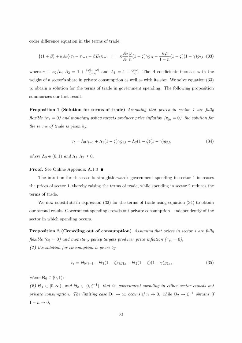
order difference equation in the terms of trade:

{(1 + β) + κA2} τt − τt−1 − βEtτt+1 = κA2

A1

ϕ

n(1− ζ)γg1t −

κϕ

1− n(1− ζ)(1− γ)g2,t, (33)

where κ ≡ κ2/n, A2 = 1 + ζϕ(1−ω)1−n and A1 = 1 + ζϕω

n . The A coefficients increase with the

weight of a sector’s share in private consumption as well as with its size. We solve equation (33)

to obtain a solution for the terms of trade in government spending. The following proposition

summarizes our first result.

Proposition 1 (Solution for terms of trade) Assuming that prices in sector 1 are fully

flexible (α1 = 0) and monetary policy targets producer price inflation (πyt = 0), the solution for

the terms of trade is given by:

τt = Λ0τt−1 + Λ1(1− ζ)γg1,t − Λ2(1− ζ)(1− γ)g2,t, (34)

where Λ0 ∈ (0, 1) and Λ1,Λ2 ≥ 0.

Proof. See Online Appendix A.1.3

The intuition for this case is straightforward: government spending in sector 1 increases

the prices of sector 1, thereby raising the terms of trade, while spending in sector 2 reduces the

terms of trade.

We now substitute in expression (32) for the terms of trade using equation (34) to obtain

our second result. Government spending crowds out private consumption—independently of the

sector in which spending occurs.

Proposition 2 (Crowding out of consumption) Assuming that prices in sector 1 are fully

flexible (α1 = 0) and monetary policy targets producer price inflation (πyt = 0),

(1) the solution for consumption is given by

ct = Θ0τt−1 −Θ1(1− ζ)γg1,t −Θ2(1− ζ)(1− γ)g2,t, (35)

where Θ0 ∈ (0, 1);

(2) Θ1 ∈ [0,∞), and Θ2 ∈ [0, ζ−1), that is, government spending in either sector crowds out

private consumption. The limiting case Θ1 → ∞ occurs if n → 0, while Θ2 → ζ−1 obtains if

1− n→ 0;

31

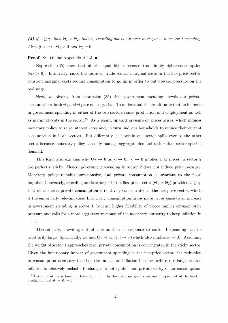
(3) if ω ≥ γ, then Θ1 > Θ2, that is, crowding out is stronger in response to sector 1 spending.

Also, if κ→ 0, Θ1 > 0 and Θ2 = 0.

Proof. See Online Appendix A.1.3

Expression (35) shows that, all else equal, higher terms of trade imply higher consumption

(Θ0 > 0). Intuitively, since the terms of trade reduce marginal costs in the flex-price sector,

constant marginal costs require consumption to go up in order to put upward pressure on the

real wage.

Next, we observe from expression (35) that government spending crowds out private

consumption: both Θ1 and Θ2 are non-negative. To understand this result, note that an increase

in government spending in either of the two sectors raises production and employment as well

as marginal costs in the sector.22 As a result, upward pressure on prices arises, which induces

monetary policy to raise interest rates and, in turn, induces households to reduce their current

consumption in both sectors. Put differently, a shock in one sector spills over to the other

sector because monetary policy can only manage aggregate demand rather than sector-specific

demand.

This logic also explains why Θ2 → 0 as κ → 0. κ → 0 implies that prices in sector 2

are perfectly sticky. Hence, government spending in sector 2 does not induce price pressure.

Monetary policy remains unresponsive, and private consumption is invariant to the fiscal

impulse. Conversely, crowding out is stronger in the flex-price sector (Θ1 > Θ2) provided ω ≥ γ,

that is, whenever private consumption is relatively concentrated in the flex-price sector, which

is the empirically relevant case. Intuitively, consumption drops more in response to an increase

in government spending in sector 1, because higher flexibility of prices implies stronger price

pressure and calls for a more aggressive response of the monetary authority to keep inflation in

check.

Theoretically, crowding out of consumption in response to sector 1 spending can be

arbitrarily large. Specifically, we find Θ1 →∞ if n→ 0 (which also implies ω → 0). Assuming

the weight of sector 1 approaches zero, private consumption is concentrated in the sticky sector.

Given the inflationary impact of government spending in the flex-price sector, the reduction

in consumption necessary to offset the impact on inflation becomes arbitrarily large because

inflation is relatively inelastic to changes in both public and private sticky-sector consumption.

22Except if utility is linear in labor (ϕ = 0). In this case, marginal costs are independent of the level ofproduction and Θ1 = Θ2 = 0.

32

Instead, when 1−n→ 0, crowding out of consumption in response to sector 2 spending, captured

by Θ2, does not exceed ζ−1. At this point, the drop in consumption matches the increase in

government spending in absolute value such that marginal costs, and hence inflation, remain

constant. This happens for a relatively modest reduction in consumption because inflation is

very elastic to changes in both public and private spending in the flexible sector.

Finally, we establish the effect of government spending on output.

Proposition 3 (Output multipliers) Assuming that prices in sector 1 are fully flexible (α1 =

0) and monetary policy targets producer price inflation (πyt = 0), the solution for output is given

by

yt = Γ0τt−1 + Γ1(1− ζ)γg1,t + Γ2(1− ζ)(1− γ)g2,t (36)

where Γ0 ∈ (0, 1), and

Γ1 = 1− ζΘ1 and Γ2 = 1− ζΘ2. (37)

Moreover, we find that Γ0 ∈ (0, 1), Γ1 has full support in (−∞, 1], and Γ2 has full support in

(0, 1].

In expression (36), the effect of the lagged terms of trade on output is positive (Γ0 > 0)

because, as discussed above, their effect on consumption is also positive (see Proposition 2). The

coefficients Γ1 and Γ2 directly capture the impact multiplier of government spending on output,

that is, the change in output divided by the change in government spending.23 Also, equation

(37) shows that the sum of the direct effect of higher spending on output and the indirect effect

on private consumption, which is negative, determine the overall multiplier.

Given our results regarding Θ1 and Θ2 in Proposition 2, it follows immediately that Γ1

may actually be negative: that is government spending may actually lower output—the fiscal

multiplier can be negative.24 On the other hand, Γ2 is bounded from below by zero, just as in

the one sector New Keynesian model. Moreover, we also stress the multiplier may not exceed

unity, again, just as in the one sector model unless the zero lower bound on interest rates binds

(Woodford, 2011).

23While gk,t measures the percentage deviation of government spending from its steady-state level, multiplyingwith (1 − ζ)γ and (1 − ζ)(1 − γ) transforms the expression into units of steady-state output.

24Baxter and King (1993) also obtain a negative multiplier in case taxes are distortionary. Instead, we assumethroughout that taxes are lump sum.

33

4.4 Model Simulations

We simulate the model in order to illustrate the quantitative relevance of our theoretical results

and to highlight the relevance of the five facts we establish. We start from a symmetric baseline

case for which we assume parameter values in line with the earlier literature as benchmark which

we summarize in the top panel of Table 4. We calibrate the model at the monthly frequency and

set β = 0.997, implying an annual interest rate in steady state of 3.6 percent. The inverse of the

Frisch elasticity is ϕ = 4 (see, e.g., Chetty et al., 2011). For the baseline model we assume both

sectors are perfectly homogeneous and of equal size: n = γ = 0.5. We set ρ1 = ρ2 = 0.85, in line

with estimates reported by Galı et al. (2007). We assume government spending accounts for 20

percent of output.25 Lastly, regarding the pricing friction we set α1 = α2 = 0.89, which implies

an average duration of price spells of 9 months. This degree of price stickiness corresponds to

the values in the most sticky sectors (see Section 3.5), a conservative choice as will become clear

below. Under these assumptions the model is perfectly symmetric and behaves like the standard

one-sector model.

We contrast the results of the symmetric baseline model with those of a model version which

captures—in a stylized way—the five facts. Table 4 summarizes the facts and how we consider

them in the model. Throughout, we calibrate sector 2 to capture key aspects regarding the top-3

most important supplying sectors to the federal government (two digit NAICS classification).

In line with fact 1, we set 1 − γ = 0.7 because these sectors jointly make up 70 percent of

government spending. Next, we set 1 − n = 0.18 because these sectors account for 18 percent

of GDP, implying ω = 0.95 and hence a large sectoral bias, consistent with fact 2: private

expenditure is biased towards sector 1, government spending is biased towards sector 2. To

account for fact 3, we set ρ1 = 0.37 and ρ2 = 0.45 such that government spending exhibits

less persistence than what is commonly assumed in the literature and differs slightly across

sectors.26 We consider fact 4 as we model distinct shocks, originating either in sector 1 or

in sector 2. Finally, we set the Calvo parameters in accordance with fact 5: α1 = 0.78 and

α2 = 0.89, implying an average duration of price spells of 4 months in sector 1 and 8.6 months

in sector 2.

Figure 7 shows the impulse responses for the baseline version of the model (solid blue line)

and contrasts them to those for the five-facts model (red line with circles). Panel A. shows the

25While our contract data cover only 16 percent of general government spending, the evidence above suggeststhat they are representative of government spending more generally, including the state and local level.

26We show extensive robustness results below.

34

Table 4: Model Parameters and the Five Facts

Baseline: symmetric modelβ 0.997 Monthly discount factorϕ 4 Inverse of Frisch elasticityn 0.5 Equally sized sectorsγ 0.5 Government consumption spread equally across sectorsρg1 0.85 Persistence parameter shock process: sector 1ρg2 0.85 Persistence parameter shock process: sector 2gy 0.2 Share of government spending in outputα1 0.89 Freq. of price changes: 11%α2 0.89 Freq. of price changes: 11%

Fact 1: Government spending is granular1− γ 0.7 Sector 2 represents top-3 two-digit NAICS sectors

Fact 2: Government spending is sectorally biased1− n 0.18 Top-3 two-digit NAICS sectors account for 18 percent of GDP

Fact 3: Government spending is characterized by short contract durationsρ1 0.37 Average persistence excl. top-3 two-digit NAICS sectorsρ2 0.45 Average persistence in top-3 two-digit NAICS sectors

Fact 4: Idiosyncratic shocks drive aggregate variation over timeε1 1pp Sector-1 shock: one percent of GDPε2 1pp Sector-2 shock: one percent of GDP

Fact 5: Government spending is concentrated in sticky sectorsα1 0.78 Freq. of price changes excl. top-3 two-digit NAICS sectors: 22%α2 0.89 Freq. of price changes in top-3 two-digit NAICS sectors: 11%

response to a shock originating in sector 1 and Panel B. shows the response to a shock originating

in sector 2. Here and in what follows we normalize the size of the shock to one percent of steady-

state output. Horizontal axes measure time in months, vertical axes measure deviations from

steady state in percent. In the baseline model, the response of aggregate output is independent

of where the shock originates because sectors are homogeneous. Moreover, because monetary

policy pursues a strict inflation target, the output effects of a shock to government spending are

rather moderate: the impact multiplier is slightly above 0.2.

A different picture emerges for the five-facts model. The impact multiplier of a sector-1

shock is slightly reduced relative to the baseline, but amounts to almost 0.8 for a sector-2 shock.

To understand the changes in the transmission mechanism, we consider the facts in isolation:

starting from the baseline, we progressively account for one additional fact at a time. Since

35

Figure 7: Effects of Government Spending Shocks on Aggregate Output

A. Sector-1 shock B. Sector-2 shock

Notes: Shock equals one percent of steady-state output in each scenario; horizontal axis: time in months, vertical

axis: deviation from steady state. Blue solid line correspond to symmetric baseline model. Black dashed

line: symmetric model except for heterogeneous pricing friction; green dotted line: symmetric model except

for heterogeneous pricing friction and γ = n = 0.3, magenta dashed-dotted line: as before but with n = 0.82; red

line with circles: five facts model.

the facts interact, the ordering in which they are introduced is important. In fact, unless price

stickiness differs across sectors, sectoral heterogeneity has a moderate impact on the transmission

mechanism. We therefore account for heterogeneous pricing frictions first. Black dashed lines

show the results: output drops in response to a sector-1 shock—a negative multiplier—and

increases much more strongly in response to a sector-2 shock. We established in Proposition 3

the possibility of an output decline in response to a sector-1 shock. We now see that it occurs

even though the degree of price stickiness in sector-1 is not particularly low (α1 = 0.78), but

lower than in sector 2 (α2 = 0.89).

We investigate how the degree of price stickiness shapes aggregate dynamics more

systematically in Panel A. of Figure 8. Here we display the impact response of output for

alternative values of α1, measured along the horizontal axis. Moving to the right means that

price stickiness in sector 1 increases, while we keep constant the pricing friction in sector 2 at

α2 = 0.89. For a wide range of parameter values of α1 the output effect of a sector-1 shock

given by the solid blue line is negative, reflecting strong crowding out of private consumption.

Raising the pricing friction in sector 1 mitigates this effect, but only moderately so unless α1

assumes large values. At the same time, raising α1 lowers the output response to a sector-2

shock, shown by the dashed red line, consistent with the analytical results in Section 4.3: as

36

Figure 8: Impact Multipliers for Alternative Parameter Values

A. Pricing friction Sector 1 B. Granularity

Notes: Impact response of output (measured along vertical axis in percent deviations from steady state output)

to government spending shock originating in sector 1 (solid line) vs sector 2 (dashed line). Shocks are normalized

to be equal to one percent of steady state output. Panel A. shows impact multipliers for alternative values of α1,

measured along the horizontal axis. α = 0.89 and other parameter values as in the symmetric baseline model.

Panel B. shows impact multipliers for various degrees of granularity. In this case we set α1 = 0.78 and α2 = 0.89.

sector 1 becomes more sticky, monetary policy has to compress consumption more in order to

stabilize inflation in response to a sector-2 shock. Hence, the multiplier decreases in the overall

degree of price stickiness in the economy, and increases in the relative stickiness of the sector in

which government spending rises.

Granularity is another key determinant for (the sign of) the output response to a sector-1

shock. If spending, both private and public, is concentrated in sector 2, a scenario represented

by the green dotted line in Figure 7, then output drops even more strongly in response to a

sector-1 shock. Panel B. of Figure 8 illustrates systematically how varying the weight of sector 1

in the economy, n (through a simultaneous adjustment of ω and γ), from zero to one alters the

impact effect of fiscal shocks on output. The blue solid line represents the effect of a sector-1

shock and the red dashed line the effect of a sector-2 shock. We observe that the smaller sector

1, the smaller the effect of both shocks, because more spending is concentrated in the relatively

sticky sector 2 and monetary policy has to engineer a larger contraction to stabilize inflation.

The magenta dash-dotted line in Figure 7 shows the output response in case we consider

sectoral bias in addition to the other facts. Relative to the scenario captured by the green dotted

lines, private spending is now concentrated in sector 1 where prices are much more flexible. As

a result, a spending increase in sector 1 is now expansionary, since a smaller decline of private

37

Figure 9: Response to Sector-2 Shock

A. Interest rate B. Markups

Notes: Impulse responses to Sector-2 shock. Shock is equal to one percent of steady-state output. Horizonal axis

measures time in quarters. Vertical axis measures deviation from pre-shock level in percentage points (interest

rate) and percent (markup).

consumption is sufficient to stabilize inflation. The difference for the effect of a sector-2 shock

is moderate. Lastly, once we change the persistence of the shock process we obtain much more

short-lived and relatively front-loaded effects of both shocks.

The predictions of the five-facts model differ from those of the symmetric baseline not only

in terms of output, but also along other dimensions. To illustrate these differences, we show in

Figure 9 the impulse response of the interest rate (Panel A.) and the markup in sector 1 (Panel

B.) to a government spending shock in sector 2. Here, we focus on a sector 2 shock because

sector 2 is the sector in which government spending is concentrated. The response of the interest

rate is muted in the five-facts model (red line with circles) compared to the symmetric baseline

(blue solid line), even though the shock is less persistent. For the sake of comparison, we also

plot the symmetric baseline model but assume that the persistence of the shock is the same as

in the five-facts model (ρ2 = 0.45). Compared to this benchmark, the response of the interest

rate in the five facts model is only one fifth. Intuitively, when government spending is biased

towards the sector with stickier prices, less crowding out of private consumption is necessary to

keep inflation stable. And indeed, several time-series studies find the responses of inflation and

interest rates to government spending shocks are moderate, or even negative (Mountford and

Uhlig, 2009; Corsetti et al., 2012; Ramey, 2016). As our model simulations show, accounting for

the heterogeneity in government spending goes some way towards accounting for these findings.

38

The markup response is another dimension along which our two-sector New-Keynesian

model shows an improved performance relative to the one-sector model. The basic one-sector

model predicts a markup decline in response to government spending shocks—a prediction at

odds with evidence (Nekarda and Ramey, 2011, 2013, 2020). In the two-sector model, we obtain

a more nuanced picture. If the shock originates in sector 2, markups in sector 2 decline, but

they increase in sector 1, which we show Panel B. of Figure 9. Intuitively, higher government

spending in sector 2 pushes up marginal costs in sector 2, which induces a decline of the markup

because prices adjust only sluggishly. But since the marginal utility of wealth declines, labor

supply increases in both sectors, causing a drop in marginal costs in sector 1 and an increase

of the markup. This effect is symmetric in the baseline model. In the five-facts model, the

drop in sector-2 markups is larger than the increase of sector-1 markups because of differential

price stickiness. Depending on where shocks originate, markups can be either pro-cyclical or

counter-cyclical at the aggregate level depending on how sectors are aggregated. It is crucial

to deviate from a one-sector model to arrive at these insights which help explain the empirical

difficulties in identifying a clear sign in the measured markup responses (e.g., Born and Pfeifer,

2021).

4.5 Alternative Model Specifications

We now show our main results are robust across a number of alternative model specifications.

In each instance, we show the response of output in Figure 10. As before, Panel A. displays

the response to a shock originating in sector 1, whereas Panel B. displays those to a shock

in sector 2. First, we consider an alternative specification for monetary policy. So far, we

assumed monetary policy follows a strict inflation target. Because monetary policy is key for

the fiscal transmission mechanism, we verify our main results also holds once we assume simple

interest-rate feedback rules for monetary policy. Specifically, we assume that the policy rate

adjusts to inflation with a response coefficient of 1.5. Relative to strict inflation targeting,

this rule implies a somewhat more accommodative monetary stance in the face of government

spending shocks, which results in a larger output response relative to the baseline five-facts

model (compare blue solid and red-circle lines in Panel A of Figure 10). The difference in the

responses across shocks originating in differnet sectors is now less pronounced, but still sizable

(compare blue solid line across panels).

Because of the importance of monetary policy and the interaction with price stickiness for

39

Figure 10: Effects of Government Spending Shocks on Aggregate Output

A. Sector-1 shock B. Sector-2 shock

Notes: Shock equals one percent of steady-state output in each scenario; horizontal axis: time in months, vertical

axis: deviation from steady state. Red lines with circles represent five-facts model as introduced in Figure 7, blue

solid line represents Taylor rule scenario, dashed line in magenta correspond to ELB scenario, black dashed line

to higher persistence of shock process, green dotted line DoD calibration.

the fiscal transmission mechanism, we also consider the case when the effective lower bound

(ELB) on interest rates binds. In this case, higher government spending does not trigger an

increase in interest rates: private consumption is crowded in and the fiscal multiplier is larger

than in normal times—a result well known from one-sector models (Eggertsson, 2011; Christiano

et al., 2011). We revisit this case in our two-sector model. Specifically, a shock to the time-

discount factor increases households’ desire to save such that the economy is pushed to the ELB

for three months.27 The dashed lines in magenta in Figure 10 show the impact of fiscal shocks,

assuming a Taylor rule (and an ELB at zero). Because the Taylor rule would call for lower rates

in response to the discount factor shock, interest rates do not increase (as in normal times) in

response to the fiscal shocks.28 As a result, private consumption is now increasing on impact in

response to the shocks and the multiplier exceeds unity just as in the one-sector model.

The new aspect of our analysis is that the ELB impacts the economy differently depending

on where the fiscal shock originates. Relative to our baseline without binding ELB, a sector-1

shock results in a larger output response than a shock in sector 2 because higher government

27We solve the model while allowing for an occasionally binding ELB constraint using the OccBin toolkit ofGuerrieri and Iacoviello (2015).

28The fiscal impulse is small enough and does not change the duration for which the ELB binds even though,in principle, the exit from the ELB is endogenous and may be quicker if the fiscal stimulus is large (Erceg andLinde, 2014).

40

spending in sector 1 has a stronger inflationary impact. In normal times, the inflationary

pressure would trigger a stronger monetary contraction, which does not take place at the ELB.

The stronger inflationary impulse therefore translates into a stronger drop in the real interest rate

and, eventually, a stronger crowding in of private consumption. Conversely, the ELB provides

little amplification in the case of the sector-2 shock because prices are more sticky in sector

2. Since government spending is concentrated in sector 2, our results are in line with recent

evidence which suggests that fiscal shocks are not substantially amplified at the ELB (Ramey

and Zubairy, 2018).

In theory, the persistence of fiscal shocks is an important parameter for the fiscal

transmission mechanism because of the implied wealth effect (Baxter and King, 1993). For this

reason, we also run the five-facts model assuming higher persistence parameters. Specifically,

we set ρg1 = 0.97 and ρg2 = 0.96. These values correspond to the average estimates in the top 3

two-digit NAICS sectors and the remaining sectors, respectively, once we employ an X13 filter

to remove the seasonality in the time series of the contract data (see our discussion of fact 3).

The black dashed lines in Figure 10 show the results. The impact responses are unchanged for

output and consumption relative to the baseline (shown by the red line with circles), but the

adjustment is much more persistent.29

In a last experiment, we assess whether calibrating the government sector to DOD-contract

data makes a difference (relative to the baseline which uses all contract data). Specifically, in

this case, we set γ = 0.27 and n = 0.77, α1 = 0.72, and α2 = 0.84. These values differ because

the top three 2-digit NAICS sectors differ from our baseline setup (see fact 2). We find the

adjustment to fiscal shocks for this calibration, shown by the green dotted line in Figure 10, is

very similar to the responses for the basic five-facts model.

5 Conclusion

In this paper, we provide an anatomy of Big G. A systematic analysis of the universe of

procurement contracts of the U.S. federal government, complemented by analyses of state and

local spending based on BEA input-output tables, allows us to establish five facts about the

nature of government spending. Accounting for these facts helps improve our understanding of

29We note, however, that our model does not feature capital in production. In Baxter and King (1993), thewealth effect alters labor supply and hence capital accumulation through which the shock persistence has a first-order effect on the fiscal transmission mechanism. In a more recent analysis, Boehm (2020) finds that short-livedgovernment investment shocks generate a smaller fiscal multiplier than government consumption shocks.

41

how fiscal policy works. As a first step in this direction, we calibrate a simple two-sector New

Keynesian model that captures the five facts in a stylized fashion.

The fiscal transmission mechanism in the micro-founded two-sector model differs consid-

erably from the one-sector model. While private expenditure is crowded out independently of

where the shock originates, crowding out can become arbitrarily large if the shock hits the sector

in which private expenditure is concentrated and prices are flexible—up to the point where the

fiscal multiplier turns negative. Crowding out, instead, is limited in the case in which the shock

hits the sticky sector. In this case, the output multiplier is also considerably larger, by a factor

of four. We leave a more systematic quantitative exploration for future work.

References

Acconcia, A., G. Corsetti, and S. Simonelli (2014, July). Mafia and public spending: Evidence onthe fiscal multiplier from a quasi-experiment. American Economic Review 104 (7), 2185–2209.

Acemoglu, D., V. M. Carvalho, A. Ozdaglar, and A. Tahbaz-Salehi (2012). The network originsof aggregate fluctuations. Econometrica 80 (5), 1977–2016.

Auclert, A., M. Rognlie, and L. Straub (2018, September). The intertemporal Keynesian cross.Working Paper 25020, National Bureau of Economic Research.

Auerbach, A. J., Y. Gorodnichenko, and D. Murphy (2020). Local fiscal multipliers and fiscalspillovers in the usa. IMF Economic Review 68, 195–229.

Baqaee, D. R. and E. Farhi (2020, February). Productivity and misallocation in generalequilibrium. The Quarterly Journal of Economics 135 (1), 105–163.

Barsky, R., C. L. House, C. Boehm, and M. S. Kimball (2016). Monetary policy and durablegoods. Working Paper 2016-18, Federal Reserve Bank of Chicago.

Barsky, R. B., C. L. House, and M. S. Kimball (2007, June). Sticky-price models and durablegoods. American Economic Review 97 (3), 984–998.

Baxter, M. and R. G. King (1993, June). Fiscal Policy in General Equilibrium. AmericanEconomic Review 83 (3), 315–334.

Bigio, S. and J. La’o (2020). Distortions in production networks. QJE 135 (4), 2187–2253.

Blanchard, O., C. J. Erceg, and J. Linde (2017). Jump-Starting the Euro-Area Recovery: Woulda Rise in Core Fiscal Spending Help the Periphery? NBER Macroeconomics Annual 31 (1),103–182.

Boehm, C. E. (2020). Government consumption and investment: Does the composition ofpurchases affect the multiplier? Journal of Monetary Economics 115, 80 – 93.

Born, B. and J. Pfeifer (2021). Uncertainty-driven business cycles: assessing the markup channel.Quantitative Economics 81 (2), 587–623.

Bouakez, H., O. Rachedi, and S. Emiliano (2020, December). The sectoral origins of the spendingmultiplier. Working paper.

Carvalho, C., J. W. Lee, and W. Y. Park (2021, January). Sectoral price facts in a sticky-pricemodel. American Economic Journal: Macroeconomics 13 (1), 216–56.

Chetty, R., A. Guren, D. Manoli, and A. Weber (2011). Are micro and macro labor supplyelasticities consistent? American Economic Review 101 (3), 471–475.

42

Chodorow-Reich, G. (2019, May). Geographic cross-sectional fiscal spending multipliers: Whathave we learned? American Economic Journal: Economic Policy 11 (2), 1–34.

Christiano, L. J., M. Eichenbaum, and S. Rebelo (2011). When is the government spendingmultiplier large? Journal of Political Economy 119 (1), 78–121.

Cohen, L., J. Coval, and C. Malloy (2011, December). Do powerful politicians cause corporatedownsizing? Journal of Political Economy 119 (6), 1015–1060.

Corsetti, G., A. Meier, and G. J. Muller (2012, November). Fiscal stimulus with spendingreversals. The Review of Economics and Statistics 94 (4), 878–895.

Decarolis, F., L. M. Giuffrida, E. Iossa, V. Mollisi, and G. Spagnolo (2020, 05). BureaucraticCompetence and Procurement Outcomes. The Journal of Law, Economics, and Organization.

Demyanyk, Y., E. Loutskina, and D. Murphy (2019). Fiscal stimulus and consumer debt. TheReview of Economics and Statistics 101 (4), 728–741.

Dupor, B. and R. Guerrero (2017). Local and aggregate fiscal policy multipliers. Journal ofMonetary Economics 92, 16 – 30.

Eggertsson, G. B. (2011, January). What fiscal policy is effective at zero interest rates? InNBER Macroeconomics Annual 2010, Volume 25, pp. 59–112.

Erceg, C. and J. Linde (2014). Is there a fiscal free lunch in a liquidity trap? Journal of theEuropean Economic Association 12 (1), 73–107.

Erceg, C. J. and J. Linde (2012, May). Fiscal Consolidation in an Open Economy. AmericanEconomic Review 102 (3), 186–191.

Farhi, E. and I. Werning (2016). Fiscal multipliers. In J. B. Taylor and H. Uhlig (Eds.), Handbookof Macroeconomics, Volume 2, Chapter 31, pp. 2417–2492. Elsevier.

Fisher, J. D. and R. Peters (2010). Using stock returns to identify government spending shocks*.The Economic Journal 120 (544), 414–436.

Foerster, A. T., P.-D. G. Sarte, and M. W. Watson (2011). Sectoral vs aggregate shocks: Astructural factor analysis. Journal of Political Economy 119 (1), 1–38.

Gabaix, X. (2011). The granular origins of aggregate fluctuations. Econometrica 79 (3), 733–772.

Galı, J. (2015, March). Monetary Policy, Inflation, and the Business Cycle: An Introduction tothe New Keynesian Framework and Its Applications. Princeton University Press.

Galı, J., J. D. Lopez-Salido, and J. Valles (2007, March). Understanding the effects ofgovernment spending on consumption. JEEA 5 (1), 227–270.

Galı, J. and T. Monacelli (2008, September). Optimal monetary and fiscal policy in a currencyunion. Journal of International Economics 76 (1), 116–132.

Gilchrist, S., R. Schoenle, J. Sim, and E. Zakrajsek (2017, March). Inflation dynamics duringthe financial crisis. American Economic Review 107 (3), 785–823.

Guerrieri, L. and M. Iacoviello (2015). OccBin: A toolkit for solving dynamic models withoccasionally binding constraints easily. Journal of Monetary Economics 70, 22–38.

Hagedorn, M., I. Manovskii, and K. Mitman (2019, February). The fiscal multiplier. WorkingPaper 25571, National Bureau of Economic Research.

Hebous, S. and T. Zimmermann (2021). Can government demand stimulate private investment?evidence from u.s. federal procurement. Journal of Monetary Economics 118, 178–194.

Hettig, T. and G. J. Muller (2018). Fiscal policy coordination in currency unions at the effectivelower bound. Journal of International Economics 115 (C), 80–98.

Kaplan, G., B. Moll, and G. L. Violante (2018, March). Monetary policy according to HANK.American Economic Review 108 (3), 697–743.

43

La’O, J. and A. Tahbaz-Salehi (2020). Optimal monetary policy in production networks.Technical report, National Bureau of Economic Research.

Leeper, E. M., T. B. Walker, and S.-C. S. Yang (2013). Fiscal foresight and information flows.Econometrica 81 (3), 1115–1145.

McKay, A., E. Nakamura, and J. Steinsson (2016, October). The power of forward guidancerevisited. American Economic Review 106 (10), 3133–3158.

McKay, A. and R. Reis (2016). The role of automatic stabilizers in the U.S. business cycle.Econometrica 84 (1), 141–194.

Mountford, A. and H. Uhlig (2009, September). What are the effects of fiscal policy shocks?Journal of Applied Econometrics 24 (6), 960–992.

Nakamura, E. and J. Steinsson (2014, March). Fiscal stimulus in a monetary union: Evidencefrom US regions. American Economic Review 104 (3), 753–792.

Nekarda, C. J. and V. A. Ramey (2011, January). Industry evidence on the effects of governmentspending. American Economic Journal: Macroeconomics 3 (1), 36–59.

Nekarda, C. J. and V. A. Ramey (2013, June). The cyclical behavior of the price-cost markup.Working Paper 19099, National Bureau of Economic Research.

Nekarda, C. J. and V. A. Ramey (2020). The cyclical behavior of the price-cost markup. Journalof Money, Credit, and Banking, forthcoming.

Ozdagli, A. and M. Weber (2017, May). Monetary policy through production networks: Evidencefrom the stock market. Working Paper 23424, National Bureau of Economic Research.

Pasten, E., R. Schoenle, and M. Weber (2019a). Price rigidities and the origins of aggregatefluctuations. Unpublished manuscript, University of Chicago.

Pasten, E., R. Schoenle, and M. Weber (2019b, October). Production networks and thepropagation of monetary policy shocks. Journal of Monetary Economics. in press.

Ramey, V. A. (2011, September). Can government purchases stimulate the economy? Journalof Economic Literature 49 (3), 673–685.

Ramey, V. A. (2016, February). Macroeconomic shocks and their propagation. Working Paper21978, National Bureau of Economic Research.

Ramey, V. A. (2019). Ten years after the financial crisis: What have we learned from therenaissance in fiscal research? Journal of Economic Perspectives 33 (2), 89–114.

Ramey, V. A. and M. D. Shapiro (1998, June). Costly capital reallocation and the effects ofgovernment spending. Carnegie-Rochester Conference Series on Public Policy 48, 145–194.

Ramey, V. A. and S. Zubairy (2018, April). Government spending multipliers in good times andin bad: evidence from US historical data. Journal of Political Economy 126 (2), 850–901.

Rubbo, E. (2020). Networks, phillips curves, and monetary policy. Manuscript .

Svensson, L. E. O. (2003, June). What is wrong with Taylor rules? Using judgment in monetarypolicy through targeting rules. Journal of Economic Literature 41 (2), 426–477.

Woodford, M. (2003). Interest and Prices. Princeton University Press.

Woodford, M. (2011). Simple analytics of the government expenditure multiplier. AmericanEconomic Journal: Macroeconomics 3 (1), 1–35.

Woodford, M. (2020). Effective demand failures and the limits of monetary stabilization policy.Discussion Paper 15211, CEPR.

44

Online Appendix:

Big G

Lydia Cox, Gernot J. Muller, Ernesto Pasten, Raphael Schoenle, and Michael Weber

Not for Publication

A.1.1 Steady State

We consider a symmetric steady state where relative prices are unity and inflation is zero.

However, note that the size of sectors will generally differ in the steady state. We show below

conditions for the existence of a symmetric steady state across firms in which the following holds:

Wk = W, Pjk = P for all j, k

Symmetry in prices across all firms implies

P = P k

such that from eqs. (2) and (4) we have

C1 = ωC,C2 = (1− ω)C,

nYj1 = Y1, (1− n)Yj2 = Y2.

Note that while sectors differ in size, the level of steady-state production is the same across

firms. For sectoral output we have

Y1 = C1 +G1, Y2 = C2 +G2 (A.1)

Adding these gives

Y1 + Y2 = ωC + (1− ω)C +G1 +G2 = C +G1 +G2 = Y (A.2)

where the last equation follows from the definition of real GDP. In the symmetric steady state

we have

G = G1 +G2

1

such that we can define the sectoral shares of public spending as follows

γ ≡ G1

Gand 1− γ =

G2

G.

Regarding the size of the sectors note that n = Y1/Y and 1− n = Y2/Y . This implies for labor

L1 = nL and L2 = (1 − n)L. Last define the share of private and public consumption in GDP

as follows

ζ =C

Yand 1− ζ =

G

Y

We thus write the following restriction

n =Y1

Y=ωC + γG

Y= ωζ + γ(1− ζ)

1− n =Y2

Y=

(1− ω)C + (1− γ)G

Y= (1− ω)ζ + (1− γ)(1− ζ)

The steady-state labor supply from equation (6) is

Wk

P= ξ1(nL)ϕC = ξ2((1− n)L)ϕC

For the symmetric steady state to exist it is sufficient that ξ1 = n−ϕ and ξ2 = (1− n)−ϕ. As a

result we have for labor supply in the steady state

W

P= LϕC. (A.3)

Households’ budget constraint, firms’ profits, production function, and optimal prices in

the steady state are, respectively,

CP + P1G1 + P2G2 = WL+ Π (A.4)

Π = P1Y1 + P2Y2 −WL = PY −WL (A.5)

Y = L (A.6)

P =θ

θ − 1W. (A.7)

2

From (A.7) we haveW

P=

(θ − 1

θ

)(A.8)

This in turn impliesΠ

P=

1

θY.

A.1.2 Note on Linearization of Phillips Curve

To derive the NKPC rewrite the first order condition of the firm (10) in the main text as follows

∞∑τ=0

Qt,t+τατk

P ∗ktYjkt+τPkt

=M∞∑τ=0

Qt,t+τατkYjkt+τ

Ψkt+τ

Pkt+τ

Pkt+τPkt

Note that here we divide both sides with the sectoral price level. Linearizing around the

symmetric steady state gives

∞∑τ=0

(βαk)τ [p∗kt − pkt + yjkt+τ ] =

∞∑τ=0

(βαk)τ [yjkt+τ + ψkt+τ + pkt+τ − pkt]

here ψkt+τ is the deviation of real marginal costs from the steady state (where marginal costs

are deflated with Pkt). Rewriting

1

1− αkβ[p∗kt − pkt] =

∞∑τ=0

(βαk)τ

[ψkt+τ +

τ−1∑l=0

πk,t+1+l

]

Using∑∞

τ=0(βαk)τ∑τ−1

l=0 πk,t+1+l = αkβ1−αkβ

∑∞τ=0(βαk)

τπkt+1+τ we can rewrite the previous

equation as follows

[p∗kt − pkt] = (1− αkβ)∞∑τ=0

(βαk)τψkt+τ + αkβ

∞∑τ=0

πkt+1+τ

Writing this in difference form

[p∗kt − pkt] = βαk[p∗kt+1 − pkt+1

]+ (1− βαk)ψkt + αkβπkt+1

From the definition of the price level in sector k we have: p∗kt − pkt = αk1−αkπkt Hence, we obtain

πkt = βEtπkt+1 +(1− αk)(1− βαk)

αkψkt

3

A.1.3 Proofs

A.1.3.1 Proposition 1

Proof of proposition 1. Substituting the solution (34) in (33) yields the conditions for the

unknown coefficients:

βΛ20 − {(1 + β) + κ [A2]}Λ0 + 1 = 0

{(1 + β) + κA2}Λ1 = βΛ0Λ1 + βΛ1ρ+ κA2

A1

ϕ

n

{(1 + β) + κA2}Λ2 = βΛ0Λ2 + βΛ2ρ+ κϕ

1− n

Let

f(x) = βx2 − {1 + β + κA2}x+ 1. (A.9)

This is a quadratic equation, with evaluation f(Λ0)→∞ if Λ0 →∞ or Λ0 → −∞. Plugging in

Λ0 = 0, we obtain that f(0) = 1. Plugging in Λ0 = 1, we obtain that

f(1) = β − [(1 + β) + κA2] + 1 = −κA2 < 0 (A.10)

Therefore the two roots of the quadratic equations lie within (0, 1) and (1,∞). The unique and

stable root is Λ0 ∈ (0, 1). Since we know that the root we seek is the smaller of the two, the

desired Λ0 is decreasing in κ(

1 + ζϕ(1−ω)1−n

).

Next we need to solve for Λ1 and Λ2. Then, we plug the results into the system and solve

directly:

Λ1 =κA2A1

ϕn

{(1 + β) + κA2} − β(Λ0 + ρ)≥ 0 (A.11)

The denominator of Λ1 is positive since β(Λ0 + ρ) < 2β < 1 + β.

Similarly

Λ2 =κ ϕ

1−n{(1 + β) + κA2} − β(Λ0 + ρ)

≥ 0 (A.12)

4

A.1.3.2 Proposition 2

Proof of (1), solution for consumption

Recall that ct can be written as

ct = (1− ω)τt −(

1 +ζϕω

n

)−1

(1− ζ)γϕ

ng1t (A.13)

Plugging in for τt as derived from Proposition 1

ct = (1−ω)Λ0τt−1 +(1−ω)(1−ζ)[Λ1γg1,t−Λ2(1−γ)g2,t]−(

1 +ζϕω

n

)−1

(1−ζ)γϕ

ng1t (A.14)

Combining (A.14) with the expression for b and c in (A.11) and (A.12) yields

ct = (1−ω)Λ0τt−1 +1− ζζ

[κ(1− ω)(A2

A1

ϕnγg1 − ϕ

1−n(1− γ)g2)

{(1 + β) + κA2} − β(Λ0 + ρ)−(

1 +ζϕω

n

)−1

γϕ

ng1

](A.15)

Let

ct = Θ0τt−1 −Θ1(1− ζ)γg1t −Θ2(1− ζ)(1− γ)g2t (A.16)

Thus, the lag coefficient on the previous period’s terms of trade τt−1 is

Θ0 = (1− ω)Λ1 (A.17)

where recall that Λ0 ∈ (0, 1) is the root of equation (A.9). Thus Θ0 ∈ (0, 1) as well.

The rest of (A.15) can be decomposed into the coefficient of consumption wrt government

spending in sector 1, Θ1:

Θ1 =ϕ

A1n− (1− ω)Λ1 =

ϕ

A1n− (1− ω)

κA2A1

ϕn

{(1 + β) + κA2} − β(Λ0 + ρ)(A.18)

Θ1 =ϕ

A1n

(1 + β) + ωκA2 − β(Λ0 + ρ)

{(1 + β) + κA2} − β(Λ0 + ρ)(A.19)

And the multiplier for consumption in sector 2, Θ2, is:

Θ2 = (1− ω)Λ2 =(1− ω)κ ϕ

1−n{(1 + β) + κA2} − β(Λ0 + ρ)

(A.20)

Proof of (2), the support of Θ1 and Θ2

5

From equations (A.19) and (A.20), it is immediate that both Θ1 and Θ2 are greater than

or equal to 0. The lower bound 0 can be attained by setting ϕ = 0.

Next we show that Θ1 is unbounded above. From (A.19), plugging in for A1 and A2,

Θ1 =ϕ(

1 + ζϕωn

)n

(1 + β) + ωκA2 − β(Λ0 + ρ)

{(1 + β) + κA2} − β(Λ0 + ρ)(A.21)

Consider an example where ζ, ϕ, κ 6= 0. As n → 0, it must be that ω → 0 as well. Then

ϕ/(n+ ζϕω)→∞, and Θ1 →∞ as well. Thus the support of Θ1 is between [0,∞).

Finally, we show that Θ2 is bounded above by ζ−1. From (A.20), plugging in for A2, and

multiplying by ζ on both sides,

ζΘ2 =ζ(1− ω)κ ϕ

1−n

(1 + β) + κ(

1 + ζϕ(1−ω)1−n

)− β(Λ0 + ρ)

(A.22)

As 1 + β + κ − β(Λ0 + ρ) > 0, the numerator of ζΘ2 is always less than the denominator.

Thus ζΘ2 ≤ 1. Next, when 1 − n → 0, ζΘ2 → 1. Therefore, the support of Θ2 is between

[0, ζ−1). It follows immediately that Θ2 → 0 for κ→ 0.

Proof of (3), Comparative statics between Θ1 and Θ2

The terms Θ1 and Θ2 are compared in equations (A.19) and (A.20).

Again, plugging in for A1 and A2, Θ1 > Θ2 if

[κ1− n+ ζϕ(1− ω)

1− nωϕ+A1(1 + (1− a− ρ)β)n](1− n) > κ

n+ ζϕω

n(1− ω)ϕn (A.23)

Since Λ0, ρ, β < 1, it’s clear that (1 + (1−Λ0− ρ)β) > 0, with emphasis on the strictness of the

inequality. Thus, inequality (A.23) holds if

[1− n+ ζϕ(1− ω)]ω ≥ [n+ ζϕω](1− ω) (A.24)

Simplifying further by dividing out (1 − w)w and canceling ζϕ, we obtain that a sufficient

condition such that Θ1 > Θ2 isω

n≥ 1− ω

1− n=⇒ ω > γ (A.25)

which implies that sector 1 is relatively more biased on the consumption side.

6

A.1.3.3 Proposition 3

Proof of Proposition 3. From the definition of output

yt = ny1,t + (1− n)y2,t

= ζct + (1− ζ)γg1,t + (1− ζ)(1− γ)g2,t

= ζ[Θ0τt−1 −Θ1(1− ζ)γg1,t −Θ2(1− ζ)(1− γ)g2,t] + (1− ζ)γg1,t + (1− ζ)(1− γ)g2,t

= ζΘ0τt−1 + (1− ζΘ1)(1− ζ)γg1t + (1− ζΘ2)(1− ζ)(1− γ)g2t.

Therefore, yt can be written as

yt = Γ0τt−1 − Γ1(1− ζ)γg1t − Γ2(1− ζ)(1− γ)g2t. (A.26)

As Γ0 = ζΘ0, and since ζ,Θ0 ∈ (0, 1), Γ0 ∈ (0, 1) as well.

We solve for the output multipliers Γ1 and Γ2 of sector 1 and sector 2 government spending,

respectively. Using equations (A.19) and (A.20) gives

Γ1 = 1− ζ · ϕ(1 + ζϕω

n

)n

(1 + β) + ωκA2 − β(Λ0 + ρ)

{(1 + β) + κA2} − β(Λ0 + ρ)︸ ︷︷ ︸Θ1

. (A.27)

To show that the support of Γ1 (−∞, 1], simply note that Θ1 has support between [0,∞), and

thus Γ1 = 1− ζΘ1 is unbounded on the left and upper bounded by 1.

Next, consider

Γ2 = 1− ζ(1− ω)κ ϕ

1−n

(1 + β) + κ(

1 + ζϕ(1−ω)1−n

)− β(Λ0 + ρ)︸ ︷︷ ︸

Θ2

(A.28)

Recall that Θ2 has support between [0, ζ−1), and thus Γ2 = 1− ζΘ2 has support (0, 1].

7

A.2 USASpending vs. Other Data in the Literature

While, to our knowledge, no one has employed the USASpending database in the way we do in

this paper, a number of papers make use of similar types of data on government spending. Most

recently, Auerbach et al. (2020) use part of the USASpending database in a more aggregated

fashion. Specifically, they use only contracts that originate at the US Department of Defense

(DOD). To extend their time series backward, they supplement the USASpending data on DOD

contracts with data that come directly from the Federal Procurement Data System (FPDS).

For their analysis, they aggregate the transaction-level data to create city-level measures of

federal defense spending. Nakamura and Steinsson (2014) also use data on defense procurement

contracts from an older database to compile data on total military procurement at the state

level from 1966 to 2006. The data that Nakamura and Steinsson (2014) employ are from the

DD Form 350, the procurement reporting form that preceded the FPDS forms that are in the

USASpending database and Auerbach et al. (2020) and so contain very comparable information

about the defense procurement contracts. The DOD transitioned from the DD Form 350 to

the FPDS in 2007. While Auerbach et al. (2020) aggregate to the city level, Nakamura and

Steinsson (2014) aggregate to the state level.1

Cohen et al. (2011) also look at a state-level measure of government spending, but these

authors use data on congressional earmarks—also known as “pork”—from Citizens Against

Government Waste (CAGW) to identify the impact of government spending on the private sector.

Instead of providing detailed information about the contract that the government enters into

with suppliers, as the USASpending data do, the earmark data show line items in appropriations

bills that are designated for specific purposes and are included in those bills in such a way that

circumvents the established budgetary procedure. Cohen et al. (2011) also use some data on

government procurement contracts from 1992-2008,2 aggregated at the state level.

1Since the inception of USASpending.gov, most other sources of federal government procurement data thatare published by government entities have now been transferred to the USASpending database, which links datafrom all around the federal government. Data are pulled directly from more than 100 federal agencies’ financialsystems, and pulled from other government systems like FPDS, the Federal Assistance Broker System (FABS),the FFATA Sub-award Reporting System (FSRS) and the System for Award Management (SAM).

2These data come from a private company called Eagle Eye.

8

A.3 Additional Results

This section reports additional results that we reference in the main body of the paper.

A.3.1 Largest Contracts in Top Sectors

To provide a bit more intuition as to what is “behind” the shocks that we estimate, we show the

five largest contracts awarded to the three largest sectors in terms of its share of government

contracts. These arrivals are behind the shock (though not the same, of course). Table A.1

shows the three largest transactions in NAICS 33 (manufacturing). Perhaps unsurprisingly,

since this is the manufacturing sector, the top contracts are all defense-related. Tables A.2 and

A.3 show the top contracts for NAICS 23 and NAICS 56, which are a bit broader in scope.

Table A.1: Ten Largest Transactions in NAICS33, Fiscal Year 2012

Action Date Recipient Amount Description

3/8/2012 The Boeing Company $3.37 B RSAF F-15 Fleet Modernization Program

6/6/2012 United Technologies Corporation $2.83 B Multi Service Contract for H60 Helicopters

1/31/2012 General Dynamics $2.71 B Construction of SSN 784

5/31/2012 Huntington Ingalls Industries, Inc. $2.16 B Award of LHA 7 Detail Design and Construction

6/22/2012 The Boeing Company $1.83 B F-15 S/SA Conversion & Provisioning

11/23/2011 Bell Boeing Joint Project Office $1.68 B Lot 16 MV Full Funding

9/21/2012 The Boeing Company $1.60 B Definitize P-8A LRIP III Aircraft

12/9/2011 Lockheed Martin Corporation $1.59 B Authorize efforts associated w/LRIP 5 Production

6/6/2012 The Boeing Company $1.24 B Definitization of India Aircraft

Table A.2: Five Largest Transactions in NAICS23, Fiscal Year 2012

Action Date Recipient Amount Description

9/28/2012 PCCP Constructors $625.9 M Permanent Canal Closures and Pumps

11/18/2011 Kiewit-Turner $580.2 M Price adj. for replacement med ctr (Aurora, CO).

9/24/2012 B.L. Harbert Holdings LLC $302.4 M New Embassy Compound, Jakarta, Indonesia

3/29/2012 Balfour Beatty/DPR/Big-D $221.0 M Utah Data Center (Camp Williams, UT).

1/13/2012 Hensel Phelps Constfuction CO $191.6 M Social Security Adinistration Nat’l Support Center

9

Table A.3: Five Largest Transactions in NAICS56, Fiscal Year 2012

Action Date Recipient Amount Description

7/31/2012 Lawrence Livermore Nat’l Security $7.86 B Mgmt/Oprtn, Lawrence Livermore Nat’l Lab

3/15/2012 S&K Aerospace LLC $1.24 B PROS IV (Tri-Service Technical Support)

6/18/2012 United Space Alliance, LLC $470.0 M Space Program Operations Contract

3/27/2012 Mission Essential Personnel, LLC $400.0 M Linguist Interpretation and Translation Services

9/30/2012 Hewlett-Packard Company $330.9 M Other ADP and Telecommunications Services

A.3.2 Granularity: Power Law Distribution

Government spending is granular in the sense that the distribution of government contracts is fat

tailed. In the main text we show that the full distribution is well approximated by a log-normal

distribution. Here, we show that a power law with shape parameter ζ < 2 also approximates

the distribution of government contracts well. The density of a simple power law is given by

f(x) = ζax−(ζ+1), so the log density is given by:

ln (f(x)) = −(ζ + 1) ln(x) + C

where C is a constant. Thus, when we plot the empirical log contract size against the log

frequency of that contract size, we should expect to see a straight line.

The left panel of Figure A.1 documents a linear relationship between the log size of firm

obligations and the log frequency when we use the top 20 percent of suppliers that supply

99 percent of government consumption. The right panel of the figure shows that the same

relationship also holds at the contract level (for the top 20 percent of contracts, which account

for 97 percent of government consumption).

Assuming the data do, indeed, follow a Pareto distribution, we can estimate the parameters

of the distribution via maximum likelihood. We estimate a shape parameter of ζ = 0.67, which

indicates fat tails. The estimated distribution provides a good fit to the data. Figure A.2 shows

the histogram of (the log of) contract obligations and the simulated probability density function

using the estimated parameters. When we compare the likelihood of the data under a Pareto

distribution and a log-normal distribution, the log-normal provides the better fit, which is why

we use it in the main text.

10

Figure A.1: Log Frequency vs. Log Contracts●

●

●

●

●

●

●

●

●

●

14 16 18 20 22 24

−8

−6

−4

−2

Log Firm Obligations

Log

Fra

ctio

n

(a) Top 20 Percent of Firms

●

●

●

●

●

●

●

●

●

●

●

●

12 14 16 18 20 22

−12

−10

−8

−6

−4

−2

Log Transaction Value

Log

Fra

ctio

n(b) Top 20 Percent of Transactions

Note. The left panel of this figure shows that there is a linear relationship between the log size of firm obligations and the

log frequency of that size. The right panel shows that the same is true for individual contract transactions. Showing that

there is a linear relationship between log-size and log-frequency is a simple way of showing that government contracts are

well-approximated by a power law.

Figure A.2: Histogram of Log Contracts and Simulated Probability Density Function

Log Obligations

Pro

babi

lity

0.0

0.1

0.2

0.3

0.4

0.5

11 12 13 14 15 16 17 18 19 20 21 22 23

Note. This figure shows a histogram of log contract transactions and the simulated density function of the associated

Pareto distribution with parameters estimated using MLE. We estimate a shape parameter of α = 0.67. Note that if

contracts are distributed Pareto(α, xm), the log contracts follow a two-parameter exponential distribution with

parameters (λ, θ), where λ = 1α

and θ = ln(xm).

11

A.3.3 Shock Structure of the Spending Process

Here, we examine the shock structure of the sectoral government spending process. Idiosyncratic

variation dominates this process, and these shocks are often strongly positively or negatively

correlated. To see this, we examine the shock structure of the following processes:

gs,t+1 = α0 + αs + αt + ρsgs,t + εs,t+1 (A.29)

where gs,t is the log of government consumption from two-digit sector s at time t. Variables αs

and αt take into account sectoral and aggregate time fixed effects. We calculate the residuals

εs,t and the variance-covariance matrix 1T ε′ε.

Our findings are twofold. First, we find that inclusion of time fixed effects in the specification

raises the R2 from 97.94 percent to only 98.34 percent. Hence, aggregate trends do not explain

much of sectoral variation over time; instead, idiosyncratic shocks are far more important,

accounting for almost four times as much of total variation. Second, we find that idiosyncratic

innovations can have large positive and negative correlations for many sector pairs. Figure A.3

shows the distribution of correlations across sector pairs. They are centered around 0, but can

be both large negative and positive. A lot of the correlation mass resides between -0.5 and 0.5.

Our previous cross-sectional variance decomposition (“Fact 1”) suggests that across-sector

variation is relatively unimportant. We note that our previous cross-sectional result is perfectly

consistent with the dynamic fact. When an innovation to sectoral spending occurs, it is often

strongly negatively or positively correlated with another sector’s spending level. The fat-tailed

distribution of individual contracts determines this finding.

12

Figure A.3: Density of Error Term Correlation Coefficients

−0.4 −0.2 0.0 0.2 0.4 0.6

0.0

0.5

1.0

1.5

2.0

2.5

Den

sity

Note. This figure shows the distribution of correlation across sector pairs that result from examining the

sectoral process: gs,t+1 = α0 + αs + αt + ρsgs,t + εs,t+1, where gs,t is the log of government consumption of

output from two-digit sector s in month t. The figure shows the distribution of the correlation coefficients of the

residuals for all sector pairs.

A.3.4 Decomposition of Government Spending Growth

Second, as in Foerster et al. (2011), we decompose changes in aggregate government spending

growth into components arising from aggregate and idiosyncratic (sector-specific) shocks.

Specially, we decompose aggregate government spending growth, Zt:

Zt =N∑i=1

ωi,tzi,t︸ ︷︷ ︸(1) Actual

=1

N

N∑i=1

zi,t︸ ︷︷ ︸(2) Equal Weights

+N∑i=1

(ωi −

1

N

)zi,t︸ ︷︷ ︸

(3) Granular Residual

+N∑i=1

(ωi,t − ωi)zi,t︸ ︷︷ ︸(4) Share Deviation

(A.30)

where i denotes two-digit NAICS sectors, ωi,t is sector i’s share of spending in year t, and ωi

is the average share of sector i in government spending for all years. The term (1/N)∑N

i=1 zit

weights each sector equally. If zit is uncorrelated, this component has a variance proportional

to N−1. The second term, the granular residual term,∑N

i=1 [ωit − (1/N)]it will be large if the

cross-sectional variance of sectoral shares is large at date t.

Figure A.7 plots the individual components of equation (A.30) over time. In Foerster et al.

(2011), the equally-weighted component tracks the series for aggregate industrial production

growth more closely than the granular residual term. In our case, both series exhibit fluctuations

13

of a magnitude similar to that of the aggregate growth rate, indicating that both idiosyncratic

shocks and covariance across sectors are important drivers of aggregate growth. We also find that

the granular residual is important in both defense and non-defense spending though it appears

to be larger and more volatile in defense spending (see Figure A.35 in the online appendix).

Furthermore, we show the importance of idiosyncratic innovations to the government

spending process by revisiting our sectoral AR(1) processes from the previous fact. As we show in

Online Appendix Section A.3.3, aggregate time fixed effects explain little of sectoral government

spending dynamics when included into the estimation. Instead, idiosyncratic innovations drive

changes in sectoral spending, which can have large positive and negative correlations across

sectors.

14

Figure A.4: Variance Decomposition: Within and Across Sectors0.

00.

20.

40.

60.

81.

0

Fiscal Year

Sha

re o

f Tot

al V

aria

nce

2001 2003 2005 2007 2009 2011 2013 2015 2017

WithinAcross

(a) Full Data Set

0.0

0.2

0.4

0.6

0.8

1.0

Fiscal YearS

hare

of T

otal

Var

ianc

e2001 2003 2005 2007 2009 2011 2013 2015 2017

WithinAcross

(b) Top 20 Percent

0.0

0.2

0.4

0.6

0.8

1.0

Fiscal Year

Sha

re o

f Tot

al V

aria

nce

2001 2003 2005 2007 2009 2011 2013 2015 2017

WithinAcross

(c) Bottom 80 Percent

Note. This figure shows a decomposition of the variance of government spending into “within-sector” and “across-sector”

variation. Specifically, total variation is given by:

∑s

∑f∈s

(gfs,t − gt)2 =∑s

∑f∈s

(gfs,t − gs,t)2︸ ︷︷ ︸Within Sector

+∑s

∑f∈s

(gs,t − gt)2

︸ ︷︷ ︸Across Sector

,

where f is a firm and s is a two-digit NAICS sector. We plot each of the two RHS components as a share of the LHS.

Panel (a) shows this decomposition for the full data set, panel (b) restricts the sample to the top 20 percent of firms, and

panel (c) shows only the bottom 80 percent of firms.

Figure A.5: Density of Variance Decomposition Components

−5 0 5 10 15 20 25

0.0

0.1

0.2

0.3

0.4

0.5

Den

sity Transactions

Avg.Sector ObligationsAvg. Annual Obligations

(a) Full Data Set

10 15 20 25

0.0

0.1

0.2

0.3

0.4

0.5

Den

sity Transactions

Avg.Sector ObligationsAvg. Annual Obligations

(b) Top 20 Percent

−5 0 5 10

0.0

0.2

0.4

0.6

0.8

Den

sity

TransactionsAvg.Sector ObligationsAvg. Annual Obligations

(c) Bottom 80 Percent

Note. This figure shows the density of each of the three components that underlie the variance decomposition above. The

blue line shows the density of the firm obligations—gfs,t; the red line shows the density of average sector obligations—gs,t;

and the black line shows the density of average annual obligations—gt. Panel (a) shows these densities for the full data

set, panel (b) restricts the sample to the top 20 percent of firms, and panel (c) shows only the bottom 80 percent of firms.

15

Figure A.6: Example of Offsetting Transactions

RECIPIENT: Emerson Construction Company, Inc. AWARDING AGENCY: Department of Defense (Department of the Army)Line Action Date Amount Reason for Modification Description

1 9/29/08 $13,917,176,427 -- CONSTRUCT ARC FT. WORTH TX2 1/7/09 ($13,901,924,427) M: OTHER ADMINISTRATIVE ACTION CONSTRUCT ARC FT. WORTH TX MOD CORRECT SUBCLINS3 3/3/09 $11,899 M: OTHER ADMINISTRATIVE ACTION PROVIDE CANOPY FASCIA COVERS AND INCREASE SIZE OF METAL W…4 3/4/09 $29,070 B: SUPPLEMENTAL AGREEMENT FOR WORK WITHIN SCOPE. REMOVE ASPHALT PAVING AND COMPENSATE FOR ROCK REMOVAL…5 3/26/09 $1,487 B: SUPPLEMENTAL AGREEMENT FOR WORK WITHIN SCOPE. RAISE SS MH #5 TO MATCH NEW GRADE, U.S. ARMY RESERVE CENTE…6 3/30/09 $2,200 B: SUPPLEMENTAL AGREEMENT FOR WORK WITHIN SCOPE. ELECTRICAL POLE SURVEY FOR EASEMENT, U.S. ARMY RESERVE CE…7 4/27/09 ($14,448) B: SUPPLEMENTAL AGREEMENT FOR WORK WITHIN SCOPE. REALIGN SITE ELECTRICAL, U.S. ARMY RESERVE CENTER, FT. WORT…8 4/29/09 ($379) B: SUPPLEMENTAL AGREEMENT FOR WORK WITHIN SCOPE. REMOVE TREE ON ACCESS ROAD INTERFERING WITH OVERHEAD EL…9 4/30/09 ($1,400) B: SUPPLEMENTAL AGREEMENT FOR WORK WITHIN SCOPE. DELETE DAY GATE IN ARMS VAULT, U.S. ARMY RESERVE CENTER, FT…

10 5/20/09 $0 C: FUNDING ONLY ACTION CHANGE ACCOUNTING AND APPROPRIATION INFORMATION ON DE…11 6/18/09 $0 B: SUPPLEMENTAL AGREEMENT FOR WORK WITHIN SCOPE. CHANGE PROGRAMMING PROTOCOL FOR THE DIRECT DIGITAL CON…12 7/14/09 $14,292 B: SUPPLEMENTAL AGREEMENT FOR WORK WITHIN SCOPE. PROVIDE TEMPORARY GENERATORS UNTIL UTILITY COMPANY CAN…13 7/15/09 $0 M: OTHER ADMINISTRATIVE ACTION CONSTRUCT ARC FT. WORTH TX14 7/29/09 $20,185 B: SUPPLEMENTAL AGREEMENT FOR WORK WITHIN SCOPE. INCREASE SIZE OF FIRE LINES, U.S. ARMY RESERVE CENTER, FT. WO…15 7/30/09 $0 B: SUPPLEMENTAL AGREEMENT FOR WORK WITHIN SCOPE. TIME EXTENSION DUE TO WEATHER DELAYS, U.S. ARMY RESERVE C… 16 8/26/09 $394,000 G: EXERCISE AN OPTION CONSTRUCT ARC FT. WORTH TX OPTION 4 EXERCISED17 9/2/09 $34,119 B: SUPPLEMENTAL AGREEMENT FOR WORK WITHIN SCOPE. ADD 12" DOUBLE-CHECK BACKFLOW PREVENTER AND VAULT, U.S. A…18 10/15/09 $22,039 B: SUPPLEMENTAL AGREEMENT FOR WORK WITHIN SCOPE. PROVIDE STC RATED WALLS IN ROOMS 140, 140A AND 140B, U.S. AR… 19 2/4/10 $4,096 B: SUPPLEMENTAL AGREEMENT FOR WORK WITHIN SCOPE. RELOCATE WATER METER VAULT, U.S. ARMY RESERVE CENTER, FT…20 2/10/10 $5,177 D: CHANGE ORDER CONSTRUCT ARC FT. WORTH TX21 2/11/10 $5,992 A: ADDITIONAL WORK (NEW AGREEMENT…) CONSTRUCT ARC FT. WORTH TX22 2/18/10 $0 B: SUPPLEMENTAL AGREEMENT FOR WORK WITHIN SCOPE. TIME EXTENSION DUE TO WEATHER DELAYS, U.S. ARMY RESERVE C… 23 3/2/10 $8,959 A: ADDITIONAL WORK (NEW AGREEMENT…) CONSTRUCT ARC FT. WORTH TX24 8/3/10 $64,670 B: SUPPLEMENTAL AGREEMENT FOR WORK WITHIN SCOPE. CONSTRUCT MOBILE KITCHEN TRAILER, U.S. ARMY RESERVE CENTE…25 11/29/10 $43,547 B: SUPPLEMENTAL AGREEMENT FOR WORK WITHIN SCOPE. CASE 027 MODIFY CHILL PIPE, VANITY, TRIM SHOWER; CASE 029 CR…26 4/6/11 $0 M: OTHER ADMINISTRATIVE ACTION CONSTRUCT ARC FT. WORTH TX-MOD TO EXTEND POP27 11/15/11 $396,023 B: SUPPLEMENTAL AGREEMENT FOR WORK WITHIN SCOPE. CASE 032 PAYMENT FOR ALL UTILITY CHARGES ASSOCIATED WITH…

TOTAL: $16,293,528

AWARD ID: W912QR08C0053

Figure A.7: Decomposition of Sectoral Spending Growth

−0.

4−

0.2

0.0

0.2

0.4

Fiscal Year

Per

cent

Cha

nge

●

●

●

●

●●

●

●

●

● ●

●

●

●

●

●

●

2002 2004 2006 2008 2010 2012 2014 2016 2018

●

AggregateEqual WeightsGranular ResidualShare Deviation

Note. This figure plots the individual components of government consumption growth, decomposed as in

Foerster et al. (2011) as follows:

Zt =

N∑i=1

ωi,tzi,t︸ ︷︷ ︸(1) Actual

=1

N

N∑i=1

zi,t︸ ︷︷ ︸(2) Equal Weights

+

N∑i=1

(ωi −

1

N

)zi,t︸ ︷︷ ︸

(3) Granular Residual

+

N∑i=1

(ωi,t − ωi)zi,t︸ ︷︷ ︸(4) Share Deviation

16

Figure A.8: Seasonality of Contract Spending

2 4 6 8 10 12

020

4060

8010

0

Month of Year

Bill

ion

Dol

lars

Raw DataSmoothed Data

Note. Both lines show in the figure show average total contract spending in each month of the year over the

entire sample. The blue line shows monthly averages computed on the raw data, while the red (smooth) line

shows monthly averages computed over the smoothed data (where we distribute a contracts value uniformly over

its duration). In the raw data there is a large spike in September, coinciding with the end of the government’s

fiscal year. This seasonality is eliminated when the data are smoothed.

17

Table A.4: Percent of Government Consumption versus Percent of GDP

Sector Name NAICS % Federal % State % GDP

Manufacturing 33 30.14 4.74 12.72

Professional, Scientific, and Technical Services 54 27.98 15.27 4.04

Administrative and Waste Management 56 8.88 11.27 1.14

Construction 23 7.13 5.1 9.84

Manufacturing 32 4.01 17 4.57

Wholesale Trade 42 3.53 4.46 4.87

Transportation and Warehousing 48 2.59 3.88 2.15

Finance and Insurance 52 2.4 2.87 8.32

Information 51 2.27 9.24 5.31

Manufacturing 31 1.5 3.55 5.93

Health Care, Social Assistance 62 1.27 0.84 12.32

Educational Services 61 1.1 1.8 1.52

Other Services, ex. Government 81 0.7 4.43 3.87

Real Estate, Rental, Leasing 53 0.68 4.7 4.79

Retail Trade 44 0.66 0.06 10.06

Utilities 22 0.51 4.67 1.45

Accommodation and Food Services 72 0.28 3.14 4.7

Transportation and Warehousing 49 0.21 1.83 0.21

Agriculture, Forestry, Fishing, Hunting 11 0.11 0.34 0.5

Retail Trade 45 0.11 0.06 NA

Mining 21 0.09 0.14 0.47

Arts, Entertainment, Recreation 71 0.03 0.63 1.22

Note. This table shows the percent of government contracts obligated to each 2-digit NAICS sector compared to

that sector’s percent of GDP calculated from the BEA Input Output tables. It is clear that contracts are not

distributed in accordance with sector value added. In other words, the allocation of government consumption

across sectors varies from the allocation of private consumption across sectors.

18

Table A.5: Top Firms for Government Consumption vs Top (Non-Oil) Firms in Orbis

Government Contracts Orbis Revenue

LOCKHEED MARTIN CORP WALMART INCBOEING CO APPLE INC

GENERAL DYNAMICS CORP MCKESSON CORPRAYTHEON CO CVS HELATH CORP

MCKESSON CORP AMAZON.COM INCNORTHROP GRUMMAN CORP AT&T INC

HUNTINGTON INGALLS INDU INC FORD MOTOR COSAIC INC AMERISOURCEBERGEN CORP

BECHTEL GRP INC UNITEDHEALTH GROUPBAE SYSTEMS PLC GENERAL MOTORS CO

BOOZ ALLEN HAMILTON HLDG CORP CARDINAL HEALTH INCHUMANA INC COSTCO WHOLESALE CROP

L-3 COMMS HLDGS INC VERIZON COMMUNICATIONS COGENERAL ATOMIC TECH CORP KROGER CO

CENTENE CORP WALGREENS BOOTS ALLIANCEGENERAL ELECTRIC CO ALPHABET INC

TRIWEST HLTHCARE ALLIANCE CORP CARGILL INCNAT’L TECH & ENG SOLUTIONS HOME DEPOT INC

BELL BOEING JOINT PROJECT OFFICE BANK OF AMERICA, NATL ASSOC.ALLIANT TECHSYSTEMS INC JPMORGAN CHASE & CO

UNITED TECH CORP EXPRESS SCRIPTS HOLDING COLOS ALAMOST NATL SECURITY LLC GENERAL ELECTRIC CO

AECOM TECH CORP MICROSOFT CORPCACI INTERNATIONAL INC BOEING CO

HONEYWELL INTERNATIONAL INC WELLS FARGO & COCA INST OF TECH FEDERAL RESERVE SYSTEM

BATELLE MEMORIAL INST INC ANTHEM HEALTH NETWORKS GROUPCONSOLIDATED NUCLEAR SEC. LLC KAISER FOUNDATION GROUP

UNITED LAUNCH ALLIANCE LLC LIBERTY MUTUAL INSURANCE COAMERISOURCEBERGEN CORP INTL BUSINESS MACHINES CORP

LEIDOS HOLDINGS INC DELL TECHNOLOGIES INCHEALTHNET INC BERKSHIRE HATHAWAY INSURANCE GRP

HARRIS CORPORATION JOHNSON & JOHNSONMERCK & CO. INC TARGET CORP

LAWRENCE LIVERMORE NATL SEC LLC CITIGROUP INC

Note. This table shows the firms that receive the highest annual government contract obligations in 2017compared to the top (non-oil) firms by revenue from Orbis in the same year. There is very little overlap betweenthe two, showing that the firms that supply government consumption are different from the firms that supplyprivate consumption.

Table A.6: Distribution of Contract Durations (Days)

Contracts Multi-Transaction Contracts

Mean 123 48310th Percentile 3 37Median 31 35990th Percentile 364 1187

Note. This table shows the distribution of the duration of individual transactions, contracts (bundles of

transactions that pertain to the same award), and multi-transaction contracts, which are the subset of contracts

that are made up of more than one transaction. Contracts with negative durations or durations of greater than

5500 days (15 years) are excluded.

19

Table A.7: Quarterly AR(1) Coefficients: Smoothing and Seasonal Adjustment

NAICS Raw Data Seasonally Adj. Smoothed Smoothed, Seasonally Adj.

11 -0.02 0.31 0.95 0.96

21 -0.05 0.01 0.53 0.6

22 0.22 0.47 0.92 0.95

23 -0.03 0.74 0.83 0.91

31 0.44 0.83 0.97 0.97

32 0.63 0.74 0.93 0.94

33 0.65 0.74 0.92 0.94

42 0.8 0.86 0.96 0.97

44 0.6 0.96 0.93 0.94

45 0.51 0.57 0.95 0.96

48 0.65 0.85 0.83 0.87

49 0.67 0.84 0.63 0.67

51 0.51 0.95 0.91 0.94

52 0.33 0.56 0.98 0.98

53 0.78 0.87 0.92 0.94

54 0.33 0.82 0.8 0.86

56 0.39 0.54 0.89 0.92

61 -0.07 0.13 0.92 0.93

62 0.52 0.87 0.9 0.99

71 0.44 0.61 0.9 0.93

72 0.3 0.67 0.93 0.94

81 0.34 0.57 0.88 0.93

92 0.37 0.37 0.84 0.86

Wtd. Avg 0.45 0.74 0.9 0.93

Wtd. SD 0.24 0.14 0.06 0.04

Note. This table shows the sectoral coefficients estimated using the following process:

gs,t+1 = α0 + ρsgs,t + εs,t+1. We estimate this process at a quarterly frequency on the raw data, seasonally

adjusted data (using X13-ARIMA-SEATS), the smoothed data (where contract value is distributed uniformly

across contract duration), and smoothed and seasonally adjusted data. In the right-most column we also include

time fixed effects.

20

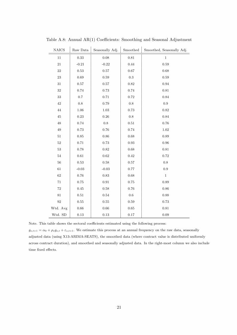
Table A.8: Annual AR(1) Coefficients: Smoothing and Seasonal Adjustment

NAICS Raw Data Seasonally Adj. Smoothed Smoothed, Seasonally Adj.

11 0.33 0.08 0.81 1

21 -0.21 -0.22 0.44 0.59

22 0.53 0.57 0.67 0.68

23 0.69 0.59 0.3 0.59

31 0.57 0.57 0.82 0.94

32 0.74 0.73 0.74 0.81

33 0.7 0.71 0.72 0.84

42 0.8 0.79 0.8 0.9

44 1.06 1.03 0.73 0.82

45 0.23 0.26 0.8 0.84

48 0.74 0.8 0.51 0.76

49 0.73 0.76 0.74 1.02

51 0.85 0.86 0.68 0.89

52 0.71 0.73 0.93 0.96

53 0.78 0.82 0.68 0.81

54 0.61 0.62 0.42 0.72

56 0.53 0.58 0.57 0.8

61 -0.03 -0.03 0.77 0.9

62 0.76 0.83 0.68 1

71 0.75 0.91 0.75 0.89

72 0.45 0.58 0.76 0.86

81 0.51 0.54 0.6 0.88

92 0.55 0.55 0.59 0.73

Wtd. Avg 0.66 0.66 0.65 0.81

Wtd. SD 0.13 0.13 0.17 0.09

Note. This table shows the sectoral coefficients estimated using the following process:

gs,t+1 = α0 + ρsgs,t + εs,t+1. We estimate this process at an annual frequency on the raw data, seasonally

adjusted data (using X13-ARIMA-SEATS), the smoothed data (where contract value is distributed uniformly

across contract duration), and smoothed and seasonally adjusted data. In the right-most column we also include

time fixed effects.

21

Table A.9: AR1 Persistence Estimates Across Frequencies

Monthly Quarterly Annual

Raw Data 0.42 0.46 0.78

Smooth, S.A. 0.94 0.94 0.82

Raw, Omit Top 1 Perc. 0.36 0.14 0.78

DOD: Raw Data 0.41 0.5 0.76

DOD: Smooth, S.A. 0.91 0.9 0.73

Non-DOD: Raw Data 0.41 0.31 0.8

Non-DOD: Smooth, S.A. 0.92 0.92 0.76

Note. This table shows the estimates of the AR(1) parameter in a simple first-order autoregressive specification

for sectoral government spending, at a monthly, quarterly and annual frequency. Rows denote different data

treatments, and subsets to DOD and non-DOD data. We estimate the process on the raw data, seasonally

adjusted (using X13-ARIMA-SEATS) and smoothed data (where contract value is distributed uniformly across

contract duration), and omitting the top 1% of contracts in value.

22

Table A.10: Distribution of Contract Pricing Types

All Contracts Top 10 Firms

Pricing Type Share (Count) Share (Value) Share (Count) Share (Value)

Combination 0.28 1.19 1.53 1.88

Cost No Fee 0.63 2.74 1.59 1.49

Cost Award Fee 0.94 11.52 6.44 17.38

Cost Fixed Fee 3.37 13.02 15.61 16.22

Cost Incentive 0.25 4.31 2.56 8.24

Cost Sharing 0.05 0.09 0.03 0.03

Firm Fixed Price 70.54 48.77 47.93 33.99

Fixed Price 1.09 1.85 1.06 2.65

Fixed Price Award 0.11 0.4 0.39 0.52

Fixed Price Incentive 0.22 4.56 2.72 12.53

Fixed Price Level of Effort 0.07 0.19 0.13 0.2

Fixed Price Redetermination 0.19 0.16 0.32 0.15

Fixed Price Economic Adj. 13.27 5.02 10.24 1.48

Labor Hours 1.19 1.18 1.23 0.42

Order Dependent 0.41 0.04 0.34 0.02

Time and Materials 2.28 3.6 5.66 2.13

Other or Not Reported 5.12 1.37 2.1 0.61

Total Fixed Price Contracts 85.49 60.95 62.79 51.52

Note. This table shows the shares by count and value of contracts by pricing type for all firms and for the top

10 firms. As a whole, most contracts are “Fixed Price”, but the distribution differs slightly for the top 10 firms

where a larger share are “Cost Fixed Fee.”

23

Table A.11: Estimated AR(1) at the Sectoral Level

(Monthly) No Time Fixed Effects

Sector ρ σ2 Θ

11 0.4168 0.441 0.458

21 0.1961 0.667 0.2877

22 0.383 0.203 0.3997

23 0.2306 0.434 0.2552

31 0.2068 0.152 0.216

32 0.252 0.678 0.1714

33 0.4604 0.167 0.1207

42 0.6646 0.2 0.3039

44 0.4738 0.283 0.2288

45 0.5794 0.512 0.1851

48 0.6652 0.237 0.3487

49 0.508 0.515 0.1697

51 0.4148 0.211 0.1345

52 0.3081 1.14 0.1935

53 0.0959 0.89 0.1927

54 0.4474 0.153 0.0697

55 0.0486 1.82 NA

56 0.4058 0.169 0.1389

61 0.2701 0.255 0.0552

62 0.5137 0.446 0.0741

71 0.3192 0.322 0.0498

72 0.446 0.274 0.2388

81 0.329 0.149 0.0464

92 0.3568 0.443 NA

Average 0.4236 0.2457 0.1367

(Monthly) Time Fixed Effects

Sector ρ σ2 Θ

11 0.2751 0.324 0.458

21 0.1734 0.57 0.2877

22 0.4478 0.124 0.3997

23 0.0406 0.235 0.2552

31 -0.0261 0.0965 0.216

32 0.1877 0.509 0.1714

33 0.3004 0.12 0.1207

42 0.577 0.131 0.3039

44 0.4638 0.203 0.2288

45 0.5347 0.406 0.1851

48 0.6341 0.173 0.3487

49 0.4562 0.368 0.1697

51 0.2738 0.0847 0.1345

52 0.3163 0.961 0.1935

53 0.142 0.765 0.1927

54 0.2434 0.056 0.0697

55 0.0667 1.72 NA

56 0.3896 0.0934 0.1389

61 0.2563 0.192 0.0552

62 0.546 0.306 0.0741

71 0.3233 0.27 0.0498

72 0.4571 0.178 0.2388

81 0.2007 0.104 0.0464

92 0.4379 0.405 NA

Average 0.2864 0.1562 0.1367

Note. The tables above show the coefficients, ρ, the variance terms σ2, and the price-stickiness terms for each

two-digit NAICS sector. ρ and σ2 are estimated using equation A.29 at a monthly frequency for government

contract obligations, without time fixed effects in the left table and with time fixed effects in the right table.

24

Table A.12: Estimated AR(1) at the Sectoral Level

(Quarterly) No Time Fixed Effects

Sector ρ σ2 Θ

11 -0.0204 0.387 0.458

21 -0.0307 0.595 0.2877

22 0.1966 0.112 0.3997

23 -0.0298 0.37 0.2552

31 0.4364 0.07 0.216

32 0.6218 0.175 0.1714

33 0.6509 0.0772 0.1207

42 0.7988 0.0966 0.3039

44 0.5985 0.162 0.2288

45 0.4496 0.615 0.1851

48 0.654 0.175 0.3487

49 0.6746 0.255 0.1697

51 0.5141 0.111 0.1345

52 0.4103 0.759 0.1935

53 0.7821 0.186 0.1927

54 0.3261 0.107 0.0697

55 -0.029 2 NA

56 0.3917 0.0822 0.1389

61 -0.08 0.206 0.0552

62 0.5196 0.292 0.0741

71 0.4375 0.191 0.0498

72 0.3039 0.183 0.2388

81 0.344 0.0675 0.0464

92 0.3523 0.277 NA

Average 0.4548 0.1416 0.1367

(Quarterly) Time Fixed Effects

Sector ρ σ2 Θ

11 -0.111 0.261 0.458

21 -0.0574 0.518 0.2877

22 0.2529 0.067 0.3997

23 -0.1163 0.198 0.2552

31 0.3364 0.0282 0.216

32 0.5399 0.19 0.1714

33 0.5926 0.0545 0.1207

42 0.6701 0.0837 0.3039

44 0.585 0.107 0.2288

45 0.4445 0.471 0.1851

48 0.6714 0.151 0.3487

49 0.673 0.167 0.1697

51 0.3972 0.0523 0.1345

52 0.449 0.722 0.1935

53 0.6954 0.204 0.1927

54 0.2675 0.0472 0.0697

55 -0.0126 1.79 NA

56 0.3538 0.0624 0.1389

61 0.0947 0.183 0.0552

62 0.5425 0.233 0.0741

71 0.5407 0.162 0.0498

72 0.3813 0.128 0.2388

81 0.2154 0.0422 0.0464

92 0.4278 0.27 NA

Average 0.4007 0.0968 0.1367

Note. The tables above show the coefficients, ρ, the variance terms σ2, and the price-stickiness terms for each

two-digit NAICS sector. ρ and σ2 are estimated using equation A.29 at a quarterly frequency for government

contract obligations, without time fixed effects in the left table and with time fixed effects in the right table.

25

A.4 What are Government Contracts?

Figure A.9: Tracing of Award from Origin to Recipient

Parent Award Agency

Awarding Agency

AwardingSub-Agency

Award Recipient Parent

Recipient 1

Recipient 2NAICS 1

NAICS 2

Product/Service 1

Product/Service 2

Zip Code 1 Zip Code 2

Funding Agency

Government Side Firm Side

A.4.1 Types of Awards

The government can use different types of awards to procure services. The majority of federal

spending through contracts is done through either a definitive contract action (DCA) or a

delivery order. A DCA is a legally binding agreement obligating the seller to furnish certain

supplies or services and the buyer to pay for them. For example, on April 27, 2018, Lockheed

Martin was awarded an $828,724,214 contract to build guided multiple launch rocket systems

for the Department of the Army. Funds for the project were obligated at the time of the award,

and the expected time of completion is September 2021.

A delivery order, on the other hand, is a contract that does not specify a firm quantity, but

provides issuance of orders for the delivery of goods or services during the period of the contract.

For example, on January 21, 2015, a company called Ace Maintenance & Services, Inc. was

awarded a $13,663,688 contract for janitorial services at Naval Support Activity Bethesda. The

work to be performed under the contract included all labor, supervision, management, tools,

materials, equipment, facilities, incidental engineering, and other items necessary to provide

26

janitorial services. The initial contract action was for a base period of one year and one month,

with the option of four additional years. The contract stipulated a maximum dollar amount for

the base period and four option years of $69,698,540. DCAs tend to be used for larger, one-time

purchases, while delivery orders are used for smaller and more frequent purchases.

Figure A.24 shows the share of each type of award by count and value for all firms (top

two panels) and the top 10 firms (bottom two panels). By count, delivery orders and purchase

orders are the most common type of award. By value, however, definitive contract actions

account for about half of the dollars spent. This is even more the case when looking solely at

the top 10 firms. This makes perfect sense, as delivery orders are usually used for smaller, more

frequent purchases (think of opening a “tab” with a company for supplies or services), while

definitive contract actions are used for large one-time purchases. As shown in Figure A.24,

there was a notable jump in the number of delivery orders in fiscal year 2015, largely explained

by two indefinite delivery vehicle contracts that were awarded, respectively, to the Lockheed

Martin Corporation and the Sikorsky Aircraft Corporation. The Lockheed Martin Corporation

contract was for “miscellaneous fire control equipment,” and comprised almost 50,000 individual

transactions in fiscal year 2015 for small items like a “switch, toggle” or “padlock.” Similarly, the

Sikorsky Aircraft Corporation contract for “airframe structural components” comprised around

13,000 individual transactions. By nature, these delivery order transactions are small in value,

which is why we see only an increase in the delivery order count, but not a large increase in the

share of delivery orders by value.3

3Sikorsky PIID: SPE4AX14D9421; Lockheed Martin PIID: SPE7L114D0002

27

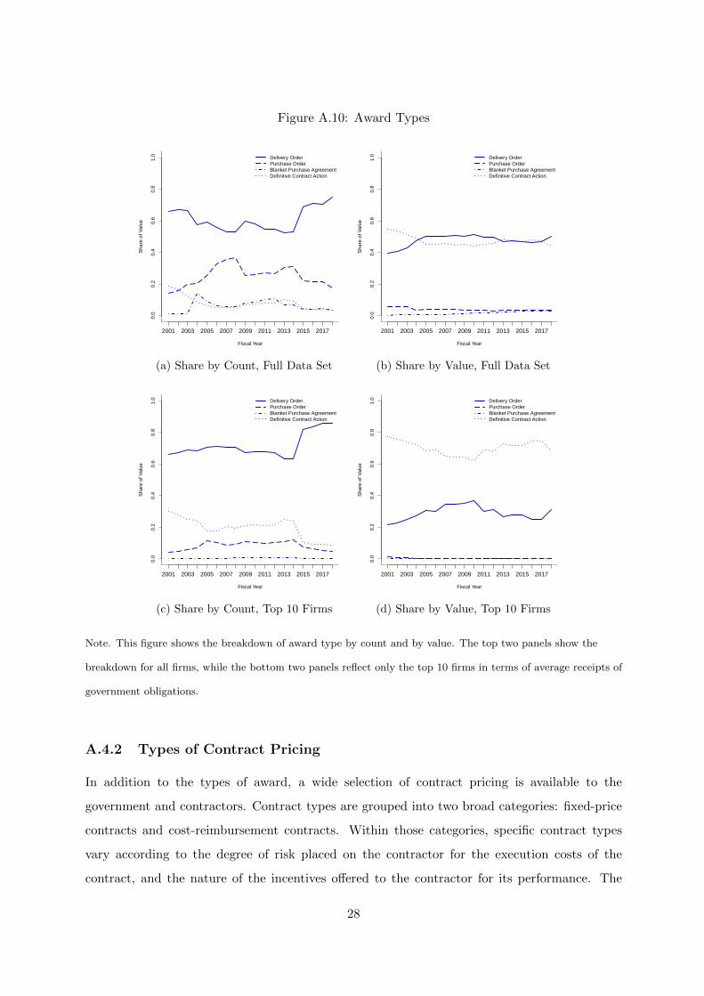
Figure A.10: Award Types

0.0

0.2

0.4

0.6

0.8

1.0

Fiscal Year

Sha

re o

f Val

ue

Delivery OrderPurchase OrderBlanket Purchase AgreementDefinitive Contract Action

2001 2003 2005 2007 2009 2011 2013 2015 2017

(a) Share by Count, Full Data Set0.

00.

20.

40.

60.

81.

0

Fiscal Year

Sha

re o

f Val

ue

Delivery OrderPurchase OrderBlanket Purchase AgreementDefinitive Contract Action

2001 2003 2005 2007 2009 2011 2013 2015 2017

(b) Share by Value, Full Data Set

0.0

0.2

0.4

0.6

0.8

1.0

Fiscal Year

Sha

re o

f Val

ue

Delivery OrderPurchase OrderBlanket Purchase AgreementDefinitive Contract Action

2001 2003 2005 2007 2009 2011 2013 2015 2017

(c) Share by Count, Top 10 Firms

0.0

0.2

0.4

0.6

0.8

1.0

Fiscal Year

Sha

re o

f Val

ue

Delivery OrderPurchase OrderBlanket Purchase AgreementDefinitive Contract Action

2001 2003 2005 2007 2009 2011 2013 2015 2017

(d) Share by Value, Top 10 Firms

Note. This figure shows the breakdown of award type by count and by value. The top two panels show the

breakdown for all firms, while the bottom two panels reflect only the top 10 firms in terms of average receipts of

government obligations.

A.4.2 Types of Contract Pricing

In addition to the types of award, a wide selection of contract pricing is available to the

government and contractors. Contract types are grouped into two broad categories: fixed-price

contracts and cost-reimbursement contracts. Within those categories, specific contract types

vary according to the degree of risk placed on the contractor for the execution costs of the

contract, and the nature of the incentives offered to the contractor for its performance. The

28

most common type of contract is a firm-fixed-price contract, which details a price that is not

subject to any adjustment, regardless of the contractor’s actual cost experience in executing the

contract. Fixed-price contracts can also include provisions for economic adjustment or incentive

payments, somewhat reducing the risk placed on the contractor.

Cost-reimbursement contracts are also frequent, and typically include a negotiated fixed fee

or an award amount on top of the reimbursement payment. We discuss in further detail what

the data on contract pricing look like when we discuss our fifth fact in the next section.

The pricing structure of a contract depends on many factors: price competition, the

complexity and urgency of the requirement, and the length of the contract, to name a few.

Many contracts are complex and require hybrid pricing structures. The multiple launch rocket

system contract mentioned above, for example, is a “cost-plus-fixed-fee, firm-fixed-price, and

fixed-price-incentive” hybrid. According to the FAR, “the objective is to negotiate a contract

type and price (or estimated cost and fee) that will result in reasonable contractor risk and

provide the contractor with the greatest incentive for efficient and economical performance.”

A.4.3 Competition

Federal regulations generally require contracting officers to promote full and open competition in

soliciting offers and awarding government contracts. In most cases, agencies are directed to use

sealed bids, competitive proposals, or some combination of competitive procedures to solicit and

issue awards. Ultimately, about half of the awarded contracts were fully and openly competitive

via negotiated proposals. The Ace Maintenance & Services, Inc. contract for janitorial services,

for example, was solicited using the Navy Electronic Commerce Online website, and seven

proposals were received.

A number of cases, however, exist, in which full and open competition is not required. Some

contracts are deemed “not available for competition,” in which case agencies are authorized

by statute to solicit bids from only one source. Solicitation from one source is authorized

if, for example, the supplies or services required by the agency are available from only one

responsible source or, for the Department of Defense, NASA, and the Coast Guard, from only

one or a limited number of responsible sources. Supplies can also be deemed available from

only the original source if the contract is a follow-on to an existing contract for the continued

development or production of a major system or highly specialized equipment. The Lockheed

Martin contract for guided multiple launch rocket systems is an example of the latter. Finally,

29

for smaller awards—those below a certain dollar threshold—federal agencies are required to

use “Simplified Acquisition Procedures (SAPs),” which reduce administrative costs, increase

efficiency, and improve opportunities for small and minority-owned businesses.

A.4.4 Extent Competed

By law — the Competition in Contracting Act (CICA) of 1984 (41 U.S.C. 253)—the government

is required to provide for full and open competition through the use of competitive procedures or

a combination of competitive procedures best suited to the circumstances of the contract action.

There are only a limited number of exceptions to this rule in which agencies can be given

authorization to use single-source or limited competition. For smaller awards—those below a

certain dollar threshold—federal agencies are required to use “Simplified Acquisition Procedures

(SAPs).” These procedures are typically used for the purchase of commonly purchased supplies

or services such as office supplies, computer software, and groundskeeping services. SAPs

reduce administrative costs, improve opportunities for small and minority-owned businesses,

and increase efficiency. The SAP threshold is $150,000, though this can vary by situation.4

There is a lower bound to the threshold also—$3,000—below which a purchase is considered a

“micro purchase,’ and different acquisition procedures apply.

Figure A.25 shows that both for all firms and for the top 10 firms, about half of transactions

are awarded under “full and open competition” (which includes “competitive delivery orders”).

This is true both by count and by value of transaction. By value, slightly more of the contracts

awarded to the top 10 firms are non-competitive, and, in particular, are “not available for

competition.” This is no surprise, given that the top 10 firms include places like Lockheed Martin

and General Dynamics—companies that are building specialized equipment for the military and

are often the sole source of a given product. Similar to what we saw in section ??, there is a sharp

increase in the number of full and open competition transactions to the top 10 firms around

2015. The transactions comprising the large indefinite delivery vehicle contracts discussed in

Section ?? were all deemed to be under full and open competition, helping to explain the increase.

4For example, for supplies or services supporting a contingency operation or facilitating defense against orrecovery from nuclear, biological, chemical, or radiological attack, the simplified acquisition threshold is $300,000for contracts awarded and performed or purchases made inside the US and $1 million for contracts awarded andperformed or purchases made outside the US

30

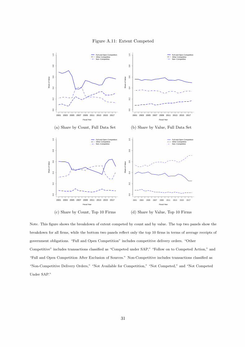
Figure A.11: Extent Competed

0.0

0.2

0.4

0.6

0.8

1.0

Fiscal Year

Sha

re o

f Val

ue

Full and Open CompetitionOther CompetitiveNon−Competitive

2001 2003 2005 2007 2009 2011 2013 2015 2017

(a) Share by Count, Full Data Set0.

00.

20.

40.

60.

81.

0

Fiscal Year

Sha

re o

f Val

ue

Full and Open CompetitionOther CompetitiveNon−Competitive

2001 2003 2005 2007 2009 2011 2013 2015 2017

(b) Share by Value, Full Data Set

0.0

0.2

0.4

0.6

0.8

1.0

Fiscal Year

Sha

re o

f Val

ue

Full and Open CompetitionOther CompetitiveNon−Competitive

2001 2003 2005 2007 2009 2011 2013 2015 2017

(c) Share by Count, Top 10 Firms

0.0

0.2

0.4

0.6

0.8

1.0

Fiscal Year

Sha

re o

f Val

ue

Full and Open CompetitionOther CompetitiveNon−Competitive

2001 2003 2005 2007 2009 2011 2013 2015 2017

(d) Share by Value, Top 10 Firms

Note. This figure shows the breakdown of extent competed by count and by value. The top two panels show the

breakdown for all firms, while the bottom two panels reflect only the top 10 firms in terms of average receipts of

government obligations. “Full and Open Competition” includes competitive delivery orders. “Other

Competitive” includes transactions classified as “Competed under SAP,” “Follow on to Competed Action,” and

“Full and Open Competition After Exclusion of Sources.” Non-Competitive includes transactions classified as

“Non-Competitive Delivery Orders,” “Not Available for Competition,” “Not Competed,” and “Not Competed

Under SAP.”

31

A.4.5 Who Gets the Longest Contracts?

The transactions/contracts with the longest durations go to just a handful of recipients. It

appears that many of these longer-term contracts have to do with facilities maintenance and

investment around the government. The recipients of the 30 transactions with the longest

durations include:

• Johnson Controls Inc. (14) – the recipient with the longest-duration contracts, by far, is an

HVAC company that provides services to federal buildings across the government

• United Technologies (2) – primarily an aircraft manufacturing company

• URS Corporation (2) – Now AECOM, an engineering, design and construction firm.

Provides services like hazardous waste treatment and disposal, engineering services,’and

facilities support services

• Gentex (2) – a company that develops electronic products for the automotive, aerospace, and

fire protection industries. Supplies things like specialized clothing, aircraft manufacturing

and other miscellaneous manufacturing

• Ameresco Inc (2) – an energy efficiency and energy infrastructure company that has

contracts with a number of agenices for energy efficieny and performance and energy

infrastructure projects

• State of Texas (2) – has received contracts from a multitude of agencies for a wide range of

services like food services, fossil fuel electric power generation, data processing, janitorial

services, etc.

The sectoral composition of long- and short-duration transactions differs as well.

• Of long transactions – those with durations that exceed three years – 70 percent of

the transactions are in NAICS 51 (Information) and NAICS 54 (Professional, Scientific,

and Technical Services). NAICS 33 (Manufacturing) and NAICS 56 (Administrative and

Support and Waste Management and Remediation Services) round out the top four recipient

sectors for long transactions

• Of “short” transactions – those with durations below three years – 70 percent of

transactions are in NAICS 33 (Manufacturing) and NAICS 42 (Wholesale Trade). NAICS

54 (Professional, Scientific, and Technical Services) and NAICS 23 (Construction) round

out the top four recipient sectors for short transactions.

32

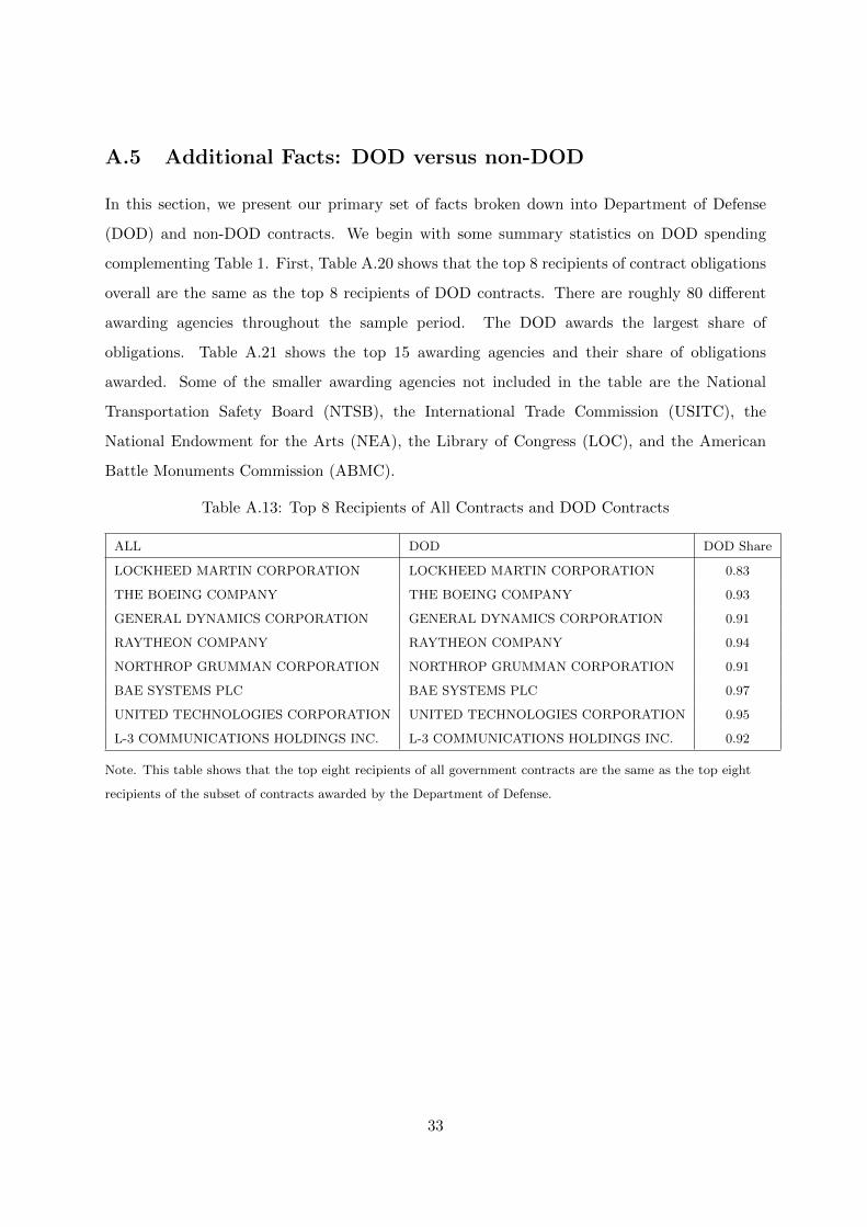
A.5 Additional Facts: DOD versus non-DOD

In this section, we present our primary set of facts broken down into Department of Defense

(DOD) and non-DOD contracts. We begin with some summary statistics on DOD spending

complementing Table 1. First, Table A.20 shows that the top 8 recipients of contract obligations

overall are the same as the top 8 recipients of DOD contracts. There are roughly 80 different

awarding agencies throughout the sample period. The DOD awards the largest share of

obligations. Table A.21 shows the top 15 awarding agencies and their share of obligations

awarded. Some of the smaller awarding agencies not included in the table are the National

Transportation Safety Board (NTSB), the International Trade Commission (USITC), the

National Endowment for the Arts (NEA), the Library of Congress (LOC), and the American

Battle Monuments Commission (ABMC).

Table A.13: Top 8 Recipients of All Contracts and DOD Contracts

ALL DOD DOD Share

LOCKHEED MARTIN CORPORATION LOCKHEED MARTIN CORPORATION 0.83

THE BOEING COMPANY THE BOEING COMPANY 0.93

GENERAL DYNAMICS CORPORATION GENERAL DYNAMICS CORPORATION 0.91

RAYTHEON COMPANY RAYTHEON COMPANY 0.94

NORTHROP GRUMMAN CORPORATION NORTHROP GRUMMAN CORPORATION 0.91

BAE SYSTEMS PLC BAE SYSTEMS PLC 0.97

UNITED TECHNOLOGIES CORPORATION UNITED TECHNOLOGIES CORPORATION 0.95

L-3 COMMUNICATIONS HOLDINGS INC. L-3 COMMUNICATIONS HOLDINGS INC. 0.92

Note. This table shows that the top eight recipients of all government contracts are the same as the top eight

recipients of the subset of contracts awarded by the Department of Defense.

33

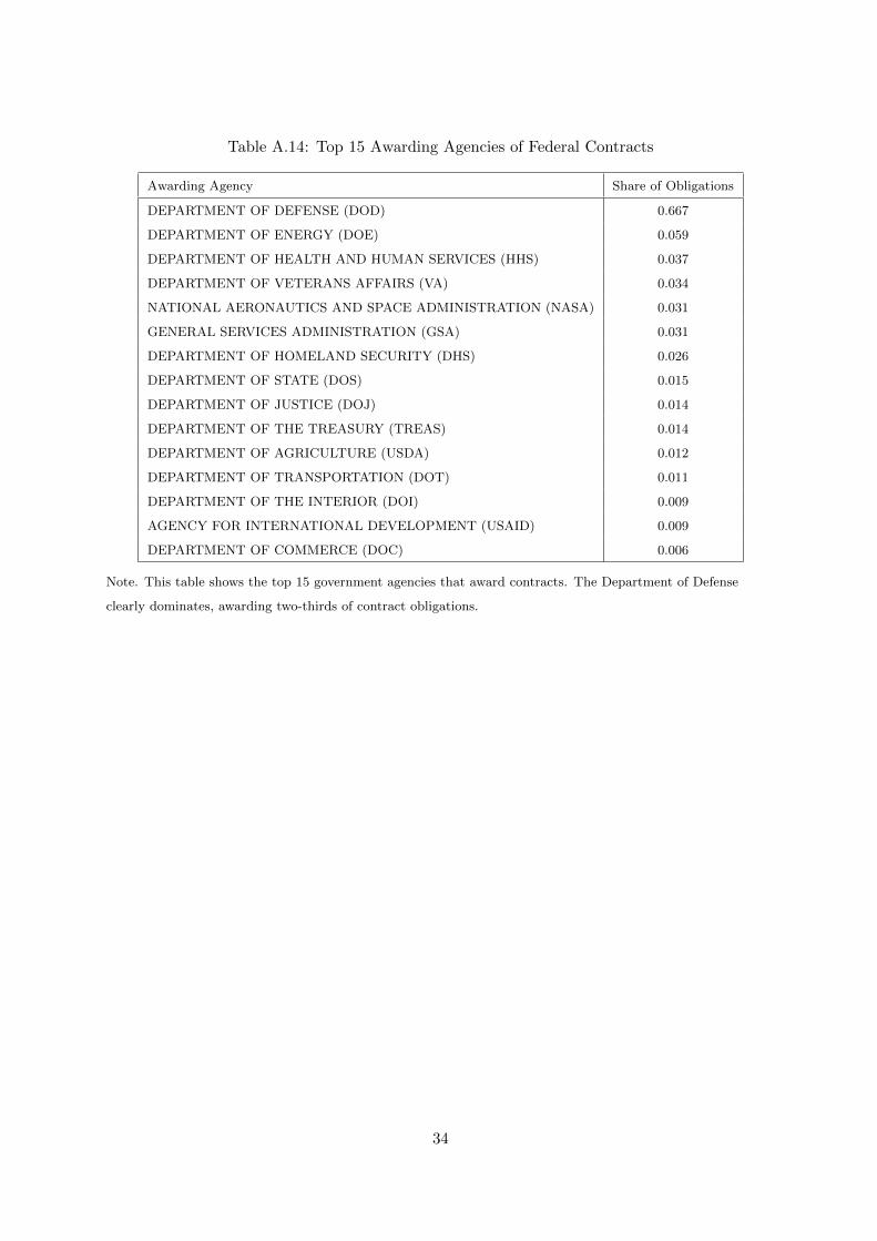
Table A.14: Top 15 Awarding Agencies of Federal Contracts

Awarding Agency Share of Obligations

DEPARTMENT OF DEFENSE (DOD) 0.667

DEPARTMENT OF ENERGY (DOE) 0.059

DEPARTMENT OF HEALTH AND HUMAN SERVICES (HHS) 0.037

DEPARTMENT OF VETERANS AFFAIRS (VA) 0.034

NATIONAL AERONAUTICS AND SPACE ADMINISTRATION (NASA) 0.031

GENERAL SERVICES ADMINISTRATION (GSA) 0.031

DEPARTMENT OF HOMELAND SECURITY (DHS) 0.026

DEPARTMENT OF STATE (DOS) 0.015

DEPARTMENT OF JUSTICE (DOJ) 0.014

DEPARTMENT OF THE TREASURY (TREAS) 0.014

DEPARTMENT OF AGRICULTURE (USDA) 0.012

DEPARTMENT OF TRANSPORTATION (DOT) 0.011

DEPARTMENT OF THE INTERIOR (DOI) 0.009

AGENCY FOR INTERNATIONAL DEVELOPMENT (USAID) 0.009

DEPARTMENT OF COMMERCE (DOC) 0.006

Note. This table shows the top 15 government agencies that award contracts. The Department of Defense

clearly dominates, awarding two-thirds of contract obligations.

34

Figure A.12: Share of Obligations by Top Firms and Sectors

0.0

0.2

0.4

0.6

0.8

1.0

Sha

re o

f Tot

al C

ontr

act V

alue ●

●●●

●●●●●●●●

●●●●

●●●●●

●●●●●●●●●●●●

●●●●●●●●●●●●●●●●●●●●●●●●●

●●●●●●●●●●●●●●●●●●●●●●●●●●●●●●●●●●●●●●●●●

●●●●●●●●●●●●●●●●●●●●●●●●●●●●●●●●●●●●●●●

●●●●●●●●●●●●●

●●●●●●●

●●●●●●●●●●●●●●●●●●●●●●●●●●●●●●●●●

●●●●●●●●●●●●●

●●●

2001 2003 2005 2007 2009 2011 2013 2015 2017

●

Top 10 FirmsTop 0.1 PercentTop 1 PercentTop 10 Percent

(a) Firms (ALL)

0.0

0.2

0.4

0.6

0.8

1.0

Sha

re o

f Tot

al C

ontr

act V

alue ●

●●●

●●●

●●●●●

●●●●

●●●●●

●●●●●●

●●●●●●

●●●●●●●●●●

●●●●●●●●●●●●●●●●●●●●

●●●●●●●●●

●●●●●●●●●●●●●●●●●●●●●●●●●●●●●●●●●●●●●●●●●●●●●●●●●●●●●●●●●●●●●●●●●●

●●●●●●●●●●

●●●●●●●●●●

●●●●●●●

●●●●●●●●●●●●●●●●●●●●●●●●●●●●●●●

●●●●●●●●●●

●

2001 2003 2005 2007 2009 2011 2013 2015 2017

●

Top 10 FirmsTop 0.1 PercentTop 1 PercentTop 10 Percent

(b) Firms (DOD)

0.0

0.2

0.4

0.6

0.8

1.0

Sha

re o

f Tot

al C

ontr

act V

alue

●

●●●

●●●

●●●●●●●●●●

●●●

●●●●●●●●●

●●●●●●

●●●●●●●●●●●●●●

●●●●●●●●●

●●●

●●●●●

●●●●

●●●●●●●

●●●●●●●●●●●●●●●●

●●●●●●●

●●●●●

●

●●●●●●●●●●●

●●●●●●●●●

●●●●●

●●●●●●●

●●●●●●●●●●●●●

●●●●●●●●●●●

●●●●●●●●●●●●●

●●●●●●●●●●●●●

●●●●●●●●●

●●●●●●●●●●

2001 2003 2005 2007 2009 2011 2013 2015 2017

●

Top 10 FirmsTop 0.1 PercentTop 1 PercentTop 10 Percent

(c) Firms (Non-DOD)

0.0

0.2

0.4

0.6

0.8

1.0

Sha

re o

f Tot

al C

ontr

act V

alue

●●●●●●●●●●●●●●●●●●●●●●●●●●●●●●●●●

●●●●●●●●●●●●

●●●●●●●

●●●●●●●●●●●

●

●

●●●●●●●●●●●●●●●●●●●●●●●●●●●●●●●●●●●●●●●●●●●●●●●●●●●●●●●●●●●●●●●●●●●●●●●●●●●●●●●●●●●●●●●●●●●●●●●●●●●●●●●●●●●●●●●●●●●●●●●●●●●●●●●●●●●●●●●●●●●●●●

2001 2003 2005 2007 2009 2011 2013 2015 2017

●

Top 5 SectorsTop 1 PercentTop 10 Percent

(d) NAICS 6 (ALL)

0.0

0.2

0.4

0.6

0.8

1.0

Sha

re o

f Tot

al C

ontr

act V

alue

●●●●●●●●●●●●●

●●●●●

●●●●●●●●●●●●●

●●●●●●●●

●●●●●●

●●●●

●●●

●●●●●●●●●●●

●

●

●●●●●●●●●●●●●●●●●●●●●●●●●●●●●●●●●●●●●●●●●●●●●●●●●●●●●●●●●●●●●●●●●●●●●●●●●●●●●●●●●●●●●●●●●●●●●●●●●●●●●●●●●●●●●●●●●●●●●●●●●●●●●●●●●●●●●●●●●●●●●●

2001 2003 2005 2007 2009 2011 2013 2015 2017

●

Top 5 SectorsTop 1 PercentTop 10 Percent

(e) NAICS 6 (DOD)

0.0

0.2

0.4

0.6

0.8

1.0

Sha

re o

f Tot

al C

ontr

act V

alue

●●●●●●●

●●●●●●●●●●●●●●●●●●●●

●●●●●●●●●●●

●

●●●●●●●●●●●●●●●●●●●

●●●●●●●●●●●●●●●●●

●●●●●●●●●●●●●●●●●●●●●●●●●●●●●●●

●●●●●●●●●●●●●●●●●●●●●●●●●●●●●●●●●●●●●●●●●●●●●●●●●●●●●●●●●●●●●●●●●●●●●●●●●●●●●●●●●●●●

●●●●●●●●●●●●●●●●●

2001 2003 2005 2007 2009 2011 2013 2015 2017

●

Top 5 SectorsTop 1 PercentTop 10 Percent

(f) NAICS 6 (Non-DOD)

0.0

0.2

0.4

0.6

0.8

1.0

Sha

re o

f Tot

al C

ontr

act V

alue

●●●●●●

●●●●●●●●●●●●●●

●●●●●●●●●●●●●●●●●●●●●●●●●●●●●●●●●●●●●●●●●●●●●●●●●●●●●●●●●●●●●●●●●●●●●●●●●●●●●●●

●●●●●●●●●●●●●●●●●●●

●●●●●●●●●●●●●●●●●●●●●●●●●●●●●●●

●●●●●●●●●●●●●●●●●●●●●●●●●●●●●●●●●●●●●●●●●●●●●●●●●●●●●●●●●●

2001 2003 2005 2007 2009 2011 2013 2015 2017

●

Top 1 SectorTop 2Top 5Top 10

(g) NAICS 2 (ALL)

0.0

0.2

0.4

0.6

0.8

1.0

Sha

re o

f Tot

al C

ontr

act V

alue

●●●●

●●

●●●●●●●

●●●●●

●●●●●●

●●●●●●●●●

●●●●

●●●●●●●●●●●●●

●●●●●●●●●●●●●

●

●●●●●

●●●●●

●●●●●

●●●●●●●●●●●●●●●●●

●●●●●●

●●●●●●●●●●●●●●●●●●●●●●●●●●●●●●●

●●●●

●●●●●

●●●●

●●●●●●

●●●●●●●●

●●●●●●●●

●●●●●●●●●●●●●●●●●●●●●●●

●●●●●●

●●●●●●●●●●

2001 2003 2005 2007 2009 2011 2013 2015 2017

●

Top 1 SectorTop 2Top 5Top 10

(h) NAICS 2 (DOD)

0.0

0.2

0.4

0.6

0.8

1.0

Sha

re o

f Tot

al C

ontr

act V

alue

●●●●●●●

●●●●

●●●●●●●

●●●●●●●●●

●●●●●●●●●●●●

●●●●●●●●●●●●●

●●●●●●●●●●●

●●●●●●●●●●●●

●●●●●●

●●●●●●●●●

●●●●●●●●●

●●●

●●●●●●●●●

●

●●●●●●●●●●●●●●

●●●●●●●●●

●●●●●●●●●●●●●●●●

●●●●●●●●●●●●●●●●●●●●●●●●●●●●●●●●●●

●●●●●●●●●●●

●●●

●●●●●●●●

2001 2003 2005 2007 2009 2011 2013 2015 2017

●

Top 1 SectorTop 2Top 5Top 10

(i) NAICS 2 (Non-DOD)

Note. This figure shows the share of contract obligations given to the top shares of firms (the left panel),

six-digit NAICS sectors (the middle panel), and two-digit NAICS sectors (the bottom panel).

35

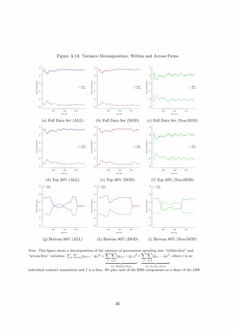
Figure A.13: Variance Decomposition: Within and Across Firms

2005 2010 2015

0.0

0.2

0.4

0.6

0.8

1.0

Fiscal Year

Sha

re o

f Tot

al V

aria

nce

WithinAcross

(a) Full Data Set (ALL)

2005 2010 2015

0.0

0.2

0.4

0.6

0.8

1.0

Fiscal Year

Sha

re o

f Tot

al V

aria

nce

WithinAcross

(b) Full Data Set (DOD)

2005 2010 2015

0.0

0.2

0.4

0.6

0.8

1.0

Fiscal Year

Sha

re o

f Tot

al V

aria

nce

WithinAcross

(c) Full Data Set (Non-DOD)

2005 2010 2015

0.0

0.2

0.4

0.6

0.8

1.0

Fiscal Year

Sha

re o

f Tot

al V

aria

nce

WithinAcross

(d) Top 20% (ALL)

2005 2010 2015

0.0

0.2

0.4

0.6

0.8

1.0

Fiscal Year

Sha

re o

f Tot

al V

aria

nce

WithinAcross

(e) Top 20% (DOD)

2005 2010 2015

0.0

0.2

0.4

0.6

0.8

1.0

Fiscal Year

Sha

re o

f Tot

al V

aria

nce

WithinAcross

(f) Top 20% (Non-DOD)

2005 2010 2015

0.0

0.2

0.4

0.6

0.8

1.0

Fiscal Year

Sha

re o

f Tot

al V

aria

nce

WithinAcross

(g) Bottom 80% (ALL)

2005 2010 2015

0.0

0.2

0.4

0.6

0.8

1.0

Fiscal Year

Sha

re o

f Tot

al V

aria

nce

WithinAcross

(h) Bottom 80% (DOD)

2005 2010 2015

0.0

0.2

0.4

0.6

0.8

1.0

Fiscal Year

Sha

re o

f Tot

al V

aria

nce

WithinAcross

(i) Bottom 80% (Non-DOD)

Note. This figure shows a decomposition of the variance of government spending into “within-firm” and

“across-firm” variation:∑f

∑i∈f (gif,t − gt)

2 =∑f

∑i∈f

(gif,t − gf,t)2

︸ ︷︷ ︸(a) Within Firm

+∑f

∑i∈f

(gf,t − gt)2

︸ ︷︷ ︸(b) Across Firm

, where i is an

individual contract transaction and f is a firm. We plot each of the RHS components as a share of the LHS.

36

Figure A.14: Density of Variance Decomposition Components

−5 0 5 10 15 20 25

0.0

0.1

0.2

0.3

0.4

0.5

Den

sity Transactions

Avg. Firm ObligationsAvg. Monthly Obligations

(a) Full Data Set (ALL)

−5 0 5 10 15 20 25

0.0

0.1

0.2

0.3

0.4

0.5

Den

sity Transactions

Avg. Firm ObligationsAvg. Monthly Obligations

(b) Full Data Set (DOD)

−5 0 5 10 15 20 25

0.0

0.1

0.2

0.3

0.4

0.5

Den

sity Transactions

Avg. Firm ObligationsAvg. Monthly Obligations

(c) Full Data Set (Non-DOD)

10 15 20 25

0.0

0.1

0.2

0.3

0.4

0.5

Den

sity Transactions

Avg. Firm ObligationsAvg. Monthly Obligations

(d) Top 20% (ALL)

10 15 20 25

0.0

0.1

0.2

0.3

0.4

0.5

Den

sity Transactions

Avg. Firm ObligationsAvg. Monthly Obligations

(e) Top 20% (DOD)

10 15 20

0.0

0.1

0.2

0.3

0.4

0.5

Den

sity Transactions

Avg. Firm ObligationsAvg. Monthly Obligations

(f) Top 20% (Non-DOD)

−5 0 5 10

0.0

0.1

0.2

0.3

0.4

0.5

Den

sity

TransactionsAvg. Firm ObligationsAvg. Monthly Obligations

(g) Bottom 80% (ALL)

−5 0 5 10

0.0

0.1

0.2

0.3

0.4

0.5

Den

sity

TransactionsAvg. Firm ObligationsAvg. Monthly Obligations

(h) Bottom 80% (DOD)

−5 0 5 10

0.0

0.1

0.2

0.3

0.4

0.5

Den

sity

TransactionsAvg. Firm ObligationsAvg. Monthly Obligations

(i) Bottom 80% (Non-DOD)

Note. This figure shows the density of each of the three components that underlie the variance decomposition in

Figure ??. The solid line shows the density of the individual contract transactions—gif,t; the dot-dash line

shows the density of average firm obligations—gf,t; and the dashed line shows the density of average annual

obligations—gt.

37

Figure A.15: Variance Decomposition: Within and Across Sectors

0.0

0.2

0.4

0.6

0.8

1.0

Fiscal Year

Sha

re o

f Tot

al V

aria

nce

2001 2003 2005 2007 2009 2011 2013 2015 2017

WithinAcross

(a) Full Dataset (ALL)

0.0

0.2

0.4

0.6

0.8

1.0

Fiscal Year

Sha

re o

f Tot

al V

aria

nce

2001 2003 2005 2007 2009 2011 2013 2015 2017

WithinAcross

(b) Full Dataset (DOD)

0.0

0.2

0.4

0.6

0.8

1.0

Fiscal Year

Sha

re o

f Tot

al V

aria

nce

2001 2003 2005 2007 2009 2011 2013 2015 2017

WithinAcross

(c) Full Dataset (Non-DOD)

0.0

0.2

0.4

0.6

0.8

1.0

Fiscal Year

Sha

re o

f Tot

al V

aria

nce

2001 2003 2005 2007 2009 2011 2013 2015 2017

WithinAcross

(d) Top 20% (ALL)

0.0

0.2

0.4

0.6

0.8

1.0

Fiscal Year

Sha

re o

f Tot

al V

aria

nce

2001 2003 2005 2007 2009 2011 2013 2015 2017

WithinAcross

(e) Top 20% (DOD)

0.0

0.2

0.4

0.6

0.8

1.0

Fiscal Year

Sha

re o

f Tot

al V

aria

nce

2001 2003 2005 2007 2009 2011 2013 2015 2017

WithinAcross

(f) Top 20% (Non-DOD)

0.0

0.2

0.4

0.6

0.8

1.0

Fiscal Year

Sha

re o

f Tot

al V

aria

nce

2001 2003 2005 2007 2009 2011 2013 2015 2017

WithinAcross

(g) Bottom 80% (ALL)

0.0

0.2

0.4

0.6

0.8

1.0

Fiscal Year

Sha

re o

f Tot

al V

aria

nce

2001 2003 2005 2007 2009 2011 2013 2015 2017

WithinAcross

(h) Bottom 80% (DOD)

0.0

0.2

0.4

0.6

0.8

1.0

Fiscal Year

Sha

re o

f Tot

al V

aria

nce

2001 2003 2005 2007 2009 2011 2013 2015 2017

WithinAcross

(i) Bottom 80% (Non-DOD)

Note. This figure shows a decomposition of the variance of government spending into “within-firm” and

“across-firm” variation:∑f

∑i∈f (gif,t − gt)

2 =∑f

∑i∈f

(gif,t − gf,t)2

︸ ︷︷ ︸(a) Within Firm

+∑f

∑i∈f

(gf,t − gt)2

︸ ︷︷ ︸(b) Across Firm

, where i is an

individual contract transaction and f is a firm. We plot each of the RHS components as a share of the LHS.

38

Figure A.16: Density of Sectoral Variance Decomposition Components

−5 0 5 10 15 20 25

0.0

0.1

0.2

0.3

0.4

0.5

Den

sity Transactions

Avg.Sector ObligationsAvg. Annual Obligations

(a) Full Dataset (ALL)

−5 0 5 10 15 20 25

0.0

0.1

0.2

0.3

0.4

0.5

Den

sity Transactions

Avg.Sector ObligationsAvg. Annual Obligations

(b) Full Dataset (DOD)

−5 0 5 10 15 20 25

0.0

0.1

0.2

0.3

0.4

0.5

Den

sity Transactions

Avg.Sector ObligationsAvg. Annual Obligations

(c) Full Dataset (DOD)

10 15 20 25

0.0

0.1

0.2

0.3

0.4

0.5

Den

sity Transactions

Avg.Sector ObligationsAvg. Annual Obligations

(d) Top 20% (ALL)

10 15 20 25

0.0

0.1

0.2

0.3

0.4

0.5

Den

sity Transactions

Avg.Sector ObligationsAvg. Annual Obligations

(e) Top 20% (DOD)

10 15 20

0.0

0.1

0.2

0.3

0.4

0.5

Den

sity Transactions

Avg.Sector ObligationsAvg. Annual Obligations

(f) Top 20% (DOD)

−5 0 5 10

0.0

0.2

0.4

0.6

0.8

Den

sity

TransactionsAvg.Sector ObligationsAvg. Annual Obligations

(g) Bottom 80% (ALL)

−5 0 5 10

0.0

0.2

0.4

0.6

0.8

Den

sity

TransactionsAvg.Sector ObligationsAvg. Annual Obligations

(h) Bottom 80% (DOD)

−5 0 5 10

0.0

0.2

0.4

0.6

0.8

Den

sity

TransactionsAvg.Sector ObligationsAvg. Annual Obligations

(i) Bottom 80% (DOD)

Note. This figure shows the density of each of the three components that underly the variance decomposition in

figure A.4. The solid line shows the density of the individual contract transactions—gif,t, the dot-dash line

shows the density of average firm obligations—gf,t, and the dashed line shows the density of average annual

obligations—gt.

39

Figure A.17: Q-Q Plot: Actual vs. Log-Normal

●

●

●●

●●

●●

●●

●●●●●●●●●●●●●●●●●●●

●●●●●●●

●●●●●●●

●●●●●●

●●●●●●

●●●●●●

●●●●●●

●●●●●

●●●●

●●●●

●●●●●●●

●●

●●

●●

●●

●

●

●

●

2 4 6 8 10 12 14

24

68

1012

14

Theoretical Quantiles

Act

ual Q

uant

iles

(a) All Contracts

●

●

●

●

●

●●●●●●●●●●●●●●●

●●●●●●

●●●●●●

●●●●●●

●●●●●●

●●●●●●

●●●●●

●●●●●

●●●●

●●●●

●●●●

●●●●

●●●●

●●●●●●

●●

●●

●●

●●

●

●

●

●

●

6 8 10 12 146

810

1214

Theoretical Quantiles

Act

ual Q

uant

iles

(b) DOD Contracts

●

●

●●

●●

●●

●●●●●●●

●●●●●●

●●●●

●●●●

●●●●

●●●●●●●●●●●●●

●●●●●●

●●●●●●

●●●●●

●●●●

●●●●

●●●●

●●●●

●●●●●●●

●●

●●

●●

●●

●

●

●

●

●

2 4 6 8 10 12 14

24

68

1012

14

Theoretical Quantiles

Act

ual Q

uant

iles

(c) Non-DOD Contracts

●

●

●

●●

●●●●●●●●●●●●●●●●

●●●●●

●●●●●

●●●●●●

●●●●●●

●●●●●●

●●●●●●

●●●●

●●●●

●●●●

●●●●

●●●●

●●●●

●●●●●●●●●

●●

●●

●●

●

●

●

●

●

6 8 10 12 14 16

68

1012

1416

18

Theoretical Quantiles

Act

ual Q

uant

iles

(d) All Firms

●

●●

●● ●●●●●●●●●●●●●●

●●●●

●●●●

●●●●

●●●●●

●●●●●

●●●●

●●●●●●●●●●

●●●●

●●●●

●●●●

●●●●

●●●●

●●●●●●●●●●●●●

●●

●●

●●

●

●

●

●

●

6 8 10 12 14 16 18

810

1214

1618

Theoretical Quantiles

Act

ual Q

uant

iles

(e) DOD Firms

●

●

●

●

●●

●●●●●●●●●●●●●

●●●●

●●●●●

●●●●●

●●●●●

●●●●●●

●●●●●●●●

●●●●●

●●●●

●●●●

●●●●

●●●●

●●●●

●●●●

●●●●●●●

●●

●●

●●

●

●

●

●

●

6 8 10 12 14 16

68

1012

1416

18

Theoretical Quantiles

Act

ual Q

uant

iles

(f) Non-DOD Firms

●

●

●●

●

●●

●●

●●

●●●

●●●●●●●

●●●●●

●●●●

●●●●●

●●●●

●●●●●

●●●●●

●●●●●

●●●●

●●●●

●●●●●

●●●●

●●●●●

●●●●

●●●●●●●●●●

●●

●●

●

●●

●

●

12 14 16 18 20 22 24 26

1214

1618

2022

2426

Theoretical Quantiles

Act

ual Q

uant

iles

(g) All Sectors

●

●

●

●

●●

●●

●●

●●●●●

●●●

●●●●

●●●●

●●●●

●●●●

●●●●

●●●●●

●●●●●●●●●

●●●●

●●●●●

●●●●

●●●●

●●●●●

●●●●

●●●●

●●●●●●●●●●

●●

●●

●

●

●

15 20 25

1015

2025

Theoretical Quantiles

Act

ual Q

uant

iles

(h) DOD Sectors

●

●

●

●

●

●●

●●●

●●●●●

●●●

●●●●

●●●●

●●●●

●●●●●●●

●●●●●

●●●●●

●●●●●●●

●●●●

●●●●

●●●●●●

●●●●

●●●●

●●●●

●●●●●●●

●●

●●

●●

●●

●●

●

●

12 14 16 18 20 22 24

1214

1618

2022

24

Theoretical Quantiles

Act

ual Q

uant

iles

(i) Non-DOD Sectors

Note. The figures above are Q-Q plots with actual quantiles of log transactions on the y-axis and theoretical

quantiles from a log-normal distribution with the same mean and standard deviation plotted on the x-axis.

That the points fall along the 45-degree line suggests that all three subsets of the data are well-approximated by

a log-normal distribution. Data represent a single annual cross section from the year 2012, but patterns are

robust in any year of the sample.

40

Figure A.18: Empirical CDF of Contract Durations

0.0

0.2

0.4

0.6

0.8

1.0

Duration (Days)

Cum

ulat

ive

Sha

re

0 1000 2000 3000 4000 5000 6000

ContractsMulti−Transaction Contracts

(a) DOD0.

00.

20.

40.

60.

81.

0

Duration (Days)

Cum

ulat

ive

Sha

re

0 1000 2000 3000 4000 5000 6000

ContractsMulti−Transaction Contracts

(b) Non-DOD

Note. This figure shows the empirical cumulative distribution function of the duration—the number of days

between the start and end-date—of transactions and contracts. The dashed black line marks 365 days.

Contracts with negative durations or durations more than 5500 days (15 years) are excluded. Transactions

represent the observation level of the data. Contracts are bundles of transactions that pertain to the same

award. Multi-Transaction Contracts are the subset of contracts that are made up of more than one transaction.

Figure A.19: Initial and Modification Spending

100

150

200

250

300

Fiscal Year

Bill

ion

Dol

lars

2001 2003 2005 2007 2009 2011 2013 2015 2017

(a) All

5010

015

020

0

Fiscal Year

Bill

ion

Dol

lars

2001 2003 2005 2007 2009 2011 2013 2015 2017

(b) DOD

050

100

150

Fiscal Year

Bill

ion

Dol

lars

2001 2003 2005 2007 2009 2011 2013 2015 2017

(c) Non-DOD

Note. This figure shows the levels of initial spending (any transaction that is not delineated a modification) and

modification spending (transactions that are classified as modifications).

41

Figure A.21: Decomposition of Sectoral Spending Growth−

0.4

−0.

20.

00.

20.

4

Fiscal Year

Per

cent

Cha

nge

●

●

●

●

●●

●

●

●

● ●

●

●

●

●

●

●

2002 2004 2006 2008 2010 2012 2014 2016 2018

●

AggregateEqual WeightsGranular ResidualShare Deviation

(a) All

−0.

20.

00.

20.

4

Fiscal Year

Per

cent

Cha

nge

●

●

●

●

●

●

●

●

●

●

●

●

●

●

●

●

●

2002 2004 2006 2008 2010 2012 2014 2016 2018

●

AggregateEqual WeightsGranular ResidualShare Deviation

(b) DOD

−0.

20.

00.

20.

4

Fiscal Year

Per

cent

Cha

nge

●

●

●

●

●

●

●

●

●

●

●

●●

●

●

●

2002 2004 2006 2008 2010 2012 2014 2016 2018

●

AggregateEqual WeightsGranular ResidualShare Deviation

(c) Non-DOD

Note. This figure plots the individual components of government consumption growth, decomposed as inFoerster et al. (2011) as follows:

Zt =N∑i=1

ωi,tzi,t︸ ︷︷ ︸(1) Actual

=1

N

N∑i=1

zi,t︸ ︷︷ ︸(2) Equal Weights

+N∑i=1

(ωi −

1

N

)zi,t︸ ︷︷ ︸

(3) Granular Residual

+N∑i=1

(ωi,t − ωi)zi,t︸ ︷︷ ︸(4) Share Deviation

Figure A.20: Density of Error Term Correlation Coefficients

−0.4 −0.2 0.0 0.2 0.4 0.6

0.0

0.5

1.0

1.5

2.0

2.5

Den

sity

(a) All Contracts

−0.4 −0.2 0.0 0.2 0.4 0.6

0.0

0.5

1.0

1.5

2.0

2.5

Den

sity

(b) DOD Contracts

−0.4 −0.2 0.0 0.2 0.4

0.0

0.5

1.0

1.5

2.0

2.5

Den

sity

(c) NON-DOD Contracts

Note. This figure shows the distribution of correlation across sector pairs that result from examining the

sectoral process: gs,t+1 = α0 + αs + αt + ρsgs,t + εs,t+1, where gs,t is the log of government consumption of

output from two-digit sector s in year t. The figure shows the distribution of the correlation coefficients of the

residuals for all sector pairs.

42

Figure A.22: Sectoral Spending and Price Rigidity

0.00 0.05 0.10 0.15 0.20 0.25 0.30

0.0

0.1

0.2

0.3

0.4

0.5

Share of Spending

Fre

quen

cy o

f Pric

e C

hang

es

●

●

●

●

●

●

●

●

●

●

●

●

●●

●

●

●

●

●

●

(a) All (BLS)

0.0 0.1 0.2 0.3 0.4

0.0

0.1

0.2

0.3

0.4

0.5

Share of Spending

Fre

quen

cy o

f Pric

e C

hang

es

●

●

●

●

●

●

●

●

●

●

●

●

●●

●

●

●

●

●

●

(b) DOD (BLS)

0.0 0.1 0.2 0.3 0.4

0.0

0.1

0.2

0.3

0.4

0.5

Share of SpendingF

requ

ency

of P

rice

Cha

nges

●

●

●

●

●

●

●

●

●

●

●

●

●

● ●

●

●

●

●

●

(c) Non-DOD (BLS)

0.00 0.05 0.10 0.15 0.20 0.25 0.30

0.0

0.2

0.4

0.6

0.8

Share of Spending

Fre

quen

cy o

f Pric

e C

hang

es

●

●

●

●

● ●

●

●

●

●

●

●

●

●

●●

●

●

●

●

●

●

(d) All (Duration)

0.0 0.1 0.2 0.3 0.4

0.0

0.2

0.4

0.6

0.8

1.0

Share of Spending

Fre

quen

cy o

f Pric

e C

hang

es

●

●

●

●

●

●●

●

●

●

●

●

●

● ●●

●

●

●

●

●

●

(e) DOD (Duration)

0.0 0.1 0.2 0.3 0.4

0.0

0.2

0.4

0.6

0.8

1.0

Share of Spending

Fre

quen

cy o

f Pric

e C

hang

es

●

●

●

●

●

●

●

●

●

●

●

●

●

●

●

●●

●

●

●

●

●

(f) Non-DOD (Duration)

Note. This figure shows the average annual share of government spending in each two-digit sector (x-axis)

plotted against the frequency of price changes in those sectors, based on BLS data, in the top row, and based on

the inverse sectoral contract duration in the bottom row. The size of the bubble corresponds with the average

sectoral share of annual aggregate spending.

43

Tables A.22 and A.23 show regressions of aggregate defense and non-defense government

spending on the firm-level granular residual and its lags for DOD and non-DOD contracts,

respectively. Tables A.24 and A.25 show regressions of aggregate defense and non-defense

government spending, respectively, on the sector-level granular residual. All specifications show

that the granular residual is an important determinant of variation in government spending

growth.

Table A.15: Explanatory Power of the Granular Residual (Firms)

(1) (2)∆G ∆G

ΓQ=5000t 0.831∗∗∗ 0.808∗∗∗

(0.0691) (0.0696)

ΓQ=5000t−1 0.174∗

(0.0709)

ΓQ=5000t−2 -0.0324

(0.0678)Constant 0.236∗∗∗ 0.251∗∗∗

(0.0185) (0.0228)

Observations 201 199R2 0.421 0.461

Standard errors in parentheses∗ p < 0.05, ∗∗ p < 0.01, ∗∗∗ p < 0.001

Table A.16: Explanatory Power of the Granular Residual (Firms)

(1) (2)∆G ∆G

ΓQ=5000t 0.660∗∗∗ 0.644∗∗∗

(0.0873) (0.0864)

ΓQ=5000t−1 0.130

(0.0863)

ΓQ=5000t−2 0.0145

(0.0865)Constant 0.217∗∗∗ 0.234∗∗∗

(0.0258) (0.0319)

Observations 201 199R2 0.223 0.233

Standard errors in parentheses∗ p < 0.05, ∗∗ p < 0.01, ∗∗∗ p < 0.001

44

Table A.17: Explanatory Power of the Granular Residual (Sectors)

(1) (2)∆G ∆G

ΓQ=1000t 0.820∗∗∗ 0.956∗∗∗

(0.0911) (0.0916)

ΓQ=1000t−1 0.0939

(0.0929)

ΓQ=1000t−2 -0.161

(0.0849)Constant 0.125∗∗∗ 0.119∗∗∗

(0.0158) (0.0153)

Observations 201 199R2 0.289 0.383

Standard errors in parentheses∗ p < 0.05, ∗∗ p < 0.01, ∗∗∗ p < 0.001

Table A.18: Explanatory Power of the Granular Residual (Sectors)

(1) (2)∆G ∆G

ΓQ=1000t 0.984∗∗∗ 0.935∗∗∗

(0.0984) (0.100)

ΓQ=1000t−1 0.138

(0.103)

ΓQ=1000t−2 -0.00609

(0.100)Constant 0.174∗∗∗ 0.176∗∗∗

(0.0209) (0.0221)

Observations 201 199R2 0.334 0.342

Standard errors in parentheses∗ p < 0.05, ∗∗ p < 0.01, ∗∗∗ p < 0.001

45

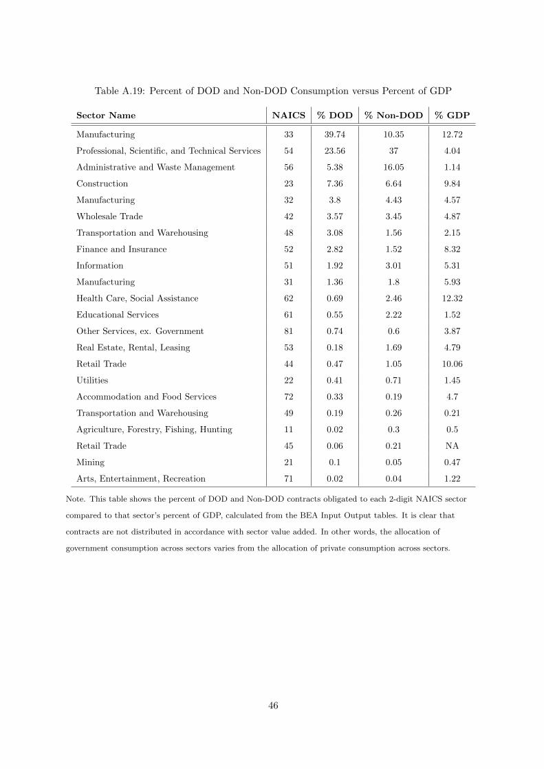
Table A.19: Percent of DOD and Non-DOD Consumption versus Percent of GDP

Sector Name NAICS % DOD % Non-DOD % GDP

Manufacturing 33 39.74 10.35 12.72

Professional, Scientific, and Technical Services 54 23.56 37 4.04

Administrative and Waste Management 56 5.38 16.05 1.14

Construction 23 7.36 6.64 9.84

Manufacturing 32 3.8 4.43 4.57

Wholesale Trade 42 3.57 3.45 4.87

Transportation and Warehousing 48 3.08 1.56 2.15

Finance and Insurance 52 2.82 1.52 8.32

Information 51 1.92 3.01 5.31

Manufacturing 31 1.36 1.8 5.93

Health Care, Social Assistance 62 0.69 2.46 12.32

Educational Services 61 0.55 2.22 1.52

Other Services, ex. Government 81 0.74 0.6 3.87

Real Estate, Rental, Leasing 53 0.18 1.69 4.79

Retail Trade 44 0.47 1.05 10.06

Utilities 22 0.41 0.71 1.45

Accommodation and Food Services 72 0.33 0.19 4.7

Transportation and Warehousing 49 0.19 0.26 0.21

Agriculture, Forestry, Fishing, Hunting 11 0.02 0.3 0.5

Retail Trade 45 0.06 0.21 NA

Mining 21 0.1 0.05 0.47

Arts, Entertainment, Recreation 71 0.02 0.04 1.22

Note. This table shows the percent of DOD and Non-DOD contracts obligated to each 2-digit NAICS sector

compared to that sector’s percent of GDP, calculated from the BEA Input Output tables. It is clear that

contracts are not distributed in accordance with sector value added. In other words, the allocation of

government consumption across sectors varies from the allocation of private consumption across sectors.

46

Supplemental Material:

Big G

Lydia Cox, Gernot J. Muller, Ernesto Pasten, Raphael Schoenle, and Michael Weber

Not for Publication

A.6 What are Government Contracts?

Figure A.23: Tracing of Award from Origin to Recipient

Parent Award Agency

Awarding Agency

AwardingSub-Agency

Award Recipient Parent

Recipient 1

Recipient 2NAICS 1

NAICS 2

Product/Service 1

Product/Service 2

Zip Code 1 Zip Code 2

Funding Agency

Government Side Firm Side

A.6.1 Types of Awards

The government can use different types of awards to procure services. The majority of federal

spending through contracts is done through either a definitive contract action (DCA) or a

delivery order. A DCA is a legally binding agreement obligating the seller to furnish certain

supplies or services and the buyer to pay for them. For example, on April 27, 2018, Lockheed

Martin was awarded an $828,724,214 contract to build guided multiple launch rocket systems

for the Department of the Army. Funds for the project were obligated at the time of the award,

and the expected time of completion is September 2021.

1

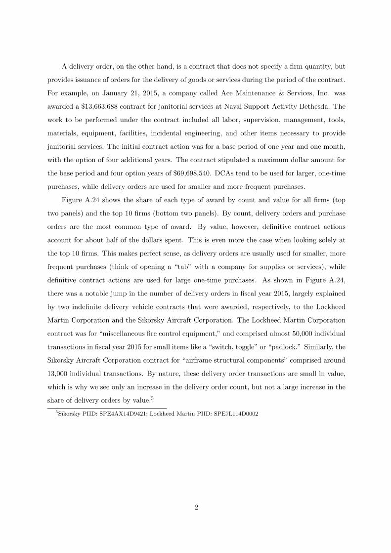
A delivery order, on the other hand, is a contract that does not specify a firm quantity, but

provides issuance of orders for the delivery of goods or services during the period of the contract.

For example, on January 21, 2015, a company called Ace Maintenance & Services, Inc. was

awarded a $13,663,688 contract for janitorial services at Naval Support Activity Bethesda. The

work to be performed under the contract included all labor, supervision, management, tools,

materials, equipment, facilities, incidental engineering, and other items necessary to provide

janitorial services. The initial contract action was for a base period of one year and one month,

with the option of four additional years. The contract stipulated a maximum dollar amount for

the base period and four option years of $69,698,540. DCAs tend to be used for larger, one-time

purchases, while delivery orders are used for smaller and more frequent purchases.

Figure A.24 shows the share of each type of award by count and value for all firms (top

two panels) and the top 10 firms (bottom two panels). By count, delivery orders and purchase

orders are the most common type of award. By value, however, definitive contract actions

account for about half of the dollars spent. This is even more the case when looking solely at

the top 10 firms. This makes perfect sense, as delivery orders are usually used for smaller, more

frequent purchases (think of opening a “tab” with a company for supplies or services), while

definitive contract actions are used for large one-time purchases. As shown in Figure A.24,

there was a notable jump in the number of delivery orders in fiscal year 2015, largely explained

by two indefinite delivery vehicle contracts that were awarded, respectively, to the Lockheed

Martin Corporation and the Sikorsky Aircraft Corporation. The Lockheed Martin Corporation

contract was for “miscellaneous fire control equipment,” and comprised almost 50,000 individual

transactions in fiscal year 2015 for small items like a “switch, toggle” or “padlock.” Similarly, the

Sikorsky Aircraft Corporation contract for “airframe structural components” comprised around

13,000 individual transactions. By nature, these delivery order transactions are small in value,

which is why we see only an increase in the delivery order count, but not a large increase in the

share of delivery orders by value.5

5Sikorsky PIID: SPE4AX14D9421; Lockheed Martin PIID: SPE7L114D0002

2

Figure A.24: Award Types

0.0

0.2

0.4

0.6

0.8

1.0

Fiscal Year

Sha

re o

f Val

ue

Delivery OrderPurchase OrderBlanket Purchase AgreementDefinitive Contract Action

2001 2003 2005 2007 2009 2011 2013 2015 2017

(a) Share by Count, Full Data Set0.

00.

20.

40.

60.

81.

0

Fiscal Year

Sha

re o

f Val

ue

Delivery OrderPurchase OrderBlanket Purchase AgreementDefinitive Contract Action

2001 2003 2005 2007 2009 2011 2013 2015 2017

(b) Share by Value, Full Data Set

0.0

0.2

0.4

0.6

0.8

1.0

Fiscal Year

Sha

re o

f Val

ue

Delivery OrderPurchase OrderBlanket Purchase AgreementDefinitive Contract Action

2001 2003 2005 2007 2009 2011 2013 2015 2017

(c) Share by Count, Top 10 Firms

0.0

0.2

0.4

0.6

0.8

1.0

Fiscal Year

Sha

re o

f Val

ue

Delivery OrderPurchase OrderBlanket Purchase AgreementDefinitive Contract Action

2001 2003 2005 2007 2009 2011 2013 2015 2017

(d) Share by Value, Top 10 Firms

Note. This figure shows the breakdown of award type by count and by value. The top two panels show the

breakdown for all firms, while the bottom two panels reflect only the top 10 firms in terms of average receipts of

government obligations.

A.6.2 Types of Contract Pricing

In addition to the types of award, a wide selection of contract pricing is available to the

government and contractors. Contract types are grouped into two broad categories: fixed-price

contracts and cost-reimbursement contracts. Within those categories, specific contract types

vary according to the degree of risk placed on the contractor for the execution costs of the

contract, and the nature of the incentives offered to the contractor for its performance. The

3

most common type of contract is a firm-fixed-price contract, which details a price that is not

subject to any adjustment, regardless of the contractor’s actual cost experience in executing the

contract. Fixed-price contracts can also include provisions for economic adjustment or incentive

payments, somewhat reducing the risk placed on the contractor.

Cost-reimbursement contracts are also frequent, and typically include a negotiated fixed fee

or an award amount on top of the reimbursement payment. We discuss in further detail what

the data on contract pricing look like when we discuss our fifth fact in the next section.

The pricing structure of a contract depends on many factors: price competition, the

complexity and urgency of the requirement, and the length of the contract, to name a few.

Many contracts are complex and require hybrid pricing structures. The multiple launch rocket

system contract mentioned above, for example, is a “cost-plus-fixed-fee, firm-fixed-price, and

fixed-price-incentive” hybrid. According to the FAR, “the objective is to negotiate a contract

type and price (or estimated cost and fee) that will result in reasonable contractor risk and

provide the contractor with the greatest incentive for efficient and economical performance.”

A.6.3 Competition

Federal regulations generally require contracting officers to promote full and open competition in

soliciting offers and awarding government contracts. In most cases, agencies are directed to use

sealed bids, competitive proposals, or some combination of competitive procedures to solicit and

issue awards. Ultimately, about half of the awarded contracts were fully and openly competitive

via negotiated proposals. The Ace Maintenance & Services, Inc. contract for janitorial services,

for example, was solicited using the Navy Electronic Commerce Online website, and seven

proposals were received.

A number of cases, however, exist, in which full and open competition is not required. Some

contracts are deemed “not available for competition,” in which case agencies are authorized

by statute to solicit bids from only one source. Solicitation from one source is authorized

if, for example, the supplies or services required by the agency are available from only one

responsible source or, for the Department of Defense, NASA, and the Coast Guard, from only

one or a limited number of responsible sources. Supplies can also be deemed available from

only the original source if the contract is a follow-on to an existing contract for the continued

development or production of a major system or highly specialized equipment. The Lockheed

Martin contract for guided multiple launch rocket systems is an example of the latter. Finally,

4

for smaller awards—those below a certain dollar threshold—federal agencies are required to

use “Simplified Acquisition Procedures (SAPs),” which reduce administrative costs, increase

efficiency, and improve opportunities for small and minority-owned businesses.

A.6.4 Extent Competed

By law — the Competition in Contracting Act (CICA) of 1984 (41 U.S.C. 253)—the government

is required to provide for full and open competition through the use of competitive procedures or

a combination of competitive procedures best suited to the circumstances of the contract action.

There are only a limited number of exceptions to this rule in which agencies can be given

authorization to use single-source or limited competition. For smaller awards—those below a

certain dollar threshold—federal agencies are required to use “Simplified Acquisition Procedures

(SAPs).” These procedures are typically used for the purchase of commonly purchased supplies

or services such as office supplies, computer software, and groundskeeping services. SAPs

reduce administrative costs, improve opportunities for small and minority-owned businesses,

and increase efficiency. The SAP threshold is $150,000, though this can vary by situation.6

There is a lower bound to the threshold also—$3,000—below which a purchase is considered a

“micro purchase,’ and different acquisition procedures apply.

Figure A.25 shows that both for all firms and for the top 10 firms, about half of transactions

are awarded under “full and open competition” (which includes “competitive delivery orders”).

This is true both by count and by value of transaction. By value, slightly more of the contracts

awarded to the top 10 firms are non-competitive, and, in particular, are “not available for

competition.” This is no surprise, given that the top 10 firms include places like Lockheed Martin

and General Dynamics—companies that are building specialized equipment for the military and

are often the sole source of a given product. Similar to what we saw in section ??, there is a sharp

increase in the number of full and open competition transactions to the top 10 firms around

2015. The transactions comprising the large indefinite delivery vehicle contracts discussed in

Section ?? were all deemed to be under full and open competition, helping to explain the increase.

6For example, for supplies or services supporting a contingency operation or facilitating defense against orrecovery from nuclear, biological, chemical, or radiological attack, the simplified acquisition threshold is $300,000for contracts awarded and performed or purchases made inside the US and $1 million for contracts awarded andperformed or purchases made outside the US

5

Figure A.25: Extent Competed

0.0

0.2

0.4

0.6

0.8

1.0

Fiscal Year

Sha

re o

f Val

ue

Full and Open CompetitionOther CompetitiveNon−Competitive

2001 2003 2005 2007 2009 2011 2013 2015 2017

(a) Share by Count, Full Data Set0.

00.

20.

40.

60.

81.

0

Fiscal Year

Sha

re o

f Val

ue

Full and Open CompetitionOther CompetitiveNon−Competitive

2001 2003 2005 2007 2009 2011 2013 2015 2017

(b) Share by Value, Full Data Set

0.0

0.2

0.4

0.6

0.8

1.0

Fiscal Year

Sha

re o

f Val

ue

Full and Open CompetitionOther CompetitiveNon−Competitive

2001 2003 2005 2007 2009 2011 2013 2015 2017

(c) Share by Count, Top 10 Firms

0.0

0.2

0.4

0.6

0.8

1.0

Fiscal Year

Sha

re o

f Val

ue

Full and Open CompetitionOther CompetitiveNon−Competitive

2001 2003 2005 2007 2009 2011 2013 2015 2017

(d) Share by Value, Top 10 Firms

Note. This figure shows the breakdown of extent competed by count and by value. The top two panels show the

breakdown for all firms, while the bottom two panels reflect only the top 10 firms in terms of average receipts of

government obligations. “Full and Open Competition” includes competitive delivery orders. “Other

Competitive” includes transactions classified as “Competed under SAP,” “Follow on to Competed Action,” and

“Full and Open Competition After Exclusion of Sources.” Non-Competitive includes transactions classified as

“Non-Competitive Delivery Orders,” “Not Available for Competition,” “Not Competed,” and “Not Competed

Under SAP.”

6

A.6.5 Who Gets the Longest Contracts?

The transactions/contracts with the longest durations go to just a handful of recipients. It

appears that many of these longer-term contracts have to do with facilities maintenance and

investment around the government. The recipients of the 30 transactions with the longest

durations include:

• Johnson Controls Inc. (14) – the recipient with the longest-duration contracts, by far, is an

HVAC company that provides services to federal buildings across the government

• United Technologies (2) – primarily an aircraft manufacturing company

• URS Corporation (2) – Now AECOM, an engineering, design and construction firm.

Provides services like hazardous waste treatment and disposal, engineering services,’and

facilities support services

• Gentex (2) – a company that develops electronic products for the automotive, aerospace, and

fire protection industries. Supplies things like specialized clothing, aircraft manufacturing

and other miscellaneous manufacturing

• Ameresco Inc (2) – an energy efficiency and energy infrastructure company that has

contracts with a number of agenices for energy efficieny and performance and energy

infrastructure projects

• State of Texas (2) – has received contracts from a multitude of agencies for a wide range of

services like food services, fossil fuel electric power generation, data processing, janitorial

services, etc.

The sectoral composition of long- and short-duration transactions differs as well.

• Of long transactions – those with durations that exceed three years – 70 percent of

the transactions are in NAICS 51 (Information) and NAICS 54 (Professional, Scientific,

and Technical Services). NAICS 33 (Manufacturing) and NAICS 56 (Administrative and

Support and Waste Management and Remediation Services) round out the top four recipient

sectors for long transactions

• Of “short” transactions – those with durations below three years – 70 percent of

transactions are in NAICS 33 (Manufacturing) and NAICS 42 (Wholesale Trade). NAICS

54 (Professional, Scientific, and Technical Services) and NAICS 23 (Construction) round

out the top four recipient sectors for short transactions.

7

A.7 Additional Facts: DOD versus non-DOD

In this section, we present our primary set of facts broken down into Department of Defense

(DOD) and non-DOD contracts. We begin with some summary statistics on DOD spending

complementing Table 1. First, Table A.20 shows that the top 8 recipients of contract obligations

overall are the same as the top 8 recipients of DOD contracts. There are roughly 80 different

awarding agencies throughout the sample period. The DOD awards the largest share of

obligations. Table A.21 shows the top 15 awarding agencies and their share of obligations

awarded. Some of the smaller awarding agencies not included in the table are the National

Transportation Safety Board (NTSB), the International Trade Commission (USITC), the

National Endowment for the Arts (NEA), the Library of Congress (LOC), and the American

Battle Monuments Commission (ABMC).

Table A.20: Top 8 Recipients of All Contracts and DOD Contracts

ALL DOD DOD Share

LOCKHEED MARTIN CORPORATION LOCKHEED MARTIN CORPORATION 0.83

THE BOEING COMPANY THE BOEING COMPANY 0.93

GENERAL DYNAMICS CORPORATION GENERAL DYNAMICS CORPORATION 0.91

RAYTHEON COMPANY RAYTHEON COMPANY 0.94

NORTHROP GRUMMAN CORPORATION NORTHROP GRUMMAN CORPORATION 0.91

BAE SYSTEMS PLC BAE SYSTEMS PLC 0.97

UNITED TECHNOLOGIES CORPORATION UNITED TECHNOLOGIES CORPORATION 0.95

L-3 COMMUNICATIONS HOLDINGS INC. L-3 COMMUNICATIONS HOLDINGS INC. 0.92

Note. This table shows that the top eight recipients of all government contracts are the same as the top eight

recipients of the subset of contracts awarded by the Department of Defense.

8

Table A.21: Top 15 Awarding Agencies of Federal Contracts

Awarding Agency Share of Obligations

DEPARTMENT OF DEFENSE (DOD) 0.667

DEPARTMENT OF ENERGY (DOE) 0.059

DEPARTMENT OF HEALTH AND HUMAN SERVICES (HHS) 0.037

DEPARTMENT OF VETERANS AFFAIRS (VA) 0.034

NATIONAL AERONAUTICS AND SPACE ADMINISTRATION (NASA) 0.031

GENERAL SERVICES ADMINISTRATION (GSA) 0.031

DEPARTMENT OF HOMELAND SECURITY (DHS) 0.026

DEPARTMENT OF STATE (DOS) 0.015

DEPARTMENT OF JUSTICE (DOJ) 0.014

DEPARTMENT OF THE TREASURY (TREAS) 0.014

DEPARTMENT OF AGRICULTURE (USDA) 0.012

DEPARTMENT OF TRANSPORTATION (DOT) 0.011

DEPARTMENT OF THE INTERIOR (DOI) 0.009

AGENCY FOR INTERNATIONAL DEVELOPMENT (USAID) 0.009

DEPARTMENT OF COMMERCE (DOC) 0.006

Note. This table shows the top 15 government agencies that award contracts. The Department of Defense

clearly dominates, awarding two-thirds of contract obligations.

9

Figure A.26: Share of Obligations by Top Firms and Sectors

0.0

0.2

0.4

0.6

0.8

1.0

Sha

re o

f Tot

al C

ontr

act V

alue ●

●●●

●●●●●●●●

●●●●

●●●●●

●●●●●●●●●●●●

●●●●●●●●●●●●●●●●●●●●●●●●●

●●●●●●●●●●●●●●●●●●●●●●●●●●●●●●●●●●●●●●●●●

●●●●●●●●●●●●●●●●●●●●●●●●●●●●●●●●●●●●●●●

●●●●●●●●●●●●●

●●●●●●●

●●●●●●●●●●●●●●●●●●●●●●●●●●●●●●●●●

●●●●●●●●●●●●●

●●●

2001 2003 2005 2007 2009 2011 2013 2015 2017

●

Top 10 FirmsTop 0.1 PercentTop 1 PercentTop 10 Percent

(a) Firms (ALL)

0.0

0.2

0.4

0.6

0.8

1.0

Sha

re o

f Tot

al C

ontr

act V

alue ●

●●●

●●●

●●●●●

●●●●

●●●●●

●●●●●●

●●●●●●

●●●●●●●●●●

●●●●●●●●●●●●●●●●●●●●

●●●●●●●●●

●●●●●●●●●●●●●●●●●●●●●●●●●●●●●●●●●●●●●●●●●●●●●●●●●●●●●●●●●●●●●●●●●●

●●●●●●●●●●

●●●●●●●●●●

●●●●●●●

●●●●●●●●●●●●●●●●●●●●●●●●●●●●●●●

●●●●●●●●●●

●

2001 2003 2005 2007 2009 2011 2013 2015 2017

●

Top 10 FirmsTop 0.1 PercentTop 1 PercentTop 10 Percent

(b) Firms (DOD)

0.0

0.2

0.4

0.6

0.8

1.0

Sha

re o

f Tot

al C

ontr

act V

alue

●

●●●

●●●

●●●●●●●●●●

●●●

●●●●●●●●●

●●●●●●

●●●●●●●●●●●●●●

●●●●●●●●●

●●●

●●●●●

●●●●

●●●●●●●

●●●●●●●●●●●●●●●●

●●●●●●●

●●●●●

●

●●●●●●●●●●●

●●●●●●●●●

●●●●●

●●●●●●●

●●●●●●●●●●●●●

●●●●●●●●●●●

●●●●●●●●●●●●●

●●●●●●●●●●●●●

●●●●●●●●●

●●●●●●●●●●

2001 2003 2005 2007 2009 2011 2013 2015 2017

●

Top 10 FirmsTop 0.1 PercentTop 1 PercentTop 10 Percent

(c) Firms (Non-DOD)

0.0

0.2

0.4

0.6

0.8

1.0

Sha

re o

f Tot

al C

ontr

act V

alue

●●●●●●●●●●●●●●●●●●●●●●●●●●●●●●●●●

●●●●●●●●●●●●

●●●●●●●

●●●●●●●●●●●

●

●

●●●●●●●●●●●●●●●●●●●●●●●●●●●●●●●●●●●●●●●●●●●●●●●●●●●●●●●●●●●●●●●●●●●●●●●●●●●●●●●●●●●●●●●●●●●●●●●●●●●●●●●●●●●●●●●●●●●●●●●●●●●●●●●●●●●●●●●●●●●●●●

2001 2003 2005 2007 2009 2011 2013 2015 2017

●

Top 5 SectorsTop 1 PercentTop 10 Percent

(d) NAICS 6 (ALL)

0.0

0.2

0.4

0.6

0.8

1.0

Sha

re o

f Tot

al C

ontr

act V

alue

●●●●●●●●●●●●●

●●●●●

●●●●●●●●●●●●●

●●●●●●●●

●●●●●●

●●●●

●●●

●●●●●●●●●●●

●

●

●●●●●●●●●●●●●●●●●●●●●●●●●●●●●●●●●●●●●●●●●●●●●●●●●●●●●●●●●●●●●●●●●●●●●●●●●●●●●●●●●●●●●●●●●●●●●●●●●●●●●●●●●●●●●●●●●●●●●●●●●●●●●●●●●●●●●●●●●●●●●●

2001 2003 2005 2007 2009 2011 2013 2015 2017

●

Top 5 SectorsTop 1 PercentTop 10 Percent

(e) NAICS 6 (DOD)

0.0

0.2

0.4

0.6

0.8

1.0

Sha

re o

f Tot

al C

ontr

act V

alue

●●●●●●●

●●●●●●●●●●●●●●●●●●●●

●●●●●●●●●●●

●

●●●●●●●●●●●●●●●●●●●

●●●●●●●●●●●●●●●●●

●●●●●●●●●●●●●●●●●●●●●●●●●●●●●●●

●●●●●●●●●●●●●●●●●●●●●●●●●●●●●●●●●●●●●●●●●●●●●●●●●●●●●●●●●●●●●●●●●●●●●●●●●●●●●●●●●●●●

●●●●●●●●●●●●●●●●●

2001 2003 2005 2007 2009 2011 2013 2015 2017

●

Top 5 SectorsTop 1 PercentTop 10 Percent

(f) NAICS 6 (Non-DOD)

0.0

0.2

0.4

0.6

0.8

1.0

Sha

re o

f Tot

al C

ontr

act V

alue

●●●●●●

●●●●●●●●●●●●●●

●●●●●●●●●●●●●●●●●●●●●●●●●●●●●●●●●●●●●●●●●●●●●●●●●●●●●●●●●●●●●●●●●●●●●●●●●●●●●●●

●●●●●●●●●●●●●●●●●●●

●●●●●●●●●●●●●●●●●●●●●●●●●●●●●●●

●●●●●●●●●●●●●●●●●●●●●●●●●●●●●●●●●●●●●●●●●●●●●●●●●●●●●●●●●●

2001 2003 2005 2007 2009 2011 2013 2015 2017

●

Top 1 SectorTop 2Top 5Top 10

(g) NAICS 2 (ALL)

0.0

0.2

0.4

0.6

0.8

1.0

Sha

re o

f Tot

al C

ontr

act V

alue

●●●●

●●

●●●●●●●

●●●●●

●●●●●●

●●●●●●●●●

●●●●

●●●●●●●●●●●●●

●●●●●●●●●●●●●

●

●●●●●

●●●●●

●●●●●

●●●●●●●●●●●●●●●●●

●●●●●●

●●●●●●●●●●●●●●●●●●●●●●●●●●●●●●●

●●●●

●●●●●

●●●●

●●●●●●

●●●●●●●●

●●●●●●●●

●●●●●●●●●●●●●●●●●●●●●●●

●●●●●●

●●●●●●●●●●

2001 2003 2005 2007 2009 2011 2013 2015 2017

●

Top 1 SectorTop 2Top 5Top 10

(h) NAICS 2 (DOD)

0.0

0.2

0.4

0.6

0.8

1.0

Sha

re o

f Tot

al C

ontr

act V

alue

●●●●●●●

●●●●

●●●●●●●

●●●●●●●●●

●●●●●●●●●●●●

●●●●●●●●●●●●●

●●●●●●●●●●●

●●●●●●●●●●●●

●●●●●●

●●●●●●●●●

●●●●●●●●●

●●●

●●●●●●●●●

●

●●●●●●●●●●●●●●

●●●●●●●●●

●●●●●●●●●●●●●●●●

●●●●●●●●●●●●●●●●●●●●●●●●●●●●●●●●●●

●●●●●●●●●●●

●●●

●●●●●●●●

2001 2003 2005 2007 2009 2011 2013 2015 2017

●

Top 1 SectorTop 2Top 5Top 10

(i) NAICS 2 (Non-DOD)

Note. This figure shows the share of contract obligations given to the top shares of firms (the left panel),

six-digit NAICS sectors (the middle panel), and two-digit NAICS sectors (the bottom panel).

10

Figure A.27: Variance Decomposition: Within and Across Firms

2005 2010 2015

0.0

0.2

0.4

0.6

0.8

1.0

Fiscal Year

Sha

re o

f Tot

al V

aria

nce

WithinAcross

(a) Full Data Set (ALL)

2005 2010 2015

0.0

0.2

0.4

0.6

0.8

1.0

Fiscal Year

Sha

re o

f Tot

al V

aria

nce

WithinAcross

(b) Full Data Set (DOD)

2005 2010 2015

0.0

0.2

0.4

0.6

0.8

1.0

Fiscal Year

Sha

re o

f Tot

al V

aria

nce

WithinAcross

(c) Full Data Set (Non-DOD)

2005 2010 2015

0.0

0.2

0.4

0.6

0.8

1.0

Fiscal Year

Sha

re o

f Tot

al V

aria

nce

WithinAcross

(d) Top 20% (ALL)

2005 2010 2015

0.0

0.2

0.4

0.6

0.8

1.0

Fiscal Year

Sha

re o

f Tot

al V

aria

nce

WithinAcross

(e) Top 20% (DOD)

2005 2010 2015

0.0

0.2

0.4

0.6

0.8

1.0

Fiscal Year

Sha

re o

f Tot

al V

aria

nce

WithinAcross

(f) Top 20% (Non-DOD)

2005 2010 2015

0.0

0.2

0.4

0.6

0.8

1.0

Fiscal Year

Sha

re o

f Tot

al V

aria

nce

WithinAcross

(g) Bottom 80% (ALL)

2005 2010 2015

0.0

0.2

0.4

0.6

0.8

1.0

Fiscal Year

Sha

re o

f Tot

al V

aria

nce

WithinAcross

(h) Bottom 80% (DOD)

2005 2010 2015

0.0

0.2

0.4

0.6

0.8

1.0

Fiscal Year

Sha

re o

f Tot

al V

aria

nce

WithinAcross

(i) Bottom 80% (Non-DOD)

Note. This figure shows a decomposition of the variance of government spending into “within-firm” and

“across-firm” variation:∑f

∑i∈f (gif,t − gt)

2 =∑f

∑i∈f

(gif,t − gf,t)2

︸ ︷︷ ︸(a) Within Firm

+∑f

∑i∈f

(gf,t − gt)2

︸ ︷︷ ︸(b) Across Firm

, where i is an

individual contract transaction and f is a firm. We plot each of the RHS components as a share of the LHS.

11

Figure A.28: Density of Variance Decomposition Components

−5 0 5 10 15 20 25

0.0

0.1

0.2

0.3

0.4

0.5

Den

sity Transactions

Avg. Firm ObligationsAvg. Monthly Obligations

(a) Full Data Set (ALL)

−5 0 5 10 15 20 25

0.0

0.1

0.2

0.3

0.4

0.5

Den

sity Transactions

Avg. Firm ObligationsAvg. Monthly Obligations

(b) Full Data Set (DOD)

−5 0 5 10 15 20 25

0.0

0.1

0.2

0.3

0.4

0.5

Den

sity Transactions

Avg. Firm ObligationsAvg. Monthly Obligations

(c) Full Data Set (Non-DOD)

10 15 20 25

0.0

0.1

0.2

0.3

0.4

0.5

Den

sity Transactions

Avg. Firm ObligationsAvg. Monthly Obligations

(d) Top 20% (ALL)

10 15 20 25

0.0

0.1

0.2

0.3

0.4

0.5

Den

sity Transactions

Avg. Firm ObligationsAvg. Monthly Obligations

(e) Top 20% (DOD)

10 15 20

0.0

0.1

0.2

0.3

0.4

0.5

Den

sity Transactions

Avg. Firm ObligationsAvg. Monthly Obligations

(f) Top 20% (Non-DOD)

−5 0 5 10

0.0

0.1

0.2

0.3

0.4

0.5

Den

sity

TransactionsAvg. Firm ObligationsAvg. Monthly Obligations

(g) Bottom 80% (ALL)

−5 0 5 10

0.0

0.1

0.2

0.3

0.4

0.5

Den

sity

TransactionsAvg. Firm ObligationsAvg. Monthly Obligations

(h) Bottom 80% (DOD)

−5 0 5 10

0.0

0.1

0.2

0.3

0.4

0.5

Den

sity

TransactionsAvg. Firm ObligationsAvg. Monthly Obligations

(i) Bottom 80% (Non-DOD)

Note. This figure shows the density of each of the three components that underlie the variance decomposition in

Figure ??. The solid line shows the density of the individual contract transactions—gif,t; the dot-dash line

shows the density of average firm obligations—gf,t; and the dashed line shows the density of average annual

obligations—gt.

12

Figure A.29: Variance Decomposition: Within and Across Sectors

0.0

0.2

0.4

0.6

0.8

1.0

Fiscal Year

Sha

re o

f Tot

al V

aria

nce

2001 2003 2005 2007 2009 2011 2013 2015 2017

WithinAcross

(a) Full Dataset (ALL)

0.0

0.2

0.4

0.6

0.8

1.0

Fiscal Year

Sha

re o

f Tot

al V

aria

nce

2001 2003 2005 2007 2009 2011 2013 2015 2017

WithinAcross

(b) Full Dataset (DOD)

0.0

0.2

0.4

0.6

0.8

1.0

Fiscal Year

Sha

re o

f Tot

al V

aria

nce

2001 2003 2005 2007 2009 2011 2013 2015 2017

WithinAcross

(c) Full Dataset (Non-DOD)

0.0

0.2

0.4

0.6

0.8

1.0

Fiscal Year

Sha

re o

f Tot

al V

aria

nce

2001 2003 2005 2007 2009 2011 2013 2015 2017

WithinAcross

(d) Top 20% (ALL)

0.0

0.2

0.4

0.6

0.8

1.0

Fiscal Year

Sha

re o

f Tot

al V

aria

nce

2001 2003 2005 2007 2009 2011 2013 2015 2017

WithinAcross

(e) Top 20% (DOD)

0.0

0.2

0.4

0.6

0.8

1.0

Fiscal Year

Sha

re o

f Tot

al V

aria

nce

2001 2003 2005 2007 2009 2011 2013 2015 2017

WithinAcross

(f) Top 20% (Non-DOD)

0.0

0.2

0.4

0.6

0.8

1.0

Fiscal Year

Sha

re o

f Tot

al V

aria

nce

2001 2003 2005 2007 2009 2011 2013 2015 2017

WithinAcross

(g) Bottom 80% (ALL)

0.0

0.2

0.4

0.6

0.8

1.0

Fiscal Year

Sha

re o

f Tot

al V

aria

nce

2001 2003 2005 2007 2009 2011 2013 2015 2017

WithinAcross

(h) Bottom 80% (DOD)

0.0

0.2

0.4

0.6

0.8

1.0

Fiscal Year

Sha

re o

f Tot

al V

aria

nce

2001 2003 2005 2007 2009 2011 2013 2015 2017

WithinAcross

(i) Bottom 80% (Non-DOD)

Note. This figure shows a decomposition of the variance of government spending into “within-firm” and

“across-firm” variation:∑f

∑i∈f (gif,t − gt)

2 =∑f

∑i∈f

(gif,t − gf,t)2

︸ ︷︷ ︸(a) Within Firm

+∑f

∑i∈f

(gf,t − gt)2

︸ ︷︷ ︸(b) Across Firm

, where i is an

individual contract transaction and f is a firm. We plot each of the RHS components as a share of the LHS.

13

Figure A.30: Density of Sectoral Variance Decomposition Components

−5 0 5 10 15 20 25

0.0

0.1

0.2

0.3

0.4

0.5

Den

sity Transactions

Avg.Sector ObligationsAvg. Annual Obligations

(a) Full Dataset (ALL)

−5 0 5 10 15 20 25

0.0

0.1

0.2

0.3

0.4

0.5

Den

sity Transactions

Avg.Sector ObligationsAvg. Annual Obligations

(b) Full Dataset (DOD)

−5 0 5 10 15 20 25

0.0

0.1

0.2

0.3

0.4

0.5

Den

sity Transactions

Avg.Sector ObligationsAvg. Annual Obligations

(c) Full Dataset (DOD)

10 15 20 25

0.0

0.1

0.2

0.3

0.4

0.5

Den

sity Transactions

Avg.Sector ObligationsAvg. Annual Obligations

(d) Top 20% (ALL)

10 15 20 25

0.0

0.1

0.2

0.3

0.4

0.5

Den

sity Transactions

Avg.Sector ObligationsAvg. Annual Obligations

(e) Top 20% (DOD)

10 15 20

0.0

0.1

0.2

0.3

0.4

0.5

Den

sity Transactions

Avg.Sector ObligationsAvg. Annual Obligations

(f) Top 20% (DOD)

−5 0 5 10

0.0

0.2

0.4

0.6

0.8

Den

sity

TransactionsAvg.Sector ObligationsAvg. Annual Obligations

(g) Bottom 80% (ALL)

−5 0 5 10

0.0

0.2

0.4

0.6

0.8

Den

sity

TransactionsAvg.Sector ObligationsAvg. Annual Obligations

(h) Bottom 80% (DOD)

−5 0 5 10

0.0

0.2

0.4

0.6

0.8

Den

sity

TransactionsAvg.Sector ObligationsAvg. Annual Obligations

(i) Bottom 80% (DOD)

Note. This figure shows the density of each of the three components that underly the variance decomposition in

figure A.4. The solid line shows the density of the individual contract transactions—gif,t, the dot-dash line

shows the density of average firm obligations—gf,t, and the dashed line shows the density of average annual

obligations—gt.

14

Figure A.31: Q-Q Plot: Actual vs. Log-Normal

●

●

●●

●●

●●

●●

●●●●●●●●●●●●●●●●●●●

●●●●●●●

●●●●●●●

●●●●●●

●●●●●●

●●●●●●

●●●●●●

●●●●●

●●●●

●●●●

●●●●●●●

●●

●●

●●

●●

●

●

●

●

2 4 6 8 10 12 14

24

68

1012

14

Theoretical Quantiles

Act

ual Q

uant

iles

(a) All Contracts

●

●

●

●

●

●●●●●●●●●●●●●●●

●●●●●●

●●●●●●

●●●●●●

●●●●●●

●●●●●●

●●●●●

●●●●●

●●●●

●●●●

●●●●

●●●●

●●●●

●●●●●●

●●

●●

●●

●●

●

●

●

●

●

6 8 10 12 146

810

1214

Theoretical Quantiles

Act

ual Q

uant

iles

(b) DOD Contracts

●

●

●●

●●

●●

●●●●●●●

●●●●●●

●●●●

●●●●

●●●●

●●●●●●●●●●●●●

●●●●●●

●●●●●●

●●●●●

●●●●

●●●●

●●●●

●●●●

●●●●●●●

●●

●●

●●

●●

●

●

●

●

●

2 4 6 8 10 12 14

24

68

1012

14

Theoretical Quantiles

Act

ual Q

uant

iles

(c) Non-DOD Contracts

●

●

●

●●

●●●●●●●●●●●●●●●●

●●●●●

●●●●●

●●●●●●

●●●●●●

●●●●●●

●●●●●●

●●●●

●●●●

●●●●

●●●●

●●●●

●●●●

●●●●●●●●●

●●

●●

●●

●

●

●

●

●

6 8 10 12 14 16

68

1012

1416

18

Theoretical Quantiles

Act

ual Q

uant

iles

(d) All Firms

●

●●

●● ●●●●●●●●●●●●●●

●●●●

●●●●

●●●●

●●●●●

●●●●●

●●●●

●●●●●●●●●●

●●●●

●●●●

●●●●

●●●●

●●●●

●●●●●●●●●●●●●

●●

●●

●●

●

●

●

●

●

6 8 10 12 14 16 18

810

1214

1618

Theoretical Quantiles

Act

ual Q

uant

iles

(e) DOD Firms

●

●

●

●

●●

●●●●●●●●●●●●●

●●●●

●●●●●

●●●●●

●●●●●

●●●●●●

●●●●●●●●

●●●●●

●●●●

●●●●

●●●●

●●●●

●●●●

●●●●

●●●●●●●

●●

●●

●●

●

●

●

●

●

6 8 10 12 14 16

68

1012

1416

18

Theoretical Quantiles

Act

ual Q

uant

iles

(f) Non-DOD Firms

●

●

●●

●

●●

●●

●●

●●●

●●●●●●●

●●●●●

●●●●

●●●●●

●●●●

●●●●●

●●●●●

●●●●●

●●●●

●●●●

●●●●●

●●●●

●●●●●

●●●●

●●●●●●●●●●

●●

●●

●

●●

●

●

12 14 16 18 20 22 24 26

1214

1618

2022

2426

Theoretical Quantiles

Act

ual Q

uant

iles

(g) All Sectors

●

●

●

●

●●

●●

●●

●●●●●

●●●

●●●●

●●●●

●●●●

●●●●

●●●●

●●●●●

●●●●●●●●●

●●●●

●●●●●

●●●●

●●●●

●●●●●

●●●●

●●●●

●●●●●●●●●●

●●

●●

●

●

●

15 20 25

1015

2025

Theoretical Quantiles

Act

ual Q

uant

iles

(h) DOD Sectors

●

●

●

●

●

●●

●●●

●●●●●

●●●

●●●●

●●●●

●●●●

●●●●●●●

●●●●●

●●●●●

●●●●●●●

●●●●

●●●●

●●●●●●

●●●●

●●●●

●●●●

●●●●●●●

●●

●●

●●

●●

●●

●

●

12 14 16 18 20 22 24

1214

1618

2022

24

Theoretical Quantiles

Act

ual Q

uant

iles

(i) Non-DOD Sectors

Note. The figures above are Q-Q plots with actual quantiles of log transactions on the y-axis and theoretical

quantiles from a log-normal distribution with the same mean and standard deviation plotted on the x-axis.

That the points fall along the 45-degree line suggests that all three subsets of the data are well-approximated by

a log-normal distribution. Data represent a single annual cross section from the year 2012, but patterns are

robust in any year of the sample.

15

Figure A.32: Empirical CDF of Contract Durations

0.0

0.2

0.4

0.6

0.8

1.0

Duration (Days)

Cum

ulat

ive

Sha

re

0 1000 2000 3000 4000 5000 6000

ContractsMulti−Transaction Contracts

(a) DOD0.

00.

20.

40.

60.

81.

0

Duration (Days)

Cum

ulat

ive

Sha

re

0 1000 2000 3000 4000 5000 6000

ContractsMulti−Transaction Contracts

(b) Non-DOD

Note. This figure shows the empirical cumulative distribution function of the duration—the number of days

between the start and end-date—of transactions and contracts. The dashed black line marks 365 days.

Contracts with negative durations or durations more than 5500 days (15 years) are excluded. Transactions

represent the observation level of the data. Contracts are bundles of transactions that pertain to the same

award. Multi-Transaction Contracts are the subset of contracts that are made up of more than one transaction.

Figure A.33: Initial and Modification Spending

100

150

200

250

300

Fiscal Year

Bill

ion

Dol

lars

2001 2003 2005 2007 2009 2011 2013 2015 2017

(a) All

5010

015

020

0

Fiscal Year

Bill

ion

Dol

lars

2001 2003 2005 2007 2009 2011 2013 2015 2017

(b) DOD

050

100

150

Fiscal Year

Bill

ion

Dol

lars

2001 2003 2005 2007 2009 2011 2013 2015 2017

(c) Non-DOD

Note. This figure shows the levels of initial spending (any transaction that is not delineated a modification) and

modification spending (transactions that are classified as modifications).

16

Figure A.35: Decomposition of Sectoral Spending Growth−

0.4

−0.

20.

00.

20.

4

Fiscal Year

Per

cent

Cha

nge

●

●

●

●

●●

●

●

●

● ●

●

●

●

●

●

●

2002 2004 2006 2008 2010 2012 2014 2016 2018

●

AggregateEqual WeightsGranular ResidualShare Deviation

(a) All

−0.

20.

00.

20.

4

Fiscal Year

Per

cent

Cha

nge

●

●

●

●

●

●

●

●

●

●

●

●

●

●

●

●

●

2002 2004 2006 2008 2010 2012 2014 2016 2018

●

AggregateEqual WeightsGranular ResidualShare Deviation

(b) DOD

−0.

20.

00.

20.

4

Fiscal Year

Per

cent

Cha

nge

●

●

●

●

●

●

●

●

●

●

●

●●

●

●

●

2002 2004 2006 2008 2010 2012 2014 2016 2018

●

AggregateEqual WeightsGranular ResidualShare Deviation

(c) Non-DOD

Note. This figure plots the individual components of government consumption growth, decomposed as inFoerster et al. (2011) as follows:

Zt =N∑i=1

ωi,tzi,t︸ ︷︷ ︸(1) Actual

=1

N

N∑i=1

zi,t︸ ︷︷ ︸(2) Equal Weights

+N∑i=1

(ωi −

1

N

)zi,t︸ ︷︷ ︸

(3) Granular Residual

+N∑i=1

(ωi,t − ωi)zi,t︸ ︷︷ ︸(4) Share Deviation

Figure A.34: Density of Error Term Correlation Coefficients

−0.4 −0.2 0.0 0.2 0.4 0.6

0.0

0.5

1.0

1.5

2.0

2.5

Den

sity

(a) All Contracts

−0.4 −0.2 0.0 0.2 0.4 0.6

0.0

0.5

1.0

1.5

2.0

2.5

Den

sity

(b) DOD Contracts

−0.4 −0.2 0.0 0.2 0.4

0.0

0.5

1.0

1.5

2.0

2.5

Den

sity

(c) NON-DOD Contracts

Note. This figure shows the distribution of correlation across sector pairs that result from examining the

sectoral process: gs,t+1 = α0 + αs + αt + ρsgs,t + εs,t+1, where gs,t is the log of government consumption of

output from two-digit sector s in year t. The figure shows the distribution of the correlation coefficients of the

residuals for all sector pairs.

17

Figure A.36: Sectoral Spending and Price Rigidity

0.00 0.05 0.10 0.15 0.20 0.25 0.30

0.0

0.1

0.2

0.3

0.4

0.5

Share of Spending

Fre

quen

cy o

f Pric

e C

hang

es

●

●

●

●

●

●

●

●

●

●

●

●

●●

●

●

●

●

●

●

(a) All (BLS)

0.0 0.1 0.2 0.3 0.4

0.0

0.1

0.2

0.3

0.4

0.5

Share of Spending

Fre

quen

cy o

f Pric

e C

hang

es

●

●

●

●

●

●

●

●

●

●

●

●

●●

●

●

●

●

●

●

(b) DOD (BLS)

0.0 0.1 0.2 0.3 0.4

0.0

0.1

0.2

0.3

0.4

0.5

Share of SpendingF

requ

ency

of P

rice

Cha

nges

●

●

●

●

●

●

●

●

●

●

●

●

●

● ●

●

●

●

●

●

(c) Non-DOD (BLS)

0.00 0.05 0.10 0.15 0.20 0.25 0.30

0.0

0.2

0.4

0.6

0.8

Share of Spending

Fre

quen

cy o

f Pric

e C

hang

es

●

●

●

●

● ●

●

●

●

●

●

●

●

●

●●

●

●

●

●

●

●

(d) All (Duration)

0.0 0.1 0.2 0.3 0.4

0.0

0.2

0.4

0.6

0.8

1.0

Share of Spending

Fre

quen

cy o

f Pric

e C

hang

es

●

●

●

●

●

●●

●

●

●

●

●

●

● ●●

●

●

●

●

●

●

(e) DOD (Duration)

0.0 0.1 0.2 0.3 0.4

0.0

0.2

0.4

0.6

0.8

1.0

Share of Spending

Fre

quen

cy o

f Pric

e C

hang

es

●

●

●

●

●

●

●

●

●

●

●

●

●

●

●

●●

●

●

●

●

●

(f) Non-DOD (Duration)

Note. This figure shows the average annual share of government spending in each two-digit sector (x-axis)

plotted against the frequency of price changes in those sectors, based on BLS data, in the top row, and based on

the inverse sectoral contract duration in the bottom row. The size of the bubble corresponds with the average

sectoral share of annual aggregate spending.

18

Tables A.22 and A.23 show regressions of aggregate defense and non-defense government

spending on the firm-level granular residual and its lags for DOD and non-DOD contracts,

respectively. Tables A.24 and A.25 show regressions of aggregate defense and non-defense

government spending, respectively, on the sector-level granular residual. All specifications show

that the granular residual is an important determinant of variation in government spending

growth.

Table A.22: Explanatory Power of the Granular Residual (Firms)

(1) (2)∆G ∆G

ΓQ=5000t 0.831∗∗∗ 0.808∗∗∗

(0.0691) (0.0696)

ΓQ=5000t−1 0.174∗

(0.0709)

ΓQ=5000t−2 -0.0324

(0.0678)Constant 0.236∗∗∗ 0.251∗∗∗

(0.0185) (0.0228)

Observations 201 199R2 0.421 0.461

Standard errors in parentheses∗ p < 0.05, ∗∗ p < 0.01, ∗∗∗ p < 0.001

Table A.23: Explanatory Power of the Granular Residual (Firms)

(1) (2)∆G ∆G

ΓQ=5000t 0.660∗∗∗ 0.644∗∗∗

(0.0873) (0.0864)

ΓQ=5000t−1 0.130

(0.0863)

ΓQ=5000t−2 0.0145

(0.0865)Constant 0.217∗∗∗ 0.234∗∗∗

(0.0258) (0.0319)

Observations 201 199R2 0.223 0.233

Standard errors in parentheses∗ p < 0.05, ∗∗ p < 0.01, ∗∗∗ p < 0.001

19

Table A.24: Explanatory Power of the Granular Residual (Sectors)

(1) (2)∆G ∆G

ΓQ=1000t 0.820∗∗∗ 0.956∗∗∗

(0.0911) (0.0916)

ΓQ=1000t−1 0.0939

(0.0929)

ΓQ=1000t−2 -0.161

(0.0849)Constant 0.125∗∗∗ 0.119∗∗∗

(0.0158) (0.0153)

Observations 201 199R2 0.289 0.383

Standard errors in parentheses∗ p < 0.05, ∗∗ p < 0.01, ∗∗∗ p < 0.001

Table A.25: Explanatory Power of the Granular Residual (Sectors)

(1) (2)∆G ∆G

ΓQ=1000t 0.984∗∗∗ 0.935∗∗∗

(0.0984) (0.100)

ΓQ=1000t−1 0.138

(0.103)

ΓQ=1000t−2 -0.00609

(0.100)Constant 0.174∗∗∗ 0.176∗∗∗

(0.0209) (0.0221)

Observations 201 199R2 0.334 0.342

Standard errors in parentheses∗ p < 0.05, ∗∗ p < 0.01, ∗∗∗ p < 0.001

20

Table A.26: Percent of DOD and Non-DOD Consumption versus Percent of GDP

Sector Name NAICS % DOD % Non-DOD % GDP

Manufacturing 33 39.74 10.35 12.72

Professional, Scientific, and Technical Services 54 23.56 37 4.04

Administrative and Waste Management 56 5.38 16.05 1.14

Construction 23 7.36 6.64 9.84

Manufacturing 32 3.8 4.43 4.57

Wholesale Trade 42 3.57 3.45 4.87

Transportation and Warehousing 48 3.08 1.56 2.15

Finance and Insurance 52 2.82 1.52 8.32

Information 51 1.92 3.01 5.31

Manufacturing 31 1.36 1.8 5.93

Health Care, Social Assistance 62 0.69 2.46 12.32

Educational Services 61 0.55 2.22 1.52

Other Services, ex. Government 81 0.74 0.6 3.87

Real Estate, Rental, Leasing 53 0.18 1.69 4.79

Retail Trade 44 0.47 1.05 10.06

Utilities 22 0.41 0.71 1.45

Accommodation and Food Services 72 0.33 0.19 4.7

Transportation and Warehousing 49 0.19 0.26 0.21

Agriculture, Forestry, Fishing, Hunting 11 0.02 0.3 0.5

Retail Trade 45 0.06 0.21 NA

Mining 21 0.1 0.05 0.47

Arts, Entertainment, Recreation 71 0.02 0.04 1.22

Note. This table shows the percent of DOD and Non-DOD contracts obligated to each 2-digit NAICS sector

compared to that sector’s percent of GDP, calculated from the BEA Input Output tables. It is clear that

contracts are not distributed in accordance with sector value added. In other words, the allocation of

government consumption across sectors varies from the allocation of private consumption across sectors.

21