Competitive Bidding and Stability Analysis in Electricity Markets Using Control Theory

Bidding Strategies in an EmergingElectricity Market
Ph.D. Thesis
SATYENDRA SINGH
ID No. 2015REE9029
DEPARTMENT OF ELECTRICAL ENGINEERING
MALAVIYA NATIONAL INSTITUTE OF TECHNOLOGY JAIPUR
December 2019


Bidding Strategies in an EmergingElectricity Market
Submitted in
fulfillment of the requirements for the degree of
Doctor of Philosophy
by
Satyendra Singh
ID: 2015REE9029
Under the Supervision of
Dr. Manoj Fozdar
DEPARTMENT OF ELECTRICAL ENGINEERING
MALAVIYA NATIONAL INSTITUTE OF TECHNOLOGY JAIPUR
December 2019

c© Malaviya National Institute of Technology Jaipur - 2019
All Rights Reserved

Declaration
I, Satyendra Singh declare that this thesis titled, “Bidding Strategies in an Emerg-
ing Electricity Market” and work presented in it, is my own. I confirm that:
• This work was done wholly or mainly while in candidature for a research degree at
this university.
• Where any part of this thesis has previously been submitted for a degree or any
other qualification at this university or any other institution, this has been clearly
stated.
• Where I have consulted the published work of others, this is always clearly attributed.
• Where I have quoted from the work of others, the source is always given. With the
exception of such quotations, this thesis is entirely my own work.
• I have acknowledged all main sources of help.
• Where the thesis is based on work done by myself, jointly with others, I have made
clear exactly what was done by others and what I have contributed myself.
Date:
Satyendra Singh
(2015REE9029)


Certificate
This is to certify that the thesis entitled “Bidding Strategies in an Emerging Elec-
tricity Market” being submitted by Satyendra Singh (ID: 2015REE9029) is a
bonafide research work carried out under my supervision and guidance in fulfillment of
the requirement for the award of the degree of Doctor of Philosophy in the Depart-
ment of Electrical Engineering, Malaviya National Institute of Technology, Jaipur, India.
The matter embodied in this thesis is original and has not been submitted to any other
University or Institute for the award of any other degree.
December 2019
Dr. Manoj Fozdar
Professor
Department of Electrical Engineering
Malaviya National Institute of Technology Jaipur
i


The thesis is dedicated to
My father (late) Sh. Shakti Singh who taught me the virtues
of discipline, honesty and sincerity.


Acknowledgements
This thesis is the culmination of my journey of Ph.D which was just like climbing a high
peak step by step accompanied with encouragement, hardship, trust, and frustration.
When I found myself at top experiencing the feeling of fulfillment, I realized though only
my name appears on the cover of this dissertation, a great many people including my family
members, well-wishers, my friends, colleagues and various personalities have contributed to
accomplish this huge task. The task of this thesis has been a truly life-changing experience
for me and without the support and guidance I received from various personalities, it would
not have been possible to do it. It is my pleasure and privilege to appreciate with their
encouragement and assistance those who have played the greater part in completing my
thesis.
First of all, my first and foremost thanks to the almighty, for His endless blessings showed
upon me throughout this endeavor. I am indebted and grateful to my supervisor, Prof.
Manoj Fozdar for their sustained support, valuable guidance, inspiration and fruitful dis-
cussion during the course of this research work. I am obliged to him for his faith in my
capabilities during adversities. When I went through a rough patch, he provided me with
moral and emotional support. I will always treasure his rich experience of research and
life shared with me. I am going to cherish his fellowship and stay indebted forever to him.
I would like to thank my DREC members for their invaluable remarks: Prof. Rajesh
Kumar, Dr. Nikhil Gupta, and Dr. Kusum Verma. Their input opened the door to
new possibilities and provided guidance in this thesis for the continuation of the working
document.
I feel profound privilege to thank Prof. Udaykumar R. Yaragatti, Director MNIT Jaipur,
for providing me an opportunity to work towards my Ph.D. degree and for excellent in-
frastructure facilities in the institute.
My heartily thanks goes to Prof. Rajesh Kumar, Head, Department of Electrical Engi-
neering and Prof. Harpal Tiwari, Convener, DPGC for extending all the necessary support
and providing a healthy research atmosphere in the department. I thank all the faculty
members of the department for their continuous encouragement and moral support, which
motivated me to strive for better.
This acknowledgement remains incomplete unless I mention my seniors, friends and fellow
research scholars who have supported me along the way. I am grateful to my seniors Dr.
Narayanan K., Mr. Ajeet Kumar Singh, Mr. Pradeep Singh, my friend Dr. Prateek
v

vi
Singhal, and fellow research scholars Mr. Tanuj Rawat, Mr. Vipin Chandra Pandey, and
Ms. Jyotsna Singh, for proofreading my research articles and their advice on proceeding
further. I am obliged to Dr. Manoj Kumawat, Dr. Nand Kishor Meena, Dr. Saurabh
Ratra, Mr. Pankaj Kumar, Mr. Pranda Prasanta Gupta, Mr. Jay Prakash Keshri, Mr.
Soumyadeep Ray, Mr. Bhatt Kunal Kumar, Mr. Rayees Ahmad Thokar, Mr. Ajay
Kumar Sheoran, Mr. Nirav Patel, Mr. Prahalad Mundotiya, Mr. Saurabh Kumar, and
Mr. Bhuvan Sharma for creating a delightful and supportive atmosphere. It was great
sharing laboratory with all of them for four long years that seem to have passed in the
blink of an eye. With a special mention to Mr. Ranjeet Kumar Jha, Mr. Vivek Prakash
Gupta, and Mr. Sachin Sharma, I will always remember the long discussions with them on
all spheres ranging from technical to social issues. Their inquisitiveness and conversation
broadened my horizons as well. I will always look at them as true and dependable friends.
Finally, I would like to express profound gratitude to my family members for all they have
undergone to bring me up to this stage. I wish to express gratitude to my mother, Smt.
Shila Dagur, my Father-in-Law, Sh. Suresh Chand Sogarwal and Mother-in-Law, Mrs.
Anita Sogarwal for their kind support, the confidence and the love they have shown to
me. I owe big thanks to my wife, Rajni for her patience, continue love and support, and
for always being an indispensable part in the up and downs in the journey of my Ph.D.
degree completion, which would not have been possible without her. You were always
around at times I thought that it is impossible to continue, you helped me to keep things
in perspective. I greatly value her contribution and deeply appreciate her belief in me. I
appreciate my little master, Aarush for abiding my ignorance and the patience he showed
during my thesis progress. Words would never say how grateful I am to both of you. I
consider myself the luckiest person in the world to have such a lovely and caring family,
standing beside me with their love and unconditional support.
At end of my thesis, it is my pleasure to express my thanks to all those who contributed
directly or indirectly in many ways to the success of this study and made an unforgettable
experience for me.
(Satyendra Singh)

Abstract
The materialization of deregulation has erected vast structural changes in electrical
power system operation. It has evolved the system from vertical integrated utilities to
decentralized control, which led to growth of multiple power producers in the scale of
small to large power generation. This liberalization of power sector has emerged electricity
market to increase competition amongst power suppliers for benefiting consumer needs.
Though, the electricity market structure is more like oligopoly than perfect market due to
various limitations of the power suppliers such as: low in numbers, hefty investment (entry
barrier), lack of transmission infrastructure and their location. These all limitations require
an effective way by constituting a competitive environment through strategic bidding where
suppliers and buyers negotiate price termed as market clearing price (MCP) at demanded
power.
This thesis presents bidding strategies for profit maximization of market participants in
an emerging power market, with and without amalgamation of renewable energy sources,
under different energy trading schemes. These bidding strategies has been effectively
solved by an improved version of a meta-heuristic technique Gravitational Search Algo-
rithm (GSA) called as Oppositional Gravitational Search Algorithm (OGSA) in single side
bidding. And in double side bidding a hybrid approach Technique for Order of Preference
by Similarity to Ideal Solution (TOPSIS) in combination of OGSA known as TOGSA is
utilized to solve multi-objective problem. In addition, the coordinated bidding strategy
between energy and reserve markets is also presented for profit maximization of power
suppliers in single side bidding with the application of OGSA.
In single side trading mechanism, power suppliers (PSs) send an offer to the Independent
System Operator (ISO). The PSs optimize their bidding information with a profit maxi-
mization goal before submitting the offers to pool operators and then submit the optimized
offers to the ISO. This task is called the ”maximization of the supplier profit”. These PSs
can also calculate the bidding value of the rival by using the joint Probability Distribution
Function (PDF) in the bidding strategy process. The market behaviour is demonstrat-
ed in the oligopoly environment. The PSs, who try to maximize their profit, use OGSA
to optimize their bid value. This algorithm’s efficacy is evaluated using IEEE standard
30-bus system in a single-hour trading period and six generating units with considering
ramp rate constraints in multi-hour trading periods. The objective of bidding strategy
in double side trading mechanism is to maximize the social welfare. PSs and also large
customers are permitted to submit their bids to a central pool operator in a double-side

viii
centralized trading mechanism. When both PSs and large customers are participated in
double sided bidding for profit maximization, problem becomes a multi-objective in which
two objectives are simultaneously optimized. Both objectives for profit maximization of
PSs and large customers are conflicting in nature, this is because, the energy providers
attempt to raise the MCP by withholding ability from the market and the big customers
attempt to lower the MCP by changing their power consumption. Therefore, effectiveness
of TOGSA is evaluated on the system having six power suppliers and two large consumers
participating in a single hour trading period.
The bidding in electricity market using conventional power suppliers is a deterministic ap-
proach due to well-known availability of resources. However it is not a case with renewable
based resources whose uncertainty and variability can cause unforeseen situation in the
system. This thesis attempts an approach to include wind and solar based resources with
conventional resources in electricity bidding. For this a probabilistic models are utilized for
modeling of wind and solar, and a scenario generation and reduction method Kantorovich
Distance Matrix (KDM) is employed to model variability of resources. An appropriate
mathematical model is proposed for MCP calculation in the presence of renewable ener-
gy sources. The effect of the renewable energy sources is tested on the both single and
double side bidding mechanisms in a single hour trading period. It is observed that amal-
gamations of wind and solar power can affect the offer from the outcomes acquired as it
decreases the conventional power suppliers (CPSs) generation and offers less MCP value
that would supply adequate electricity from approved sales offers to satisfy all approved
purchase offers and boost the total traded energy.
The same operation discussed in single side trading mechanism will be repeated for co-
ordinated bidding strategy between energy and reserve markets for profit maximization
of power suppliers participating in a single hour trading period. The proposed method
is tested on six PSs system considering one supplier as main generator and other five as
its rival generators. Estimated output limit of spinning reserve for sixth supplier is to be
really used as 0.1 and 0.2 times of required spinning reserve capacity broadcast by the
ISO respectively. Using OGSA, the bid coefficients are optimized. The simulation results
validate the efficacy of OGSA in providing better optimal solutions.
Contents
Certificate i
Acknowledgements v
Abstract vii
Contents ix
List of Tables xiii
List of Figures xv
Abbreviations xvii
Symbols xix
1 Introduction 1
1.1 Introduction . . . . . . . . . . . . . . . . . . . . . . . . . . . . . . . . . . . . 1
1.2 Types of Restructured Electricity Market . . . . . . . . . . . . . . . . . . . 2
1.2.1 Energy Market . . . . . . . . . . . . . . . . . . . . . . . . . . . . . . 3
1.2.2 Ancillary Services Market . . . . . . . . . . . . . . . . . . . . . . . . 3
1.3 Competitive Bidding . . . . . . . . . . . . . . . . . . . . . . . . . . . . . . . 4
1.3.1 Strategic Bidding . . . . . . . . . . . . . . . . . . . . . . . . . . . . . 4
1.3.2 Strategic Bidding Clearing Models . . . . . . . . . . . . . . . . . . . 4
1.3.3 Key Components in Strategic Bidding Procedure . . . . . . . . . . . 8
1.4 Literature Review Focused on Bidding Strategies in an Emerging ElectricityMarket . . . . . . . . . . . . . . . . . . . . . . . . . . . . . . . . . . . . . . . 9
1.5 Research Objectives . . . . . . . . . . . . . . . . . . . . . . . . . . . . . . . 13
1.6 Thesis Contributions . . . . . . . . . . . . . . . . . . . . . . . . . . . . . . . 14
1.7 Outline of The Thesis . . . . . . . . . . . . . . . . . . . . . . . . . . . . . . 15
2 Optimization Techniques to Solve Strategic Bidding Problems 17
ix

Contents x
2.1 Introduction . . . . . . . . . . . . . . . . . . . . . . . . . . . . . . . . . . . . 17
2.2 Oppositional Gravitational Search Algorithm (OGSA) . . . . . . . . . . . . 18
2.3 Technique for Order of Preference by Similarity to Ideal Solution (TOPSIS) 20
2.3.1 Multi-objective Problem Formulation using TOPSIS Technique . . . 20
2.4 Conclusion . . . . . . . . . . . . . . . . . . . . . . . . . . . . . . . . . . . . 22
3 Bidding Strategies for Electricity Market Participants 23
3.1 Introduction . . . . . . . . . . . . . . . . . . . . . . . . . . . . . . . . . . . . 23
3.2 Market Clearing Mechanism in a POOL Based Energy Market . . . . . . . 24
3.2.1 Single-sided POOL Based Energy Market . . . . . . . . . . . . . . . 25
3.2.2 Double-sided POOL Based Energy Market . . . . . . . . . . . . . . 26
3.3 Problem Formulation in Single Side POOL Based Energy Market . . . . . . 28
3.4 Problem Formulation in Double Side POOL Based Energy Market . . . . . 29
3.5 Joint Normal Probability Distribution Function . . . . . . . . . . . . . . . . 30
3.5.1 Calculation of Joint Normal Probability Distribution Function Pa-rameters . . . . . . . . . . . . . . . . . . . . . . . . . . . . . . . . . . 30
3.6 Solution Methodology . . . . . . . . . . . . . . . . . . . . . . . . . . . . . . 32
3.6.1 Solution Procedure of OGSA Applied to Single Side Optimal Bid-ding Strategy Problem . . . . . . . . . . . . . . . . . . . . . . . . . . 32
3.6.2 Solution Procedure of TOGSA Applied to Double Side Optimal Bid-ding Strategy Problem . . . . . . . . . . . . . . . . . . . . . . . . . . 33
3.7 Result and Discussion . . . . . . . . . . . . . . . . . . . . . . . . . . . . . . 35
3.7.1 CASE I . . . . . . . . . . . . . . . . . . . . . . . . . . . . . . . . . . 36
3.7.2 CASE II . . . . . . . . . . . . . . . . . . . . . . . . . . . . . . . . . . 37
3.7.3 CASE III . . . . . . . . . . . . . . . . . . . . . . . . . . . . . . . . . 40
3.8 Conclusions . . . . . . . . . . . . . . . . . . . . . . . . . . . . . . . . . . . . 46
4 Bidding Strategies for Electricity Market Participants with Amalgama-tion of Renewable Power 47
4.1 Introduction . . . . . . . . . . . . . . . . . . . . . . . . . . . . . . . . . . . . 47
4.2 Modeling of Renewable Power Sources . . . . . . . . . . . . . . . . . . . . . 48
4.2.1 Modeling of wind power . . . . . . . . . . . . . . . . . . . . . . . . . 48
4.2.2 Modeling of Solar Power . . . . . . . . . . . . . . . . . . . . . . . . . 49
4.2.3 Wind and Solar Power Scenarios Reduction . . . . . . . . . . . . . . 50
4.2.4 Estimation of Schedule Wind and Solar Power Amount for Bidding . 52
4.2.5 Wind and Solar Power Cost Evaluation . . . . . . . . . . . . . . . . 52
4.2.5.1 Estimation of Overestimation Cost for Available Wind andSolar Power . . . . . . . . . . . . . . . . . . . . . . . . . . . 53
4.2.5.2 Estimation of Underestimation Cost for Available Windand Solar Power . . . . . . . . . . . . . . . . . . . . . . . . 54
4.3 Market Clearing Mechanism with Amalgamation of Renewable Power Sup-pliers in a POOL Based Energy Market . . . . . . . . . . . . . . . . . . . . 54
4.4 Problem Formulation in Single Side POOL Based Energy Market with A-malgamation of Renewable Power . . . . . . . . . . . . . . . . . . . . . . . . 55

Contents xi
4.5 Problem Formulation in Double Side POOL Based Energy Market withAmalgamation of Renewable Power . . . . . . . . . . . . . . . . . . . . . . . 56
4.6 Solution Methodology . . . . . . . . . . . . . . . . . . . . . . . . . . . . . . 56
4.6.1 Solution Procedure of OGSA Applied to Single Side Optimal Bid-ding Strategy problem with Amalgamation of Renewable Power . . . 56
4.6.2 Solution Procedure of TOGSA Applied to Double Side Optimal Bid-ding Strategy Problem with Amalgamation of Renewable Power . . 57
4.7 Result and Discussion . . . . . . . . . . . . . . . . . . . . . . . . . . . . . . 58
4.7.1 CASE I . . . . . . . . . . . . . . . . . . . . . . . . . . . . . . . . . . 59
4.7.2 CASE II . . . . . . . . . . . . . . . . . . . . . . . . . . . . . . . . . . 64
4.7.3 CASE III . . . . . . . . . . . . . . . . . . . . . . . . . . . . . . . . . 71
4.8 Conclusions . . . . . . . . . . . . . . . . . . . . . . . . . . . . . . . . . . . . 77
5 Coordinating Bidding Strategy between Energy and Reserve Markets 79
5.1 Introduction . . . . . . . . . . . . . . . . . . . . . . . . . . . . . . . . . . . . 79
5.2 Market Clearing Mechanism in Energy and Spinning Reserve Markets . . . 80
5.2.1 Modeling of the PX . . . . . . . . . . . . . . . . . . . . . . . . . . . 80
5.2.2 Modeling of the ISO . . . . . . . . . . . . . . . . . . . . . . . . . . . 81
5.3 Problem Formulation of Coordinating Bidding Strategy between EnergyAnd Reserve Markets for Profit Maximization of the Power Suppliers . . . . 82
5.4 Solution Procedure of OGSA Applied to Coordinated Bidding StrategyProblem between Energy and Reserve Market . . . . . . . . . . . . . . . . . 83
5.5 Result and Discussion . . . . . . . . . . . . . . . . . . . . . . . . . . . . . . 84
5.6 Conclusion . . . . . . . . . . . . . . . . . . . . . . . . . . . . . . . . . . . . 86
6 Conclusions and Scope for Further Research 87
6.1 Significant Findings . . . . . . . . . . . . . . . . . . . . . . . . . . . . . . . 87
6.2 Future Scopes . . . . . . . . . . . . . . . . . . . . . . . . . . . . . . . . . . . 90
A Test Distribution Systems 91
A.1 IEEE Standard 30-bus System Data . . . . . . . . . . . . . . . . . . . . . . 91
A.2 Tuning Parameters for Different Techniques . . . . . . . . . . . . . . . . . . 91
A.3 Six Units With Ramp Rates . . . . . . . . . . . . . . . . . . . . . . . . . . . 92
A.4 Twenty Four Time Intervals Load Data . . . . . . . . . . . . . . . . . . . . 92
A.5 Six Power Suppliers and Two Large Buyers System Data . . . . . . . . . . . 92
A.6 IEEE Standard 57-bus System Data . . . . . . . . . . . . . . . . . . . . . . 93
A.7 PV module specifications . . . . . . . . . . . . . . . . . . . . . . . . . . . . 93
A.8 Six Power Suppliers Data in Energy and Spinning Reserve Market . . . . . 93
Bibliography 95
Publications 103

Contents xii
Brief bio-data 105
List of Tables
3.1 Optimal bidding coefficients of power suppliers . . . . . . . . . . . . . . . . 36
3.2 Optimal bidding results for power suppliers . . . . . . . . . . . . . . . . . . 36
3.3 Optimal bidding coefficients of power suppliers for single hour trading period 38
3.4 Optimal bidding results for single hour trading period . . . . . . . . . . . . 38
3.5 Performance comparison of considered algorithm for six supplier system . . 39
3.6 Profit of individual generators with and without ramp rates . . . . . . . . . 41
3.7 Optimal bidding results for considered system using weighted sum methodalong with OGSA . . . . . . . . . . . . . . . . . . . . . . . . . . . . . . . . . 44
3.8 Optimal bidding results for considered system using TOPSIS along withOGSA . . . . . . . . . . . . . . . . . . . . . . . . . . . . . . . . . . . . . . . 44
4.1 Value of log likelihood, mean, and variance for the different distributions . . 59
4.2 Value of the shape parameter and the scale parameter of wind speed . . . . 60
4.3 Final KDM with wind power outputs and their probabilities for reduced tennumbers of scenarios . . . . . . . . . . . . . . . . . . . . . . . . . . . . . . . 61
4.4 Optimum bidding results for IEEE standard 30-bus . . . . . . . . . . . . . . 62
4.5 Optimum bidding results for IEEE standard 57-bus . . . . . . . . . . . . . . 62
4.6 Optimum bidding results for IEEE standard 30-bus with amalgamation ofwind power . . . . . . . . . . . . . . . . . . . . . . . . . . . . . . . . . . . . 63
4.7 Optimum bidding results for both IEEE standard 57-bus with amalgama-tion of wind power . . . . . . . . . . . . . . . . . . . . . . . . . . . . . . . . 64
4.8 Performance comparison of different approaches for both IEEE Standard30-bus and IEEE 57-bus Systems . . . . . . . . . . . . . . . . . . . . . . . . 64
4.9 Value of log likelihood, mean, and variance for the different distributions ofhistorical wind speed data . . . . . . . . . . . . . . . . . . . . . . . . . . . 66
4.10 Value of log likelihood, mean, and variance for the different distributions ofhistorical solar irradiation data . . . . . . . . . . . . . . . . . . . . . . . . . 67
4.11 Final KDM with wind power outputs and their probabilities for reduced tennumbers of scenarios . . . . . . . . . . . . . . . . . . . . . . . . . . . . . . . 68
4.12 Final KDM with solar power outputs and their probabilities for reduced tennumbers of scenarios . . . . . . . . . . . . . . . . . . . . . . . . . . . . . . . 68
4.13 Optimum bidding results for IEEE 30-bus with amalgamation of wind andsolar power . . . . . . . . . . . . . . . . . . . . . . . . . . . . . . . . . . . . 69
4.14 Optimum bidding results for IEEE 57-bus with amalgamation of wind andsolar power . . . . . . . . . . . . . . . . . . . . . . . . . . . . . . . . . . . . 70
xiii
List of Tables xiv
4.15 Value of log likelihood, mean, and variance for the different distributions ofhistorical wind speed data . . . . . . . . . . . . . . . . . . . . . . . . . . . 71
4.16 Value of log likelihood, mean, and variance for the different distributions ofhistorical solar irradiation data . . . . . . . . . . . . . . . . . . . . . . . . . 72
4.17 Final KDM with wind power outputs and their probabilities for reduced tennumbers of scenarios . . . . . . . . . . . . . . . . . . . . . . . . . . . . . . . 74
4.18 Final KDM with solar power outputs and their probabilities for reduced tennumbers of scenarios . . . . . . . . . . . . . . . . . . . . . . . . . . . . . . . 75
4.19 Optimum bidding results for IEEE 30-bus with amalgamation of wind andsolar power . . . . . . . . . . . . . . . . . . . . . . . . . . . . . . . . . . . . 76
5.1 Estimation of parameters for the five opponents . . . . . . . . . . . . . . . . 85
5.2 Optimal bidding result results for suppliers when K6 = 0.1 . . . . . . . . . 85
5.3 Optimal bidding result results for suppliers when K6 = 0.2 . . . . . . . . . 85
A.1 IEEE standard 30-bus system data . . . . . . . . . . . . . . . . . . . . . . . 91
A.2 Tuning parameters for different techniques . . . . . . . . . . . . . . . . . . . 91
A.3 Six units with ramp rates . . . . . . . . . . . . . . . . . . . . . . . . . . . . 92
A.4 Twenty four time intervals load data . . . . . . . . . . . . . . . . . . . . . . 92
A.5 Six power suppliers and two large buyers system data . . . . . . . . . . . . 92
A.6 IEEE standard 57-bus system data . . . . . . . . . . . . . . . . . . . . . . . 93
A.7 PV module specifications . . . . . . . . . . . . . . . . . . . . . . . . . . . . 93
A.8 Six power suppliers data in energy and spinning reserve market . . . . . . . 93

List of Figures
1.1 Trading arrangements in deregulated power system . . . . . . . . . . . . . . 5
1.2 Trading in power pool . . . . . . . . . . . . . . . . . . . . . . . . . . . . . . 6
1.3 Trading in bilateral market . . . . . . . . . . . . . . . . . . . . . . . . . . . 7
1.4 Trading in hybrid market . . . . . . . . . . . . . . . . . . . . . . . . . . . . 7
3.1 Solution approach as a flowchart using OGSA . . . . . . . . . . . . . . . . . 33
3.2 Solution approach as a flowchart using TOGSA . . . . . . . . . . . . . . . . 35
3.3 Comparative profit assessment of generators . . . . . . . . . . . . . . . . . . 37
3.4 Values of βm,t for different generators with and without ramp rates . . . . . 40
3.5 Market clearing price (MCP) with and without ramp rates . . . . . . . . . 40
3.6 Generation dispatch with ramp rates . . . . . . . . . . . . . . . . . . . . . . 41
3.7 Generation dispatch without ramp rates . . . . . . . . . . . . . . . . . . . . 42
3.8 Profit of individual generators for each hour with and without ramp rates . 42
3.9 Comparative total profit assessment of generators with and without ramprates . . . . . . . . . . . . . . . . . . . . . . . . . . . . . . . . . . . . . . . . 43
3.10 Pareto-set for considered system using OGSA along with weighted summethod . . . . . . . . . . . . . . . . . . . . . . . . . . . . . . . . . . . . . . 43
3.11 Profit and benefit comparison of each power supplier and large buyer forIEEE 30-bus system . . . . . . . . . . . . . . . . . . . . . . . . . . . . . . . 45
4.1 Curve fitting of the historical single hour (1200-1300 hrs) wind speed dataof Barnstable city, MA, USA for different distributions . . . . . . . . . . . . 60
4.2 Weibull and normalize Weibull probability densities for generated powerscenarios of single hour (1200-1300 hrs) wind speed data of Barnstable city,MA, USA . . . . . . . . . . . . . . . . . . . . . . . . . . . . . . . . . . . . . 61
4.3 Curve fitting of the historical single hour (1300-1400 hrs) wind speed dataof Barnstable city, MA, USA for different distributions . . . . . . . . . . . . 65
4.4 Weibull and normalise Weibull probability densities for generated powerscenarios of single hour (1300-1400 hrs) wind speed data of Barnstable city,MA, USA . . . . . . . . . . . . . . . . . . . . . . . . . . . . . . . . . . . . . 66
4.5 Curve fitting of the historical single hour (1300-1400 hrs) solar irradiatondata of Barnstable city, MA, USA for different distributions . . . . . . . . . 67
4.6 Beta and normalise Beta probability densities for generated power scenariosof single hour (1300-1400 hrs) wind speed data of Barnstable city, MA, USA 68
4.7 Curve fitting of the historical single hour (1400-1500 hrs) wind speed dataof Barnstable city, MA, USA for different distributions . . . . . . . . . . . . 72
xv

List of Figures xvi
4.8 Weibull and normalise Weibull probability densities for generated powerscenarios of single hour (1400-1500 hrs) wind speed data of Barnstable city,MA, USA . . . . . . . . . . . . . . . . . . . . . . . . . . . . . . . . . . . . . 73
4.9 Curve fitting of the historical single hour (1400-1500 hrs) solar irradiationdata of Barnstable city, MA, USA for different distributions . . . . . . . . . 74
4.10 Beta and normalize Beta probability densities for generated power scenariosof single hour (1400-1500 hrs) wind speed data of Barnstable city, MA, USA 75

Abbreviations
BPDF Beta Probability Distribution Function
CPS Conventional Power Supplier
CPSs Conventional Power Suppliers
GA Genetic Algorithm
GENCOs Generation Companies
GSA Gravitational Search Algorithm
IMCRs Imbalance Cost Renewables
ISO Independent System Operator
KD Kantorovich Distance
KDM Kantorovich Distance Matrix
LBs Large Buyers
MC Monte Carlo
MCP Market Clearing Price
NIS Negative Ideal Solution
OBL Oppositional Population Based Learning
OCRs Overestimation Cost of Renewables
OGSA Oppositional Gravitational Search Algorithm
PDF Probability Distribution Function
PIS Positive Ideal Solution
PRs Profit Renewables
PSO Particle Swarm Optimization
PSs Power Suppliers
PX Power Exchange
xvii
Abbreviations xviii
RCI Relative Closeness Index
RESs Renewable Energy Sources
RGA Refined Genetic Algorithm
RPG Renewable Power Generation
RPS Renewable Power Supplier
SBP Strategic Bidding Problem
SD Standard Deviation
SPVs Solar Photo Voltaics
TOPSIS Technique for Order of Preference by Similarity to Ideal Soltuion
TP Total Profit
TPG Total Power Generation
TPT Total Power Traded
UCRs Underestimation Cost of Renewables
WPDF Weibull Probability Distribution Function

Symbols
αm,t, βm,t Bidding coefficients of mth power supplier which must be non negative
γ Shear coefficient, which depends on surface roughness and atmosphere stability
φn,t, ϕn,t Bidding coefficients of nth large buyer which must be non negative
υi, υj Scenarios for renewable
ρm,t Correlation coefficient between αm,t and βm,t
ρn,t Correlation coefficient between φn,t and ϕn,t
ρ Density of air at the wind location (kg/m3)
ηp (v) Total efficiency of the wind generator communicated as a function of wind
speed
At, Bt Parameters for Beta PDF
As Rotor swept area of the wind turbine
c Scale factor
CDn,t Active power demand by nth large buyer at tth hour in double side bidding
(MW)
D (Rs,t) Load forecast by ISO in single side bidding (MW)
D (Rd,t) Load forecast by ISO in double side bidding (MW)
Dc,t Constant Number
hg Hub height of generator (m)
hkah Anemometer height (m)
IMC(Wgn) Imbalance cost for wind generator ($)
IMC(Sgn) Imbalance cost for solar generator ($)
Impp Current at maximum power (Amp.)
Isc Short circuit current of PV cell (Amp.)
xix

Symbols xx
ITK Current temperature coefficient (mA/degree centigrade)
K The load-price elasticity of electricity
k Shape factor
Ku Penalty cost for situation profit loss per $/kWh due to renewable power over-
estimation
Ko Penalty cost for purchasing power from reserve per $/kWh due to renewable
power overestimation
m Number of power suppliers participating in bidding process
n Number of large buyers participating in bidding process
Oc(wg) Overestimation cost for wind generator ($)
Oc(Sg) Overestimation cost for solar generator ($)
PGs,m,t Active power generation by mth power suppliers at tth hour in single side
bidding (MW)
PGd,m,t Active power generation by mth power suppliers at tth hour in double side
bidding (MW)
PGmin,s,m,t Minimum active power generation by mth power suppliers at tth hour in single
side bidding (MW)
PGmax,s,m,t Maximum active power generation by mth power suppliers at tth hour in single
side bidding (MW)
PGmin,d,m,t Minimum active power generation by mth power suppliers at tth hour in double
side bidding (MW)
PGmax,d,m,t Maximum active power generation bymth power suppliers at tth hour in double
side bidding (MW)
P emin,m Minimum active power generation in energy market (MW)
P emax,m Maximum active power generation in energy market (MW)
P srmin,m Minimum active power generation in spinning reserve market (MW)
P srmax,m Maximum active power generation in spinning reserve market (MW)
PCs,m,t(PGs,m,t) Production cost function of mth power supplier at tth hour in single side bid-
ding
PCd,m,t(PGd,m,t) Production cost function of mth power supplier at tth hour in double side
bidding
Symbols xxi
PCd,n,t(CDn,t) Purchasing cost function of nth large buyer at tth hour in double side bidding
Rs,t Market Clearing Price in single side bidding at tth hour ($/MW)
Rd,t Market Clearing Price in double side bidding at tth hour ($/MW)
Re Market Clearing Price in energy market ($/MW)
Rsr Market Clearing Price in spinning reserve market ($/MW)
RDm Maximum downward ramp rate of mth power supplier
RUm Maximum upward ramp rate of mth power supplier
Si,t Solar irradiance at time interval t
Sg Schedule solar generation (MW)
Sa Available solar power (MW)
t Time in hour
T 1, 2, ............., 24
Ta Ambient temperature 0C
TNO Nominal cell temperature (degree centigrade)
Tcell,t Cell temperature at time interval t (degree centigrade)
Uc(wg) Underestimation cost for wind generator ($)
Uc(Sg) Underestimation cost for solar generator ($)
vin Cut-in wind speed (m/s)
vr Rated wind speed (m/s)
vo Cut-off wind speed (m/s)
v Recorded wind speed in meter per second (m/s)
v (hest) Predictable average speed of wind (m/s)
v (hrkh) recorded speed of the wind at known hub heights (m/s)
Voc Open circuit voltage of PV cell (V)
VTK Voltage temperature coefficient (mV/degree centigrade)
Vmpp Voltage at maximum power (V)
Wr Rated output of the wind generator (MW)
Wa (v) Available wind power at recorded wind speed (MW)
Wg Schedule wind generation(MW)
Wa Available wind power (MW)
x Number of renewable power supplier participating in bidding process


Chapter 1
Introduction
1.1 Introduction
The bidding strategies employed by different market entities in an emerging power mar-
ket environment can also have substantial influences on their profits/benefits and a power
market’s operating behaviour. Electrical utilities have been or are being restructured in
many countries. Restructuring has many reasons. It can be driven by the government’s
desire to meet the growing demands for electricity by promising independent power gener-
ation, which supports the government from financial compulsion [1]. It enables consumers
to select their electrical supplier based on the offered price and service. The dramatic
changes in electric utility organization bring new challenges and opportunities with them.
Thus, competitive framework replaces the previous centrally designed and operated sys-
tems. Restructuring has introduced the disintegration of the three electric power industry
activities such as generation, transmission, and distribution [2]. Also, this framework has
established open and competitive electricity market activities for electrical power trading.
All these activities have undergone substantial processes of transformation in the restruc-
tured environment to find a more secure, reliable and economical operating range [3].
For the entire system, a system operator is appointed, which commended with account-
ability for maintaining the system in balance, i.e., ensuring that production and imports
continuously matched consumption and exports. Logically, system operator should work
independently, neither involving in market competition, nor own business generation fa-
cilities (Expect for having some emergency capacity) [4].
The establishment of an electricity market has two main objectives [5]
1

Chapter 1. Introduction 2
1. To ensure a secure operation: The most important aspect of power system operation
is security, whether it is a regulated operation or a restructured power market. Secu-
rity could be facilitated in a restructured environment by using the diverse services
available to the market.
2. To facilitate an economic operation: The electricity market’s economic operation
would reduce the cost of using electricity. This is a primary motive for restructuring
and a way through its economics to enhance the security of a power system.
To do this, appropriate strategies must be developed in markets based on the require-
ments of the power system. At present, many electricity markets around the world are
moving towards more deregulated and competitive markets. The modifications were initi-
ated by
1. It is not necessary to carry out generation and distribution functions as monopolized;
2. The competitive cost reduction potential;
3. Increased stability of fuel and fuel supply; and
4. Developing new methodologies for power generation and information technology.
Competition is essential in market restructurings, also cost reduction and efficiency are
often preferred. It will result from private entities being carefully regulated and enable
them to access the market. It can be introduced solely for the accumulation of new
generating capability called competitive bidding in which the existing company is inviting
contractors to construct, operate and sell electricity at a specified price to the monopoly.
Cost savings, spot market development, standards of service match consumer preferences
and innovations are the main advantages of competition.
1.2 Types of Restructured Electricity Market
On the basis of trading in this work two types of market are considered namely energy
market and market for ancillary services in a day-ahead market. Day-ahead market is used
in the most electricity markets for scheduling resources at every hour of the next day. Both
energy and ancillary services can be traded in forward markets. The day-ahead energy
market is generally cleared first. Then bids are submitted for ancillary services, which can
be cleared sequentially or simultaneously. The Independent System Operator (ISO) would

Chapter 1. Introduction 3
offer ancillary services by auction wise arrangement whenever energy schedules can be
accommodated in a day-ahead market without congestion management. It is important
to note that markets are interrelated rather than independent [1–5]. In the following
sub-sections, organization of the type of the markets has been discussed
1.2.1 Energy Market
Energy market is the market place for competitive trading of electricity. It is a centralized
mechanism that creates it easier for buyers and sellers to trade in energy. The prices
of the energy market are reliable indicators of prices, not only for market participants
but also for other financial markets and electricity consumers. The energy market has a
settlement and clearing function that is neutral and independent. The energy market is
generally operated by the ISO or the Power Exchange (PX). The ISO (or PX) receives
market participants’ generation and demand bids (quantity and a price pair) in the energy
market and decides the market-clearing price (MCP) at which energy is traded. Usually,
the definition of the MCP is as follows: add the bids of supply to the supply curve and add
the bids of demand to the demand curve. The supply curve and demand curve intersection
point is called the MCP.
1.2.2 Ancillary Services Market
Ancillary services are the facilities needed to support electrical power transmission from
supplier to buyer in view of the control area obligations and transmission of utilities to
retain the reliable operation of the interconnected transmission system within those con-
trol areas. These services are bundled with energy in the regulated electricity market and
un-bundled from energy in the deregulated electricity market. Also, these services are
competitively procured in the market. Competitive markets for ancillary services operate
in California, New York, and New England in the United States. In general, market partic-
ipants submit ancillary services bids consisting of two parts: a capacity bid and an energy
bid. Offers to ancillary services are usually cleared in terms of bids for capacity. The bid
for energy represents the willingness of the participants to be paid if the energy is actually
supplied. Various ancillary services could be cleared sequentially or simultaneously in the
deregulated electricity market. A market is cleared for the highest quality services in the
sequential approach first, then the next highest, and so on. Consequently bids for ancil-
lary services would be submitted by the market participants in the simultaneous approach

Chapter 1. Introduction 4
and ancillary services market would be cleared by the ISO (or PX) simultaneously by
evaluating the problem of optimization.
1.3 Competitive Bidding
Sellers and buyers submit bids for energy buying and selling in a competitive electricity
market. There is also a provision for simultaneous bidding for energy reserves in some
markets, for example in New Zealand and CAISO. The bids are normally estimated in
terms of price and capacity and specify how much and at what price the seller or purchaser
is willing to sell or purchase. Once the market operator has received the bids, it settles
the market on the basis of a criterion. After the market has been cleared, all participants
who sell, receive a uniform price for their delivered power, i. e., the market price from the
buyers [2].
1.3.1 Strategic Bidding
Building suitable bids is very important for electricity market participants as their under-
lying goal is to maximize profits. Strategic bidding is dependable with system operating
principles and participants usually have the freedom to bid at different prices than their
costs. The importance of strategic bidding is outline below:
1. Strategic bidding effectively decides the MCP on the basis of supply and demand
bids, and as a result, it helps the traders to maximize their overall profits.
2. The per capita consumption and generation of energy in the electric power system
will increase and load shedding will reduce considerably as the strategic bidding
helps to decide the desired MCP considering both suppliers, as well as, buyers.
3. Strategic bidding adequately restricts the abuse of market power due to existing
loopholes. This phenomenon can be further utilized in market structure and man-
agement rules since these results have important policy implications.
1.3.2 Strategic Bidding Clearing Models
Several models for the market structure were considered to achieve the market goals for
electricity. The following three basic models [6] are outlined below. Trading arrangements
in deregulated power system is shown in Figure 1.1.

Chapter 1. Introduction 5
Figure 1.1: Trading arrangements in deregulated power system
1. POOL-CO Model: A centralized marketplace in which buyers and sellers clear the
market is known as POOL-CO model. Single and double sided bidding are organized
in this type of model. In a single sided bidding model, only generators bid several
energy price segments depending on the amount of energy supply, at individual
generating companies (GENCOs) own discretion, for every trading interval. On the
other hand, in double sided bidding model, ISO clears the market in a centralized
marketplace to manage the entire system through bids from both the sellers and the
buyers and also maintaining the system reliability and operation of the electricity
market. Sellers and buyers of electricity submit bids to the pool for the quantities
of power they are willing to trade on the market. Sellers in a power market would
compete, not for specific customers, for the right to supply energy to the grid. It
may not be able to sell if a market participant bids too high. On the other hand,
buyers are competing for buying power, and they may not be able to buy if their
bids are too low. Basically, low-cost generators would be rewarded in this market.
An ISO in a POOL-CO would implement the economic dispatch and generate a
single (spot) electricity price, giving participants a clear signal for consumer and
investment decisions. In the electricity market, the dynamics of market would drive
the spot price to a competitive level equal to the most efficient bidders’ marginal
cost. Winning bidders are paid the spot price in this market which is equal to the
winners’ highest bid. Figure 1.2 shows the basic structure of the pool-co model.
2. Bilateral Models: Bilateral models are negotiable contracts between two traders on
the delivery and receiving of power. In this model, buyers and sellers do trading based
on their agreements which is independent from the ISO. However, ISO confirms the
availability of sufficient transmission capacity in order to maintain the security of the
system. As trading parties specify their desired contract terms, the bilateral contract
model is very flexible. However, its drawback is stems from high negotiation and
Chapter 1. Introduction 6
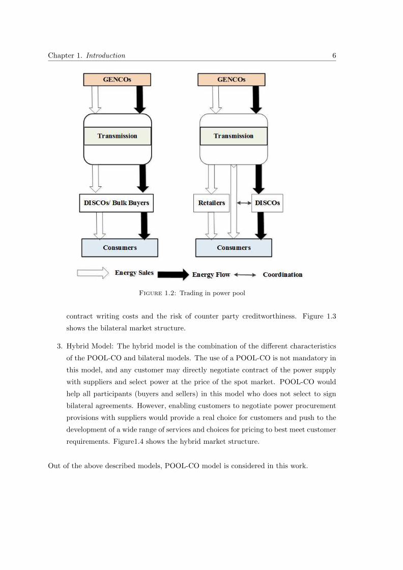
Figure 1.2: Trading in power pool
contract writing costs and the risk of counter party creditworthiness. Figure 1.3
shows the bilateral market structure.
3. Hybrid Model: The hybrid model is the combination of the different characteristics
of the POOL-CO and bilateral models. The use of a POOL-CO is not mandatory in
this model, and any customer may directly negotiate contract of the power supply
with suppliers and select power at the price of the spot market. POOL-CO would
help all participants (buyers and sellers) in this model who does not select to sign
bilateral agreements. However, enabling customers to negotiate power procurement
provisions with suppliers would provide a real choice for customers and push to the
development of a wide range of services and choices for pricing to best meet customer
requirements. Figure1.4 shows the hybrid market structure.
Out of the above described models, POOL-CO model is considered in this work.
Chapter 1. Introduction 7
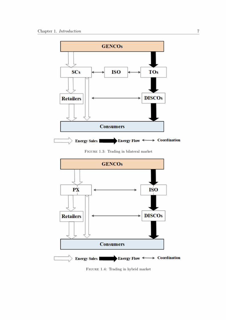
Figure 1.3: Trading in bilateral market
Figure 1.4: Trading in hybrid market

Chapter 1. Introduction 8
1.3.3 Key Components in Strategic Bidding Procedure
The electric industry’s setup has changed from a vertically integrated manner to a com-
petitive market manner globally. The generation, transmission and distribution activities
were managed and functioned in the traditional system by a single, centralized utility
operator that ensures energy flow to customers throughout the service area. Operation of
the vertically integrated power system is based on achieving possible cost-effective solution
while meet the requirements of security and reliability. But there are different problems
associated with deregulated power industry and new system operation standards. Because,
in the deregulated market, numerous entities are developed. Several system operation ac-
tivities were taken over by many entities such as GENCOs and the market operator. In
this market, everyone has to play independently while maintaining system reliability and
security. In the power market, GENCOs, customers and ISO are key players [2, 5].
The main goal of GENCOs is to maximize their own profit. Due to this reason, firstly,
the GENCO must make a precise system forecast, containing its price and its load. Sec-
ondly, the GENCO should have a good bidding strategy based on the forecasted system
information in order to achieve the maximum profit.
In a restructured system, customers are no longer obligated to purchase any services from
their local utility company. Customers would have direct access to generators or contracts
with other providers of power, and choose packages of services (e.g., the level of reliability)
with the best overall value that meets customers’ needs.
ISO plays a major role in market operations as well as in security operations in deregu-
lated electrical power systems operating with the pool type of structure [7]. Also, ISO’s
responsibilities are to operate the market in a safe and efficient manner and to monitor the
market free of market power. Therefore, first, the ISO must accurately predict the system
load to ensure that there is sufficient energy to satisfy the load and sufficient ancillary
services to ensure the physical power system’s reliability. Second, the ISO’s operational
responsibilities include the energy market, the market for ancillary services, and the mar-
ket for transmission. To fulfill these responsibilities, ISO must be equipped with powerful
tools. Third, to suppress market power and protect market participants, the ISO must be
equipped to monitor the market.

Chapter 1. Introduction 9
1.4 Literature Review Focused on Bidding Strategies in an
Emerging Electricity Market
The power system restructuring has changed the power system function significantly, re-
sulting in significant competitive, technological and regulatory modifications. In deregu-
lated markets, the function of strategic bidding plays a vital role in optimizing the profit of
the competition participating entities [8]. Moreover, Strategic bidding problems from the
point of view of power suppliers and large buyers, this type of transition is also justified by
the current situation as an inevitable social welfare necessity. Therefore, in the economic
operation of deregulated power systems, strategic bidding problems in the auction markets
play an important role. In recent times many researchers have carried out their research
over strategic bidding.
The power supplier (PS) is a price-taker in a perfect electricity market. For a supplier,
the optimal bid strategy is simply to bid marginal costs. When a power supplier bids to
exploit market imperfections to increase profits other than marginal production costs, the
behavior is called strategic bidding [9, 10]. If the power supplier can increase its profits
successfully through a strategic bid or any other way than to reduce its costs, it is said
that it has market power [9]. The emerging markets for electricity are certainly not per-
fectly competitive, resulting in a supplier being able to increase profits through strategic
bidding or, in another way, through exercising market power. The problem of optimal
bidding strategies for competitive PSs was first introduced by David [10] and the author
observed that there was some factor that may influence these bidding strategies. Some of
them are rival’s behaviour, supplier production cost, deviation in demand, and operating
constraints or some regulatory constraints. Among these, most uncertain is the bidding
behaviour of rival suppliers due to the natural behaviour of members who play to expand
their benefit. This may intensify the troubles in bidding decision process. In [11], [12],
authors have assumed that the electricity providers are free to charge their marginal pro-
duction expenses and submit single hour [11] and multi hour [12] linear bidding features,
and are paid the MCP once their offers have been selected. The bidding issues are formu-
lated as a stochastic optimization operation and solved by using Monte Carlo (MC) [11]
and Refined Genetic Algorithm (RGA) [12], respectively. Moreover, in these works rivals
bidding behaviours are presented as a discrete nature. Therefore, a comprehensive work
has been done on the development of strategic bidding while considering the generation
side participation. In [13], authors study the spot market bidding decision-making issue
and to calculate the probabilities of change and benefits for the Markov Decision Process

Chapter 1. Introduction 10
(MDP) model, an algorithm is created. A conceptual research is conducted on the procure-
ment policies of energy providers in electricity market, using the step-by-step procurement
protocol [14]. A uniform price spot market in which all winning supply bidders receive the
same price for market clearing and other competing generators’ offers (rivals) are based on
the features of probability distribution is considered in [15]. In [16], authors have suggested
to apply the Particle Swarm Optimization (PSO) technique for strategic bidding on the
oligopolistic power market by an electricity provider. For both block bidding and linear
bidding, the power market model was postulated. Optimization model for Strategic Bid-
ding Problem (SBP) is proposed in [17] and show how to fix it using a decomposition-based
PSO technique. The inertia weight approach particle swarm optimization (IWAPSO) has
been proposed to solved optimal bidding strategy for power suppliers and the anticipat-
ed maximization of profit and minimization of risk (profit variance) are mixed into the
objective function of the issue of optimization in [18]. The Ant Colony Optimization al-
gorithm was suggested to model the bidding behaviours of power market providers with
a step-by-step bid function in [19]. In [20], authors have proposed a new technique using
a combination of PSO and Simulated Annealing (SA) to predict the Generating Compa-
nies (GENCOs) bidding approach in the electricity market where they have incomplete
information about their rivals and the industry payment mechanism is paid as an offer.
A novel self-organizing hierarchical particle swarm optimization with time-varying accel-
eration coefficients (SPSO-TVAC) solves the objective function of the GENCO including
the anticipated profit maximization and risk minimization and the MC strategy is used
to simulate the conduct of competitors in [21]. From a GENCO’s point of view, Genetic
Algorithm (GA) has been proposed in [22] for bidding approach in a day-to-day market to
maximize one’s own profit as a market participant. Fuzzy Adaptive Gravitational Search
Algorithm (FAGSA) has been presented to solve the optimum bidding strategy problem
in a pool-based electricity market in [23]. The optimal bidding strategy problem has been
solved by using shuffled frog leaping algorithm (SFLA) in [24, 25]. in [26], authors have
presented various metaheuristic algorithms such as GA, SA and HSAGA to simulate w-
holesale electricity bidding strategies using the Nash equilibrium idea and compare the
algorithm efficiency. A Global Self-Adaptive Harmony Search Algorithm (SGHSA) is used
to achieve optimum bidding approaches in [27]. Differential Evolution (DE) algorithm is
proposed to solve the problem of bidding strategy in the operation of power systems in
a deregulated environment in [28]. Invasive Weed Optimization Algorithm (IWOA) has
been implemented to tackle the issue of the optimal bidding strategy in [29]. It is worth
mentioning that in the above discussed literature, heuristic and metaheuristic approaches
have been adopted to solve the different strategic bidding problems. Also, rivals’ bidding

Chapter 1. Introduction 11
behaviors are represented as a discrete probability distribution function. Moreover, sup-
plier profit maximization objective function represented as non-linear due to unknown or
stochastic bidding parameters. Therefore, depending on the bidding models, objective
function and constraints may not be differentiable; in that case conventional methods
cannot be applied, whereas, heuristic and metaheuristic methods could be applied [23].
Heuristic and metaheuristic methods are basically based on the tuning of its parameters
and thus the techniques having less tuning parameter results in the most accurate results.
The trend of hybridizing and metaheuristic algorithms has been increased over the years.
Beside this linear, block and step wise bidding function with the generation limit con-
straints have also been considered in strategic bidding problem. This consideration is not
pragmatic as real-time generation is limited by ramp rates; this would affect the operation
of generating units [30], [31], which is critical to ensure practical optimal results. Thus,
to obtain the practical optimal solution, the generators with ramp rates consideration are
essential.
In the literature, most of the researchers have focused on supplier’s side strategic bid-
ding problem; limited work has been carried out on the demand side. Based on this, [32]
proposed a strategic bidding problem together for power suppliers and large consumers.
Thereafter, [33–38] attempted and solved the problem of PS and large buyer profit maxi-
mization by determining both entities bidding parameters. In an emerging power market,
when both entities; suppliers and buyers; participate in double sided bidding for profit
maximization, problem becomes a multi-objective strategic bidding problem in which two
objectives are simultaneously optimized. This is because of the nature of the power sup-
pliers and buyers. The power suppliers try to increase the MCP by withholding capacity
from the market and the large buyers try to decrease the MCP by adjusting their power
consumption. As these objectives are contradictory, a specific multi-objective problem
design is essential. By assigning weights [39–42] or multiplying them with a penalty func-
tion [43], many multi-objective formulations considering multiple goals are converted into
a single-objective problem. The normally utilized structures for multi-objective formula-
tion may incorporate weighted sum [39–42], goal programming [44], penalty function [43],
epsilon-constrained [45] based methodologies. However, these techniques have a few re-
strictions, for example, the ideal arrangement of the weighted sum methodology relies
upon the choose weights, pre-specified goals must be allotted in goal programming, and a
master and slave goals are required to be determined in epsilon constrained approaches.
The above discussed methods suffer from some more limitations which can be overcome
by scaling the objectives through the different approaches like fuzzification [46], max–min
approach [47], and fuzzy-based goal programming [48], but they may be lacking the inbuilt

Chapter 1. Introduction 12
mechanism to deliver the desired Pareto-front. Therefore, more powerful multi-objective
solution approaches are required.
During the recent years, the renewable energy usage around the globe has been on the
upward swing due to low carbon emission. Electrical power productions and percent of
installed capacities of wind and solar power plants go higher and will turn into the signifi-
cant power generators soon. Owing to this reason, Renewable Energy Sources (RESs) are
under prime concern with the annihilation of fossil fuels along with carbon emissions. This
has led to new dimensions of exploration in optimal bidding strategy with amalgamation of
wind and solar based power generation, which further draw the interest of researchers. As
a part of the strategic bidding of conventional generators, the GENCOs having renewable
generation also participates in the bidding process. It provides market fairness and better
utilization of RESs in the deregulated market [49]. Wind and solar power generation have
been the first choices due to its low cost, among all types of RESs. The main disadvan-
tages of wind and solar power production are its uncertainty and unpredictable nature of
wind speed and solar irradiations which always result in deviation from the actual gen-
eration. In the deregulated environment, the uncertainties of wind and solar power have
increased the problems manifold for the producers in devising an optimal bidding strategy
with CPS. A comprehensive work has been done on the development of strategic bidding
while considering the wind PSs participation. A bidding strategy considering wind PSs
with conventional generators in a deregulated electricity market is proposed [50–52]. The
effect of wind generation on electricity prices has been investigated by [53]. However, the
variability has not been evaluated by considering any uncertainty model in [50–53]. More-
over, [54] has considered a probabilistic strategy for evaluating the electricity cost in the
market for wind generators associated with wind prediction errors. On the basis of the
concept presented in [54], the penalties associated with the deviation between forecasting
and actual production of wind power is considered in [55–57]. Uncertain wind power out-
put increases the imbalance cost and penalties associated with wind farms. This result
reduces the revenue for wind PSs. Other renewable power sources such as Solar Photo-
voltaics (SPVs) have also been considered in bidding strategy [58–62]. However, these
works have not considered uncertainty associated with SPV. The main disadvantages of
wind and solar power production are its uncertainty and unpredictable nature of wind
speed and solar irradiations which always results in deviation from the actual generation.
In the deregulated environment, the uncertainties of wind and solar power have increased
the problems manifold for the producers in devising an optimal bidding strategy with
CPS. Uncertain wind and solar power output increases the imbalance cost and penalties
associated with wind and solar farms. This result reduces the revenue for wind and solar
Chapter 1. Introduction 13
PSs. Therefore, the actual modeling of the uncertain wind power is essential to minimize
the imbalance and increase the profit.
The deregulated electricity markets raise the importance of coordination of bidding strate-
gies in the energy and reserve services market. The effect of coordinated bidding strategies
in the energy and reserve services market has been investigated by many researchers. In
these two markets, the single sided bidding is utilized in which an energy prices inclusive
of other cost either fixed or variable is offered, and a simple market clearing process based
on the intersection of supply and demand bid curves is used to determine the winning bids
and schedules for each hour. The problem of developing optimally coordinated bidding
strategies in day-ahead energy and spinning reserves for competitive power suppliers has
been presented in [63]. Furthermore, assumed that energy market and reserve market
is cleared independently and simultaneously for 24 supply hours [64] and single supply
hours [65]. Thereafter, [66–71] attempt these problems for profit maximization of the
power suppliers in energy and reserve market and an extensive review of different model-
ing and dispatching method for focusing energy and reserve markets is presented [72] and
concluded that the inclusion of additional variables and constraints significantly increases
the size of the problem and hence the expected calculation times. These disadvantages
will certainly be some of the challenges facing future work.
1.5 Research Objectives
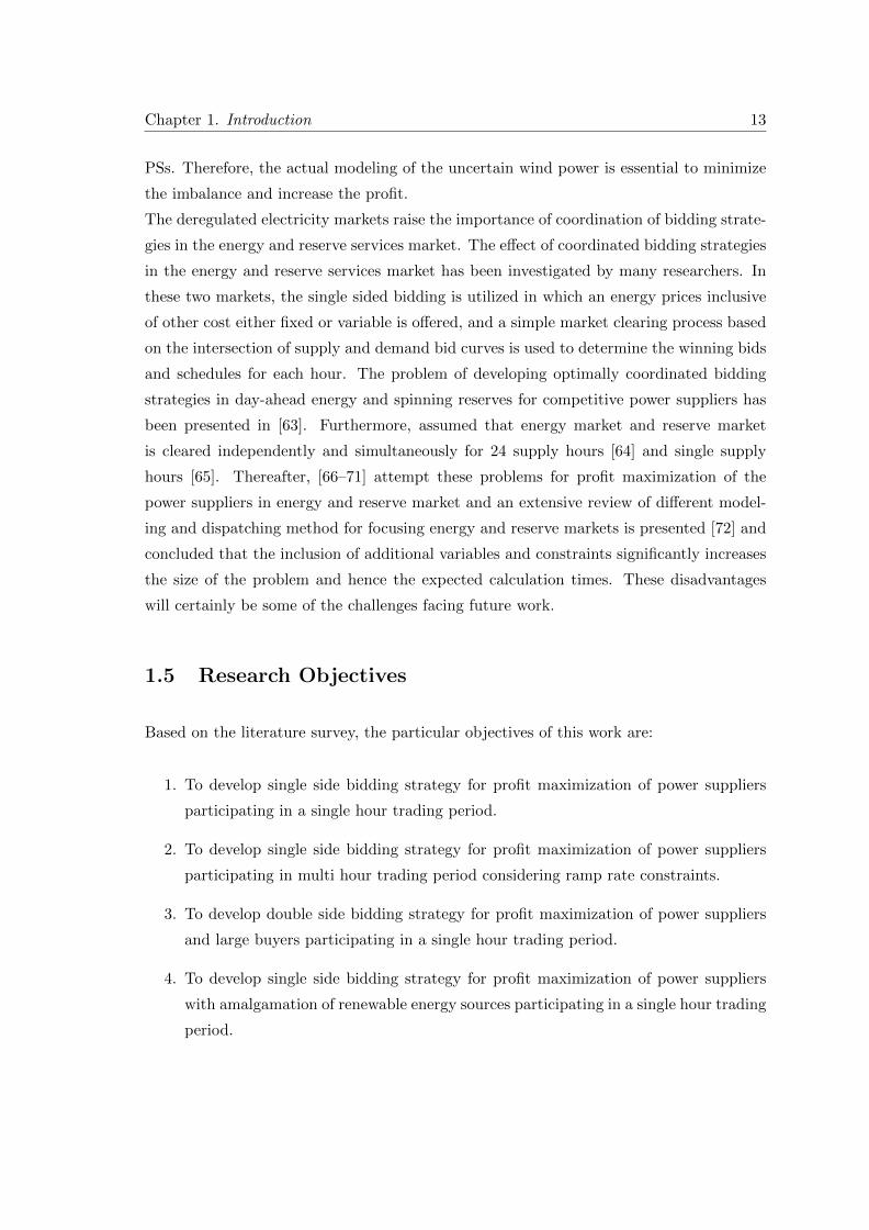
Based on the literature survey, the particular objectives of this work are:
1. To develop single side bidding strategy for profit maximization of power suppliers
participating in a single hour trading period.
2. To develop single side bidding strategy for profit maximization of power suppliers
participating in multi hour trading period considering ramp rate constraints.
3. To develop double side bidding strategy for profit maximization of power suppliers
and large buyers participating in a single hour trading period.
4. To develop single side bidding strategy for profit maximization of power suppliers
with amalgamation of renewable energy sources participating in a single hour trading
period.

Chapter 1. Introduction 14
5. To develop double side bidding strategy for profit maximization of power suppliers
and large buyers with amalgamation of renewable energy sources participating in a
single hour trading period.
6. To develop coordinated bidding strategy between energy and reserve markets in a
single hour trading period.
1.6 Thesis Contributions
This study takes the restructured electricity market operation considering the strategic
bidding problem only. Strategic bidding in restructured electricity markets are further
confined into strategic bidding in single sided POOL-CO model, double sided POOL-CO
model with and without amalgamation of renewable energy sources and coordinating bid-
ding strategy between energy and reserve markets.
Strategic bidding models appropriate for single and double sided POOL-CO markets are
considered. The strategic bidding in both single and double sided POOL-CO markets
are done by ISO based on uniform MCP. Moreover, an Oppositional Gravitational Search
Algorithm (OGSA) has been implemented in order to optimize the single hour trading
period bids in single-sided POOL-CO market to maximize the individual GENCO profit.
Meanwhile, the ramp rate limits are considered for multi-hour trading period and opti-
mized bids are obtained using OGSA. Moreover, in order to deal with GENCO’s profit
maximization issue, the information of opponent bid is solved utilizing joint normal prob-
ability distribution function. Notably, the profit of each power supplier can be maximized
if the optimized bids are submitted to ISO and the participation of generators in a day
ahead electricity market bidding process without considering ramp rate limits will cause
economic loss to the generators as this extra cost is beared by generators. Further, double-
sided bidding strategy is formulated as multi objective with the objective of social welfare
maximization. A Technique for Order of Preference by Similarity to Ideal Solution (TOP-
SIS) along with OGSA has been implemented in order to optimize the single hour trading
period bids in double-sided POOL-CO market to maximize the profits of the individual’s
power supplier and large buyer. A standard IEEE 30-bus with two large consumers is
considered in single hour trading period. Moreover, in order to deal with large consumers
profit maximization issue, the information of opponent bid is solved utilizing joint normal
probability distribution function. It is found that, proposed TOGSA increases the trading
of power between suppliers and buyers, and also maximize the social welfare.
The single and double sided bidding strategies with amalgamation of renewable (such as

Chapter 1. Introduction 15
wind and solar) energy sources participating in single hour trading period are proposed.
Wind and solar are used as probabilistic manner to model the uncertainty and their pre-
diction error are considered in cost function using underestimation and overestimation.
Furthermore, the uncertainty of the behaviour of rival is minimized using the function of
normal distribution of probability. The uniform MCPs in both types of bidding model
with the presence of renewable energy sources are calculated. The proposed bidding s-
trategies are analytically tested on standard IEEE 30 and 57 bus systems respectively. It
is found that, incorporating wind and solar power also affects the bid as it reduces the
CPS generation and provides less MCP value that would deliver sufficient electricity from
accepted sales bids to meet all accepted purchase bids and increase the total traded power.
Further, it is also found that, the overestimation of uncertainty is very less as compared
to the underestimation in both the solar and wind power generation. This will encourage
the solar and wind power suppliers for bidding the extra power into the real-time market
if the underestimation is positive.
A suitable bidding strategy is indispensable for power suppliers in the energy and reserve
services market is considered. The uniform MCPs in both markets are calculated. Further-
more, the uncertainties of the behaviour of rival in both markets are minimized using the
function of normal distribution of probability. The coordinated bidding strategy for profit
maximization of competitive power suppliers in an energy and reserve market has been
solved using OGSA. The proposed algorithm was tested on 6 supplier system considering
1 supplier as main generator and other 5 as its rival generators. The results indicate the
increase in profit of the main generator and it’s MCP in both markets.
1.7 Outline of The Thesis
This thesis is divided into 6 Chapters. Chapter 1 discusses the hierarchy, structure, and
functioning of electricity markets and provides an insight into the state-of-the-art opti-
mal bidding strategies in an emerging electricity market. A detailed literature survey
focused on the existing bidding strategies such as single side for profit maximization of
power suppliers, double side for profit maximization of power suppliers and large buyers,
bidding strategies for renewable power suppliers, and coordination of bidding strategies
in day-ahead energy and reserve markets for profit maximization of power suppliers has
been presented. Moreover, the detailed literature survey also focused on existing solution
methods of bidding strategies, along with the limitations of these existing methods, has
been presented. On the basis of literature survey, the research objectives have been for-
mulated. Additionally, the major contributions of the thesis work have been included in

Chapter 1. Introduction 16
this Chapter.
In Chapter 2, optimization techniques such as Oppositional Gravitational Search Algo-
rithm (OGSA) and Technique for Order of Preference by Similarity to Ideal Solution
(TOPSIS) along with OGSA (TOGSA) to solve different strategic bidding problems has
been discussed.
In Chapter 3, presented single side bidding strategy for profit maximization of power sup-
pliers participating in a single hour and multi-hour trading period and double side bidding
strategy for profit maximization of power suppliers and large buyers participating in a
single hour trading period.
In Chapter 4, optimum bidding strategies such as single-side for power supplier and dou-
ble side for power suppliers and large buyers have been formulated with amalgamation of
substantial wind and solar based power generation. Moreover, the wind and solar are used
as probabilistic manner to model the uncertainty and their prediction error are considered
in cost function using underestimation and overestimation.
In Chapter 5, optimal coordinated bidding strategy between energy and reserve markets
is considered for six generating units system considering 1 supplier as main generator and
other 5 as its rival generators. The considered framework is utilized to obtain the maxi-
mum profit for power suppliers.
In Chapter 6, conclusions and future scope of the proposed research work are discussed.

Chapter 2
Optimization Techniques to Solve
Strategic Bidding Problems
2.1 Introduction
Problems involving global optimization throughout the scientific community are omnipresen-
t. In fields such as engineering, statistics and finance, global optimization is needed. But
numerous practical problems have non-linear, non-continuous, non-differentiable, noisy,
multi-dimensional, flat, constraints or stochastic functions. Such problems are challenging
and cannot be analytically solved. The standard method to an optimization issue starts
with the design of an objective function that can shape the goals of the problem while
incorporating any limitations. The standard methods of optimization are linear program-
ming, dynamic programming, gradient search and other related methods. These standard
methods have difficulty dealing with the complexities of problems in the real world. Users
usually require three requirements to be met by a practical optimization technique. First-
ly, the method should find the global solution irrespective of the parameter values of the
initial system. Secondly, there should be rapid convergence. Third, a minimum number of
control parameters should be available to the program to make it easy to handle. Oppo-
sitional Gravitational Search Algorithm (OGSA) and a Technique for Order of Preference
by Similarity to Ideal Solution (TOPSIS) along with OGSA can fulfill all above mentioned
requirements. Therefore, they are used to solve problems in the real world.
17

Chapter 2. Optimization Techniques to Solve Strategic Bidding Problems 18
2.2 Oppositional Gravitational Search Algorithm (OGSA)
Gravitational Search Algorithm (GSA) [73] implementation for power system problems
provides high-quality results [74–78] as this algorithm have the best tunable parameters.
Its most extensive feature is an adjustment of gravitational constant for improvement of
the search accuracy. It provides a fast solution with high-quality results [79]. In GSA tech-
nique, the initialization of population is configured randomly, and the activity approach
of different parameters is dependent on randomness. If the random guess is not far away
from the optimal result, convergence can be achieved quickly. However, on the contrary
the random guess may be far away from the optimal result. This pessimistic scenario will
lead to an additional wastage of time while searching for optimal solution or in worst case
may end up resulting in non-optimal solution. In fact it is impossible to make a best initial
guess without having any previous knowledge about the situation. Therefore, logically we
should be looking for all possible options or more precisely we must look in the oppo-
site direction also. Considering this fact, in GSA, oppositional population based learning
(OBL) concept [80] is incorporated. The utilization of opposite agents in the evaluation
process of GSA enables enhanced exploration of the search space. This prevents trapping
of the search in local optimal solution. A step-by-step procedure of OGSA to solve the
problem of optimization is as follows:
1. Initialization of Population: Assume a system consist of N agents (masses), position
of the yth agent is represented by:
λy = (λ1y, ......, λ
Dy , ......., λ
My ) (2.1)
where, λDy ∈ [LDy , UDy ] is the yth agent position in the Dth dimension and M is the
dimension of search space and LDy , UDy are lower bound and upper bound limits of
yth agents in the Dth dimension.
2. Opposition phenomenon in GSA: In [80], authors have presented opposition based
learning phenomenon. In that work, the authors have considered the current and
opposite agents in order to get a better estimation of current agent result. It is
concluded that an opposite agent provides better optimal solutions compared to
that of random agent solutions. The opposite agents positions (Oλy) are completely
defined by components of λy
Oλy = [Oλ1y, ......, Oλ
Dy , ....., Oλ
My ] (2.2)
Chapter 2. Optimization Techniques to Solve Strategic Bidding Problems 19
where, OλDy = LDy + UDy − λDy with OλDy ∈ [LDy , UDy ] is the position of yth opposite
agent Oλy in the Dth dimension of oppositional population.
3. At the OGSA starting an iterative process, a joint population of {λ,Oλ} is generated
with all the constraint is satisfied. Selection strategies are used to select the N
number of fittest agents from the joint population set of {λ,Oλ} generated current
population λ as follow:
λy(i) =
Oλy(i) if fit(Oλy(i) > fit(λy(i))
λy(i) otherwise(2.3)
The algorithm simultaneously evaluates the fitness of an agent and its opposite
agent. The agent with better fitness value is used in further computation and the
other agent is discarded.
4. Acceleration of agents: The fitness evaluation is used to calculate the mass of each
agent in GSA. The mass of each agent is calculated as follows:
My(i) =my(i)N∑l=1
ml(i)
(2.4)
here, my(i) =fity(i)−worst(i)best(i)−worst(i)
where My(i) is the normalized mass of yth agent at ith iteration and worst(i), best(i)
are the worst and best fitness of all agents at ith iteration.
The acceleration aDy (i) acting on yth agent at ith iteration is evaluated follows:
aDy (i) =∑
l∈Gbest,l 6=y
randl G(i)My(i)
Ryl(i)+E(λDl (i)− λDl (i)) (2.5)
where set of first 2% agents are Gbest with best value of fitness and greatest mass
randl is the uniform random number between interval (0, 1). Ryl(i) is the Euclidean
distance between two agents yth and lth at ith iteration and E is a small positive
constant. The gravitational function G(i) is represented by
G(i) = G×
1− iteration
Total iteration
(2.6)
here, G = c maxD∈{1,2,.....,M}
(|λDU − λDL |
)where c is search interval parameter

Chapter 2. Optimization Techniques to Solve Strategic Bidding Problems 20
5. Update the position and agents velocity: In next (i+ 1)th iteration, the position and
agents velocity is calculated as follows{vDy (i+ 1) = randy × vDy (i) + aDy (i)
λDy (i+ 1) = λDy (i) + vDy (i+ 1)(2.7)
where randy is a random number between interval (0, 1), vDy (i) is the velocity of yth a-
gent at Dth dimension during ith iteration and λDy (i) is the position of yth agent at Dth
dimension during ith iteration.
2.3 Technique for Order of Preference by Similarity to Ideal
Solution (TOPSIS)
Recently, TOPSIS has been introduced in [81–85] for providing uniformly distributed
Pareto front of multi-objective problems. The approach applies Euclidean geometry to
offer uniform distribution of result for multi-objective optimization problems as compared
to available methods. In this method, Euclidean distances of individual solutions are
minimized from its excellent set of solutions; known as Positive Ideal Solution (PIS), while
simultaneously maximizing the distances from worst set of solutions, known as Negative
Ideal Solution (NIS). This method can be combined with any recent heuristic optimization
method to choose the best compromising result at some point of iterations of technique.
2.3.1 Multi-objective Problem Formulation using TOPSIS Technique
All objectives of the problem can be represented as
Maximize
[O1(x),O2(x), ..............., On2(x)] (2.8)
Subject to x ∈ S
where, Oi(x) : Rn → R is ith objective, i = 1, 2, ......., n2, n2 > 1, and S is space of the
search.
As mentioned, TOPSIS technique is implemented to frame and solve the multi-objective
double sided strategic bidding problem for profit maximization of the suppliers and large
buyers. In this technique, Euclidean geometry is applied, and two reference points like PIS

Chapter 2. Optimization Techniques to Solve Strategic Bidding Problems 21
and NIS are used to find best compromising result. Therefore, choice of the alternative
result should be at nearest Euclidean distance from PIS and farthest from NIS. Using
this procedure, the solutions remain concentrated around their individual best solution.
This enables higher quality of results for actual multi-objective optimization problems. In
TOPSIS technique following steps are used to solve multi-objective problems:
1. Frame a standardized selection matrix to transform all dimensional functions in to
non-dimensional functions. The factors of matrix may be represented by
Fab =Oab√n1∑a=1
O2ab
∀ a ∈ n1 & b ∈ n2 (2.9)
where, n1 is the number of elements and Oab is the value of ath element of bth
objective.
2. A weighted standardized selection matrix may be built to offer weights to the objects
if required. The step can avoid if all objects are similarly significant. The factors of
the matrix are represented by
Wab = wb × Fab ∀ a ∈ n1 & b ∈ n2 (2.10)
where, wb is weight of the bth objective andn2∑b=1
wb = 1.
3. To maintain the best and worst solutions of the each objective, PIS and NIS are
calculated and expressed as:
PIS ={W+
1 ,W+2 ,W
+3 , ............,W
+n2
}(2.11)
NIS ={W−1 ,W
−2 ,W
−3 , ............,W
−n2
}(2.12)
where, W+b =
{max 〈Wab〉 ∀ a; if object denotes a profit
min 〈Wab〉 ∀ a; if object denotes a benefit
W−b =
{max 〈Wab〉 ∀ a; if object denotes a benefit
min 〈Wab〉 ∀ a; if object denotes a profit
4. For every opportunity from PIS and NIS, Euclidean distances db+ and db− are
measured and given by:
d+b =
√√√√ n2∑b=1
(Wab −W+
b
)2& d−b =
√√√√ n2∑b=1
(Wab −W−b
)2(2.13)
Chapter 2. Optimization Techniques to Solve Strategic Bidding Problems 22
5. The Relative Closeness Index (RCI) can be measured for individual opportunity
using the value from Step 4.
RCI+a =
d+a
d+a + d−a
(2.14)
The best compromising results may be selected from RCI. Whose alternatives have
highest RCI value will be selected as the best compromising result.
2.4 Conclusion
Several techniques of heuristic optimization have been introduced in recent years. Some
of these techniques are inherently inspired by swarm behaviors. A modified optimization
technique is introduced in this Chapter, which is called OGSA. OGSA is based on oppo-
sition learning phenomenon. This technique considers both the current and the opposite
agent position in order to obtain better estimate of agent position. The opposition oper-
ator in OGSA helps to provide search space, where the GSA fails to reach. It helps to
avoid the search to get trapped at local optimal solution.
To obtain the most compromising solution for contradictory multi-objectives optimization
problem, recently, TOPSIS along with OGSA (TOGSA) has been also introduced in this
Chapter. This method extends Euclidean geometry to give for multi-objective optimization
problems a uniform distribution of results. This technique minimizes Euclidean distances
from its outstanding set of alternatives ; known as PIS, while maximizing distances from
the worst set of alternatives, known as NIS.
In the next Chapter, the optimal bidding strategies in single side and double side trading
mechanisms have been investigated using proposed OGSA and TOGSA respectively for
maximization of the profit for market participants. In addition, the performances of the
proposed techniques have been compared with the existing results based on available
different methods in the literature.

Chapter 3
Bidding Strategies for Electricity
Market Participants
3.1 Introduction
The bidding strategies employed by different market participants in an emerging power
market environment have substantial influences on their profits/benefits and a power mar-
ket’s operating behavior. The power market is continuously growing after deregulation in
electricity market structures since 1980 and introduces competition among all entities in
energy market. Moreover, unbundling of vertically integrated electricity market creates
open access environment for network access which encourages the development of new
technologies to build a competitive electricity market to improve its performance [5]. But
the unexpected changes in electricity market introduce imperfection in the market. In
microeconomics theory, market participants take advantage of imperfections to increase
profits through bidding in the market. Theoretically, they maximize their benefits through
bidding a price equal to their expenses of their marginal seller and buyer cost. But prac-
tically, they have higher bidding prices over their marginal selling and buying cost [2].
Power market structure is essential to accommodate market entities in the system for
making power transactions. Various models have been developed based on trading strate-
gy and number of participants to ensure secure and economical operation. Among all the
classical models discussed in the scientific literature, power POOL-CO model is extensive-
ly utilized for centralized trading between buyers and sellers. In this model, sellers and
buyers of electricity typically submit the sealed bids to the pool for the amounts of power
they are willing to trade in the electricity market. However, due to the limitation of sealed
23

Chapter 3. Bidding Strategies for Electricity Market Participants 24
bids, the sellers and buyers are found to be facing problems such as uncertain behavior
of rivals. These problems are known as a strategic bidding problem [9, 10]. In this sense,
sellers and buyers can exercise strategic bidding to achieve the maximum profit. Therefore
in this chapter, optimum bidding strategies such as single sided for power supplier and
double sided for power suppliers and large buyers have been formulated to achieve the
maximum profit of power supplier and large buyer.
3.2 Market Clearing Mechanism in a POOL Based Energy
Market
The market participants submit their bids to the central POOL-CO mechanism market
structure. There are two type of central POOL-CO bidding mechanisms namely; single-
sided market structure and double-sided market structure, which are taken into account
in this chapter. Single-sided bidding POOL-CO mechanism allows only power suppliers
to participate in the energy markets. They can submit their energy supply bids to the
PX-managed energy market whereas, the system operator manages the transmission facil-
ities. The ISO controls the system operator, PX, and receives bids of energy from power
suppliers. After that the generation outputs sets are calculated to meet the requirement
of demand. In the double side bidding mechanism, both suppliers and large buyers are
permitted to submit their bids to the central pool [6]. In this mechanism ISO receives
electricity transaction bids from power suppliers as well as large buyers and economically
dispatch them based on their price and MW bids. These operations are carried out in in-
direct ways which is governed by the pool operator. Both power suppliers and large buyers
send their bids to the ISO, and then ISO determines the bids based on the MCP as a sole
decision maker. There are various ways to define MCP in the central POOL type market.
In this context, the most common method is the uniform price method where the point
of market equilibrium occurs at the intersection of the supply and demand incremental
cost curve [86]. It is noteworthy that both power suppliers and large buyers optimize their
bidding data with the objective of their peculiar profit maximization before submitting
bids to the pool operator and then provide the optimized proposals to the ISO. Further,
it can also estimate the bidding value of the rival by using the joint normal Probability
Distribution Function (PDF) [11].
Chapter 3. Bidding Strategies for Electricity Market Participants 25
3.2.1 Single-sided POOL Based Energy Market
In a single-sided POOL based energy market, each PS is required to submit a bid as a
non-decreasing linear supply function to the POOL [11]. The linear non-decreasing supply
bid function of the mth power supplier can be represented as
αm,t + βm,tPGs,m,t = Rs,t (3.1)
The linear non-decreasing supply bid function given in equation (3.1) includes different
constraints such as
1. Power balance constraints: The constraint of the power balance is a constraint of
equality that reduces the power system to a fundamental principle of equilibrium
between the total generation of GENCO participating in the electricity markets and
the customers’ demand profile.
PS,T∑m=1,t=1
PGs,m,t = D (Rs,t) (3.2)
2. Forecasted demand constraints: It is said that the demand for electricity is elastic if a
change in price percentage demand results in a larger change in demand percentage.
On the other hand, the demand is said to be inelastic if the relative change in demand
is lower than the relative price change. The forecasted demand can be calculated as
D (Rs,t) = Dc,t −K ×Rs,t (3.3)
3. Maximum and minimum power generation limits of the power generators: The power
generation units have maximum and minimum limits of production directly associ-
ated with the design of the generator, which can be defined as a pair of constraints
on inequality.
PGmin,s,m,t ≤ PGs,m,t ≤ PGmax,s,m,t (3.4)
4. Up and down Ramp rate limits of the power generators: The rate of up and down
of the generators power output is kept within scale so as to maintain thermal gra-
dients within secure limits and to obstruct decline in lifespan of the turbine. These
constraints of ramp rate can be expressed as
−RDm ≤ (PGs,m,t − PGs,m,t−1) ≤ RUm (3.5)

Chapter 3. Bidding Strategies for Electricity Market Participants 26
After receiving the supplier’s bid, pool decided the output of active power generation and
meets with the total system demand and then minimizes total buying cost. It noted that
equations (3.1)-(3.4) should satisfy the power dispatch when considering power balance
constraint (3.2) and power inequality constraints (3.4). Generally, the MCP is decided
in such a way that the supply bids and demand bids are aggregated respectively into a
supply curve and demand curve. The supply curve and demand curve intersection point
is the MCP. For the MCP calculation (3.1)-(3.3) has been taken into consideration while
(3.4) and (3.5) are neglected and can be expressed as
Rs,t =
Dc,t +PS,T∑
m=1,t=1
αm,tβm,t
K +PS,T∑
m=1,t=1
1βm,t
(3.6)
Each power supplier can calculate the power dispatch as
PGs,m,t =Rs,t − αm,t
βm,t(3.7)
For each supplier minimum and maximum generation limits are taken into account while
dispatching power. In order to participate in the market competition each supplier must
be able to provide preset minimum power requirement. However, if the supplier violates
the maximum generation limit then equation (3.4) will decide its upper limit.
3.2.2 Double-sided POOL Based Energy Market
In a double-sided POOL based energy market, each PS and large buyer is required to
submit a bid as a linear non-decreasing supply and non-increasing demand bid functions
to the POOL [32]. The linear non-decreasing supply bid function of the mth power supplier
and the linear non-increasing demand bid function of the nth large buyer can be represented
respectively as
αm,t + βm,tPGd,m,t = Rd,t (3.8)
φn,t − ϕn,tCDn,t = Rd,t (3.9)
The linear non-decreasing supply and non-increasing demand bid function given in equa-
tions (3.8) and (3.9) respectively, which includes different constraints such as

Chapter 3. Bidding Strategies for Electricity Market Participants 27
1. Power balance constraints: The constraint of the power balance is a constraint of
equality that reduces the power system to a fundamental principle of equilibrium
between the total generation of GENCO and total demand profile of customers
participating in the electricity markets.
PS,T∑m=1,t=1
PGd,m,t = D (Rd,t) +
LB,T∑n=1,t=1
CDn,t (3.10)
2. Forecasted demand constraints: The forecasted demand is claculated in similar way
of equation (3.3) and can be represented as
D (Rd,t) = Dc,t −K ×Rd,t (3.11)
3. Power suppliers and large buyers bid limits constraints: The power suppliers bid
limits can be incorporated in the same way as equation (3.4) while large buyers bid
limits can be set as follows:
PGmin,d,m,t ≤ PGd,m,t ≤ PGmax,d,m,t (3.12)
CDmin,n,t ≤ CDn,t ≤ CDmax,n,t (3.13)
After receiving the supplier’s and large buyer’s bid, pool decided the output of active power
generation and meets with the total system demand to minimize total buying cost and
maximizing social welfare. As explained in Section (2), similar procedure has been used
for MCP calculation. In this section, (3.8), (3.9), (3.10) and (3.11) has been employed to
calculate MCP whereas (3.12) and (3.13) are avoided. Mathematically it can be expressed
as
Rd,t =
Dc,t +PS,T∑
m=1,t=1
αm,tβm,t
+LB,T∑
n=1,t=1
φm,tϕm,t
K +PS,T∑
m=1,t=1
1βm,t
+LB,T∑
n=1,t=1
1ϕn,t
(3.14)
Each power supplier can calculate the power dispatch and each large buyer can calculate
the demand respectively as
PGd,m,t =Rd,t − αm,t
βm,t(3.15)
CDn,t =φn,t −Rd,t
ϕn,t(3.16)

Chapter 3. Bidding Strategies for Electricity Market Participants 28
For each power supplier and large buyer minimum and maximum generation and demand
limits are taken into account while dispatching power. If the power supplier and large buyer
violates the generation and demand limit, then equation (3.12) and (3.13) will decide its
limit respectively.
3.3 Problem Formulation in Single Side POOL Based Ener-
gy Market
In a single side POOL based energy market, only power suppliers participate in bidding
process. The aim of profit maximization of the power suppliers participating in single side
POOL based energy market and competing with other suppliers can be set as
Maximize
Profit = Revenue− Production Cost (3.17)
Revenue: Total energy sales are referred to as revenue of power supplier. It is calculated
by multiplying MCP with power dispatch. It can be represented as
Revenue = Rs,t × PGs,m,t (3.18)
Production Cost: The production cost function of the power supplier is approximated as
a quadratic function which can be represented as
PCs,m,t(PGs,m,t) = am,tPGs,m,t + bm,tPG2s,m,t (3.19)
Substitute equations (3.18) and (3.19) in to the equation (3.17). Now the modified equation
can be presented as
Maximize
Fs(αm,t, βm,t) = Rs,t × PGs,m,t − PCs,m,t(PGs,m,t) (3.20)
Subject to: Power balance constraints as given in equation (3.2) and power inequality
constraints as given in equations (3.4) and (3.5)
Chapter 3. Bidding Strategies for Electricity Market Participants 29
3.4 Problem Formulation in Double Side POOL Based En-
ergy Market
In a double side POOL based energy market, both power suppliers and large buyers will
participated in bidding process. The aims of profit and benefit maximization of the power
suppliers and large buyers are participating in energy markets and competing with other
suppliers and buyers. Similar procedure as explained in Section 3 is utilized for calculation
of power supplier profit and can be represented as
Maximize
Fd(αm,t, βm,t) = Rd,t × PGd,m,t − PCd,m,t(PGd,m,t) (3.21)
Large buyer benefit function is given as
Maximize
Benefit = Purchasing Cost− Buyer Revenue (3.22)
Purchasing Cost: The large buyers purchasing cost function can be represents as
PCd,n,t(CDn,t) = en,tCDn,t − fn,tCD2n,t (3.23)
Buyer Revenue: Large buyer revenue can be expressed as
Buyer Revenue = Rd,t × CDn,t (3.24)
Substitute equations (3.23) and (3.24) in to the equation (3.22). Now modified equation
can be represented as
Fd(φn,t, ϕn,t) = PCd,n,t(CDn,t)−Rd,t × CDn,t (3.25)
Subject to equations (3.10) , (3.12) and (3.13)
In the literature, rivals bidding behaviors are represented as a discrete probability distribu-
tion function to the solution of strategic bidding model. The objective functions depicted
in (3.20), (3.21) and (3.25) subject to the given constraints. These objective functions are
behaving as non-linear functions with unknown stochastic constraints. To solve this non
linear problem heuristic approach is considered over classical methods.
Bidding data of participants in both type of sealed bidding model for next duration is
confidential. Therefore, participants do not have information about other participant’s
bid. However, last duration bidding data information is available, based on this data, es-
timation of MCP is possible. Each participant tries to estimate other participants bidding
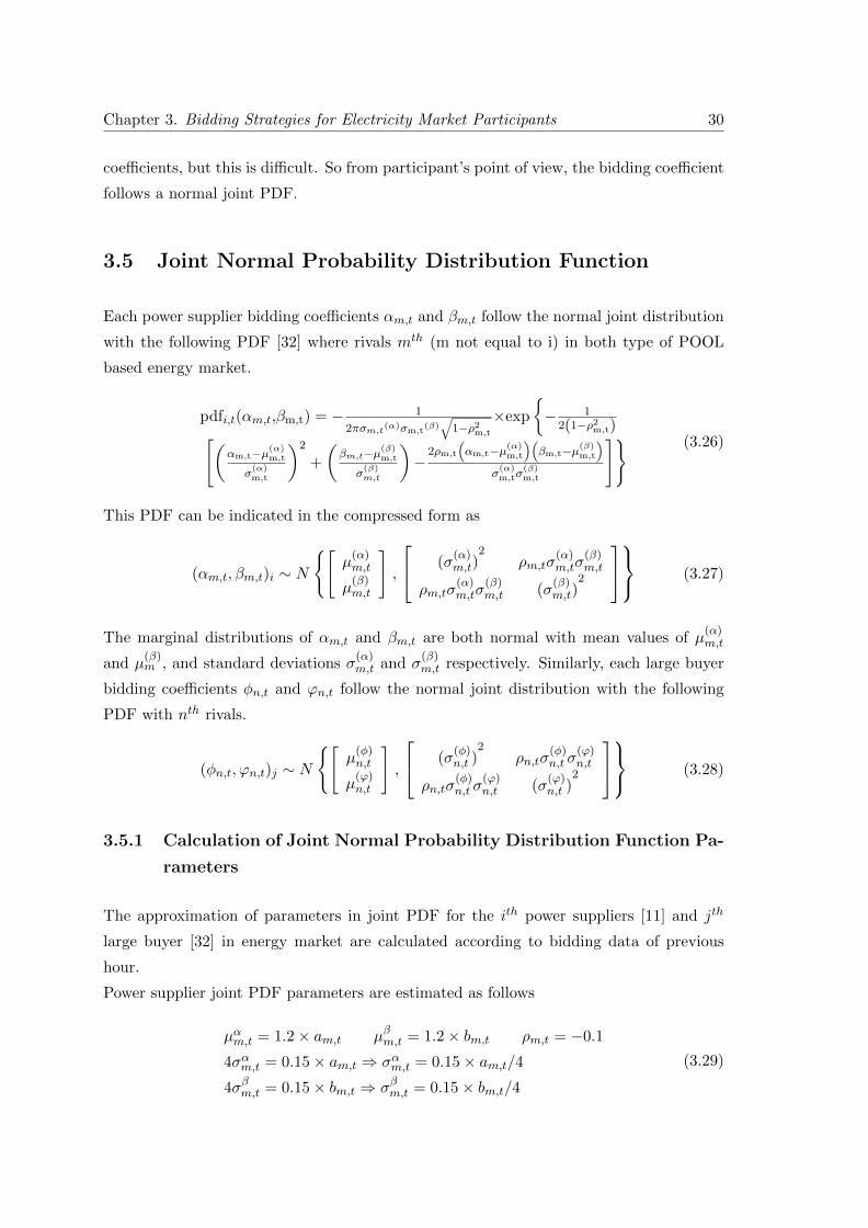
Chapter 3. Bidding Strategies for Electricity Market Participants 30
coefficients, but this is difficult. So from participant’s point of view, the bidding coefficient
follows a normal joint PDF.
3.5 Joint Normal Probability Distribution Function
Each power supplier bidding coefficients αm,t and βm,t follow the normal joint distribution
with the following PDF [32] where rivals mth (m not equal to i) in both type of POOL
based energy market.
pdfi,t(αm,t,βm,t) = − 1
2πσm,t(α)σm,t(β)√
1−ρ2m,t
×exp
{− 1
2(1−ρ2m,t)[(
αm,t−µ(α)m,t
σ(α)m,t
)2
+
(βm,t−µ(β)
m,t
σ(β)m,t
)−
2ρm,t
(αm,t−µ(α)
m,t
)(βm,t−µ(β)
m,t
)σ
(α)m,tσ
(β)m,t
]} (3.26)
This PDF can be indicated in the compressed form as
(αm,t, βm,t)i ∼ N
{[µ
(α)m,t
µ(β)m,t
],
(σ(α)m,t)
2ρm,tσ
(α)m,tσ
(β)m,t
ρm,tσ(α)m,tσ
(β)m,t (σ
(β)m,t)
2
(3.27)
The marginal distributions of αm,t and βm,t are both normal with mean values of µ(α)m,t
and µ(β)m , and standard deviations σ
(α)m,t and σ
(β)m,t respectively. Similarly, each large buyer
bidding coefficients φn,t and ϕn,t follow the normal joint distribution with the following
PDF with nth rivals.
(φn,t, ϕn,t)j ∼ N
{[µ
(φ)n,t
µ(ϕ)n,t
],
(σ(φ)n,t )
2ρn,tσ
(φ)n,t σ
(ϕ)n,t
ρn,tσ(φ)n,t σ
(ϕ)n,t (σ
(ϕ)n,t )
2
(3.28)
3.5.1 Calculation of Joint Normal Probability Distribution Function Pa-
rameters
The approximation of parameters in joint PDF for the ith power suppliers [11] and jth
large buyer [32] in energy market are calculated according to bidding data of previous
hour.
Power supplier joint PDF parameters are estimated as follows
µαm,t = 1.2× am,t µβm,t = 1.2× bm,t ρm,t = −0.1
4σαm,t = 0.15× am,t ⇒ σαm,t = 0.15× am,t/4
4σβm,t = 0.15× bm,t ⇒ σβm,t = 0.15× bm,t/4
(3.29)
Chapter 3. Bidding Strategies for Electricity Market Participants 31
Large buyer joint PDF parameters are estimated as
µφn,t = 0.8× en,t µϕn,t = 1.2× fn,t ρn,t = 0.1
4σφn,t = 0.2× en,t ⇒ σφn,t = 0.2× en,t/4
4σϕn,t = 0.15× fn,t ⇒ σϕn,t = 0.2× fn,t/4
(3.30)
The aforementioned assumption in (3.29) for parameters of joint PDF is in accordance
with the bidding strategy of suppliers. The supplier is very likely to bid above produc-
tion cost because it is known that in an oligopoly market, suppliers have some mar-
ket power. Therefore, the expected values of αm,t and βm,t, i.e., µ(α)m,t and µ
(β)m are
assumed to be 20% [11] above am,t and bm,t respectively. The Standard Deviation of
αm,t and βm,t are assumed as σ(α)m,t and σ
(β)m,t such that am,t and bm,t fall in range of[
µαm,t − 4× σαm,t, µαm,t + 4× σαm,t = 1.05× am,t, 1.35× am,t]
and[µβm,t − 4× σβm,t, µ
βm,t + 4× σβm,t = 1.05× bm,t, 1.35× bm,t
]respectively with probability
0.999. It is assumed that ρm,t < 0, to mimic the response of bidding coefficients. For
example, if supplier increase any of the coefficient, it will most likely result in decrements
of other coefficient. This is because supplier does not expect higher bid price fluctuations
to escape the risk of not being dispatch. So, the above stated assumptions are in accor-
dance to suppliers with market power. The same explanation applies to the aforementioned
assumption in (3.30) for parameters of joint pdf in accordance with the bidding strategy
of buyers. In literature, rivals’ bidding behaviors are represented as a discrete probability
distribution function to the solution of strategic bidding model. Therefore, depending
on the bidding models, objective function and constraints may not be differentiable. In
that case conventional methods cannot be applied, whereas, heuristic and metaheuristic
methods could be applied.
In the process of strategic bidding, the coefficients of bidding are not considered individu-
ally for maximization of profit of market entities. Due to the inter-dependency of bidding
coefficients, the values of one bidding coefficient is considered as known values and other
bidding coefficient are determined by using an optimization method [11]. The proposed
OGSA and TOGSA are respectively applied to solve the above stochastic single and dou-
ble side optimization problem. The bid data of the rivals and their corresponding joint
normal PDFs are estimated in MATLAB using the commands ’mvnrnd’ and ’mvnpdf’
respectively and then given as the OGSA and TOGSA input.

Chapter 3. Bidding Strategies for Electricity Market Participants 32
3.6 Solution Methodology
3.6.1 Solution Procedure of OGSA Applied to Single Side Optimal Bid-
ding Strategy Problem
1. Set input data of considered test system for single side bidding strategy and param-
eters of the proposed OGSA.
2. Set population size (N) and randomly generate initial population λ for bidding co-
efficient βm,t of power suppliers in the decided search space of the problem.
3. Determine the market clearing price as (3.6) and dispatch of each generator as (3.7).
4. Set power generation limits as (3.4) and system load balance as (3.2) then calculate
profit of each power supplier as (3.20).
5. Generate opposite population (Oλ) to the initial generated population (λ) in search
space. Then determine the market clearing price as (3.6) and dispatch of each
generator as (3.7).
6. Set power generation limits as (3.4) and system load balance as (3.2) then calculate
profit of each power supplier as (3.20).
7. Evaluate the fitness function for all random (λ) and opposite (Oλ) population.
8. Select N fittest agents from current (λ) and opposite population (Oλ) as current
population (λ).
9. Determine the mass of every agent as (2.4) and gravitational constant as (2.6) re-
spectively.
10. Calculate all agents’ acceleration as (2.5).
11. Update respectively the velocity and the position of the agent as (2.7).
12. If the maximum number of iterations are not exceeded go to Step 3. Otherwise the
procedure will be stopped and the optimum single side bidding strategy printed.
The solution approach in single side bidding mechanism using OGSA is given as a flowchart
in Figure 3.1.

Chapter 3. Bidding Strategies for Electricity Market Participants 33
Figure 3.1: Solution approach as a flowchart using OGSA
3.6.2 Solution Procedure of TOGSA Applied to Double Side Optimal
Bidding Strategy Problem
1. Set input data of considered test system for double side bidding strategy and pa-
rameters of the proposed TOGSA.
2. Set population size (N) and randomly generate initial population λ for bidding co-
efficient βm,t of power suppliers in the decided search space of the problem.
3. Determine the market clearing price as (3.14), dispatch of each generator as (3.15)
and demand of each large buyer as (3.16).
4. Set power generation limits as (3.12), demand limits as (3.13) and system load bal-
ance as (3.10) then calculate profit of each power supplier as (3.21) and benefit of
each buyer as (3.25).
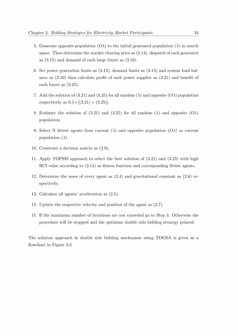
Chapter 3. Bidding Strategies for Electricity Market Participants 34
5. Generate opposite population (Oλ) to the initial generated population (λ) in search
space. Then determine the market clearing price as (3.14), dispatch of each generator
as (3.15) and demand of each large buyer as (3.16).
6. Set power generation limits as (3.12), demand limits as (3.13) and system load bal-
ance as (3.10) then calculate profit of each power supplier as (3.21) and benefit of
each buyer as (3.25).
7. Add the solution of (3.21) and (3.25) for all random (λ) and opposite (Oλ) population
respectively as 0.5 ∗ [(3.21) + (3.25)].
8. Evaluate the solution of (3.21) and (3.25) for all random (λ) and opposite (Oλ)
population.
9. Select N fittest agents from current (λ) and opposite population (Oλ) as current
population (λ).
10. Construct a decision matrix as (2.9).
11. Apply TOPSIS approach to select the best solution of (3.21) and (3.25) with high
RCI value according to (2.14) as fitness function and corresponding fittest agents.
12. Determine the mass of every agent as (2.4) and gravitational constant as (2.6) re-
spectively.
13. Calculate all agents’ acceleration as (2.5).
14. Update the respective velocity and position of the agent as (2.7).
15. If the maximum number of iterations are not exceeded go to Step 3. Otherwise the
procedure will be stopped and the optimum double side bidding strategy printed.
The solution approach in double side bidding mechanism using TOGSA is given as a
flowchart in Figure 3.2
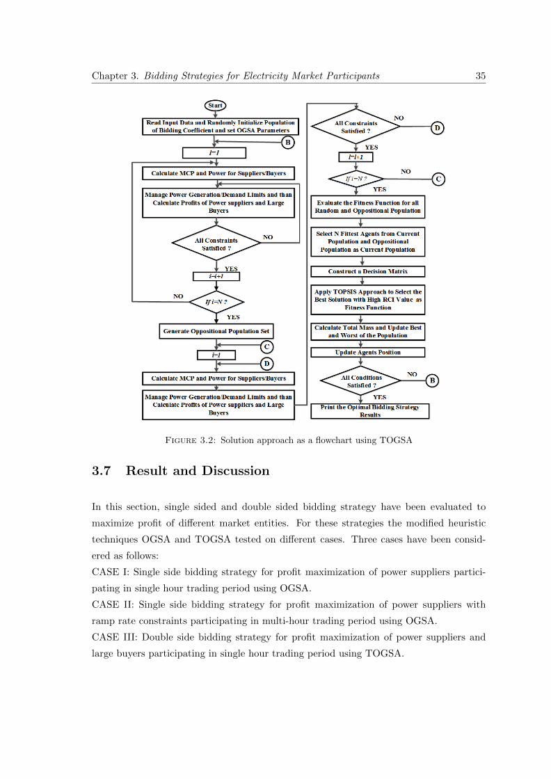
Chapter 3. Bidding Strategies for Electricity Market Participants 35
Figure 3.2: Solution approach as a flowchart using TOGSA
3.7 Result and Discussion
In this section, single sided and double sided bidding strategy have been evaluated to
maximize profit of different market entities. For these strategies the modified heuristic
techniques OGSA and TOGSA tested on different cases. Three cases have been consid-
ered as follows:
CASE I: Single side bidding strategy for profit maximization of power suppliers partici-
pating in single hour trading period using OGSA.
CASE II: Single side bidding strategy for profit maximization of power suppliers with
ramp rate constraints participating in multi-hour trading period using OGSA.
CASE III: Double side bidding strategy for profit maximization of power suppliers and
large buyers participating in single hour trading period using TOGSA.

Chapter 3. Bidding Strategies for Electricity Market Participants 36
3.7.1 CASE I
In this case, single side bidding strategy for profit maximization of power suppliers partic-
ipating in single hour trading period is tested on IEEE 30-bus system with inelastic load
demand 500 MW and solved by using OGSA. The generator data for IEEE 30-bus system
is given in Table A.1 and taken from [11]. The results obtained using OGSA are com-
pared to that of GSA , PSO [17] and binary coded GA method [22]. Also the results are
compared with the Monte Carlo (MC) method [11]. The tuning parameters of proposed
OGSA, GSA, PSO [17], and GA [22] methods are given in Table A.2. The simulation
results are carried out in MATLAB 2012a on a 3.20 GHz, i5 processor, 4GB RAM PC.
The considered value of coefficient αm,t is kept fixed as am,t and given in Table 3.1.
The optimal values of bidding coefficients βm,t is searched from the interval between
[bm,t M × bm,t] and M is set to be 5. The optimum values of βm,t for different genera-
tors using proposed OGSA, GSA, PSO [17], GA [22] and MC [11] are given in Table 3.1.
Table 3.1: Optimal bidding coefficients of power suppliers
PSs αm,tβm,t
MC [11] GA [22] PSO [17] GSA OGSA
1 2.00 0.158000 0.001045 0.001092 0.021004 0.026329
2 1.75 0.047450 0.048786 0.050953 0.090472 0.126153
3 1.00 0.130990 0.174234 0.181976 0.263500 0.352013
4 3.25 0.024580 0.023250 0.024283 0.054320 0.058808
5 3.00 0.056140 0.069694 0.072791 0.108594 0.157844
6 3.00 0.056140 0.069694 0.072791 0.108594 0.147336
Using the optimum bidding coefficients given in Table 3.1, the optimal bidding strategies
like market clearing price (MCP), individual generator power and profits using proposed
OGSA, GSA, PSO [17], GA [22] and MC [11] are shown in Table 3.2.
Table 3.2: Optimal bidding results for power suppliers
PSsMC [11] GA [22] PSO [17] GSA OGSA
PG Profit PG Profit PG Profit PG Profit PG Profit(MW) ($) (MW) ($) (MW) ($) (MW) ($) (MW) ($)
1 160 557 160 741.45 160 772.41 160 959.38 160 978.23
2 91.3 249 101.2 321.32 100.83 340.10 99.67 417.85 77.18 433.22
3 38.8 103 32.67 119.33 32.35 125.06 38.83 167.06 43.89 218.17
4 100 200 100 261.01 100 280.36 98.42 441.38 100 462.99
5 54.90 94 53 125.56 53.40 136.32 51.53 221.99 58.17 247.80
6 54.90 94 53 125.56 53.40 136.32 51.53 221.99 60.76 257.87
MCP ($/MW) 6.08 6.69 6.88 8.59 8.71
TP ($) 1297 1694.23 1790.57 2429.65 2595.28
TPG (MW) 499.99 499.99 499.99 499.99 500
From Table 3.2, it is noted that the total profit (TP) obtained using OGSA is higher than
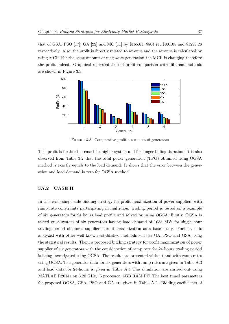
Chapter 3. Bidding Strategies for Electricity Market Participants 37
that of GSA, PSO [17], GA [22] and MC [11] by $165.63, $804.71, $901.05 and $1298.28
respectively. Also, the profit is directly related to revenue and the revenue is calculated by
using MCP. For the same amount of megawatt generation the MCP is changing therefore
the profit indeed. Graphical representation of profit comparison with different methods
are shown in Figure 3.3.
Figure 3.3: Comparative profit assessment of generators
This profit is further increased for higher system and for longer biding duration. It is also
observed from Table 3.2 that the total power generation (TPG) obtained using OGSA
method is exactly equals to the load demand. It shows that the error between the gener-
ation and load demand is zero for OGSA method.
3.7.2 CASE II
In this case, single side bidding strategy for profit maximization of power suppliers with
ramp rate constraints participating in multi-hour trading period is tested on a example
of six generators for 24 hours load profile and solved by using OGSA. Firstly, OGSA is
tested on a system of six generators having load demand of 1033 MW for single hour
trading period of power suppliers’ profit maximization as a base study. Further, it is
analyzed with other well known established methods such as GA, PSO and GSA using
the statistical results. Then, a proposed bidding strategy for profit maximization of power
supplier of six generators with the consideration of ramp rate for 24 hours trading period
is being investigated using OGSA. The results are presented without and with ramp rates
using OGSA. The generator data for six generators with ramp rates are given in Table A.3
and load data for 24-hours is given in Table A.4 The simulation are carried out using
MATLAB R2014a on 3.20 GHz, i5 processor, 4GB RAM PC. The best tuned parameters
for proposed OGSA, GSA, PSO and GA are given in Table A.2. Bidding coefficients of

Chapter 3. Bidding Strategies for Electricity Market Participants 38
power suppliers are calculated similarly as explained in CASE I. Only the value of M is
changed to 10 in this case. This assumption is kept unchanged for single and 24 hours.
Here, the optimal bidding strategy for system of six generators with load demand of
1033 MW is investigated using proposed OGSA, standard GSA, PSO and GA in single
hour trading period for power suppliers profit maximization. The MCP and net profits
evaluated at corresponding optimal bidding coefficients as given in Table 3.3 obtained using
GA, PSO, GSA and OGSA are 5.35 $/MW, 5.43 $/MW, 5.46 $/MW, 5.48 $/MW and $
1265.21, $ 1328.61, $ 1362.6, $ 1394.67 respectively. The optimal coefficient values and net
profit using proposed OGSA and other methods for comparison are presented in Table 3.3
and Table 3.4 respectively. It can be observed from the Table 3.4, that OGSA is getting
higher MCP and highest profit amongst all the methods. This proves the effectiveness of
OGSA in terms of results.
Table 3.3: Optimal bidding coefficients of power suppliers for single hour trading period
PSs αm,tβm,t
GA PSO GSA OGSA
1 4.10 0.003359 0.003409 0.003440 0.003539
2 4.50 0.034909 0.018594 0.021818 0.035696
3 4.10 0.005428 0.005616 0.005368 0.005467
4 3.74 0.028061 0.038421 0.038694 0.035635
5 3.82 0.005037 0.006140 0.006722 0.006149
6 3.78 0.035641 0.030983 0.032325 0.040405
Table 3.4: Optimal bidding results for single hour trading period
PSsGA PSO GSA OGSA
PG Profit PG Profit PG Profit PG Profit(MW) ($) (MW) ($) (MW) ($) (MW) ($)
1 371.48 426.25 385.58 469.4 392.2 490.3 387.1 493.5
2 30 22.74 46.54 36.31 40.88 34.03 30 26.69
3 229.53 261.96 232.78 282.5 250.2 310.2 249.2 315.0
4 60 85.02 60 89.46 60 91.53 60 92.94
5 298.95 407.79 258.22 377.2 240.8 362.5 266.7 403.7
6 43.04 61.45 49.88 73.76 48.86 74.1 40 62.79
MCP 5.35 5.43 5.46 5.48
TP 1265.21 1328.61 1362.6 1394.67TPG 1033 1033 1033 1033
Further, to compare the algorithms robustness, the quality solutions of 100 trials for all
considered algorithms are obtained and presented in Table 3.5. It can be observed from
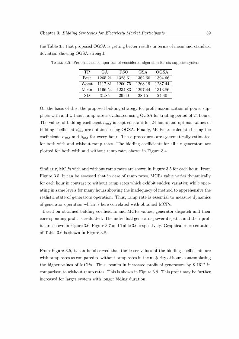
Chapter 3. Bidding Strategies for Electricity Market Participants 39
the Table 3.5 that proposed OGSA is getting better results in terms of mean and standard
deviation showing OGSA strength.
Table 3.5: Performance comparison of considered algorithm for six supplier system
TP GA PSO GSA OGSA
Best 1265.21 1328.61 1362.60 1394.66
Worst 1117.81 1200.75 1268.19 1287.44
Mean 1166.54 1234.83 1297.44 1313.86
SD 31.85 29.60 28.15 24.40
On the basis of this, the proposed bidding strategy for profit maximization of power sup-
pliers with and without ramp rate is evaluated using OGSA for trading period of 24 hours.
The values of bidding coefficient αm,t is kept constant for 24 hours and optimal values of
bidding coefficient βm,t are obtained using OGSA. Finally, MCPs are calculated using the
coefficients αm,t and βm,t for every hour. These procedures are systematically estimated
for both with and without ramp rates. The bidding coefficients for all six generators are
plotted for both with and without ramp rates shown in Figure 3.4.
Similarly, MCPs with and without ramp rates are shown in Figure 3.5 for each hour. From
Figure 3.5, it can be assessed that in case of ramp rates, MCPs value varies dynamically
for each hour in contrast to without ramp rates which exhibit sudden variation while oper-
ating in same levels for many hours showing the inadequacy of method to apprehensive the
realistic state of generators operation. Thus, ramp rate is essential to measure dynamics
of generator operation which is here correlated with obtained MCPs.
Based on obtained bidding coefficients and MCPs values, generator dispatch and their
corresponding profit is evaluated. The individual generator power dispatch and their prof-
its are shown in Figure 3.6, Figure 3.7 and Table 3.6 respectively. Graphical representation
of Table 3.6 is shown in Figure 3.8.
From Figure 3.5, it can be observed that the lesser values of the bidding coefficients are
with ramp rates as compared to without ramp rates in the majority of hours contemplating
the higher values of MCPs. Thus, results in increased profit of generators by $ 1612 in
comparison to without ramp rates. This is shown in Figure 3.9. This profit may be further
increased for larger system with longer biding duration.

Chapter 3. Bidding Strategies for Electricity Market Participants 40
(a) Values of βm,t for different generators with ramp rates
(b) Values of βm,t for different generators without ramp rates
Figure 3.4: Values of βm,t for different generators with and without ramp rates
Figure 3.5: Market clearing price (MCP) with and without ramp rates
3.7.3 CASE III
In this case, double side bidding strategy for profit maximization of power suppliers and
large buyers participating in single hour trading period is formulated as a multi-objective
problem. Formulated problem is tested on a system having six power suppliers and two
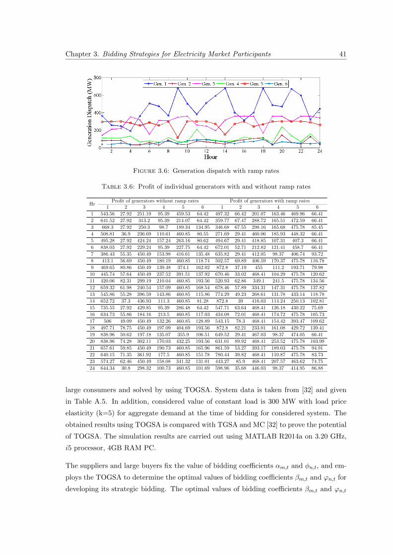
Chapter 3. Bidding Strategies for Electricity Market Participants 41
Figure 3.6: Generation dispatch with ramp rates
Table 3.6: Profit of individual generators with and without ramp rates
HrProfit of generators without ramp rates Profit of generators with ramp rates
1 2 3 4 5 6 1 2 3 4 5 6
1 543.56 27.92 251.19 95.39 459.53 64.42 497.32 66.42 201.07 163.46 469.96 66.41
2 641.52 27.92 313.2 95.39 214.07 64.42 359.77 67.47 288.72 165.51 472.59 66.41
3 668.3 27.92 250.3 98.7 189.34 134.95 346.68 67.55 298.16 165.68 475.78 85.45
4 508.81 36.9 236.69 110.61 460.85 80.55 271.69 29.41 460.06 185.93 448.32 66.41
5 495.28 27.92 424.24 157.24 263.16 80.62 494.67 29.41 418.85 107.31 407.3 66.41
6 838.03 27.92 229.24 95.39 227.75 64.42 672.01 52.71 212.82 121.41 458.7 66.41
7 386.43 55.35 450.49 153.98 416.61 135.48 635.82 29.41 412.05 98.37 406.74 93.72
8 413.1 56.69 450.49 180.19 460.85 118.74 502.57 69.89 406.59 170.37 475.78 116.78
9 469.65 80.86 450.49 139.48 374.1 162.02 872.8 37.19 455 111.2 193.71 79.98
10 445.74 57.64 450.49 237.52 391.51 137.92 670.46 33.02 468.41 104.29 475.78 120.62
11 420.06 82.31 299.19 210.04 460.85 193.56 520.93 62.86 349.1 241.5 475.78 134.56
12 659.32 61.98 240.54 157.09 460.85 168.54 678.46 57.89 334.31 147.31 475.78 137.82
13 545.86 55.28 396.59 143.86 460.85 115.86 774.29 49.23 268.61 131.78 433.14 118.78
14 652.72 37.3 436.93 111.3 460.85 81.28 872.8 39 416.03 114.24 250.13 102.81
15 735.55 27.92 429.85 95.39 286.48 64.42 547.71 63.64 468.41 126.18 430.22 75.69
16 634.73 55.86 184.16 213.5 460.85 117.03 434.08 72.01 468.41 174.72 475.78 105.73
17 506 49.09 450.49 132.26 460.85 128.89 543.15 78.3 468.41 154.42 393.47 109.62
18 497.71 78.75 450.49 197.09 404.69 193.56 872.8 82.21 233.01 161.08 429.72 139.41
19 838.96 50.62 197.18 135.07 355.9 106.51 649.52 29.41 467.03 98.37 474.05 66.41
20 838.96 74.28 302.11 170.03 432.25 193.56 631.01 89.92 468.41 253.52 475.78 103.99
21 657.61 59.85 450.49 190.73 460.85 165.96 861.59 53.27 393.17 189.03 475.78 94.91
22 640.15 71.35 361.92 177.5 460.85 151.78 780.44 39.82 468.41 110.87 475.78 83.73
23 574.27 62.46 450.49 158.08 341.32 131.01 443.27 85.9 468.41 207.57 463.62 74.75
24 644.34 30.8 298.32 100.73 460.85 101.69 598.96 35.68 446.03 98.37 414.95 86.88
large consumers and solved by using TOGSA. System data is taken from [32] and given
in Table A.5. In addition, considered value of constant load is 300 MW with load price
elasticity (k=5) for aggregate demand at the time of bidding for considered system. The
obtained results using TOGSA is compared with TGSA and MC [32] to prove the potential
of TOGSA. The simulation results are carried out using MATLAB R2014a on 3.20 GHz,
i5 processor, 4GB RAM PC.
The suppliers and large buyers fix the value of bidding coefficients αm,t and φn,t, and em-
ploys the TOGSA to determine the optimal values of bidding coefficients βm,t and ϕn,t for
developing its strategic bidding. The optimal values of bidding coefficients βm,t and ϕn,t

Chapter 3. Bidding Strategies for Electricity Market Participants 42
Figure 3.7: Generation dispatch without ramp rates
(a) Profit of individual generators for each hour with ramp rates
(b) Profit of individual generators for each hour without ramp rates
Figure 3.8: Profit of individual generators for each hour with and without ramp rates
is searched from the interval between [bm,t M × bm,t] and [fn,t M × fn,t] whereas
M is set to be 10 [32].
Considered system has been already investigated in strategic bidding problem considering
suppliers and buyers in [32]. Therefore, the proposed formulation has been firstly tested on
considered system and solved by using weighted sum method along with OGSA (WOGSA).
Figure 3.10 show that the weighted normalized solutions or Pareto-set for multi-objective

Chapter 3. Bidding Strategies for Electricity Market Participants 43
Figure 3.9: Comparative total profit assessment of generators with and without ramprates
strategic bidding problem using WOGSA for considered system. Pareto-set results provid-
Figure 3.10: Pareto-set for considered system using OGSA along with weighted summethod
ed by the solution for each objective is different for different weights. But the difficulty is
arising to find best results of individual objectives and best compromising results. There-
fore, TOPSIS technique is applied to find best compromising result. The optimal bidding
results of different suppliers/large buyers for considered system using WOGSA are pre-
sented in Table 3.7. Using the obtained optimal bidding coefficients αm,t, βm,t, φn,t and
ϕn,t as in Table 3.7, market clearing prices (MCP) are evaluated. The evaluated MCP
using WOGSA is higher than WGSA but lower than MC [32] approach. It is observed
from Table 3.7 that the overall profit of suppliers is increased by $463.29 using WOGSA as
compared to WGSA. On the other hand, overall profit can be further increased by $344.14
using MC [32] approach. However, the overall benefit of buyers using WOGSA and WGSA
[25] is increased by $ 158.6 and $ 225.9 as compared to MC [32] approach. WGSA also
seems more suitable for the buyers’ benefit.
In the light of above discussion authors concluded that the considered objectives are con-
tradictory in nature. The formulated problem cannot be handled as a true multi-objective

Chapter 3. Bidding Strategies for Electricity Market Participants 44
Table 3.7: Optimal bidding results for considered system using weighted sum methodalong with OGSA
PSs αm,t
MC [32] WGSA WOGSA
βm,tPG Profit
βm,tPG Profit
βm,tPG Profit
(MW) ($) (MW) ($) (MW) ($)
1 6.0 0.02927 160 1368 0.024071 160 1148.9 0.01905 160 1308.06
2 5.25 0.12420 89.4 572.7 0.485757 67.76 418.3 0.491757 77.6 516.14
3 3.0 0.29231 45.7 322.9 0.406048 67.27 183.74 1.144278 67.6 248.8
4 9.75 0.07433 88.8 386.4 0.124349 79.82 256.19 0.208625 77.44 330.24
5 9.0 0.17058 43.1 177.5 0.372618 57.76 95.22 0.50157 67.6 128.81
5 9.0 0.17058 43.1 177.5 0.620758 57.76 95.22 0.756491 67.6 128.81
Tot. 470.1 3005 490.37 2197.57 517.8 2660.86
LBs φn,t ϕn,tCD Benefit
ϕn,tCD Benefit
ϕn,tCD Benefit
(MW) ($) (MW) ($) (MW) ($)
1 30 0.09771 139.7 1126.3 0.075904 197.87 1405.78 0.094949 147.71 1198.8
2 25 0.07719 112.1 592.6 0.148658 67.4 539.02 0.037304 150 678.7
Tot. 251.8 1718.9 265.27 1944.8 297.71 1877.50
MCP 16.35 14.98 15.98
FD 218.3 225.1 220.12
TPT 470.1 490.37 517.8
T(P+B) 4723.1 4142.37 4538.36
optimization problem using weighted sum method. This limits the search capability for the
optimal solution. Thus, it becomes important for an algorithm to identify the overall opti-
mal operating point considering both entities (Suppliers and Buyers) together. Therefore,
TOPSIS technique is applied to find out the best compromising result. It is fundamentally
an effective method for multi-objective problem that decreases the Euclidean distance of
Pareto-set from best result of individual objects and provides best compromising solution.
Table 3.8: Optimal bidding results for considered system using TOPSIS along withOGSA
PSs αm,t
MC [32] TGSA TOGSA
βm,tPG Profit
βm,tPG Profit
βm,tPG Profit
(MW) ($) (MW) ($) (MW) ($)
1 6.0 0.02927 160 1368 0.037574 160 1386.6 0.053632 160 1391.8
2 5.25 0.12420 89.4 572.7 0.119268 114.2 596.2 0.143785 103.5 601.83
3 3.0 0.29231 45.7 322.9 0.449634 50.09 329.52 0.646152 46.15 330.11
4 9.75 0.07433 88.8 386.4 0.098465 88.35 395.73 0.030936 120 445.22
5 9.0 0.17058 43.1 177.5 0.673058 40.15 178.85 0.480586 45.26 185.75
6 9.0 0.17058 43.1 177.5 0.673058 40.15 178.85 0.480586 45.26 185.75
Tot. 470.1 3005 492.9 3065.7 520.2 3140.4
LBs φn,t ϕn,tCD Benefit
ϕn,tCD Benefit
ϕn,tCD Benefit
(MW) ($) (MW) ($) (MW) ($)
1 30 0.09771 139.7 1126.3 0.090492 149.6 1129.4 0.088446 152.7 1128.9
2 25 0.07719 112.1 592.6 0.067894 125.7 598.7 0.048842 150 600.2
Tot. 251.8 1718.9 275.3 1728.1 302.7 1729.1
MCP 16.35 16.47 16.50
FD 218.3 217.6 217.5
TPT 470.1 492.9 520.2
T(P+B) 4723.1 4793.8 4869.5

Chapter 3. Bidding Strategies for Electricity Market Participants 45
The optimal values of bidding coefficients αm,t, βm,t, φn,t and ϕn,t of different suppliers
and large buyers for considered system using TOPSIS along with OGSA (TOGSA) are
presented in Table 3.8. The evaluated MCP using TOGSA is higher than TGSA and
MC [32]. The MCP is proportionally related to profit through revenue. It is observed
from Table 3.8 that the overall profit of suppliers is increased using TOGSA as compared
to TGSA by $74.7 and MC [32] by $135.4. Also, the overall benefit of buyers using
TOGSA is increased as compared to TGSA by $1 and MC [32] by $10.2. TOGSA provides
an optimal MCP that maximizes the profit/benefit of suppliers/buyers. Thus, it further
encourages both entities to increase the trade of power. It is also observed from the
Table 3.8, that TOGSA results in 27.3 MW more power traded than TGSA and 50.1
MW as compared to MC [32]. The value of objective functions summation considering
double sided bidding using TOGSA is increased as compared to TGSA by $75.7 and
MC [32] by $145.5. Graphical representation of profit and benefit comparison of each
power supplier/large buyer with TOGSA, TGSA and MC [32] methods for considered
system is shown in Figure 3.11.
(a) Comparison of profit for individual power supplier
(b) Comparison of benefit for individual buyer
Figure 3.11: Profit and benefit comparison of each power supplier and large buyer forIEEE 30-bus system
Chapter 3. Bidding Strategies for Electricity Market Participants 46
3.8 Conclusions
In this chapter, two type of bidding strategy namely single and double side have been
evaluated for profit maximization of different market entities. Firstly, single side bidding
is tested in single and multi period with power balance and maximum/minimum generation
constraints. The ramp rate constraints is being considered in later part. After that double
side bidding strategy is investigated with same constraints as in former case.
Firstly, single side bidding strategy for profit maximization of power suppliers participating
in single hour trading period is solved using OGSA. The experimental outcomes in this
case shows that the proposed OGSA getting better results compared to other reported
techniques in terms of result quality. Then, in multi hour trading period with and without
ramp rate is solved using OGSA. The consideration of ramp rates provides practically
feasible values of generation dispatch off each unit and the results obtained clearly indicate
that the participation of generators in a day ahead electricity market bidding process
without considering ramp rate limits will cause economic loss to the generators as this
extra cost is beared by generators.
Secondly, double side bidding strategy for profit maximization of power suppliers and
large buyers participating in single hour trading period is formulated as a multi-objective
problem and solved by using TOGSA. In this problem, six power suppliers and two large
buyers have been considered in a day-ahead electricity market. The proposed techniques
are successful increasing the trading of power between suppliers and buyers and thus the
value of MCP and objective functions has been improved compared to other reported
techniques in terms of result quality. Moreover, the total power output of suppliers is
exactly equal to addition of the buyer’s demand and forecasted load demand.
The next Chapter exclusively has been devoted on bidding strategies with the inclusion
of renewable energy sources. In addition, uncertainties and limitations associated with
renewables have been modeled using an appropriate mathematical model for calculation
of market clearing price (MCP). This proposed approach is investigated on both single
and double side bidding mechanisms for a single hour trading period.
Chapter 4
Bidding Strategies for Electricity
Market Participants with
Amalgamation of Renewable
Power
4.1 Introduction
During the recent years, renewable energy sources (RESs) production plays a vital role in
moving towards a green economy. Due to this reason, RESs are under prime concern with
the annihilation of fossil fuels along with carbon emissions, which further draw the interest
of researchers [50]. As a part of the strategic bidding of conventional generators, the
GENCOs having renewable generation also participate in the bidding process. Electrical
power productions and percent of installed capacities of wind and solar power plants go
higher and will turn into the significant power generators soon [49]. This has led to the
new dimensions of exploration in optimal bidding strategy with amalgamation of wind and
solar based power generation. The main disadvantage of wind and solar power production
is its uncertainty and unpredictable nature of wind speed and solar irradiation which
always results in deviation from the actual generation. In the deregulated environment, the
uncertainty of wind and solar power has increased the problems manifold for the producers
in devising an optimal bidding strategy with CPS. Therefore in this chapter, optimum
bidding strategies such as single sided for power supplier and double sided for power
suppliers and large buyer have been formulated with amalgamation of substantial wind
47

Chapter 4. Bidding Strategies for Electricity Market Participants with Amalgamation ofRenewable Power 48
and solar based power generation. Moreover, the wind and solar are used as probabilistic
manner to model the uncertainty and their prediction error are considered in cost function
using underestimation and overestimation.
4.2 Modeling of Renewable Power Sources
In this section, modeling of solar irradiation and wind speed is elaborated. Solar irradiation
is modeled using Beta Probability Distribution Function (BPDF) and wind speed is mod-
eled through Weibull Probability Distribution Function (WPDF). The power probability
distributions obtained from respective models are used in further simulations.
4.2.1 Modeling of wind power
To build the optimal strategic bidding in the presence of wind power, handling of uncer-
tainty associated with wind speed has required. Data for wind speed at the considered
location of Barnstable city, MA, USA, follow a WPDF. The WPDF is given by [87,88] as
WPDF =k
c
(vc
)(k−1)(exp(−vc
)k)(4.1)
Wind speed characteristics depend on different factors such as, topography, geography etc.
The reasonable frequency of wind speed in the target zone can be used for calculation [88].
There are different strategies accessible in the literature to assess Weibull parameters. The
graphical technique for k and c estimation utilizing mean of historical wind speed (µhws)
and standard deviation (σstd) [89] as follows
k =
(σstdµhws
)(−1.086)
(4.2)
c =
µhws
Γ(
1 +(
1/k
)) (4.3)
Historical information about the speed of the wind, as estimated by anemometers intro-
duced at different heights in wind farms, is utilized in the generation of scenarios. Here,
first, 1000 scenarios are generated randomly by using WPDF and these generated scenar-
ios are changed over into power scenarios considering the hub heights. This procedure is
fundamental because the hub heights of introduced turbines and anemometers’ height are

Chapter 4. Bidding Strategies for Electricity Market Participants with Amalgamation ofRenewable Power 49
not the same in some situations [90]. This procedure has communicated as
v (hest) = v (hrkh)
(hghkah
)(γ)
(4.4)
The generated scenarios for the preferred height of the hub are converting into power
scenarios by utilizing the power curve for the measured model of wind turbine. The power
calculation can be represented as
Wa (v) =
0 v ≤ vin12ηp (v) ρAsv
3 vin ≤ v ≤ vrWr vr ≤ v ≤ vo0 v ≥ vo
(4.5)
Equation (4.5) demonstrates the production of random and distinct wind power variables.
Henceforth, it is essential to convert the distribution of available wind speed in terms of
power to be utilized in the future. The probability of the linear part [88] in wind power
output is defined as
fw (vin ≤ v ≤ vr) =
(kzvincWr
)[(1 + zWa/Wr)vin
c
]×
{−[
(1 + zWa/Wr)vinc
]k}(4.6)
Here, z is defined as z = (vr−vin)vin
The probability of zero wind power output [88] is represented as
fw [(v ≤ vin) and (v ≥ vo)] = 1− exp
[−(vinc
)k]+ exp
[−(voc
)k](4.7)
The probability of maximum (rated) wind power output [88] is defined as
fw(vr ≤ v ≤ vo) = exp
[−(vrc
)k]+ exp
[−(voc
)k](4.8)
4.2.2 Modeling of Solar Power
It is necessary to handle the uncertainty associated with solar irradiation in order to deal
with strategic bidding in the presence of solar power. Conversion of the solar irradiations
is usually dependent upon the solar cell temperature, insolation of solar and technical
properties of different PV modules. The output of solar power can be calculated by using
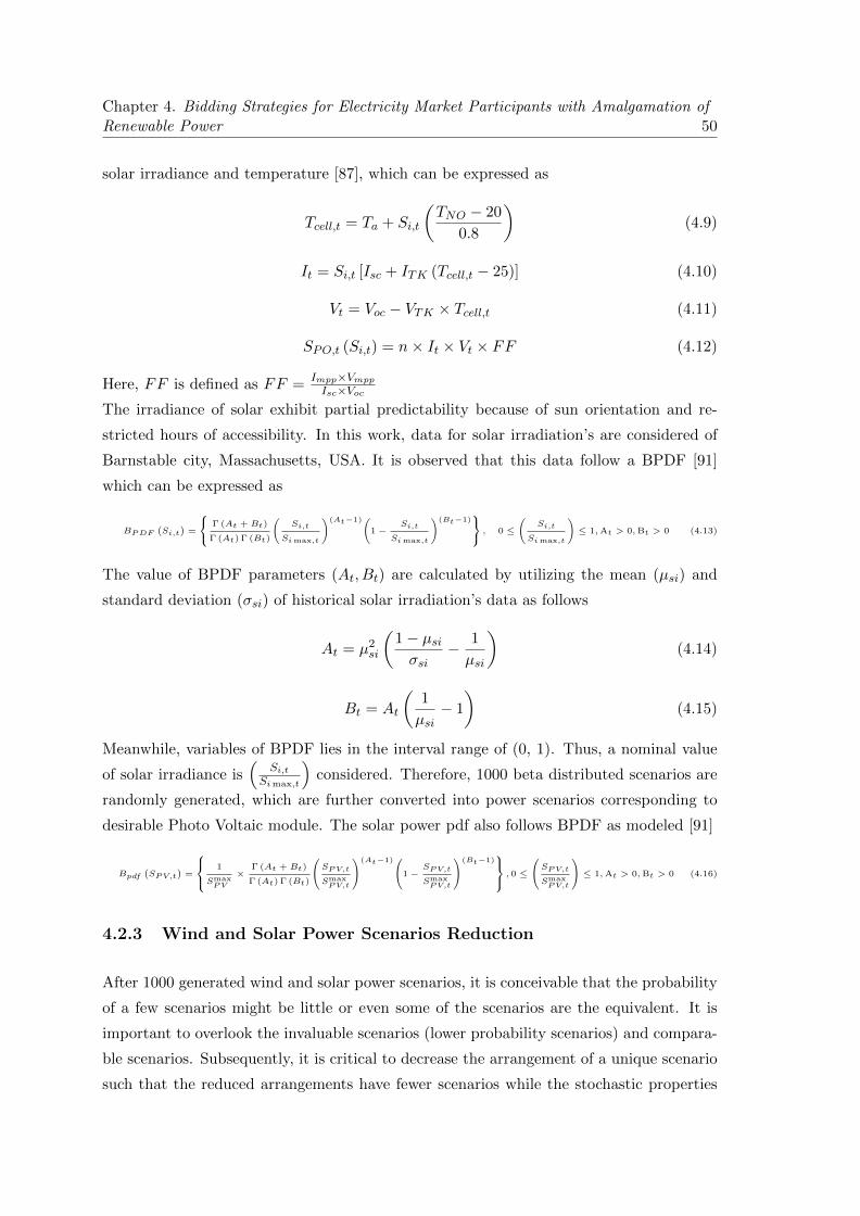
Chapter 4. Bidding Strategies for Electricity Market Participants with Amalgamation ofRenewable Power 50
solar irradiance and temperature [87], which can be expressed as
Tcell,t = Ta + Si,t
(TNO − 20
0.8
)(4.9)
It = Si,t [Isc + ITK (Tcell,t − 25)] (4.10)
Vt = Voc − VTK × Tcell,t (4.11)
SPO,t (Si,t) = n× It × Vt × FF (4.12)
Here, FF is defined as FF =Impp×VmppIsc×Voc
The irradiance of solar exhibit partial predictability because of sun orientation and re-
stricted hours of accessibility. In this work, data for solar irradiation’s are considered of
Barnstable city, Massachusetts, USA. It is observed that this data follow a BPDF [91]
which can be expressed as
BPDF(Si,t
)=
Γ (At + Bt)
Γ (At) Γ (Bt)
(Si,t
Simax,t
)(At−1)(1−
Si,t
Simax,t
)(Bt−1) , 0 ≤
(Si,t
Simax,t
)≤ 1,At > 0,Bt > 0 (4.13)
The value of BPDF parameters (At, Bt) are calculated by utilizing the mean (µsi) and
standard deviation (σsi) of historical solar irradiation’s data as follows
At = µ2si
(1− µsiσsi
− 1
µsi
)(4.14)
Bt = At
(1
µsi− 1
)(4.15)
Meanwhile, variables of BPDF lies in the interval range of (0, 1). Thus, a nominal value
of solar irradiance is(
Si,tSimax,t
)considered. Therefore, 1000 beta distributed scenarios are
randomly generated, which are further converted into power scenarios corresponding to
desirable Photo Voltaic module. The solar power pdf also follows BPDF as modeled [91]
Bpdf(SPV,t
)=
1
SmaxPV
×Γ (At + Bt)
Γ (At) Γ (Bt)
SPV,t
SmaxPV,t
(At−1)1−SPV,t
SmaxPV,t
(Bt−1) , 0 ≤
SPV,t
SmaxPV,t
≤ 1,At > 0,Bt > 0 (4.16)
4.2.3 Wind and Solar Power Scenarios Reduction
After 1000 generated wind and solar power scenarios, it is conceivable that the probability
of a few scenarios might be little or even some of the scenarios are the equivalent. It is
important to overlook the invaluable scenarios (lower probability scenarios) and compara-
ble scenarios. Subsequently, it is critical to decrease the arrangement of a unique scenario
such that the reduced arrangements have fewer scenarios while the stochastic properties

Chapter 4. Bidding Strategies for Electricity Market Participants with Amalgamation ofRenewable Power 51
are not changed importantly. The quantity of diminished scenarios relies on the sort and
nature of the issue to be optimized, and it must be short of what one-fourth of generated
scenarios [90].
The primary objective of scenario reduction techniques is to eliminate the scenarios with
low and same probabilities. In this manner, a subset of scenarios of their new probabilities
are evaluated such that probability measure of reduced scenarios should remain close to
the main probability measure in terms of probability distance between two probabilities.
The scenario decrease technique minimizes and packages the scenarios, utilizing the Kan-
torovich Distance Matrix (KDM) [90], [92]. KD is the distance of probabilities between
two different scenario arrangements that express a similar stochastic process. It is used to
consider the closeness of various scenario arrangements for most part. KD guarantees that
most extreme conceivable scenarios are decreasing without damaging a given resilience
rule. The probability of all decreased scenarios are supposed to be zero. The new prob-
ability of ensured scenario is equivalent to the total of its previous probability and the
probability of removed scenarios that are nearest to it. In KD technique, the following
steps are used to scenarios reduction.
1. The KD is calculated for every combination of scenarios and create the KDM con-
taining entire scenarios and relative distance to one another. The estimation of the
distance between two scenarios υi and υj are given by
KD(υi, υj
)=
(ηl∑l=0
(vil − v
jl
)2) 1
2
(4.17)
2. Find a different closest scenario for every scenario υi, namely the scenario υj , j 6= i
of the minimum KD to asses scenario min{KD
(υi, υj
)}. The recognized scenario
can be effortlessly set apart in the KDM.
3. Corresponding to each combination of scenarios obtained in Step 2, calculate
min{KD
(υi, υj
)}× P
[υi]
(4.18)
Next, the qualities for entire scenario sets are analyzed in KDM and the least im-
portant sets are identified. From two individuals of this set, the scenario which will
be removed first is selected depending on the following conditions:
(a) Comparative nearness to different scenarios too.
(b) Low probability of occurrence.
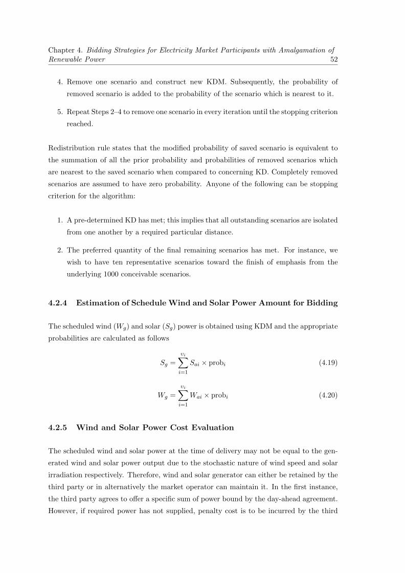
Chapter 4. Bidding Strategies for Electricity Market Participants with Amalgamation ofRenewable Power 52
4. Remove one scenario and construct new KDM. Subsequently, the probability of
removed scenario is added to the probability of the scenario which is nearest to it.
5. Repeat Steps 2–4 to remove one scenario in every iteration until the stopping criterion
reached.
Redistribution rule states that the modified probability of saved scenario is equivalent to
the summation of all the prior probability and probabilities of removed scenarios which
are nearest to the saved scenario when compared to concerning KD. Completely removed
scenarios are assumed to have zero probability. Anyone of the following can be stopping
criterion for the algorithm:
1. A pre-determined KD has met; this implies that all outstanding scenarios are isolated
from one another by a required particular distance.
2. The preferred quantity of the final remaining scenarios has met. For instance, we
wish to have ten representative scenarios toward the finish of emphasis from the
underlying 1000 conceivable scenarios.
4.2.4 Estimation of Schedule Wind and Solar Power Amount for Bidding
The scheduled wind (Wg) and solar (Sg) power is obtained using KDM and the appropriate
probabilities are calculated as follows
Sg =
υi∑i=1
Sai × probi (4.19)
Wg =
υi∑i=1
Wai × probi (4.20)
4.2.5 Wind and Solar Power Cost Evaluation
The scheduled wind and solar power at the time of delivery may not be equal to the gen-
erated wind and solar power output due to the stochastic nature of wind speed and solar
irradiation respectively. Therefore, wind and solar generator can either be retained by the
third party or in alternatively the market operator can maintain it. In the first instance,
the third party agrees to offer a specific sum of power bound by the day-ahead agreement.
However, if required power has not supplied, penalty cost is to be incurred by the third

Chapter 4. Bidding Strategies for Electricity Market Participants with Amalgamation ofRenewable Power 53
party. In this work, later case has considered, in which the wind and solar generators are
claimed by the market operator, and in this way, there will be no cost incurred in terms
of penalty.
However, when there is an overestimation of wind power, either power is purchased from
exchange sources, or load shedding is carried out to keep the power balance, then the same
amount is reflected in terms of penalty addressing both economic and reliability concerns.
Also, in case of wind and solar power underestimation, wind and solar generators need to
decrease the produced power along these lines which results in wastage of available power
limit and adverse impact on the environmental conditions [87]. Therefore, both these cir-
cumstances are contrary (one leans toward more reliance on wind and solar generators for
power needs though alternate empowers the utilization of something beyond solid conven-
tional generators) and also detrimental from the perspective of economy, environment, and
reliability of operation. The condition of mismatch can be incorporated as imbalance term
in cost function when wind and solar generation are owned by the system operator. This
imbalance cost of wind and solar measures the difference in forecasted and actual power,
which is summation of underestimation and overestimation cost. It can be expressed as
IMC(Wgn) = Oc(wg) + Uc(wg) (4.21)
IMC(Sgn) = Oc(Sg) + Uc(Sg) (4.22)
Here, it should be noted that condition of overestimation of wind power is more harmful
as compared to underestimation of wind power. The evaluation of overestimation and
underestimation cost of available wind and solar power are as follows:
4.2.5.1 Estimation of Overestimation Cost for Available Wind and Solar Pow-
er
The deficit in power is a decisive factor in evaluating the cost of overestimation of solar and
wind power. The probability of this shortage incidence for a specified amount of scheduled
solar and wind power is formulated as
Oc(wg) = Ko ×Wg∫0
(Wg −Wa)× fWa(Wa)× dWa (4.23)
Oc(Sg) = Ko ×Sg∫0
(Sg − Sa)× fSa(Sa)× dSa (4.24)
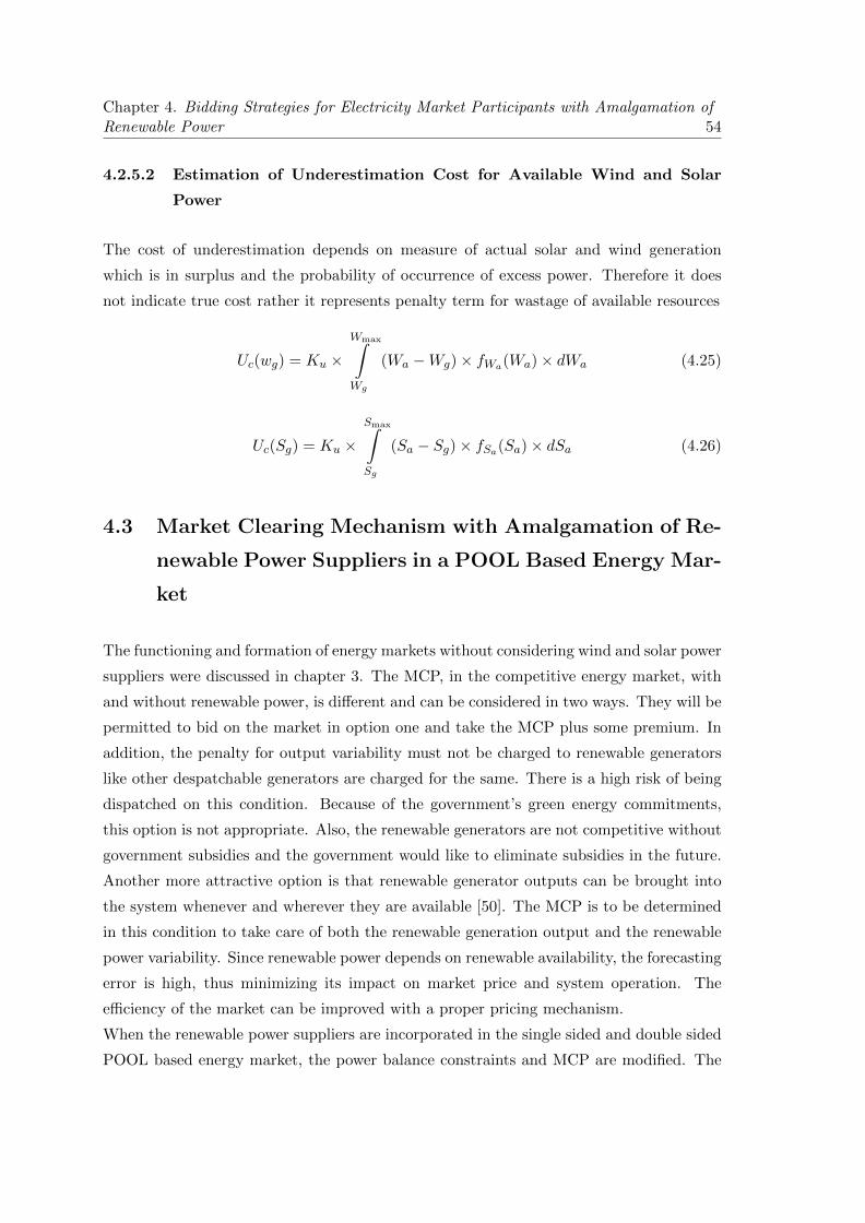
Chapter 4. Bidding Strategies for Electricity Market Participants with Amalgamation ofRenewable Power 54
4.2.5.2 Estimation of Underestimation Cost for Available Wind and Solar
Power
The cost of underestimation depends on measure of actual solar and wind generation
which is in surplus and the probability of occurrence of excess power. Therefore it does
not indicate true cost rather it represents penalty term for wastage of available resources
Uc(wg) = Ku ×Wmax∫Wg
(Wa −Wg)× fWa(Wa)× dWa (4.25)
Uc(Sg) = Ku ×Smax∫Sg
(Sa − Sg)× fSa(Sa)× dSa (4.26)
4.3 Market Clearing Mechanism with Amalgamation of Re-
newable Power Suppliers in a POOL Based Energy Mar-
ket
The functioning and formation of energy markets without considering wind and solar power
suppliers were discussed in chapter 3. The MCP, in the competitive energy market, with
and without renewable power, is different and can be considered in two ways. They will be
permitted to bid on the market in option one and take the MCP plus some premium. In
addition, the penalty for output variability must not be charged to renewable generators
like other despatchable generators are charged for the same. There is a high risk of being
dispatched on this condition. Because of the government’s green energy commitments,
this option is not appropriate. Also, the renewable generators are not competitive without
government subsidies and the government would like to eliminate subsidies in the future.
Another more attractive option is that renewable generator outputs can be brought into
the system whenever and wherever they are available [50]. The MCP is to be determined
in this condition to take care of both the renewable generation output and the renewable
power variability. Since renewable power depends on renewable availability, the forecasting
error is high, thus minimizing its impact on market price and system operation. The
efficiency of the market can be improved with a proper pricing mechanism.
When the renewable power suppliers are incorporated in the single sided and double sided
POOL based energy market, the power balance constraints and MCP are modified. The

Chapter 4. Bidding Strategies for Electricity Market Participants with Amalgamation ofRenewable Power 55
rest equations and procedure will remain same as described in chapter 3. The modified
power balance constraints, MCP and objective functions are represented as
1. Power balance constraints
(a) Single SideCPS,T∑m=1,t=1
PGm,t +
RPS,T∑x=1,t=1
RGx,t = D (Rs,t) (4.27)
(b) Double Side
CPS,T∑m=1,t=1
PGm,t +
RPS,T∑x=1,t=1
RGx,t = D (Rd,t) +
LB,T∑n=1,t=1
CDn,t (4.28)
2. MCPs
(a) Single Side
Rs,t =
Dc,t −RPS,T∑x=1,t=1
RGx,t +CPS,T∑m=1,t=1
αm,tβm,t
K +CPS,T∑m=1,t=1
1βm,t
(4.29)
(b) Double Side
Rd,t =
Dc,t −RPS,T∑x=1,t=1
RGx,t +CPS,T∑m=1,t=1
αm,tβm,t
+LB,T∑
n=1,t=1
φm,tϕm,t
K +CPS,T∑m=1,t=1
1βm,t
+LB,T∑
n=1,t=1
1ϕn,t
(4.30)
4.4 Problem Formulation in Single Side POOL Based Ener-
gy Market with Amalgamation of Renewable Power
With amalgamation of renewable power, the objective function for profit maximization of
market participants in single side POOL based energy market is modified as
Maximize
FS(αm,t, βm,t) = Rs,t×PGm,t+Rs,t×RGx,t−PCSm,t(PGSm,t)− IMCx,t(RGx,t) (4.31)
Subject to: Power balance constraints as given in equation (4.27), power inequality con-
straints as given in equation (3.4) and renewable power constraints as given in equations
(4.21) and (4.22).

Chapter 4. Bidding Strategies for Electricity Market Participants with Amalgamation ofRenewable Power 56
4.5 Problem Formulation in Double Side POOL Based En-
ergy Market with Amalgamation of Renewable Power
With amalgamation of renewable power, the objective function for profit maximization of
market participants in double side POOL based energy market is modified as
Maximizes
FD(αm,t, βm,t) = Rd,t × PGDm,t +Rd,t ×RGx,t − PCDm,t(PGDm,t)− IMCx,t(RGx,t)
(4.32)
FD(φn,t, ϕn,t) = PCDn,t(CDn,t)−Rd,t × CDn,t (4.33)
Subject to: Power balance constraints as given in equation (4.28), power and demand
inequality constraints as given in equations (3.12) and (3.13), and renewable power con-
straints as given in equations (4.21) and (4.22).
The bid data of the rivals and their corresponding joint normal PDFs are estimated same
as described in chapter 3. The proposed OGSA and TOGSA are respectively applied to
solve the above stochastic single and double side optimization problem with amalgamation
of renewable power.
4.6 Solution Methodology
4.6.1 Solution Procedure of OGSA Applied to Single Side Optimal Bid-
ding Strategy problem with Amalgamation of Renewable Power
1. Set input data of considered test system, Wind and solar data as discussed in mod-
eling of renewable power sources for single side bidding strategy and parameters of
the proposed OGSA.
2. Set population size (N) and randomly generate initial population λ for bidding co-
efficient βm,t of power suppliers in the decided search space of the problem.
3. Determine the market clearing price as (4.29) and dispatch of each generator as (3.7).
4. Set power generation limits as (3.4) and system load balance as (4.27) then calculate
profit of each power supplier as (4.31).
5. Generate opposite population (Oλ) to the initial generated population (λ) in search
space. Then determine the market clearing price as (4.29) and dispatch of each
generator as (3.7).

Chapter 4. Bidding Strategies for Electricity Market Participants with Amalgamation ofRenewable Power 57
6. Set power generation limits as (3.4) and system load balance as (4.27) then calculate
profit of each power supplier as (4.31).
7. Evaluate the fitness function for all random (λ) and opposite (Oλ) population.
8. Select N fittest agents from current (λ) and opposite population (Oλ) as current
population (λ).
9. Determine the mass of every agent as (2.4) and gravitational constant as (2.6) re-
spectively.
10. Calculate all agents’ acceleration as (2.5).
11. Update the respective velocity and position of the agent as (2.7).
12. If the maximum number of iterations are not exceeded go to Step 3, otherwise
the procedure will be stopped and the optimum single side bidding strategy with
amalgamation of wind power printed.
4.6.2 Solution Procedure of TOGSA Applied to Double Side Optimal
Bidding Strategy Problem with Amalgamation of Renewable Pow-
er
1. Set input data of considered test system for double side bidding strategy and pa-
rameters of the proposed TOGSA.
2. Set population size (N) and randomly generate initial population λ for bidding co-
efficient βm,t of power suppliers in the decided search space of the problem.
3. Determine the market clearing price as (4.30), dispatch of each generator as (3.15)
and demand of each large buyer as (3.16).
4. Set power generation limits as (3.12), demand limits as (3.13) and system load bal-
ance as (4.28) then calculate profit of each power supplier as (4.31) and benefit of
each buyer as (4.32).
5. Generate opposite population (Oλ) to the initial generated population (λ) in search
space. Then determine the market clearing price as (4.30), dispatch of each generator
as (3.15) and demand of each large buyer as (3.16).
6. Set power generation limits as (3.12), demand limits as (3.13) and system load bal-
ance as (4.28) then calculate profit of each power supplier as (4.31) and benefit of
each buyer as (4.32).

Chapter 4. Bidding Strategies for Electricity Market Participants with Amalgamation ofRenewable Power 58
7. Add the solution of (4.31) and (4.32) for all random (λ) and opposite (Oλ) population
respectively as 0.5 ∗ [(3.21) + (3.25)].
8. Evaluate the solution of (4.31) and (4.32) for all random (λ) and opposite (Oλ)
population.
9. Select N fittest agents from current (λ) and opposite population (Oλ) as current
population (λ).
10. Construct a decision matrix as (2.9).
11. Apply TOPSIS approach to select the best solution of (4.31) and (4.32) with high
RCI value according to (2.14) as fitness function and corresponding fittest agents.
12. Determine the mass of every agent as (2.4) and gravitational constant as (2.6) re-
spectively.
13. Calculate all agents’ acceleration as (2.5).
14. Update the respective velocity and position of the agent as (2.7).
15. If the maximum number of iterations are not exceeded go to Step 3, otherwise
the procedure will be stopped and the optimum double side bidding strategy with
amalgamation of renewable power printed.
4.7 Result and Discussion
In this section, single sided and double sided bidding strategy with inclusion of renewable
energy sources have been evaluated to maximize profit of different market entities. A
modified heuristic technique, OGSA is used to solve single sided bidding strategy and
TOGSA is used to solve double sided bidding strategy. Three cases are considered as
follows
1. CASE I: Single sided bidding strategy with inclusion of only wind power using OGSA
in a single hour trading period.
2. Case II: Single sided bidding strategy with and without inclusion of only with wind,
only with solar and combination of both wind and solar power using OGSA in a
single hour trading period.
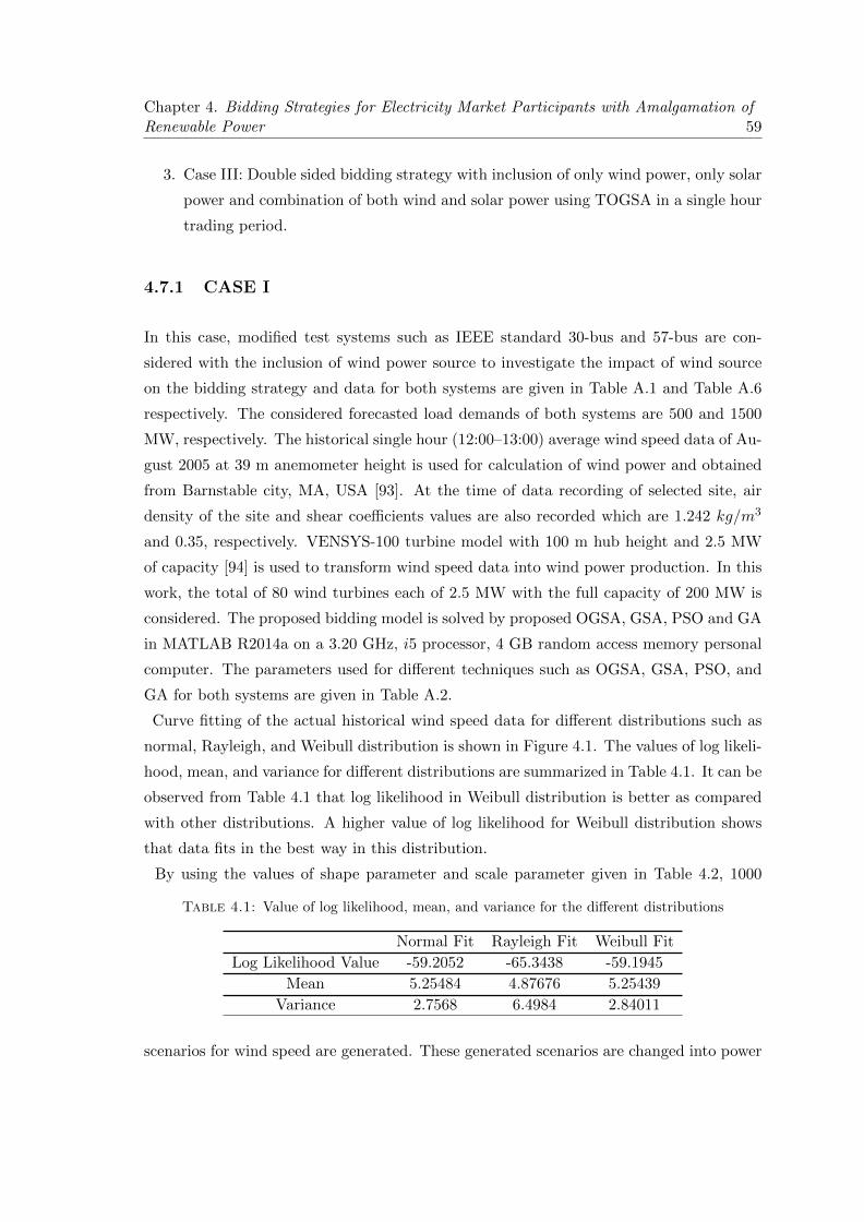
Chapter 4. Bidding Strategies for Electricity Market Participants with Amalgamation ofRenewable Power 59
3. Case III: Double sided bidding strategy with inclusion of only wind power, only solar
power and combination of both wind and solar power using TOGSA in a single hour
trading period.
4.7.1 CASE I
In this case, modified test systems such as IEEE standard 30-bus and 57-bus are con-
sidered with the inclusion of wind power source to investigate the impact of wind source
on the bidding strategy and data for both systems are given in Table A.1 and Table A.6
respectively. The considered forecasted load demands of both systems are 500 and 1500
MW, respectively. The historical single hour (12:00–13:00) average wind speed data of Au-
gust 2005 at 39 m anemometer height is used for calculation of wind power and obtained
from Barnstable city, MA, USA [93]. At the time of data recording of selected site, air
density of the site and shear coefficients values are also recorded which are 1.242 kg/m3
and 0.35, respectively. VENSYS-100 turbine model with 100 m hub height and 2.5 MW
of capacity [94] is used to transform wind speed data into wind power production. In this
work, the total of 80 wind turbines each of 2.5 MW with the full capacity of 200 MW is
considered. The proposed bidding model is solved by proposed OGSA, GSA, PSO and GA
in MATLAB R2014a on a 3.20 GHz, i5 processor, 4 GB random access memory personal
computer. The parameters used for different techniques such as OGSA, GSA, PSO, and
GA for both systems are given in Table A.2.
Curve fitting of the actual historical wind speed data for different distributions such as
normal, Rayleigh, and Weibull distribution is shown in Figure 4.1. The values of log likeli-
hood, mean, and variance for different distributions are summarized in Table 4.1. It can be
observed from Table 4.1 that log likelihood in Weibull distribution is better as compared
with other distributions. A higher value of log likelihood for Weibull distribution shows
that data fits in the best way in this distribution.
By using the values of shape parameter and scale parameter given in Table 4.2, 1000
Table 4.1: Value of log likelihood, mean, and variance for the different distributions
Normal Fit Rayleigh Fit Weibull Fit
Log Likelihood Value -59.2052 -65.3438 -59.1945
Mean 5.25484 4.87676 5.25439
Variance 2.7568 6.4984 2.84011
scenarios for wind speed are generated. These generated scenarios are changed into power

Chapter 4. Bidding Strategies for Electricity Market Participants with Amalgamation ofRenewable Power 60
Figure 4.1: Curve fitting of the historical single hour (1200-1300 hrs) wind speed dataof Barnstable city, MA, USA for different distributions
scenarios considering the desirable hub heights. After that probability of generated pow-
er scenarios is assigned by using Weibull distribution, then the probabilities associated
with generated power scenarios is normalized such that their summation is equal to uni-
ty. Weibull and normalize Weibull probabilities density for generated power scenarios are
shown in Figure 4.2.
A KDM method [90], [92] is used to reduce the scenarios for accurate modeling of wind
Table 4.2: Value of the shape parameter and the scale parameter of wind speed
Hub Height Shape Parameter Scale Parameter (m/s)
39 meter 3.49 5.84
100 meter 3.49 8.13
power uncertainty. This is performed as a large number of scenarios become quite cum-
bersome to model the uncertainty. Here, ten reduced scenarios are produced from 1000
generated scenarios. On the basis of these reduced scenarios, in the considered hour, wind
power is scheduled. The final KDM with wind power outputs and their probabilities for
reduced ten numbers of scenarios are given in Table 4.3. On the basis on wind power
outputs and their probabilities, probable assessment of wind power is calculated for that
hour. Probable value of wind power is 51.95 MW, considered as schedule wind power for
that hour. The summation of reduced scenarios probabilities is always equal to unity.
After that, the strategic bidding model with and without wind power is solved by using

Chapter 4. Bidding Strategies for Electricity Market Participants with Amalgamation ofRenewable Power 61
Figure 4.2: Weibull and normalize Weibull probability densities for generated powerscenarios of single hour (1200-1300 hrs) wind speed data of Barnstable city, MA, USA
Table 4.3: Final KDM with wind power outputs and their probabilities for reduced tennumbers of scenarios
Index 1 2 3 4 5 6 7 8 9 10 Wa (MW) Probability Min (KD)
1 0 18.09 44.3 70.87 92.94 111.1 126.1 145.3 167.7 180.7 10.56 0.142 18.09
2 18.09 0 26.22 52.78 74.85 93.04 108 127.2 149.6 162.6 28.65 0.283 18.09
3 44.3 26.22 0 26.57 48.63 66.83 81.82 101 123.4 136.4 54.86 0.325 26.22
4 70.87 52.78 26.57 0 22.07 40.26 55.25 74.4 96.83 109.8 81.43 0.144 22.07
5 92.94 74.85 48.63 22.07 0 18.19 33.19 52.33 74.76 87.76 103.5 0.049 18.19
6 111.1 93.04 66.83 40.26 18.19 0 14.99 34.14 56.57 69.56 121.7 0.029 14.99
7 126.1 108 81.82 55.25 33.19 14.99 0 19.15 41.58 54.57 136.7 0.013 14.99
8 145.3 127.2 101 74.4 52.33 34.14 19.15 0 22.43 35.42 155.8 0.01 19.15
9 167.7 149.6 123.4 96.83 74.76 56.57 41.58 22.43 0 12.99 178.3 0.002 12.99
10 180.7 162.6 136.4 109.8 87.76 69.56 54.57 35.42 12.99 0 191.2 0.002 12.99
proposed OGSA, GSA, PSO, and GA for both systems. In the process of strategic bid-
ding, the coefficients of bidding are not considered individually for maximization of profit
for conventional generators. Owing to the inter-dependency of bidding coefficients, the
values of one bidding coefficient considered as known values then values of other bidding
coefficient are determined by using an optimization method [11]. Therefore, in this work,
values of bidding coefficient αm,t is fixed and employ the proposed OGSA, GSA, GA, and
PSO to determine the optimum values of bidding coefficient βm,t from the search space
between [bm,t M × bm,t], M is set to be 10. The values of joint normal distribution
parameters for the suppliers are obtained from [11].
First, the optimum values of bidding coefficients for IEEE standard 30-bus are obtained
using proposed OGSA, GSA, PSO, and GA and given in Table 4.4. The optimal bidding
strategy to clear the MCP for the IEEE standard 30-bus system is calculated after deter-
mining the optimal bidding coefficients using proposed OGSA, GSA, PSO, and GA. The

Chapter 4. Bidding Strategies for Electricity Market Participants with Amalgamation ofRenewable Power 62
MCP and net profits evaluated at corresponding optimal bidding coefficients obtained us-
ing GA, PSO, GSA, and proposed OGSA are 12.55 $/MW, 12.89 $/MW, 13.9458 $/MW,
14.15 $/MW and $4490.02, $4672.93, $5212.6, $5317.72 respectively. From Table 4.4, it
can be observed that among all the algorithms, OGSA is getting highest MCP and net
profit. It can be shown that the OGSA is outperforming over both algorithms.
Similarly, for IEEE standard 57-bus system results are obtained and given in Table 4.5.
Table 4.4: Optimum bidding results for IEEE standard 30-bus
PSs αm,t
GA PSO GSA OGSAβm,t PG Profit βm,t PG Profit βm,t PG Profit βm,t PG Profit
(MW) ($) (MW) ($) (MW) ($) (MW) ($)
1 2.0 0.044090 160 1592.4 0.042666 160 1645.73 0.049231 160 1815.32 0.049984 160 1848.47
2 1.75 0.19429 75.05 712.19 0.211031 74.81 735.14 0.224134 77.45 839.65 0.223528 78.68 867.49
3 1.0 0.300167 57.94 459.54 0.436374 49.28 433.95 0.722945 40.95 425.33 0.680919 42.5 446.15
4 3.25 0.094465 100 846.85 0.103585 100 880.18 0.097653 100 986.18 0.099466 100 1006.9
5 3.0 0.280553 53.50 439.52 0.275273 57.95 488.96 0.289934 60.80 573.06 0.307913 59.41 574.36
6 3.0 0.280553 53.50 439.52 0.275273 57.95 488.96 0.289934 60.80 573.06 0.307913 59.41 574.36
MCP 12.55 12.89 13.9458 14.15
TP 4490.02 4672.93 5212.6 5317.72
TPG 500 500 500 500
From Table 4.5, it can be seen that obtained MCP and corresponding calculated net profit
at optimality using GA, PSO, GSA and proposed GSA are 12.19 $/MW, 12.35 $/MW,
12.87 $/MW, 12.97 $/MW and $13,244.65, $13,457.81, $14,065.79, $14077.77, respectively.
Now, to measure the effect of wind source is considered in the both IEEE standard 30-bus
Table 4.5: Optimum bidding results for IEEE standard 57-bus
PSs αm,t
GA PSO GSA OGSAβm,t PG Profit βm,t PG Profit βm,t PG Profit βm,t PG Profit
(MW) ($) (MW) ($) (MW) ($) (MW) ($)
1 1.7365 0.019718 530.23 5065.65 0.020393 520.21 5058.66 0.021819 510.26 5238.34 0.022239 505.16 5241.2
2 10 0.095015 23.07 45.23 0.098836 23.73 50.02 0.092598 30.99 79.34 0.076760 38.7 99.99
3 7.1429 0.078495 64.32 295.35 0.082602 62.98 299.48 0.081198 70.53 368.62 0.088860 65.58 351.7
4 10 0.095015 23.07 45.23 0.098836 23.73 50.02 0.092598 30.99 79.34 0.076760 38.7 99.99
5 1.81 0.020843 498.08 4724.32 0.021487 490.31 4732.82 0.02278 485.52 4945.47 0.023240 480.23 4944.7
6 10 0.095015 23.07 45.23 0.098836 23.73 50.02 0.092598 30.99 79.34 0.076760 38.7 99.99
7 2.4390 0.028839 338.18 3023.63 0.02788 355.31 3216.81 0.030615 340.71 3275.32 0.031635 332.92 3240.2
MCP 12.19 12.35 12.87 12.97
TP 13244.65 13457.81 14065.79 14077.77
TPG 1500 1500 1500 1500
and 57-bus systems and solved by using proposed OGSA, GSA, PSO, and GA successively.
For strategic bidding of wind power in the market is permitted by modifying the demand
and then by updating the bidding coefficients in agreement to new demand as suggested
in [50]. On the basis on this approach, MCP is calculated at modified demand, i.e. actual
demand minus wind power. In this work, the operational cost of the wind power generator
is not considered as it is justifiable to deliberate their imbalance cost due to uncertainty as-
sociated with wind generation. This is measured by the two components of imbalance cost
(overestimation and underestimation). This reflects on the net profit gained by wind PS
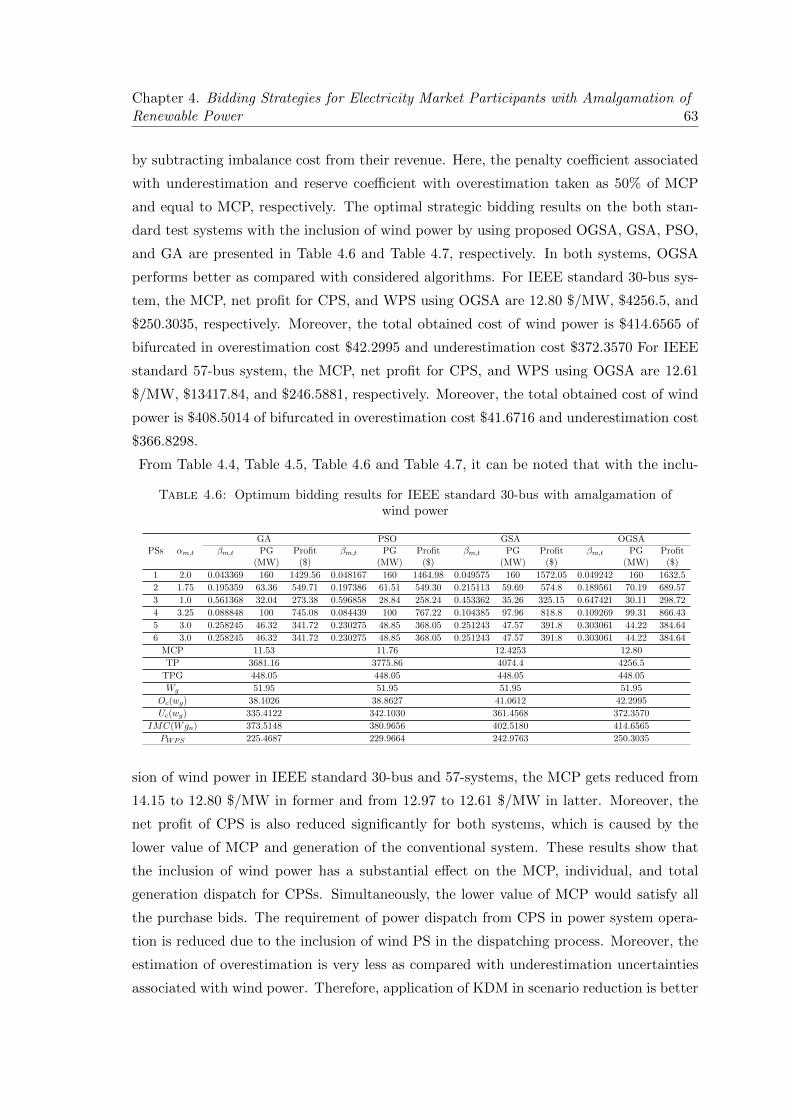
Chapter 4. Bidding Strategies for Electricity Market Participants with Amalgamation ofRenewable Power 63
by subtracting imbalance cost from their revenue. Here, the penalty coefficient associated
with underestimation and reserve coefficient with overestimation taken as 50% of MCP
and equal to MCP, respectively. The optimal strategic bidding results on the both stan-
dard test systems with the inclusion of wind power by using proposed OGSA, GSA, PSO,
and GA are presented in Table 4.6 and Table 4.7, respectively. In both systems, OGSA
performs better as compared with considered algorithms. For IEEE standard 30-bus sys-
tem, the MCP, net profit for CPS, and WPS using OGSA are 12.80 $/MW, $4256.5, and
$250.3035, respectively. Moreover, the total obtained cost of wind power is $414.6565 of
bifurcated in overestimation cost $42.2995 and underestimation cost $372.3570 For IEEE
standard 57-bus system, the MCP, net profit for CPS, and WPS using OGSA are 12.61
$/MW, $13417.84, and $246.5881, respectively. Moreover, the total obtained cost of wind
power is $408.5014 of bifurcated in overestimation cost $41.6716 and underestimation cost
$366.8298.
From Table 4.4, Table 4.5, Table 4.6 and Table 4.7, it can be noted that with the inclu-
Table 4.6: Optimum bidding results for IEEE standard 30-bus with amalgamation ofwind power
PSs αm,t
GA PSO GSA OGSAβm,t PG Profit βm,t PG Profit βm,t PG Profit βm,t PG Profit
(MW) ($) (MW) ($) (MW) ($) (MW) ($)
1 2.0 0.043369 160 1429.56 0.048167 160 1464.98 0.049575 160 1572.05 0.049242 160 1632.5
2 1.75 0.195359 63.36 549.71 0.197386 61.51 549.30 0.215113 59.69 574.8 0.189561 70.19 689.57
3 1.0 0.561368 32.04 273.38 0.596858 28.84 258.24 0.453362 35.26 325.15 0.647421 30.11 298.72
4 3.25 0.088848 100 745.08 0.084439 100 767.22 0.104385 97.96 818.8 0.109269 99.31 866.43
5 3.0 0.258245 46.32 341.72 0.230275 48.85 368.05 0.251243 47.57 391.8 0.303061 44.22 384.64
6 3.0 0.258245 46.32 341.72 0.230275 48.85 368.05 0.251243 47.57 391.8 0.303061 44.22 384.64
MCP 11.53 11.76 12.4253 12.80
TP 3681.16 3775.86 4074.4 4256.5
TPG 448.05 448.05 448.05 448.05
Wg 51.95 51.95 51.95 51.95
Oc(wg) 38.1026 38.8627 41.0612 42.2995
Uc(wg) 335.4122 342.1030 361.4568 372.3570
IMC(Wgn) 373.5148 380.9656 402.5180 414.6565
PWPS 225.4687 229.9664 242.9763 250.3035
sion of wind power in IEEE standard 30-bus and 57-systems, the MCP gets reduced from
14.15 to 12.80 $/MW in former and from 12.97 to 12.61 $/MW in latter. Moreover, the
net profit of CPS is also reduced significantly for both systems, which is caused by the
lower value of MCP and generation of the conventional system. These results show that
the inclusion of wind power has a substantial effect on the MCP, individual, and total
generation dispatch for CPSs. Simultaneously, the lower value of MCP would satisfy all
the purchase bids. The requirement of power dispatch from CPS in power system opera-
tion is reduced due to the inclusion of wind PS in the dispatching process. Moreover, the
estimation of overestimation is very less as compared with underestimation uncertainties
associated with wind power. Therefore, application of KDM in scenario reduction is better
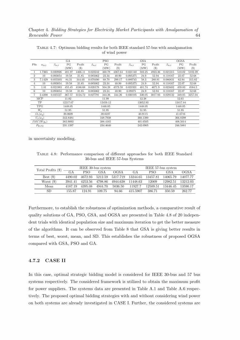
Chapter 4. Bidding Strategies for Electricity Market Participants with Amalgamation ofRenewable Power 64
Table 4.7: Optimum bidding results for both IEEE standard 57-bus with amalgamationof wind power
PSs αm,t
GA PSO GSA OGSAβm,t PG Profit βm,t PG Profit βm,t PG Profit βm,t PG Profit
(MW) ($) (MW) ($) (MW) ($) (MW) ($)
1 1.7365 0.020926 481.97 4466.11 0.022242 460.78 4367.64 0.021140 503.25 4923.36 0.021315 510.02 5102.39
2 10 0.093054 19.58 31.85 0.085062 23.34 40.90 0.095375 24.9 52.94 0.118167 22.07 52.68
3 7.1429 0.055503 84.31 344.03 0.070490 68.70 299.17 0.089745 58.3 280.91 0.086831 62.94 315.82
4 10 0.093054 19.58 31.85 0.085062 23.34 40.90 0.095375 24.9 52.94 0.118167 22.07 52.68
5 1.81 0.021983 455.45 4186.68 0.020178 504.28 4573.59 0.021931 481.74 4671.9 0.023482 459.83 4584.5
6 10 0.093054 19.58 31.85 0.085062 23.24 40.90 0.09375 24.9 52.94 0.118167 22.07 52.68
7 2.4390 0.025527 367.57 3124.72 0.027791 344.26 344.26 0.030105 330.05 3017.93 0.029132 349.05 3257.04
MCP 11.82 11.99 12.38 12.61
TP 12217.07 12459.12 13052.93 13417.84
TPG 1448.05 1448.05 1448.05 1448.05
Wg 51.95 51.95 51.95 51.95
Oc(wg) 39.0609 39.6227 40.9115 41.6716
Uc(wg) 343.8484 348.7938 360.1390 366.8298
IMC(Wgn) 382.9093 388.4165 401.0505 408.5014
PWPS 231.1397 234.4640 242.0905 246.5881
in uncertainty modeling.
Table 4.8: Performance comparison of different approaches for both IEEE Standard30-bus and IEEE 57-bus Systems
Total Profits ($)IEEE 30-bus system IEEE 57-bus system
GA PSO GSA OGSA GA PSO GSA OGSA
Best ($) 4490.02 4672.93 5212.59 5317.719 13244.65 13457.81 14065.79 14077.77
Worst ($) 3941.41 4253.56 4798.86 4944.638 11448.63 12009 12982.51 13212.03
Mean 4187.19 4395.08 4944.70 5036.50 11927.7 12509.51 13446.45 13590.17
SD 155.87 124.91 109.75 94.66 415.5907 386.71 350.59 262.77
Furthermore, to establish the robustness of optimization methods, a comparative result of
quality solutions of GA, PSO, GSA, and OGSA are presented in Table 4.8 of 20 indepen-
dent trials with identical population size and maximum iteration to get the better measure
of the algorithms. It can be observed from Table 8 that GSA is giving better results in
terms of best, worst, mean, and SD. This establishes the robustness of proposed OGSA
compared with GSA, PSO and GA.
4.7.2 CASE II
In this case, optimal strategic bidding model is considered for IEEE 30-bus and 57 bus
systems respectively. The considered framework is utilized to obtain the maximum profit
for power suppliers. The systems data are presented in Table A.1 and Table A.6 respec-
tively. The proposed optimal bidding strategies with and without considering wind power
on both systems are already investigated in CASE I. Further, the considered systems are

Chapter 4. Bidding Strategies for Electricity Market Participants with Amalgamation ofRenewable Power 65
modified to accommodate one solar power supplier to extent the influence of combined
wind and solar source. One solar and wind supplier of each 200 MW rated capacity is
assumed in this work. The suggested formulation is solved on a 3.20 GHz, i5 processor,
4GB RAM PC using the OGSA in MATLAB R2014a.
For the wind power estimation, compared to previous case I, in this case the planning
period is considered as 1300–1400 hrs from 1 august to 31 August 2005 of Barnstable city,
Massachusetts, USA [93]. The Air density and shear coefficient value are 1.242 kg/m3
and 0.35 respectively. The wind turbine VENSYS-100 and 2.5 MW capacity generator
is located at 100-meter hub height (VENSYS Wind Turbines) are used to generate wind
power. The wind speed data is fitted into a various probability distributions are shown in
Figure 4.3.
The Log Likelihood, Mean, and Variance values are calculated using various distributions
Figure 4.3: Curve fitting of the historical single hour (1300-1400 hrs) wind speed dataof Barnstable city, MA, USA for different distributions
and are presented in Table 4.9. It should be noted that the log-likelihood value of Weibull
distribution is better than others, indicating best fitting of the data in the distribution.
Shape and scale parameters values 3.34 and 7.93 m/s are calculated using (4.2) and (4.3)
respectively. Then, a thousand wind speed scenarios are generated and convert into power
scenarios using wind speed-power relationship. The each generated scenario assigned a
probability of normalization obtained using Weibull distribution to make their summation
equal to unity. The Weibull and normalize the density function of probabilities shown in
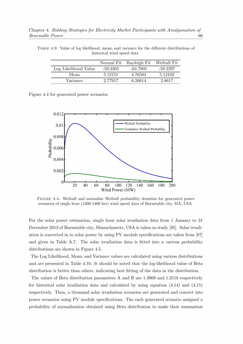
Chapter 4. Bidding Strategies for Electricity Market Participants with Amalgamation ofRenewable Power 66
Table 4.9: Value of log likelihood, mean, and variance for the different distributions ofhistorical wind speed data
Normal Fit Rayleigh Fit Weibull Fit
Log Likelihood Value -59.3305 -64.7905 -59.2297
Mean 5.12151 4.76584 5.12102
Variance 2.77917 6.20614 2.8617
Figure 4.4 for generated power scenarios.
Figure 4.4: Weibull and normalise Weibull probability densities for generated powerscenarios of single hour (1300-1400 hrs) wind speed data of Barnstable city, MA, USA
For the solar power estimation, single hour solar irradiation data from 1 January to 31
December 2013 of Barnstable city, Massachusetts, USA is taken as study [95]. Solar irradi-
ation is converted in to solar power by using PV module specifications are taken from [87]
and given in Table A.7. The solar irradiation data is fitted into a various probability
distributions are shown in Figure 4.5.
The Log Likelihood, Mean, and Variance values are calculated using various distributions
and are presented in Table 4.10. It should be noted that the log-likelihood value of Beta
distribution is better than others, indicating best fitting of the data in the distribution.
The values of Beta distribution parameters A and B are 1.3909 and 1.2518 respectively
for historical solar irradiation data and calculated by using equation (4.14) and (4.15)
respectively. Then, a thousand solar irradiation scenarios are generated and convert into
power scenarios using PV module specifications. The each generated scenario assigned a
probability of normalization obtained using Beta distribution to make their summation
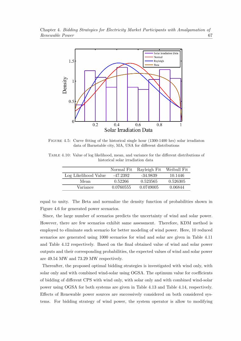
Chapter 4. Bidding Strategies for Electricity Market Participants with Amalgamation ofRenewable Power 67
Figure 4.5: Curve fitting of the historical single hour (1300-1400 hrs) solar irradiatondata of Barnstable city, MA, USA for different distributions
Table 4.10: Value of log likelihood, mean, and variance for the different distributions ofhistorical solar irradiation data
Normal Fit Rayleigh Fit Weibull Fit
Log Likelihood Value -47.2392 -34.9839 10.1446
Mean 0.52266 0.523565 0.526305
Variance 0.0760555 0.0749005 0.06844
equal to unity. The Beta and normalize the density function of probabilities shown in
Figure 4.6 for generated power scenarios.
Since, the large number of scenarios predicts the uncertainty of wind and solar power.
However, there are few scenarios exhibit same assessment. Therefore, KDM method is
employed to eliminate such scenario for better modeling of wind power. Here, 10 reduced
scenarios are generated using 1000 scenarios for wind and solar are given in Table 4.11
and Table 4.12 respectively. Based on the final obtained value of wind and solar power
outputs and their corresponding probabilities, the expected values of wind and solar power
are 49.54 MW and 73.29 MW respectively.
Thereafter, the proposed optimal bidding strategies is investigated with wind only, with
solar only and with combined wind-solar using OGSA. The optimum value for coefficients
of bidding of different CPS with wind only, with solar only and with combined wind-solar
power using OGSA for both systems are given in Table 4.13 and Table 4.14, respectively.
Effects of Renewable power sources are successively considered on both considered sys-
tems. For bidding strategy of wind power, the system operator is allow to modifying

Chapter 4. Bidding Strategies for Electricity Market Participants with Amalgamation ofRenewable Power 68
Figure 4.6: Beta and normalise Beta probability densities for generated power scenariosof single hour (1300-1400 hrs) wind speed data of Barnstable city, MA, USA
Table 4.11: Final KDM with wind power outputs and their probabilities for reducedten numbers of scenarios
Index 1 2 3 4 5 6 7 8 9 10 Wa (MW) Probability Min (KD)
1 0 27.85 51.7 76.35 92.08 108.9 127.1 141.2 164.8 179.5 14.39 0.234229 27.85
2 27.85 0 23.85 48.5 64.23 81.06 99.26 113.4 136.9 151.6 42.24 0.443626 23.85
3 51.70 23.85 0 24.65 40.37 57.21 75.41 89.52 113.1 127.8 66.09 0.17126 23.85
4 76.35 48.5 24.65 0 15.73 32.56 50.76 64.87 88.43 103.1 90.74 0.080668 15.73
5 92.08 64.23 40.37 15.73 0 16.84 35.04 49.15 72.71 87.40 106.5 0.025689 15.73
6 108.9 81.06 57.21 32.56 16.84 0 18.20 32.31 55.87 70.56 123.3 0.025047 16.84
7 127.1 99.26 75.41 50.76 35.04 18.20 0 14.11 37.67 52.36 141.5 0.011009 14.11
8 141.2 113.4 89.52 64.87 49.15 32.31 14.11 0 23.56 38.25 155.6 0.005085 14.11
9 164.8 136.9 113.1 88.43 72.71 55.87 37.67 23.56 0 14.69 179.2 0.002536 14.69
10 179.5 151.6 127.8 103.1 87.39 70.56 52.36 38.25 14.69 0 193.9 0.000852 14.69
Table 4.12: Final KDM with solar power outputs and their probabilities for reducedten numbers of scenarios
Index 1 2 3 4 5 6 7 8 9 10 Wa (MW) Probability Min (KD)
1 0 11.42 34.23 46.35 62.47 80.47 98.7 114.8 131.1 150.2 16 0.022218 11.42
2 11.42 0 22.81 34.93 51.05 69.31 87.28 103.4 119.7 138.8 27.42 0.075345 11.42
3 34.23 22.81 0 12.12 28.24 46.5 64.47 80.60 96.85 116 50.23 0.268311 12.12
4 46.35 34.93 12.12 0 16.12 34.38 52.35 68.49 84.73 103.9 62.35 0.163971 12.12
5 62.47 51.05 28.24 16.12 0 18.27 36.23 52.37 68.62 87.76 78.47 0.277874 16.12
6 80.73 69.31 46.50 34.38 18.27 0 17.97 34.1 50.35 69.49 96.74 0.09117 17.97
7 98.7 87.28 64.47 52.35 36.23 17.97 0 16.13 32.38 51.53 114.7 0.046975 16.13
8 114.8 103.4 80.6 68.49 52.37 34.10 16.13 0 16.25 35.39 130.8 0.042748 16.13
9 131.1 119.7 96.85 84.73 68.62 50.35 32.38 16.25 0 19.14 147.1 0.00999 16.25
10 150.2 138.8 116 103.9 87.76 69.49 51.53 35.39 19.14 0 166.2 0.001399 19.14

Chapter 4. Bidding Strategies for Electricity Market Participants with Amalgamation ofRenewable Power 69
the existing demand, which means actual demand excluding wind power generation, and
then updates the bidding coefficients in accordance with the changing demand [50]. Based
on this approach wind and solar power are considered to determine the new MCP. First
the wind power generator is considered and new value of MCP is calculated by updating
the bidding coefficients at modified demand. Similarly, MCP with the inclusion of solar
power and finally, the aggregate benefits of wind and solar generator are considered. In
this analysis, the consideration of operating cost for both the renewable sources has not
been taken into account. However, due to the associated intermittency of these renewable
sources it is acceptable to consider their imbalance cost. This cost is determined in terms
of overestimation and underestimation of generation from both solar and wind. And the
effect of this cost is reflected on total profit obtained by renewable suppliers in terms of
revenue minus the imbalance cost. Also, the penalty coefficient and reserve coefficient
linked with underestimation and overestimation separately are considered as 50% of MCP
and equivalent to MCP respectively. The results of proposed bidding strategy on con-
sidered systems with only wind, with only solar and with combined wind-solar by using
OGSA are presented in Table 4.13 and Table 4.14, respectively.
It is observed that from the case I Table 4.4, the market is cleared at MCP value of 14.15
Table 4.13: Optimum bidding results for IEEE 30-bus with amalgamation of wind andsolar power
PSs αm,t
with wind only with solar only with both wind and solarβm,t PG Profit βm,t PG Profit βm,t PG Profit
(MW) ($) (MW) ($) (MW) ($)
1 2.0 0.049984 160 1661.96 0.049886 160 1570.03 0.050156 160 432.87
2 1.75 0.223528 64.70 653.79 0.208066 60.99 585.25 0.229582 48.81 436.93
3 1.0 0.680919 32.03 319.85 0.747376 25.02 246.39 0.66874 21.89 201.09
4 3.25 0099466 100 890.32 0.108838 93.93 787.09 0.109776 81.76 623.31
5 3.0 0.307913 46.86 413.13 0.279827 43.38 361.31 0.325901 32.35 250.64
6 3.0 0.307913 46.86 413.13 0.279827 43.38 361.31 0.325901 32.35 250.64
MCP ($/MW) 12.99 12.41 11.56
TCPS ($) 4352.19 3911.38 3195.48
TPG-CPS (MW) 450.46 426.71 377.17
RPG (MW) 49.5406 73.2897 49.5406 (W), 73.2897 (S)
OCRs ($) 46.7718 119.1724 41.6230(W), 111.0099(S)
UCRs ($) 368.7903 257.9840 328.1921(W), 240.3139(S)
IMCRs ($) 415.5621 377.1564 369.8151(W), 351.3238(S)
PRs ($) 227.9703 532.3688 202.8742(W), 495.9051(S)
$/MW, total generation of CPS is 500 MW and net profit is $5317.72 with IEEE stan-
dard 30 bus system without considering wind and solar power. But if only wind power is
included with CPS then MCP is reduced to 12.99 $/MW and total generation of CPS is re-
duced to 450.46 MW. In addition, CPS’ net profit is also significantly reduced by $4352.19,
which is caused by the lower value of MCP and conventional system generation. The wind
power net profit, overestimation and underestimation costs are $227.9703, $46.7718 and

Chapter 4. Bidding Strategies for Electricity Market Participants with Amalgamation ofRenewable Power 70
$368.7903 respectively. In the second case i.e. only solar power with CPS, the net profit
value, overestimation and underestimation costs are 532.3688, $119.1724, and $257.9840
respectively. For this case, the MCP value is 12.41 $/MW with total generation of CPS
426.71 MW which is lower than conventional and wind due to significant power generation
from the solar. Finally, when both the wind and solar are considered with CPS, MCP is
11.56 $/MW, which is lowest among all previous considered cases.
Similarly, From Table 4.5, it is observed that the market is cleared at MCP value of 12.97
Table 4.14: Optimum bidding results for IEEE 57-bus with amalgamation of wind andsolar power
PSs αm,t
with wind only with solar only with both wind and solarβm,t PG Profit βm,t PG Profit βm,t PG Profit
(MW) ($) (MW) ($) (MW) ($)
1 1.7365 0.021880 501.65 5078.29 0.022239 485.76 4846.56 0.022531 466.59 4535.04
2 10 0.123756 21.92 54.65 0.076760 33.08 73.07 0.094126 23.9 48.04
3 7.1429 0.071514 77.88 390.7 0.088860 60.73 301.56 0.076142 67.06 310.52
4 10 0.123756 21.92 54.65 0.076760 33.08 73.07 0.094126 23.9 48.04
5 1.81 0.023322 467.47 4703.2 0.023240 461.68 4569.9 0.024014 434.71 4197.96
6 10 0.123756 21.92 54.65 0.076760 33.08 73.07 0.094126 23.9 48.04
7 2.4390 0.030421 337.71 3195.7 0.031635 319.29 2980.3 0.029101 337.11 3034.43
MCP ($/MW) 12.71 12.54 12.25
TCPS ($) 13531.86 12917.50 12222.07
TPG-CPS (MW) 1450.46 1426.7103 1377.1697
RPG (MW) 49.5406 73.2897 49.5406 (W), 73.2897 (S)
OCRs ($) 45.7637 120.4208 44.1074(W), 117.6360(S)
UCRs ($) 360.8410 260.6865 347.7815(W), 254.6578(S)
IMCRs ($) 406.6047 381.1073 391.8888(W), 372.2938(S)
PRs ($) 223.0564 537.9455 214.9835(W), 525.5050(S)
$/MW, total generation of CPS is 1500 MW and net profit is $14077.77. But if only wind
power is included with CPS then MCP is reduced to 12.71 $/MW and total generation of
CPS is reduced to 1450.46 MW. In addition, CPS net profit is also significantly reduced by
$1426.7103, which is caused by the lower value of MCP and conventional system genera-
tion. The wind power net profit, overestimation and underestimation costs are $223.0564,
$45.7637 and $360.8410 respectively. In the second case i.e. only solar power with CPS,
the net profit value, overestimation and underestimation costs are $537.9455, $120.4208,
and $260.6865 respectively. For this case, the MCP value is 12.54 $/MW with total gener-
ation of CPS 1426.7103 MW which is lower than conventional and wind due to significant
power generation from the solar. Finally, when both the wind and solar are considered
with CPS, MCP is 12.25 $/MW, which is lowest among all previous considered cases.
From Table 4.13 and Table 4.14, it can be observed that all the purchase bids would satisfy
by the lower MCP value. Due to the presence of solar and wind suppliers in the process
of dispatch, there will be fewer CPS requirements in power system operation. Further,
the overestimation estimate is very small compared to the underestimation of solar and

Chapter 4. Bidding Strategies for Electricity Market Participants with Amalgamation ofRenewable Power 71
wind power uncertainties. Therefore, applying KDM in reduction of scenarios is better
in modeling uncertainty. This will encourage to the solar and wind power suppliers for
bidding the extra power into the real-time market if the underestimation is positive.
4.7.3 CASE III
In this case, the double sided optimal strategic bidding model is analytically tested on
IEEE 30-bus system, and the system data for suppliers and large buyers is presented in
Table A.5. The system consist of six conventional power suppliers (CPS) and two large
consumers. Also, the value of constant load demand is 300 MW with load price elasticity
(k=5) at the time of bidding for IEEE 30-bus system. The proposed framework is utilized
to obtain the maximum profit for power suppliers and large buyers. The proposed optimal
bidding strategies without considering wind and solar power on system is already investi-
gated in Chapter 3, CASE III. Further, the considered model is modified to accommodate
one solar and one wind power supplier to the extent the influence of solar and wind source.
In this work, one supplier of wind and solar of each rated capacity of 200 MW are con-
sidered. The proposed model has beeen framed as a multi-objective optimization problem
and solved by using TOPSIS amalgamation with OGSA (TOGSA) in MATLAB R2014a
on a 3.20 GHz, i5 processor, 4GB RAM PC.
For the wind power estimation, single hour wind speed data from 1 August to 31 August
2005 of Barnstable city, Massachusetts, USA [93]. The air density and shear coefficient
value are 1.242 kg/m3 and 0.35 respectively. The wind turbine VENSYS-100 and 2.5 MW
capacity generator located at 100-meter hub height are used to generate wind power. The
wind speed data is fitted into various probability distributions are shown in Figure 4.7.
The values of log likelihood, mean and variance are calculated using various distributions
and are presented in Table 4.15. It should be noted that the log-likelihood value of Weibull
distribution is better than others, indicating best fitting of the data in the distribution.
The values of shape and scale parameters calculated using (4.2) and (4.3) are 3.3094
Table 4.15: Value of log likelihood, mean, and variance for the different distributions ofhistorical wind speed data
Normal Fit Rayleigh Fit Weibull Fit
Log Likelihood Value -60.742 -65.6732 -60.4794
Mean 5.20054 4.85338 5.20428
Variance 3.04414 6.43624 2.99978
and 8.0654 m/s respectively. Then, a thousand wind speed scenarios are generated and
converted into power scenarios using wind speed-power relationship. A normalization
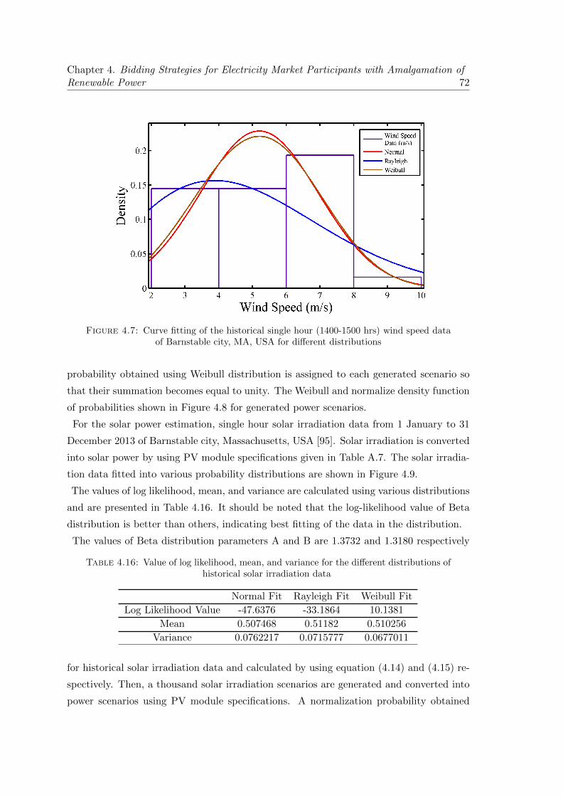
Chapter 4. Bidding Strategies for Electricity Market Participants with Amalgamation ofRenewable Power 72
Figure 4.7: Curve fitting of the historical single hour (1400-1500 hrs) wind speed dataof Barnstable city, MA, USA for different distributions
probability obtained using Weibull distribution is assigned to each generated scenario so
that their summation becomes equal to unity. The Weibull and normalize density function
of probabilities shown in Figure 4.8 for generated power scenarios.
For the solar power estimation, single hour solar irradiation data from 1 January to 31
December 2013 of Barnstable city, Massachusetts, USA [95]. Solar irradiation is converted
into solar power by using PV module specifications given in Table A.7. The solar irradia-
tion data fitted into various probability distributions are shown in Figure 4.9.
The values of log likelihood, mean, and variance are calculated using various distributions
and are presented in Table 4.16. It should be noted that the log-likelihood value of Beta
distribution is better than others, indicating best fitting of the data in the distribution.
The values of Beta distribution parameters A and B are 1.3732 and 1.3180 respectively
Table 4.16: Value of log likelihood, mean, and variance for the different distributions ofhistorical solar irradiation data
Normal Fit Rayleigh Fit Weibull Fit
Log Likelihood Value -47.6376 -33.1864 10.1381
Mean 0.507468 0.51182 0.510256
Variance 0.0762217 0.0715777 0.0677011
for historical solar irradiation data and calculated by using equation (4.14) and (4.15) re-
spectively. Then, a thousand solar irradiation scenarios are generated and converted into
power scenarios using PV module specifications. A normalization probability obtained

Chapter 4. Bidding Strategies for Electricity Market Participants with Amalgamation ofRenewable Power 73
Figure 4.8: Weibull and normalise Weibull probability densities for generated powerscenarios of single hour (1400-1500 hrs) wind speed data of Barnstable city, MA, USA
using Beta distribution is assigned to each generated scenario so that their summation
becomes equal to unity. The Beta and Normalize density function of probabilities shown
in Figure 4.10 for generated power scenarios.
Since, the large number of scenarios predicts the uncertainty of wind and solar power.
However, there are few scenarios exhibiting the same assessment. Therefore, KDM method
is employed to eliminate such scenario for better modeling of wind power. Here, 10 re-
duced scenarios generated using 1000 scenarios for wind and solar are given in Table 4.17
and Table 4.18, respectively. Based on the final obtained value of wind and solar power
outputs and their corresponding probabilities, the expected values of wind and solar power
are 50.31 MW and 70.76 MW respectively.
The optimal double sided strategic bidding model is framed as a multi objective opti-
mization problem and tested on considered system in Chapter 3, case III. Results for the
considered system show that the proposed technique TOGSA is more suitable as compared
to GSA and MC. Therefore, in this case modified test system is considered with wind pow-
er only, with solar only and with combined wind-solar and solved by using TOGSA.
Renewable based power sources in the modified system are successively considered to mea-
sure the effect of renewable. System operators are allowed to modify existing demand that
means actual demand excluding generation from wind power for strategic bidding of wind
power on the emerging power market, system operator is permitted to modify the existing

Chapter 4. Bidding Strategies for Electricity Market Participants with Amalgamation ofRenewable Power 74
Figure 4.9: Curve fitting of the historical single hour (1400-1500 hrs) solar irradiationdata of Barnstable city, MA, USA for different distributions
Table 4.17: Final KDM with wind power outputs and their probabilities for reducedten numbers of scenarios
Index 1 2 3 4 5 6 7 8 9 10 Wa (MW) Probability Min (KD)
1 0 17.39 45.38 63.97 79.87 97.11 121.5 136.3 150.2 165.5 29.22 0.546236 17.39
2 17.39 0 27.99 46.58 62.48 79.72 104.1 118.9 132.8 148.1 46.62 0.181994 17.39
3 45.38 27.99 0 18.59 34.49 51.73 76.12 90.90 104.8 120.1 74.61 0.105963 18.59
4 63.97 46.58 18.59 0 15.9 33.14 57.53 72.31 86.24 101.5 93.2 0.087006 15.9
5 79.87 62.48 34.49 15.9 0 17.24 41.63 56.41 70.34 85.62 109.1 0.037677 15.9
6 97.11 79.72 51.73 33.14 17.24 0 24.39 39.17 53.1 68.38 126.3 0.026649 17.24
7 121.5 104.1 76.12 57.53 41.63 24.39 0 14.78 28.71 43.99 150.7 0.004927 14.78
8 136.3 118.9 90.9 72.31 56.41 39.17 14.78 0 13.93 29.21 165.5 0.006487 13.93
9 150.2 132.8 104.8 86.24 70.34 53.1 28.71 13.93 0 15.28 179.4 0.002440 13.93
10 165.5 148.1 120.1 101.5 85.62 68.38 43.99 29.21 15.28 0 194.7 0.000622 15.28
demand and then updating the coefficients of bidding in agreement with the modifying
demand. Based on this approach wind and solar power are considered to determine the
new MCP. First the wind power generator is considered and new value of MCP is calcu-
lated by updating the bidding coefficients at modified demand. Similarly, MCP with the
inclusion of solar power and finally, the aggregate benefits of wind and solar generator are
considered. In this analysis, the consideration of operating cost for both the renewable
sources has not been taken into account. However, due to the associated intermittency of
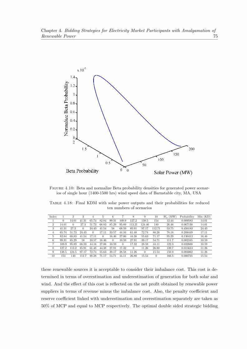
Chapter 4. Bidding Strategies for Electricity Market Participants with Amalgamation ofRenewable Power 75
Figure 4.10: Beta and normalize Beta probability densities for generated power scenar-ios of single hour (1400-1500 hrs) wind speed data of Barnstable city, MA, USA
Table 4.18: Final KDM with solar power outputs and their probabilities for reducedten numbers of scenarios
Index 1 2 3 4 5 6 7 8 9 10 Wa (MW) Probability Min (KD)
1 0 14.01 41.31 65.74 82.84 99.31 109.9 127.2 138.5 154 12.44 0.009583 14.01
2 14.01 0 27.3 51.73 68.83 85.29 95.89 113.21 124.46 140 26.46 0.067130 14.01
3 41.31 27.3 0 24.43 41.54 58 68.59 85.91 97.17 112.71 53.75 0.450183 24.43
4 65.74 51.73 24.43 0 17.11 33.57 44.16 61.48 72.74 88.28 78.18 0.208449 17.11
5 82.84 68.83 41.54 17.11 0 16.46 27.06 44.38 55.63 71.17 95.29 0.130413 16.46
6 99.31 85.29 58 33.57 16.46 0 10.59 27.91 39.17 54.71 111.7 0.082165 10.59
7 109.9 95.89 68.59 44.16 27.06 10.59 0 17.32 28.58 44.11 122.3 0.032668 10.59
8 127.2 113.2 85.91 61.48 44.38 27.91 17.32 0 11.26 26.80 139.7 0.015613 11.26
9 138.5 124.5 97.17 72.74 55.63 39.17 28.58 11.26 0 15.54 150.9 0.003062 11.26
10 154 140 112.7 88.28 71.17 54.71 44.11 26.80 15.54 0 166.5 0.000735 15.54
these renewable sources it is acceptable to consider their imbalance cost. This cost is de-
termined in terms of overestimation and underestimation of generation for both solar and
wind. And the effect of this cost is reflected on the net profit obtained by renewable power
suppliers in terms of revenue minus the imbalance cost. Also, the penalty coefficient and
reserve coefficient linked with underestimation and overestimation separately are taken as
50% of MCP and equal to MCP respectively. The optimal double sided strategic bidding

Chapter 4. Bidding Strategies for Electricity Market Participants with Amalgamation ofRenewable Power 76
results on modified test system with wind power only, with solar power only and with
combined wind-solar power by using TOGSA are given in Table 4.19.
Table 4.19: Optimum bidding results for IEEE 30-bus with amalgamation of wind andsolar power
PSs αm,t
with wind only with solar only with both wind and solarβm,t PG Profit βm,t PG Profit βm,t PG Profit
(MW) ($) (MW) ($) (MW) ($)
1 6.0 0.074476 145.76 1260.40 0.032677 160 1323.61 0.024928 160 1278.21
2 5.25 0.130126 92.46 571.64 0.154422 97.53 556.14 0.428093 55.63 423.80
3 3.0 0.949644 27.64 262.20 0.52532 52.33 307.55 0.837573 45.63 297.26
4 9.75 0.039809 120 419.81 0.202882 58.61 283.58 0.094028 89.85 338.18
5 9.0 0.207086 42.83 174.51 0.488099 47.44 166.73 0.899081 45.63 153.61
6 9.0 0.207086 42.83 174.51 0.488099 47.44 166.73 0.899081 45.63 153.61
Total 471.51 2863.07 463.36 2804.34 442.37 2644.68
LBs φn,t ϕn,t CD Benefit ϕn,t CD Benefit ϕn,t CD Benefit(MW) ($) (MW) ($) (MW) ($)
1 30 0.073966 185.40 1167.50 0.081677 170.52 1211.82 0.073867 192.39 1253.54
2 25 0.073931 117.86 610.20 0.062013 143.96 663.46 0.041960 150 706.68
Total 303.25 1777.7 314.48 1875.28 342.39 1960.22
MCP ($/MW) 16.29 16.07 15.79
Q(MCP) (MW) 218.57 219.64 221.06
TPT(MW) 521.57 534.12 563.45
RPG (MW) 50.31 70.76 50.31(W), 70.76(S)
OCRs ($) 58.6422 153.55 56.84(W), 150.88(S)
UCRs ($) 468.20 328.20 453.83(W), 322.48(S)
IMCRs ($) 526.84 481.75 510.67(W), 473.36(S)
PRs ($) 292.71 655.36 283.72(W), 643.94(S)
From Table 3.8, it is observed that from the Chapter 3 in case III, the market is cleared
at MCP value of 16.50 $/MW, total generation of CPS is 520.2 MW, total demand of
large consumers is 302.7 MW, total power traded is 520.2 MW, and net profit for CPS
and large consumers are $3140.4 and $1729.1 respectively. From Table 4.19, it is observed
that when only wind power is included with CPS then MCP is reduced to 16.29 $/MW,
total generation of CPS is reduced to 471.51 MW, total demand of large consumers and
total traded power are increased to 303.25 MW and 521.57 MW respectively, and the
net profit of CPS is reduced to $2863.07 which is caused by the lower value of MCP and
generation of CPS. Moreover, the net profit of large consumers is increased significantly,
which is caused by the lower value of MCP and higher demand of large consumers. The
wind power net profit, overestimation and underestimation costs are $292.71, $58.64 and
$468.20 respectively. In the second case i.e. only solar power with CPS, the net profit value,
overestimation and underestimation costs are $655.36, $153.55, and $328.20 respectively.
For this case, the MCP value is 16.07 $/MW, total generation of CPS 463.36 MW which
is lower than conventional and wind due to significant power generation from the solar,
total demand of large consumers and total traded power are increased to 314.48 MW and
534.12 respectively. Finally, when both the wind and solar are considered with CPS, MCP

Chapter 4. Bidding Strategies for Electricity Market Participants with Amalgamation ofRenewable Power 77
is 15.79 $/MW, which is lowest among all previous considered cases. From the obtained
results, it can be observed that, due to the lower MCP value large number of customers
gets attracted to buy more power which results in increased total power trade and finally
satisfying all the purchase bids. Also, due to the integration of solar and wind power
suppliers in the system the requirement of supply from CPS is highly reduced. Further,
with the involvement of KDM, overestimation of uncertainty is very less as compared to
the underestimation in both the solar and wind power generation. This will encourage the
solar and wind power suppliers for bidding the extra power into the real-time market if
the underestimation is positive.
4.8 Conclusions
In this section, single sided and double sided bidding strategy with inclusion of renewable
energy sources have been evaluated to maximize profit of different market entities. A
heuristic technique, OGSA is used to solve single sided bidding strategy and TOGSA is
used to solve double sided bidding strategy. Wind speed and solar irradiation uncertainties
are handled respectively by Weibull and Beta distribution of probability, and transformed
into wind and solar power. Further, KDM method is used to reduce the samples of
wind and solar power. In addition, the renewable energy variability is measured in terms
of overestimation and underestimation. Furthermore, the uncertainty of the behaviour of
rival is minimized using the function of Normal distribution of probability. It is found that
from the obtained results, OGSA and TOGSA approaches are effective and promising to
obtain the most compromising solutions. Amalgamations of wind and solar power also
affects the bid as it reduces the CPS generation and provides less MCP value that would
deliver sufficient electricity from accepted sales bids to meet all accepted purchase bids and
increase the total traded power. Further, with the involvement of KDM, overestimation
of uncertainty is very less as compared to the underestimation in both the solar and wind
power generation. This will encourage the solar and wind power suppliers for bidding the
extra power into the real-time market if the underestimation is positive. Results for the
IEEE standard 30-bus and modified six supplier with two large buyers systems shows that
the proposed techniques in this chapter are more suitable to obtain the most compromising
solution for single and multi-objective strategic bidding problems of market participants.
In the next Chapter, the optimal coordinated bidding strategy between energy and reserve
markets for profit maximization of power suppliers has been examined using proposed

Chapter 4. Bidding Strategies for Electricity Market Participants with Amalgamation ofRenewable Power 78
OGSA in single side trading mechanism. And its performance has been evaluated and
compared with the available literature.

Chapter 5
Coordinating Bidding Strategy
between Energy and Reserve
Markets
5.1 Introduction
Deregulation process includes un-bundling of electric power generation from the trans-
mission system, which increases the requirements of ancillary services [96]. The ancillary
services are separated into various services such as spinning and non spinning reserves,
replacement reserves, Automatic Generation Control (AGC), black start, and voltage sup-
port. The ISO can procure the first four services by means of a daily competitive auction,
whereas the last two services are more suitable for long-term purchases. The primary
function of ancillary services are providing backup to power transmission network from
the power supplier to the buyer. These services are essential to confirm that the market
operators are capable of meeting their responsibilities [97]. Although, the objective of
specific ancillary service spinning reserve is to maintain a balance between power supply
and demand. Spinning reserve is an online generator’s ability to increase and decrease its
output in a short time. The main requirement of the spinning reserve is to maintain relia-
bility of the system [5]. In this chapter, GENCOs are assumed to participate in the energy
markets as well as in the reserve markets for ancillary services (only spinning reserves). In
this context, OGSA is employed to pick optimal bidding strategy for GENCO’s between
the sets of discrete bids.
79

Chapter 5. Coordinating Bidding Strategy between Energy and Reserve Markets 80
5.2 Market Clearing Mechanism in Energy and Spinning
Reserve Markets
In some market structures of electric power such as CAISO wholesale market, the in-
dependent system operator (ISO) and the power exchange (PX) are separate bodies, in
which, the PX manages the market of energy, and the ISO manages the market of spinning
reserve [5]. In this type of market structures, market participants may elect themself or
may select ISO on their behalf for buying required spinning reserve that is assisting in
maintaining their energy requirements. Based on the forecasted conditions of the system
and submitted plans from the scheduling coordinators (SCs) and PX , ISO first decides
the necessities for an extra spinning reserve of each case beyond those already provided by
the PX and the SCs as self-provision [98]. After this, ISO chooses and expenses the most
low-budget services from submitted bids of spinning reserve. For this reason, besides bid-
ding within the energy market, every power provider may have an enthusiasm for building
up a strategic bidding in the market of reserve too, with the goal of maximizing its total
profit. Hence, to attain the objective of total profit maximization, every power provider
appearances a decision-making issue on how to construct optimally coordinated bidding
strategy in electricity and spinning reserve markets.
5.2.1 Modeling of the PX
The main purpose of the PX is to manage the day-ahead energy market. After receiving
a bid from the power suppliers using the transparent dispatch procedures, PX sets the
generation output of active power that meets the total demand of the system. It is assumed
that each power supplier is required to submit a non-decreasing linear energy supply bid
function to the PX. Then PX determines a set of all suppliers generation outputs by
solving the following problem if only load flow (5.1) and output limit (5.2) constraints are
considered.
αm + βmPem = Re (5.1)
CPS∑m=1
P em = De (5.2)
P emin,m ≤ P em ≤ P emax,m (5.3)
Chapter 5. Coordinating Bidding Strategy between Energy and Reserve Markets 81
The solution of (5.1) and (5.2) are taken wihout considering (5.3). Hence, the solution of
(5.1) and (5.2) can be written as:
Re =
De +CPS∑m=1
αmβm
CPS∑m=1
1βm
(5.4)
P em =Re − αmβm
(5.5)
5.2.2 Modeling of the ISO
ISO managed spinning reserve in the ancillary services market. After receiving a bid of
spinning reserve from the power suppliers using the transparent dispatch procedures, ISO
sets the dispatch of spinning reserve of all suppliers such that it meets the total capacity of
required spinning reserve of the system. It is assumed that each power supplier is required
to submit a non-decreasing linear spinning reserve supply bid function to the ISO. ISO
ensures that (5.6) to (5.8) must satisfy the dispatch of the spinning reserve when the
security constraints (5.7) and reliability constraints (5.8) are considered.
ψm + ξmPsrm = Rsr (5.6)
CPS∑m=1
P srm = Dsr (5.7)
P srmin,m ≤ P srm ≤ P srmin,m (5.8)
The solution of equation (5.6) and (5.7) are presented, when (5.8) is ignored,
Rsr =
Dsr +CPS∑m=1
ψmξm
CPS∑m=1
1ξm
(5.9)
P srm =Rsr − ψm
ξm(5.10)

Chapter 5. Coordinating Bidding Strategy between Energy and Reserve Markets 82
5.3 Problem Formulation of Coordinating Bidding Strategy
between Energy And Reserve Markets for Profit Maxi-
mization of the Power Suppliers
Optimally coordinating bidding problem in energy and spinning reserve market for mth
power supplier profit maximization can be described as
Maximize
F (αm, βm, ψm, ξm) = Re × P em +Rsr × P srm − Cm(P em + Pnm) (5.11)
Subject to: Equation (5.1)-(5.3), (5.6)-(5.8) and
P emin,m ≤ P em ≤ P emin,m − P srm (5.12)
Where Cm(P em + Pnm) is the combined production cost of energy and reserve that is
Cm(P em + Pnm) = am(P em + Pnm) + bm(P em + Pnm)2 (5.13)
Generally, at the time of operation, actual amount of the spinning reserve is less than the
contracted amount utilized by the ISO. It is supposed that the capacity taken from the
individual power supplier will be proportional to the contracted capacity [99]. Further,
it has been assumed that a supplier is paid the price at MCP according to (5.9) for
maintaining contracted spinning reserves of (5.10) irrespective of its utilization as defined
in (5.11). Therefore, each supplier is required to determine the amount of consumed
spinning reserve considering all costs involved in its spinning reserve bid. Hence, the part
of spinning reserve consumed from its actual amount contracted with ISO is expressed as
Pnm = P srm ×(dms /Dsr
)= P srm ×Km (5.14)
As the amount of spinning reserve consumed is unknown in advance, ISO repeatedly con-
veys its requirement to power producers in real-time. This information help the producers
to approximate their spinning reserve capacity on the basis of prior knowledge and tenden-
cy to take risks. The possibility of selection of a producer’s bid is reduced if it overestimates
this capacity and offers a costly bid. The bidding coefficients of energy and reserve fol-
lows a normal joint PDF. Normal joint PDF of energy bidding coefficients (αm, βm) are
explained in chapter 3. Similarly, normal joint PDF [64] of reserve bidding coefficients
Chapter 5. Coordinating Bidding Strategy between Energy and Reserve Markets 83
(ψm, ξm) are
(ψm, ξm)j ∼ N
{[µ
(ψ)m
µ(ψ)m
],
(σ(ψ)m )
2γmσ
(ψ)m σ
(ξ)m
γmσ(ψ)m σ
(ξ)m (σ
(ξ)m )
2
(5.15)
5.4 Solution Procedure of OGSA Applied to Coordinated
Bidding Strategy Problem between Energy and Reserve
Market
1. Set input data of considered test system for power suppliers bidding strategy in
energy and reserve market. Also, set the parameters of the proposed OGSA.
2. Set population size (N) and randomly generate initial population λ for bidding co-
efficient βm,t of power suppliers in the decided search space of the problem.
3. Determine the market clearing price in energy market as (5.4) and in reserve market
as (5.9). Also, determine the dispatch of each generator in energy market as (5.5)
and in reserve market as (5.10) respectively.
4. Set power generation limits as (5.3) and reserve limits as (5.8) and balance the system
load in both markets.
5. Determine actual utilized reserve quantity as (5.14) than calculate profit of each
power supplier as (5.11).
6. Generate opposite population (Oλ) to the initial generated population (λ) in search
space. Then determine the market clearing price in energy market as (5.4) and in
reserve market as (5.9). Also, determine the dispatch of each generator in energy
market as (5.5) and in reserve market as (5.10) respectively.
7. Set power generation limits as (5.3) and reserve limits as (5.8) and balance the system
load in both markets.
8. Evaluate the fitness function for all random (λ) and opposite (Oλ) population.
9. Select N fittest agents from current (λ) and opposite population (Oλ) as current
population (λ).
10. Determine the mass of every agent as (2.4) and gravitational constant as (2.6) re-
spectively.

Chapter 5. Coordinating Bidding Strategy between Energy and Reserve Markets 84
11. Calculate all agents’ acceleration as (2.5).
12. Update the respective velocity and position of the agent as (2.7).
13. If the maximum number of iterations are not exceeded, go to Step 3, otherwise the
procedure will be stopped and the optimum bidding strategy printed.
5.5 Result and Discussion
In this section, optimal coordinated bidding strategy between energy and reserve markets
is considered for six generating units system. The considered framework is utilized to
obtain the maximum profit for power suppliers. The respective supplier’s output limits in
the spinning reserve market, energy market, and supplier’s fuel cost coefficients are given
in Table A.8 and taken from [65]. Also, the considered value of De and Dsr are 1000
MW and 100 MW respectively. The solution obtained by using OGSA is compared with
GSA and RGA [65] to demonstrate the capability of OGSA. The tuning parameters of the
OGSA are given in Table A.2. The simulations are carried out using MATLAB R2014a
software on 3.20 GHz, i5 processor, 4GB RAM PC.
For instance, the essential methodology of constructing the strategic bidding for the 6th
supplier is explained here. The overall output limit of the 6th supplier is 250 MW, and
this is the sum of its output limits in both markets. Estimated output limit of spinning
reserve for 6th supplier in scenario first and second is to be really used as 0.1 ×Dsr and
0.2×Dsr respectively. Subsequently K6 = 0.1 for scenario first and K6 = 0.2 for scenario
second has been obtained.
From the perspective of the 6th power supplier in the energy market, every one of the
five opponent power supplier is supposed to have an expected joint normal distribution
for the two coefficients of bidding, αm and βm, (m = 1, 2, . . . , 5). Similarly, from the
perspective of the 6th power supplier in the spinning reserve market, every one of the five
opponent power supplier is supposed to have an expected joint normal distribution for the
two coefficients of bidding, ψm and ξm, (m = 1, 2, . . . , 5).
The approximation of bidding coefficient’s in a joint normal distribution for the five oppo-
nents in energy and spinning reserve market are given in Table 5.1 and taken from [65] .
Therefore in this work, supplier fix the values of α6 = a6 and ψ6 = 0.5× b6, and employs
the OGSA to determine optimal values of β6 and ξ6 for developing its strategic bidding.
The optimal values of β6 and ξ6 are searched in the interval between [b6, 20b6] and [0, 10b6]

Chapter 5. Coordinating Bidding Strategy between Energy and Reserve Markets 85
Table 5.1: Estimation of parameters for the five opponents
Estimation of five opponents suppliers in energy market Estimation of five opponents suppliers in reserve market
µ(α)m µ
(β)m σ
(α)m σ
(β)m ρm µ
(ψ)m µ
(ξ)m σ
(ψ)m σ
(ξ)m γm
1.2× am 1.2× 2bm 0.0375× am 0.0375 ∗ bm −0.1 0.5× µ(α)m 0.5× µ(β)
m 0.5× σ(α)m 0.5× σ(β)
m −0.1
respectively. The optimal values of β6 and ξ6, Market Clearing Prices (MCPs) for both
markets (energy market and reserve market), dispatch of power for each power suppliers
in both markets and profit of sixth supplier using proposed OGSA, GSA and RGA [65] for
K6 = 0.1 and K6 = 0.2 are given in Table 5.2 and Table 5.3 respectively. From Table 5.2,
Table 5.2: Optimal bidding result results for suppliers when K6 = 0.1
PSsRGA [65] GSA OGSA
P (e) P (sr) P (e) P (sr) P (e) P (sr)MW MW MW MW MW MW
1 180.0 03.7 179.7 11.18 179.8 11.99
2 142.9 17.0 140.9 19.78 139.8 20.00
3 105.0 16.9 104.4 17.98 101.1 19.48
4 194.0 17.7 194.4 22.40 195.5 23.69
5 197.9 14.3 197.4 20.30 194.5 19.87
6 180.2 30.4 183.0 08.35 190.0 04.96
β6 0.03008 0.031427 0.03081
φ6 0.00952 0.035086 0.062423
MCP (e) 7.420 7.7627 7.8409
MCP (sr) 1.289 1.2930 1.302
PS6th 606.9 658.66 679.23
it is noted that the MCPs for both markets are increased using OGSA as compared to GSA
and RGA [65]. The MCPs in both markets are proportionally related to profit through
revenue. Therefore, profit obtained of the sixth supplier using OGSA is higher than that
of GSA and RGA [65] by $20.57 and $72.33 respectively. From Table 5.3, it is noted that
Table 5.3: Optimal bidding result results for suppliers when K6 = 0.2
PSsRGA [65] GSA OGSAP e P sr P e P sr P e P sr
MW MW MW MW MW MW
1 181.4 04.1 182.9 12.33 188.7 12.02
2 143.9 17.2 138.6 20.00 140.9 19.73
3 105.7 17.1 104.4 18.58 101.5 18.08
4 195.4 18.1 193.3 24.09 193.4 22.53
5 199.4 14.7 196.2 20.93 196.9 22.48
6 174.3 28.9 185.0 04.07 179.0 05.16
β6 0.03131 0.031269 0.033181
φ6 0.01017 0.077507 0.05607
MCP (e) 7.458 7.7724 7.9272
MCP (sr) 1.294 1.305 1.307
PS6th 588.1 656.74 676.13
the MCPs for both markets are increased using OGSA as compared to GSA and RGA [65].
Therefore, profit obtained of the sixth supplier using OGSA is higher than that of GSA
and RGA [65] by $19.39 and $88.03 respectively. Moreover, in case of K6 = 0.2, the MCPs
Chapter 5. Coordinating Bidding Strategy between Energy and Reserve Markets 86
for both markets are higher than that of case K6 = 0.1. This is because the sixth power
supplier has greater approximation of the really used spinning reserve quantity in case
K6 = 0.2 as compared to case K6 = 0.1. Instead of increase the MCPs for both market-
s, the profit of the sixth power supplier is decreased, because it’s generation dispatch in
both markets are decreased. Results for case K6 = 0.1 and case K6 = 0.2 shows that the
proposed OGSA is more promising as compared to GSA and RGA [65].
5.6 Conclusion
In this Chapter, a method to build bidding strategies, with which power suppliers can
optimally coordinate their activities in the energy and spinning reserve markets are p-
resented. In these markets, the PS submits single hour linear supply-bid for energy to
the PX, and single hour linear supply-bid for reserve to the system operator. A uniform
clearing price rule is applied in both markets. Imperfect knowledge of rivals, including
unsymmetrical cases, can be modeled in the proposed framework. The proposed method
is tested on 6 supplier system considering 1 supplier as main generator and other 5 as its
rival generators. The results indicate the increase in profit of the main generator and its
MCP in both markets as compared to that obtained in GSA and RGA. The simulation
results validate the efficacy of OGSA in providing better optimal solutions compared to
other methods reported previously.

Chapter 6
Conclusions and Scope for Further
Research
The objective of this Chapter is to accumulate the major contributions and results of the
work performed in this thesis and suggest recommendations for future study work in this
field.
6.1 Significant Findings
The present work has been designed to propose the different bidding strategies such as
single sided bidding strategy of power suppliers participating in single hour trading period,
single sided bidding strategy of power suppliers with ramp rate constraints in multi hour
trading period, double sided bidding strategy of power suppliers and large buyers in single
hour trading period, single sided and double sided bidding strategy with amalgamation
of renewable, and coordinated bidding strategy between energy and reserve markets for
profit maximization.
In Chapter 2, optimization techniques are suggested for the solutions of bidding strategies.
The following are the chapter’s key findings:
1. A modified method of optimization, called the Oppositional Gravitational Search Al-
gorithm (OGSA) is implemented. OGSA’s opposition operator helps provide search
space where GSA is unable to reach. It helps to avoid searching for an optimal local
solution to be trapped.
87

Chapter 6. Conclusions and Scope for Further Research 88
2. Recently, Technique for Order of Preference by Similarity to Ideal Solution (TOPSIS)
along with OGSA (TOGSA) is also implemented to achieve the most compromise
solution for the contradictory multi-objective optimization issue. This technique
expands Euclidean geometry to provide a uniform distribution of outcomes for multi-
objective optimization issues.
In Chapter 3, the optimal bidding strategies in single side and double side trading mech-
anisms is investigated using proposed OGSA and TOGSA respectively for maximization
of the profit for market participants. Moreover, the performances of the proposed tech-
niques are compared with the previous solutions using different methods available in the
literature. Following are the main conclusions of this chapter:
1. It is observed that from the results of the case I, the MCP and overall profit obtained
using OGSA are higher than that of GSA, PSO, GA, and MC. It is also observed from
the results that the total generation obtained using OGSA method exactly equals
the load demand. It shows that the error between the generation and load demand
is zero for OGSA method, and thus OGSA method is highly stochastic compared to
GSA, PSO, GA, and MC methods.
2. In case II investigates the ramp rate effect on the profit of the power supplier. A
standard is established to the estimation of the outcome of the competition between
suppliers for commitment. Also, the process for optimizing the profit of an individual
power supplier while ensuring its success in competition with rivals are proposed by
fine-tuning the ramp rate and bidding coefficients. The results obtained indicate that
the participation of generators in a day- ahead electricity market bidding process
without considering ramp rate limits will cause economic loss to the generators as
this extra cost is beared by generators. Consideration of hourly ramp rates provides
practically feasible values of generation dispatch for each unit. The net profit of
generators is also increased by incorporation of hourly ramp rate limits because the
market clearing price for each hour is changed. The possible advantages cannot
be ignored, and that bidding strategy can provide an opportunity for an individual
power supplier to enhance their profit by adjusting their bid to the ramp rates and
bidding coefficients. Therefore, proposed bidding strategy considering ramp rate
constraints is valuable for the market operator to recognize the effect of ramp rate
constraints on the market outcomes and for the power supplier to develop bidding
strategy in the light of operational results.
Chapter 6. Conclusions and Scope for Further Research 89
3. It is observed that from the results of the case III, the proposed technique TOGSA
is successful increasing the trading of power between suppliers and buyers and thus
the value of MCP and objective functions has been improved compared to other
reported techniques in terms of result quality. Moreover, the total power output
of suppliers is exactly equal to addition of the buyer’s demand and forecasted load
demand.
Chapter 4 exclusively devoted on bidding strategies with the amalgamation of renew-
able energy sources with minimization of uncertainties and limitations associated with
renewable energy. Also, an appropriate mathematical model is being proposed for market
clearing price (MCP) calculation in the presence of renewable energy sources. The effect
of renewable energy sources is tested on both single and double side bidding mechanisms
in a single hour trading period. Following are the major conclusions of this chapter
1. Wind speed and solar irradiation uncertainties are handled respectively by Weibull
and Beta distribution of probability, and transformed into wind and solar power.
Further, KDM method is used to reduce the samples of wind and solar power. In
addition, the renewable energy variability is measured in terms of overestimation
and underestimation.
2. MCP is calculated at modified demand, i.e. actual demand minus renewable power.
In this work, the operational cost of the renewable power generator is not considered
as it is justifiable to deliberate their imbalance cost due to uncertainty associated
with renewable generation. This is measured by the two components of imbalance
cost (overestimation and underestimation). This reflects on the net profit gained by
renewable power supplier by subtracting imbalance cost from their revenue. Here,
the penalty coefficient associated with underestimation and reserve coefficient with
overestimation taken as 50% of MCP and equal to MCP, respectively.
3. It is observed that from the results, amalgamations of wind and solar power also
affects the bid as it reduces the CPS generation and provides less MCP value that
would deliver sufficient electricity from accepted sales bids to meet all accepted
purchase bids and increase the total traded power. Further, with the involvement of
KDM, overestimation of uncertainty is very less as compared to the underestimation
in both the solar and wind power generation. This will encourage the solar and
wind power suppliers for bidding the extra power into the real-time market if the
underestimation is positive.

Chapter 6. Conclusions and Scope for Further Research 90
In Chapter 5 the optimal coordinated bidding strategy between energy and reserve markets
in single side trading mechanism has been examined using proposed OGSA for profit
maximization of power suppliers. The proposed method is tested on 6 supplier system
considering one supplier as main generator and other five as its rival generators. The
results indicate the increase in profit of the main generator and its MCP in both markets
as compared to that obtained in GSA and RGA.
The optimization techniques GSA and its proposed variants OGSA and TOGSA are em-
ployed to achieve this task. The model and method developed in this research provide a
systematic way of investigating the supplier and large buyers profit maximization problem
and for building a set of overall coordinated bidding strategies in energy and spinning
reserve markets. Also, the generalization of this work will allow researchers to apply the
procedures presented in the investigation of bidding strategies in electricity markets to
different substitutes. These procedures will help participants in the electricity market to
effectively apply bidding strategies and maximize their individual revenues by strengthen-
ing their competitive position in electricity markets.
6.2 Future Scopes
As a continuation of this research work, it is hereby suggested that
1. To better represent the transaction behaviors in complex electricity markets, the
shortcomings of each method should be overcome by continuously pushing for new
theoretical developments. Therefore, new modeling methods and algorithms are to
be searched and considered in further research.
2. The task of reducing the emission may be performed by including the emission cost
in the fuel cost equation. This will result in multi objective optimization.
3. To develop bidding strategy considering some other constraints such as start-up and
shutdown costs, minimum up and down time limits, transmission line constraints,
and power loss, etc.
4. To develop strategic bidding considering Pay as Bid (PAB) market clearing pricing
rule, Battery Energy Storage System (BESS) and Demand Response etc.

Appendix A
Test Distribution Systems
A.1 IEEE Standard 30-bus System Data
Table A.1: IEEE standard 30-bus system data
PSs a b PGmin PGmax($/MW ) ($/(MW )2) (MW ) (MW )
1 2.00 0.00375 20 160
2 1.75 0.0175 15 150
3 1.00 0.0625 10 120
4 3.25 0.00834 10 100
5 3.00 0.025 10 130
6 3.00 0.025 10 130
A.2 Tuning Parameters for Different Techniques
Table A.2: Tuning parameters for different techniques
Parameters GSA and OGSA PSO GA
Size of Population 50 50 50
Iterations 1000 1000 1000
Gravitational Constant (G) 100
Learning Factors (c1 = c2) 2.0
inertia constant (w) 0.9 to 0.4
Length of Chromosome 12
Elitism Probability (Pe) 0.15
Crossover Probability (Pc) 0.85
Mutation Probability (Pm) 0.005
91

Appendix A. Test Distribution Systems 92
A.3 Six Units With Ramp Rates
Table A.3: Six units with ramp rates
PSs a b PGmin PGmax RD RU($/MW ) ($/(MW )2) (MW ) (MW ) (MW ) (MW )
1 4.10 0.00028 50 680 80 85
2 4.50 0.00312 30 150 45 60
3 4.10 0.00048 50 360 60 65
4 3.74 0.00324 60 240 45 80
5 3.82 0.00056 60 300 70 80
6 3.78 0.00334 40 160 35 40
A.4 Twenty Four Time Intervals Load Data
Table A.4: Twenty four time intervals load data
Time 1 2 3 4 5 6 7 8 9 10 11 12
Load (MW) 1033 1000 1013 1027 1066 1120 1186 1253 1300 1340 1313 1313
Time 13 14 15 16 17 18 19 20 21 22 23 24
Load (MW) 1273 1322 1233 1253 1280 1433 1273 1580 1520 1420 1300 1193
A.5 Six Power Suppliers and Two Large Buyers System Da-
ta
Table A.5: Six power suppliers and two large buyers system data
PSs a b PGmin PGmax($/MW ) ($/(MW )2) (MW ) (MW )
1 6.0 0.01125 40 160
2 5.25 0.0525 30 130
3 3.0 0.1375 20 90
4 9.75 0.02532 20 120
5 9.0 0.075 20 100
6 9.0 0.075 20 100
LBs e f Dmin Dmax
($/MW ) ($/(MW )2) (MW ) (MW )
1 30 0.04 00 200
2 25 0.03 00 150

Appendix A. Test Distribution Systems 93
A.6 IEEE Standard 57-bus System Data
Table A.6: IEEE standard 57-bus system data
PSs a b PGmin PGmax($/MW ) ($/(MW )2) (MW ) (MW )
1 1.7365 0.0017 50 576
2 10.0 0.0100 10 100
3 7.1429 0.0071 20 140
4 10.0 0.0100 10 100
5 1.81 0.0018 40 550
6 10.0 0.0100 10 100
7 2.4390 0.0024 30 410
A.7 PV module specifications
Table A.7: PV module specifications
Characteristics of Module Unit
PV max (Peak of Output) 340 Watt
ITK 0.047 mAmp/0C
VTK 0.335 mV olt/0C
FF (Fill Factor) 0.755
Ta (Ambient Temperature) 250C
TNO (Nominal Cell Operating Temperature) 460C
Impp (Current at Maximum Power) 8.99 Amp.
Vmpp (Voltage at Maximum Power) 37.8 Volt.
Voc (Open Circuit Voltage) 46 Volt.
Isc (Short Circuit Current) 9.78 Amp.
A.8 Six Power Suppliers Data in Energy and Spinning Re-
serve Market
Table A.8: Six power suppliers data in energy and spinning reserve market
PSs a b PGemin PGemax PGsminr PGsmaxr$/(MW ) $/(MW )2 (MW ) (MW ) (MW ) (MW )
1 2.25 0.0125 00 200 00 50
2 1.75 0.0175 00 180 00 20
3 1.50 0.0250 00 120 00 30
4 1.90 0.0125 00 220 00 30
5 2.00 0.0120 00 250 00 50
6 2.00 0.0120 00 00


Bibliography
[1] L. L. Lai, Power system restructuring and deregulation: trading, performance and information
technology. John Wiley & Sons, 2001.
[2] K. Bhattacharya, M. H. Bollen, and J. E. Daalder, Operation of restructured power systems.
Springer Science & Business Media, 2012.
[3] S. Hunt and G. Shuttleworth, Competition and choice in electricity. John Wiley & Sons
Chichester, 1996, vol. 2.
[4] D. S. Kirschen and G. Strbac, Fundamentals of power system economics. Wiley Online
Library, 2004, vol. 1.
[5] M. Shahidehpour, H. Yamin, and Z. Li, Market operations in electric power systems: forecast-
ing, scheduling, and risk management. John Wiley & Sons, 2003.
[6] G. Li, J. Shi, and X. Qu, “Modeling methods for GENCO bidding strategy optimization in
the liberalized electricity spot market–A state-of-the-art review,” Energy, vol. 36, no. 8, pp.
4686–4700, 2011.
[7] D. Shirmohammadi, B. Wollenberg, A. Vojdani, P. Sandrin, M. Pereira, F. Rahimi, T. Schnei-
der, and B. Stott, “Transmission dispatch and congestion management in the emerging energy
market structures,” IEEE Transactions on Power Systems, vol. 13, no. 4, pp. 1466–1474, 1998.
[8] R. Rajaraman and F. Alvarado, “Optimal bidding strategy in electricity markets under un-
certain energy and reserve prices,” PSERC Publication, pp. 03–05, 2003.
[9] A. K. David and F. Wen, “Strategic bidding in competitive electricity markets: a literature
survey,” in 2000 Power Engineering Society Summer Meeting (Cat. No. 00CH37134), vol. 4.
IEEE, 2000, pp. 2168–2173.
[10] A. K. David, “Competitive bidding in electricity supply,” in IEE Proceedings C (Generation,
Transmission and Distribution), vol. 140, no. 5. IET, 1993, pp. 421–426.
[11] F. Wen and A. K. David, “Optimal bidding strategies and modeling of imperfect information
among competitive generators,” IEEE transactions on power systems, vol. 16, no. 1, pp. 15–21,
2001.
95
References 96
[12] F. Wen and A. David, “Strategic bidding for electricity supply in a day-ahead energy market,”
Electric Power Systems Research, vol. 59, no. 3, pp. 197–206, 2001.
[13] H. Song, C.-C. Liu, J. Lawarree, and R. Dahlgren, “Optimal electricity supply bidding by
markov decision process,” IEEE Power Engineering Review, vol. 19, no. 7, pp. 39–39, 1999.
[14] L. Ma, W. Fushuan, and A. David, “A preliminary study on strategic bidding in electric-
ity markets with step-wise bidding protocol,” in IEEE/PES Transmission and Distribution
Conference and Exhibition, vol. 3. IEEE, 2002, pp. 1960–1965.
[15] P. Bajpai and S. Singh, “Fuzzy adaptive particle swarm optimization for bidding strategy
in uniform price spot market,” IEEE Transactions on Power Systems, vol. 22, no. 4, pp.
2152–2160, 2007.
[16] P. Bajpai, S. Punna, and S. Singh, “Swarm intelligence-based strategic bidding in competitive
electricity markets,” IET generation, transmission & distribution, vol. 2, no. 2, pp. 175–184,
2008.
[17] A. D. Yucekaya, J. Valenzuela, and G. Dozier, “Strategic bidding in electricity markets using
particle swarm optimization,” Electric Power Systems Research, vol. 79, no. 2, pp. 335–345,
2009.
[18] C. Boonchuay and W. Ongsakul, “A risk-constrained optimal bidding strategy for a generation
company by iwapso,” in 2009 IEEE Bucharest PowerTech. IEEE, 2009, pp. 1–6.
[19] A. Azadeh, M. Skandari, and B. Maleki-Shoja, “An integrated ant colony optimization ap-
proach to compare strategies of clearing market in electricity markets: Agent-based simula-
tion,” Energy Policy, vol. 38, no. 10, pp. 6307–6319, 2010.
[20] S. Soleymani, “Bidding strategy of generation companies using PSO combined with SA method
in the pay as bid markets,” International Journal of Electrical Power & Energy Systems,
vol. 33, no. 7, pp. 1272–1278, 2011.
[21] C. Boonchuay and W. Ongsakul, “Risk-constrained optimal bidding strategy for a generation
company using self-organizing hierarchical particle swarm optimization,” Applied Artificial
Intelligence, vol. 26, no. 3, pp. 246–260, 2012.
[22] A. Azadeh, S. F. Ghaderi, B. P. Nokhandan, and M. Sheikhalishahi, “A new genetic algorithm
approach for optimizing bidding strategy viewpoint of profit maximization of a generation
company,” Expert Systems with Applications, vol. 39, no. 1, pp. 1565–1574, 2012.
[23] J. V. Kumar, D. V. Kumar, and K. Edukondalu, “Strategic bidding using fuzzy adaptive
gravitational search algorithm in a pool based electricity market,” Applied Soft Computing,
vol. 13, no. 5, pp. 2445–2455, 2013.
[24] V. K. Jonnalagadda and V. K. D. MALLESHAM, “Bidding strategy of generation companies
in a competitive electricity market using the shuffled frog leaping algorithm,” Turkish Journal
of Electrical Engineering & Computer Sciences, vol. 21, no. 6, pp. 1567–1583, 2013.

References 97
[25] J. V. Kumar and D. V. Kumar, “Generation bidding strategy in a pool based electricity
market using shuffled frog leaping algorithm,” Applied Soft Computing, vol. 21, pp. 407–414,
2014.
[26] S. H. Mousavi, A. Nazemi, and A. Hafezalkotob, “Using and comparing metaheuristic al-
gorithms for optimizing bidding strategy viewpoint of profit maximization of generators,”
Journal of Industrial Engineering International, vol. 11, no. 1, pp. 59–72, 2015.
[27] M. Shivaie and M. T. Ameli, “An environmental/techno-economic approach for bidding s-
trategy in security-constrained electricity markets by a bi-level harmony search algorithm,”
Renewable energy, vol. 83, pp. 881–896, 2015.
[28] V. V. S. Angatha, K. Chandram, and A. J. Laxmi, “Bidding strategy in deregulated power
market using differential evolution algorithm,” Journal of Power and Energy Engineering,
vol. 3, no. 11, p. 37, 2015.
[29] A. Sudhakar, C. Karri, and A. J. Laxmi, “Optimal bidding strategy in deregulated power
market using invasive weed optimization,” in Applications of Artificial Intelligence Techniques
in Engineering. Springer, 2019, pp. 421–429.
[30] C. Wang and S. Shahidehpour, “Effects of ramp-rate limits on unit commitment and economic
dispatch,” IEEE Transactions on Power Systems, vol. 8, no. 3, pp. 1341–1350, 1993.
[31] A. Yaghooti, M. O. Buygi, and H. Zareipour, “Impacts of ramp rate limits on oligopolistic
opportunities in electricity markets,” IEEE Systems Journal, vol. 10, no. 1, pp. 127–135, 2014.
[32] F. Wen and A. K. David, “Optimal bidding strategies for competitive generators and large
consumers,” International Journal of Electrical Power & Energy Systems, vol. 23, no. 1, pp.
37–43, 2001.
[33] A. R. Kian, J. B. Cruz, and R. J. Thomas, “Bidding strategies in oligopolistic dynamic
electricity double-sided auctions,” IEEE Transactions on Power Systems, vol. 20, no. 1, pp.
50–58, 2005.
[34] X. Zou, “Double-sided auction mechanism design in electricity based on maximizing social
welfare,” Energy Policy, vol. 37, no. 11, pp. 4231–4239, 2009.
[35] D. Fang, J. Wu, and D. Tang, “A double auction model for competitive generators and large
consumers considering power transmission cost,” International Journal of Electrical Power &
Energy Systems, vol. 43, no. 1, pp. 880–888, 2012.
[36] T. Niknam, S. Sharifinia, and R. Azizipanah-Abarghooee, “A new enhanced bat-inspired
algorithm for finding linear supply function equilibrium of gencos in the competitive electricity
market,” Energy Conversion and Management, vol. 76, pp. 1015–1028, 2013.
[37] S. P. Mathur, A. Arya, and M. Dubey, “Optimal bidding strategy for price takers and cus-
tomers in a competitive electricity market,” Cogent Engineering, vol. 4, no. 1, pp. 1370–1375,
2017.
References 98
[38] A. Senthilvadivu, K. Gayathri, and K. Asokan, “Modeling of bidding strategies in a compet-
itive electricity market: A hybrid approach,” International Journal of Numerical Modelling:
Electronic Networks, Devices and Fields, pp. 1–18, 2019.
[39] M. H. Moradi and M. Abedini, “A combination of genetic algorithm and particle swarm op-
timization for optimal DG location and sizing in distribution systems,” International Journal
of Electrical Power & Energy Systems, vol. 34, no. 1, pp. 66–74, 2012.
[40] M. Moradi and M. Abedini, “A combination of genetic algorithm and particle swarm opti-
mization for optimal distributed generation location and sizing in distribution systems with
fuzzy optimal theory,” International Journal of Green Energy, vol. 9, no. 7, pp. 641–660, 2012.
[41] M. H. Moradi, S. R. Tousi, and M. Abedini, “Multi-objective PFDE algorithm for solving the
optimal siting and sizing problem of multiple DG sources,” International Journal of Electrical
Power & Energy Systems, vol. 56, pp. 117–126, 2014.
[42] S. Sultana and P. K. Roy, “Multi-objective quasi-oppositional teaching learning based opti-
mization for optimal location of distributed generator in radial distribution systems,” Inter-
national Journal of Electrical Power & Energy Systems, vol. 63, pp. 534–545, 2014.
[43] N. Kanwar, N. Gupta, K. Niazi, and A. Swarnkar, “Improved meta-heuristic techniques for
simultaneous capacitor and DG allocation in radial distribution networks,” International Jour-
nal of Electrical Power & Energy Systems, vol. 73, pp. 653–664, 2015.
[44] P. S. Georgilakis and N. D. Hatziargyriou, “Optimal distributed generation placement in power
distribution networks: models, methods, and future research,” IEEE transactions on power
systems, vol. 28, no. 3, pp. 3420–3428, 2013.
[45] G. Celli, E. Ghiani, S. Mocci, and F. Pilo, “A multiobjective evolutionary algorithm for the
sizing and siting of distributed generation,” IEEE Transactions on power systems, vol. 20,
no. 2, pp. 750–757, 2005.
[46] W. Sheng, K.-Y. Liu, Y. Liu, X. Meng, and Y. Li, “Optimal placement and sizing of distributed
generation via an improved nondominated sorting genetic algorithm ii,” IEEE Transactions
on power Delivery, vol. 30, no. 2, pp. 569–578, 2014.
[47] H. Haghighat, “Energy loss reduction by optimal distributed generation allocation in distri-
bution systems,” International Transactions on Electrical Energy Systems, vol. 25, no. 9, pp.
1673–1684, 2015.
[48] K.-H. Kim, K.-B. Song, S.-K. Joo, Y.-J. Lee, and J.-O. Kim, “Multiobjective distributed gen-
eration placement using fuzzy goal programming with genetic algorithm,” European Transac-
tions on Electrical Power, vol. 18, no. 3, pp. 217–230, 2008.
[49] Y. Xiao, X. Wang, X. Wang, C. Dang, and M. Lu, “Behavior analysis of wind power producer
in electricity market,” Applied energy, vol. 171, pp. 325–335, 2016.
[50] S. N. Singh and I. Erlich, “Strategies for wind power trading in competitive electricity mar-
kets,” IEEE transactions on energy conversion, vol. 23, no. 1, pp. 249–256, 2008.

References 99
[51] L. Bayon, J. Grau, M. Ruiz, and P. Suarez, “Real-time optimization of wind farms and fixed-
head pumped-storage hydro-plants,” International Journal of Computer Mathematics, vol. 90,
no. 10, pp. 2147–2160, 2013.
[52] T. Dai and W. Qiao, “Optimal bidding strategy of a strategic wind power producer in the
short-term market,” IEEE Transactions on Sustainable Energy, vol. 6, no. 3, pp. 707–719,
2015.
[53] M. Vilim and A. Botterud, “Wind power bidding in electricity markets with high wind pene-
tration,” Applied Energy, vol. 118, pp. 141–155, 2014.
[54] A. Fabbri, T. G. S. Roman, J. R. Abbad, and V. M. Quezada, “Assessment of the cost
associated with wind generation prediction errors in a liberalized electricity market,” IEEE
Transactions on Power Systems, vol. 20, no. 3, pp. 1440–1446, 2005.
[55] G. Li and J. Shi, “Agent-based modeling for trading wind power with uncertainty in the
day-ahead wholesale electricity markets of single-sided auctions,” Applied Energy, vol. 99, pp.
13–22, 2012.
[56] S. S. Reddy, P. Bijwe, and A. R. Abhyankar, “Optimal posturing in day-ahead market clearing
for uncertainties considering anticipated real-time adjustment costs,” IEEE Systems Journal,
vol. 9, no. 1, pp. 177–190, 2015.
[57] L. Ji, G.-H. Huang, L.-C. Huang, Y.-L. Xie, and D.-X. Niu, “Inexact stochastic risk-aversion
optimal day-ahead dispatch model for electricity system management with wind power under
uncertainty,” Energy, vol. 109, pp. 920–932, 2016.
[58] H. Pousinho, J. Contreras, P. Pinson, and V. Mendes, “Robust optimisation for self-scheduling
and bidding strategies of hybrid CSP–fossil power plants,” International Journal of Electrical
Power & Energy Systems, vol. 67, pp. 639–650, 2015.
[59] G. He, Q. Chen, C. Kang, and Q. Xia, “Optimal offering strategy for concentrating solar power
plants in joint energy, reserve and regulation markets,” IEEE Transactions on sustainable
Energy, vol. 7, no. 3, pp. 1245–1254, 2016.
[60] I. Gomes, H. Pousinho, R. Melıco, and V. M. F. Mendes, “Bidding and optimization strategies
for wind-PV systems in electricity markets assisted by CPS,” Energy Procedia, vol. 106, pp.
111–121, 2016.
[61] J. Martinek, J. Jorgenson, M. Mehos, and P. Denholm, “A comparison of price-taker and
production cost models for determining system value, revenue, and scheduling of concentrating
solar power plants,” Applied energy, vol. 231, pp. 854–865, 2018.
[62] O. Abedinia, M. Zareinejad, M. H. Doranehgard, G. Fathi, and N. Ghadimi, “Optimal offering
and bidding strategies of renewable energy based large consumer using a novel hybrid robust-
stochastic approach,” Journal of Cleaner Production, vol. 215, pp. 878–889, 2019.
[63] F. S. Wen, AK David, “Optimal bidding strategy in spinning reserve market,” Electric Power
Components and Systems, vol. 29, no. 9, pp. 835–848, 2001.
References 100
[64] F. Wen and A. David, “Coordination of bidding strategies in day-ahead energy and spinning
reserve markets,” International Journal of Electrical Power & Energy Systems, vol. 24, no. 4,
pp. 251–261, 2002.
[65] ——, “Optimally co-ordinated bidding strategies in energy and ancillary service markets,”
IEE Proceedings-Generation, Transmission and Distribution, vol. 149, no. 3, pp. 331–339,
2002.
[66] N. Hazrati, M. Rashidi-Nejad, and A.-A. Gharaveisi, “Pricing and allocation of spinning
reserve and energy in restructured power systems via memetic algorithm,” in 2007 Large
Engineering Systems Conference on Power Engineering. IEEE, 2007, pp. 234–238.
[67] P. Attaviriyanupap, H. Kita, E. Tanaka, and J. Hasegawa, “New bidding strategy formulation
for day-ahead energy and reserve markets based on evolutionary programming,” International
Journal of Electrical Power & Energy Systems, vol. 27, no. 3, pp. 157–167, 2005.
[68] E. N. Azadani, S. Hosseinian, and B. Moradzadeh, “Generation and reserve dispatch in a
competitive market using constrained particle swarm optimization,” International journal of
electrical power & energy systems, vol. 32, no. 1, pp. 79–86, 2010.
[69] H. Hejazi, H. Mohabati, S. Hosseinian, and M. Abedi, “Differential evolution algorithm
for security-constrained energy and reserve optimization considering credible contingencies,”
IEEE Transactions on Power Systems, vol. 26, no. 3, pp. 1145–1155, 2010.
[70] M. Pandit, L. Srivastava, and K. Pal, “Static/dynamic optimal dispatch of energy and reserve
using recurrent differential evolution,” IET Generation, Transmission & Distribution, vol. 7,
no. 12, pp. 1401–1414, 2013.
[71] M. Pandit, L. Srivastava, and M. Sharma, “Performance comparison of enhanced PSO and
DE variants for dynamic energy/reserve scheduling in multi-zone electricity market,” Applied
Soft Computing, vol. 37, pp. 619–631, 2015.
[72] P. Gonzalez, J. Villar, C. A. Dıaz, and F. A. Campos, “Joint energy and reserve markets:
Current implementations and modeling trends,” Electric Power Systems Research, vol. 109,
pp. 101–111, 2014.
[73] E. Rashedi, H. Nezamabadi-Pour, and S. Saryazdi, “GSA: a gravitational search algorithm,”
Information sciences, vol. 179, no. 13, pp. 2232–2248, 2009.
[74] ——, “BGSA: binary gravitational search algorithm,” Natural Computing, vol. 9, no. 3, pp.
727–745, 2010.
[75] S. Duman, U. Guvenc, Y. Sonmez, and N. Yorukeren, “Optimal power flow using gravitational
search algorithm,” Energy Conversion and Management, vol. 59, pp. 86–95, 2012.
[76] P. K. Roy, “Solution of unit commitment problem using gravitational search algorithm,”
International Journal of Electrical Power & Energy Systems, vol. 53, pp. 85–94, 2013.
[77] X. Yuan, B. Ji, S. Zhang, H. Tian, and Y. Hou, “A new approach for unit commitment problem
via binary gravitational search algorithm,” Applied Soft Computing, vol. 22, pp. 249–260, 2014.
References 101
[78] E. Cuevas, P. Dıaz, O. Avalos, D. Zaldıvar, and M. Perez-Cisneros, “Nonlinear system identi-
fication based on ANFIS-Hammerstein model using gravitational search algorithm,” Applied
Intelligence, vol. 48, no. 1, pp. 182–203, 2018.
[79] E. Rashedi, E. Rashedi, and H. Nezamabadi-pour, “A comprehensive survey on gravitational
search algorithm,” Swarm and evolutionary computation, vol. 41, pp. 141–158, 2018.
[80] H. R. Tizhoosh, “Opposition-based learning: a new scheme for machine intelligence,” in In-
ternational Conference on Computational Intelligence for Modelling, Control and Automation
and International Conference on Intelligent Agents, Web Technologies and Internet Commerce
(CIMCA-IAWTIC’06), vol. 1. IEEE, 2005, pp. 695–701.
[81] N. K. Meena, S. Parashar, A. Swarnkar, N. Gupta, and K. R. Niazi, “Improved elephant
herding optimization for multiobjective DER accommodation in distribution systems,” IEEE
Transactions on Industrial Informatics, vol. 14, no. 3, pp. 1029–1039, 2017.
[82] C.-L. Hwang and K. Yoon, “Methods for multiple attribute decision making,” in Multiple
attribute decision making. Springer, 1981, pp. 58–191.
[83] ——, Multiple attribute decision making: methods and applications a state-of-the-art survey.
Springer Science & Business Media, 2012, vol. 186.
[84] K. Yoon, “A reconciliation among discrete compromise solutions,” Journal of the Operational
Research Society, vol. 38, no. 3, pp. 277–286, 1987.
[85] C.-L. Hwang, Y.-J. Lai, and T.-Y. Liu, “A new approach for multiple objective decision
making,” Computers & operations research, vol. 20, no. 8, pp. 889–899, 1993.
[86] F. C. Schweppe, M. C. Caramanis, R. D. Tabors, and R. E. Bohn, Spot pricing of electricity.
Springer Science & Business Media, 2013.
[87] V. K. Jadoun, V. C. Pandey, N. Gupta, K. R. Niazi, and A. Swarnkar, “Integration of renew-
able energy sources in dynamic economic load dispatch problem using an improved fireworks
algorithm,” IET Renewable Power Generation, vol. 12, no. 9, pp. 1004–1011, 2018.
[88] J. Hetzer, C. Y. David, and K. Bhattarai, “An economic dispatch model incorporating wind
power,” IEEE Transactions on energy conversion, vol. 23, no. 2, pp. 603–611, 2008.
[89] K. S. Reddy, L. Panwar, B. Panigrahi, and R. Kumar, “Modelling and analysis of resource
scheduling in restructured power systems considering wind energy uncertainty,” International
Journal of Sustainable Energy, vol. 37, no. 8, pp. 736–760, 2018.
[90] K. C. Sharma, P. Jain, and R. Bhakar, “Wind power scenario generation and reduction in
stochastic programming framework,” Electric Power Components and Systems, vol. 41, no. 3,
pp. 271–285, 2013.
[91] H. Bilil, G. Aniba, and M. Maaroufi, “Probabilistic economic emission dispatch optimization
of multi-sources power system,” Energy Procedia, vol. 50, pp. 789–796, 2014.
References 102
[92] N. Growe-Kuska, H. Heitsch, and W. Romisch, “Scenario reduction and scenario tree con-
struction for power management problems,” in 2003 IEEE Bologna Power Tech Conference
Proceedings,, vol. 3. IEEE, 2003, pp. 7–pp.
[93] University of Massachusetts Amherst, Wind Energy Center. [Online]. Available: http:
//www.umass.edu/windenergy/resoursedata.php/
[94] VENSYS Wind Turbines, Wellesweiler, Germany. [Online]. Available: https://en.
wind-turbine-models.com/turbines/849-vensys-100-2500/
[95] SolarAnywhere. [Online]. Available: https://data.solaranywhere.com/Public/Tutorial.aspx
[96] B. Kirby and E. Hirst, “Unbundling electricity: ancillary services,” IEEE Power Engineering
Review, vol. 16, no. 6, 1996.
[97] I. Kuzle, D. Bosnjak, and S. Tesnjak, “An overview of ancillary services in an open market
environment,” in 2007 Mediterranean Conference on Control & Automation. IEEE, 2007,
pp. 1–6.
[98] F. Albuyeh and Z. Alaywan, “California ISO formation and implementation,” IEEE Computer
Applications in Power, vol. 12, no. 4, pp. 30–34, 1999.
[99] S. Kim, H. Jeong, Y. Kang, J. Park, J. Hong, and J. Choi, “Spinning reserve pricing based on
a contract,” in Proceedings of Twelfth Power Systems Computation Conference (PSCC’96),
Dresden, 1996, pp. 19–23.
Publications
Following papers have been published/accepted out of this thesis work.
International Journals
1. Satyendra Singh and Manoj Fozdar, “Optimal bidding strategy with inclusion of wind pow-
er supplier in an emerging power market,” IET Generation, Transmission & Distribution,
Volume 13, Issue 10, May 2019, p. 1914 - 1922, DOI: 10.1049/iet-gtd.2019.0118.
2. Satyendra Singh and Manoj Fozdar, “Bidding strategy for generators considering ramp rates
in a day-ahead electricity market,” Turkish Journal of Electrical Engineering & Computer
Sciences, DOI: 10.3906/elk-1805-73
3. Satyendra Singh and Manoj Fozdar, “Double-sided bidding strategy for power suppliers and
large buyers with amalgamation of wind and solar based generation in a modern energy
market,” IET Generation, Transmission & Distribution, DOI: 10.1049/iet-gtd.2019.0570
International Conferences
1. Satyendra Singh and Manoj Fozdar, “Generation bidding strategy in a pool-based electric-
ity market using oppositional gravitational search algorithm,” in 14th IEEE India Council
International Conference (INDICON), pp. 1–6, 2017, IIT Roorkee, DOI: 10.1109/INDI-
CON.2017.8487910
2. Satyendra Singh, Manoj Fozdar and Ajeet Kumar Singh, “Coordinating bidding strategy of
profit maximization for competitive power suppliers in energy and reserve markets,” 2018 8th
IEEE India International Conference on Power Electronics (IICPE), pp. 1-6, 2018, MNIT
Jaipur, DOI: 10.1109/IICPE.2018.8709459
3. Satyendra Singh, Manoj Fozdar and Ajeet Kumar Singh, “Optimal strategic bidding using
Intelligent Gravitational Search Algorithm for profit maximization of power suppliers in
an emerging power market,” Intelligent Computing Techniques for Smart Energy Systems
(ICTSES’ 18), Lecture Notes in Electrical Engineering, Springer.
4. Satyendra Singh and Manoj Fozdar, “Double Sided Bidding Strategy in a Day-Ahead Elec-
tricity Market,” in ICPS 2019: 8th International Conference on Power Systems, 2019,
Malaviya National Institute of Technology Jaipur, Jaipur, India, December 20-22, 2019.
103


Brief bio-data
Satyendra Singh received his B. E. in Electrical Engineering from Govt. Engineering
College Bikaner (University of Rajasthan, Jaipur) and M. Tech in Power System from
National Institute of Technology Hamirpur, Himachal Pradesh in 2011. Currently, he is a
doctoral candidate in Department of Electrical Engineering, Malaviya National Institute
of Technology Jaipur. His areas of research are power system economics, renewable energy
sources modeling and nature inspired optimization techniques.
105