econstorMake Your Publications Visible.

A Service of

zbwLeibniz-InformationszentrumWirtschaftLeibniz Information Centrefor Economics

Pal, Sarmistha; Saha, Bibhas

Working Paper

In 'Trusts' We Trust: Socially Motivated PrivateSchools in Nepal

IZA Discussion Papers, No. 8270

Provided in Cooperation with:IZA – Institute of Labor Economics

Suggested Citation: Pal, Sarmistha; Saha, Bibhas (2014) : In 'Trusts' We Trust: SociallyMotivated Private Schools in Nepal, IZA Discussion Papers, No. 8270, Institute for the Study ofLabor (IZA), Bonn

This Version is available at:http://hdl.handle.net/10419/99038

Standard-Nutzungsbedingungen:

Die Dokumente auf EconStor dürfen zu eigenen wissenschaftlichenZwecken und zum Privatgebrauch gespeichert und kopiert werden.

Sie dürfen die Dokumente nicht für öffentliche oder kommerzielleZwecke vervielfältigen, öffentlich ausstellen, öffentlich zugänglichmachen, vertreiben oder anderweitig nutzen.

Sofern die Verfasser die Dokumente unter Open-Content-Lizenzen(insbesondere CC-Lizenzen) zur Verfügung gestellt haben sollten,gelten abweichend von diesen Nutzungsbedingungen die in der dortgenannten Lizenz gewährten Nutzungsrechte.

Terms of use:

Documents in EconStor may be saved and copied for yourpersonal and scholarly purposes.

You are not to copy documents for public or commercialpurposes, to exhibit the documents publicly, to make thempublicly available on the internet, or to distribute or otherwiseuse the documents in public.

If the documents have been made available under an OpenContent Licence (especially Creative Commons Licences), youmay exercise further usage rights as specified in the indicatedlicence.

www.econstor.eu

DI

SC

US

SI

ON

P

AP

ER

S

ER

IE

S

Forschungsinstitut zur Zukunft der ArbeitInstitute for the Study of Labor

In ‘Trusts’ We Trust:Socially Motivated Private Schools in Nepal

IZA DP No. 8270

June 2014

Sarmistha PalBibhas Saha

In ‘Trusts’ We Trust: Socially Motivated

Private Schools in Nepal

Sarmistha Pal University of Surrey

and IZA

Bibhas Saha University of East Anglia

Discussion Paper No. 8270 June 2014

IZA

P.O. Box 7240 53072 Bonn

Germany

Phone: +49-228-3894-0 Fax: +49-228-3894-180

E-mail: iza@iza.org

Any opinions expressed here are those of the author(s) and not those of IZA. Research published in this series may include views on policy, but the institute itself takes no institutional policy positions. The IZA research network is committed to the IZA Guiding Principles of Research Integrity. The Institute for the Study of Labor (IZA) in Bonn is a local and virtual international research center and a place of communication between science, politics and business. IZA is an independent nonprofit organization supported by Deutsche Post Foundation. The center is associated with the University of Bonn and offers a stimulating research environment through its international network, workshops and conferences, data service, project support, research visits and doctoral program. IZA engages in (i) original and internationally competitive research in all fields of labor economics, (ii) development of policy concepts, and (iii) dissemination of research results and concepts to the interested public. IZA Discussion Papers often represent preliminary work and are circulated to encourage discussion. Citation of such a paper should account for its provisional character. A revised version may be available directly from the author.

IZA Discussion Paper No. 8270 June 2014

ABSTRACT

In ‘Trusts’ We Trust: Socially Motivated Private Schools in Nepal*

We study school choice and school efficiency in terms of secondary school completion test scores by utilizing a unique database from Nepal. There are two novel features of our analysis: firstly we allow for heterogeneity among private schools, by distinguishing socially motivated trust-run schools from profit-motivated company-run schools, and secondly, we include school’s expenditure as a determinant of its efficiency per unit of cost. We find that when expenditure is not included, the trust-run school comes on top, slightly but distinctly, ahead of the profit-motivated school. But if expenditure is included, the trust-run school’s position becomes sensitive to the level of expenditure, as it is the only school to exhibit sensitivity between expenditure and test score. In the urban area, the public school is always at the bottom, and between the two types of the private school the trust-run school ranks first (second) at high (low) levels of expenditure. However, in the rural area it is a three way race, with the trust school coming on top again at high expenditure, but falling to bottom at low levels of expenditure. This picture is fairly robust to considerations of subject fixed effects and to inclusion or exclusion of private aided schools or private tuition. We show both theoretically and empirically that socially motivated schools can be efficient and outperform profit-motivated schools. JEL Classification: H44, I22 Keywords: private school heterogeneity, school expenditure per student, efficiency,

private school premium, social objectives, private motive, rural-urban dichotomy, Nepal

Corresponding author: Sarmistha Pal Management School Building Faculty of Business, Economics and Law University of Surrey Stag Hill, Guildford, GU2 7XH, Surrey United Kingdom E-mail: s.pal@surrey.ac.uk

* Sarmistha Pal gratefully acknowledges the funding from Leverhulme Trust, data and related information from Saurav Bhatta and Uttam Sharma and also the hospitality of the Department of the Applied Economics at the University of Minnesota, where this research was initiated. We are much grateful to Paul Glewwe for the initial idea of the paper and to Andrew Griffen, Javeria Qureshi, Sandra McNally, Harry Patrinos, Nisith Prakash, Uttam Sharma and Prakarsh Singh for the very constructive comments on an earlier draft of the paper. We would also like to thank participants at the Econometric Society Asian Meeting in Singapore and Mid-West International Economic Development Conference at Minneapolis. The usual disclaimer applies.

1 Introduction

The exisiting literature on the relative efficiency of private schools over public schools commonly treats the

private education sector as a monolithic and homogenous entity . This seems to be at odds with reality,

where in developing countries the private schools seem to come with great variety. In a global report EdInvest

(2000, pp. 5-7) identified six tiers of private schools in developing countries ranging from very inexpensive

schools for the poor to very costly schools for the rich. 1 Such heterogeneity may actually reflect different

objectives pursued by different types of schools, and some of them may be more socially motivated than

being profit maximizer. When such diversity is explicitly modelled, one may detect differential efficiency in

the private (or non-state) sector. Socially motivated schools can outperform the profit-motivated schools,

which have been traditionally found to be more efficient than state-run schools (Jimenez et al 1988; 1991;

1995; Kingdon 1996; Sharma, 2011; Desai et al., 2009; Muralidharan and Sundararaman, 2013)2.

In this paper, we test this possibility using a unique dataset from Nepal. We also try to ascertain the

channels through which a socially motivated schools may attain greater efficiency. There is only a few studies

that have found public schools to be superior to private schools, namely Beegle and Newhouse (2006) for

Indonesia, Somers et al. (2004) for Latin America, and Chudgar and Quin (2012) for India.3 Conceptually,

profit motive need not be in conflict with educational objectives. Strong test performance justifies asking for

high admission/tuition fees, resulting in greater profits. But in developing countries, high fees can be due to

local monopoly, abysmal quality of local public schools, and above all the high cost of physical infrastructure.

Therefore, profit motive may encourage to take in many more students, or cut corners on some essential

learning inputs; it is also possible to spend on many extra curricular activities, that are not complementary

to exam-oriented learning. Socially motivated schools, on the other hand, are likely to be geared to achieving

higher test performance, within their finacial constraints enforced by low tuition fees or donor’s conditions.4

Since 1992 all non-governmental schools in Nepal are legally required to be registered either as a private

limited company or as a (non-profit) trust, none receiving government funds. With this liberal policy, the

so-called company-run school sector has attracted significant private investments. By their own choice and

declaration, these schools are profit-maximizers. The trust schools, on the other hand, are a minority, and

expected to be non-profit. Though one can suspect the trust schools to be profit-maximizer in disguise,

there are ample evidence to believe that such suspicion is untrue. First, these schools are a minority;

they constitute only 3% in our sample, compared to 18% schools being run by companies. Were it profit-

1See also Tooley and Dixon (2003) for private schools catering to the poor in India.2An important exception is Beegle and Newhouse (2006) for Indonesia – see further discussion below.3Beegle and Newhouse (2006) showed that in Indonesia at the junior second level (grades 7-9), public schools outperform

the private schools; the authors attribute the success of the public schools to unobserved higher quality of inputs used in publicschools. Similarly, using comparable surveys across 10 Latin American countries, Somers et al. (2004) failed to find a strongand consistent private school effect once household, student and the peer group characteristics are taken into account. Chudgarand Quin (2012) show that low-fee paying private schools are no better than the public schools. They emphasize the need forrecognzing heterogeneity among profit-motivated schools.

4The importance of social objectives in providing public good is well recognized (Besley and Ghatak, 2007). It is also knownthat engagement with religious and social organizations can compensate for disadvantages (such as broken family, extremepoverty and loss of parents) suffered earlier in life (Dahejia et al., 2007).

2

seeking, we would have seen substantial entry into this sector. Second, these schools existed long before the

company-run schools came into existence. There is a long history of trust schools in Nepal, being funded by

philanthropers and religious groups who were known to be promoter of education (and plausibly other social

objectives).5 Third, two types of the private schools often disagreed in public over the education policy of

the government; see Caddell (2007), and Carney and Bista (2009). Fourth, in our econometric estimation,

we can verify whether their behaviours are similar or different.

At a theoretical level also, we can examine whether and how different objectives can lead to different

configurations of school enrolment and choice of different levels of expenditure. Using the basic structure

of Epple and Romano (1998), but significantly simplifying it, we study school fee choice and expenditure

decisions of a profit-maximizing school and a socially motivated school, holding a public school as a default

choice. We show that the socially motivated (trust) school is most efficient user of resources toward maxi-

mizing the expected test score of its students. The profit-oriented (company-run) school, on the other hand,

will choose an expenditure level that will equate the marginal cost with the marginal admission revenue,

regardless of whether the expected test score is maximized or not. This means, for trust-run schools efficiency

is achieved mainly by the expenditure route, while that may not be the case in company-run schools.

We use a nationwide survey data of students, schools, teachers, and families in 2002, 2003 and 2004.6

The dataset contains students’ individual characteristics and test scores, and detailed information on their

schools, which not only allow us to detect rural-urban difference between the two types of private schools,

but also to exploit the exogenous variation in school expenditure per student (see discussion below) to

identify a causal mechanism explaining the effect of private school types (vis-a-vis public schools) on student

performance. The measure of efficiency we use is the standarised test scores at the school leaving certificate

examination (SLC for short).

Our empirical model proceeds in two stages, dealing with school choice first and estimation of school

efficiency next, focussing on expenditure per student as the channel of efficiency.7 We are conscious that two

important factors, namely parental demand on the school to perform better and the school’s own aspiration

or efforts (if any) to do so, can also be the drivers of school expenditure. But as these factors are unobservable,

we need to minimize the bias arising from their omission. Unfortunately, our data do not permit a household

fixed effect model to address the parental demand issue; but we control for a range of individual and household

as well as community characteristics to get a grip over it. We also consider a subject-level pseudo-panel for

each individual to eliminate household/individual level unobserved heterogeneity.

School’s unobserved effort or aspiration can potentially create a simultaneity problem between its ex-

5For example, Pahar Trust Nepal is a well-known trust that aims to promote education in poorest areas. Apart frombuilding schools in the remote areas of East and West Nepal, it tries to build clean water provision systems, hostels, healthposts, nurseries as well as operate teacher training and child sponsorship schemes in several different districts of Nepal. Similarly,Nepal Schools Trust is a Scottish charity working to educate children among farming communities.

6Although there are more recent rounds of Nepal Living Standard Survey data, such as that of 2010, this data do not havethe detail school and teacher level information that we need for our analysis.

7Given our focus on private schools, we do not consider the issue of allocation of funds to public schools by local governments,as it might be important in other contexts (see Steele et al, 2007).

3

penditure and test scores. To resolve this problem we use the three years average expenditure (from 2002

to 2004) rather than the contemporaneous expenditure. In addition, the school dummy will capture any

unobserved effect relating to the school type (e.g., head teacher’s autonomy, teacher’s quality etc) that may

influence the student test scores. Any unobserved time-varying effect is captured by year dummies and their

interaction with school types in our pooled sample of 2002-04.

For the first stage regression, we use the presence of a fully funded government school in the community

as determined by the administrative authority (and as such beyond the influence of private individuals) as

an an identifying variable. We see that richer households are more likely to choose a company-run school

and backward community households (namely Dalit) are also more likely to choose a trust-run school. This

pattern tallies with our theoretical model pertaining to household choice.

For the second stage regression, we first note that certain individual and household characteristics matter.

For instance, male students perform better, and with higher age some increasing returns also set in. Parents’

graduate education helps, but not their incomes. We have also added a dummy to see whether the student

has repeated grade nine or not. This is meant to capture student’s ‘ability’ to some extent. Student who,

did not repeat grade nine, are expected to be acamdemically better students than those who did. Indeed,

these students seem to have higher test scores to the order of 9.11% standard deviation.8

Next, we turn our attention to school characteristics. When the school premium is identified only by

including a school dummy, the trust school comes on top, slightly but distinctly, ahead of the company-run

school, both types appearing to be substantially superior to the government schools. But when we include

the school’s expenditure per student and interact it with the school type dummy, we see that expenditure

matters only for the trust-run schools. Higher expenditure improves the test score in trust schools, but it

comes with a fall in the trust school’s intercept. Consequently, the hierarchy of the three types of school

becomes sensitive to the expenditure level they choose. At high levels of expenditure, the trust schools are

the winner, and at low levels of expenditure the company-run schools are the winner. However, in the rural

sector, it becomes a three way race, with government schools coming second at low levels of expenditure.

We check if this relationship holds, if instead of total expenditure only the teachers’ salaries (again we

consider 3 year average salaries) are considered, because teaching is the key input in this environment, and

salaries of teachers constitute the bulk of expenditures in all schools. We are pleased to see that the same

pattern remains valid. One may, however, argue that expenditure figures are not necessarily accurate. To

address this concern, we also replace expenditure per student by pupil-teacher ratio, which may be seen as an

outcome of expenditure. Again, our central result is confirmed; in this case the trust school comes out much

more superior to both the public school and the company run school unconditionally. The superiority of the

trust school is fairly robust to few other considerations as well, such as the subject fixed effets and inclusion

or exclusion of private aided schools and private tuition. Superiority of trust schools is confirmed even when

we distinguish between low and high fee company schools. We also show that inclusion of schools that are

8Some indirect measure of ability has been captured through subject fixed effect regressions.

4

somewhat semi-public, which receive substantial fund from the government but are managed autonomously

by parents’ representatives, also does not change our key results.

That trust schools are behaving differently, as a school and also as a user of resources, to the company-

run school is a testimony to the fact that they are pursuing a different objective other than profit, because

all company-run schools cannot be anything other than profit-seeking by their own admission. So if the

company-run schools are behaving differently, it is because they are purusing some social objectives.

Our findings are also consistent with the literature that finds positive private school premium, but treats

all private schools as a monolithic entity. We have shown that ignoring heterogeneity can lead to wrong

conclusions. In this context, we should mention the work of Sharma (2011) who has used the same data as

ours, but did not allow heterogeneity, and found the prevalence of a private school premium. But as we have

shown that gives only an incomplete picture.9

The paper is organized as follows. Section 2 discusses the context of our study and the data. Section 3

provides a small theoretical model, and Section 4 presents the econometric model. In Section 5 we discuss

the results and various robustness checks. Section 6 concludes.

2 Background and Data Description

It is important to note that Nepal has undergone two remarkable experiences in recent times. First, it

made transition from monarchy to multi-party democracy in 1990, following which the country witnessed

a dramatic growth of private schools.10. But the transition to democracy was marred by violent conflicts

between the Maoist Communist Party and the government from 1996 to 2006. The conflict ended with the

Communist Party joining mainstream politics. One of the Maoist demands was to impose a tuition fee cap

in private schools, which the government accepted in May 2002. This is known as the Private and Boarding

School Organisation (PABSON) Code of Conduct. In general, in the post-conflict Nepal education received

greater attention, in recognition of the need to prevent future rebellion (ILO, 2008).

2.1 History of private schools in Nepal

The history of modern schooling in Nepal began in 1853 when the then King (though called Prime Minister)

set up a school for his Royal family.11 It is only after 1950, government started schools for the general public;

9Sharma (2011) obtained a significantly positive private school effect in English, Math, Science and Health/Physical Edu-cation (though not in Nepali and Social Studies).

10More importantly, the English-medium instruction offered in most private schools emerged as an important source ofdifferentiation, as Liechty (2003) notes: ’English proficiency is simultaneously the key to a better future, an index of socialcapital, and part of the purchase price for a ticket out of Nepal’. Nevertheless, Nepal’s multilingual, multiethnic and multiculturalcharacter presents a great challenge to achieving the target of education for all with a view to ensure decent job opportunitiesand better lives for young people.

11Janga Bahadur Rana, a Rana Prime Minister, recognized the need of education after his visit to England and establishedNepal’s first school, Durbar High School, which was an English medium school meant only for the royal family (Government ofNepal: Ministry of Education, 2009; Khaniya, 2007).

5

however, initiatives started also at the community levels to build schools without government support. Such

schools were called non-government schools (Khaniya, 2007).

However, the Education Act 2028 (passed in 1971) nationalized all the existing non-governmental schools,

thus hindering the growth of private sector education (Khaniya, 2007). But it was soon realized that the

government could not provide education for all and hence the Education Act 2028 was amended in 1980 to

create room for private sector involvement. Since mid-1980s the number of private schools began to grow

(Save the Children, UK, South and Central Asia, 2002). Finally, with Nepal’s transition to democracy in

1990 the private sector got a big boost. Private schools mushroomed, especially in the urban areas (Khaniya,

2007).

The Seventh Amendment of the Education Act 2028 (passed in 1992) decreed that the private schools be

registered as either a private limited company or a trust (Gautam, 2008; Khaniya, 2007). Hence the private

schools in our dataset are called either company-run schools or trust schools. There is yet another type of

school, which are a close cousin of the government-run school, called partly-aided private schools. These

schools are almost nearly fully funded by the government, but its management wrests with an elected body.

2.2 Data

Our dataset is taken from a national survey commissioned by the Ministry of Education of Nepal to assess

student- and school-level determinants of success on the SLC from 2002 to 2004 (see Bhatta 2005 for further

details about the survey).12 We primarily focus on the government, company-run and trust-run schools,

and drop the partially aided private schools (for being a hybrid), though later on we include them for a

robustness check of our central results. Between the two types of private schools, the company run schools

are expensive and registered as profit-seeking firms, while the trust schools are likely to be socially motivated

(see Table 1 for a comparison between these two types of schools).

Our sample covers students repeating SLC examinations over 2002-2004; but we primarily focus on those

who are attempting for the first time in 2004.13 This is because we want to eliminate any estimation bias

arising from the inclusion of the repeaters as well as to avoid recall problems.14

From the detailed school level income and expenditure data we create a school level variable of total ex-

penditure per student for each of the survey years 2002-04 and adjust them by the 2000 price level to generate

the three year average school expenditure per student.15 We prefer this 3-year average to contemporaneous

expenditure as it is a more long-term measure of expenditure and hence a better determinant of student

performance. Also, it will minimise the problem of potential simultaneity between school expenditure per

12The SLC exam consists of tests in six compulsory subjects (Nepali, English, Mathematics, Science, Social Studies, andHealth/Physical Education) and two optional subjects.

13About 64% of the sample students appeared for SLC as a first attempt; little over one third of students failed earlier andhad to repeat SLC subsequently, most of them being from government schools. About 74% of students attending private schools(as against only 5% in government schools) had English as a medium of instruction.

14Further, the political climate in the year of 2004 was more stable.15Total expenditure of a school is composed of expenditure on staff salaries, training, educational materials, sports equipment

and activities, office supplies and stationary, repair and maintenance, capital and infrastructure development.

6

student and student performance, if any.

In addition, we include the private school type dummies, which proxy for differences in unobserved

characteristics such as the head teacher’s administrative autonomy, teacher’s unionisation rate, incidence of

regular homework or weekly test etc. We will be interested to see how these dummy variables and expenditure

per student affect the test scores, individually and/or interactively.

We observe both total and subject level test scores obtained by each student in the SLC final exams.

We standardise each test score (total as well as subject-level) by subtracting it from its sample mean and

then dividing by its standard deviation. Table 1 compares some selected characteristics of government and

two types of the private schools in our sample of 2004. Out of all 5778 sample schools in 2004, about 80%

were fully government funded (64%) and private aided (16%) schools; among the rest, 3% were trust run

while little above 16% were company run private schools. First, the profit motive of company (relative to

trust and governent) schools is highlighted in school fees (tuition, exam, library and others) as a share of

total income: it is 119% in company schools as opposed to 71% in trust schools and only 2% in government

schools. Second, company-run schools rank above the other two types of schools in terms of ordinary and

standardised test scores. We also see that the total number of teachers is higher and the number of pupils

per teacher is much lower in company run schools. In contrast, presence of unionised teachers and proportion

of teachers never teaching for the entire period are generally higher in government schools closely followed

by trust schools. Finally, the share of total expenditure spent on teachers’ salaries is comparable in the two

types of private schools in our sample, which is much lower than that in the government schools. Thus,

these three types of schools not only differ in terms of expenditure per student, but also in terms of choice

of teaching and non-teaching inputs, which in turn may explain their differential performance.

Table 2 performs the mean comparisons of selected characteristics of company-run schools and govern-

ment schools. As expected, the company-run schools are well resourced, and so they have a much higher

expenditure per student. It is also the case that in many of these schools head teachers have full auton-

omy in disciplining the teachers, who in turn seem to put in greater efforts (as reflected in lower teachers’

unionization rate, higher proportion of these teachers teaching the entire period and also use both lecture

and interactions with students). Consequently, the average standardised SLC test scores of students from

company- run schools are significantly higher than those from state schools.

In Table 3, we compare company-run schools between rural and urban areas (see Table 3). On an average,

students in urban areas have higher scores. The diffrence in the expenditure pattern is also striking. The

head teachers also enjoy less autonomy in rural schools. A similar rural-urban divide exists among the trust

schools as well (see Table 3A) in terms of test scores, but not with the expenditure per student.

Finally, we examine the non-parametric relationship between log expenditure per student and standard-

ised test scores by the graph of Epanechnikov kernel-weighted local polynomial regression in Figure 1. Panel

a concerns all schools and panels b-e concern different groupings of schools. All these graphs exhibit a

common increasing trend of test scores (rather non-linearly) against log expenditure. Initially the test score

7

does not increase much, but after a point there is a sharp increase, and then the scores oscilate (with the

exception of the trust school, see panel e). The critical value of log expenditure at which the score seems to

take off occurs much earlier at the companry-run schools than the trust-run schools. In state schools, the

take-off is less pronounced; but at high levels of expenditure there is a vertical drop, which is probably more

of an artefact of fewer datapoints.

Figure 2 shows the sensitivity of salary and non-salary components of expenditure to changes in log

expenditure increases for trust and company schools. The figure highlights the differential behaviour of

trust and company run schools in this respect: evidently, trust schools increase the share of expenditure on

non-teaching inputs as total expenditure increases; the pattern is quite different for company schools who

tend to increase (decrease) expenditure on teaching (non-teaching) inputs when log expenditure increases

beyond 2.

While these graphs highlight the differential pattern of expenditure allocation and also differential expen-

diture sensitivity of standardised total test scoress for different school types in our sample, it is imperative

for us to examine if these relations hold, after taking account of all other factors that may influence test

scores. This will be discussed in sections 4 and 5.

3 A Theoretical Model

Now we propose a simple theoretical model of school choice to motivate our empirical model. This will also

be helpful in understanding how test score differentials may emerge out of school competition. Suppose

there are N families with one student each, and there are three schools indexed by i, – a public school

(indexed i = 0) charging no fees, a trust-run school which is run by a non-profit organization (i = 1) and a

profit-maximizing company-run private school (i = 2). The households differ only in terms of income, which

is given by an income distribution function Ψ(y) with density ψ(y) > 0 at all y ∈ [0, y].

Students do not differ in ability in our model, though this can be an important driver of school choice

(Epple and Romano, 1998).16 Each school is characterised by an exogenously (or historically) given capital

good (Ki) representing its infrastructure that cannot be changed overnight; in addition, they make an annual

expenditure (Hi) on teaching and associated inputs (including teachers’ salary). We refer to Hi as a school-

specific public good, that is crucial for students’ learning and their test scores. After completing schooling

students receive their individual test scores by a random draw of nature. What matters for our analysis is

the school-specific expected score that all parents face ex ante, which we denote as αi, (assume αi ≤ 1).

The expected score positively depends on total expenditure (increasing returns) and negatively depends on

the number of students ni(congestion effect)17: αi(Hi, ni;Ki), ∂αi/∂Hi > 0, ∂αi/∂ni < 0. We also assume

16Epple and Romano (1998) provide a monopolistic competition model of private school competition. They do explicitlymodel peer affect by sorting students in terms of ability; however they do not have congestion. Nor are households creditconstrained in their model.

17We can easily accommodate both positive group-size effects as well as negative congestion effects. In that case ∂αi/∂ni0will be initially positive, and then turn negative after a critical value of ni.

8

for simplification ∂2αi/∂Hi < 0, ∂2αi/∂Hi∂ni = 0, ∂2αi/∂ni < 0. Note that the test score function can be

different across schools, because of their initial choice of K. We assume that a larger K will shift the test

score function upwardly.

The public school : The public school offers a default choice free of cost. It spends an amount H0, which

is given by the government. Depending on the number of students that choose to come here, its expected

score will be given by α0 = α0(H0, n0) (suppressing K0) where n0 is the number of students. There is no

restrictions on the number of students that can be admitted.

The trust-run school : There is an educational trust that wants to educate the poor children and also

impart some ‘social’ skill/behaviour. It imparts learning just like any other school by spending H1 on a

public good, but it also spends x per student to teach them some social behaviour (such as discipline or

moral behaviour in a faith school). On the revenue side, the trust receives D from a charity or donor, and it

raises some additional revenues by charging a fee F1 per student. It is reasonable to assume that the donor

may restrict the trust from charging any arbitrary fee; so it fixes F1 along with x, but leaves it to the trust

to decide how many students it may admit, provided it spends all of its revenues. Further, to enforce its

social obligation the trust is required to admit the poorest n1 students from those who can afford the fee

F1. The aim of the school is to maximize a combination of an educational objective and a social objective,

subject to spending all of its revenue. More formally, it chooses n1 to maximize

Z = α1(H1, n1) + w(x)

s.t. H1 + n1x = D + n1F1.

The company-run school : The profit-motivated company-run school admits n2 students for a tuition fee

of F2 per student and it also incurs an expenditure H2. There is, however, a tuition fee cap F2, as implied

by the PABSON Act of Nepal which came into force during our study period. Students expect here to

get an expected score α2. Formally, the company-run school maximizes π2 = n2F2 − H2, by announcing

(n2, F2, H2) subject to F2 ≤ F2.

These assumptions can be justified in the light of available inforation as we observe different sources

of income of each school in our sample. Total income includes income from Grants in aid, government

development grants, grants from local development, grants from NGOs, INGOs and other development

partners. It also includes income from private donations, interest on school’s capital, fundraising, rental

income, sales of school’s produce and school fees on admission, readmission, tuition, library, examination

etc, which are more important for private unaided schools. Table 1 summarises average expenditure per

student, salary per teacher, school fees per student and also school fees as share of total income for fully

funded government and unaided trust and company schools in our sample. We find that (i) school fees

per student is significantly higher in company run schools; (ii) further school fees as share of income is

119% (71%) in company (trust) schools, which we take as an evidence that company-run schools are profit

9

motivated while trust schools are socially motivated.

The household’s choice: Parents are expected utility maximizers. They live for two periods with same

income in each periods. In the first period, they decide which school to choose. If a non-state school is

chosen, after paying the fee, they consume the rest of the income. In the second period, students receive

their test score which contributes to the parents’ utility. A representative parent with income y has the

expected utility from choosing school i as Eui(y) = (y − Fi) + δyαi, where δ is the discount factor. From

the default choice the parent’s expected utility is Eu0(y) = y(1 + δα0).

Timeline: As mentioned earlier, there are two periods; but in the second period no decisions were taken.

In the first period, we assume, decisions are taken in three stages.

Stage 1 : The trust school announces n1 seats, subject to the restriction that they will have to be the

poorest students with ability to pay F1; D and x are known to the households. The government school is

already there with H0 as its expenditure.

Stage 2 : The company-run school announces n2, F2 and H2.

Stage 3 : Parents decide which school to send their children to. Market clears: N = n0 + n1 + n2.

Stage 3. Let us begin from stage 3. Parents observe how many students the trust school and the

company-run school would like to admit and at what tuition fees. They also see their expenditures. Assuming

that the target admission numbers will be realised, parents can figure out α2, α1 and α0 from the function

α(Hi, ni), and then calculate their utility of choosing a specific school.

Those who did not qualify for the trust school (for not being poor enough) will have to choose between

the company-run school and the public school. Those who did qualify for the trust school and can afford the

company-run school fee will have three choices, and finally those with income less than F1 have no choice

other than the public school. So depending on how high the company-run school’s fee is, there are several

scenarios to cosider. For simplification, suppose the turst school’s policy is not to admit any child whose

parent earns more than yT (< F2), and the private school sets F2 (≤ F2) above yT to target the richer section

of the population. Thus, all parents whose incomes exceed F1 have only two choices – either trust school as

opposed to the public school, or the company-run school as opposed to the public school.

Parents whose incomes fall between F1 and yT will choose the trust school if Eu1(y) ≥ Eu0(y). If the

school is over-subscribed (i.e. the number of willing and eligible students exceeds n1), priority is given to

a poorer n1 families. The household which is indifferent between choosing the public school and the trust

school must have income y1 = F1

δ(α1−α0)> F1.

In Figure 3, we have shown how y1 would exceed F1. All households with income greater than y1, but less

than yT , would prefer to be in the trust school, but only n1 are admitted, as shown in Figure 3. Similarly,

a household with income greater than F2 will be indifferent between the company-run school and the public

school, if its income is y2 = F2

δ(α2−α0).18 All families with income y2 choose the company-run school. Finally,

18For y2 > y1 we implicitly assume F2F1

> α2−α0α1−α0

.

10

as shown in Figure 3 the public school, which absorbs all the remaining children, will have a mxied batch –

the poorest children and a group of middle class children, who are not poor enough to get into a trust school

and also not rich enough to go to the company-run school.

Of course, it is possible that the private school may be oversubscribed, or undersubscribed. But the school

can avoid these two ‘disequilibrium’ situations by revising the expenditure. So we restrict our attention to

the equilibrium case, where the parent indifferent between the public school and the private school is the

n2-th parent. Thus, the market clearing condition for our model is

n2 = N [1−Ψ(y2)], (1)

where

y2 =F2

δ(α2 − α0)=

F2

δ(α2(H2, n2)− α0(H0, N − n1 − n2)). (2)

The right hand side of Equation (1) represents the number of students seeking admission, and the left hand

side is the number of students the company-run school has announced to admit. With the announcement of

a larger n2 (holding other things unchanged), the critical value of y2 will rise, as α2 will fall and α0 will rise.

Consequently, the number of students seeking admission into the company-run school will fall. Thus, the

[1 − Ψ(y2)] curve is downward sloping in n2, and it is bound to cross the 45-degree line, where we achieve

the equilibrium.

Stage 2. Now moving on to stage 2, we solve the company-run school’s problem. Anticipating the school

demand in stage 3 the company-run school maximizes π = n2F2 −H2, subject to F2 ≤ F2 and the market

clearing condition (1). We can set the Lagrangian of the problem as

L = n2F2 −H2 + λ[N{1−Ψ(y2)} − n2] + µ[F2 − F2].

The unconstrained case: We first consider the case where F2 < F2, so that µ = 0. The first order

conditions are:

∂L

∂n2= F2 − λN [ψ(y2)

∂y2∂n2

+ 1] = 0 (3)

∂L

∂F2= n2 − λNψ(y2)

∂y2∂F2

= 0 (4)

∂L

∂H2= −1− λNψ(y2)

∂y2∂H2

= 0 (5)

∂L

∂λ= [1−Ψ(y2)]− n2 = 0. (6)

Equations (3) and (4) speicfy how n2 and F2 are to be used so that the total revenue is maximum. With

an increase in n2 the company-run school’s revenue goes up by F2, but at the same time its market contracts

because of a decrease in the test score differential (α2 − α0). A similar tradeoff is felt when F2 is raised.

11

Equation (5) shows that there is a marginal gain in the market share from an increase in H2 which at the

optimum must be equal to 1 dollar spent at the margin. The last equation ensures that the number of school

places demanded match with the number of places offered.

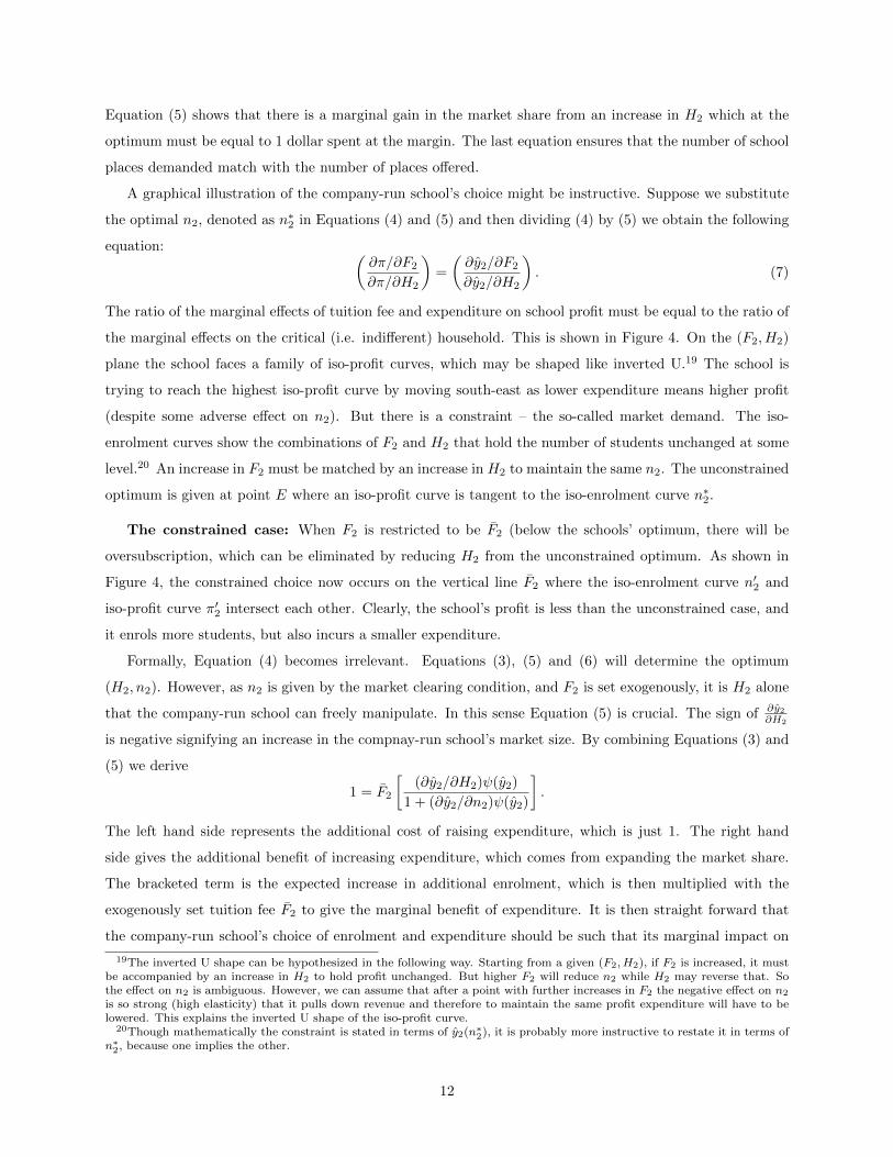
A graphical illustration of the company-run school’s choice might be instructive. Suppose we substitute

the optimal n2, denoted as n∗2 in Equations (4) and (5) and then dividing (4) by (5) we obtain the following

equation: (∂π/∂F2

∂π/∂H2

)=

(∂y2/∂F2

∂y2/∂H2

). (7)

The ratio of the marginal effects of tuition fee and expenditure on school profit must be equal to the ratio of

the marginal effects on the critical (i.e. indifferent) household. This is shown in Figure 4. On the (F2, H2)

plane the school faces a family of iso-profit curves, which may be shaped like inverted U.19 The school is

trying to reach the highest iso-profit curve by moving south-east as lower expenditure means higher profit

(despite some adverse effect on n2). But there is a constraint – the so-called market demand. The iso-

enrolment curves show the combinations of F2 and H2 that hold the number of students unchanged at some

level.20 An increase in F2 must be matched by an increase in H2 to maintain the same n2. The unconstrained

optimum is given at point E where an iso-profit curve is tangent to the iso-enrolment curve n∗2.

The constrained case: When F2 is restricted to be F2 (below the schools’ optimum, there will be

oversubscription, which can be eliminated by reducing H2 from the unconstrained optimum. As shown in

Figure 4, the constrained choice now occurs on the vertical line F2 where the iso-enrolment curve n′2 and

iso-profit curve π′2 intersect each other. Clearly, the school’s profit is less than the unconstrained case, and

it enrols more students, but also incurs a smaller expenditure.

Formally, Equation (4) becomes irrelevant. Equations (3), (5) and (6) will determine the optimum

(H2, n2). However, as n2 is given by the market clearing condition, and F2 is set exogenously, it is H2 alone

that the company-run school can freely manipulate. In this sense Equation (5) is crucial. The sign of ∂y2∂H2

is negative signifying an increase in the compnay-run school’s market size. By combining Equations (3) and

(5) we derive

1 = F2

[(∂y2/∂H2)ψ(y2)

1 + (∂y2/∂n2)ψ(y2)

].

The left hand side represents the additional cost of raising expenditure, which is just 1. The right hand

side gives the additional benefit of increasing expenditure, which comes from expanding the market share.

The bracketed term is the expected increase in additional enrolment, which is then multiplied with the

exogenously set tuition fee F2 to give the marginal benefit of expenditure. It is then straight forward that

the company-run school’s choice of enrolment and expenditure should be such that its marginal impact on

19The inverted U shape can be hypothesized in the following way. Starting from a given (F2, H2), if F2 is increased, it mustbe accompanied by an increase in H2 to hold profit unchanged. But higher F2 will reduce n2 while H2 may reverse that. Sothe effect on n2 is ambiguous. However, we can assume that after a point with further increases in F2 the negative effect on n2

is so strong (high elasticity) that it pulls down revenue and therefore to maintain the same profit expenditure will have to belowered. This explains the inverted U shape of the iso-profit curve.

20Though mathematically the constraint is stated in terms of y2(n∗2), it is probably more instructive to restate it in terms ofn∗2, because one implies the other.

12

the market share is just 1/F2.

Proposition 1. If the tuition fee caps binds, more students are likely to be admitted in the company-run

school relative to the unconstrained case, which indirectly helps to reduce congestion in the public school

and thereby the average test score of the public school will rise. But on the flip side, the expenditure of the

company-run school will fall and so will its average test score α2, relative to the unconstrained case.

Stage 1. The trust school chooses n1 to maximize Z = α1(H1, n1)+w(x) subject to H1 = n1(F1−x)+D,

and n1 ≤ [Ψ(yT ) − Ψ(F1)]. As argued earlier, it is reasonable to assume that the trust is interested in

maximizing average test score and some other social welfare. In so doing it is allowed to decide only on

the number of students it will admit. Its spending on education and socially motivated lessons, as the first

constraint shows, are financed by charitable donations and tuition fees. The second constraint shows that its

students come from families, who are poor but still can afford a small fee. Though the trust school’s choice of

n1 affects the market size of the company-run school as well as the public school, the trust school’s objective

is such that it is unconcerned about these effects.21 Moreover, the second constraint will be non-binding

under the scenario we are considering; hence we can disregard it and incorporating the first constraint we

write the school’s problem as of maximizing Z = α1(n1(F1 − x) +D,n1) + w(x).

The choice of n1 is given by the following first order condition:

Z ′(n1) =∂α1

∂H1(F1 − x) +

∂α1

∂n1= 0. (8)

We assume F1 > x to ensure an interior solution. Maximizing Z is equivalent to maximizing α1. By

increasing n1 the trust is able to raise more revenue and therefore able to spend more, which helps to improve

the averag score, but on the other hand higher n1 also reduces the average score. These two opposing forces

are balanced at the optimum. Thus, we have the optimal n1, which in turn determines n2 and n0 and also

the company-run school’s optimal expenditure and tuition fees.

Insights from our theoretical model: There are several points to note from our simple model.

1. While profit-motivated private schools cater to the high income group, socially motivated organizations,

such as the trust-run schools, can provide a choice to the poor. To what extent that choice will be

superior to the public school depends on the resources available to the socially motivated school.

2. The actions of the trust schools will have a positive consequence for the students of the public school;

the congestion in the public school will be reduced and its average test score will improve.

3. The public school may not necessarily turn into a ‘ghetto’ of the poor; as shown in this model, due

to the presence of the trust school, it may also have a section of the middle class. This diversity may

have some positive effect on the students’ social attitudes.

21Implicitly we are assuming that the private school will set F2 in excess of yT , so that these two schools don’t compete, aswould be realistic for a country like Nepal.

13

4. Though the profit-motivated private school is likely to generate a higer expected test score than the

trust or the public school, by no means it is guaranteed to be the ‘most efficient’ producer of test

scroes. With better infrastructure it has the best technology to produce high test scores; but because

of its profit motive it will also admit more students than socially motivated school (with similar

infrastructure) would. In contrast the trust run school would directly maximize the average test score,

and thus can be more ‘efficient’ user of its limited resources.

In Figure 5 we illustrate this point by drawing two sets of expected test score curves α1 and α2 for

the trust school and the profit-oriented company-run school. Suppose the test score functions are such

that they can be expressed as a function of expenditure per student, h(= H/n), for any given tution

fee and initial capital K. These test score functions have a unique maximum, say α∗1 and α∗∗2 , for the

trust school and the company-run school respectively at h∗1 and h∗∗2 .

The trust school is choosing α∗1 in keeping with its social and educational objective, though α∗1. It is

thus an efficient user of its resources. In contrast, the company-run school will choose h∗2 to maximize

profit, though it could choose h∗∗2 that yields highest test score for its given level of infrastructure.

In this sense, it is not efficinet. Intuitively, it will admit more students to increase its profit. This

deviation from efficiency is exacerbated when the tuition fee cap binds.

5. When the tuition fee cap binds on the company-run school, it is most likely to offer more admissions

and at the same time redue expenditure. Overall, it is reasonable to expect that its enrolment will go

up, which indirectly reduces public school congestion and thus leads to an improvement in the average

test score of the public school; but it comes at the expense of a drop in the average test score of the

company-run school.

6. The question of the expansion of trust schools is also interesting. If more funds are provided to the

trust school, its expected test score will rise via greater expenditure. However, its enrolement may rise

or fall, depending on whether the increased fund helps to ease out the marginal congestion effect. On

the other hand, if the fund is provided to improve the infrastructure of the trust school, then it will

admit more students, which in turn helps the public school. We record this observation in the following

proposition.

Proposition 2. If the fund of the trust school (D), which is used to finance H1, goes up, its expected

score α1 will rise and enrolment may fall or rise. But if the trust school’s infrastructure K1 is improved, then

it will admit more students, and the test score will also rise. In the first (second) case, the public school’s

test score will fall (rise).

Proof: First consider the case of increasing D. That α1 will rise is a straight forward implication of the

envelope theorem. From the trust school’s optimization we get ∂Z/∂D = ∂α1/∂D = ∂α1/∂H1 > 0. For the

14

effect on n1 derive from (8):

Z ′′(n1)∂n1∂D

+∂Z ′(n1)

∂D= 0

or Z ′′(n1)∂n1∂D

+∂2α1

∂H21

(F1 − x) +∂2α1

∂H1∂D= 0

or∂n1∂D

= −∂2α1

∂H21

(F1 − x)

[1

Z ′′(n1)

]< 0.

By assumption ∂2α1

∂H21< 0, and it is reasonable to assume ∂2α1

∂H1∂D> 0. The first negative sign reflects the

diminishing marginal returns to expenditure, and the second positive return reflects diminishing marginal

congestion. Note that ∂α1

∂n1< 0 is the marginal congestion effect. With greater resources, the magnitude of

the marginal congestion effect (|∂α1

∂n1|) should fall, i.e. ∂

∂D |∂α1

∂n1| < 0. Hence, we assume ∂2α1

∂H1∂D> 0.

Also by the second order condition of maximization Z ′′(n1) < 0, and for an interior solution F1 > x.

Then the sign of ∂n1/∂D critically depends on the relative magnitude of ∂2α1

∂H21

, and ∂2α1

∂H1∂D0. So the sign of

∂n1/∂D is ambiguous.

Now consider an increase in K1. As α1 rises with K1, again by the envelope theorem we can argue that

the test score will rise. For the effect on n1 consider as before,

Z ′′(n1)∂n1∂K1

+∂Z ′(n1)

∂K1= 0

or Z ′′(n1)∂n1∂K1

+∂2α1

∂H1∂K1(F1 − x) +

∂2α1

∂n1∂K1= 0.

Since the last two terms in the above equation are positive, the first term must be negative, and as Z ′′(n1) < 0,

we must have ∂n1/∂K1 > 0. QED

In our empirical section we will investigate the households’ school choice and the test score differentials

between schools. Households with higher incomes are expected to choose high end private schools; but to

what extent income plays a role in the choice of a trust school over the public school is of interest. Similarly,

the company run private schools are expected to produce higher test scores, but will they be more efficient

than the trust schools? Also, will the trust schools always be a beter choice than the public school? These

are the questions we will pursue in what follows.

4 Methodological Issues

In this section, we develop an empirical strategy to test our central proposition, after controlling for all other

possible factors so that the omitted variable bias is minimised.

15

Traditional education production functions depict students’ test scores as a function of school and child

characteristics, plus a random term that reflects measurement error in the test score:

Tis = T (scs, fci) + uis (9)

where Tis is the test score of child i in school s, scs is a vector of the characteristics of school s, and fci

are the family and child characteristics of child i, and u measures random noise in the test scores due to the

design of the test and random events that may occur on the day of the test.

Fortunately, in our dataset many of the family and child characteristics are observable; also for school

characteristics we have information on some variables such as the percentage of schools with head teacher’s

full autonomy, students’ access to drinking water and toilet and teachers’ unionisation. However, still the

quality of learning environment induced by the above-mentioned factors is unobservable. So we need to

introduce dummy variables, one for the company-run school and another for the trust-run school (keeping

the government school as the base).22 The significance and size of these two dummy variables would give

the relative efficiency of the two types of the private school, in comparison to the public school.

One of our key innovations is the inclusion of school expenditure per student. Arguably, it contributes to

students’ learning and test scores through its effect of pupils per teacher ratio (as it funds teachers’ salaries)

as well as use various other teaching and non-teaching inputs (e.g., laboratory, library, sports and other

facilities).23 In addition we inlude two dummy variables to control for the company- and trust-run private

schools (relative to the reference category state schools). These school type dummy vairables are meant

to capture differential school specific characteristics as highlighted in Table 1, after controlling for school

expenditure per student. The latter may refer to head teacher’s autonomy, teachers’ efforts, pedagogical

methods, incidence of daily homework and weekly tests, all of which may also influence student performance.

We also include interactions between school expenditure per student and private school type dummies. This

is because the sensitivity of test scores to expenditure per student may not be same in all schools. For

instance, being company run a private school may produce much higher test score on average, but also it

may (or may not) experience an additional effect from expenditure per student suggesting additional benefits

of private management (or the lack of it). Similar argument can be made for the trust school as well. In

fact, whether the trust school differs from the company school in this respect is of great interest. In our

theoretical section we speculated that the company run school may have the highest expenditure per student,

as it caters to the rich, but it may not be the most efficient user of resources as far as the test scores are

22Otherwise, the unobserved components of scs and fci will end up in the error term. This will result in the error termbeing correlated with the observed school and child characteristics, producing biased results. Needless to if all the schoolcharacteristics were observed, the dummy variables would be insignificant.

23There is, however, a controversy about the effect of school resources on student achievement in general. Hanushek (1997)concluded that ’there is no strong or consistent relationship between school resources and student performance’. This pessimisticassessment has however been challenged by other US researchers, in particular Krueger (2003), who has criticised Hanushek’smethods of selecting studies for review and interpreting them; they provide contrasting evidence of a positive relationshipbetween resources and student attainment, thus justifying a scope for further study. As such there is a need to empiricallyre-examine the role of school expenditure per student on test scores. We also test the robustness of our expendiure resuls indifferent ways.

16

concerned. To the best of our knowledge, incorporating these issues in a school efficiency analysis is a novel

attempt in addition to comparing three types of schools.

Two school dummies are S1 for trust run schools and S2 for company run schools, so that the government

schools form the reference category. The school expenditure per student is denoted as sx that covers the

running expenses of various teaching and non-teaching inputs in each school type. In order to capture the

differential expenditure effect, if any, for each type of private schools, we also construct two interaction

terms between school expenditure per student sx on the one hand and school types S1 and S2 on the other.

Accordingly, we can express characteristics of the school attended by the i-th child as follows:

sci = f(S1i, S2i, sxi, sxi ∗ S1i, sxi ∗ S2i) (10)

Thus after substituting for sci from equation (10) into equation (9) for all schools taken together, the

total score of the i-th child in our sample would be given as follows:

Ti = F (S1i, S2i, sxi, sxi ∗ S1i, sxi ∗ S2i, fci) + uis (11)

Finally for estimation purposes, we approximate equation (11) by the following linearized equation to

determine test score of the i-th child:

Ti = b0 + b1S1i + b2S2i + b3(sxi) + b4sxi ∗ S1i + b5sxi ∗ S2i + γ(fci) + ui (12)

The parameters of particular interest to us are the estimated coefficients of the two interaction terms

sxi∗S1i and sxi∗S2i, which determine the expenditure efficiency of trust-run and company-run private un-

aided schools (relative to fully funded government funded schools) respectively for a given level of school

expenditure per student.

The fact, however, remains that children who attend private schools may differ in unobserved ways from

children who attend public schools. For example, parents who send their children to private schools may also

help their children, or require them to study more, compared to parents who send their children to public

schools. This is the problem of selection bias, which may render simple OLS estimates of (11) to be biased.

Hence we need to correct for this selection bias, which is explained in the next sub-section.

4.1 An Empirical Model

We start with the school choice equation for the i-th child from the j-th household residing in the k-th VDC

(municipality)24 as follows:

24This is identified by the village development committee or VDC for short in our sample, which is the lowest administrativeunit for Nepal’s local development ministry. Each district has several VDCs, similar to municipalities but with greater public-government interaction and administration

17

Y ∗ijk = a0 + a1Ak + a2Wijk + uijk. (13)

While Y ∗ is unobservable, it is related to an observable variable S, which takes a value 1 if the child

goes to a company-run school, 2 if the child goes to trust-run school and zero otherwise.25 The explanatory

variable A takes a value 1 if there is a government school in the k-th VDC (i.e., municipality) where the

child resides, and 0 otherwise. It can be argued that the access to a government secondary school Ak in the

municipality is a purely exogenous variable, as the presence of the school in the VDC determined by the

government and as such is beyond the control of the child/child’s family. Clearly presence of government

school in a municipality is closely related to parental school choice and, without much loss of generality,

we can therefore treat it as an exogenous determinant of his/her private school choice/enrollment. As high

as 92% (71%) of sample VDCs have a governent (private unaided) secondary school in the vicinity so that

access to government schools in the community is an essential part of parental school choice decision 26

The set of variables, W , on the other hand, includes a set of individual (e.g. gender, age) and household

(e.g. parents’ education, income and caste) characteristics relevant for the school choice equation. Given

the discrete nature of the dependent variable in equation (13), we use a multinomial logit model to estimate

the parameters of equation (13), which are then used to generate the inverse Mill’s ratios MGOV , MCO and

MTR respectively for government, company and trust-run private school choice in our sample.

At the second stage these inverse Mill’s ratios (MGOV , MCO and MTR) are included in the estimation

of equation (11) that determines the total test scores T (a la Lee 1983). Total test score Tijk of the i-th

child from j-th family living in k-th municipality is determined in terms of school expenditure per student

EXP, school type (CO and TR) and also interactions between EXP and school type (CO and TR). In

view of the non-linear relationship between standardised test scores and school expenditure per student as

seen in Figure 1, we use natural logarithm of the continuous school expenditure per student and denote it

by lEXP . In doing so, we control for various individual/ family characteristics (fc) and unobserved VDC

characteristics (ϕk) that account for the unobserved VDC-level variation in public infrastructure, returns to

schooling, culture, which could also influence students’ test scores.

25Note that our baseline regressions exclude private aided schools from the analysis; thus the reference category is the fullyfunded government schools. However, in section 5.5 we relax this restriction and examine if our central hypothesis holds evenafter we include private aided school as a separate category in school choice equation.

26We have also considered the presence of private secondary schools in the municipality as an alternative instrument; butchose not to include it because it is potentially endogenous. Presence of a private school in a community is a matter ofpreference and lobbying of the local community population. In contrast, presence of a government schools is more likely to bedetermined by the people outside the community. Further, we find that the local access to a government secondary school doesnot significantly influence total test scores while that of a private secondary school boosts student standardised test scores. Assuch we chose acces to local secondary government schools to be an exogenously given identifying variable in the determinationof private school choice in the community and not in the 2nd stage test score equation.

18

Tijk = β0 + β1COijk + β2lEXPijk + β3COijk ∗ lEXPijk + β4TRijk

+β5TRijk ∗ lEXPijk + β′fcijk + βGMGOV ijk + βCMCOijk

+βTMTRijk + φk + eijk (14)

Among individual/family characteristics (fc), equation (14) includes characteristics of the child (male,

age at SLC, square of age, if received any peer group help, if no grade repetition in year 9, which is a measure

of unobserved ability of the student), those of the family (if any family member is at least a graduate and

household expenditure decile). We would also like to run this model for rural urban regions separately.

Note that access to a government school variable A is excluded from the test score equation (14), because

it is unlikely to have a direct influence on SLC test scores. As such the variable A acts as an identifying

restriction for the selection equation. Note that equation (14) is an augmented version of equation (12) in

that it controls for the possibility of selection bias in the test score estimates arising from the choice between

government and private schools. The latter is reflected in the inclusion of the three Inverse Mill’s ratios

(IMR) respectively for the government (MGOV ) and two types of private schools ( MCO,MTR) schools (a

la Lee, 1983). As such, the estimates of equation (12) would entail the uncorrected estimates while that for

equation (14) would yield the corrected estimates of test scores.

We also consider different variants of equation (14) to understand the role of expenditure: (i) first we

only retain lEXP and drop the private school dummies and their interactions to lEXP - this enables us

to understand to what extent school expenditure per student accounts for school efficiency, other factors

remaining unchanged. (ii) Next we augment specification (i) by adding the interactions betweeen lEXP

and private school dummies with a view to understand the differential effect of expenditure per student by

private school type. Note that in this case we do not include the private schools dummies on their own.

(iii) Finally, we also estimate equation (14) that includes lEXP , private school dummies and interactions

of lEXP with private school dummies. The latter is the most complete specification and hence is our

preferred option. The coefficient of particular interest to us is that of the interaction term between the

private school type and log expenditure per student, which captures the efficiency of the particular type of

private school per unit of school expenditure per student, after controlling for student ability/motivation,

household income/education, and/or other unobserved community characteristics that may also influence

student test scores.

4.2 Econometric issues

Unlike the literature on school resources and student outcome (Hanushek, 1997; Krueger, 2003), our analysis

focuses on private unaided schools and hence the case of government allocation of funds to schools does not

arise. Similarly, our case is different from the cases of government schools in the US and the UK (e.g., see

19

Steele et al. 2007) as school funding is not a function school performance. Nevertheless head teachers would

care about school performance in both trust and company run schools, but more so in trust-run schools.

Accordingly, we consider two possible sources of omitted variables. The first one arises from parental

demand for better performing schools. An obvious solution would be to exploit the intra-household variation

in school choice and student performance, if possible; but we were unable to do this as we did not have SLC

information for all the siblings living in a household. Hence, we control for various parental characteristics

including education, income and caste. We also control for the unobserved community level (i.e., VDC)

characteristics which determines households’ access to different types of schools, as long distance travelling

to attend better performing schools is not so common in Nepal27. As an alternative, we also generate a pseudo

panel for each individual with test scores across six compulsory SLC subjects with a view to determine the

subject fixed effects estimates of standardised test scores. The latter allows us to exploit the variation across

subjects test scores (standardised) for a given individual, thus eliminating individual/household level time

invariant unobserved factors that may also influence test scores.

A second source of estimation problem arise from schools’ (by type) efforts to perform better and thereby

investing/recruiting teachers/students of highest ability. The latter may give rise to the potential simultaneity

of school expenditure (as well as teachers’ salary) per student while determing test scores.While contemporary

expenditure per student could be endogenous to test scores in the same year (and may not also fully account

for performance as performance improves over time especially during year 9-10), we consider 3 years average

expenditure (as well as salary) per student for the period 2002-04 at our access, which is a more long-term

measure and may minimise the potential simultaneity while determining SLC test scores.

Note that we were unable to use school fixed effects estimates as we aim to compare and contrast students

across private school types - trust or company-run. Hence all regressions control for school expenditure

per student (2002-04 average), school type (trust indicated by pua sch tr or company schools indicated by

pua sch co) and also an interactions between the two. So long as we control for pua school type dummies,

we account for pua school type level unobserved factors (for example, teacher’s quality or characteristics

of school management) that may influence student test scores. But there could also be unobserved time-

varying school type level factors (e.g., change in school management or change in teachers or non-teaching

staff) exclusion of which may give rise to endogeneity bias as well. Given that we have access to 2002-2004

SLC test scores, we account for school type level unobserved time trends as captured by pua sch trust*slcyear

and pua sch co*slcyear (e.g., see Appendix Table A3).

All estimates are clustered around school id-s with a view to minimize any cross-correlations in the error

terms for students attending a given school. We obtain the corrected standardised test score estimates not

only for the latest survey year 2004, but also for the entire period 2002-2004; in the latter case, we also

control for the SLC year fixed effects and also pua school type-level unobserved SLC time trends (e.g.,

examination related factors overall or school type specific exam related factors) that may also influence SLC

27as high as 90% of sample students stayed with parents and another 3% or so stayed with relatives during year 10

20

test scores. We check the robustness of our estimates in different ways to eliminate competing explanations:

(i) We compare the effect of school expenditure per student by replacing school expenditure per student

by teachers’ salaries per student and also pupils-teacher ratio. (ii) We also obtain the subject-specific fixed

effects estimates of test scores for both 2004, as it allows us to identify the effect of school type on subject

level test scores by exploiting the variation in test scores across 6 compulsory subjects for each student and

as such better eliminates household/student-level time-invariant omitted factors, if any. (iii) We also try to

eliminate the effect of private tuition on standardised test scores as far as possible with a view to establish

that our results are not an artefact of differential levels of tuition among students attending these three types

of schools.

Means and standard deviations of all explanatory variables are shown in Appendix Table A1.

5 Results

This section presents and analyses various estimates of school choice and standardised SLC test scores that

we obtain from our sample .

5.1 School choice

Table 4 summarises the first stage multinomial logit marginal effects estimates of choice of fully funded

government and two types of private schools. Columns 1-2 show the estimates for 2004 while columns 3-4

show those for 2002-04. For each period, we show the estimates for company-run (columns 1 and 3), trust-run

(columns 2 and 4) private schools (reference category being the government schools).

We use the presence of a fully funded government school in the community as an identifying variable for

the school choice equation. It can be argued that the presence of a local government school is exogenously

determined by government authority and as such their presence is beyond the control of private households in

the community. Further, we find that the local access to a government secondary school does not significantly

influence total test scores and hence we chose it to be an exogenously given identifying variable in the

determination of private school choice in the community and not in the 2nd stage test score equation. We

also control for individual age, gender, household caste, expenditure, and community dummies (as captured

by VDC) to control for unobserved community factors that may also influence school choice. Ceteris paribus,

results suggest that the private school enrolment is higher in the presence of a fully funded government school

in the community. Further, this effect is statistically significant only for the company run private school and

not for the trust-run private schools. In other words, trust schools’ admission policy is different, as we have

assumed in our theoretical section.

Second, we consider the estimates of household expenditure decile where a higher value of the household

expenditure corresponds to significantly higher likelihood of private school choice irrespective of their type

21

(i.e., trust or company run schools). In other words, students from richer (i.e., from higher expenditure

deciles) households are significantly more likely to choose trust and company run private schools and thereby

less likely to choose fully funded government schools. Also note that the marginal effects of household

expenditure deciles are quite comparable for choice of trust and company run schools, if both are available in

the community, among children from richer households so that they do not reveal any significant preference

for company run as opposed to trust-run private schools. In a similar vein, we find that children from Dalit

(i.e. lower caste) households, who are also poor, are less likely are more likely to be enrolled in private

unaided schools. This pattern tallies with our theoretical model. Individual age or parental education does

not turn out to be very important here. Among other variables, boys are significantly more likely to choose

private schools irrespective of their type, thus suggesting a male bias in parental school selection. We obtain

similar results irrespective of the year under consideration. Results are similar irrespective of whether we

consider only 2004 or 2002-04 sample. There is some evidence that children from rural areas are less likely

to go to any type of private schools during 2002-04.

5.2 Private school premium

We use the first stage multinomial logit estimates (obtained from Table 4 estimates) to generate the inverse

Mill’s ratios (IMR) for the choice of fully funded government and two types of private schools in our sample

for both 2004 and also for the entire 2002-04 periods. Following Lee (1983), we include these three IMRs

to determine the standardised test score estimates in the second stage to corrected for the selectivity bias.

Table 5 shows the standardised test score estimates in 2004 (columns 1 and 2) and also 2002-04 (columns

3 and 4). Columns (1) and (3) show the uncorrected test score estimates while columns (2) and (4) show

the selectivity corrected test score estimates. Since the inverse Mill’s ratios for both government and private

school choice are statistically significant, we couch our discussion in terms of the corrected estimates of test

scores.

We first note that certain individual and household characteristics matter. For instance, male students

perform better, and with higher age some increasing returns also set in. Peer help positively affects the test

score and conversely ill health hurts. Parents with graduate or higher education are also a facilitating factor.

However, household incomes do not matter.

Here is an issue of student’s ability. It is very difficult to get data on this. However, we use one piece of

information that reflects student’s ability to some extent. There are students in our sample who had repeated

grade nine. If they did not do this on medical ground (which we have controlled for by the illness variable),

then they must be academically weaker students than those who did not repeat grade nine. Column 2

estimates show that those, who did not repeat grade nine, scored 9.11% standard deviation higher than

those who did.

Now we turn our attention to the question of school premium. From the significance of two private school

dummy variables, it is clear that there is substantial premium for both types of private schools. Further,

22

the coefficient of the trust school dummy is higher than the coefficient of the private school dummy in all

four regressions. This is true regardless of the year and whether or not the selectivity bias is corrected. In

all cases the trust school is the most efficient of all. The premium for the trust school is even higher when

the entire time period 2002-04 is considered (column 4).28

Next question is where this efficiency comes from. Is it the learning environment specific to a company-

run or trust-run school (as captured by the private school type dummy), or is it due to the expenditures

made by particular private school management toward teaching staff and non-teaching resources (as captured

by the interaction between private school dummy and log expenditure per student)? Company-run schools,

being profit maximizers, will naturally be efficient users of resources toward providing a more disciplined

environment. Trust-run schools, on the other hand, are socially motivated and may be directly geared toward

test score maximization. Therefore, when other factors are controlled for, social objective alone may turn a

school most efficient. However, we still need to see whether the source of efficieny is something intangible or

something measurable like school expenditures per student. We address this next.

5.3 School expenditure and private school premium

We add log expenditure per student (3 years’ average) to the set of explanatory variables. Table 6 reports

these estimates. Columns (1)-(3) show the estimates for 2004 while columns (4)-(6) show those for 2002-04.

As the estimates are similar, we can restrict our discussion to 2004. We first see the effect of log expenditure

without taking account of the school types in column 1 (and likewise in column 4). This effect is positive

as expected. Next, we add the school dummies, but only as interaction with the log expenditure. The

direct effect of expenditure immediately disappears; expenditure matters only if it is a trust-run school or a

company-run school. That means, in government schools expenditure has no effect. Between the two private

schools, the company-run schools seem to be more efficient user of expenditures.

But when we add the private school dummies too in column 3 (most complete specification), the relative

superiority of the company-run schools is threatened. The private school dummy is significant, but its

interaction with log expenditure loses significance. Just like the government run schools, expenditure does

not have any additional impact in company-run schools; it is the learning environment of a company-run

school, presumably made possible by expenditure, that counts the most. We know that the company-run

schools are better managed with great deal of focus on discipline. The head teachers in these schools

have greater autonomy and teachers are less unionsied. These facts alone may contribute a lot to student

achievement.29

But for the trust school, its dummy does not become significant, while its interaction with log expenditure

28A comparison of the corrected estimates with the corresponding uncorrected ones suggests that the uncorrected estimatestend to under-estimate the private school premium.

29A striking difference among the three types of schools in Nepal is the variation in head teacher’s autonomy in discipliningteachers. While on average 81% of company run private school heads have this autonomy, the corresponding proportion falls to49% for government schools and 44% for trust-run private schools.Although we do not explicitly control for these differences,we argue that the two private school dummies would account for these differences in our model.

23

turns out to be significant. That is to say, the status of being trust-run or government-run does not make

any difference to test scores. In principle, both the trust-run and the public school would be sharing a

common social objective, and therefore, being trust-run per se may not make any difference. However, the

trust school has the advantage of being wastage free. Therefore, it will be able to utilise additional fund

much more efficiently than the public school. This is why the expenditure incrementally improves the test

score in trust schools (reference category being government schools).

An intriguing possibility is that with the positive incremental effect of expenditure the trust school’s test

scores will rise, and potentially can exceed the company-run schools’ test scores if the expenditure exceeds

a critical level. Indeed, using column (3) data we can write the test score equation (suppressing all other

variables) for the trust school as TT = 2.101 + 0.829x where x is the log expenditure per student. For

the company-run schools, where expenditure has no incremental effect, the test score equation is simply

TC = 3.236. If x > 1.369 or equivalently if the annual expenditure per student exceeds 3931.88 Rupees, the

trust school will produce higher test scores than the company run schools. According to Table 1, the mean

(annual) log expenditure per student is 3.714 Rupees for government schools, 5.263 Rupees for trust schools

and 6.966 Rupees for company-run schools. Therefore, a large number of trust schools are likely to be more

efficient than the company-run schools. On the other hand, at lower level of expenditures, company-run

schools are most efficient.

So long as we control for school type (trust and company-run private schools), we account for school

type level unobserved factors that may influence student test scores. For example, teacher’s quality, nature

of school management that may influence investment in school infrastructure. But there could also be

unobserved time-varying school type level factors (e.g., change in school management or change in teachers

or non-teaching staff) exclusion of which may give rise to endogeneity bias as well. Given that we have access

to 2002-2004 SLC test scores, we further try to account for school type level time trends as captured by

pua sch trust*slcyear and pua sch co*slcyear. These estimates (see Table A3) are also generally compatible

with the baseline results shown in columns (4)-(6) of Table 6.

Some policy makers have advocated in favour of low-fee private schools (e.g., Tooley and Dickson, 2003).

In an attempt to see how low-fee company schools perform vis-a-vis trust schools in our sample, we next

distinguish between low and high fee company schools as follows. A company school is defined low fee if

its monthly tuition fee per student in year 10 (the final year before the SLC exam) is less than the first

quartile value (Rp 850) in its distribution. This contrasts with an average monthly tuition fee of Rp 1200

for trust schools and 0 for government schools for year 10. These resutls are summarised in Table 6A. After

controlling for all other factors, we find that expenditure efficiency of trust schools still holds for both 2004

and 2002-04. For 2004, the expenditure interaction term insignificant for low-fee company schools while it is

is positive and significant for both trust and low fee schools in 2002-04; however the size of the interaction

coefficient is still higher for the trust schools.

24

5.4 Rural-Urban differential in school premium

But is the hierarchy of private schools (conditional on expenditure) valid in all regions? We try to answer this

question by disaggregating the data for rural and urban regions. Table 7 shows that there are interesting

differences between the rural and urban parts of Nepal. We run the same set of regressions as shown in

Table 6, except that we restrict only to 2004 data. For brievity we just report the findings of the augmented

regressions shown in columns 3 (rural) and 6 (urban).

The findings are summarised in Figure 6. As seen in Table 6, here too expenditure does not have any

incremental effect on any type of schools except the trust school; this result is robust in both regions.

However, the hierarchy between three schools is not same between the ruran and the urban regions. In the

rural region, at low levels of expenditure, i.e. log expenditure below 0.899 or equivalently annual expenditure

per student less than 2457.90 Rupees, the company-run school is most efficient, followed by the public school

and the trust school coming last, as shown in panel a of Figure 6. But as the trust school is able to increase

its test score by 1.013 standard deviation for an extra unit of log expenditure, it outperforms the public

school from the log expenditure of 0.899 onward, and eventually overtakes the company-run school from

1.522 log expenditure (or equivalently, 4582.347 Rupees) onward. Thus, at higher levels of expenditure the

trust school is a clear winner.

In the urban areas, as is evident from column 6 estimates, the public school is always at the bottom.

Between the two private schools, the trust-run school overtakes the company-run school at log expenditure

of 1.551 or equivalently 4720.128 Rupees onward, which we depict in panel b of Figure 6. Thus, the ordering

of the two types of the private schools is similar between regions.

Here we may recall from Tables 3 and 3A that rural trust schools spend much more per student per

year than the rural company-run schools – 6600 Rupees as opposed to 4820 Rupees. In the urban sector,

however, the company-run schools spend nearly twice as much (9070 Rupees), while the trust schools spend

only 4940. So in the urban areas the company-run schools are able to hold on to its superiority a somewhat

longer until the expenditure reaches 4720.18 Rupees.

It is well known that profit motivated schools spend substantially on infrastructure or nonteaching facil-

ities often to attract rich households. These facilities may be valued by well off families for social or other

purposes, but they may not contribute much to test scores. It may also be the case that part of the ex-

penditure is directed to monitoring teachers, and enforcing student disciplines; but as these things form the

key characteristics of company-run schools their effect is felt only through the school dummy. On the other

hand, the trust-run schools are socially motivated and directly aiming at maximizing student achievements.

This social objective can be a powerful driver of using every available resource to their best use. Therefore,

one may argue that if external funds are to be provided to any of the schools, they should be given to the

trust schools, because they are the most efficient user of expenditures.

Role of teacher’s salary: We can probe this issue further by considering the spending on teachers’

25

salary per student, which constitutes 80% of the total expenditure in public schools, 70% in company run

schools and 72% in trust schools. From Table 1 we see that the salary per teacher is highest in public schools

(179000 Rupees per year), closely followed by the company run school (165000 Rupees), with the trust

schools coming a distant third (117000 Rupees). The company run schools maintain the best pupil teacher

ratio (18 pupils per teacher), while the trust schools have 26 pupils per teacher; but the public schools, not

unexpectedly, have many more students (42) per teacher. We replace log expenditure per student by log

salary per student and run the same regressions as in Tables 6 and 7. Estimates of these regressions are

given in Table A2 in Appendix.

Column 1 of Table A2 reports the estimates for the whole country, while columns 2 and 3 report the

estimates for urban and rural sectors respectively. The results are consistent with Tables 6 and 7. Log salary

is significant only in trust schools, just as the total expenditure was. Since salary is on average very low in

trust schools (34.63% less than the public school), and therefore, teachers respond much more positively to

salary rises. In addition, these teachers are more likely to share the ideology of the school, and they are also

likely to be socially motivated. In contrast, teachers in public schools are probably neither motivated, nor

easy to monitor (for being unionised). Teachers in private schools, however, are more closely monitored as

their Head teahers have greater autonomy in managing them. Therefore, it is not the salary but the Head

teacher’s role that is more important in private schools. As in Tables 6 and 7, the trust schools come on top

at higher levels of log salary, and the company run schools come on top at low levels of log salary. However,

in this case, neither in the rural sector (column 2) nor in the urban sector (column 3) the trust school ever

comes last. It is as good as the public school, if not better.

5.5 Ruling out competing explanations

We now try to rule out some competing arguments for private school premium. The first argument relates

to the fact that the expendiure data may not be reliable and that the effect of expenditure on performance

could be ambiguous (a la Hanushek, 2003). In order to address these concerns we replace expenditure by

pupil-teacher ratio which is a reflection of school expenditure. The second one concerns the unobserved

student characteristics, e.g., his/her subject preference (or the lack of it) which may bias our estimates. If

students had a particular subject preference, then her test score might be less (or more) affected by the

school’s teaching. We address this concern by considering subject fixed effects estimates, as we exploit the

variation in student performance across six compulsory SLC subjects. Further, there are growing concerns

about the use of private tuition in many emerging economies. The students’ test scores might be affected

by extra-school tuition received, in which case the estimate of school preimum might be upwradly biased.

In our main regressions (Tables 5-7) we did not include private tutoring as a separate explanatory variable,

because the demand for private tutoring is likely to be correlated with the school’s expenditure. If a school

spends more on teaching, then its students should feel less compelled to seek outside tutoring. Further there

is likely to be a simultaneity between tutoring and test scores. We try to address these concerns in two ways

26

– first by explicitly including past private tuition as an explanatory variable for determining standardised

SLC test scores, and then by focussing only on those who did not take private tuition (which reduces the

sample size). Finally, so far we did not include the case of private aided schools in our analysis,which operate

very similarly to government funded schools in many ways, with a view to compare fully funded government

schools with trust and company run schools. We shall now relax this assumption with to examine if their

inclusion would alter the relative efficiency of trust schools.

5.5.1 Pupil-Teacher Ratio

One may argue that the total salary and/or expenditure data may not be reliable. Further there is a debate

about the role of expenditure on student performance (Hanushek, 2003; Holmund et al. 2010). In an attempt

to address these concerns, we replace expenditure by pupil-teacher ratio, which is effectively an outcome of

expenditure incurred by schools and certainly a hard data. Table A4 shows these estimates. Not only do we

see the same pattern of efficiency among schools that we have seen earlier, but the superiority of the trust

school now becomes unconditional and quantitatively stronger. The dummy variable for the trust school is

3.594 (for 2004 data), while the same for the company run school is 0.75. So the trust school leads to a more

than 4 times standard deviation higher score than the company run school. A higher pupil-teacher ratio

reduces test score only in the trust school, very much like the expenditure or teachers’ salary exerted their

desired effects on the test scores only in trust schools. These estimates further establishes the robustness of

the estimates shown in Table 6.

5.5.2 Subject fixed effects

Given the richness of our dataset we are able to control for a range of individual, household, community and

school characteristics in a rigorous way and minimize the omitted variable bias with a view to identify the

causal effect of school choice on performance and also the underlying mechanism. Still there may be a bias

from other omitted variables (e.g., parents/students’ preferences for better performing schools or student

preferences or lack of preference for a subject), which could be correlated with the error term. Given that

it is not possible for us to have school-level analysis (as we want to compare/contrast student performance

by school types) or student-level panel data for the SLC test scores for non-repetitors, we rearrange the

student-level data for 2004 to generate subject-level scores for six compulsory SLC subjects for each student,

which can be treated as a pseudo panel. This allows us to exploit the inter-subject variation in standardised

SLC test scores for a student and in the process eliminates household/student-level time-invariant omitted

factors, if any, affecting test scores.

The subject fixed effects estimates of standardised test scores for 2004 are summarized in Table 8 ; the

corresponding school choice estimates for this sample are summarised in Appendix Table A5. As before, we

cluster all errors at the school level to minimize any bias arising from the cross-correlation of errors for a

given school. Since IMRs are statistically significant, we shall, as before, couch our discussion in terms of

27

these corrected estimates. Since there are six compulsory subjects for which we consider the students’ test

scores, the number of observations is six times that in Table 6 column 3.

The model we regress is also similar to the one reported in Tables 6 and 7. Column 1 of Table 8 shows

the regression for all students; columns 2 and 3 are for the rural and urban regions respectively. As can

be seen the pattern of school premium is same as in Table 6 and 7. The regional patterns are identical to

that seen in Table 7. For the national case, the picture closely resembles more like the rural region with the

trust school coming last at low levels of expenditure. Therefore, we can argue that our baseline estimates

are fairly robust.

5.5.3 Estimates for students with and without private tutoring

As is well known, the market for private tutoring is rife in many developing markets and Nepal is no exception.

As shown in Table 1, private tutoring is common among all students irrespective of the school type, though

its prevalence is about 10 percentage points higher for students in government schools. However, private

tuition variable is unlikely to be random in determining test scores and hence we did not directly include it

as an explanatory variable in our baseline regressions (Tables 5-7). Here, we examine if inclusion of private

tuition alters our estimation results and in this respect we conduct two sets of regressions: first we include

a dummy for private tuition undertaken in the past 6 months before the SLC examination for the whole

sample (column 1 of Table 9) and secondly we consider only those students who did not take any private

tuition (column 3 of Table 9). Of course the number of observations drops drammatically in the second case.

Each regression is repeated for subject test scores (cloumns 2 and 4 of Table 9).

A surprising finding of Table 9 is the negative sign of private tuition. One possible explanation for this

is that where students take private tuition, the teachers underperform at school and this substitution of

class-room effort may hurt the student, in the form of an overall loss of learning. It may also be the case

that the students fail to learn independently when they receive extra help, which affects their test score

eventually. See Jayachandran (2008) for a similar result obtained in the context of Nepal.30 However, for us

it is heartening to see that the pattern of school premium remains in tact, which is evident from columns (1)

and (2). There is a private school premium, but there is also no clear winner. The trust school dominates

at a higher level of expenditure.

Next we exclude all students who had private tuition. Once again the result remains in tact. Interestingly,

the picture (as given by column 3) resembles that in panel a of Figure 6, as there are two critical levels of

expenditure. Below the first critical level of expenditure the trust school comes last, and above the second

critical level of expenditure the trust school comes on top. The government school comes as moderately

efficient, particularly at low expenditure levels. This picture is valid also when we study the subject level

test scores (column 4). Since in this subsample no students had been tutored privately, the school dummies

capture the school’s effect much more precisely, and we see that the pattern we saw earlier remains valid.

30Jayachandran (2008) mainly focusses on private tutoring and in many cases school teachers tutor their own students. Sheuses the same data as ours.

28

It is also noteworthy that the company-run school’s premimum over and above the state schools is much

more pronounced here – 1.437, as compared to that in column 3 of Table 6 (1.135). In fact, the difference

between the company-run school and the trust-run school is also widened. Based on the estimates of column

3, we can write the trust-run school’s test score equation as ST = −2.395 + 1.607x, while the company-

run school’s corresponding equation is SC = 1.437. These two lines cross at x = 2.380, or equivalently

at an expenditure of 10807.19 Rupees. This is significantly higher (more than doubled) than the critical

expenditure level we have seen earlier (see the discussion in reference ot Table 7). This suggests that if

there were no private tuition provided at all, still we would get the same hierarchy of schools, but for the

trust school to come on top its expenditure must rise significantly above its current level. In fact, given

the current level of spending, the private school would have maintained its supremacy, if no private tuition

were provided. This is consistent also with our primarly observation that the company-run school students

receive less private tuition than others.

5.5.4 Role of private aided schools

Table 10 summarises the total standardised test score estimates for 2004 and 2002-04 when we include

private aided schools as a separate category. The corresponding school choice equation estimates are shown

in Appendix Table A6. Evidently the estimated coefficient of private aided school dummy PA sch is negative

(and insignificant) on its own; also the estimated coefficient of PA sch dummy is insignificant when it is

interacted with log expenditure per student. There is thus no evidence to suggest that students graduating

from private aided schools perform any better than fully government funded schools (reference category).

As before, the company school dummy is significant and positive on its own while the trust school dummy is

significant and positive when interacted with log expenditure per student. In other words, our central results

are robust to inclusion or exclusion of private aided schools and there is further confirmation that socially

motivated trust schools are most expenditure efficient among all types of private schools in our sample.

6 Concluding Comments

This paper utilises a unique database from Nepal to determine if there is private school premium, and, if so,

to what extent the profit motive contributes to the premium. There are broadly two types of private schools

in Nepal: profit-motivated company-run schools and socially motivated trust-run schools. In general, the

company-run schools are more expensive, spend more per student, and also generate higher test scores at the

school leaving exams. Trust-run schools, though fewer in numbers, seem to be following the company-run

schools. Both of course are ahead of the state-run schools. But when we control for individual and household

attributes, and focus on the school characteristics, we see a different picture. When the school premium is

determined considering only the school type, the trust school comes on top, slightly but distinctly, ahead

of the company-run school; both types show substantial premium over and above the government schools.

29

Further, when we include the school’s expenditure per student, we see that expenditure has incremental

effects only in trust-run schools; but that comes with a fall in the trust school’s intercept. Consequently,

the hierarchy of the three types of school is sensitive to the expenditure level they choose. At high levels of

expenditure, the trust schools are the winner, and at low levels of expenditure the company-run schools are

the winner. More importantly, the government-run schools are not always the loser. This picture is fairly

robust across regions (rural or urban), to considerations of subject fixed effets and to inclusion or exclusion

of private aided schools and private tution.

Our analysis gives two important messages. First, socially motivated schools can outperform both profit-

motivated schools and the government schools. That is to say, what is seen as pro-poor philanthropic activity

can have a strong efficiency dimension. Second, more funds should be directed to such socially motivated

schools. Though they are privately organized, by freeing themselves of the profit motive, they would put

money where the mouth is; they would spend on educational improvements. A profit-motivated school may

decide on its spending strategically, to attract more students, or to improve its sporting and extra-curricular

activities, and thus compromise on the efficient use of resources. Government schools, which are supposed

to be socially motivated, are hamstrung by wastage and bureaucracy.

There is yet another implication of our study. Education is important for peace building through social

inclusion and cohesiveness, especially in a country like Nepal which suffered more than a decade from civil

conflicts. Despite huge investment in public schools, the performance of students graduating from public

schools significantly lags behind their cohorts from private schools. Socially motivated schools can provide a

good alternative, especially to the poor parents, promising a better future for their children, who would have

otherwise joined the rebels. Education can be a great peace builder. We hope our findings will inform the

donors and policymakers in poor countries that are trying to rebuild themselves after suffering a prolonged

armed conflict.

30

References

[1] Beegle, K. and D. Newhouse. 2006. The Effect of School Type on Academic Achievement: Evidence

from Indonesia, Journal of Human Resources 41(3):529-557.

[2] Besley, T. and M. Ghatak. 2007. Retailing Public Goods: The Economics of Corporate Social Respon-

sibility, Journal of Public Economics 91:1645-63.

[3] Bhatta. S. 2005. Determinants of Student Performance in the SLC Examinations’, SLC study report

13, Ministry of Education and Sport, Nepal.

[4] Caddell, Martha (2007). Private Schools and Political Conflict in Nepal. In: Srivastava, Prachi and

Walford, Geoffrey eds. Private Schooling in Less Economically Developed Countries: Asian and African

Perspectives. Oxford Studies in Comparative Education. Didcot, UK: Symposium, pp. 187-207.

[5] Carney, S. and M.B. Bista (2009). Community Schooling in Nepal: a genealogy of education reform

since 1990. Comparative Education Review, Vol. 53, No. 2, 2009, p. 189-211.

[6] Chudgar, A. and Quin, E. (2012) Relationship Between Private Schooling and Achievement: Results

from Rural and Urban India. Economics of Education Review, Vol. 31: 376-90.

[7] Dahejia, R., T. DeLeire, E. Luttmer and J. Mitchell. 2007. The Role of Religious and Social Organiza-

tions in the Lives of Disadvantaged Youth, Kennedy School Research Working Paper RWP07-037.

[8] EdInvest (2000), Investment Opportunities in Private Education in India, International Finance Orga-

nization, available online at http://www.ifc.org.

[9] Epple, Dennis and Richard E. Romano. 1998. Competition between private and public schools, vouchers

and peer-group effects, American Economic Review, 74(1): 33-62

[10] Gautam, R. (2008). Samtaka dhristile niji biddhyalaya [Private schools and equity]. In J. Subedi (Ed.),

Kasima niji biddhyalaya [Assessing private schools] (pp. 47–60). Kathmandu: Education Journalists’

Group and Action Aid, Nepal.

[11] Government of Nepal: Ministry of Education. (2009). Compendium on education policy in Nepal.

Kathmandu.

[12] Hanushek, E. 1997. Assessing the effect of school resources on Student Performance: An update’,

Educational Evaluation and Policy Analysis, pp. 141-164.

[13] Hanushek, Eric A. 2003. The failure of input-based schooling policies. Economic Journal 113(485):

F64-F98.

[14] ILO Report. 2008 ’School to Work Transition: Evidence from Nepal’, Employment Working Paper No.

10: 2008, ILO Geneva.

31

[15] Holmund, H., S. McNally and M. Viarengo. 2010. Does Money Matter for Schools? Economics of

Education Review. 29 (6): 1154-1164.

[16] Jayachandran, S. 2008. Incentives to Teach Badly? After-School Tutoring in Developing Countries,

mimeo, Stanford University.

[17] Jimenez, E., Lockheed, M., & Wattanawaha, N. (1988). The relative efficiency of private and public

schools: The case of Thailand. The World Bank Economic Review, 2(2), 139-164.

[18] Jimenez, E., & Lockheed, M. E. (1991). Private versus public education: An international perspective.

International Journal of Educational Research, 15(5), 353-497.

[19] Jimenez, E., & Lockheed, M. E. (1995). Public and private secondary education in developing countries:

A comparative study. World Bank discussion papers no. 309. The World Bank, 1818 H Street, NW,

Washington, DC 20433.

[20] Jimenez, E., Lockheed, M. E., & Paqueo, V. (1991). The relative efficiency of private and public schools

in developing countries. The World Bank Research Observer, 6(2), 205-218.

[21] Khaniya, T. R. (2007). New horizons in education in Nepal. Kathmandu: Kishor Khaniya.

[22] Kingdon, G. (1996). The quality and efficiency of private and public education: A case-study of urban

India. Oxford Bulletin of Economics and Statistics, 58(1), 57-82.

[23] Krueger, A.B. 2003. ’Economic Considerations and Class Size, Economic Journal 113. F34-63.

[24] Lee, L.F. 1983. Generalized Econometric Models with Selectivity, Econometrica 51(2): 507-12.

[25] Liechty, M. (2003) Suitably Modern: Making Middle Class Culture in a New Consumer Society, Prince-

ton, N.J., Princeton University Press.

[26] Muralidharan, K. and Sundraraman, V. (2013), The Aggregate effect of School Choice: Evidence from

a Two-Stage Experiment in India, Working Paper, Duke University.

[27] Sharma, U. 2011. Private and Public Schools in Nepal: A Comparative Perspective, unpublished PhD

dissertation, University of Minnesota.

[28] Somers, M. A., McEwan, P. J., & Willms, J. D. (2004) How effective are private schools in Latin

America? Comparative Education Review, 48(1), 48-69.

[29] Steele, Fiona, Vignoles, Anna and Jenkins, Andrew (2007) The effect of school resources on pupil

attainment: a multilevel simultaneous equation modelling approach. Journal of the Royal Statistical

Society, series A, 170 (3), pp. 801-824.

[30] Tooley, J. and P. Dixon. (2003) Private Schools for the Poor: A Case Study from India, CfBT Research

and Development, UK.

32

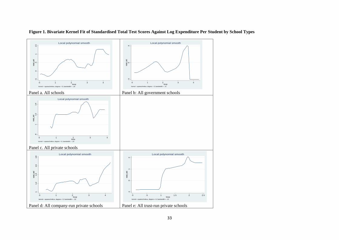
33  

Figure 1. Bivariate Kernel Fit of Standardised Total Test Scores Against Log Expenditure Per Student by School Types

Panel a. All schools

Panel b: All government schools

Panel c. All private schools

Panel d: All company-run private schools

Panel e: All trust-run private schools

-.50

.51

1.5

tota

l_st

d

0 1 2 3 4lexp

kernel = epanechnikov, degree = 0, bandwidth = .18

Local polynomial smooth

-.50

.5to

tal_

std

0 1 2 3 4lexp

kernel = epanechnikov, degree = 0, bandwidth = .31

Local polynomial smooth

.81

1.2

1.4

tota

l_st

d

0 1 2 3 4lexp

kernel = epanechnikov, degree = 0, bandwidth = .33

Local polynomial smooth

11.

21.

41.

61.

8to

tal_

std

0 1 2 3 4lexp

kernel = epanechnikov, degree = 0, bandwidth = .32

Local polynomial smooth

-10

12

tota

l_st

d

0 .5 1 1.5 2 2.5lexp

kernel = epanechnikov, degree = 0, bandwidth = .21

Local polynomial smooth

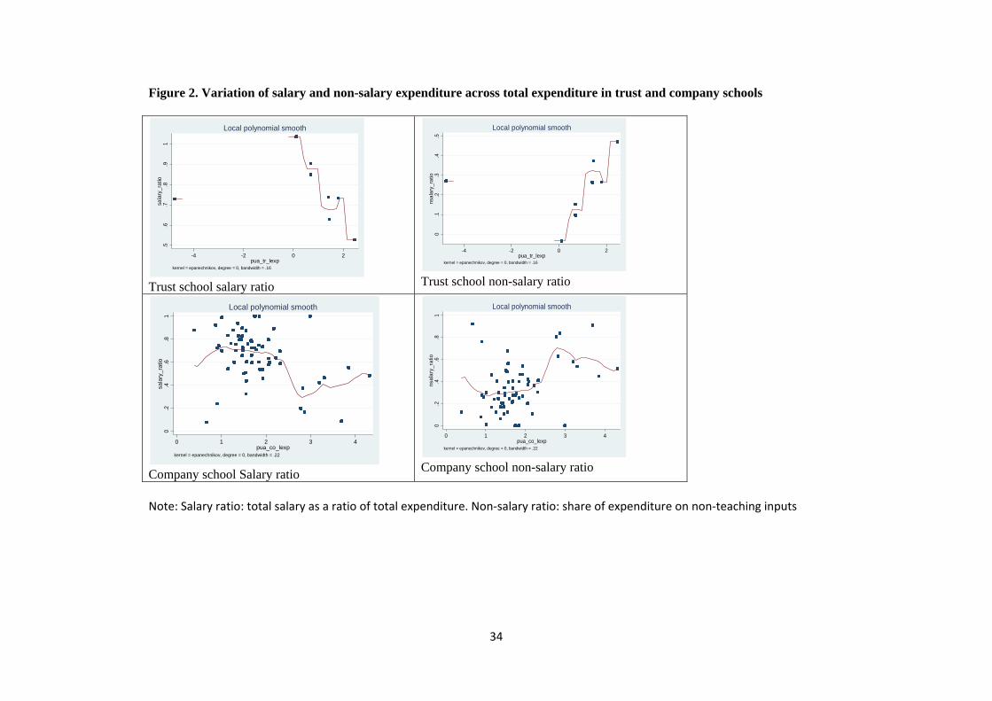
34  

Figure 2. Variation of salary and non-salary expenditure across total expenditure in trust and company schools  

Trust school salary ratio

Trust school non-salary ratio

Company school Salary ratio

Company school non-salary ratio

 Note: Salary ratio: total salary as a ratio of total expenditure. Non‐salary ratio: share of expenditure on non‐teaching inputs 

 

   

.5.6

.7.8

.91

sala

ry_r

atio

-4 -2 0 2pua_tr_lexp

kernel = epanechnikov, degree = 0, bandwidth = .16

Local polynomial smooth

0.1

.2.3

.4.5

nsal

ary_

ratio

-4 -2 0 2pua_tr_lexp

kernel = epanechnikov, degree = 0, bandwidth = .16

Local polynomial smooth

0.2

.4.6

.81

sala

ry_r

atio

0 1 2 3 4pua_co_lexp

kernel = epanechnikov, degree = 0, bandwidth = .22

Local polynomial smooth

0.2

.4.6

.81

nsal

ary_

ratio

0 1 2 3 4pua_co_lexp

kernel = epanechnikov, degree = 0, bandwidth = .22

Local polynomial smooth

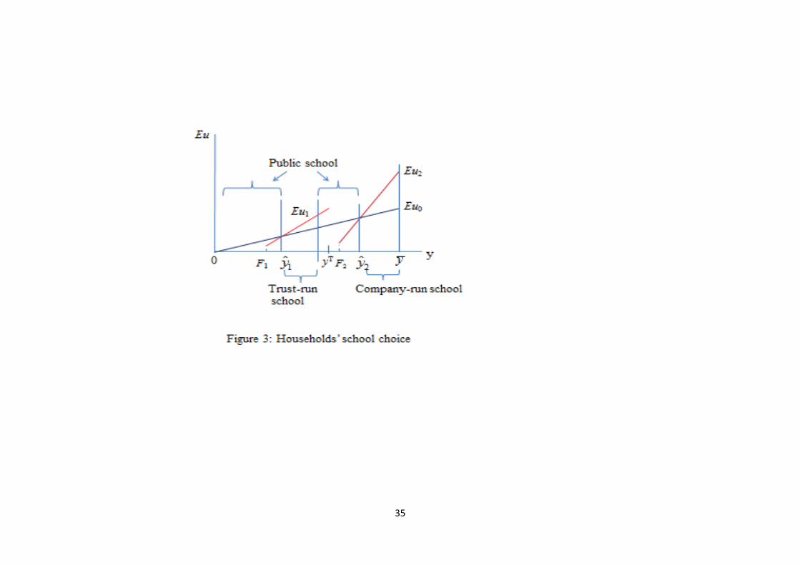
35  

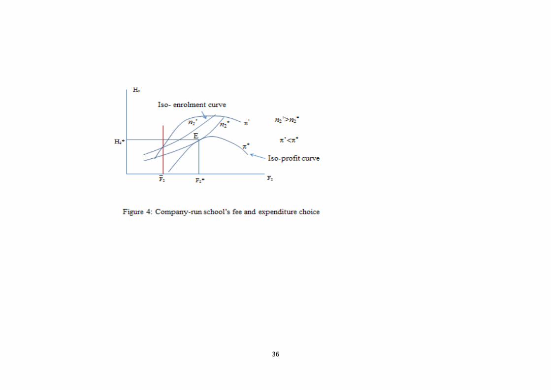
36  

 

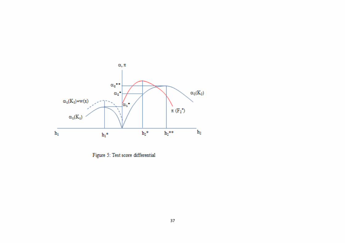
37  

 

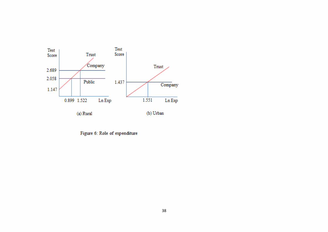
38  

 

   

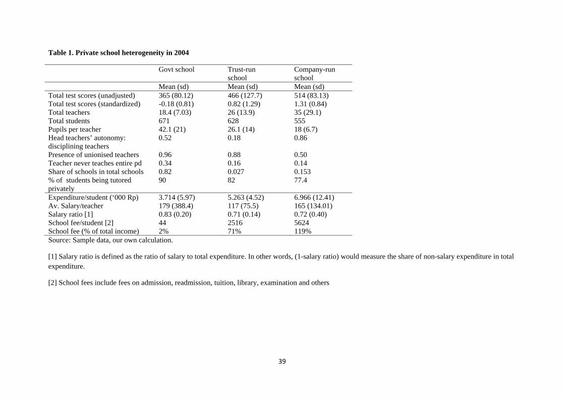
39  

Table 1. Private school heterogeneity in 2004

Govt school Trust-run school

Company-run school

Mean (sd) Mean (sd) Mean (sd) Total test scores (unadjusted) 365 (80.12) 466 (127.7) 514 (83.13) Total test scores (standardized) -0.18 (0.81) 0.82 (1.29) 1.31 (0.84) Total teachers 18.4 (7.03) 26 (13.9) 35 (29.1) Total students 671 628 555 Pupils per teacher 42.1 (21) 26.1 (14) 18 (6.7) Head teachers’ autonomy: disciplining teachers

0.52 0.18 0.86

Presence of unionised teachers 0.96 0.88 0.50 Teacher never teaches entire pd 0.34 0.16 0.14 Share of schools in total schools 0.82 0.027 0.153 % of students being tutored privately

90 82 77.4

Expenditure/student (‘000 Rp) 3.714 (5.97) 5.263 (4.52) 6.966 (12.41) Av. Salary/teacher 179 (388.4) 117 (75.5) 165 (134.01) Salary ratio [1] 0.83 (0.20) 0.71 (0.14) 0.72 (0.40) School fee/student [2] 44 2516 5624 School fee (% of total income) 2% 71% 119% Source: Sample data, our own calculation.

[1] Salary ratio is defined as the ratio of salary to total expenditure. In other words, (1-salary ratio) would measure the share of non-salary expenditure in total expenditure.

[2] School fees include fees on admission, readmission, tuition, library, examination and others

 

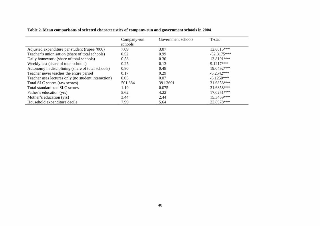
40  

Table 2. Mean comparisons of selected characteristics of company-run and government schools in 2004

Company-run schools

Government schools T-stat

Adjusted expenditure per student (rupee ‘000) 7.09 3.87 12.8015*** Teacher’s unionisation (share of total schools) 0.52 0.99 -52.3175*** Daily homework (share of total schools) 0.53 0.30 13.8191*** Weekly test (share of total schools) 0.25 0.13 9.1217*** Autonomy in disciplining (share of total schools) 0.80 0.48 19.0492*** Teacher never teaches the entire period 0.17 0.29 -6.2542*** Teacher uses lectures only (no student interaction) 0.05 0.07 -6.1250*** Total SLC scores (raw scores) 501.384 391.3691 31.6858*** Total standardized SLC scores 1.19 0.075 31.6858*** Father’s education (yrs) 5.62 4.22 17.0251*** Mother’s education (yrs) 3.44 2.44 15.3469*** Household expenditure decile 7.99 5.64 23.8978***

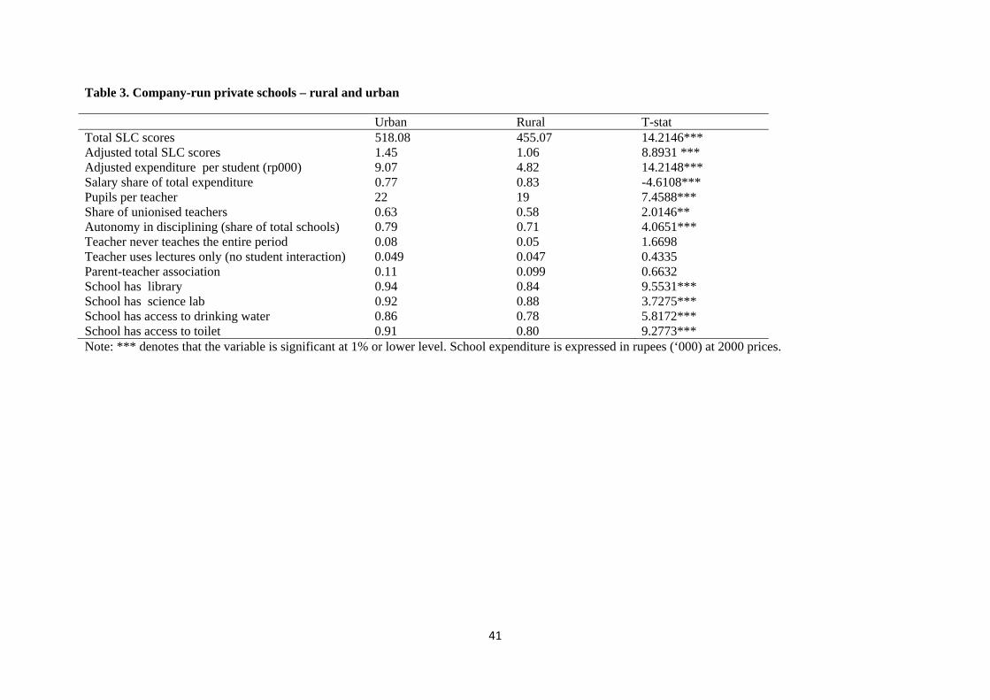
41  

Table 3. Company-run private schools – rural and urban

Urban Rural T-stat Total SLC scores 518.08 455.07 14.2146*** Adjusted total SLC scores 1.45 1.06 8.8931 *** Adjusted expenditure per student (rp000) 9.07 4.82 14.2148*** Salary share of total expenditure 0.77 0.83 -4.6108*** Pupils per teacher 22 19 7.4588*** Share of unionised teachers 0.63 0.58 2.0146** Autonomy in disciplining (share of total schools) 0.79 0.71 4.0651*** Teacher never teaches the entire period 0.08 0.05 1.6698 Teacher uses lectures only (no student interaction) 0.049 0.047 0.4335 Parent-teacher association 0.11 0.099 0.6632 School has library 0.94 0.84 9.5531*** School has science lab 0.92 0.88 3.7275*** School has access to drinking water 0.86 0.78 5.8172*** School has access to toilet 0.91 0.80 9.2773*** Note: *** denotes that the variable is significant at 1% or lower level. School expenditure is expressed in rupees (‘000) at 2000 prices.

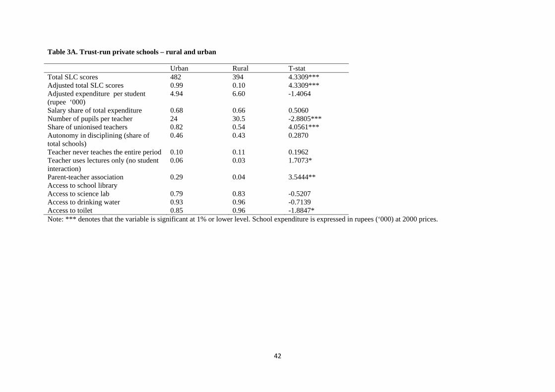
42  

Table 3A. Trust-run private schools – rural and urban

Urban Rural T-stat Total SLC scores 482 394 4.3309*** Adjusted total SLC scores 0.99 0.10 4.3309*** Adjusted expenditure per student (rupee ‘000)

4.94 6.60 -1.4064

Salary share of total expenditure 0.68 0.66 0.5060 Number of pupils per teacher 24 30.5 -2.8805*** Share of unionised teachers 0.82 0.54 4.0561*** Autonomy in disciplining (share of total schools)

0.46 0.43 0.2870

Teacher never teaches the entire period 0.10 0.11 0.1962 Teacher uses lectures only (no student interaction)

0.06 0.03 1.7073*

Parent-teacher association 0.29 0.04 3.5444** Access to school library Access to science lab 0.79 0.83 -0.5207 Access to drinking water 0.93 0.96 -0.7139 Access to toilet 0.85 0.96 -1.8847* Note: *** denotes that the variable is significant at 1% or lower level. School expenditure is expressed in rupees (‘000) at 2000 prices.

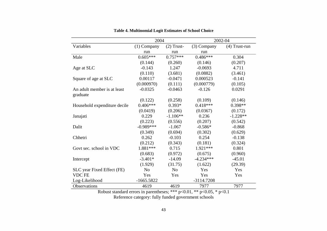
43  

Table 4. Multinomial Logit Estimates of School Choice

2004 2002-04 Variables (1) Company

run (2) Trust-

run (3) Company

run (4) Trust-run

Male 0.605*** 0.757*** 0.486*** 0.304 (0.144) (0.260) (0.146) (0.207) Age at SLC -0.143 1.247 -0.0693 4.711 (0.110) (3.681) (0.0882) (3.461) Square of age at SLC 0.00117 -0.0471 0.000523 -0.141 (0.000970) (0.111) (0.000779) (0.105) An adult member is at least graduate

-0.0325 -0.0463 -0.126 0.0291

(0.122) (0.258) (0.109) (0.146) Household expenditure decile 0.406*** 0.393* 0.418*** 0.398** (0.0419) (0.206) (0.0367) (0.172) Janajati 0.229 -1.106** 0.236 -1.228** (0.223) (0.556) (0.207) (0.542) Dalit -0.989*** -1.067 -0.586* -0.868 (0.349) (0.694) (0.302) (0.629) Chhetri 0.262 -0.103 0.254 -0.138 (0.212) (0.343) (0.181) (0.324) Govt sec. school in VDC 1.881*** 0.715 1.921*** 0.801 (0.683) (0.972) (0.675) (0.960) Intercept -3.401* -14.09 -4.234*** -45.01 (1.929) (31.75) (1.622) (29.39) SLC year Fixed Effect (FE) No No Yes Yes VDC FE Yes Yes Yes Yes Log-Likelihood -1665.5822 -3114.7208 Observations 4619 4619 7977 7977

Robust standard errors in parentheses; *** p<0.01, ** p<0.05, * p<0.1 Reference category: fully funded government schools

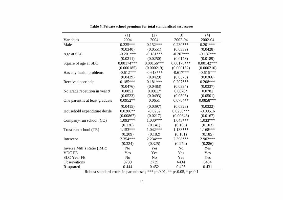
44  

Table 5. Private school premium for total standardised test scores

(1) (2) (3) (4) Variables 2004 2004 2002-04 2002-04 Male 0.225*** 0.152*** 0.230*** 0.201*** (0.0340) (0.0551) (0.0339) (0.0428) Age at SLC -0.201*** -0.181*** -0.207*** -0.187*** (0.0211) (0.0250) (0.0173) (0.0189) Square of age at SLC 0.00174*** 0.00156*** 0.00178*** 0.00142*** (0.000185) (0.000219) (0.000152) (0.000210) Has any health problems -0.612*** -0.613*** -0.617*** -0.616*** (0.0439) (0.0429) (0.0370) (0.0366) Received peer help 0.185*** 0.181*** 0.207*** 0.208*** (0.0476) (0.0483) (0.0334) (0.0337) No grade repetition in year 9 0.0851 0.0911* 0.0878* 0.0781   (0.0523) (0.0493) (0.0506) (0.0501) One parent is at least graduate  0.0952** 0.0651 0.0784** 0.0858*** (0.0415) (0.0397) (0.0328) (0.0322) Household expenditure decile 0.0206** -0.0252 0.0256*** -0.00516 (0.00867) (0.0217) (0.00646) (0.0167) Company-run school (CO) 1.093*** 1.030*** 1.043*** 1.033*** (0.136) (0.141) (0.105) (0.103) Trust-run school (TR) 1.153*** 1.042*** 1.133*** 1.168*** (0.209) (0.182) (0.181) (0.185) Intercept 2.354*** 2.234*** 2.398*** 2.902*** (0.324) (0.325) (0.279) (0.286) Inverse Mill’s Ratio (IMR) No Yes No Yes VDC FE Yes Yes Yes Yes SLC Year FE No No Yes Yes Observations 3739 3739 6434 6434 R-squared 0.444 0.452 0.425 0.431

Robust standard errors in parentheses; *** p<0.01, ** p<0.05, * p<0.1

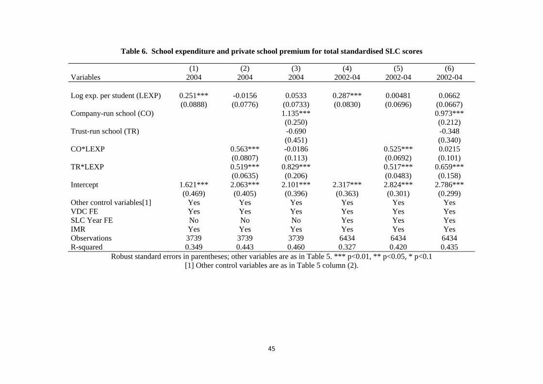
45  

Table 6. School expenditure and private school premium for total standardised SLC scores

(1) (2) (3) (4) (5) (6) Variables 2004 2004 2004 2002-04 2002-04 2002-04 Log exp. per student (LEXP) 0.251*** -0.0156 0.0533 0.287*** 0.00481 0.0662 (0.0888) (0.0776) (0.0733) (0.0830) (0.0696) (0.0667) Company-run school (CO) 1.135*** 0.973*** (0.250) (0.212) Trust-run school (TR) -0.690 -0.348 (0.451) (0.340) CO*LEXP 0.563*** -0.0186 0.525*** 0.0215 (0.0807) (0.113) (0.0692) (0.101) TR*LEXP 0.519*** 0.829*** 0.517*** 0.659*** (0.0635) (0.206) (0.0483) (0.158) Intercept 1.621*** 2.063*** 2.101*** 2.317*** 2.824*** 2.786*** (0.469) (0.405) (0.396) (0.363) (0.301) (0.299) Other control variables[1] Yes Yes Yes Yes Yes Yes VDC FE Yes Yes Yes Yes Yes Yes SLC Year FE No No No Yes Yes Yes IMR Yes Yes Yes Yes Yes Yes Observations 3739 3739 3739 6434 6434 6434 R-squared 0.349 0.443 0.460 0.327 0.420 0.435

Robust standard errors in parentheses; other variables are as in Table 5. *** p<0.01, ** p<0.05, * p<0.1 [1] Other control variables are as in Table 5 column (2).

46  

Table 6A. Total standardised test score estimates with control for low/high fee company schools

(1) (2) Variables 2004 2002-04 Log exp. per student (LEXP) -0.0979 -0.0702 (0.0659) (0.0550) Trust-run school (TR) -0.148 -0.0381 (0.604) (0.495) High fee CO school 1.164*** 1.011*** (0.284) (0.228) Low fee CO school 0.252 0.175 (0.468) (0.325) TR*LEXP 0.699*** 0.604*** (0.257) (0.213) High fee CO school*LEXP 0.0408 0.0757 (0.120) (0.101) Low fee CO school*LEXP 0.355 0.395** (0.246) (0.161) Constant 2.413*** 2.411*** (0.327) (0.276) Other control variables Yes Yes VDC FE Yes Yes SLC year FE No Yes IMR Yes Yes Observations 4,586 7,894 R-squared 0.429 0.412

Robust standard errors are in parentheses; *** p<0.01, ** p<0.05, * p<0.1. Other control variables are as in Table 5.

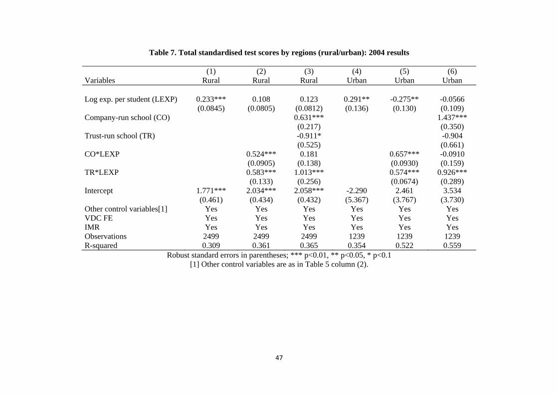
47  

Table 7. Total standardised test scores by regions (rural/urban): 2004 results

(1) (2) (3) (4) (5) (6) Variables Rural Rural Rural Urban Urban Urban Log exp. per student (LEXP) 0.233*** 0.108 0.123 0.291** -0.275** -0.0566 (0.0845) (0.0805) (0.0812) (0.136) (0.130) (0.109) Company-run school (CO) 0.631*** 1.437*** (0.217) (0.350) Trust-run school (TR) -0.911* -0.904 (0.525) (0.661) CO*LEXP 0.524*** 0.181 0.657*** -0.0910 (0.0905) (0.138) (0.0930) (0.159) TR*LEXP 0.583*** 1.013*** 0.574*** 0.926*** (0.133) (0.256) (0.0674) (0.289) Intercept 1.771*** 2.034*** 2.058*** -2.290 2.461 3.534 (0.461) (0.434) (0.432) (5.367) (3.767) (3.730) Other control variables[1] Yes Yes Yes Yes Yes Yes VDC FE Yes Yes Yes Yes Yes Yes IMR Yes Yes Yes Yes Yes Yes Observations 2499 2499 2499 1239 1239 1239 R-squared 0.309 0.361 0.365 0.354 0.522 0.559

Robust standard errors in parentheses; *** p<0.01, ** p<0.05, * p<0.1 [1] Other control variables are as in Table 5 column (2).

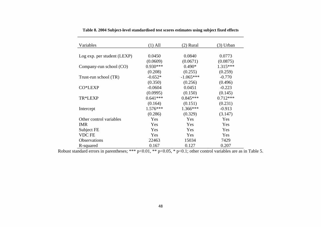
48  

Table 8. 2004 Subject-level standardised test scores estimates using subject fixed effects

Variables (1) All (2) Rural (3) Urban Log exp. per student (LEXP) 0.0450 0.0840 0.0773 (0.0609) (0.0671) (0.0875) Company-run school (CO) 0.930*** 0.490* 1.315*** (0.208) (0.255) (0.259) Trust-run school (TR) -0.652* -1.065*** -0.770 (0.350) (0.256) (0.496) CO*LEXP -0.0604 0.0451 -0.223 (0.0995) (0.150) (0.145) TR*LEXP 0.641*** 0.845*** 0.712*** (0.164) (0.151) (0.231) Intercept 1.576*** 1.366*** -0.913 (0.286) (0.329) (3.147) Other control variables Yes Yes Yes IMR Yes Yes Yes Subject FE Yes Yes Yes VDC FE Yes Yes Yes Observations 22463 15034 7429 R-squared 0.167 0.127 0.207

Robust standard errors in parentheses; *** p<0.01, ** p<0.05, * p<0.1; other control variables are as in Table 5.

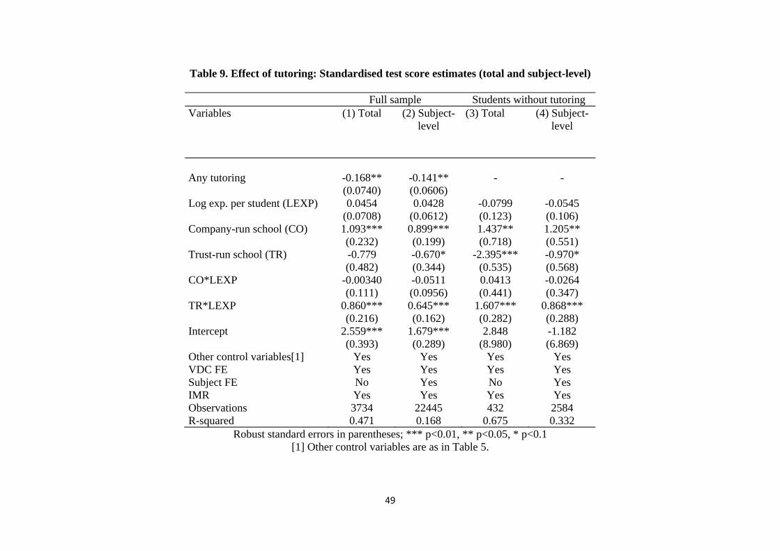
49  

Table 9. Effect of tutoring: Standardised test score estimates (total and subject-level)

Full sample Students without tutoring Variables (1) Total

(2) Subject-

level

(3) Total (4) Subject-level

Any tutoring -0.168** -0.141** - - (0.0740) (0.0606) Log exp. per student (LEXP) 0.0454 0.0428 -0.0799 -0.0545 (0.0708) (0.0612) (0.123) (0.106) Company-run school (CO) 1.093*** 0.899*** 1.437** 1.205** (0.232) (0.199) (0.718) (0.551) Trust-run school (TR) -0.779 -0.670* -2.395*** -0.970* (0.482) (0.344) (0.535) (0.568) CO*LEXP -0.00340 -0.0511 0.0413 -0.0264 (0.111) (0.0956) (0.441) (0.347) TR*LEXP 0.860*** 0.645*** 1.607*** 0.868*** (0.216) (0.162) (0.282) (0.288) Intercept 2.559*** 1.679*** 2.848 -1.182 (0.393) (0.289) (8.980) (6.869) Other control variables[1] Yes Yes Yes Yes VDC FE Yes Yes Yes Yes Subject FE No Yes No Yes IMR Yes Yes Yes Yes Observations 3734 22445 432 2584 R-squared 0.471 0.168 0.675 0.332

Robust standard errors in parentheses; *** p<0.01, ** p<0.05, * p<0.1 [1] Other control variables are as in Table 5.

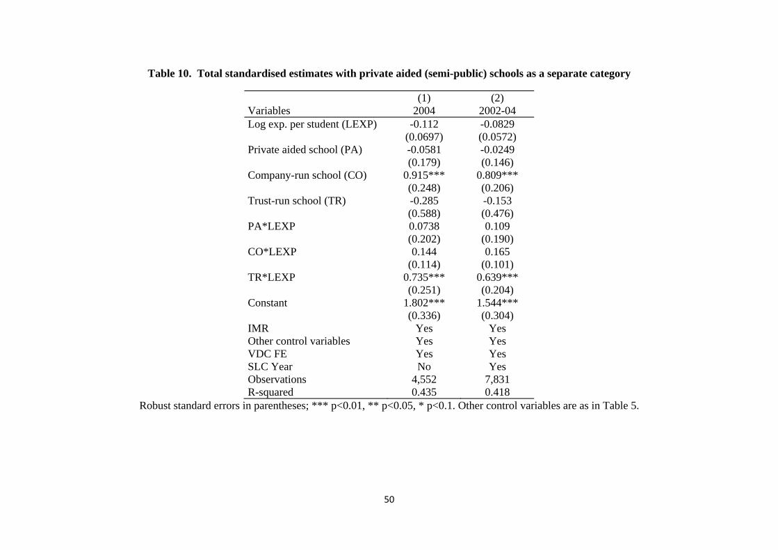
50  

Table 10. Total standardised estimates with private aided (semi-public) schools as a separate category

(1) (2) Variables 2004 2002-04 Log exp. per student (LEXP) -0.112 -0.0829 (0.0697) (0.0572) Private aided school (PA) -0.0581 -0.0249 (0.179) (0.146) Company-run school (CO) 0.915*** 0.809*** (0.248) (0.206) Trust-run school (TR) -0.285 -0.153 (0.588) (0.476) PA*LEXP 0.0738 0.109 (0.202) (0.190) CO*LEXP 0.144 0.165 (0.114) (0.101) TR*LEXP 0.735*** 0.639*** (0.251) (0.204) Constant 1.802*** 1.544*** (0.336) (0.304) IMR Yes Yes Other control variables Yes Yes VDC FE Yes Yes SLC Year No Yes Observations 4,552 7,831 R-squared 0.435 0.418

Robust standard errors in parentheses; *** p<0.01, ** p<0.05, * p<0.1. Other control variables are as in Table 5.

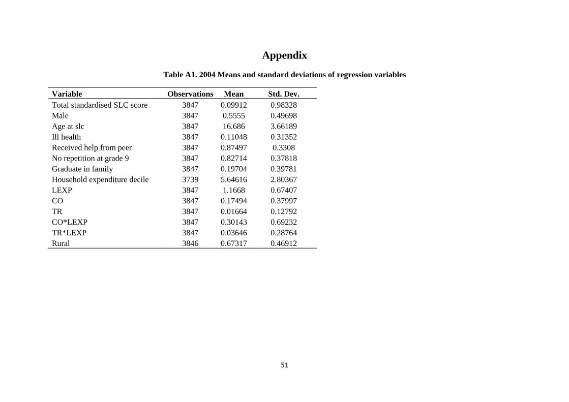
51  

Appendix

Table A1. 2004 Means and standard deviations of regression variables

Variable Observations Mean Std. Dev. Total standardised SLC score 3847 0.09912 0.98328 Male 3847 0.5555 0.49698 Age at slc 3847 16.686 3.66189 Ill health 3847 0.11048 0.31352 Received help from peer 3847 0.87497 0.3308 No repetition at grade 9 3847 0.82714 0.37818 Graduate in family 3847 0.19704 0.39781 Household expenditure decile 3739 5.64616 2.80367 LEXP 3847 1.1668 0.67407 CO 3847 0.17494 0.37997 TR 3847 0.01664 0.12792 CO*LEXP 3847 0.30143 0.69232 TR*LEXP 3847 0.03646 0.28764 Rural 3846 0.67317 0.46912

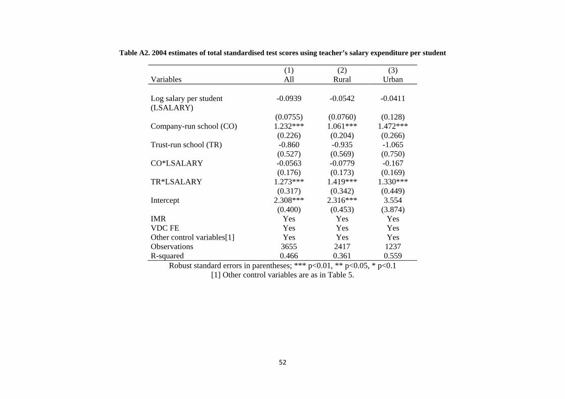
52  

Table A2. 2004 estimates of total standardised test scores using teacher’s salary expenditure per student

(1) (2) (3) Variables All Rural Urban Log salary per student (LSALARY)

-0.0939 -0.0542 -0.0411

(0.0755) (0.0760) (0.128) Company-run school (CO) 1.232*** 1.061*** 1.472*** (0.226) (0.204) (0.266) Trust-run school (TR) -0.860 -0.935 -1.065 (0.527) (0.569) (0.750) CO*LSALARY -0.0563 -0.0779 -0.167 (0.176) (0.173) (0.169) TR*LSALARY 1.273*** 1.419*** 1.330*** (0.317) (0.342) (0.449) Intercept 2.308*** 2.316*** 3.554 (0.400) (0.453) (3.874) IMR Yes Yes Yes VDC FE Yes Yes Yes Other control variables[1] Yes Yes Yes Observations 3655 2417 1237 R-squared 0.466 0.361 0.559

Robust standard errors in parentheses; *** p<0.01, ** p<0.05, * p<0.1 [1] Other control variables are as in Table 5.

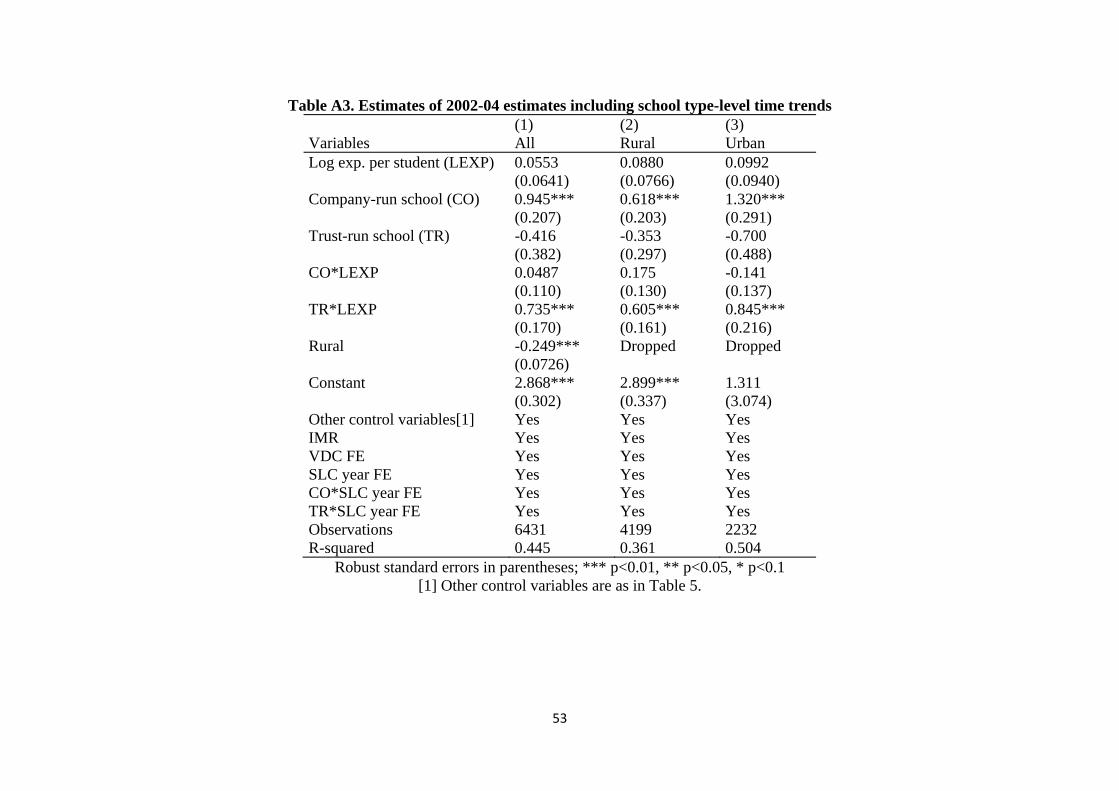
53  

Table A3. Estimates of 2002-04 estimates including school type-level time trends (1) (2) (3) Variables All Rural Urban Log exp. per student (LEXP) 0.0553 0.0880 0.0992 (0.0641) (0.0766) (0.0940) Company-run school (CO) 0.945*** 0.618*** 1.320*** (0.207) (0.203) (0.291) Trust-run school (TR) -0.416 -0.353 -0.700 (0.382) (0.297) (0.488) CO*LEXP 0.0487 0.175 -0.141 (0.110) (0.130) (0.137) TR*LEXP 0.735*** 0.605*** 0.845*** (0.170) (0.161) (0.216) Rural -0.249*** Dropped Dropped (0.0726) Constant 2.868*** 2.899*** 1.311 (0.302) (0.337) (3.074) Other control variables[1] Yes Yes Yes IMR Yes Yes Yes VDC FE Yes Yes Yes SLC year FE Yes Yes Yes CO*SLC year FE Yes Yes Yes TR*SLC year FE Yes Yes Yes Observations 6431 4199 2232 R-squared 0.445 0.361 0.504

Robust standard errors in parentheses; *** p<0.01, ** p<0.05, * p<0.1 [1] Other control variables are as in Table 5.

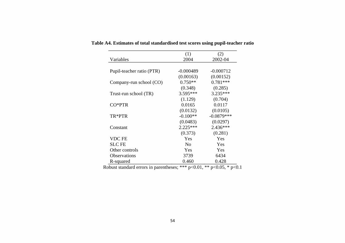
54  

Table A4. Estimates of total standardised test scores using pupil-teacher ratio

(1) (2) Variables 2004 2002-04 Pupil-teacher ratio (PTR) -0.000489 -0.000712 (0.00163) (0.00152) Company-run school (CO) 0.750** 0.781*** (0.348) (0.285) Trust-run school (TR) 3.595*** 3.235*** (1.129) (0.704) CO*PTR 0.0165 0.0117 (0.0132) (0.0105) TR*PTR -0.100** -0.0879*** (0.0483) (0.0297) Constant 2.225*** 2.436*** (0.373) (0.281) VDC FE Yes Yes SLC FE No Yes Other controls Yes Yes Observations 3739 6434 R-squared 0.460 0.428

Robust standard errors in parentheses; *** p<0.01, ** p<0.05, * p<0.1

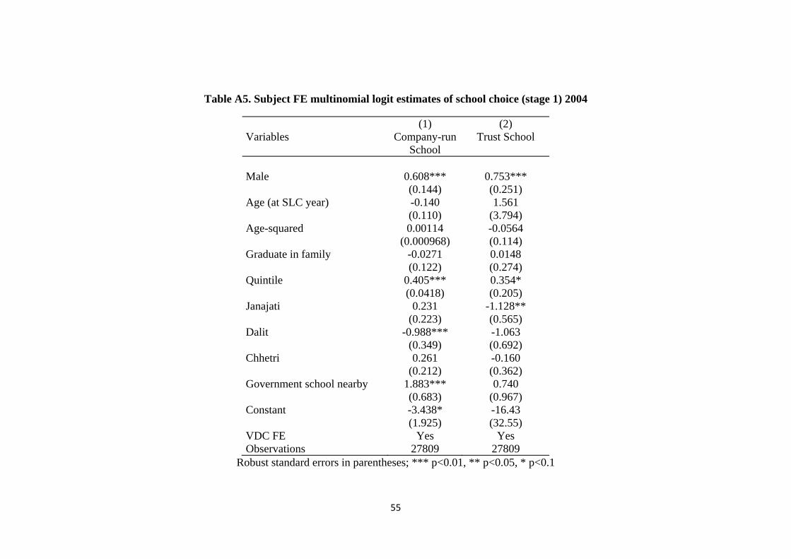
55  

Table A5. Subject FE multinomial logit estimates of school choice (stage 1) 2004

(1) (2) Variables Company-run

School Trust School

Male 0.608*** 0.753*** (0.144) (0.251) Age (at SLC year) -0.140 1.561 (0.110) (3.794) Age-squared 0.00114 -0.0564 (0.000968) (0.114) Graduate in family -0.0271 0.0148 (0.122) (0.274) Quintile 0.405*** 0.354* (0.0418) (0.205) Janajati 0.231 -1.128** (0.223) (0.565) Dalit -0.988*** -1.063 (0.349) (0.692) Chhetri 0.261 -0.160 (0.212) (0.362) Government school nearby 1.883*** 0.740 (0.683) (0.967) Constant -3.438* -16.43 (1.925) (32.55) VDC FE Yes Yes Observations 27809 27809

Robust standard errors in parentheses; *** p<0.01, ** p<0.05, * p<0.1    

56  

Table A6. Multinomial logit estimates of school choice including private aided (PA) schools

2002-04 2004 (1) (2) (3) (4) (5) (6) Variables PA Trust Company-run PA Trust Company-run Male -0.197* 0.188 0.503*** -0.318** 0.489* 0.646*** (0.100) (0.195) (0.139) (0.127) (0.289) (0.142) Age (at SLC year) 0.0833 3.652** -0.0648 0.0473 0.949 -0.128 (0.0647) (1.536) (0.0871) (0.0832) (1.471) (0.109) Age-squared -0.000860 -0.105** 0.000493 -0.000526 -0.0290 0.00104 (0.000590) (0.0474) (0.000768) (0.000738) (0.0438) (0.000955) Graduate in family -0.0247 0.185 -0.0872 0.00428 0.157 0.00324 (0.110) (0.114) (0.105) (0.132) (0.193) (0.116) Quintile -0.100** 0.286** 0.420*** -0.107** 0.252 0.404*** (0.0411) (0.142) (0.0367) (0.0454) (0.157) (0.0417) Janajati 0.389* -0.503 0.318 0.448* -0.457 0.304 (0.208) (0.372) (0.201) (0.236) (0.399) (0.222) Dalit -0.201 -0.722 -0.518* -0.0750 -0.744 -0.937*** (0.197) (0.646) (0.299) (0.216) (0.681) (0.348) Chhetri 0.104 -0.365 0.238 0.156 -0.395 0.250 (0.179) (0.321) (0.179) (0.201) (0.386) (0.207) Government school nearby -0.736* -1.090 1.746*** -0.769** -1.159 1.728** (0.376) (0.950) (0.652) (0.392) (0.955) (0.682) Rural 0.167 -1.352** 0.0912 0.0363 -1.546** 0.0594 (0.344) (0.616) (0.341) (0.371) (0.642) (0.378) Constant -2.219** -34.77*** -4.209*** -1.436 -10.86 -3.560* (1.129) (13.07) (1.601) (1.346) (12.80) (1.929) VDC FE Yes Yes Yes Yes Yes Yes SLC Year FE Yes Yes Yes No No No Observations 9,666 9,666 9,666 5,612 5,612 5,612

Robust standard errors in parentheses; *** p<0.01, ** p<0.05, * p<0.1. The reference category is the government schools.