Corruption, Default and Optimal Credit in Welfare Programs

April 22, 2004

BIBHAS SAHA

Indira Gandhi Institute of Development Research, India

TRIVIKRAMAN THAMPY

New York University, USA

Address:

Bibhas Saha

Indira Gandhi Institute of Development Research

Gen. Vaidya Marg, Goregaon (E)

Mumbai 400065, INDIA

e-mails: bibhas@igidr.ac.in, tst214@nyu.edu

1

Abstract

In this paper we present a dynamic model of subsidized credit provision to examine

how asymmetric information exacerbates inefficiency caused by corruption. Though de-

signed to empower the underprivileged, the fate of such credit programs largely depends

on the efficiency of the credit delivery system. Corruption often erodes this efficiency.

Nevertheless, when a corrupt loan official and a borrower interact with symmetric infor-

mation, credit terms can be so designed that corruption will affect only the size of the

surplus, but not repayment. With private information on the borrower’s productivity

this result changes. The corrupt loan official may induce the low productivity borrower

to default, mainly because of high revelation costs. The government can improve the

repayment rate, but will have to under-provide the first period loan. On the other hand it

can permit default by the low productivity borrower, and maintain a higher credit level.

The second option may sometimes be preferred. This inefficient outcome is caused by two

factors - informational ratchet effects and countervailing incentives, which are commonly

present in many agency relationships.

Keywords: Corruption, Information rent, Countervailing incentives, Ratchet effect

JEL Classification: H2;D8;K4

Acknowledgements: We are grateful to two anonymous referees and an associate editor

of a journal for their valuable comments, which helped us substantially revise the paper. On

several earlier versions, we have received helpful comments from Arindam Dasgupta, Ashima

Goyal, Arye L. Hillman, Debraj Ray, and seminar participants at IGIDR, Mumbai and ISI,

Kolkata. This paper is partially based on one chapter of the second author’s M. Phil thesis

done at IGIDR. For any remaining errors we are solely responsible.

2

1 Introduction

Subsidized credit programs are quite common in developing countries. These may include pro-

viding cheap loans to farmers, special credit to small businesses, and subsidy to exporters and

so on so forth. But such programs suffer from two problems: high incidence of default (Hoff

and Stiglitz; 1990) and corruption in implementation (Rose-Ackerman, 1999).1 Economists

generally focus on the default problem and their explanations vary from adverse selections,

imperfect screening of borrowers, and incorrect design of credit contracts to wrong targeting.

Political economists, on the other hand, provide a great deal of evidence of corruption, and

their concern is often shared by aid agencies and practitioners.2 Thus, there can be an as-

sociation between corruption and default that may not be coincidental.3 Unfortunately, no

empirical and theoretical studies have examined the link between the two phenomena. The

present paper makes a theoretical attempt to do so with the help of a dynamic model of credit

provision.

In general, corruption in credit provision is common to a large number of countries.4 At

a micro level, various field studies in India report two types of corruption in the provision of

agricultural credit through government agencies. One type of corruption involves diverting

credit to the rich or locally powerful farmers. Such powerful borrowers are also believed to be

big defaulters (Sarap, 1991).5 The other type of corruption involves poor or not-so-powerful1Hoff and Stiglitz (1990) note that ‘high default rates have prevented (formal lending) institutions from

being self-financing’, and ‘despite these subsidies, many of these credit programs have had very little success

in reaching farmers without collateral or with below-average income.’ Thus, Hoff and Stiglitz emphasize on

two aspects: high default rates and designs or delivery of credit.2The World Bank (1997, p.59) noted that in South Asia in 1991-92 only 10 percent of public subsidies

reached the households below median income. In a similar vein, India’s former Prime Minister, the late Rajiv

Gandhi, once lamented that of every rupee that was spent for the poor, only 20 percent eventually reached

the target.3In Kenya, it was estimated that a third of banking assets in 1992 were rendered worthless because of

political interference and favoritism (Rose-Ackerman, 1999, p.10). In rural Pakistan, one field study conducted

in 1980-81, found 30 percent of loans from government operated banks were getting defaulted, while the same

rate for the local moneylender was only 2.7 percent (Hoff and Stiglitz, 1990).4Rose-Ackerman (1999, p.10) writes, “If the supply of credit and the rate of interest are controlled by the

state, bribes may be paid for access. Interviews with business people in Eastern Europe and Russia indicate

that payoffs are frequently needed to obtain credit... In Lebanon a similar survey revealed that loans were not

available without the payment of bribes.”5Sarap (1991) in his field study in some parts of Eastern India notes that local rich and politically powerful

3

farmers, who may be subjected to harassment by a corrupt official (Dreze, 1990; Balmohandas

et al, 1991; Jodhka, 1995).6 In the former case, the well-connected farmer is powerful enough

to capture the subsidy meant for others. In the latter, legitimate borrowers fall pray to

corrupt officials. Defaults in this case may be a result of the official’s extractiveness. Our

objective is to study the second scenario.

While the above studies are useful, very little can be ascertained from them about the link

between corruption and default. Given this lack of a pointed empirical study, a theoretical

investigation can provide some insight and also some direction of empirical research. Keeping

this objective in mind, we raise two questions: Why and when would a corrupt official like

to force a borrower to default, and if so, what would be the optimal credit scheme from the

government’s point of view? The first question is an issue of a positive analysis, as it may help

us speculate on the repayment performance of certain types of credit schemes in a corrupt

environment. The second question is important from the policy point of view. A number of

studies have emphasized on the adverse consequences of corruption on the provision of public

people (ranging from large farmers, teachers, and lawyers to traders) are treated on a preferential basis. This

group receives bulk of the subsidized credit. However, he found that delay was much more of a problem than

bribe, and delay was inversely related to the borrower’s wealth or social status (such as land-holding). He also

notes that 65 percent of the borrowers in his sample defaulted on their loans. At the national level, Reserve

Bank of India, reports that at 2000-01, compared to the small farmers, rich farmers received 1.90 times more

loans (in amounts) from the commercial banks, but the loans outstanding from them was 2.35 times greater

than that from the small farmers (Tables 52, 53, Reserve Bank of India, 2002-03). The Indian government

also admitted that in 1996 it failed to recover 40 percent of agricultural loans given by state-owned banks

(Government of India, 1998). Though these are aggregate figures, and loans can be of various types, we do get

a feel that the problem of default really endemic.6In the context of the rural economy of India, it has been observed that corruption varies in terms of

forms and intensities depending on the type of agencies that are in charge of delivering credit. While rural

branches of large commercial banks follow more standardized procedures that restrict corruption, localized

loan agencies can be a playground for bureaucrats, politicians and the local elite. Dreze (1990) observes that

poor farmers in a North Indian village had to pay some bribes to get a loan in connection with an anti-poverty

program. Another North Indian field study (Jodhka, 1995) shows how an all-powerful bureaucrat in charge

of a cooperative bank can demand bribes at every step. However, this picture varies between regions. In

Southern India, Balmohandas et al (1991) observes that bribery, though quite common, is not extractive to

lead to default. In their survey, 45 percent of the borrowers admitted paying ’speed money’ to the tune of

about 10 percent of the loan amount, but the repayment rate was 80 percent. However, inordinate delays

(averaging three months) were a serious problem faced by 40 percent of the borrowers.

4

services (Shliefer and Vishny, 1993), on investment in human capital (Ehrlich and Lui, 1999),

and on the provision of health care and education services (Gupta et al, 2001). In a similar

vein, we ask: Is it optimal for the government to reduce the provision of credit?

We consider a two-period model of credit provision under asymmetric information with

the possibility that the loan official can be corrupt. The credit scheme we consider provides

incentive to repay through promise of bigger loans in future, instead of demanding substantial

collaterals. If the official is corrupt, he will extract bribe and cause delay to reduce the bor-

rower’s profit, but may not necessarily wish to see the borrower default. Being less extractive

now, he can sustain a stream of bribes over time, and if the government appropriately sets

the loan amounts, repayment can be ensured even when the official is corrupt. Thus, we

first establish that corruption, though reducing the borrower’s income need not increase the

default rate.

However, this argument turns out to be valid only under full information. If the borrower

has private information on his productivity, a corrupt official will have to incur ‘revelation

costs’, when he tries to extort bribes. Should he wish to deal with the borrower over time

(i.e. by inducing repayment), he must concede dynamic information rent to one type of the

borrower. On the other hand, a short-term dealing (i.e. by inducing default) would allow him

to save on large revelation cost, and therefore, in some situations default may be preferred. By

modeling the interaction between the borrower and the official as a principal agent problem

(or as a monopoly price discrimination problem), we are able to associate repayment with a

‘long term contract’ and default with a ‘short term contract’. We show that the probability

of the official offering a short term contract instead of a long term contract to certain types

of borrower - an inefficient outcome - is always positive, and cannot be driven to zero, unless

corruption is altogether eliminated.

We then ask: what would be the optimal credit scheme for the government? If it wishes

to restrict extraction and ensure repayment, it must reduce the size of the first period loan

to curb the corrupt official’s short-term payoff. A big wedge between the credit amounts of

the two periods seems necessary to align the long-term interest of the corrupt official with

that of the borrower. Thus, it may be optimal to under-provide credit in the current period,

if repayment is to be ensured. In some situations, however, the government can do better by

permitting default by certain type of borrowers, and can ease the under-provisioning problem.

5

Our approach broadly follows the well-established literature on misgovernance (Shleifer

and Vishny, 1993; Banerjee, 1997; Choi and Thum, 2003). While Shleifer and Vishny (1993)

and Banerjee (1997) offered static analysis of bureaucratic corruption, Choi and Thum (2003)

developed a dynamic version of Shleifer and Vishny. The possibility that a corrupt official

may repeat extortion in future distorts entry decisions of the entrepreneurs in the current

period. The official’s inability to commit to a future strategy reduces his monopoly power

and his bribes from selling permits. The ratchet effect causes inefficient entry decisions. In

our dynamic model also the informational ratchet effect reduces the long-term payoff of the

corrupt official and induces him to prefer default, - a short-term transaction. In addition, we

also observe that the default strategy is sometimes characterized by countervailing incentives,

which typically reduce the revelation costs, and make default a more attractive option. We

note that as long as one of these two factors is present, a model of our kind will make the

official’s behavior inefficient in the sense that he would induce default.

There are several other papers that have considered bribery, red tape or harassment. Lui

(1985) is one of the early contributions on queuing and bribery. Although we do not have

queues, red tape has some similarity with queuing. Chaudhuri and Gupta (1996) considered

a similar set up like ours in their analysis of bribery in the provision of formal credit, but their

main interest is to study the interaction between formal and informal credit markets. Default

is not an issue there. Saha (2001) has studied corruption in the provision of subsidy using

bribe and red tape as a screening device. This approach is similar to Banerjee (1997), and

is applied in this paper as well. In the present paper they are also indicators of harassment.

However, harassment or extortion can be modeled in different ways. See Hindriks et al (1999),

Marjit et al (2000) and Saha (2003) for different approaches to harassment in tax evasion.

But these papers share features of law enforcement models (Mishra, 2002), and do not pertain

to bureaucratic corruption, which is the main concern of this article.

The rest of the paper is organized as follows. In the next section we begin with the

benchmark case of full information where the official also observes the borrower’s productivity.

Then we move on to the asymmetric information case in Section 3, to consider the corrupt

official’s behavior when all types of borrowers are productive and then derive one of our main

results concerning default. In Section 4, we repeat the same exercise assuming that one type

of the borrower can be unproductive. Section 5 presents a discussion of what the government’s

6

optimal credit program should be. The concluding section discusses limitations of our work

and comments on some empirical issues

2 The model preliminaries

2.1 The setup

Our model has two periods and two players : one loan disbursing official (principal) and a

representative borrower (agent). There is also a third player, the higher authority (or simply

the government), who acts like a super-principal. In the first part of our analysis, the role of

the super-principal will be taken as exogenous; later we endogenize his decisions as well. The

borrower belongs to a population, which by a random draw of Nature contains p proportion of

high productivity (kh) individuals, and (1−p) proportion of low productivity (kl) individuals.7

A high productivity individual can always convert one dollar into a sum of more than one

dollar, but a low productivity individual may or may not be able to do so. This is captured

through the assumption that kh can take only one value, kH , which is greater than 1. On the

other hand, kl can take two values: kL and kU , kU < 1 < kL < kH . When kU is realized, the

individual becomes unproductive, and will invariably default on any loan he takes. Given that

a borrower’s productivity is not kH (or simply H type), he will be L type with probability β

and U type with probability (1−β). All low productivity borrowers are assumed to have the

same realization of kL.

The information structure: The government would like to advance the loan only to the

H or L types. But, neither it nor the loan official can distinguish borrower types, as the

realizations of kh and kl are only privately observed by the borrowers alone. Therefore,

unless the U type borrowers are discouraged through a high collateral or ex post penalty, it

is impossible to separate them from productive borrowers.

We reduce the informational uncertainty on the part of the official by assuming that he

learns whether the realization of kl has been kL or kU , but still he cannot distinguish H from

L or H from U . The official may have expertise (such as to conduct a market survey, or

process a public signal) to learn whether he is going to deal with a (kH , kL) distribution, or

a (kH , kU ) distribution, but cannot acquire finer information about individual borrowers.7Nothing is lost if the population size is set to be 1.

7

The terms of the loan: The borrower, whose loan has already been approved by the

higher authority by some mechanism, is to receive a loan of c1 dollars in the first period, and

c2 dollars in the second period, subject to the repayment of the first loan.8 The loan is interest

free, but carries a penalty on default. We permit quite a general structure of penalties: D1

on the default of c1 and D2 on c2. Although we are going to emphasize on an increasing

profile of penalties, D1 ≤ D2, no a priori restrictions are needed other than 0 ≤ D1 ≤ c1 and

0 ≤ D2 ≤ c2. These penalties can be interpreted in many ways. The simplest case is that

of collaterals. Another possibility is ex post fines, such as confiscation of household assets, or

temporary withdrawal of food subsidy or health benefits etc. In the extreme case, where the

borrower has no wealth whatsoever, D1 and D2 both can be zero.9

Anti-corruption measures: The efficiency of the loan delivery system depends on the

honesty of the loan-disbursing official. The government knows that the official will be honest

with probability q, and corruptible with probability (1− q). The official’s type is his private

information. An honest official never takes bribe and never delays delivering the loan. But a

corrupt official acts like a price-discriminating monopolist, who demands bribes and imposes

red tape for each type. The red tape here simply taken as unrecorded delay, from which the

official is assumed to derive utility. This means that though the loan is delivered at a later

date, the official record will carry no evidence of it.10 We must also add that such extortions8We do not go into the questions of how to screen credit-worthiness of the borrowers. The government can

ask the official to report their learning about kl, and may use that information while approving the loan. For

example, if the report is that kl = kU , a loan application may be approved only with probability p. Very often

eligibility for subsidized loans is centrally determined based on more observable criteria. But these issues are

not important for our formulation.9Many micro finance organizations in their dealings with poor borrowers, retain a part of their loans as a

proxy collateral, which is released only after some installments of the loan are repaid. Effectively, the loan

structure becomes dynamic. We should also note that our main concern for default is only about the first

period. The last period default problem can be eliminated by setting D2 as high as c2, and setting D2 high

may be feasible. After all, the credit subsidies offered in earlier periods could create wealth against which

future loans may be issued.10That the official derives positive utility from red tape is not essential. Red tape can be a pure waste as in

Banerjee (1997), for instance. However, in developing countries where government employees are often poorly

paid, their disutility from labor takes a toll on the speed of work. The entire Indian literature cited before

found that delay and bureaucratic procedures are serious problems. Though in some cases harassment takes

the form of inordinate delay, it is not clear whether large bribes can significantly reduce the delay factor.

8

are possible only if the official can credibly deny the loan if bribes are not paid. Therefore,

we must assume that the official is endowed with some power to stop the loan, and he may

abuse this power.

The welfare-minded government observes neither bribe nor red tape, but only the records

of loan deliveries and subsequently the records of repayment or default. But being aware of

the possibility of corruption, it randomly investigates the official’s activities. The probability

of investigation in the first period is always µ (µ < 1). In the second period, it is again µ,

if investigation was not conducted earlier, or if investigation did not show any evidence of

corruption. When corruption is detected, the official is fined by F dollars, and then in the

second period, he will be investigated again, this time with probability 1, leading to a severe

penalty F2, if found to be still extorting bribes. The fine F2 is high enough to deter him from

doing so.11

We assume that investigation always uncovers bribery, but cannot establish a link between

bribery and default, if a default is subsequently observed. In other words, the investigating

agency learns only about side-payments, but cannot determine what type of borrower has

made these payments. Therefore, if a default is observed, and if U type of agents were

present in the pool of borrowers, then the official cannot be penalized beyond a fine of F

dollars. But if the U type borrowers were excluded by requiring a high collateral (D1), then

any default would automatically imply that the official has been over-extractive. In that case,

we assume that the official will be fined next period very severely by F2 dollars.

Thus, to the government the degree of corruption matters. It is particularly severe on

repeated corruption and over-extractive corruption (causing default) when they are evident.

In contrast to such severe punishments, F is assumed to be mild. A punishment for first time

bribery may just involve a cut in salary, an adverse comment on his service record, delay in

promotion etc.12 We assume for simplicity that investigation takes place before the borrower11This is similar to transferring the official to a different location or a different task that offers no bribe

opportunities. Transfer of officials is actually a common practice in the Indian bureaucracy. While such

transfers reduce the official’s incentive to be corrupt, there is no guarantee that the next official will not be

corrupt. Therefore, transfers do not protect the customers or agents in this set up, unless the threat of transfer

really bites.12Two assumptions are implicit: First, the borrowers cannot increase the probability of investigation by

reporting corruption. The higher authority may not find such reporting backed by hard evidence. Second,

only one official is given the sole charge of disbursing loans to the whole group. Allowing multiple servers may

9

decides to default or repay.

The utility function of the corrupt official is:

u = B + 2√t− µF,

where B refers to bribe and t to red tape. An honest official derives no separate utility other

than from his salary. We normalize utility from salary to be zero.

The borrower has a CRS technology, and there is no uncertainty in production. In the

presence of red tape and bribe, the borrower’s gross (or pre-repayment) profit in period i is

Ri = k(ci −B)− t

where k ∈ kH , kL, kU is the borrower’s private information. The reservation payoffs of the

borrower and the official are both zero.

Now we turn to the issue of default. It is clear that smaller the size of D1 greater is

the chance of willful default. This can be countered by making the second period loan (c2)

attractive. At the end of the second period, there is always a problem of default unless D2 is

as high as c2. When D2 = 0, the second period loan becomes a pure transfer.

When D1 < c1, the borrower decides to repay the first loan, only if the following inequality

holds:

k(R1 − c1) + (R2 −D2) ≥ k(R1 −D1).

The left hand side of this inequality represents the total two period net profits of the borrower

(for types H or L) when he repays. The first period net profit (R1−c1) is reinvested in period

2 and it becomes k(R1 − c1). The second period net profit is (R2 −D2). The right hand side

represents the total profits when he defaults in period 1. This inequality reduces to (for any

given type j)

Rj2 ≥ D2 + kj(c1 −D1), j = H,L. (1)

where Rj2 should be seen as a promise by the official to compensate the j-type borrower in

future for his current loss from ‘not defaulting’, kj(c1 −D1), plus the second period default

cost D2. We assume that such promises will be kept. Here, the official is assumed to have

elicit more information, but then collusion among the servers is to be ruled out. We abstract from such issues.

10

informal means of commitment. He may also worry about his reputation, as he deals with a

number of borrowers.13 Thus, inequality (1) specifies the necessary incentive for repayment,

and we may refer to it as the repayment-incentive condition. To this we must add a feasibility

condition:

Rj1 ≥ c1, j = H,L. (2)

These two conditions must be fulfilled to induce repayment. Since the repayment decision

is taken in the subgame, the borrower knows whether the official is corrupt or honest, and

whether the corruption has been detected or not. Depending on the history, the expression

of R2 will vary.

If the official is honest (or if corruption has been uncovered), R2 will be given by kc2

(ignoring subscript j), and condition (1) becomes:

(c2 − c1) ≥ D2

k−D1, k ∈ kL, kH. (3)

In this case, The borrower’s payoff at the end of the second period becomes:

Π(k) = k[(k − 1)c1] + (kc2 −D2), k ∈ kL, kH. (4)

The first bracketed term is the first period profit, which after reinvestment in the second

period becomes k[(k − 1)c1]. The second term is the second period profit.

For a U type borrower the repayment constraint is irrelevant, but what matters most is

whether D1 < kUc1 or not. IfD1 ≥ kUc1, he does not take the loan. But if D1 < kUc1, he

clearly benefits from the loan as his profit becomes:

Π(kU ) = kU (kUc1 −D1). (5)

In the case of a corrupt official (who is not yet caught), R2 becomes: R2 = k(c2−B2)− t2

and condition (1) changes to,

(c2 − c1) ≥[D2

k−D1

]+B2 +

t2k, (6)

where B2 and t2 are to be optimally chosen by the official. Note that the required gap between

c2 and c1 has increased.13It is not rare to see in rural India, where the people often take matters in their own hands, a corrupt official

is punished by the locals for his over-extractive behaviors, or for dishonoring promises. Thus, local norms can

also play a role.

11

But condition (6) is not enough to ensure repayment. An additional condition needs to be

satisfied to ensure that the corrupt official also prefers repayment to default. This condition

is far from obvious. We need to compare the official’s expected payoff from the two choices

and then derive the condition for repayment. Our main task is to determine this choice of

the official when information is asymmetric.

The structure of information will be clear from the following description of the game that

we are going to consider:

Stage 1: The government decides on the loan amounts and penalties on default.

Stage 2: The Mother Nature chooses the productivity of the borrowers, which they observe

privately. The official learns whether kl is realized as kL or kU , but cannot distinguish between

a high and a low type borrower.

Stage 3: A borrower comes to the official to receive the loan sequence (c1, c2). If the official

is honest, the loan is given right away. If the official is corrupt, the borrower self-selects from

a menu of bribe demand and red tape. At this point, the official may be investigated. If

investigated and found corrupt, he has to pay a fine F . Subsequently, if the borrower defaults,

he loses D1 dollars, and the game ends. If he repays, the game goes to the next period.

Stage 4: In the next period, if the corrupt official is under vigilance, the borrower receives

the loan instantly without paying any bribe. If the official is not under vigilance, the borrower

is again subjected to bribery and red tape. An honest official, as always, disburses the loan

efficiently. The game ends with default, if D2 < c2. Otherwise, the borrower repays.

2.2 Symmetric information

We begin with the benchmark case of symmetric information, where the borrower’s produc-

tivity is observed by both the official and the borrower (but not by the government). First

the case of an honest official. Assuming that condition (1) holds, the borrower is immediately

served, only if he is either kH or kL. A U type is not served by an honest official.

With a corrupt official the story changes. He may serve a U type to extract bribe. But

dealings with H or L are more attractive as the potential surplus is larger. When he meets

one of these two types, he makes an offer (B1, t1), (B2, t2) that maximizes his total payoff

(without discounting): U = u1 +u2 =[B1 + 2

√t1 − µF

]+ (1−µ)

[B2 + 2

√t2 − µF

], subject

to the repayment incentive condition (6) and the repayment feasibility condition (2).

12

It is straight forward to derive:

B2∗ = (c2 − c1 +D1)− (k +

D2

k), t2

∗ = k2.

B∗1 = c1(k − 1)k

− k, t∗1 = k2

Note that the official’s payoff in the first period is u∗1(k) = c1(k−1)k + k − µF , and in the

second period is

u2∗(k) = (c2 − c1 +D1) + k − D2

k− µF. (7)

We assume that u2∗(k) > 0 for both kH and kL. His total utility over two periods is:

UR(k) = u∗1(k) + (1− µ)u∗2(k)

=(k − 1)k

c1 + k + (1− µ)[(c2 − c1 +D1) + k − D2

k

]− µ(2− µ)F.

The official’s offers can be seen as a long-term contract that he is able to commit to by

some informal means. Alternatively, the second period offers are to be seen as a promise

that he will honor in future. If he deals with a large number of borrwers, he should worry

about reputation and thus, will not go back on his promise. This long term contract is also

replicable through a sequence of short term contracts, as long as the official is required to

honor his promise.

From the above offers, the borrower receives over two periods:

Π(k) = (1− µ)k(c1 −D1) + µ(kc2 −D2). (8)

Having met a corrupt official, the borrower will get only zero net profit in the first period,

and in the second period, he will get his promised payoff k(c1 −D1) (follows from (1), or the

first best payoff (kc2 −D2) which occurs following an investigation.

This is the borrower’s payoff when the official induces repayment. If he were to make the

borrower default, or had he met a U type (when D1 < kUc1), his problem would reduce to

maximizing u1 = B1 + 2√t−µF subject to k(c1−B1)− t1 ≥ D1. This yields to a short term

contract as B∗1 = c1−k− D1k , t∗1 = k2 leading to zero profit for the borrower and the following

to the official:

UD(k) = c1 + k − D1

k− µF.

13

So now for the official to prefer repayment, UR must exceed UD, which requires:

(c2 − c1) ≥[D2

k−D1

]+[

(c1 −D1)k(1− µ)

− k + µF

]. (9)

This is the new repayment incentive condition, which is stronger than no-willful-default con-

ditions (3) and (6). This condition says that (1 − µ)u∗2(k) ≥ c1−D1k . That is the official’s

second period expected payoff must be sufficiently large. If both H and L are to be induced

to repay (under full information), this condition must be set for type L, which is assumed

below.

Assumption 1: (c2) ≥ c1 +[D2kL−D1

]+[

(c1−D1)kL(1−µ) − kL + µF

].

In addition, bribes are assumed to be postive (for each type), and for simplification, we

also assume:

Assumption 2: 1 < kL < kH < 2.

Observation 1: Suppose the official could observe the borrower’s productivity, and As-

sumption 1 holds, and D2 = c2. Then regardless of whether the official is honest or corrupt,

the loan is fully repaid in both periods by H and L type borrowers.

Welfare analysis: How do various loan parameters affect the players’ welfares? The

total (two-period) expected profit of a given type of borrower (before meeting the official) is:

EΠ(k) = qΠ(k) + (1− q)Π(k)

= q[k(k − 1)c1 + kc2 −D2] + (1− q)[(1− µ)k(c1 −D1) + µ(kc2 −D2)].

As we have already noted, a corrupt official (with monopoly power) can fully extract the

second period surplus from the borrower, simply by giving him what he could have got by

defaulting in the first period. The only hope of getting something from the second period lies

with the chance of corruption detection.14

Therefore, the second period loan parameters c2 or D2 will have very little effect on the

borrower’s welfare, unless q is sufficiently high, and/or µ is high.

Observation 2: Both c1 and c2 positively affect the expected profit of the borrower. But

c2 has relatively greater impact, if µ ≥ 1/2, or µ < 1/2 and q > (1−2µ)(1−2µ)+(2−k) . On the other

14Thus, the anti-corruption measures here are working in a way similar to giving some bargaining power to

the borrower.

14

hand, the effects of D1 and D2 are adverse. In absolute terms, the effect of D2 is stronger if

µ ≥ kk+1 , or if µ < k

k+1 and q > k−µ(k+1)1+k−µ(k+1) .

These results are obvious, once we take the derivatives of EΠ with respect to the relevant

variables. Interestingly, note that the effect of D1 is felt only in the event of undetected

corruption. But then D2 becomes irrelevant. Thus, the two ‘collateral’ parameters (reflecting

the degree of loan securitization) work in mutually exclusive situations. Now we look at the

corrupt official’s payoff.

Observation 3: Assuming that the corrupt official induces repayment, his expected utility

will increase if c2 or D1 increases. But an increase in D2 will adversely affect him (because

it reduces the second period bribe). On the other hand, the effect of an increase in c1 is

ambiguous. But more interestingly, an increase in the probability of investigation hurts him

more when he induces repayment, than when he induces default.

The Effects of c2 and D1 are obvious. An increase in c1 increases bribe in the first period,

but reduces the second period bribe. The positive effect dominates, only if the prospect of

a second period bribe is lower, which is possible only if µ is large enough. So only with a

sufficiently higher probability of detection, the official would prefer to see a larger size of the

loan in the first period. But the effect of an increase in µ is interesting. With greater µ the

expected penalty from the first period increases, and the second period expected payoff also

falls. This makes the repayment strategy quite unattractive. On the other hand, under the

default strategy, the effect of a rise in µ is felt only in the first period. Formally, ∂UD/∂µ =

−F , and ∂UR/∂µ = −F − [(c2 − c1 + D1D2k + k − µF + (1 − µ)F ]. The first term inside

the bracket is positive by assumption. Hence the adverse effect of µ on UR is stronger.

We note that stricter anti-corruption measures may not necessarily make the prospect

for an efficient outcome higher. In our model, the anti-corruption measures do not affect the

official’s marginal calculations. Instead they affect only the total payoff. In this case, the total

payoff is much more adversely affected when the official induces repayment. This observation

will carry over to the case of asymmetric information as well, and will have a bearing on the

government’s design of the optimal credit program.

How does the government decide on its optimal credits? While we postpone a formal

discussion till Section 5, it is clear that in a symmetric information environment as long as

15

the credit amounts satisfy Assumption 1, repayment is ensured for both H and L. The levels

of credit are then to be decided on the basis of social welfare considerations. Since Assumption

1 is crucial for repayment, by comparing it with (9) we can say that the divergence between

the two credit amounts will be greater compared to a corruption-free environment. Default

by a U type borrower can also be prevented, if D1 can be raised to kUc1. But this may not

always be possible, especially when the borrower has little wealth. An observation of default

in this case will imply that the official has knowingly served an unproductive borrower. If

the anti-corruption measures are strong enough to deter him from doing so, default again is

prevented.

3 Asymmetric information

3.1 The case of kL

In the absence of complete information, nothing changes for the hoenst official, except that he

cannot turn away a U type. But first we shall consider the case where kL is realized instead

of kU . The honest official immediately disburses the loan, and both types of agents receive

their first best payoff. Repayment occurs with certainty at the end of the first period.

But a corrupt official, now constrained by asymmetric information, would like to screen

the borrowers by offering a menu of bribes and red tapes to induce self-selection with the

specific objectives of inducing default or repayment.

He has four possible strategies - ‘both types repay’, ‘both types default’ and ‘only one

type defaults’; of these only two strategies - ‘both types repay’ and ‘only L defaults’- become

relevant. It turns out that forcing H alone to default while L repays is not feasible, and

the strategy ‘both types default’ is dominated by ‘both types repay’ under some reasonable

assumptions.

3.1.1 Both types repay: Strategy R

Under the strategy of ‘both types repay’, the official may face the informational uncertainty

in both periods. Therefore, he would like to screen the borrower through separating offers in

16

the first period, and then in the second period have the full information payoff.15 He will offer

a menu of long term contracts, (BH1 , t

H1 ), (BH

2 , tH2 ) and (BL

1 , tL1 ), (BL

2 , tL2 ), from which the

borrower will self-select depending on whether he is H or L respectively. Since both types

are uniformly treated, this is a case of a uniform (long-term) contract.

These offers should maximize the official’s two-period expected utiliy subject to a set of

constraints for each type. The set of constraint consists of the repayment incentive condition

(6), repayment feasibility condition (2), incentive compatibility condition and individual ra-

tionality condition. Given that we are going to consider only separating offers, the second

period problem is identical to the full information case. (BH2 , t

H2 ) and (BL

2 , tL2 ) will be same

as before giving rise to u∗2(kH) and u∗2(kL) as given by equation (7). In expected terms, his

second period payoff is Eu∗2 = pu∗2(kH) + (1− p)u∗2(kL). Once again, the second period offers

are to be seen as a promise that will be honored.

Therefore, we need to focus only on the first period problem which will concern mainly

incentive compatibility (IC), and repayment feasibility (RC) constraints. It turns out that

individual rationality (IR) constraints are automatically satisfied if RC-s are met. The re-

payment incentive constraint (6) is satisfied by the second period offers.

We begin with the incentive compatibility conditions. Define (Rj,j1 , Rj,j2 ) as the sequence

of gross profits a type j borrower gets by truthfully revealing himself. Similarly, (Ri,j1 , Ri,j2 ) is

the sequence of gross profits a type i borrower gets by misrepresenting as type j. So we can

write the incentive compatibility constraints for type H and L as:

(RH,H1 − c1)kH + (RH,H2 −D2) ≥ (RH,L1 − c1)kH + (RH,L2 −D2)

(RL,L1 − c1)kL + (RL,L2 −D2) ≥ (RL,H1 − c1)kL + (RL,H2 −D2)

Note that RH,H2 and RL,L2 are to be given by condition (6) with optimal bribes and red

tapes. But what about RH,L2 and RL,H2 ? First, consider RH,L2 that H can earn in period 2 by

misrepresenting in period 1:

RH,L2 = kH(c2 −BL2 )− tL2 =

kHkLD2 + (kH − kL)kL + kH(c1 −D1).

This is strictly greater than his gross profit under truthfulness: RH,H2 = D2 + kH(c1 −D1).

This means that H has dynamic incentive to misrepresent his type.15To avoid potential complications of pooling vs. separating offers, we simply assume that separating offers

exist, and they are optimal. In fact, it will be clear later on, that our key result on the official’s incentive to

inflict default will be stronger, if offers are pooling.

17

Substituting the expressions for RH,H2 and RH,L2 we rewrite the incentive constraint of H

as:

RH,H1 ≥ RH,L1 +[

(kH − kL)kHkL

(D2 + k2L)]

(10)

The presence of the second term indicates dynamic incentives. In other words, to reveal his

type H must be given a sufficiently large payoff in the first period to cover his long term gains

from untruthful behavior.

Now consider L’s second period payoff after he misrepresnts in the first period. This is

RL,H2 = kLkHD2 +(kL−kH)kH +kL(c1−D1) which is strictly less than his payoff under truthful

revelation: RL,L2 = D2 +kL(c1−D1). This implies that having misrepresented, L will default

and opt out of the second stage game.Therefore, his incentive compatibility condition reduces

to:16

RL,L1 ≥ RL,H1 .

Now we state the official’s problem (call it problem P) where (B, t) without a time sub-

script will refer to the first period choice:

Max V = p(BH + 2√tH) + (1− p)(BL + 2

√tL) + (1− µ)Eu∗2 − µF

subject to

(ICH) : kHBH + tH ≤ kHBL + tL − (kH − kL)(D2 + k2

L)kLkH

(ICL) : kLBL + tL ≤ kLBH + tH

(RCH) : kHBH + tH + c1 ≤ kHc1

(RCL) : kLBL + tL + c1 ≤ kLc1

Proposition 1 (a) Assuming that separating offers exist, the official makes the following

offers:

BH =[c1

(kH − 1)kH

− kH]−[θ(c1 +

k2L

(1 + ρθkL)2)

]−[θ

(D2 + k2L)

kH

](11)

16To see this, write L′s incentive compatibility condition as: (RL,L1 − c1)kL+(RL,L2 −D2) ≥ (RL,H1 −D1)kL,

and then substitute the expression for RL,L2 .

18

tH = kH2 (12)

BL = c1(kL − 1)kL

− kL(1 + ρθkL)2

(13)

tL =k2L

(1 + ρθkL)2(14)

where

θ =1kL− 1kH

, ρ =p

1− p.

(b) The first period net (post-repayment) profits of the borrower are: πH1 = [(c1−BL)](kH−

kL) + θ(D2 + k2L) > 0 and πL1 = 0. Over two periods, the expected net profits are:

ΠHR = kHπ

H1 + (1− µ)(c1 −D1)kH + µ[kHc2 −D2] (15)

ΠLR = (1− µ)(c1 −D1)kL + µ[kLc2 −D2]. (16)

For proof see Appendix A.

The proposition shows that compared to the full information case, the H type will earn

greater profits by paying less bribe, whereas the L type will pay a higher bribe, and get

compensated through a smaller red tape with no improvement in profits. This follows from

the fact that of the four constraints only RCL and ICH will bind. By comparing the two

repayment constraints it can be seen that (since kH > kL) any offer that makes L’s net

profit zero, will make H’s net profit strictly positive. Thus, quite predictably H will earn

information rent.

Equation (11) has three (bracketed) terms. The first term is the full information bribe.

The second term is the static and the third term is the dynamic component of information

rents. We must note that the second term has a lower bound θc1 and the third term is

completely invariant to p. This implies that strategy R is not only plagued with high rents,

but the rents also persist even if p→ 1. Conseqeuntly, there will be a disconitunity at p = 1.

We should also note that here we observe greater delay for the high productivity borrower.

This may appear contradictory to the results of queuing models, such as Lui (1985). In a

queuing model, the cost of waiting determines the agent’s type, and a high cost type will pay

higher bribe to be served earlier than a low cost type. The same result can be obtained also

from a screening model, if the agent’s type is given by cost of waiting (See Saha (2001) for

example). But in the present context, the borrowers’ types differ in terms of their valuations

19

of credit, and not in terms of the cost of delay. A H type values credit more than a L type,

which implies that the relative cost of delay is lower to H, than to L. Hence the high type

faces greater delay.

Space for Figure 1.

Figure 1 illustrates the optimal offers. The full information offers are denoted as HF

and LF , which are given by tangency between the borrower’s linear iso-profit curves and the

corrupt official’s indifference curves. Similarly, the asymmetric information offers are denoted

as HA and LA. Note how the official distorts the full information offers to achieve separation.

Since bribe is more expensive to H than to L, he extracts more bribe from L, while moving

along RCL. However, to make H indifferent between his offer and that of L , the official has

to give H a discount in terms of bribe reduction from his full information offer. This discount

must have two parts: one for each period. If no rents were to be given for the second period,

a point like H ′ would have been optimal. Due to the dynamic rent HA must lie above or

outside RCL.

The official’s (undiscounted) two-preiod expected utility is:

VR = c1(kL − 1)kL

+ (1− µ) [pu∗2(kH) + (1− p)u∗2(kL)] +[pkH + (1− p) kL

1 + ρθkL

](17)

−pθ (D2 + k2L)

kH− µF

where u∗2(kH) and u∗2(kL) are given by (7). It can be shown that given F not too large,

VR is positive, strictly convex and continuous at all p ∈ [0, 1). It is also increasing in p, if

µ ≤ (kH − 1)/kH .

3.1.2 Type L Defaults: Strategy D

Now the official wishes to make the L type default, while H repays. In so doing the he should

worry about whether D1 < kUc1 or D1 ≥ kUc1, because the former provides an effective

cover for over-extraction with a smaller level of expected punishment. On the other hand, if

D1 ≥ kUc1, no U type is expected to take the loan, and therefore, an observation of default

will invite a severe penalty (F2 dollars) in the next period. However, such penalties only affect

the official’s total payoff and not his marginal calculations vis-a-vis bribes and red tapes.

20

Regarding the bribes and red tapes, we observe an interesting possibility. To end up in

default L must suffer a greater cost, whereas to be able to repay H must bear a smaller cost.

This may encourage the L type to imitate H. This will indeed be the case if D1 is below a

critical level, as specified in the following assumption:17

Assumption 3: D1 < (1 + kL − kH)c1.

In the official’s problem (P) three changes are to be made. First, the expected payoff of

the second period changes for the official. Second, the constraint RCL is to be replaced by

the individual rationality condition (with default). Third, no longer can H exploit his private

information beyond the first period. Moreover, should H misrepresent, he must default

(because L is expected to default). Due to these considerations, H’s incentive compatibility

condition reduces to:18

RH,H1 ≥ RH,L1 .

The official is going offer a mixed contract, - a long term contract to type H and a

short term contract to L. As before the second period offers for H are simply given by full

information offers (BH2 , t

H2 ), and what remains to be solved are the first period offers for both

H and L.

Now assuming D1 < kUc1, we state the official’s problem, which is modified as (P’):

Max V = p(BH + 2√tH) + (1− p)(BL + 2

√tL) + (1− µ)pu∗2(kH)− µF

subject to ICL and RCH as in problem P and

(ICH) : kHBH + tH ≤ kHBL + tL

(IRL) : kLBL + tL +D1 ≤ kLc1

17Given Assumption 3, the IRL curve will lie above the RCH curve and the incentive to misrepresent will

shift from H to L. However, if D1 exceeds this critical level, the information rent may begin to dissipate. See

discussions in Section 6.18To see this write his incentive compatibility condition as: (RH,H1 − c1)kH +RH,H2 −D2 ≥ (RH,L1 −D1)kH ,

and then substitute the expression for RH,H2 from (1).

21

In this problem only RCH and ICL will bind. Consequently, L will earn information rent

raising its profit above D1, but still he will not be able to repay.

Proposition 2 (a) Define pc = θkL

[ √c1(kH−1)√

c1(kH−1)−kL

]. The official’s optimal offers are as

follows:

For p ≤ pc,

BH = 0, tH = c1(kH − 1) (18)

BL =c1(kH − 1)

kL− kL, tL = k2

L (19)

and for p > pc,

BH =c1(kH − 1)

kH− kH(

ρ

ρ− θkH)2 (20)

tH = k2H(

ρ

ρ− θkH)2 (21)

BL =c1(kH − 1)

kH− kL + k2

Hθ

(ρ

ρ− θkH

)2

(22)

tL = kL2 (23)

(b) Consequently, the first period net profits of the borrower are πH1 = 0, and

πL1 = c1(1 + kL − kH)−D1 if p ≤ pc

= BH(kH − kL) + [c1(1 + kL − kH)−D1], if p > pc.

and the total expected net profits are:

ΠHD = µ(kHc2 −D2) + (1− µ)(c1 −D1)kH (24)

ΠLD = πL1 kL > 0. (25)

For proof see Appendix B.

The present case contrasts the earlier one in several respects. First, corner solutions are

a possibility. At low values of p, it pays off to raise the bribe from L at the expense of

maximum distortion in H’s offer. Here, again we note a similar pattern of rent persistence.

At all p ∈ (0, pc), L’s information rent (πL1 ) remains constant and strictly positive. This is,

however, true as long as D1 < c1(1 + kL − kH) (see Proposition 2 part (b)). Second, both

types are strictly worse off as compared to the repayment case; L is forced to default, and H

just manages to pay back.

22

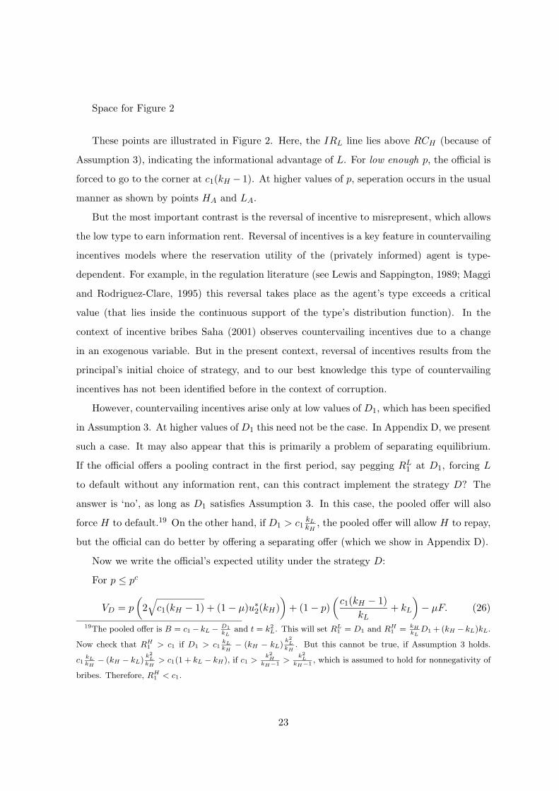
Space for Figure 2

These points are illustrated in Figure 2. Here, the IRL line lies above RCH (because of

Assumption 3), indicating the informational advantage of L. For low enough p, the official is

forced to go to the corner at c1(kH − 1). At higher values of p, seperation occurs in the usual

manner as shown by points HA and LA.

But the most important contrast is the reversal of incentive to misrepresent, which allows

the low type to earn information rent. Reversal of incentives is a key feature in countervailing

incentives models where the reservation utility of the (privately informed) agent is type-

dependent. For example, in the regulation literature (see Lewis and Sappington, 1989; Maggi

and Rodriguez-Clare, 1995) this reversal takes place as the agent’s type exceeds a critical

value (that lies inside the continuous support of the type’s distribution function). In the

context of incentive bribes Saha (2001) observes countervailing incentives due to a change

in an exogenous variable. But in the present context, reversal of incentives results from the

principal’s initial choice of strategy, and to our best knowledge this type of countervailing

incentives has not been identified before in the context of corruption.

However, countervailing incentives arise only at low values of D1, which has been specified

in Assumption 3. At higher values of D1 this need not be the case. In Appendix D, we present

such a case. It may also appear that this is primarily a problem of separating equilibrium.

If the official offers a pooling contract in the first period, say pegging RL1 at D1, forcing L

to default without any information rent, can this contract implement the strategy D? The

answer is ‘no’, as long as D1 satisfies Assumption 3. In this case, the pooled offer will also

force H to default.19 On the other hand, if D1 > c1kLkH

, the pooled offer will allow H to repay,

but the official can do better by offering a separating offer (which we show in Appendix D).

Now we write the official’s expected utility under the strategy D:

For p ≤ pc

VD = p

(2√c1(kH − 1) + (1− µ)u∗2(kH)

)+ (1− p)

(c1(kH − 1)

kL+ kL

)− µF. (26)

19The pooled offer is B = c1− kL− D1kL

and t = k2L. This will set RL1 = D1 and RH1 = kH

kLD1 + (kH − kL)kL.

Now check that RH1 > c1 if D1 > c1kLkH− (kH − kL)

k2LkH

. But this cannot be true, if Assumption 3 holds.

c1kLkH− (kH − kL)

k2LkH

> c1(1 + kL − kH), if c1 >k2H

kH−1>

k2L

kH−1, which is assumed to hold for nonnegativity of

bribes. Therefore, RH1 < c1.

23

For p > pc,

VD =c1(kH − 1)

kH+ p(1− µ)u∗2(kH) +

(p

kHρ

ρ− θkH+ (1− p)kL

)− µF. (27)

Given F not too large, VD(.) is strictly positive, convex, and continuous at all p ∈ (0, 1].

The segment given by (27) is strictly convex. We assume that VD is also increasing in p.20

So far we assumed that D1 < kUc1. What will be the case if D1 ≥ kUc1, while still

maintaining Assumption 3? The official’s optimal offers do not change, but he will face a

greater penalty in the following way. Regardless of whether he was fined in the first period or

not, an incidence of default will attract a high penalty F2. So this additional penalty makes

his payoff smaller:

VD = VD(p)− (1− p)F2. (28)

Needless to say, VD(p) has the same derivative property as VD. But since F2 is large, it is

possible that at some low values of p (say p ∈ [0, pf ]) VD remains non-positive, in which case

the official is better off by not playing the strategy D. Thus setting D1 ≥ kUc1 can be seen

as an effective way of curbing extractive corruption as long as p is small. But its effectiveness

disappears as p is sufficiently close to 1. In this case, VD is close to VD.

Before we proceed to the next section, it will be useful to consider also the strategy of

forcing both types to default- strategy BD. Formulating the problem as a one period problem,

we can check that type H will receive information rent (but only for one period), and the

menu of offers will be similar to that under the strategy R. The corrupt official’s expected

payoff will be:

VBD(kL, kH) = (c1 −D1

kL) + pkH + (1− p) kL

(1 + ρθkL)− µF (29)

if D1 < kUc1 and

VBD(kL, kH) = VBD(kL, kH)− F2 (30)

if D1 ≥ kUc1.

20This will require c2 large and µ small enough to make (1 − µ)u∗2(kH) >[

(2√c1(kH−1)−kl)2

kL

]. See more

discussion in Appendix C.

24

It can be shown that as long as µ is not too large (or alternatively C2 is large, or F is

small), then VR dominates VBD at all p.

VR − VBD(kL, kH) = (1− µ)[c2 −

D2

kL+ kL

]+ (c1 −D1)

[(1− µ)kL − 1

kL

]+pθ

[D2

(1− µ)kL − 1kL

+ kL(1− µ)k2

H − kLkH

]− µ(1− µ)F (31)

If µ→ 1, the above expression clearly becomes negative. On the other hand, if µ→ 0, all

the terms become positive and as long as F is not very high, VR will dominate VBD at all p.

This means that extreme enforcement, which not only causes a small fine F this period, but

also eliminates all future returns, will make the official over-extractive, and the outcome will

be extremely inefficient.

We assume that µ is not so high to allow this perverse possibility. In the case of D1 ≥ kUc1,

high F2 can render VBD < 0 at all p, and the official will not find it worhtwhile to force both

types to default. Therefore we restrict our attention only to strategies D and R.

3.2 Default or Repay?

The two strategies - ‘both repay’ and ‘only H repays’ - have a tradeoff. If both are to repay,

the official must concede a great deal of rent to the H type, but he can expect a large payoff

in the second period. On the other hand, should he make L default, his second period payoff

will be smaller, but he can extract more from H both now and later.

Given that the strategy D is relatively more attractive in the first period, the scale can

tilt in its favor only if p (i.e. the prior on H) is high. When the borrower is more likely to

be highly productive, it may be optimal to maintain a long-term relation with the high type

alone than with both. As does the following proposition show, inducing L to default is indeed

optimal at higher values of p.

Proposition 3 (a) There exists a unique p, say p∗ such that at all p > p∗ the corrupt official

induces the L type to deault. (b) Assuming VR and VD both increasing in p, if V ′R(p) < V ′D(p)

at all p ≤ pc (where pc is defined in Proposition 2), then p∗ is unique, which implies that at

all p ≤ p∗ the official induces repayment by both types. (c) The value of p∗ is higher when

D1 ≥ kUc1, as compared to when D1 < kUc1

25

For proof See Appendix C.

Space for Figure 3

Proposition 3 establishes our central result. The probability of default by a L type bor-

rower is now unconditionally positive. This can be seen from the fact that VD exceeds VR as

p → 1, and VR exceeds VD as p → 0. Then they must intersect at least once. Suppose p∗ is

the highest such value of p among the intersection points. In part (b) we then show that if a

sufficient condition is met, which is favoured by a small µ or large c2, the intersection will be

unique. This means that repayment (default) by type L will occur only at p below (above)

the critical mark p∗. Part (c) extends the same result to the case where a U type is excluded

through higher penalty. Since default will now invite a sure and higher penalty in the second

period, the cutoff probability must rise allowing repayment over a longer range of p.

Figure 3 illustrates this case. As is shown, the VR curve dominates VD only up to p∗. To

illustrate how the information rents matter for this decision, we draw the official’s hypothetical

payoffs, WR and WD, had he not given any rents at any p, and had there been no distortions

in B and t (for each type).21 We see that WR dominates WD over the entire support. While

VD < WD, as is VR < WR, VR falls short much more sharply (at high p) than VD, giving

rise to the above result. Thus, differential screening costs result in the inefficient choice of

the mixed contract over the uniform (long term) contract giving rise to inefficiency. The

screening cost differs between the two strategies because of both of informational ratchet

effect and countervailing incentives. It can be shown that the presence of only one such

factors is enough to cause inefficiency.

Note that for the optimality of default, VD must remain above VR as p→ 1:

VD(1)− limp→1

VR(1) = c1θ + θD2 + k2

L

kH> 0.

Recall from our discussion of equation (11) in Section 3.1.1 that these two terms represent

information rents for two periods. Even if we did not have informational ratchet effect, still

VD would dominate VR by θc1 (static rent). That would be enough to make the make strategy

D (or the mixed contract) optimal.21WR = pUR(kH) + (1− p)UR(kL), and WD = pUR(kH) + (1− p)UD(kL), where UR(.) and UD(.) functions

are given are Section 2.2. Since by Assumption 1, UR > UD for both H and L, WR ≥WD always holds.

26

Conversely, if we did not have countervailing incentives, but only dynamic information

rent, then also default would appear optimal. We prove this point in Section 7. There is a

range of D1, where the reversal of incentive to misrepresent does not occur. For example, at

D1 ≥ kLkHc1, it is the H type who has the inecentive to misrepresent, regardless of whether the

official plays R or D. As we show in Section 7, because of the dynamic rent associated with

the uniform long term contrct, strategy R loses out to strategy D, which requires payment of

only one period rent.22

It is straightforward to calculate the probability of default (in the first period) conditional

on kl being kL, as:

σ(p | kL) = 0 for p ≤ p∗

= (1− q)(1− p) for p > p∗

The above analysis lends some support to the view that the long term effect of corruption

is much more harmful than its short run incentive effects. We identify a particular type

of inefficiency - corruption induced default - that may have a greater social implications.

Rose-Ackerman (1999) and many other authors have therefore warned against soft policies

on corruption.

To sum up, we have shown that offering a short term contract to a low productivity type

can be optimal when the prior on the borrower being high productivity is on the higher

side. The key reason for such optimality is the cost of screening the borrower’s type. From

a corrupt official’s point of view, offering long term contracts to both types of borrowers

may involve yielding dynamic information rents to the high productivity type. But offering

a mixed contract (invloving a short term contract to the low type and a long term cotract

to the high type) will eliminate dynamic rents, and further may even allow pegging the high

type to his minimum payoff. This is why the mixed contract is optimal, when the borrower

is more likely to be a high type.22Here, it is noteworthy that our argument goes through even if separating equilibrium did not exist under

repayment. In that case the official would resort to pooling offers at all or some p. But that would have yielded

a lower VR curve, and consequently a smaller p∗, which implies even greater inefficiency.

27

3.2.1 Comparative statics

In light of the Proposition 3, we can say that, p∗ ≥ p is a new repayment incentive condition

appropriate for a corrupt official constrained by asymmetric information, because it restates

VR(p∗;α) ≥ VD(p∗;α), where α is the vector of parameters (notably, c1 and c2).

How does the critical value, p∗, change with the loan terms or anti-corruption measures?

The answers are unambiguous and interesting. Suppose D1 < kUc1, p∗ > pC and it is

unique.23 Then we can write,

VD(p∗(α))− VR(p∗(α)) ≡ 0,

where α = (c1, c2, D1, D2, F, µ). This leads us to:

∂p∗

∂α=

[∂VR∂α −

∂VD∂α

]V ′D(p∗)− V ′R(p∗)

.

Since V ′D(p∗) > V ′R(p∗), the sign of ∂p∗

∂α is given by the sign of [∂VR∂α −∂VD∂α ].

It is straight forward to check that,

∂p∗

∂c1< 0,

∂p∗

∂c2> 0,

∂p∗

∂D1> 0,

∂p∗

∂D2< 0,

∂p∗

∂F< 0,

∂p∗

∂µ< 0.

An increase in p∗ means an improvement in the prospect of repayment. It is not hard to

see why the present and future loan terms affect the repayment prospect in opposite ways.

The corrupt official induces repayment in order to appropriate the second period surplus

(kc2−D2) of the borrower by paying him k(c1−D1), what he could have got by defaulting in

the first period, (recall condition (1)), plus some information rent, if necessary. An increase in

c1 thus reduces the official’s payoff and makes repayment a less attractive option. Therefore,

p∗ falls. In contrast, an increase in c2 directly increases the pie that he appropriates in the

second period. Hence, its effect of p∗ is positive. Analogous reasonings can be applied to D1

and D2. But more interestingly, the effect of stricter anti-corruption measures are seen to

be counter-productive, as was seen under symmetric information. A small increase in F or

µ, reduces the official’s expected payoff from repayment much more than that from default.

Hence, the prospect for default rises.23The case of D1 ≥ kUc1 is similar, and signs are identical.

28

4 The case of kU

We now consider the case where kU is realized instead of kL. Since kU is strictly less than

1, advancing loan to U is socially inefficient. This inefficiency can be resolved by setting

D1 ≥ kUc1, in which case the only borrower to approach the official must be the H type. The

corrupt official can easily extract full information payoff from the borrower, and will always

induce repayment.

But he may not be able to do so, if D1 < kUc1, because now U will also take the loan

along with H, and the informational uncertainly will come back. In the case of an honest

official, as before the borrower receives the loan at no cost, and U will default. With a corrupt

official it remains to be seen whether H type will also default or not.

Formally, we consider two strategies of the official: ‘both types default’, BD and only

‘U defaults’ (strategy UD). When both types default, the problem reduces to a one period

problem, where the borrower’s gross payoff must be at least D1. It can be easily seen that

type H will have to be given one period rent to reveal his type, while type U is pinned down

to zero profit. Following the analysis of Section 3.1.1, we derive the official’s expected payoff

from strategy BD as:

VBD = (c1 −D1

kU) + pkH + (1− p) kU

(1 + ργkU )− µF (32)

where γ = 1kU− 1

kH. VBD(.) is continuous, increasing and convex in p.

On the other hand, when the official wishes to make H repay (while U defaults), the

size of D1 matters for which type to be given rent. We consider two scenarios: First, D1 ∈

[ kUkH c1, (1 + kL − kH)c1), i.e. when D1 is not small. Second, D1 < (1 + kU − kH)c1) < kUkHc1.

Note that D1 = 0 is a special case in the second scenario. Very poor borrowers may fall in

this category. We shall see that the outcomes are quite different between these two cases.

The case of D1 >kUkHc1: In this case making R repay will entail transferring rent to him.

Therefore, in terms of bribe and red tape it is similar to BD strategy, but now there is a

second period payoff. Thus,

VUD = VBD(kU , kH) + p(1− µ)u∗2(kH).

Obviously, in this case H will never be induced to default. But that is not so in the next case.

The case of D1 < (1 + kU − kH)c1): Now the informational advantage switches in favor

of U , exactly the same way observed in Section 3.1.2. Consequently, the official’s expected

29

utility VUD will be identical to (26) and (27) with kL being replaced by kU , θ by γ and pc

by pU , where γ and pU are redefined in terms of kU . A direct comparison between VBD and

VUD gives the following result.

Proposition 4 Assume 0 < (1 + kU − kH) < kUkH

. If D1 ≥ kUkHc1, inducing H to default is

never optimal. But if D1 < (1 + kU − kH)c1, there exists a critical p, say p, such that at all

p < p, H will be made to default along with U . At all p ≥ p, the H type repays. Assuming

VUD increasing, if V ′BD(p) < V ′UD(p) at all p ≤ pU , p is unique.

For proof see Appendix D.

While the above proposition points to the possibility of greater inefficiency as the high

productivity type may also fail to repay, the reason for inefficiency is still the same. The

corrupt official’s tradeoff between a mixed contract and a uniform contract is critical. Note

that here the uniform contract is a menu of short term offers to both types, and thus, there

is no room for dynamic information rent. So, for the inefficient treatment of H , we must

need countervaling incentive. If D1 is high, there are no countervalining incentives, and H

is induced to repay at all p. Here, the mixed contract wins over the uniform contract. But

if D1 is low either because the government is generous, or because the borrower is poor,

countervailing incentives arise between the two contracts, and as before the mixed contract

wins over the uniform contract at higher values of p, which in this case implies ‘efficiency’

(because H reapys). But at smaller values of p, the consequence is disastrous. The high

productivity borrower also turns defaulter.

The probability of default, conditional on kl being realized as kU , is:

σ(p | kU ) = (1− q) + q(1− p) for p < p

= (1− p) for p ≥ p

What are the comparative static properties of p? Following the same procedure as in the

previous section, it can be shown that the sign of ∂p∂α is given by the sign of [∂VBD∂α − ∂VUD

∂α ].

Again using (32) and the convex segment of VUD it can be shown that,

sign of ∂p∂α = - sign of ∂p∗

∂α .

30

The effect of α may appear exactly opposite of what we have seen earlier, but it is actually

working in the same direction. For example, an increase in c1 will increase the chance of H

defaulting when kU is realized, and will also increase the chance of L defaulting when kL is

realized. Greater c1 reduces the official’s future payoff comparatively more than it increases

his current payoff. Hence, the inefficiency. Formally, of course, the two cutoff probabilities,

which are essentially two repayment incentive conditions from a corrupt official’s point of

view, will tend to move apart, if c1 is reduced, or c2 is increased. This is important, as we

shall see, for the optimal design of the credit program.

5 Optimal credit program

In this section, we would like to model the government’s choice over the elements of α =

(c1, c2, D1, D2, µ, F ) that can influence the outcome of the game by raising the probability of

repayment, p∗(α). In attempting such an analysis, we choose the following objective function:

Government’s objective: Z = Expected payoff of the borrower - expected subsidy cost -

expected monitoring cost.

This is sought to be maximized, subject to a number of constraints that may reflect the

strategy of the government, institutional flexibility in tackling corruption and availability of

credit.

First consider the outcome that is efficient from the repayment point of view: if a loan is

advanced, it is never defaulted. How does the government ensure this outcome?

We first consider the ideal scenario, where the official is known to be honest, all U type

borrowers can be excluded by setting D1 equal to kUc1, and D2 can be raised to c2 to

eliminate the default problem in the second period as well. The credit program optimal to

this environment should be seen as the first best program.

The social welfare function Z will consist of the following expected payoff of the borrower:

X1 = pΠ(kH) + (1− p)βΠ(kL)

where Π(.)-s are given by (4). Note that a U type does not take the loan.

31

Now consider the subsidy cost. When the loans are repaid, subsidy cost consists of only

interest. For the first period it is rc1, which after one period becomes rc1(1+r) where r is the

government’s opportunity cost of fund. If the borrower defaults, then not only the interest,

but also a part of the principal, (c1−D1) = c1(1−kU ), is also lost. The second period subsidy

is c2r.

The subsidy cost in an honest regime is:

Y1 = p+ (1− p)β [c1r(1 + r) + c2r]

Finally, since there is no corruption, the monitoring cost is zero.

Assuming that D1 = kUc1 and D2 = c2, the government’s problem can be stated as:

Maximize with respect to c1, c2 :

Z = X1 − Y1

subject to:

c2 ≥[

(1− kU )kL(kL − 1)

]c1 (33)

c1 ≤ c1

c2 ≤ c2.

The first constraint is a restatement of condition (3), which ensures that H and L will not

willfully default. The second and the third constraints are simply the availability constraints.

Note that the social welfare function and the constraints are all linear. Therefore, we

are going to get corner solutions. Assuming ∂Z∂c1

> 0 and ∂Z∂c2

> 0 on regularity grounds,

two possibilities are noted. If c2 ≥ [ (1−kU )kL(kL−1) ]c1, then c1 = c1 and c2 = c2. Otherwise,

c1 = c2[ (kL−1)kL(1−kU ) ] (denote it as c1(c2)), and c2 = c2. The basic point is that the government

will make the loans as large as possible, as long as they satisfy the no-willful-default constraint.

This is our first best credit program.

In the general case, the first best may not be implementable, for two reasons: (1) corrup-

tion, (2) difficulty of excluding U type borrowers. If the borrowers are poor, exclusion of U

may not be feasible. In that case, an incidence of default cannot be attributed to corruption,

and the official cannot be punished accordingly. The wealth constraint of the borrower may

further restrict the size of D2.

32

We consider a particular case of very poor borrowers, where D1 = 0, but D2 > 0. Since

D2 does not play an important role we set D2 = c2 for simplification.

Now, the government has to choose (c1, c2) by paying attention to two more constraints.

To ensure that both H and L repay when kL is realized , p∗(α) should be set at least equal

to p, and to ensure that H repays when kU is realized, p(α) must not exceed p. These two

are the appropriate repayment incentive conditions for a corrupt regime involving all three

types of borrowers.

While the above problem looks at an efficient outcome, an inefficient outcome involving

default by L can also be considered. This will require violating the constraint p∗(.) ≥ p. We

would like to compare the designs of the credit programs for these two different outcomes,

and see if ever the inefficient outcome is preferred.

In order to state the problem formally, we need to specify the monitoring cost. It is

not unreasonable to suppose that the monitoring operation is self-financing. Suppose the

government chooses µ such that M = 0.24 To simplify further, we assume that F and F2 are

exogenously given.25

Let X2 denote the borrower’s expected payoff under corruption and Y2 the expected

subsidy cost under corruption. Since these expressions are lengthy, we relegate them to

Appendix E. The government’s problem is to choose (c1, c2), which maximizes

Z = qX1 + (1− q)X2 − qY1 − (1− q)Y2

subject to the following constraints:

p∗(c1, c2, D2(c2)) ≥ p (34)

p(c1, c2, D2(c2)) ≤ p (35)

c1 ≤ c1

c2 ≤ c2.

24Suppose, the investigating agency, if called to investigate, is paid an exogenous fee M . When not called,

it gets nothing. From investigation the government’s total expected revenue is µ(1− q)F + (1− µ)(1− q)F =

(1 − q)F , but it must pay µ[M + (1 − q)M ] + (1 − µ)M . Thus, the expected cost equals M [1 + µ(1 − q)].

Setting expected cost equal to expected revenue, we get µ = FM− 1

(1−q) . For µ > 0, F must exceed M .25F is likely to be related to the salary of the official. F2 can be severe in the sense of being transferred to

a different location, or it can be a jail term also.

33

Note that the no-willful default constraint (33) is now replaced by two probability con-

straints. The first one is to ensure that L does not default and the second one will ensure that

H does not default when U is present. As we know these two constraints are much stronger

than the no-willful default constraint (compare (3) and (6)). Under corruption (6) must be

satisfied, and therefore, the no-willful default constraint is automatically satisfied.

First consider the repayment outcome. Setting the Lagrangian appropriately and assum-

ing that the second order conditions hold, we state the key first order conditions:26

c1 :∂Z

∂c1+ λ1

∂p∗

∂c1− λ2

∂p

∂c1− λ3 = 0 (36)

c2 :∂Z

∂c2+ λ1[

∂p∗

∂c2+∂p∗

∂D2

∂D2

∂c2]− λ2[

∂p

∂c2+

∂p

∂D2

∂D2

∂c2]− λ4 = 0 (37)

where λi, (i = 1, 2, ..., 4) are the Lagrange multipliers for the i-th constraint. Other first order

Kuhn- Tucker conditions for the λ-s are ommitted.

While the formal solution is given in Appendix E, here we present an informal discussion.

We first ask: Is the first best solution ever admissible? The answer is ‘No’. If it were true,

then L can never repay when the official is corrupt.

The optimal solution hinges on the requirement that p ≤ p ≤ p∗ must be maintained in

equilibrium, and for that reason c1 and possibly c2 will have to be distorted. Here, the effects

of c1 and c2 on p and p∗ are important. We know from our discussions in sections 3.2.1 and

4 that c1 negatively affects p∗, but positively affects p. It can also be shown that the total

effects of c2 - direct and indirect (via D2) - on p are negative, but ambigusous for p∗.27

Space for Figure 4

These signs play a crucial role and ensure that in general only one of the two probability

constraints will bind. Consider a very low value of p. To hold p below p, c1 is to be reduced,

while c2 is to be raised. Thus, c2 is to be held at c2, and c1 is to be adjusted to set p = p.

This also helps to keep p < p∗. Clearly, to maintain p = p with lower p, c1 must fall and

symmetrically with higher p, c1 will rise. However, as shown in Figure 3, beyond a point where26For the fulfillment of the second order condition, it is required that p ∗ (.) and p(.) be quasi-concave in

(c1, c2).27[ ∂p

∂c2+ ∂p

∂D2

∂D2∂c2

] is given by the sign of [−p(1−µ) (kH−1)kH

]. But the sign of [ ∂p∗

∂c2+ ∂p∗

∂D2

∂D2∂c2

] depends on the

sign of [(1− µ)(1− p) (kL−1)kL

− θpkH

], which can be positive (or negative) depending on whether p falls short of

(or exceeds) pµ = (1−µ)(kL−1)kH(1−µ)(kL−1)kH+θkL

.

34

the gap between p and p∗ disappears, c1 cannot be increased. If c1 is rasied further p∗ will fall

below p, and L will be made to default. Suppose c1 is such that p(c1, c2) = p∗(c1, c2) = p0.

Then at all p > p0, c1 must be decreasing in p to maintain the equality p∗(.) = p. But here c2

may not necessarily be held at c2, because the total effect of c2 on p turns negative at some

p > pµ. Suppose pµ > p0. Then beyond pµ we arrive at an interior solution of the following

kind:

∂Z∂c1∂Z∂c2

=[∂p∗

∂c1+ ∂p∗

∂D1kU ]

[∂p∗

∂c2+ ∂p∗

∂D2]

(38)

This is a familiar tangency solution when the government is maximizing a linear (expected)

social welfare function subject to a quasi-concave iso-probability function p∗(.) which is set

equal to p. Optimal (c∗1, c∗2) will lie within their bounds. Consequently, the differnce between

the two credit amounts may get smaller.

But how far is repayment possible? It can be checked that p∗(.) will not go to 1, even if

c1 → 0. We have noted that limp→1[VD − VR] = θ

[c1 + D2+k2

LkH

], does not go to zero if we let

c1 go to zero. Suppose p∗ goes to some limiting value p+ < 1. Then beyond p+ the repayment

strategy is not feasible.

In Figure 4, we draw optimal c1 against p. Suppose p(c1) = p and p∗(c1) = p can be

inverted to write c1(p) and c∗1(p) respectively. The two curves move in exactly opposite

directions. In order to maintain p∗ ≥ p, c1 cannot be raised beyond c01. This gives rise to an

inverted U-shaped c1-curve. Optimal c2 is held constant at c2 at all p up to pµ, but afterwards

c2 also falls.

How will the social welfare function look like in this case? Figure 4 shows that ZR should

be increasing in p up to p0 and then should decrease, as the credit amounts fall.

Next, we consider the inefficient outcome where the government may permit L type to

default, which occurs if p∗() < p. This effectively requires violating the first constraint. So

if the government continues along the c1(p) curve with c2 = c2, the L type would default at

all p > p0. Therefore, when default by L is permitted, the optimal credit progarm is simply

given by (c1(p), c2). Since c1 is increasing, ZD will also be an increasing function; but because

of default, ZD will start from a much lower value than ZR at p0. Eventually ZD crosses ZR

at a point like p as shown in Figure 5. Therefore, permitting default will be optimal at all

p > p. If ZD and ZR do not intersect, then p = p+.

35

Proposition 5 There is a critical p, say p such that at all p > p, it is optimal for the

government to permit default, but maintain an increasing profile of c1 while c2 is held at its

maximum. But at all p ≤ p it will adopt a default-proof credit program, but at the cost of

reducing c1 to a substantially low level.

Space for Figure 5

Finally, it may be asked how the design of the optimal credit program would change if the

government could adjust D1 freely to keep the U type out of contention. If D1 could be set

equal to kUc1, then constraint (35) would be irrelevant, and H will always repay. To ensure

that L repays, c1 must be given by c∗1(p), which is all through declining. Consequently, ZR

will also be declining. The default strategy on the other hand requires setting a constant

c1, which should be equal to c1(p = 0) at all p. Such a c1 will permit repayment by L only

if the borrower is surely the low type. Because of high and constant c1 and c2, (= c2), ZD

will be increasing. But now the penalty is severe (F2). Therefore p will be greater, but still

strictly less that 1. Thus, even if U could be excluded, the problem of default cannot be fully

eliminated.

Thus, two aspects appear to be integral. First, though the government can significantly

improve the repayment prospect by appropriately designing the loan sequence, the default

problem cannot be fully eliminated. In fact the probability that it will settle for an inefficient

outcome (by tolerating default) is strictly positive. Second, under-provision of the first period

credit seems a natural way to reduce the default probability. Here, we must note that the

divergence from the first best level of credit provision occurs due to two reasons: corruption

and asymmetric information. If there was no informational uncertainty, then c1 still needs to

be reduced below the first best level, but repayment can always be ensured. But asymmetric

information introduces an additional source of inefficiency, and beliefs about the borrower’s

types begin to play a critical role. Ensuring repayment requires further under-provisioning of

the first period credit.

36

6 Extension I: Moderate D1 - the case of countervailing incen-

tives

In this section we consider some interesting extensions. An increase in D1, collateral or

penalty on default, may not necessarily improve efficiency, unless U is excluded. As we show

higher D1 can change the default strategy in an interesting way; the official can deny the

agent of any information rent, as the agents face countervailing incentives.

Here we drop Assumption 3, and let D1 be greater than c1(1 + kL − kH). However,

this generalization affects only the strategy of default (i.e. only L defaults). The ‘both

repaystrategy’ does not change.

To understand the role of Assumptions 3 let us recall the basic feasibility constraints -

repayment constraint for H and individual rationality constraint for L from the problem P’:

(RCH) : tH + c1 ≤ kH(c1 −BH)

(IRL) : tL +D1 ≤ kL(c1 −BL)

It can be readily checked that if D1 < c1(1 + kL − kH) and D < c1kLKH

, the IRL curve will lie

above the RCH curve on the (t, B) plane. That is, the feasible set of offers for L will be larger

than the feasible set of offers for H. This implies that L will have a systematic incentive to

misrepresent and this was ensured by Assumption 3, since kLkH

> (1 + kL − kH).28

If D1 > (1 + kL − kH)c1, no longer will RCH lie below IRL. Instead, the two curves will

intersect and then we may suspect that L’s incentive to misrepresent will not be uniform (or

systematic). Indeed with changes in D1, the informational advantage gradually moves away

from L to H revealing a pattern of countervailing incentives.

As is typically the case in such models, the two constraint (RCH and IRL) intersects,

and their intersection point will vary with D1 (as we hold other parameters unchanged). In

Figure 6, two intersecting constraints are drawn. Let the intersection point E be given by

(t, B), where it is straight-forward to check:

t =(c1kLkH−D1

)kH

(kH − kL), (39)

28Rewrite (1 + kL − kH) ≤ kLkH

as k2H − kH(1 + kL) + kL ≥ 0. Setting it as equality, we can show that the

resulting quadratic equation has two real roots: 1 and kL. So this inequality is violated if kH ∈ (1, kL). But

by assumption kH > kL. So, kLkH

is always greater than (1 + kL − kH).

37

B =D1 − c1(1 + kL − kH)

(kH − kL). (40)

Note that the intersection point varies with D1, and it is strictly in the interior if D1 ∈

(c1(1 + kL − kH), c1kLkH

). In the ensuing analysis the relative position of the full information

offers (in comparison to point E) is going to be crucial.

Insert Figures 6 and 7 here.

For instance, if the full information solutions for H and L are given by points A and

B, then we will have a different incentive regime than if they were at points C and F . By

incentive regime we mean which type has the incentive to misrepresent had they been given

the full information offers for the same strategy of the official.29 How the point E will shift

vis-a-vis the full information offers depends on the size of D. Since full information tH∗

= k2H

and tL∗ = k2L are independent of D1, by comparing them with t we can easily identify the

critical values of D1, which give rise to three incentive regimes.

Define D∗1 such that for all D1 > D∗1, the full information red tape tH∗ is greater than t.

D∗1 is obtained by setting t = tH∗:

D∗1 = c1kLkH− kH(kH − kL). (41)

Similarly, define D∗∗1 such that for all D1 > D∗∗1 , the full information red tape tL∗ is greater

than t. D∗∗1 solves t = tL∗. It can be readily checked from the following expression as well as

from Figure 7 that D∗∗1 > D∗1.

D∗∗1 = c1kLkH− k2

L

kH(kH − kL). (42)

Figure 7 shows how these critical values of D1, which help to determine the relative

positions of the full information offers vis-a-vis (t, B). As D1 starts rising towards D∗1, the

gap between tH∗ and t narrows, but t still remains higher. This will correspond to offers given

by points A and B in Figure 6, such that the configuration becomes tL∗ < tH∗ < t. Once this

is understood, it becomes obvious that in this situation the low type will have incentive to

misrepresent and the full information offers must be distorted to induce truth telling.29For L it is not exactly the full information offers, but the offers under full information corresponding to

the default strategy.

38

Similarly, when D∗1 < D1 < D∗∗1 , the configuration becomes tL∗ < t < tH∗, which may

correspond to offers given by points like A and C in Figure 6. Here, interestingly the full

information offers are incentive compatible. Thus, with the help of Figures 6 and 7 we can

identify the following incentive regimes.

1. Regime 1: Type L has incentive to misrepresent if D1 < D∗1. This is just a continuation

of the same incentive regime that we have analyzed in section 3.2. Therefore, the

optimal offers will be same as in Proposition 2 except for the corner solution, which is

now modified as (t, B) and the critical value of pc should also be modified accordingly.

But what is most interesting is that when the corner solution occurs (i.e. at (t, B)),

both the RCH and IRL bind simultaneously, meaning that the first period net payoffs

of both types will be zero.

2. Regime 2: None has incentives to misrepresent if D1 ∈ [D∗1, D∗∗1 ]. In this case, the

official will make the full information offers. Moreover, H’s offer will lie outside the L’s

feasible set, and L’s offer will be outside H’s feasible set, as shown in Figure 6 by points

A and C. So there is no incentive problem here.

3. Regime 3: If D1 > D∗∗1 , type H has incentive to misrepresent. With even greater value

of D1, t will fall below tL∗ and L’s offer will be inside H’s feasible set. However, while

L’s red tape will be reduced to lower the information rent, it will never be less than t,

and if tL hits t, then H will also be pushed to his repayment constraint.

We make these regimes precise in the following proposition.

Proposition 6 1. Suppose D1 ∈ [c1(1 + kL − kH , D∗1). (a) For p > pc′

=√t√

t−kLθkL, the

optimal offers are same as in equations (20)-(23). (b) For p ≤ pc′, tH = t, BH = B,

tl = tL∗ and BL = BL∗, resulting in RH1 = c1 and RL1 = D.

2. When D ∈ [D∗1, D∗∗1 ], optimal offers are: ti = k2

i , i = H,L and BH = c1 − kH − c1kH

,

BL = c1 − kL − DkL

, ∀p ∈ [0, 1].

3. Assume D1 ∈ (D∗∗1 , c1kLkH

]. (a) For p < pc′′

=(kL−√t

kH−√t

)kHkL

, the optimal tH , tL are

same as in Proposition 1 (equations (12) and (14) respectively), and since the low type

39

defaults, optimal BH , BL are given by:

BH =[c1

(kH − 1)kH

− kH]−[θ(c1 +

k2L

(1 + ρθkL)2)

](43)

BL = c1 −kL

(1 + ρθkL)2− D1

kL. (44)

(b) For p ≥ pc′′, tL = t, BL = B, tH = tH∗, and BH = BH∗. In this case, RH1 = c1

and RL1 = D1.

4. If D1 ∈ (c1kLkH, c1], the optimal offers are same as in part (3.a) for all p.

For proof see Appendix F.

The proposition shows how the red tape and bribe will vary with changes in the exogenous

penalty and the official’s priors. More appropriately, the default strategy is characterized by

several incentive regimes. For a more useful discussion, we can fix p and examine the interior

solution as it changes with D1.

At low values of D1, the red tape for H is given by equation (21) or tHA as shown in Figure

8, and the red tape for L is at the full information level tL∗. As D1 reaches D1, which is

given by the equality of tH as in (21) and t, the red tape for H will be restricted at t and

will continue to be so till D∗1. Particularly in this phase, the red tape is clearly sensitive to

the penalty. After this the red tape again becomes insensitive to D1, but it settles down at a

lower level at tH∗. Similarly the red tape of the low type can be understood.

Thus, it appears that when the official prefers to play the default strategy (i.e. only

L defaults), the penalty on default reduces the expected delay or red tape in an indirect

manner, primarily through regime changes. As the penalty increases from low to moderate

and to higher levels, red tape eventually falls for both types - from tHA to t and then onto tH∗

for H, and from tL∗ to tLA via t for L. This can be described as an efficiency effect of the

policy of increasing penalty on default.

However, a related question is: does it increase profit for the borrower? This relates to

information rent accumulation or rent dissipation. As is well known, countervailing incentive

models typically exhibit a phase of rent dissipation, and our model is no exception. The

only difference in our case, as compared to Lewis and Sappington (1989) and Maggi and

40

Rodriguez-Clare (1995), is that the rent dissipation is triggered by a change in an exogenous

variable. This is similar to Saha (2001). In Proposition 6, we have shown how the first

period net profits (or information rent) of the borrower will change. The rent will completely

disappear in regime 2, but will come back in regime 3.

To emphasize on the rent dissipation process, we state it more formally in our next propo-

sition, and also provide a visual illustration in Figure 8. The information rent of the low type,

which is given in Proposition 2 is declining in D1. But it is strictly positive until D1 reaches

D1. Thereafter it is zero. It is noteworthy that for all D1 < D∗1, the low type has incentive to

misrepresent (Regime 1). But this incentive is not uniformly strong or profitable. It weakens

gradually. In fact, the incentive becomes completely useless well before D∗1 at D1.

Similarly, the high type has incentive to misrepresent in Regime 3, at D1 > D∗∗1 . But it

does not translate into rent immediately at D∗∗1 . Only from D1 the high type begins to enjoy

rent, which however increases with D1. Thus, the entire interval [D1, D1], which includes

Regime 2 well inside, is marked by complete dissipation of information rents.30

Space for Figure 8

Proposition 7 For a given p there exists an interval of D1, say [D1, D1], where c1(1 + kL−

kH) < D1 < D∗1 and D∗∗1 < D1 < c1kLkH

, such that at all D1 ∈ [D1, D1], the first period net

profit (π1) is zero for for both types of the borrower. Moreover, πL1 > 0, for D1 < D1 and

πL1 = 0, ∀D1 ≥ D1. Similarly πH1 > 0 for D1 > D1 and πH1 = 0, ∀D1 ≤ D1. Formally,

D1 = c1kLkH− kH

(ρ

ρ− θkH

)2

(kH − kL) (45)

D1 = c1kLkH−(

kL(1 + ρθ)

)2 (kH − kL)kH

. (46)

The proof of this proposition is straight forward and therefore ommitted.31 It is now clear

that the default strategy is very attractive when the penalty is moderate, as it involves very30Recall from Proposition 2, πL1 = BH(kH − kL) + [c1(1 + kL − kH −D1)] and with the help of Proposition

1 we can derive πH1 = [c1 − BL](kH − kL) where BL as shown in equation (44) is inversely related to D1.

Therefore, πL1 is inversely and πH1 is directly related to D1.31It is easy to check that D1 > D1. Consider the second term in each equation. The second term in (45) is

41

little information rent or none at all. Although we do not carry out a formal comparison with

the repayment strategy, it can be speculated that with moderate D1 the official’s incentive

to inflict default witll increase. In simpler terms, in Figure 3 the VD curve will be at a much

higher level than if D1 was small. Clearly, the range of p for which the outcome will be

inefficient (or default-prone) will now be greater.

7 Extension II: High D1 - the ratchet effect alone causing de-

fault

Here we consider the case of D1 >kLkHc1 > (1 + kL − kH)c1. This is an interesting case where

the default strategy does not involve countervailing incentives. It is the H type, who will

enjoy the informational rent as in the case of strategy R. The moot point of this exercise

is to show that even when there are no countervailing incentives, ratchet effect (or dynamic

rent) can render the repayment strategy suboptimal.

The official’s problem is:

Max V = p(BH + 2√tH) + (1− p)(BL + 2

√tL) + (1− µ)pu∗2(kH)− µF

subject to

(ICH) : kHBH + tH ≤ kHBL + tL

(ICL) : kLBL + tL ≤ kLBH + tH

(RCH) : kHBH + tH + c1 ≤ kHc1

(RCL) : kLBL + tL +D1 ≤ kLc1

The official’s offers are as follows:

BH =[c1

(kH − 1)kH

− kH]−[θ(c1 +

k2L

(1 + ρθkL)2)

](47)

tH = kH2 (48)

BL =(c1kL −D1)

kL− kL

(1 + ρθkL)2(49)

tL =k2L

(1 + ρθkL)2. (50)

simply tHA(kH−kL)

kH, where tHA is given by equation (21). The second term in equation (46) is tLA

(kH−kL)kH

, where

tLA is given by (14). Since tLA < tHA , D1 < D1.

42

The official’s (undiscounted) two-preiod expected utility is:

VD = p

[c1(kL − 1)

kL

]+ (1− p)

[(c1kL −D1)

kL

]+ p(1− µ)u∗2(kH)

+[pkH + (1− p) kL

1 + ρθkL

]− µF

As p→ 1,

VD =c1(kL − 1)

kL+ kH + (1− µ)u∗2(kH)− µF,

and as p→ 0,

VD =(c1kL −D1)

kL+ kL + (1− µ)u∗2(kL)− µF,

In contrast, recall VR, as given in (17). As p→ 1,

VR =c1(kL − 1)

kL+ kH + (1− µ)u∗2(kH)− θD2 + k2

L

kH− µF,

and as p→ 0, we have

VR =c1(kL − 1)

kL+ kL + (1− µ)u∗2(kL)− µF.

Comparing the above expressions, we see that limp→1 VD > limp→1 VR unambiguously. On

the other hand, limp→0 VR > limp→0 VD if u∗2(kL) > (c1−D1

(1−µ)kL, which is precisely our Assumption

1. Hence this is also true. Then we can argue that these two curves must intersect at least

once. That is enough to prove that at some p default will be preferred.

Note that the key part of our argument, VR(1) < VD(1), is entirely due to the second

period rent. Thus, it is the ratchet effect alone that is causing inefficiency.

Proposition 8 When kLkHc1 < D1 < c1, there will be no reversal of incentive to misrepresent

on the borrower’s part, as the official switchees from repayment to default strategy. Still the

ratchet effect alone makes default optimal at higher values of p.

8 Conclusion

In this paper we have presented a dynamic model of credit provision to examine how asym-

metric information exacerbates inefficiency generated by corruption. A perfectly productive

borrower may be induced by a corrupt official to default, an outcome, which the official would

not prefer under symmetric information. The government can reduce this inefficiency, but

43

will have to reduce the supply of credit. Two factors in our model, informational ratchet

effect and countervailing incentives, which are commonly associated with many agency rela-

tionships, are acting jointly or alone to cause default and in turn under-provisioning of credit.

The countervailing incentive problem can be avoided by placing a substantial collateral re-

quirement. But in the context of offering subsidized credit to poor borrowers, this may not

be feasible. Informational ratchet effect, however, is unavoidable as long as the borrower’s

productivity is unchanged over time. Thus, there is no clear policy choice for the government,

except that corruption needs to be dealt with much more firmly. If the official is honest, or

if honesty can be induced by harsh anti-corruption measures, asymmetric information would

hardly matter. The first best credit program can be implemented.

Now in light of our model, we would like to comment on some of the empirical findings.

As said at the outset, our analysis concerns those cases where the loan official has substantial

bargaining power and the borrowers are at his mercy. Default in such cases is common, and to

what extent corruption can cause it, can be understood with our model. But there is another

group of defaulters, who by the use of their political power and wealth, force the loan official

to divert credit to them. Can our model explain this type of default? Since such borrowers

are likely to have greater bargaining powers, the honesty of the official does not matter. Their

default decisions can be explained to some extent by the basic no-willful-default condition

(3), with two caveats. First, a powerful borrower may influence the official to weaken the

penalty D1 applicable to him. This can upset the inequality in favor of default. Second, this

borrower may have multiple borrowing opportunities, unlike poor borrowers. Default in one

bank may not deter him from future loans offered by another bank.

We have also assumed that the official remains in office for two periods. However, trans-

ferring officials from one place to another is a common practice. Effect of tenure stability

on corruption is an important issue. Choi and Thum (2003) examined how tenure stability

of a corrupt official affects corruption. In our model, if the official knows that he may be

transferred with some probability, then the long-term contract loses its attractiveness, and

the short-term contract will be preferred. In other words, transfer policy will generate greater

inefficiency. However, we must add one qualification. In our model, the official knows that

the borrower cannot influence the probability of investigation by reporting corruption. Sup-

pose that we drop this assumption and allow the borrowers to vary in terms of their ability

44

to influence µ (or provide hard evidence). Shorter duration of tenure in that environment

translates into a greater uncertainty about µ. Consequently, the official may be compelled to

be less extractive in order to generate a lower probability of investigation.

Finally, we did not consider production uncertainty, which is a common assumption in a

credit model. Introduction of this assumption would certainly make our model more general.

We still show that informational uncertainty can lead to a situation where the borrower

defaults, because he is rendered ‘unable to repay’, and not because he is ‘unwilling to repay’.

Appendix A

Proof of Proposition 1. (a) Assume that separating equilibrium exists. Then it can

be shown that of the four constraints only ICH and RCL will bind. This proof is standard,

and therefore omitted. Substitute the expressions for BL and BH obtained from ICH and

RCL into the official’s objective function, and then carrying out maximization, obtain the

first order conditions (11)-(14).

(b) Straight-forward substitution of optimal (B, t) obtained in (a) will yield these profit

expressions.

Alternatively, first rewrite the ICH and ICL in terms of net (post-repayment) first period

profit πH1 and πL1 (by subtracting c1 from both sides, and then assert the following:[πH,L1 + θ(D2 + k2

L)]− πL,L1 ≤ πH,H1 − πL,L1 ≤ πH,H1 − πL,H1 (51)

This inequality simply follows from the incentive constraints. As before πi,j1 refers to the

first period net profit of type i when it misreports as j. Substituting πi,j1 = ki(c1−Bj)−tj−c1,

i, j = H,L, we obtain:

θ(D2 + k2L) + (c1 −BL)(kH − kL) ≤ πH,H1 − πL,L1 ≤ (c1 −BH)(kH − kL)

Since kH > kL, the above inequality implies BL > BH . Moreover, the first part of the

inequality suggests:

πH1 ≥ πL1 + (c1 −BL)(kH − kL) + θ(D2 + k2L). (52)

where πH1 ≡ πH,H1 and πL1 ≡ πL,L1 . The official will maximize his expected utility, by setting

πL1 = 0, and raising BL and BH while maintaining BL > BH , such that the above inequality

holds with equality. The rest follows. QED

45

Appendix B

Proof of Proposition 2. (a) In analogy with the proof of Proposition 1, it can be shown

that at the optimum only RCH and ICL will bind, and BL ≥ BH must also hold. Next,

substituing RCH and ICL into the objective function, and maximizing it we get (??)-(??).

However, for BH > 0, we need

c1(kH − 1)kH

> kH(ρ

ρ− θkH)2

which gives rise to the restriction: p > pc. For p ≤ pc, BH must be zero. This reasoning gives

(18) and (19).

(b) For p ≤ pc, clearly πH1 = 0 and πL1 = (c1−D1)−c1(kH−kL) = c1(1+kL−kH)−D1 > 0

by assumptions 2 and 3.

For p > pc we follow the same procedure as in part (b) of Proposition 1, and obtain:

πL1 ≥ πH1 + (c1 −D1)− (c1 −BH)(kH − kL)

which can be forced to hold with equality along with πH1 = 0. Next, rearranging the terms

we obtain:

πL1 = BH(kH − kL) + [c1(1 + kL − kH)−D1)]

which is strictly positive by assumption 3. QED

Appendix C

Proof of Proposition 3. First we establish in several steps that the VR and VD curves

must intersect at least once, and then we show that given some assumptions, they will intersect

only once.

a) Step 1: VD(0) < VR(0).

Proof: As p → 0, VR = c1(kL−1)kL

+ kL − µF + (1 − µ)u∗2(kL) where u∗2(kL) is given in (7),

while VD = kL + c1(kH−1)kL

− µF . Compare the two expressions. Starting with VR(0) >

VD(0), we get (c2 − c1) >[D2kL−D1 − kL + µF

]+ c1(kH−kL)

kL(1−µ) . Recall, from Assumption 1,

(c2− c1) >[D2kL−D1 − kL + µF

]+ (c1−D1)

kL(1−µ) . It is easy to check that given Assumption 3, (i.e.

D1 < (kL + 1− kH)c1), (c1−D1)kL(1−µ) >

c1(kH−kL)kL(1−µ) . Hence, VD(0) < VR(0).

46

Step 2: VD(1) > limp→1 VR.

Proof: When p → 1, VR → VR = c1(kL−1)kL

+ kH + (1 − µ)u∗2(kH) − θD2+k2L

kH− µF , whereas

VD(1) = c1(kH−1)kH

+kH+(1−µ)u∗2(kH)−µF . It is now straight forward to see that VD(1)−VR =

c1θ + θD2+k2

LkH

> 0. Hence at all p sufficiently close to 1, VD > VR.

Since both VD and VR are continuous at all p ∈ (0, 1), they must intersect at least once.

b) Step 3: If µ ≤ kH−1kH

, VR is increasing at all p.

Proof: Differentiating VR with respect to p we get,

V ′R(p) = kH(kH − kL)2

(kH − pkL)2+ (kH − kL)

(k2H(1− µ)− kL)

k2H

+D2θ(kH(1− µ)− 1)

kH.

If µ ≤ kH−1kH

, the above expression is positive at all p. Moreover, note that V ′′R(p) > 0.

Step 4: If c2 is sufficiently large, VD is increasing in p.

Proof: Consider V ′D(p). For p ≤ pc,

V ′D(p) = (1− µ)u∗2(kH)−[c1(kH − 1)

kL+ kL − 2

√c1(kH − 1)

],

and for p > pc,

V ′D(p) = (1− µ)u∗2(kH)− kL(kH − kL)2

[pkH − (kH − kL)]2.

However, without restrictions on µ or c2 the signs of V ′D(.) cannot be ascertained. Assume

that c2 is large enough to ensure that.

But note that at p ≤ pc, V ′D(.) is constant and at p > pc, it is increasing in p. Thus if

a sufficient condition can be provided to ensure that the linear segment of VD is increasing,

then the convex segment will also be increasing.

Next, assuming that VR and VD both increasing, we suggest a slope condition to ensure

uniqueness of p∗.

Step 5: If V ′R(p) < V ′D(p) for all p ≤ pc, then p∗ is unique.

Proof: It is known that VD(0) < VR(0) and VR < VD(1). In addition VD and VR are assumed

to be increasing. Both are also convex functions. Therefore, if the two curves intersect more

than once, it must be on the linear segment of the VD function. In that case, VR curve must

intersect the linear part of VD first from above (maintaining a lower slope than VD) and then

from below (maintaining a higher slope than VD). If this is ruled out then, we have a unique

intersection. Hence, the assumption V ′R(p) < V ′D(p) at p ≤ pc.

47

(c) When D1 = kUc1, no U type is expected to take the loan, and hence a default by L

will invite investigation in the next period with certainty. Therefore, VD curve shifts down,

and p∗ increases. QED

Appendix D

Proof of Proposition 4. Under the strategy of ‘both types default’ the official’s problem

is the following:

Max p(BH + 2√tH) + (1− p)(BL + 2

√tU )− µF

subject to

(ICH) : kHBH + tH ≤ kHBU + tU

(ICU ) : kUBU + tU ≤ kUBH + tH

(IRH) : kHBH + tH +D1 ≤ kHc1

(IRU ) : kUBU + tU +D1 ≤ kUc1

It is easy to check that IRU and ICH will bind resulting in the following offers:

BH = (c1 −D1

kU− kH)− γ k2

U

(1 + ργkU )2, tH = kH

2

BU = (c1 −D1

kU)− kU

(1 + ργkU )2, tU =

k2U

(1 + ργkU )2,

where γ = 1kU− 1

kH. Substituting these offers in the utility function of the official, we get

VBD as shown in (32). Further, V ′BD(p) = kH(kH−kL)2

(kH−pkU )2 > 0 and V ′′BD(p) > 0.

Now, consider the strategy UD. The official’s problem is now:

Max p(BH + 2√tH) + (1− p)(BL + 2

√tU )− µF + p(1− µ)u∗2(kH)

subject to (ICH), (ICU ) and (IRU ) as above and

(IRH) : kHBH + tH + c1 ≤ kHc1.

First the case of kUkHc1 < D1 < (1 + kL − kH). Compare the two IR constraints. As long

as D1 >kUkHc1, any offer acceptable to U is also acceptable to H. Therefore, H needs to be

48

given rent to reveal his type. Again, as in the case of strategy BD, ICH and IRU bind. So

the solution remains unchanged, and consequently VUD = VBD + p(1− µ)u∗2(kH).

Next, D1 < (1+kU −kH) < kUkHc1. Comparing the two IR constraints, it can be seen that

any offer acceptable to H is also acceptable to U . Hence, U will receive the rent. Since this

is identical to strategy D, we can follow the identical procedure and obtain:

For p ≤ pU = γkU

[ √c1(kH−1)√

c1(kH−1)−kU

],

VUD = p

(2√c1(kH − 1) + (1− µ)u∗2(kH)

)+(1− p)

(c1(kH − 1)

kU+ kU

)− µF. (53)

For p > pU ,

VUD =c1(kH − 1)

kH+ p(1− µ)u∗2(kH)

+(p

kHρ

ρ− γkH+ (1− p)kU

)− µF. (54)

Now compare VUD with VBD, which was given in (32). As p → 0, VBD(0) = (c1 − D1kU

+

kU − µF ) > limp→0 VUD = (c1(kH−1)kU

+ kU − µF ) requires c1(1 + kU − kH) > D1, which is

precisely the case we are considering.

On the other hand, as p → 1 limVBD = (c1 − D1kU

+ kH − µF ), whereas VUD(1) =c1(kH−1)

kH+ kH + (1− µ)u∗2(kH)− µF . Write, as p→ 1,

VUD − VBD = (1− µ)[u∗2(kH)− 1

(1− µ)c1kU −D1kH

kHkU].

From our Assumption 1, u∗2(kH) > 1(1−µ)

(c1−D1)kH

. It can be easily checked that (c1−D1)kH

>

c1kU−D1kHkHkU

. Hence, VUD > VBD as p→ 1.

Since the two functions are continuous, they will intersect at least once. We also know

that VBD is increasing. So assuming VUD also increasing, we can specify the slope condition

as in Proposition 3, to ensure uniqueness. QED

Appendix E

Optimal credit program when D1 = 0

49

First we need to specify the borrower’s payoff. When the official is honest, the borrower

receives:

X1 = pΠ(kH) + (1− p)βΠ(kL) + (1− p)(1− β)Π(kU )

But when the official is corrupt, his expected payoff becomes:

X2 = β[ΩLpΠH

R + (1− p)ΠLR+ (1− ΩL)pΠH

D + (1− p)ΠLD]

+(1− β)[ΩUpΠH

UD + (1− p)ΠUUD+ (1− ΩU )pΠH

BD + (1− p)ΠUBD

],

where ΩL is a dummy variable assuming 1 or 0, depending on whether the official induces

both H and L to repay or forces L to default, respectively; ΩL = 1 if p∗(α) ≥ p, otherwise

ΩL = 0. The H-type borrower’s profit ΠHR and ΠH

D correspond to repayment and default

respectively as given in equations (15) and (24). Analogously, ΠLR and ΠL

D are given in (16)

and (25). The last term Π(kH) corresponds to the full information profit of H as given in

(8). Similarly, ΩU is a dummy variable for the state (kH , kU ). ΩU = 1, if p ≥ p(α), otherwise

ΩU = 0.

The subsidy cost is given as:

Y1 = p+ (1− p)β [c1r(1 + r) + c2r + (c2 −D2)]

+(1− p)(1− β) [c1r(1 + r) + c1(1 + r)]

for an honest regime, and the same for a corrupt regime is:

Y2 = c1r(1 + r) + p [(β + (1− β)ΩU )(c2r + (c2 −D2) + (1− β)(1− ΩU )c1(1 + r)]

+(1− p) [βΩL(c2r + (c2 −D2) + (1− ΩL)(1 + r)c1+ (1− β)(1 + r)c1]

The monitoring cost is zero as before.

The first order conditions of the government’s maximization problem are:

∂Z

∂c1+ λ1

∂p∗

∂c1− λ2

∂p

∂c1− λ3 = 0 (55)

∂Z

∂c2+ λ1[

∂p∗

∂c2+∂p∗

∂D2

∂D2

∂c2]− λ2[

∂p

∂c2+

∂p

∂D2

∂D2

∂c2]− λ4 = 0 (56)

λ1 [p∗(α)− p] = 0 (57)

λ2 [p− p(α)] = 0 (58)

λ3 [c1 − c1] = 0 (59)

λ4 [c2 − c2] = 0. (60)

50

We begin with several observations:

1. First we note that repayment requires setting ΩL = ΩU = 1, i.e. ensuring p ≤ p ≤ p∗.

2. The limiting behaviors of p(.) and p∗(.) functions vis-a-vis c1 are as follows. For some

given c2, as c1 goes to zero, lim p → 0 and lim p∗ → p+(c2) < 1. The latter can be

proved by checking that with c1 = 0, limp→1[VD − VR] > 0. Hence, limc1→0 p∗(c1) must

be less than 1. Let this limit be called p+(c2).

On the other hand, p∗(c1) → 0, when c1 → c++1 < c1(c2), where c++

1 solves (1 −

µ)u∗2(kL) = c1kH−kLkL

, and p(c1) → 1, if c1 → c+1 < c1(c2), where c+

1 solves (1 −

µ)u∗2(kL) = c1.

3. For c2 we know the following. [∂p∗

∂c2+ ∂p∗

∂D2

∂D2∂c2

] is positive (nonpositive) if p < (≥)pµ

where pµ is already defined in Section 4. [ ∂p∂c2 + ∂p∂D2

∂D2∂c2

] is negative.

4. If c1 = c1(c2) as in the first best cotract, then L can never pay bribe. This is obvious.

By definition c1 = c1(c2) just satisfies the no-willful-default condition for L when the

official is known to be honest. This allows fro no bribe and therefore cannot satisfy

condition (6).

From the above observations it follows that at all p ≤ pµ, an increase in c2 will help raising

p∗ and reducing p in favor of repayment. Therefore, c2 = c2 must be optimal, which implies

that λ4 > 0. It also follows that c1 < c1, and hence λ3 = 0 must hold.

Of the two probability constraints almost always only one will bind. Define c1 such that

p(c1) = p holds, and c∗1 such that p∗(c1) = p holds. Then at a given p, c1 < c∗1 if p < p∗, and

vice versa. Suppose given c2 = c2, p = p∗ = p0. Then, at p0, c1 = c∗1. Further assume that

both c1 and c∗1 can be written as continuous functions of p. Now we make the following claim.

Lemma 1 For repayment, the optimal credit sequence is (c1(p), c2) for p ∈ (0, p0), (c∗1(p), c2)

for p ∈ [p0, pµ], and (c∗1, c∗2) for p ∈ (pµ, p+), where c∗2 is given by the following tangency

condition:∂Z∂c1∂Z∂c2

=[∂p∗

∂c1]

[∂p∗

∂c2+ ∂p∗

∂D2

∂D2∂c2

]

51

Proof: First consider p < p0, where c1(p) < c∗1(p). We note that λ4 > 0 because c2 = c2.

Suppose c2 < c2. Then λ4 = 0. Then (56) does not hold with equality. As all the terms are

positive, c2 must be increased. Hence, c2 = c2 must hold and λ5 is determined from equality.

Given c2 = c2, we show that optimal c1 must be given by c1(p). For ΩU = ΩL = 1, it is

necessary that p < p < p∗ holds. With c1, we get p∗(c1(p)) > p(c1(p)) = p, but with c∗1(p),

it is otherwise: p∗(c∗1(p)) = p < p(c∗1(p)), as long as c1(p) < c∗1(p), which is precisely the case

when p < p0. Therefore, λ1 = 0 and λ2 > 0, which is given by (55).

Next, consider p ≥ p0 where c1(p) > c∗1(p). By the logic given above, now p∗ = p must

hold and, therefore, λ1 > 0, λ2 = 0 and c1 = c∗1(p) must be the solution. As for c2, for p < pµ

c2 = c2 is optimal, because c2 increases p∗. Beyond pµ, c2 must fall short of c2, and therefore,

λ4 = 0 and hence, the tangency solution.

Lemma 2 When default by L is permitted, the optimal credit sequence is (c1(p), c2).

Proof: Follows from the previous lemma. No longer the constraint (34) is an issue. Hence,

c1(p) remains optimal at all p, though L will default only from p0 onwards.

Let the optimal social welfare function under repayment be denoted as Z∗R and the same,

when default by L is permitted, be denoted as Z∗D.

Lemma 3 Z∗R is increasing at p < p0 and then may be decreasing, while Z∗D is always in-

creasing at all p ∈ (p0, 1). If Z∗R is sufficiently decreasing, then Z∗D will intersect Z∗R at

p < p+.

Proof: By definition, Z∗R is given by the government’s optiaml program. Hence, by the

envelope theorem we can get:

∂Z∗R∂p

=∂Z

∂p+ λ2 for p ∈ (0, p0)

=∂Z

∂p− λ1 for p ∈ [p0, p+)

We must assume that ∂Z/∂p > 0 for regularity. Then at all p < p0, ∂Z∗R/∂p > 0. For p > p0,

the sign will depend on the relative magnitudes of the two terms. As c1 falls in this region,

∂Z/∂p0 must be declining. Hence the sign can be negative.

52

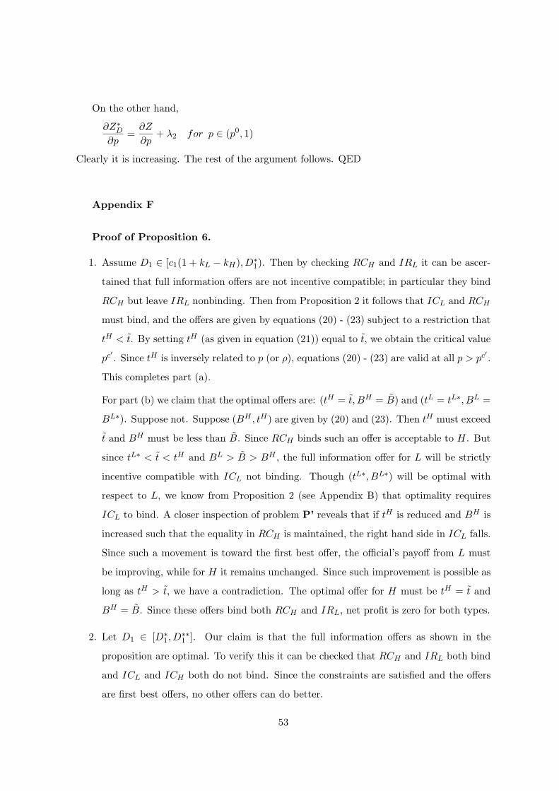
On the other hand,

∂Z∗D∂p

=∂Z

∂p+ λ2 for p ∈ (p0, 1)

Clearly it is increasing. The rest of the argument follows. QED

Appendix F

Proof of Proposition 6.

1. Assume D1 ∈ [c1(1 + kL − kH), D∗1). Then by checking RCH and IRL it can be ascer-

tained that full information offers are not incentive compatible; in particular they bind

RCH but leave IRL nonbinding. Then from Proposition 2 it follows that ICL and RCH

must bind, and the offers are given by equations (20) - (23) subject to a restriction that

tH < t. By setting tH (as given in equation (21)) equal to t, we obtain the critical value

pc′. Since tH is inversely related to p (or ρ), equations (20) - (23) are valid at all p > pc

′.

This completes part (a).

For part (b) we claim that the optimal offers are: (tH = t, BH = B) and (tL = tL∗, BL =

BL∗). Suppose not. Suppose (BH , tH) are given by (20) and (23). Then tH must exceed

t and BH must be less than B. Since RCH binds such an offer is acceptable to H. But

since tL∗ < t < tH and BL > B > BH , the full information offer for L will be strictly

incentive compatible with ICL not binding. Though (tL∗, BL∗) will be optimal with

respect to L, we know from Proposition 2 (see Appendix B) that optimality requires

ICL to bind. A closer inspection of problem P’ reveals that if tH is reduced and BH is

increased such that the equality in RCH is maintained, the right hand side in ICL falls.

Since such a movement is toward the first best offer, the official’s payoff from L must

be improving, while for H it remains unchanged. Since such improvement is possible as

long as tH > t, we have a contradiction. The optimal offer for H must be tH = t and

BH = B. Since these offers bind both RCH and IRL, net profit is zero for both types.

2. Let D1 ∈ [D∗1, D∗∗1 ]. Our claim is that the full information offers as shown in the

proposition are optimal. To verify this it can be checked that RCH and IRL both bind

and ICL and ICH both do not bind. Since the constraints are satisfied and the offers

are first best offers, no other offers can do better.

53

3. Suppose D1 ∈ (D∗∗1 , c1kLkH

]. It can be shown that full information offers bind IRL but

leave RCH nonbinding. Therefore, H will have incentive to misrepresent, which was

the case under strategy R. Then by adapting the arguments given in the proof of

Proposition 1 (see Appendix A) we can claim that ICH and IRL will bind, and optimal

tH and tL will be given by equations (12) and (14) respectively. Optimal BH is given

by ICH and optimal BL is given by IRL which are shown as BH and BL. These offers

must observe a restriction that tL > t. By setting tL (as given in equation (14)) equal

to t, we obtain the critical value pc′′. Since tL is also inversely related to p (or ρ),

these offers are valid if p < pc′′. This completes the proof of part (a). The proof of the

remaining part is analogous to the first case.

4. When D1 ∈ (c1kLkH, c1], the IRL curve will be strictly below RCH . By the logic used in

Proposition 1, only IRL and ICH will bind as in part (3.a). The rest follows.

QED

References

Balmohandas, V., Prabhakara Rao, J. V. and Hrushikesava Rao, P., 1991. Rural Banks

and Rural Credit. Discovery Publishing House, New Delhi.

Banerjee, Abhijit, 1997. A theory of misgovernance. Quarterly Journal of Economics

112(4): 1289-1332.

Chaudhuri, Sarbajit, and Gupta, Manas R., 1996. Delayed formal credit and the informal

credit market in agriculture: A theoretical analysis. Journal of Development Economics 51(2):

433-449.

Choi, Jay, P., and Thum, Marcel, 2003. The dynamics of corruption with the ratchet

effect. Journal of Public Economics 87: 427-443.

Dreze, Jean, 1990. Poverty in India and the IRDP delusion. Economic and Political

Weekly 25 (39): A95-104.

Ehrlich, Isaac, and Lui, Francis, T., 1999. Bureaucratic corruption and endogenous

growth. Journal of Political Economy 107 (December): S270-293

54

Government of India. 1998. Economic Survey 1997-98. New Delhi.

Gupta, Sanjeev, Davoodi, Hamid, and Tiongson, Erwin, 2001. Corruption and the provi-

sion of health care and education services, in Arvind K. Jain (ed.) The Political Economy of

Corruption, Routledge, London.

Hindriks, J., M. Keen and A. Muthoo, 1999. Corruption, extortion and evasion. Journal

of Public Economics, 74: 395-430.

Hoff, Karla and Stiglitz, Joseph E., 1990. Introduction: Imperfect information and rural

credit markets - puzzles and policy perspectives. The World Bank Economic Review 4(3):

235-250.

Jodhka, Surinder S., 1995. Bureaucratization, corruption and depoliticization: Changing

profile of credit co-operatives in rural Haryana. Economic and Political Weekly 30(1): 53-56.

Lewis, Tracy R., Sappington, David E., 1989. Countervailing incentives in agency prob-

lems. Journal of Economic Theory 49: 294-313.

Lui, Francis T., 1985. An equilibrium queuing model of bribery. Journal of Political

Economy 93(4): 760-781.

Maggi, G., Rodriguez-Clare, A., 1995. On countervailing incentives. Journal of Economic

Theory 66:238-265.

Marjit, Sugata, Mukherjee, Vivekananda and Mukherjee, Arijit, 2000. Harassment, cor-

ruption and tax policy. European Journal of Political Economy 16(1):75-94.

Mishra, Ajit, 2002. Hierarchies, incentives and collusion in a model of enforcement. Jour-

nal of Economic Behavior and Organization 47:165-178.

Reserve Bank of India, 2003, Handbook of Statistics on the Indian Economy, Reserve

Bank of India, Mumbai.

Rose-Ackerman, Susan, 1999. Corruption and Government: Causes, Consequences and

Reform. New York: Cambridge University Press.

Saha, Bibhas, 2001. Red tape, incentive bribe and the provision of subsidy. Journal of

Development Economics 65(2001): 113-133.

Saha, Bibhas, 2003. Harassment, corruption and tax policy: A comment on Marjit,

Mukherjee and Mukherjee, European Journal of Political Economy 19: 893-897.

Sarap, Kailas, 1991. Interlinked Agrarian Markets in Rural India. Sage Publications India

Ltd, New Delhi.

55

Shleifer, A., Vishny, R. W., 1993. Corruption. Quarterly Journal of Economics 108:

599-617.

World Bank, 1997. World Development Report 1997: The State in a Changing World.

Oxford University Press, New York.

56

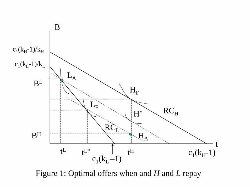
tHtL*tL

B

c1(kH-1)/kH

c1(kL-1)/kL

BL

BH

LF

HA

HF

LA

c1(kL –1)c1(kH-1)

t

Figure 1: Optimal offers when and H and L repay

RCH

RCL

H’

B

RCH

IRL

LF

HF

LA

HA

tHtH*tL*

BL

BH

tc1(kH-1) (c1-D1)kL

Figure 2: Optimal offers when L defaults

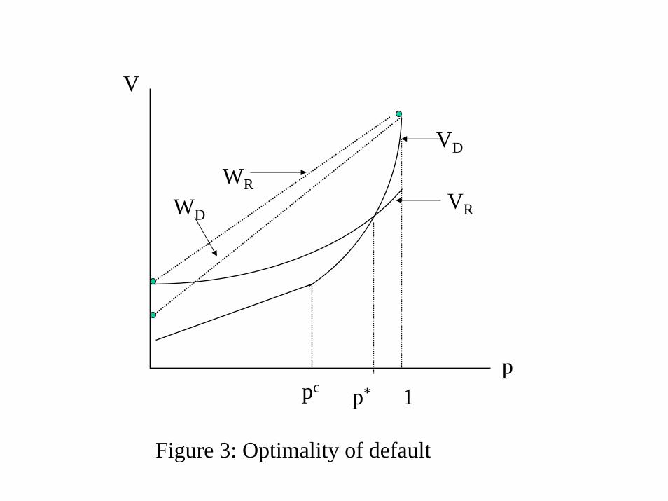
V

VD

WR

WDVR

ppc p* 1

Figure 3: Optimality of default

c1

_c1(c2)

p1

c*1(p) 1c~ (p)c1

++

c0

0 pµ p+p0

Figure 4: Optimal c1 for repayment

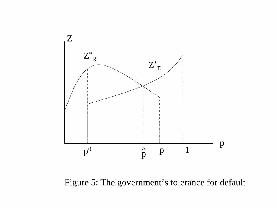
Z

p0 p+ 1

Z*R

Z*D

pp

Figure 5: The government’s tolerance for default

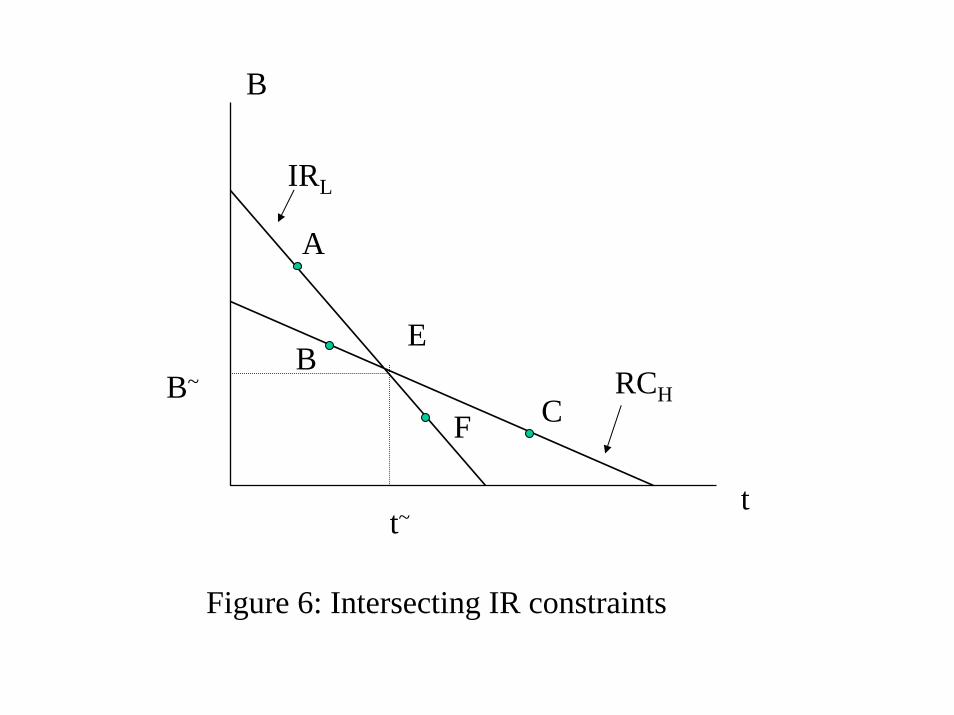
B

EB

A

IRL

CFRCHB~

tt~

Figure 6: Intersecting IR constraints

t

t~

D1* D1

**

tHA

tH*

tL*

tLA D1

c1kL/kH

Regime 3Regime 1

Regime 2

Figure 7: Different incentive regimes

t

tH

t~

tHA

tH*

tL*

tLA tL

D1D1

~D1*D1

^ D1**

Figure 8: Red tape and penalty on default

π1

π1L π1

H

D1**D1

*

D1D1

~D1^ c1

Figure 9: Information rents