Bi-Level Integrated System Synthesis (BLISS) - NASA · BI-LEVEL INTEGRATED SYSTEM SYNTHESIS (BLISS)...

NASA/TM-1998-208715

Bi-Level Integrated System Synthesis

(BLISS)

Jaroslaw Sobieszczanski-Sobieski

Langley Research Center, Hampton, Virginia

Jeremy S. Agte and Robert R. Sandusky, Jr.

The George Washington University

Joint Institute for Advancement of Flight Sciences

Langley Research Center, Hampton, Virginia

National Aeronautics and

Space Administration

Langley Research CenterHampton, Virginia 23681-2199

August 1998

https://ntrs.nasa.gov/search.jsp?R=19980234657 2019-07-22T12:00:19+00:00Z

Acknowledgments

The authors gratefully acknowledge the contributions of Dr. Srinivas Kodiyalam of the

Engineous Co. for providing test results for the Aircraft Optimization and the Electronic Package

Optimization using a software package called iSIGHT.

I The use of trademarks or names of manufacturers in this report is for accurate reporting and does not constitute an Iofficial endorsement, either expressed or implied, of such products or manufacturers by the National Aeronautics and I

Space Administration. ]

Available from the following:

NASA Center for AeroSpace Information (CASI)7121 Standard Drive

Hanover, MD 21076-1320

(301) 621-0390

National Technical Information Service (NTIS)

5285 Port Royal Road

Springfield, VA 22161-2171(703) 487-4650

BI-LEVEL INTEGRATED SYSTEM SYNTHESIS (BLISS)

Jaroslaw Sobieszczanski-Sobieski*, Jeremy S. Agte*,

and Robert R. Sandusky, Jr*

Abstract

BLISS is a method for optimization of engineering

systems by decomposition. It separates the systemlevel optimization, having a relatively small number of

design variables, from the potentially numerous sub-

system optimizations that may each have a large num-

ber of local design variables. The subsystem optimiza-

tions are autonomous and may be conducted concur-

rently. Subsystem and system optimizations alternate,

linked by sensitivity data, producing a design im-

provement in each iteration. Starting from a best guess

initial design, the method improves that design in it-

erative cycles, each cycle comprised of two steps. In

step one, the system level variables are frozen and the

improvement is achieved by separate, concurrent, and

autonomous optimizations in the local variable subdo-

mains. In step two, further improvement is sought in

the space of the system level variables. Optimum sen-

sitivity data link the second step to the first. The

method prototype was implemented using MATLABand iSIGHT programming software and tested on a

simplified, conceptual level supersonic business jet

design, and a detailed design of an electronic device.

Satisfactory convergence and favorable agreement withthe benchmark results were observed. Modularity of

the method is intended to fit the human organization

and map well on the computing technology of concur-

rent processing.

O. Introduction

Optimization of complicated engineering systems by

decomposition is motivated by the obvious need to dis-

* Manager, Computational AeroSciences, and Multi-

disciplinary Research Coordinator, NASA LangleyResearch Center, MS 139 Hampton VA 23681, AIAAFellow

* Graduate Research Scholar Assistant, George Washing-

ton University, Joint Institute for Advancement of Flight

Sciences, LT, United States Air Force

Professor, George Washington University, Joint Insti-tute for Advancement of Flight Sciences, AIAA Fellow

tribute the work over many people and computers toenable simultaneous, multidisciplinary optimization. It

is important to partition the large undertaking intosubtasks, each small enough to be easily understood

and controlled by people responsible for it. This im-

plies granting people in charge of a subtask a measure

of authority and autonomy in the subtask execution,

and allowing human intervention in the entire optimi-

zation process.

Reconciliation of the need for subtask autonomy with

the system level challenge of "everything influences

everything else" is difficult. Each of the leading MDO

methods that have evolved to date (survey papers:

Balling and Sobieszczanski-Sobieski, 1996; and Sobi-eszczanski-Sobieski, J., and Haftka, R. T, 1997) tries to

address that difficulty in a different way. In the system

optimization based on the Global Sensitivity Equations

(GSE) (Sobieszczanski-Sobieski, J. 1990, Olds, J.1992, Oids, J. 1994), the partitioning applies only in

the sensitivity analysis while optimization involves all

the design variables simultaneously. The Concurrent

SubSpace Optimization method provides for separate

optimizations within the modules (Sobieszczanski-Sobieski, J. 1988, Renaud and Gabriele, 1991, 1993,

and 1994; Stelmack and S. Batill, 1998) but handles all

the design variables simultaneously in the coordination

problem. The Collaborative Optimization method

(Braun and Kroo, 1996; Sobieski and Kroo, 1998) also

enables separate optimizations within the modules,

each performed to minimize a difference between the

state and design variables and their target values set in

a coordination problem. This problem combines the

system optimization with the system analysis, therefore

its dimensionality may be quite large.

Most of the above method implementations had to

overcome difficulties with integration of dissimilarcodes. This has stimulated use of Neural Nets and Re-

sponse Surfaces as means by which subdomains in thedesign space may be explored off-line and still be rep-

resented to the entire system. Unfortunately, effective-

ness of this approach is limited to approximately 12 to

20 independent variables, hence, it is best suited for the

early design phase. Consequently, a clear need remains

National Aeronautics and Space Administration

1

for a method applicable in later design phases when

the number of design variables is much larger. Meth-

ods that build a path in design space fit that require-

ment. Ultimately, one needs both domain-exploringmethods and path-building methods, enhanced with

seamless 'gear-shifting' between the two.

Motivated by the above state of affairs, BLISS attacks

the problem by performing an explicit system behaviorand sensitivity analysis using the GSE, autonomous

optimizations within the subsystems performed to

minimize each module contribution to the system ob-jective under the local constraints, and a coordination

problem that engages only a relatively small number of

the design variables that are shared by the modules.

Solution of the coordination problem is guided by the

derivatives of the behavior and local design variables

with respect to the shared design variables. These de-

rivatives may be computed in two different ways, giv-ing rise to two versions of BLISS.

In either version, BLISS builds a gradient-guided path,

alternating between the set of disjointed, modular de-

sign subspaces and the common system-level design

space. Each segment of that path results in an im-proved design so that if one starts from a feasible state,

the feasibility in each modular design subspace is pre-served while the system objective is reduced. In case ofan infeasible start, the constraint violations are reduced

while the increase of the objective is minimized. Be-

cause the system analysis is performed at the outset of

each segment of the path, the process can be termi-

nated at any time, if the budget and time limitations so

require, with the useful information validated by the

last system analysis. In addition to enabling complete

human control in the subspace optimization, BLISS

allows the engineering team to exercise judgment, at

any point in the procedure, to intervene before com-mitting to the next successive pass.

BLISS has been developed in a prototype form and hasbeen successfully demonstrated on the small-scale test

cases reported herein.

1. Notation

BB - black box, a module, in the mathematical model

of a system.

BBA(Yr,(Z,Xr)) - analysis of BBr to compute Y_ forgiven Z and Xr

BBOFr- BB Objective Function computed in BBr

BBOPTr(Xr,_r, Gr) - optimization in BB_ defined byeq.(2.1/9)

BBOSA_(X_.opt,Z,Y_.s) - analysis of BB optimum for

sensitivity to parameters

BBSA(D(Yr,(Z,Xr,Yr.0) - sensitivity analysis of BB_ to

compute its output derivatives w.r.t. Z, X_, and Y_._D(V1,V2) - total derivative dVl/dV2

d(VI,V2) - partial derivative OVI/OV2;

D0, and d0 dimensionality depends on the dimen-sionalities of V1 and V2:

V1 and V2 - are both scalars, then D and d arescalars

V 1 vector, V2 scalar, then D and d are vectors

V 1 scalar, V2 vector, then D and d are vectors

V1 vector, V2 vector, then D and R are matrices

Go - vector of constraints active at the constrained

minimum, length NGo

Gr - vector of the constraint functions, gr.t local to BB_,gr,t -<0 is a satisfied constraint

Gyz - constraints in a BB that have a stronger dependence on Y and Z, than on X

GSE - Global Sensitivity Equations (Sobieszczanski-

Sobieski, 1990); GSE/OS - GSE/Optimized Sub-systems.

I - identity matrix.

L - vector of the Lagrange multipliers corresponding toGo, length NGo

LP - Linear Programming

NB - the number of BBs in the system

NLP - NonLinear Programming

opt - subscript denotes optimized quantity

P - vector of parameters, Pi, kept constant in the proc-

ess of finding the constrained minimum, lengthNP.

SA((P,Z,X),Y) - system analysis; a computation that

outputs Y for a system defined by P, Z, and X

SOF - System Objective Function computed in one ofthe BBs

SOPT(Z,O) - system objective optimization defined byeq. (2.2.3/1)

SSA(D(Y,(Z,X)) - system sensitivity analysis to com-pute sensitivity of the system response Y w.r.t. Zand X

TOGW - take-off gross weight

T - superscript denotes transposition.

Xr - vector of the design variables xr,j, length NXr,these variables are local to BBr; X without sub-

script - a vector of all concatenated Xr, length NXXL, XU - lower and upper bounds on X, side-

con straints.

Yr - vector of behavior (state) variables output fromBBr, these are the coupling variables; an element

of Yr is denoted Yr,i; some of Y_.iare routed as in-

puts to other BBs, and may also be routed as out-

put to the outside; the Y_ length is NY_; Y without

subscripts - a vector of all concatenated Y_, lengthNY


2

Y,,s - vector of variables input to BBr from BBs, these

are the coupling variables; an element of Yr,_ is de-

noted Yr,s.i; note that by this definition Yr._ is a sub-

set of Yr, vector length NYr._

Z - vector of the design variables Zk that are shared by

two or more BBs, these are the system-level vari-

ables; length NZ

0 - subscript denotes the present state from which to

extrapolate, or the optimal state.

ZL, ZU - lower and upper bounds on Z, side-constraints

A - increment

AZL, AZU - move limits

0r - the local objective function in BB_

- the system objective function equated to one, par-

ticular yj,i

2. The Algorithm

In this section, the symbols defined in Notation are

used in a shorthand manner without repeating their

definitions.

ztm 1

Y2,1 y_Y3.1 Iz

Figure 1: System of Coupled BBs

The algorithm is introduced using an example of a

generic system of three BBs, as shown in Figure 1.Three is a number small enough for easy conceptual

grasp and compact mathematics, yet large enough to

unfold patterns that readily generalize to larger NB.Even though the system in Figure 1 is generic, it may

be useful to bear a specific example in mind. Let it bean aircraft so that:

BB 1 - performance analysis

BB2 - aerodynamicsBB3 - structures

- maximum range for given mission characteristics

Yi.2 - includes the aerodynamic drag; Y1.3 - includes thestructural weight; Y2.1 - includes Mach number;

Y3.1 - includes TOGW; Y2.3 - includes the struc-tural deformations that alter the aerodynamic

shape; Y3.2 - includes the aerodynamic loads

gl.t - a noise abatement constraint on the mission pro-

file; g2.t - limit of the chordwise pressure gradient;

g3.t - allowable stress

x_,j- cruise altitude; x2.j - leading edge radius; x3.j-sheet metal thickness in the wing skin panel No.138

zj - wing sweep angle; z2 - wing aspect ratio; z3 - wingairfoil maximum depth-to-chord ratio; z4 - loca-

tion of the engine on the wing

The system in Figure 1 is characterized by BB level

design variables X, and by system-level design vari-

ables Z. As a reference, if an all-in-one optimization

were performed, observing the system at a single level

and making no distinction between the treatment of X

variables and the treatment of Z variables, the problemcould be stated

Given: X and Z (1)

Find: AX and AZ

Minimize: _(X,Z,Y(X,Z))

Satisfy: G(X,Z,Y(X,Z)

Since BLISS approaches this optimization by means of

a system decomposition, the algorithm depends on the

availability of the derivatives of output with respect to

input for each BB. That assumes the differentiability ofthe BB internal relationships to at least the first order.

It is immaterial how the derivatives are computed, fi-

nite differencing may always be used, but it is expectedthat in most cases one will utilize one of the more effi-

cient analytical techniques (Adelman and Haftka,

1993).

The algorithm comprises the system analysis and sen-

sitivity analysis, local optimizations inside of the BBs(that includes the BB-internal analyses), and the sys-

tem optimization. We will not elaborate on SA beyond

pointing out that it is highly problem-dependent, andlikely to be iterative if there are any non-linearities in

the BB analyses. Each pass through the BLISS proce-

dure improves the design in two steps: first by concur-

rent optimizations of the BBs using the design vari-

ables X and holding Z constant; and next, by means of

a system-level optimization that utilizes variables Z.

We begin with the BB-levei optimization.

2.1. BB-level (discipline or subsystem)

optimizations.

The basis of the algorithm is the formulation of an

objective function unique for each BB such that mini-


3

mizationof thatfunctionin eachBBresultsin theminimizationof thesystemobjectivefunction.To in-troducethatformulationletusbeginwiththesystemobjectivefunction(SOF).TheSOFis computedasasingleoutputitemin oneof theBBs;withoutlossofgeneralityweassumethatit isBBIsothat

= Yl.i (1)

is one of the elements of Y1.

Total derivatives of Y w.r.t, xr.j, D(Y, xr,j), are com-

puted according to Sobieszczanski-Sobieski, 1990, by

solving a set of simultaneous, algebraic equations

known as Global Sensitivity Equations, GSE, (see Ap-

pendix, Section 1, for details) for a particular x_,j

[A] {D(Y,xr.j)} = {d(Y, Xr.j)} (2)

where A is a square matrix, NYxNY, composed ofsubmatrices forming this pattern

I A1, 2 Am,3]

A2,1 I A2,31

A3,1 A3,2 I

(3)

where I stands for identity matrix, NY_xNYr, and Ar.s

are matrices of the derivatives that capture sensitivityof the BBr output to input. For example

A2,3 = -[d(Y2,Y3)], NY2xNY3

A3.2 = -[d(Y3,Y2)], NY3xNY2 (4)

One should note that eq. 2 can be efficiently solved for

many different xr.j using techniques available for linearequations with many right-hand sides.

Having D(Y,xr.j) computed from eq. 2 for all Xr,j, wecan express _ as a function of X by the linear part ofthe Taylor series

t_ = Yl.i = (Yl,i)0 + D(yl.i, Xl )Tzkxl +

D(yl,i, x2)TAx2 q- D(yl.i, x3)T,_kX3 (5)

where D-terms are vectors of length NXr.

We see from eq. 5 that

A_ = D(yl.i,X1)TAX1 + D(yl,i,X2)TAX2 +

D(yl.i,x3)TAX3 (6)

the three terms showing explicitly the contributions

to AO of the local design variables from each of thethree BBs.

It is apparent that to minimize AO we need to charge

each BB with the task of minimizing its own objective.Using BB/ as an example, objective _2 is

(_2 ----"D(yl.i, x2)TAx2.j , j = 1--->NX2 (7)

The above equations state mathematically the fun-

damentally important concept that in a system op-

timization the contributing disciplines should not

optimize themselves for a traditional, discipline-

specific objective such as the minimum aerodynamic

drag or minimum structural weight. They should

optimize themselves for a "synthetic" objective

function that measures the influence of the BBr de-

sign variables Xr on the entire system objectivefunction.

Another way to look at it is to observe that, in long-hand

(_2_"D(yLi, x2,I)TAx2,1 -.bD(yl.i, x2,2)TAx2,2 -1-...

+ D(yLi, X2,j)T_kx2,j -l" .... j = I--->NX2 (8)

so it may be regarded as a composite objective function

commonly used in multiobjective optimization. One

may say, therefore, that in a coupled system the local

disciplinary or subsystem optimizations should be

multiobjective with a composite objective function. The

composite objective should be a sum of the local designvariables weighted by their influence on the single ob-

jective of the whole system. It should be emphasized

that this is true also in that particular BB, where O is

being computed. In the aircraft example it is • = Yl.i in

BBt according to eq. 1. However, the BBI optimization

objective is not ¢, = YLi. Instead, it is _ from an equa-tion analogous to eq.8.

The local optimization problem may be stated formallyfor BB2

Given: X2, Z, and Y2,1 , Y2,3 (9)

Find: AX2 ; length NX2

Minimize: 1_2 = D(yl,i,x2)TAx2

Satisfy: G2 < 0, including side-constraints

Incidentally, we adhere to the convention which calls

for minimization of the objective function. If the appli-


4

cationrequiresthatfunctionbemaximized,asit doesin theexampleof aircraftrange,weconverttheobjec-tive,e.g.,• =- (range).

TheoptimizationproblemforBB_,andBB3areanal-ogous.All threeproblemsbeingindependentof eachothermaybesolvedconcurrently.Thisis anopportu-nity for concurrentengineeringandparallelprocess-ing.

Bysolvingeq.9 forallthreeBBs,wehaveimproved-thesystembecause,accordingtoeq.5 and6,wehavereduced• byA_, whilesatisfyingconstraintsineachBB.

2.2. System-level optimization.

So far we have improved the system by manipulating X

in the presence of a constant Z. We can score further

improvement by exploiting Zs as variables. To do so

we need to know how Z influences • = Yl.i. That is, we

need D(yl.i,Z).

At this point, the BLISS algorithm forks into two al-ternatives, termed BLISS/A and BLISS/B.

2.2.1. BLISS/A

This version of BLISS computes the derivatives of Y

with respect to Z by modified GSE, eq.(2.1/2) (equa-tions from other sections are cited in 0, the section

number given before the/). The GSE modification ac-counts for the fact that optimization of a BB turns its X

into a function of Y and Z that enter that particular BB

as parameters. The modification leads to a new gener-alization of GSE that takes the following form

I_D(X, Zk)J [d(X, zk)J(1)

termed GSE/OS for GSE/Optimized Subsystems. The

GSE/OS yields a vector D(Y,Zk) and D(X,Zk), and be-cause • is one of the elements of Y, • = Yt.i, we get the

desired derivative D(O,Zk). Derivation and details of

the GSE/OS structure, including the definition of thematrix M, are in Section 2 of the Appendix. At this

point it will suffice to say that the matrix of coefficients

in GSE/OS is populated with d(Yr,Ys), d(Yr,Xr), and

d(Xr,Ys). These terms and the RHS terms of d(Y,Zk)

and d(X,Zk) are obtained from the following sources

• d(Yr,Y0, d(Y_,Xr), and d(Y,z0 ...... from BBSA• d(Xr,Zk), d(X_,Y0 ..................... from BBOSA

The terms d(X,Zk) and d(X_,Y0 are the derivatives of

optimum with respect to parameters that, in principle,

may be obtained by differentiation of the Kuhn-Tucker

conditions, e.g., an algorithm described in Sobieszc-

zanski-Sobieski et al, 1982. That approach, however,

requires second order derivatives of behavior, too

costly in most large-scale applications. Therefore, an

approximate algorithm adapted from Vanderplaats and

Cai, 1986, is given in Section 3 of the Appendix. In

that algorithm, parameters are perturbed by a smallincrement, one at a time, and the BB optimization is

repeated by Linear Programming (LP) starting from

the optimal point. Derivatives of optimal X and Y

with respect to parameters are then computed by finitedifferences.

2.2.2. BLISS/B

This version of BLISS avoids calculation of d(Xr,Zk)

and d(X_,Y0 altogether by using an algorithm that

yields D(_,P), where P includes both Y and Z. The

algorithm, described in literature (e.g., Barthelemy andSobieszczanski-Sobieski, 1983) is based on the well-

known notion that the Lagrange multipliers may be

interpreted as the prices, stated in the units of O, forthe constraint changes caused by incrementing p,. For a

general case of the objective F=F(P) and Go= Go(P), thealgorithm gives the following formula for D(F,P)o

D(F,P)o=d(F,P) + LTd(Go,P)

To use the above in BLISS, consider that in P we have

an independent Z but Y=Y(Z) so that the terms d0

require chain-differentiation. Hence, the above generalformula tranforms to

D(yl,i,Z)o T = (L r d(Go,Z))l + (LTd(Go,Z))2 +

(Lrd(Go,Z))3 + [(LXd(Go,Y))t+ (LTd(Go,Y))2

+ (LTd(Go,Y))3 ](D(Y,Z)) + D(yLi,Z) T (1)

where L is the vector of Lagrange multipliers and ( )_,

( )2, and ( )3 identify the BBs 1, 2, and 3.

The terms in the above equation originate from the

following sources:

• d(Go,Z) and d(Go,Y) - BBSA performed on iso-

lated BB_

• L - obtained for BBr at the end of BBOPT

• D(Y,Z) - from GSE in SSA

• D(y_.i ,Z) - the column corresponding to yl.i in the

above matrix D(Y,Z)


5

BLISS/Bis substantiallysimplerin implementationthan BLISS/A and it eliminates the computational cost

of one LP per parameter Y and Z. Optimizers that yieldL as a by-product of optimization are available for use

in BBOPT, or L may be obtained as described inHaftka and Gurdal, 1992.

2.2.3. Optimization in the Z-space.

Once D(y].i,Z) have been computed from either

eq.(2.2.1/1) or as D(yl.i,Z)o from eq. (2.2.2/1), we can

further improve the system objective by executing thefollowing optimization, using any suitable optimizer

Given: Z and O0 (1)

Find: AZ

Minimize: • = O0 + D(yl.i,Z)TAZ

Satisfy: ZL < Z + AZ < ZU; AZL < AZ < AZU

Where _0 is inherited from the previous cycle SA for

X and Z (initialized if it is the first cycle). It is rec-

ommended to handle the Z constraints by means of atrust-region technique, e.g., Alexandrov 1996. In the

above, term D(yLi , Z) is a constrained derivative that

protects Go = 0 in all BBs. Therefore, the optimizationis unconstrained except of the side-constraints andmove limits.

However, some BBs may have constraints that depend

on Z and Y more strongly than on X (in the extreme

case some constraints may not be functions of X at all,

only of Y and Z). Such constraints, denoted Gyz, maybe difficult (or impossible) to satisfy by manipulating

only X in BBOPT. To satisfy them, one must add to the

Z-space optimization in eq. 1 their extrapolated values

GyzT = Gyz.OT + (d(Gyz,Z) +

d(Gyz,Y)D(Y,Z))TAZ < 0 (2)

where d(Gyz,Z), and d(Gyz,Y) are obtained from BBSA.In this instance, the Z-space optimization becomes aconstrained one.

3. Iterative Procedure

The two operations, the local optimizations in the BBsand the system-level optimization, described in Sec. 2,

result in a new system, altered because of the incre-

ments on X and Z. This means that inputs to and out-puts from SA, BBA, BBSA, SSA, BBOPT, BBOSA

(BLISS/A), and SOPT all need to be updated, and the

sequence of these operations repeated with the new

values of all quantities involved, including new values

of all the derivatives because they would change if

there were any nonlinearities in the system (as thereusually are).

In a large-scale application where execution of each

BLISS cycle may require significant resources and

time, the engineering team may wish to review the

results before committing to the next cycle. That inter-

vention may entail a problem reformulation, such as

overriding the variable values, deleting and addingvariables, constraints, and even BBs.

t

SA • X=Xo+ AXomtmlUallm X & Z

I Z=Zo+ AZ_

f eq. {AI-A6)

STOP 1 EVALUATE IcPJrRRIA

t'¢l. (AI'A6) d,( * II_ eq. (AI-A6)¥ T

BBSA [ BBSABBj BB/

d(Y,,XJ d(Yj,Xj)

d(G_,Ytj) SSA d(GI,Yjj)

d( Gi, Z) eq. (2.1/2) d(GpZ)

,#

BBI BB l

tq. _2.1/9_ _ eq. (2.1/9)

AXoM

D(_ ,_eq. (2A,2_)

1SOPTeq. g2.2._ ,2 )

AZm,T

UPDATE J X=Xo+AX _VARIABLES Z=Zo+ AZo_

Figure 2: BLISS/B Flowchart

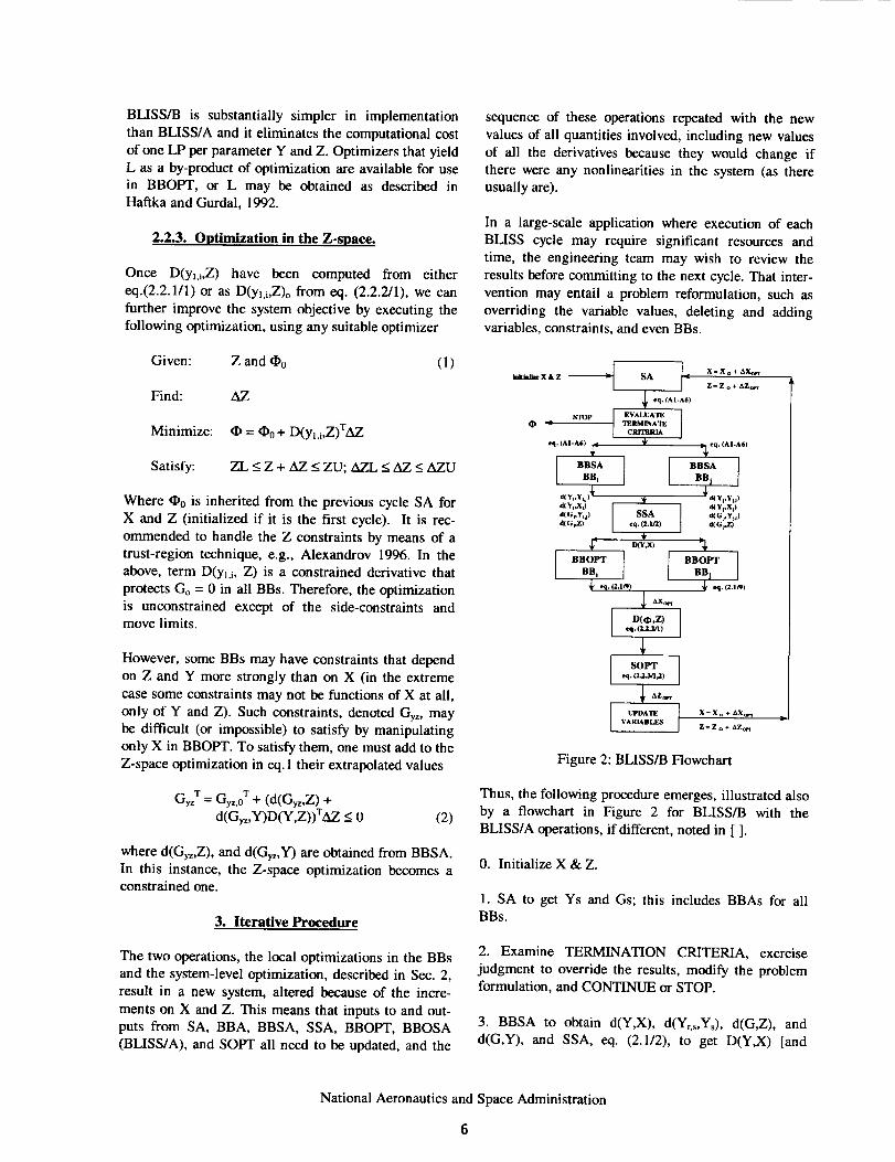
Thus, the following procedure emerges, illustrated also

by a flowchart in Figure 2 for BLISS/B with the

BLISS/A operations, if different, noted in [ ].

0. Initialize X & Z.

1. SA to get Ys and Gs; this includes BBAs for allBBs.

2. Examine TERMINATION CRITERIA, exercise

judgment to override the results, modify the problemformulation, and CONTINUE or STOP.

3. BBSA to obtain d(Y,X), d(Yr.s,Y_), d(G,Z), and

d(G,Y), and SSA, eq. (2.1/2), to get D(Y,X) land


6

D(Y,Z)];Here is an opportunity for concurrent process-

ing.

4. BBOPT for all BBs, eq. (2.1/9) using

formulatedindividually for each BB (eq. (2.1/6, 7)),

get Coot and AXopt; obtain L for Go [skip L]. Here is an

opportunity for concurrent processing.

5. Obtain D(C,,Z) as in eq. (2.2.2/1). [Execute BBOSA

to obtain d(X,Z) and d(X,Y), and form and solve

GSE/OS (Appendix, Section 3) to generate D(Y,Z)].

Here is an opportunity for concurrent processing.

6. SOPT to get AZopt by eq. (2.2.3/1 and 2) herein.

7. Update all quantities, and repeat from 1.

X : X 0 + AXopt; Z = Z -4- Z_Zop t

Note: Termination is placed as #2 after SA to ensure

that the full analysis results document the final system

design, as opposed to having it documented only by the

extrapolated quantities. Also, at this point the engi-

neering team may decide whether to intervene by

modifying the variable values, and adding or deleting

the design variables and constraints.

When started from a feasible design, the procedure will

result in an improved system, while the local con-

straints are kept satisfied within extrapolation accu-

racy, even when terminated before convergence.

Figure 3: Polynomial Representation of Wing Twist

In case of an infeasible design start, the improvementwill be in the sense of reductions in the constraint vio-

lations, while the objective may exhibit an increase, at

least initially. The procedure achieves the improvement

by virtue of optimization alternating between the do-

main of NB X-spaces (Step #4) and the single Z-space

(Step #6).

Caveat: because in BLISS/B the extrapolation of • in

eq. (2.2.3/1) is based on the Lagrange multipliers in

eq. (2.2.2/1), its accuracy depends on the BBOPTyielding a feasible solution, and on the active con-

straints Go remaining active for updated Z. If someconstraints leave the active set Go, or new constraints

enter, a discontinuous change of the extrapolation error

may result. For example, consider the wing aspect ratio

AR as a Z-variable and suppose that for AR = 3 it is

the stress due to the wing bending that is one of the

active constraints in the structures BB. If optimization

in the Z-space took the design to AR = 4, the next cy-

cle may reveal that the stress constraint is satisfied but

a flutter constraint becomes critical. Past experience

(Sobieszczanski-Sobieski, 1983) shows that this dis-

continuity is likely to slow, but not to prevent, the pro-

cess convergence, and may be controlled by adjustingthe move limits.

t/c, h, M, AR, A, S_

Structures _,

AR aspect ratio

C_kin frier, coef.

D -drag

ESF-eng. scale fact.

h-altitude

L lift

M Mach g

Nz-max_ load fact.

R range

SFC-spec, fuel cons.

SILEF-wmg surf, areaT throttle

ffC thickness/chord

WaE-baseline eng. wt,

WE-engine weight

WF-fuel weight

W_o-misc. fuelwt

Wo-misc. weight

WT-totat W eight

x-w ingbox x-sect

A wing sweep

_.-tlperratio

Figure 4: Data Dependencies for Range Optimization

4. Numerical Tests and Examples

BLISS/A was tested on a sample of test problems from

Hock and Schittkowski, 1981, and on a design of an

electronic package. BLISS/B was exercised on the lat-

ter, and also on a very simplified aircraft configuration

problem. Both versions of BLISS performed as in-

tended in all of the tests. The sole purpose of these

initial numerical experiments was to test and to dem-onstrate the BLISS procedure logic and data flow,

therefore, the BBs were merely surrogates of the nu-

merical processes that need to be used in real applica-tions.


7

4.1. Aircraft Optimization

The aircraft test was an optimum cruise segment of a

supersonic business jet based on the 1995-96 AIAA

Student Competition. This problem was selected be-

cause of its available data base and the availability of 'the black boxes written in Visual Basic in form of Ex-

cel spreadsheets. The supersonic business jet was mod-

eled as a coupled system of structures (BB0, aerody-

namics (BB2), propulsion (BB3), and aircraft range

(BB4). All the disciplines were represented by modules

comprising an analysis level typical for an early con-ceptual design stage.

var \ cycle* 1 2 3 4 5

Range(SSA) 535.79 1581.67 3425.35 3961.41 3963.9E

ExtpI. Error -535.79 -536.67 -431.63 -56.26 -3.4

BB1 ExtpI. 17.17 -0.16 -3.26 -0.86 0.0(

BB2 Extpl. 1 6.85 0.00 0.00 0.00 0.0,

BB3 Extpl. 26.00 110.92 -76.84 0.00 0.0_

X Extpl. 60.02 110.75 -80.10 -0.86 0.0¢

Z Extpl. 449.19 1301.30 559.90 0.00 0.0¢

Range(Extpl.) 1045.00 2993.72 3905.15 3960.56 3963.91]

_. 0.25 0.14951 0.17476 0.25775 0.38757

x 1 0.75 0.75 0.75 0.75

Cf 1 0.75 0.75 0.75 0.71

T 0.5 0.1676 0.20703 0.15624 0.15624

tic 0.05 0.06 0.06 0.06 0.06

h(ft) 45000 54000 60000 60000 60000

M 1.6 1.4 1.4 1.4 1.4

AR 5.5 4.4 3.3 2.5 2.5

A(*) 55 66 70 70 70

Sn,f(ft=) 1000 1200 1400 1500 1500

*One cycle is one pass through the BLISS procedure

Table 1: A/C Results for 20% Move Limit

The aircraft optimization was a maximization of ther-

ange computed through the Breguet range equation.

For testing purposes, additional design and state vari-

ables were introduced in BBs 1 through 3, and func-

tional relationships not present in the original BBs

were supplied to reflect what is commonly known

about the typical functions involved in design. For ex-

ample, stress is expected to fall as a reciprocal of the

increase of the skin thickness in a wing box. Such re-lationships were represented by polynomial functions.

One plot of such a function is shown in Figure 3, por-

traying the wing twist as a function of the wing box

cross-sectional dimensions scale factor and the winglift.

Section 4 of the Appendix defines the BBs in this ex

ample by their input and output variables, and by the

functions that link output to input. Table A1 also iden-tifies local constraints and side constraints. Note that

BB2 contains a constraint that does not depend on its X

or Y input, thus the Z-space optimization is a con-

strained one, per eq. (2.2.3/1 & 2). Side constraints on

Z were judiciously selected to guard against conditions

not accounted for in the BBAs. For example, the lowerbound of 2.5 on aspect ratio stemmed from the sub-

sonic performance considerations.

hum _ den _. x C_ T t/¢

Wr 0.01146 1.71536 0.01981 -0.15744 0.12714

W_ 0 0 0 0 0.72626

O -0.03342 0.19971 3.31E-15 -1.73E-14 -2.10E-14

L 0.01146 1.71536 0.01981 -0.15744 0.12714

B -4.19E-05 0.00581 0.12457 -0.00049 0.68108

L/D 0.0115 i 1.7095 -0.1046 -0.15694 -0.54935SFC 1.98E-20 -5.07E-18 -2.70E-17 0.08544 0

WE -4.40E-05 0.0061 0.13083 -1.03986 0.71531

ESF -4.19E-05 0.00581 0.12457 -0.99059 0.68108

R -0.00077 -0.12692 -0.12581 -0.07299 0.10115

num _ den h M AR Sweep Sr_

Wr -0.33931 0.31956 0.08208 0.2537 0.55182

W_ 0 0 -0.36043 0 1.09211

O -1.93E-13 -6.15E-t4 -0.10766 3.77E-14 -0.10766

L -0.33931 0.31958 0.08208 0.2537 0.55182

D -2.1339 2.00984 3.37E-06 -0.83983 0.99838

LID 1.84108 -1.6507 0.08207 1.10064 -0.43675

SFC 0.12946 0.05555 2.31E-17 -1.86E-16 0

WE -2.24115 2.11086 3.54E-06 -0.88204 1.04857

ESF -2.1339 2.00984 3.37E-06 -0.83983 0.99838

R 2.07616 -1D4784 -0.39618 0.82904 0.15535

Table 2: Normalized Y Derivatives w.r.t. X and Z

The BBs are coupled by the output-to-input data

transfers (design structure matrix) depicted in Figure 4.

Note that BB4 is an analysis-only module and does notfeedback any data to other BBs.

4000

3S00

3000

_ 2500

1

0E_ 1500

to

1000

500

............................... ._......_J......../_ ..............!

/

' /. . _yatem O I_e_li_te_,' k ./. .....

//'

.... . ......... .... /J

..... i• _- Exl_pOIIt lion Ell'or

i _ '-6002 4 5

Cycle Number

Figure 5: Range and Extrapolation Error Histogram

This test was conducted entirely using MATLAB 5 andits Optimization Toolbox. The entire MATLAB code

listing for the aircraft range model may be found in

Section 5 of the Appendix. To establish a benchmark,

the system was first optimized using an all-in-one ap-

proach in which the MATLAB optimizer was coupleddirectly to SA and saw no distinction between the X

and Z variables. Next, the test case was executed using

86

z-171 .E

-257_

o

-343 ._

-429 _x

-514


8

BLISS/B, starting at different infeasible initial points

chosen by varying the six design variables that are not

arguments in the polynomial functions. The choice of

initial values for variables that are arguments of the

polynomial functions was limited due to the nature of

the polynomial formulation. This limitation is not acharacteristic of the BLISS method itself, as the poly-

nomial functions would not be required in a large scale

optimization problem. With the move limits ranging

from 10 to 70 %, the procedure convergence was sat-

isfactory through the move limits of 60% for all initial

points tested. However, in nearly all cases, no addi-

tional improvement in convergence rate was recorded

for move limits greater than 20%. For instance, the

objective function was advanced to within 1% of the

benchmark in 5 passes for move limits 20 and 30%.Onset of an erratic behavior was observed with move

limits increased past 60%, the procedure converged or

diverged dependent on the starting point.

h

X-sect G Throttle

HAR

M

Design Variables

Figure 6: Range Sensitivities (1 st cycle)

Table 1 displays a sample of typical results for themove limits value of 20%. It shows that the initial de-

sign range was extremely poor, only 536 nm. BLISS/B

improvements advanced the range to 3964 nm. The

range converged monotonically, although in some

cases small amplitude oscillations were observed.

Comparison of the extrapolated and actual values of

the objective and constraints shows reasonable accu-

racy and conservatism of the extrapolations. The opti-mal values of the design variables reflect numerous

tradeoffs typical for aircraft design. For instance, opti-mal t/c resulted, in part, from a trade-off between the

wave drag and structural weight. Table 2 shows nor-

malized (logarithmic) derivatives of all Ys , including

the range, w.r.t, all the X and Z variables, sampled in

Cycle 1 to illustrate sensitivity of the system solution todesign variables.

Figure 5 illustrates the range histogram, and depicts

the extrapolation error as being effectively controlled

by the move limits. Range sensitivities to X and Zvariables are shown in Figure 6. As expected, altitude

and Mach number have the largest effect on the objec-

tive function, while taper ratio has the smallest.

1400

/ ': [ BB10bi (2'1/7j

12001- ........ ' ..... I .... BB2 CIbI (2.1t71

I : | .... B B30bi (:Z.'_,'71

= _. _ ,,,oh <222,,,)

1000 ..... . - :..... .. ..... --_

e_ 80oi -. .,....... ......... :........ :

# .' : , !soo_........ _.......... ...... _...........

_o L'/

,,oo............ i .............. i :: ..... i ..........

o_=-" ' " _. ""' _ .... :

1 2 3 4

Cycle Ntlm bar

Figure 7: BB and System Contributions to Range

Figure 7 shows the individual BB and system contri-

butions to the range objective in each cycle. Here it isobserved that, in this particular case, the contribution

of system level variables is significantly larger thanthat of the local variables in the extrapolation of range.

This test case was also implemented in a software

package for system analysis and optimization callediSIGHT (iSIGHT, 1998). The iSIGHT and MATLAB

results cross-check was completely satisfactory.

4.2 Electronic Package optimization

The electronic packaging was introduced as an MDO

problem in Renaud, 1993. Its electrical and thermal

subsystems are coupled because component resistanceis influenced by operating temperatures and the tem-

peratures depend on resistance.

The objective of the problem is to maximize the watt

density for the electronic package subject to con-

straints. The constraints require the operation tem-

peratures for the resistors to be below a threshold tem-

perature and the current through the two resistors to be

equal. The system diagram in Figure 8 shows the data

dependencies for two BBs, representing electrical re-

sistance analysis and thermal analysis. As Figure 8indicates, there are no "natural" Z's in this case.

Therefore, Z's were created as targets imposed on each


9

of theY's andtheBBOPT'swererequired to match

the Y values to those Z targets (similar as it is done inthe Collaborative Optimization method). Details of the

electronic packaging problem may be found in Padula,1996.

(X],X2, X3,X,) (X_,X6,XT, Xs)

(t'2,1"_)

,Temperature

Electrical I

Figure 8: Electronic Packaging Data Dependencies

This test case was implemented in iSIGHT using

BLISS/A and B. A benchmark result was obtained by

executing an all-in-one optimization from various

starting points ("A-in-O" column). BLISS/A and B

were started from the same points. Table 4 displays the

benchmark and the BLISS/A and B results as showing

a good agreement. Table 4 also indicates a comparisonof the computational labor (the "Work" column) meas-

ured by the number of BB evaluations necessary toconverge the fixed-point iterations in BBAs and in SA,

all repeated as needed to compute derivatives by finite-

differences in a gradient-guided optimization. As Table

4 shows, the BLISS/B computational labor was sub-

stantially lower than the benchmark in all cases.

Method Cale

A-in-O 1

2

34

BLISS/A 12

34

BLISS/B 1

2

3

4

Initial DeBign IniL _ Ma= Final Design Fin. Des. MaxObjective Constr. Vlol. Objlctivo Conltr. Viol.

7.79440E+01 2.16630E-08 6.39720F+05 1.22E-0:6.83630E+03 -2.89560E-01 6.39720E+05 1.22E-03

1.51110E+03 -4.29240E-02 6.36540E+05 1.45E-031A6070E+01 -1.0249-03 6.36940E+05

7.79440E+01

6.83630E+03

1.42E-03

2.16630E-08 6.39700E+05 1.20E-03-2.89560E-01 6.3gO50E+05 1.18E-03

1.51110E+03 -4.29240E-02 6.39050E+05 -4.89E-04

1.46070E+01 -1.02490E-03 6.39290E+05 3.70E-04

7.79440E+01 2.16630E-08 6.39720E+05 122E-036.83630E+00 -2.89560E-01 6.39720E+05 1.22E-03

1.51110E+03 -4.29240E-02 6,39720E+05 122E-03

1.46070E+01 -1,02490E-03 6.39720E+05 1.22E-03

Work

49t

26_26_17,c

43(50_

17z31E

36,E2CO

11,_

10_

Table 4: Electronic Packaging Data

5. BLISS Status, Assessment, and Concludin2Remarks

A method for engineering system optimization was

developed to decompose the problem into a set of local

optimizations (large number of detailed design vari-

ables) and a system-level optimization (small number

of global design variables). Optimum sensitivity data

link the subsystem and system level optimizations.There are two variants of the method, BLISS/A and

BLISS/B, that differ by the details of that linkage. Inthe paper, the method algorithm was laid out in detail

for a system of three subdomains (modules). Its gener-

alization to NB subdomains is straightforward. The

same algorithm may be used to decompose any of the

local optimizations, hence optimization may be con-ducted at more than two levels.

MATLAB and iSIGHT programming languages wereused to implement and test the method prototype on a

simplified, conceptual level supersonic business jetdesign, and a detailed design of an electronic device.

Dimensionality and complexity of the preliminary test

cases was intentionally kept very low for an expedi-tious assessment of the method potential before more

resources are invested in further development. Favor-

able agreement with the benchmark results and a sat-

isfactory convergence observed in the above tests pro-

vided motivation for such development and future

testing in larger applications.

Assessment of BLISS at the above development status

is as follows. BLISS relies on linearization of a gener-ally nonlinear optimization, therefore its effectiveness

depends on the degree of nonlinearity. As any gradi-

ent-guided method, it guarantees a cycle-to-cycle im-provement, but if the problem is non-convex, its con-

vergence to the global optimum depends on the startingpoint and may strongly depend on the move limits. In

this regard, BLISS's strong points are in the procedure

being open to human intervention between the cyclesand in the autonomy of the subdomain optimizations in

local variables. These optimizations may be conducted

by any means deemed to be most suitable by discipli-

nary experts, hence non-convexity, and strong nonline-arities in terms of the local variables often encountered

in subdomains, e.g., the local buckling in thin-walled

structures, are isolated and prevented from slowing

down the system-level optimization convergence. On

the other hand, the optimization robustness may be

adversely affected by the local constraints leaving andentering the active constraint set. Effect of the aboveon BLISS/A is much less than on BLISS/B. This is

probably the only reason to continue the developmentof BLISS/A alongside with BLISS/B, even though

BLISS/B has a distinct advantage in simplicity and a

much lower computational cost. Once there is moreinformation on the relative merits and demerits of both

variants, the better variant may be selected.

The demand BLISS puts on the computer storage is the


10

same the subdomains would require for their own,

stand-alone optimizations, with exception of the gen-eration and solution of the Global Sensitivity Equa-

tions. If there is a pair of BBs that exchange large

number of the Yr,s.i - quantities, dimensionality of the

corresponding matrices that store the derivatives, and

computational cost of these derivatives needed to form

GSE, may become prohibitive. Some relief may be pro-

vided here by application of condensation techniques

and by deleting from GSE those derivative matrices

that are known to have negligible effect on the systembehavior.

The principal advantage of BLISS appears to lie in its

separating overall system design considerations fromthe considerations of the detail. This makes the re-

sulting mapping of its algorithm fit well on diverse,

and potentially dispersed, human organizations. This

advantage remains to be demonstrated in further de-

velopment toward large-scale, complex applications.

6. References

Adelman, H. M.; and Haftka, R. T.: "Sensitivity

Analysis of Discrete Systems," In Structural Optimiza-tion: Status and Promise, Kamat, M. P., ed., AIAA,

Washington, D.C., 1993.

AIAA/UTC/Pratt & Whitney Undergraduate Individual

Aircraft Design Competition, "Engine Data Package fo

the Supersonic Cruise Business Jet RFP." 1995/1996.

Alexandrov, N.: "Robustness Properties of a Trust

Region Framework for Managing Approximations in

Engineering Optimization", Proceedings of the 6thAIAA/NASA/USAF Multidisciplinary Analysis and

Optimization Symposium, AIAA-96-4102, pp.1056-1059, Bellevue, WA, Sept. 4-6, 1996.

Bailing, R.J.; and Sobieszczanski-Sobieski, J.: "Opti-

mization of Coupled Systems: A Critical Overview of

Approaches," AIAA J., Vol. 34, No. 1, pp.6-17, Jan.1996.

Barthelemy, J.-F; and Sobieszczanski- Sobieski, J.:

"Optimum Sensitivity Derivatives of Objective Func-tions in Nonlinear Programming," AIAA Journal, Vol.

21, No. 6, pp. 913-915, June 1983.

Braun, R.D.; and Kroo, I.M.: "Development and Ap-

plication of the Collaborative Optimization Architec-ture in A Multidisciplinary Design Environment," In

SIAM J., Optimization 1996; Alexandrov, N., and

Hussaini, M. Y., (eds.).

Hock, W.; Schittkowski, K.: "Test Examples for Non-

linear Programming Codes," Lecture Notes in Eco-nomics and Mathematical Systems (editors: Beckmann

and Kunzi), 1981.

iSIGHT Designers and Developers Manual, version

3.1, Engineous Software Inc., Morrisville, North Caro-

lina, 1998.

Haftka, R. T.; and Gurdal, Z.: "Elements of Structural

Optimization," p. 172; Kluwer Publishing, 1992.

MATLAB manual, the MathWorks, Inc., July 1993,

version 5.0, 1997, and MATLAB Optimization Tool-

box, User' s Guide, 1996.

Olds, J.: "The suitability of selected multidisciplinary

design and optimization techniques to conceptual aero-

space vehicle design," Proc. 4 th AIAA/NASA/USAF/

OAI Symposium on Multidisciplinary Analysis and

Optimization (held in Cleveland, OH). AIAA PaperNo. 92-4791. 1992.

Olds, J.: "System sensitivity analysis applied to the

conceptual design of a dual-fuel rocket SSTO," Proc.5th AIAA/NASA/USAF/ISSMO Symp. on Multidisci-

plinary Analysis and Optimization (held in Panama

City Beach, FL). AIAA Paper No. 94-4339. 1994.

Padula, S. L., Alexandrov, N., and Green, L. L.:

"MDO Test Suite at NASA Langley Research Center."

AIAA-96-4028. 1996. http://fmad-www.larc.nasa.gov/mdob/MDOB/index.htmi

Renaud, J. E.; Gabriele, G. A.: "Improved coordina-

tion in non-hierarchic system optimization" AIAA J.

31, 2367-2373. 1993.

Renaud, J. E.; Gabriele, G. A.: "Approximation in

non-hierarchic system optimization" AIAA J. 32, 198-205. 1994.

Renaud, J. E.; Gabriele, G. A.: "Sequential global

approximation in non-hierarchic system decomposition

and optimization," In: Gabriele, G. (ed.) Advances inDesign Automation and Design Optimization, 19th

Design Automation Conf. (held in Miami, FL), ASME

Publication DE-Vol. 32-1, pp. 191-200.; 1991.

Renaud, J.E.:An Optimization Strategy for Multidisci-

plinary Systems Design, International Conference on

Engineering Design, August 1993.

Sobieszczanski-Sobieski, J.; Barthelemy, J.-F. M.; and


11

Riley, K.M.: "Sensitivity of Optimum Solutions to

Problems Parameters," AIAA Journal, Vol. 20, No. 9,

pp. 1291-1299, September 1982.

Sobieszczanski-Sobieski, J.: "Optimization by decom

position: a step from hierarchic to non-hierarchic sys-

tems" Presented at the Second NASA/Air Force Symp.

on Recent Advances in Multidisciplinary Analysis and

Optimization (held in Hampton, VA), NASA CP-3031,Part 1. Also NASA TM-101494. 1988.

Sobieszczanski-Sobieski, J.: "Sensitivity of Complex,

Internally Coupled Systems" AIAA Journal, Vol. 28,

No. 1, pp. 153-160, 1990.

Sobieszczanski-Sobieski, J.: "optimization by Decom-

position in Structural and Multidisciplinary Applica-

tions". Chapter in optimization of Large Structural

Systems; NATO-ASI, Sept. 1991, Berchtesgaden; publ.by Kluwer 1993.

Sobieszczanski-Sobieski, J.; and Haftka, R. T.: "Mul-

tidisciplinary Aerospace Design Optimization: Survey

of Recent Developments". Structural Optimization, pp.

1-23, Vol.14, No. 1, August 1997.

Sobieszczanski-Sobieski, J., James, B., and Dovi, A.,

"Stuctural optimization by Multi-Level optimization,"AIAA Journal, Vol. 23, Nov. 1983.

Sobieski, I. P., and Kroo, I.M.: "Collaborative Optimi-zation using Response Surface Estimation" AIAA-98-0915, 1998.

Stelmack, M.; and Batill, S.: "Neural Network Ap-

proximation of Mixed Continuous/Discrete Systems inMultidisciplinary Design," Univ. of Notre Dame, Notre

Dame, IN. AIAA-98-0916, 1998.

Vanderplaats, G.N., and Cai, H.D.: "Alternative

Methods for Calculating Sensitivity of Optimized De-signs to Problem Parameters" NASA CP-2457, Pro-

ceedings of the Conference on Sensitivity Analysis in

Engineering; NASA Langley Research Center, Hamp-

ton, VA, September 1986.

Appendix

This Appendix provides details of the Global Sensitiv-

ity Equations (GSE) applied to a system which opti-mizes BBs, the details of a technique for the BB Opti-

mum Sensitivity Analysis, and the details of the air-

craft range optimization model.

1. Global Sensitivity Equations

Derivatives of Y w.r.t. X, and Z, are obtained rigor-ously from the Implicit Function Theorem in Sobieszc-

zanski-Sobieski,1990. The condensed derivation is

provided below. It begins by recognizing that

(A1) YI,2 = Y1,2(Z, X2., Y2.1, Y2.3)

(A2) YI.3 = Y1.3(Z, X3, Y3.1, Y3,2)

(A3) Y2,1 = Y2,1(Z, Xl, YI,2, YI.3)

(A4) Y2,3 = Y2.3(Z, X3, Y3.1, Y3.2)

(A5) Y3,t = Y3.1(Z, X1, Y1,2, YL3)

(A6) Y3,2 = Y3,2(Z, X2, Y2,1, Y2,3)

where the independent variables are X and Z.

Observe that eq. A1-A6 are coupled by Yi. e.g., Y3,1

depends on YI.3 in eq. A5, and Yt.3 depends on Y3,1 ineq. A2. Consider for an example, the chain-

differentiation w.r.t, x_j applied to eq. A3. It yields

A7) D(Y2,bxl.j) = d(Y2.l,xLj) +

d(Y2.bY1) D(Yi,xhj) +

d(Y2.l,Y3) D(Y3,xl,j)

Repeating the above for the remaining equations,

treating Y2.1 as a subset of Yl, and collecting the termsleads to eq. (2.1/2 and 3).

The derivatives of Y w.r.t. Zk are obtained by simply

replacing xr.j with Zk in eq. (2.1/2) to obtain

A8) [A] { D(Y,zk) } = { d(Y,Zk) }

2. GSE/Optimized Subsystems

In the preceding section both X and Z are independent

variables. By virtue of BBOPT conducted for constant

Z and Y inputs, X becomes dependent on Z so thatderivatives of X w.r.t, exist in addition to derivatives of

Y w.r.t.Z. For example, optimal X2 depends on Z,

Y2,1, and Y2,3, that are parameters in the optimization

of BB2. Hence, to compute the derivatives of Y and X

w.r.t. Z, we begin by rewriting the functional relation-

ships in eq. A1-A6, adding the new dependencies in allthree BBs in the system,

(A9) YI,2 = Y1,2(Z, X2,, Y2,1, Y2,3)


12

(A10) YI,3 = YI,3(Z, X3, Y3.1, Y3.2)

(All) Y2.1 = Y2.1(Z, Xl, Y1.2, YI.3)

(A12) Y2.3 = Y2.3(Z, X3, Y3.1, Y3.2)

(A13) Y3A = Y3,1(Z, Xl, Ym, Y1,3)

(A14) Y3.2 = Y3,2(Z, X2, Y2.1, Y2.3)

(A15) Xl = Xl(Z, YI.2, Yi.3)

(A16) X2 = X2(Z, Y2.1, Y2.3)

(A17) X3 = X3(Z, Y3,1, Y3,2)

The same Implicit Function Theorem that is the basis

of the GSE derivation may be applied to the above

equations to obtain D(Y,Z). For example, by applying

chain-differentiation to Y2._ treated as a subset of Y2,

we obtain

(A18) D(Y2,Zk) = d(Y2,zk) + d(Y2,X2)D(Xz,Zk) +

d(Y2,Y1)D(Y1,Zk) +

d(YE,Y3)D(Y3,Zk)

and for X2, again as one example:

(AI9) D(X2, Zk) = d(Xz,zk) + d(X2,Yl)D(Yl,Zk) +

d(XE,Y3)D(Y3,Zk)

In the above, the D-terms are the total derivatives we

seek, while the d-terms are the partial derivatives of

two, different kinds. The derivatives of Yr w.r.t. Y_ and

Yr w.r.t. Xr are obtained from BBSAr using any sensi-

tivity analysis algorithm appropriate for the particular

BBr (including the option of finite differencing). The

derivatives of Xr w.r.t, zk and Xr w.r.t. Ys are produced

by an analysis of optimum for sensitivity to parameters,

BBOSAr, explained in later in this Appendix.

As a mathematical digression, one should mention at

this point that the derivatives termed partial in the

above would be called total in both BBSA and BBOSA.

This is not a contradiction. It is so because the partial

and total derivatives are hierarchically related in a

multilevel system of parents and children. What is a

total derivative in a child is partial at the parent level.

In the application herein, the system of coupled three

BBs is a parent, each BB is a child.

The chain-derivative expressions for Y_, Y3, Xl and X3

look similar to eq. A18 and AI9, differences are only

in the subscripts. When the entire set of six chain-

derivative expressions is written it forms a set of si-

multaneous, algebraic equations in which the total de-

rivatives such as D(Y2,zk) and D(Xz,zk) appear as un-

knowns. This is a new generalization of GSE,

termed GSE/OS for GSE/Optimized Subsystems.

For the case of three-BB system, these equations may

be presented in a matrix format like this

(A20) [Myy] {D(Y,Zk) } + [Myx] {D(X,zk) } = d(Y,Zk)

[Mxy] {D(Y,Zk) } + [Mxx] {D(X,zk) } = d(X,zk)

The internal structure of the M-matrices in the above is

for [Mryl :

- d(Y_, Y_)

- d(YI, Y2) - d(Y_,Y3)-

- d(Y3,Y 2)

I - d(Y2, Y3)I

for [Myx] :

for [Mxy] :

X1) 0

- d(Y2, X 2 )

o

0

o

- d(Y3, X 3)

d(X1, Y2) - d(Xi, Y3)-

0 - d(X2,Y_)

d(X3, Y2 ) 0

and for [Mxx] :

Again, in the above, all Y_.s are folded into Yr for

compactness, and the terms are falling into the previ-

ously introduced categories as follows:

• Myy, My,, and d(Y,Zk) ...... from BBSA

• M,ty and d(X,Zk) ............ from BBOSA

As in GSE, one may obtain D(Y2,Zk) and D(X2,Zk) for

all Zk, k = I--->NZ by means of one of the efficient

techniques for linear equations with many right-hand-

sides.

3. Black Box Optimum Sensitivity Analysis (BBOSA)


13

Analysis of optimum for sensitivity to parameters (also

called the post-optimum analysis) is preceded by solv-

ing a BB optimization problem

(A21) Given: P

Find: X

Minimize: (X,P)

Satisfy: G(X,P) < 0, including side-constraints and move limits

Zk, and Yr,s. because these quantities are kept constantin BBOPTr.

After Omtn,and Xop t are found, one may seek sensitivityof these quantities to the change of P in form of the

derivatives D(_mm,P) and D(Xopt,P).

Vanderplaats and Cai, 1986, review techniques, rigor-

ous and approximate, available for calculatingD(Xopt,P). The technique adapted for the BLISS/A

purposes comprises the following steps executed forBBr:

where P are parameters kept constant while an opti-

mizer manipulates X.1. Choose parameter Pk, an element of Z or Y, and in-

crement it by a AP

In the BLISS application, the parameters P in BBr are 2. Use derivatives from SSA to extrapolate F and Go

Table AI" BB Definitions

B B In puts In tern al

t SREF 1 + 2k

AR,A, t= _"-]_a_ ; b/2=4SREFAR/2;_SREFAR R = 3(1 + _.)' O =

t/c,S .... pf(x,b/2,R,L); Fol=pf(x); Ww =(0.0051(W.rNz)0''TSREF ° .... WT'WF'

Structures Wvo,Wo, AR °_(t/_c) °'(1 + _. )°A(0.1875SREF) °a / Cos(A ))Fol; WFW = O

WE, L , (5SREF/18)(2_3t)42"5; W F =WFw +WFo; WT=Wo+W w +W F

Nz,_., x +WE; O I_ O5= pf(t/c,L,x,_,R);

Constraints ,ml _ a5 _<1.09; 0.96_< O _<1.04

ifh < 36089ft, V = MI 116.39_/I- (6.875e- 06)h, p = (2.377e- 03)(I

M,h,A, -(6.875e-06h))42s61; V=M968.1, p =(2.377e-03)e _hs6°8912°"_7,

AR'_c"/ ifh>36089ft; C L - Wr FoI=pf(ESF, Cf); CDH =

Aero- SR_-F,Wr, 0.5or 2Sa__ 'dynamics O,ESF, C........ Fol+ 3.05(t_c)"cos(A) 2; k = 1 / (n0.8AR); Fo2 = pf(O)i L, D, L

CD=(CD m +kCtZ)Fo2; L=WT ; D=CD0.5pV2SREF ; D

CD ........ dp/dx= ;'f(t/(_) "

Cf

Constraints dp / dx < 1.04, evaluated at system level

_= T*16168.6; Temp =pf(M,h,T); ESF=(_3)/_;

SFC = 1.1324 + 1.5344M - (3.2956e- 05)h - (1.6379e- 04)_

-031623M 2 + (8.2138e- 06)Mh - (10.496e- 05)_M - (8.574e- 11)h 2

M, h, D, +(3.8042e- 09)_h + (l.0600e - 08)T2; W E 3WBr. ,= ESF TM. BFC,W E,

Propulsion WBE, T Tua=l1484+10856M-0.50802h+3200.2M2-0.29326Mh ESF

}+(6.8572e - 06)h 2

Constraints 0.5 _< ESF _ 1.5; T _ Tt,A; Temp <_ 1.02

LM,h, 0 = l-6.875e-06*h, if h < 36089t_; 0 = 0.7519

D

Range SFCWT'WF if h > 36089tt; R M(L D)661_f_ ln(SFC W_--_V Fwr 1 R

Constants W_9 = 20001b; Wo = 250001b; N z = 6g; WBE= 43601b; C_,M_ { = 0.0'1375

Side Con- 0.1 _ _. _< 0.4; 0.75 _< x s 1.25; 0.75 s C, < 1.25; 0.1 _<T < 1.0; 0.01 < _c < 0.09;

straints 30000 g h _<60000; 1.4_<M_<1.8; 2.5_<AR<8.5; 40<_A_<70; 500_<SRF.F<I500

Outputs


14

linearly and by Linear Programming solve

Find X

Minimize F

Satisfy Go -<0XL <= X <= XU; where XL and XU incorporatethe side constraints and the move limits;

to obtain Xop,.

3. Approximate D(X,P) = kXoot/kP

4. Repeat from #1 for all elements of Z and Y input

into BBr.

Repeated for all BBs, the above procedure yields a set

of D(X,Z) and D(X,Y) to be entered as d(X,Z) and

d(X,Y) into GSE/OS, eq. A20. Solution of eq. A20

provides D(X,Z) and D(Y,Z). The latter is substituted

into eq. (2.2.3/2), and D(O,Z), extracted from D(Y,Z),

goes into eq. (2.2.3/1).

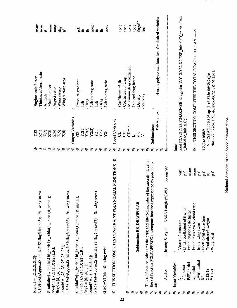
4. A/C Range Optimization Model.

Table A1 shows the equations used in each of the BBs

for the aircraft model. Polynomial functions are repre-

sented by 'Pf0' with independent variables in the pa-rentheses. Each polynomial function is of the form:

(A22) PF =mo + mi*s T + (1/2)*S*Aij*S T

Where S is the vector of independent variables, and Ao,

Ai, and Aij are coefficient terms.

In calculating the polynomial functions using eq. A22,terms in the S vectors are in the same order as they

appear in Pf0 in Table AI. The off diagonal terms of

Aij are random numbers between 0 and 1. For this

model, they are

O.4252A_j = 0.0329 0.8856

0.0878 0.7248

0.6357 0.7435 0.1138

- - 0.3657 0.0019

0.1978 0.0169

The remaining coefficient are:

• 0--->

• Fol --->

• _1 --->

Ao = [1.0]; A_ = [0.3 -0.3 -0.3 -0.2];

A_ = [0.4 -0.4 -0.4 0];

Ao = [1.0]; Ai = [6.25]; &i = [0];

Ao = [1.0]; Ai = [-0.75 0.5 -0.75 0.5

• o2 --->

• _3--->

• _4 --->

• _5 --->

• Fo2 --->

• Fo3 --->

• dp/dx --->

• Temp --->

0.5]; A_ = [-2.5 0 -2.5 0 0];

Ao = [1.0]; A_ = [-0.5 0.333 -0.5 0.333

0.333];Aii=[-1.111 0-1.111 00];

Ao = [I.01; A_ = [-0.375 0.25 -0.3750.25 0.25]; Ai, = [-0.625 0 -0.625 0 0];

Ao -- [! .0]; A_ = [-0.3 0.2 -0.3 0.2 0.2];

Au = [-0.4 0 -0.4 0 0];Ao = [1.01; A_ = [-0.25 0.1667 -0.25

0.1667 0.1667]; Au = [-0.2778 0

-0.2778 0 0];

Ao = [1.0]; Ai = [0.2 0.2]; Aii= [0 0];

Ao = [1.0]; Ai = [0]; aii= [0.04];

Ao = [1.0]; Ai = [0.2]; Aii= [0];

Ao = [1.0]; & = [0.3 -0.3 0.31;

Aii = [0.4 -0.4 0.4];

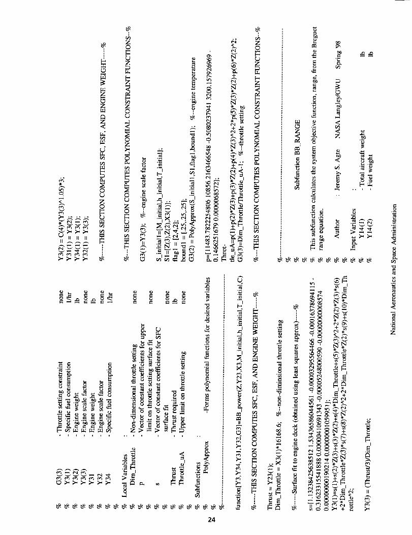
Equations for SFC and the upper constraint bound on

throttle setting in the Propulsion BB are polynomials

representing surfaces fit to engine deck data (AIAA/

UTC/Pratt & Whitney, 1995/96).

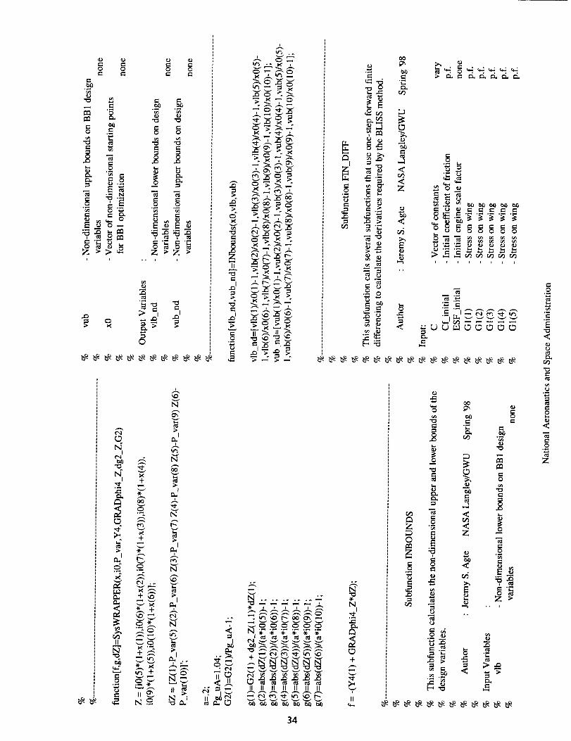
5. AJC Range MATLAB Code.

Included in the following pages is the MATLAB code

for the aircraft range optimization model. The con-

strained optimization routine used in BB 1OPT,

BB2OPT, BB3OPT, and SYSOPT may be found in

MATLAB's Optimization Toolbox and is based on a

Sequential Quadratic Programming method. The finite

differencing subfunctions in FIN_DIFF are simple one-

step forward finite difference codes that use a 1 percent

step increment.


15

OC

-----.o ._ ..,-

_'_ .o

_:_

__ "'=_

• _ <_ _._

_. >. }, 1>. >. ;> >

_ _._ . _

N N I N

_<_ _ _ _

>

_ _ _ _._._ ._,

• .o > > ._ ._ > _

_._ _:_;- _-_;-_;-

i , i a i i i

°_

Ze_

¢.i

Z

ili_ii iiiiii_ i i : : : • : i : i i• _ • i i i ! ! : ! : ! • i

: "© : :© :_ : : _ _ ::__ :_ :_ : :_

16

0

c_O0

p--. _0

><

[--,m

=-

c_ ._. ,..] -_ "_} c_I

°ii °_ °_ ° _ i

o _--

_g_._

_1_.t_t_-__.:_

_ .£ _--

0°_

°_

.<{l,}

c_

t-Lr_

"0

C}°_

.o<

0

c_

Z

17

.o

o_

-=

<

P_

<

.._

Z

+

N I

I

+ N IN I

_N+ I

I

Nf _,

•-_ +

_- 0l_ e..,lI r_

m

II II l_l

18

o

Ne.

-_,

Z

- E EII 0 0

cc cc

_ o__

i i l i i .° i i , l i

c_

E g

e-

e_

No _ _ _ _ u oNe_o

•- .om_ _

0

.= -_

_-_-

-_- ._ _

''-i

MI '= M

{

_ t.1

t'¢5

g.

I

I

t'N e_I I

t"l t'_

t",l I m I m I _

t'N I c'l I m I _

_._

e-

e_

_ _ _ _-

I._

;_... o ;>,..- o ,_i_i _'._

--, -_, _,_

-- _=_ _

I

r._

0

¢.j,

.._"_=

.r-

;_ e- e_ I::L e- e-...-

e_

z< :_ -_._ ._

._ ._

_ "_ _" = ._

°.

e_

e_

19

e-O

"r-

e_

e-

e-,

O

Z

r-

T+c_

..=I

¢_, ..-.+.

+...+

C_, IIII +..-..

+

v

<-

l N

V+ *

<.2

m_.

× N_--.

.1_ <' "2.

"_ {'4 _.._ _'-_

N M.-._

©

-+_ + o

N I II II II

____ ',

_d.__._ _ ___. ___ _ _

+•-_ _._._ _oo_'_ "N_

_ _-- o _'- _ .-'_.B

llntllllll ,.iiii I

z+

"¢3

"O

.o

O

O

°.

21

ZO

8

©

Z©

N©

Z©N

;t

_ ,:.a

._. -_ ..

,.._11 _ ,....1I

"_ m N

,-.-r ".-_ _r._ I

•= x+ ;a Z+ g

NI'-"N_2_T;_ _ ._-

I

; u.

N 0 ._

ell

N © "-" l

" .-= z _' Z

J "-"

;m'+ +..+-- *N*

=+'d : N+_.

++ -+

• c,I£ --._-_ r-. _ _

"+ =v. 2._r%

+_ -_

e. +..+

-_, "I I _ r_

,

e',O

e_

8

e=

o

Z

0°_

i i i i i i i

= 6 6

..iiiiiii

_}_ NNNNN

o !

IIIIII

I:

>

=

,2

Eo

B

.<

.=- I

U U

-_,

m _

_ Z

_._. U-I

t'N _

6 __.'= := g:_ 1,e .= J _-

°_ _

_0

*

• ¢%

_9

_momc, i

II oC,I.-,>_N

22

,.-aOeL_D

I

.o

"_o

_ ._.

",_

_ z_

o _

o.

do

e-

=

.__

_a

> _= ,- d.d._ d.

O

= .=O

'_ _

_-_ _.-_='_ _._ _

i i i i i i i i

.o

t,=

<

c_°_

i-=

.o<

e-,O

Z

'a

: .= :

Z _ Z

1

Z

z } zO . O

m

o :,-2." o

Z ,= i 2:o _ _ o

., t'q _ [,_

i

¢)

¢.j,

0

;.E..

r-.-

oo rj

* N- E

_ E g

od 6 * "__,_ t"-

P_ _ o

N II ,-" 0

II o ;;,.., m,II "

_ > "5""u _ i

t-,

,I ,,e,

._. o

_O

O "_.1

._ _

°_

t",l _

II

Z"Oo0

o

5-,

N

e_

+

II

.:-te-q

_q

IIA

OO

<r_

<Z

_o<

_6

_ ""

g88_8 8g _ 8_

_, _ 0 0

._._. '_ ,_ _ =

•= -= "= _ _oa ,..

i _ i i i i _ i i i i i .. _ i

•- ._ :E._ = _

U I_ I NNN NN NN _D_

N1::

N

O

e'_

N

O

_ N

N o

23

0

E<

o_

,o_J

<

r!o

Z

tt3

m

II II il

('_ r¢3 ('_ ("q

Z

_3

©r.)Z©

Ii

ZO

L)

Z0

2

e-

e-

?

O "

0 _ "=

0 .H % .H

o__°___ _'__ N_ 2"-.-- ""B

_ i..-_

0, _

o,, N. _.)

r_ +_. [-.,_ Z

t'N

,.. NI r,_

_- *_ z

(",1

oo

° _o," "-- ,..

--- ©'_" + ,-..

_.._ .s:,

oo 1"_ I

__o___

m

_a ,, _ _ " .."o

"o

m m

,._.$ ot..,)

._

_ _ o_ 0 __o _ _g_

i i i i i i i ., i i i i i ,.

oN

_ _ _,_m_m

24

.HI 1

o

DO

z

4

_4 _n

e.o [-'

D

o

•= .o

..=

O_

• "_

m

e.

< ._

g z ._

< _._

_= _

t) oo

°_._ i_ _

r¢3

r-,) o_

._ +g< ,-.,'_ ('NI

_= =

_ggeg ¢-gg _ d

N_e_ ea _v_ e

o

<

t..)

_3"O

ml

e=o,9.<

e-o

Z

{} II oo

-- 0 D

.--2II

a:: . II {}

o i,= ..

o {_ o _ o o o o o o

_=._

_ o: -- ___ _ " _ "

___ __ __i _ _ .. i i i i °. i i i i i

__

•_ ._ _0 -_..'_ _ _'--

..__

E _

o

o

_o

-,__ __'_ .o _

•_ _ _ __--'- _ _

i i i i _ i i .. i .. i

_NNNNNNN

©

.2., ..

z o

o _ _ o

0 _ _ 0

o. _ _

E _

25

e- J=

_ -_-_e-

_ -_

e_

e-,0

<

8

2<

o

z

e,,i

Z

0

00

Z ,--0

Z

_a _a

¢o

e _Z

m 0_ Z

M

o £

° E0

° _0,'_

@

_ _ "_ 0

< _._

'- _' 2

t" ' "

<

0C_

Z0o.<

0

00000

00000

_ddddd

°_ ._

°,

_ + ._._

°° .'_

I

I

t',l

+0_-,

o@_'_ I

+r..) o

e_

ii

0

c_

o

<

0

Z

26

o.O

E_-_ o

_E _

_ o_

>>_>i i i

0 =

_o

e-. e.,

,-_ e-.

na e_

0 0 e-.

•= 2 "_e-,

= ,-' t= :_7"_,.o o o¢J

g_g__

°° i i i t

e_0

w_i i

0 0

6

©

0°_

27

0

"E

"0<

(,_

"0

c_

c_

o<

0

mlZ

0a

o o o

_-_ ._

. _c N ._ . =

>>> e._a

Og)._

<=,{,<=> _'_ ._ "_

• _ _

N'-_

,---,[,.)

_'=

_ J

_-_

!-?_,_M

o_

e_

_ °_

_ •

_5

"N

e-

I

I::L I _1

._ +

__ __._ _

I

I

_ °_

__ .__ -

.... _,__,, ,,_

o_

O

m

..=

00

•= _

0 0

_ M

"=8

I= > m

e_

-_ ._. o=

r_ '_'_

_ .

>vi

;>>>• - i i i i

..

"_a=

_D

•_ _ _

"-_ _ !_ °

• _ _

o_ _ _._

28

O

.<

¢.a

e'_

"O

._

e-,

.<

O°_

Z

a} _ ¢}{-. _ c-o o o

¢} {2

m m _

•- 2 -_

0 0 0

"_ "_ o '-

• _ !_

.. i i i i

> __ -_ 0

00

°,_ . _

u E_g.g

i i

r_ 6e-

x('xl

I

¢-

,.1:_ I

-U

_u

O=

II -..r

e4 i

,- [-

.n" ._

°_

U

• • • _ H _ ._

oooooo o___ _ _ I"_ _ 0 0 0 0 0 0 _ _

©

n:

0

{.)

• 0 0 , 0

29

©

¢-0

<

e_

<

0

Z

_3

Ca

-g

e.a

i¢/J

f= .=

=So_

.= ..=

..= ..=LT._i [-l_I

uaeq

,..-,

>_ e4.,,.,

>

- _:aD

o_tO t _

eq;_ "-" 4

6 . i_ " ",..,:2.= ..= X _ :_

o_

,_'g

©

ge,,)i=

,.e

@

0

=g

°_

..g__

z _ B _ .__"

_._ oo i _ i ,

<

g,

m

_,=

¢,q

gU

=S

-=.

..=

@

e_

m d= "N _ "_= eO U "_

o.

-_ .=

•. ..., D _ >_ )" > N N N N N NeL

.=

{D

{g

._

=g'_ .=

>>> _8• o1_1 o.i

•_ ..=>d

©

30

e-@

<

ca

m_

8o_

==

.<

Z

i

xcq

_4

>I

s."-6

..{:I

E

o

C_II

o I

o

_..=_=."

X,-

=.__' o .__.= ,-

c,o {/} r_o ¢_ {1_ o'}

_oooooo•"; _'= ===.=.=o o o o o o

:,-2_" _ rd

•,.-, > [--,

•-= =.' "di

,.= 0" .=

-- ..= .=.- _ -_

>I x ["q"

5 _

c_ "_= _ _"L; _'1--',-=>.'

,.vUJck,C_

C_

=o

r.w0

..=

orj,

o

E =o o

e.. ow,.,

N

oO

.o_ >., >.

,-. > >

I-,

< ._

z _-_

_.'=>> N

_ t..,I "=.=-,< ,_L>_ .=

e'_

> e-, e-,

e., =

._ e" ¢"

.!i_ _ _ __'_

i i i i i i i i i i _ i

.E

c-o¢j

=

o "=

"- _

$.._ __._--

._

i i

e-

31

¢-o

"E

<

P0

<

e-o

z

o_

° _ _ _

©;}..,r./'}

t,,}

{}

0

¢}

.fl

[.-,

E

r,_

O0

,-]

.<<Z

.<

E

," ,-,.= =-81=

,,,-!

E _ _, _,"= _-u "_

o

_ ..o ..

n_::_ _>z _-z

o°_

.-_ _

N

.1::}

°_

°•: _-_ ._

• _ _ ._ _-_"_o ._ _

_'_ _ _

_._ _

iii .,_11 ..

_}'_ _ .....o_

_ _ _NNNNNN

© m

32

I

,..-r Io_

I

t'-I

II +

_ _u e4

,K

.o

.<

r!

.o<

o

z

N I

o_

i

II

G

o

ta0

o

o <

= <,2 Z

>

o o

-_ _._

=_ __

_ }- _-

__'_ _. _

o ._

.- -__._ _ -- ,,

_ _.__,-_ _._

.= _ _ _o_ _

o o

_ _=

i i i .. i i

N

c_ •_ _ <

N N N N N N u- _ _ _ _

©

_N._ "_

e_ _ii -_-'__ _-_

_;>> o

0 0

o

_) _ ._

.oU__:_ ,

°_

e-"

r_

33

Nil _

.=- --_ t"_

N

r_

_'N

_ ._'-"

D

I

_:m ¢-

I

" D

_" 2.'

a. q

.... e," N

- °° _,---'_',, _ _"Z'Z'_75 _ eN eeg N _

o

E

<

<

.o

Z

o

{.}

Z

},

.o

H

0 0

O _

_ NO

z Z-- i i

;> ..al ..ot

©

N

+

"'-'- N

°_ [_

_,+ --,-.

_;.- N

N_

__ _" ,._

_.a.,

°_

N__

w_ w

34

Z

_m

_ ,--1

_ <C_

_ z

e',O

I: I _'_ _'_ _'_ _-_

©

°_

N

H

_ _ o

"r. ,,-

O

"2

<

r_

8

e-,

R<

O

z

ID

, 1 , t i

NN_NN

0

<

o

8°_

c-

O

<

.o

Z

35

6=

,.2

.r./_ o_.

C,'¢ .c_

='

• '_ c_

-= ._ ;>., -=

•_ .= =

.=_ .= _ .= -_

-_ -_ .=_ .=. .=-

_ _ i /-" /'_ /'_

,_ ce_ eel

m

= ,,_ =l_,j , , , I

._ °_

._ ._

._ o_

,,_I I ,_.I I '_ ._ .._

tel _ c,_

,._._ ,,,-._ {,q (-.q

_-..i I C,.,.II

[_.,

Iii

<

1 II

_. <

°_

0.0

_ -':' _ ,'-' {') _ ff'.,1 {,.}

°O) "_ ° r.) •

NNNN _ _

_8__99Ngsgs

_--B _c_-.II :t _>'_1 I )_1 _'% Nt NI NI NI NI NI NI

36

O

<

{.}

<

Z

N I ,_I _'_ _ _-_

_ e_ _ _ _0

°_

¢-

•= 7= =

I

I

N _4

×, ×, ×,e_

J

?

i

I

. Ie-,

_ H

c_

.. .- N I b"] I

,-.r I

°_ _

°_j ._

0__ ._.

• _ J•- I e-

N _m M

M m

M m"

N "" N 1 M 1

II N II II

"r. I

¢-O

?ii

0_

°_

I I

O

¢-

O°_

Z

37

REPORT DOCUMENTATION PAGE l Form_pr¢_OMB NO. 0704-0188l

Public reporting burden for this collection of information is estimated to average 1 hour per response, including the time for revmwing i_ons, searching existing data sources,cotgathe,dng _ mainta.ining the data needed, and complating and reviewing the c_.lecbon of information. Send comments regarding this burden estimate or any other aspect of this

lect_0_ OTinformation, =ndudtng suggestions for reducing th=sburden, to Washington Headquarters Services, Directorate for Information Operations and Reports, 1215 JeffersonDa_s Highway, Suite 1204, Arlington, VA 22202-4302, and to the _ of Management and Budojst, Paperwork Reduction Project (07040188), Washington, DE; 20503.

1. AGENCY USE ONLY (Leave blank) 2. REPORT DATE

Aul_ust 19984. TITLE AND SUEfiTLE

Bi-Level Integrated System Synthesis (BLISS)

6. AUTHOR(S)

Jaroslaw Sobieszczanski-Sobieski, Jeremy S. Agte, and Robert R.

Sandusky, Jr.

7. PERFORMING ORGANIZATION NAME(S) AND ADDRESS(ES)

NASA Langley Research Center

Hampton, VA 23681-2199

9. SPONSORING/MONITORINGAGENCYNAME(S)ANDADDRESS(ES)

National Aeronautics and Space AdministrationWashington, DC 20546-0001

3. REPORT TYPE AND DATES COVERED

Technical Memorandum5. FUNDING NUMBERS

509-10-31-03

8. PERFORMING ORGANIZATIONREPORT NUMBER

L-17778

10. SPONSORING/MON_ORINGAGENCY REPORT NUMBER

NASA/TM-1998-208715

11. SUPPLEMENTARY NOo-S

Sobieski: Manager, Computational AeroSciences, and Multidisciplinary Research Coordinator, NASA Langley

Research Center; Agte: Graduate Research Scholar Assistant, The George Washington University, LT, U.S. Air

Force_ Sandusky: Professor t The George Washington University.12a. DISTRIBUTION/AVAILABILITY STATEMENT 12b. DISTRIBUTION CODE

Unclassified-Unlimited

Subject Category 05 Distribution: Standard

Availability: NASA CASI (301) 621-0390

13. AB_/HACT (Maximum 200 words)

BLISS is a method for optimization of engineering systems by decomposition. It separates the system level

optimization, having a relatively small number of design variables, from the potentially numerous subsystem

optimizations that may each have a large number of local design variables. The subsystem optimizations are

autonomous and may be conducted concurrently. Subsystem and system optimizations alternate, linked by

sensitivity data, producing a design improvement in each iteration. Starting from a best guess initial design, the

method improves that design in iterative cycles, each cycle comprised of two steps. In step one, the system level

variables are frozen and the improvement is achieved by separate, concurrent, and autonomous optimizations inthe local variable subdomains. In step two, further improvement is sought in the space of the system level

variables. Optimum sensitivity data link the second step to the first. The method prototype was implemented

using MATLAB and iSIGHT programming software and tested on a simplified, conceptual level supersonic

business jet design, and a detailed design of an electronic device. Satisfactory convergence and favorable

agreement with the benchmark results were observed. Modularity of the method is intended to fit the human

organization and map well on the computing technology of concurrent processing.

14. SUBJECT TERMS

Parallel Processing; Optimization by Decomposition; Engineering System Design

17. SECURITY CLASSIRCATICNOF REPORT

Unclassified

18. SECUHiTlf CI.ASSIRCATICNOF THIS PAGE

Unclassified

NSN 7540-01-280-5500

19. SECURITY CLASSIFICATIONOF ABSTRACT

Unclassified

15. NUMBER OF PAGES

4216. PRICE CODE

A0320. LIMITATION

OF ABSTRACT

Standard Form 298 (Rev. 2-89)Prescnbed by ANSI Std. z-a9-18298-1(_

38

Bi-Level Integrated System Synthesis (BLISS) - NASA · BI-LEVEL INTEGRATED SYSTEM SYNTHESIS (BLISS)...

Documents

Transcript of Bi-Level Integrated System Synthesis (BLISS) - NASA · BI-LEVEL INTEGRATED SYSTEM SYNTHESIS (BLISS)...