Beyond fractals: surrogate time series and fields

Victor Venema and Clemens Simmer

Meteorologisches Institut, Universität Bonn, Germany

Cloud measurements: Cloud measurements: Susanne Crewell, Ulrich Löhnert Susanne Crewell, Ulrich Löhnert , Sebastian Schmidt, Sebastian Schmidt

Climate data & analysis:Climate data & analysis:Susanne Bachner, Alice Kapala, Henning RustSusanne Bachner, Alice Kapala, Henning Rust

Radiative transfer & analysis: Radiative transfer & analysis: Sebastián Gimeno García , Anke Kniffka, Sebastián Gimeno García , Anke Kniffka,

Steffen Meyer, Sebastian SchmidtSteffen Meyer, Sebastian Schmidt3D cloud modelling:3D cloud modelling:

Andreas Chlond, Frederick Chosson, Andreas Chlond, Frederick Chosson, Siegfried Raasch, Michael SchroeterSiegfried Raasch, Michael Schroeter

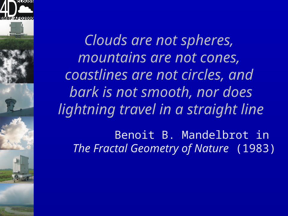
Clouds are not spheres, mountains are not cones,

coastlines are not circles, and bark is not smooth, nor does

lightning travel in a straight line

Benoit B. Mandelbrot in The Fractal Geometry of Nature (1983)

Fractals

Implied: nature is fractal Fractal, self-similar

– Zoom in, looks the same– Structure measure is a power law of scale– Linear on a double logarithmic plot

Beginning of complex system sciences? Structure on all scales

My experience: good approximation for turbulence and stratiform clouds, but often see different signals

The great tragedy of science — the slaying of a beautiful theory by

an ugly fact

Thomas Henry Huxley (1825–1895)

Content

Motivation – What I do– Radiative transfer through clouds– Basic algorithm

Case study – 3D clouds Validation - 3D clouds Structure functions of surrogates

Motivation – compare multifractals Conclusions More information

Motivation – Cloud structure

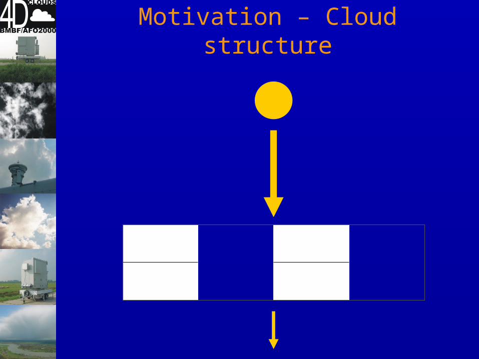
Motivation – Cloud structure

Motivation – Cloud structure

Motivation – Cloud structure

Motivation Can not measure a full 3D cloud field Need 3D field for radiative transfer calculations Can measure many (statistical) cloud properties Generate cloud field based on statistics

measurements

Nonlinear processes– Precise distribution

Non-local processes– E.g. power spectrum (autocorrelation function)

In geophysics you generally do not have full fields, but can estimate these two statistics

Time series

The iterative IAAFT algorithmSchreiber and Schmitz

DistributionFlow diagram Time series

Case study

Two flights: Stratocumulus, Cumulus Airplane measurements

– Liquid water content– Drop sizes

Triangle horizontal leg (horizontal structure) A few ramps, for vertical profile

Three cloud generators Irradiance modelling and measurement

Surrogates from airplane data

Three reconstructions

Irradiances stratocumulus

Irradiances cumulus

0.0 0.2 0.40.0

0.1

0.2

0.3

0.4

0.5 aircraft measurement

CLABAUTAIR MC IPA

PD

F(F

)

F [W m-2 nm-1]0.0 0.2 0.4

0.0

0.1

0.2

0.3

0.4

0.5SITCOM

MC IPA

F [W m-2 nm-1]0.0 0.2 0.4

0.0

0.1

0.2

0.3

0.4

0.5 MODIS cloud cover & Reff

MO

DIS

clo

ud c

over

(60

%)

IAAFT MC IPA

F [W m-2 nm-1]

0.0 0.5 1.00.0

0.1

0.2CLABAUTAIR

MC IPA

ground measurement

PD

F(F

)

F [W m-2 nm-1]0.0 0.5 1.0

0.0

0.1

0.2SITCOM

MC IPA

F [W m-2 nm-1]0.0 0.5 1.0

0.0

0.1

0.2M

OD

IS c

loud

cov

er &

Re

ffIAAFT

MC IPA

F [W m-2 nm-1]

MO

DIS

clo

ud c

over

(60

%)

0.0 0.2 0.40.0

0.1

0.2

0.3

0.4

0.5 aircraft measurement

CLABAUTAIR MC IPA

PD

F(F

)

F [W m-2 nm-1]0.0 0.2 0.4

0.0

0.1

0.2

0.3

0.4

0.5SITCOM

MC IPA

F [W m-2 nm-1]0.0 0.2 0.4

0.0

0.1

0.2

0.3

0.4

0.5 MODIS cloud cover & Reff

MO

DIS

clo

ud c

over

(60

%)

IAAFT MC IPA

F [W m-2 nm-1]

0.0 0.5 1.00.0

0.1

0.2CLABAUTAIR

MC IPA

ground measurement

PD

F(F

)

F [W m-2 nm-1]0.0 0.5 1.0

0.0

0.1

0.2SITCOM

MC IPA

F [W m-2 nm-1]0.0 0.5 1.0

0.0

0.1

0.2M

OD

IS c

loud

cov

er &

Re

ffIAAFT

MC IPA

F [W m-2 nm-1]

MO

DIS

clo

ud c

over

(60

%)

Validation – 3D clouds

3D models clouds -> 3D surrogates Full information, perfect statistics Test if the statistics are good enough

The root-mean-square (RMS) differences are less than 1 percent (not significant)

Significant differences– Fourier surrogates: distribution is important– PDF surrogates: correlations are important

Trivial problem, but just numerical result

“Validation” time series

1D climate time series and clouds 4th order structure function

– Surrogates more accurate (as multifractal)

Full information, perfect statistics Numerical test how good the statistics are

400 600 800 1000 1200 1400 1600 18000

5

10

Time (pixel)

Va

lue p-model

1894 1894.5 1895 1895.5 1896 1896.5 1897 1897.50

20

Time (year)

Ra

in (

mm

/d)

daily rain sums

1828 1828.5 1829 1829.5 1830 1830.5 1831 1831.5

500100015002000

Time (year)

Ru

no

ff (m

3/s

)

runoff Burghausen

1818 1818.5 1819 1819.5 1820 1820.5 1821 1821.5

2000400060008000

Time (year)

Ru

no

ff (m

3/s

)

runoff Cologne

0 200 400 600 800 1000 1200 1400 16000

0.2

0.4

Time (s)

LW

C (

g m

-3)

cumulus

0 200 400 600 800 1000

0.4

0.6

Time (s)

LW

C (

g m

-3)

stratocumulus

1894 1894.5 1895 1895.5 1896 1896.5 1897 1897.5-10

01020

Time (year)

Te

mp

. (°C

)

temperature

Structure functions

Increment time series: (x,l)=(t+l)- (t)

SF(l,q) = (1/N) Σ ||q

SF(l,2) is equivalent to auto-correlation function

Correlated time series SF increases with l Higher q focuses on larger jumps

4th order SF cumulus

100

101

102

10-4

10-3

time (s)

Fo

urt

h o

rde

r st

ruct

ure

fun

ctio

n

MeasurementSIAAFT surrogateIAAFT surrogateAAFT surrogateFARIMA surrogateFARIMA + IAAFT surrogate

Error 4th order structure function

SIAAFT IAAFT AAFT Fourier PDF FARIMA FARIMA + IAAFT Multifractal

Bias

P-model 0.018 0.019 0.016 0.071 0.065 0.068 0.020 0.017

Rain Potsdam 0.0027 0.0021 0.0038 0.093 0.0023 0.099 0.0029 0.0020

Runoff Burghausen 0.011 0.0069 0.029 0.076 0.081 0.076 0.023 0.028

Runoff Cologne 0.016 0.016 0.025 0.064 1.6 0.043 0.034 0.19

Cumulus 0.012 0.0080 0.016 0.076 0.044 0.063 0.0070 0.029

Stratocumulus 0.018 0.017 0.018 0.026 0.49 0.042 0.038 0.028

Temperature 0.0027 0.0037 0.016 0.0062 1.7 0.0060 0.0055 0.073

Variabilty

P-model 0.18 0.19 0.17 0.71 0.65 0.68 0.20 0.17

Rain Potsdam 0.032 0.028 0.048 0.92 0.036 0.99 0.037 0.020

Runoff Burghausen 0.12 0.081 0.31 0.76 0.81 0.76 0.24 0.28

Runoff Cologne 0.16 0.16 0.26 0.64 16 0.45 0.35 1.9

Cumulus 0.14 0.10 0.20 0.76 0.45 1.5 0.13 0.29

Stratocumulus 0.19 0.18 0.19 0.26 4.9 0.46 0.40 0.28

Temperature 0.034 0.040 0.17 0.066 17 0.062 0.057 0.73

Generators

Iterative amplitude adjusted Fourier transform algorithm – Schreiber and Schmitz (1996, 2000)– Masters and Gurley (2003)– ...

Search algorithm– Simulated annealing (Schreiber, 1998) – Genetic algorithm (Venema, 2003)

Geostatistics: stochastic simulation– Search algorithms– Gaussian distribution

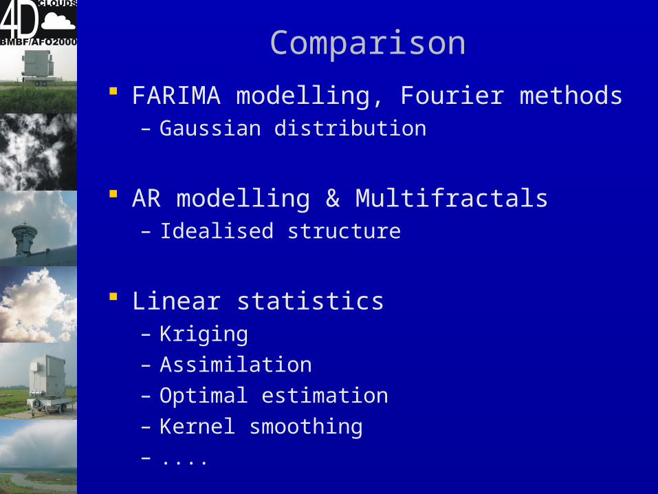
Comparison

FARIMA modelling, Fourier methods– Gaussian distribution

AR modelling & Multifractals– Idealised structure

Linear statistics– Kriging– Assimilation– Optimal estimation– Kernel smoothing– ....

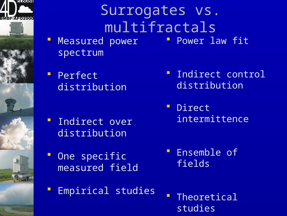
Surrogates vs. multifractals Measured power

spectrum

Perfect distribution

Indirect over distribution

One specific measured field

Empirical studies

Power law fit

Indirect control distribution

Direct intermittence

Ensemble of fields

Theoretical studies

Cloud structure is not fractal Scale breaks Waves Land sea mask …

Satellite pictures: Eumetsat

Land surface is not fractal

15 Reasons the surface is not uni-fractal (Steward and McClean, 1985):– Fractal landscape have the same number of

tops and pits– Glacial cirques has a narrow size range and

size dependent shape

Conclusions

IAAFT algorithm can generate structures– Accurately– Flexibly– Efficiently

Many useful extensions are possible– Local values– Increment distributions– Downscaling

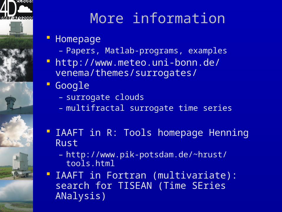
More information Homepage

– Papers, Matlab-programs, examples http://www.meteo.uni-bonn.de/

venema/themes/surrogates/ Google

– surrogate clouds– multifractal surrogate time series

IAAFT in R: Tools homepage Henning Rust– http://www.pik-potsdam.de/~hrust/tools.html

IAAFT in Fortran (multivariate): search for TISEAN (Time SEries ANalysis)