Best Practices for Measuring Discharge with Acoustic ... · 1 Best Practices for Measuring...

1

Best Practices for Measuring Discharge with Acoustic Doppler Current Profilers

By David S. Mueller1, Chad R. Wagner2, and Michael F. Winkler3

Report formatted consistent with USGS guidelines. Report to be reformatted and published by the U.S. Army Corps of Engineers.

1Hydrologist, U.S. Geological Survey, Office of Surface Water, 9818 Bluegrass Parkway,

Louisville, KY 40299

2Hydrologist, U.S. Geological Survey, North Carolina Water Science Center, 3916 Sunset Ridge

Road, Raleigh, NC 27607

3Research Hydraulic Engineer, CEERD-HN-N, 3909 Halls Ferry Road, Vicksburg, MS 39180

3

TABLE OF CONTENTS

ABSTRACT ..................................................................................................................... 10 INTRODUCTION........................................................................................................... 10

Purpose and Scope .................................................................................................................... 10 Applications .............................................................................................................................. 11 Discussion of Instruments ......................................................................................................... 12

PREDEPLOYMENT PREPARATION ........................................................................ 14

Data Management ..................................................................................................................... 14 Naming Convention .............................................................................................................. 14 Data Storage and Archival .................................................................................................... 14

Instrument and Site Considerations .......................................................................................... 15 Limitations of Acoustic Profilers .......................................................................................... 15

Effect of Sediment ............................................................................................................ 15 Unmeasured Areas in a Profile ......................................................................................... 16

Configuration and Characteristics ......................................................................................... 17 Compass Considerations ....................................................................................................... 20

Instrument Quality Assurance ................................................................................................... 20 Software and Firmware Procedures ...................................................................................... 20 Instrument Tests .................................................................................................................... 21

Beam Alignment Test ....................................................................................................... 21 Periodic Instrument Check ................................................................................................ 21

Ancillary Equipment ................................................................................................................. 22 GPS Requirements and Specifications .................................................................................. 22 Echo Sounder ........................................................................................................................ 23 Instrument Deployments and Mounts ................................................................................... 23

Manned Boats ................................................................................................................... 23 Tethered Boats .................................................................................................................. 26 Remote-Control Boats ...................................................................................................... 28

Other Equipment ................................................................................................................... 29 Final Equipment Preparation and Inspection ............................................................................ 31

FIELD PROCEDURES .................................................................................................. 33

Site Selection ............................................................................................................................ 33 Pre-Measurement Field Procedures .......................................................................................... 34

Set Internal Clock ................................................................................................................. 34 Instrument Diagnostic Checks .............................................................................................. 35 Speed of Sound ..................................................................................................................... 35

Water Temperature ........................................................................................................... 35 Salinity .............................................................................................................................. 36

Compass Calibration ............................................................................................................. 36 Instrument Configuration ...................................................................................................... 37 Moving-Bed Tests ................................................................................................................. 39

4

Stationary Test, No GPS ................................................................................................... 40 Stationary Test, With GPS ................................................................................................ 41 Loop Test .......................................................................................................................... 42

Discharge-Measurement Procedures ........................................................................................ 44 Steady Flow Conditions ........................................................................................................ 44 Unsteady Flow Conditions .................................................................................................... 45 Critical Data-Quality Problems............................................................................................. 45 Boat Operation ...................................................................................................................... 46 Estimating Edge Discharge ................................................................................................... 47 Field Notes ............................................................................................................................ 48 Step by Step Procedure ......................................................................................................... 48

Post-Measurement Field Procedures......................................................................................... 48 OFFICE PROCEDURES ............................................................................................... 50

Preventative Maintenance ......................................................................................................... 50 Data Storage .............................................................................................................................. 50 Measurement Review Procedures ............................................................................................. 50 Data Quality Indicators ............................................................................................................. 52 Commonly Observed Measurement Problems ......................................................................... 58

REFERENCES ................................................................................................................ 60 APPENDIX A – BASIC ADCP OPERATIONAL CONCEPTS ................................ 63

General ...................................................................................................................................... 63 Measuring Velocity ................................................................................................................... 64

Narrowband........................................................................................................................... 64 Broadband ............................................................................................................................. 65

Computing Velocity in Orthogonal Coordinates ...................................................................... 67 Measuring a Velocity Profile .................................................................................................... 69 Computing Discharge ............................................................................................................... 69

Measured Discharge .............................................................................................................. 70 Top Discharge ....................................................................................................................... 71 Bottom Discharge ................................................................................................................. 73 Edge Discharge ..................................................................................................................... 73

APPENDIX B – COLLECTING DATA IN MOVING-BED CONDITIONS ........... 76

Cause and Effect of a Moving Bed ........................................................................................... 76 Methods to Identify a Moving Bed ........................................................................................... 78 Methods to Account for Moving-Bed Effects .......................................................................... 80 Using GPS with ADCPs ........................................................................................................... 80 Alternatives to Using GPS ........................................................................................................ 84

Subsection Method................................................................................................................ 84 Field Procedures: .............................................................................................................. 84 Processing Procedures: ..................................................................................................... 84

Section by Section Method ................................................................................................... 86 Azimuth Method ................................................................................................................... 87

5

Field Procedures: .............................................................................................................. 88 Processing Procedures: ..................................................................................................... 88

Loop Method ......................................................................................................................... 89 Field Procedures: .............................................................................................................. 90 Processing Procedures for Use as a Moving-Bed Test: .................................................... 91 Processing Procedures for Correcting Biased Discharge: ................................................ 92

APPENDIX C – DESCRIPTION OF WATER MODES ............................................ 94

SonTek/YSI RiverSurveyor Water Modes ............................................................................... 94 TRDI Rio Grande Water Modes ............................................................................................... 94

Mode 1 .................................................................................................................................. 95 Modes 5/11............................................................................................................................ 95 Mode 12 ................................................................................................................................ 96

APPENDIX D – BEAM ALIGNMENT TEST ............................................................. 97

Introduction ............................................................................................................................... 97 Description of Procedure .......................................................................................................... 97 Step by Step Procedure ............................................................................................................. 98

APPENDIX E – FORMS .............................................................................................. 100 APPENDIX F – MEASUREMENT REVIEW PROCEDURES .............................. 103

Teledyne RD Instruments ADCP ........................................................................................ 103 Sontek/YSI ADP .................................................................................................................... 107

7

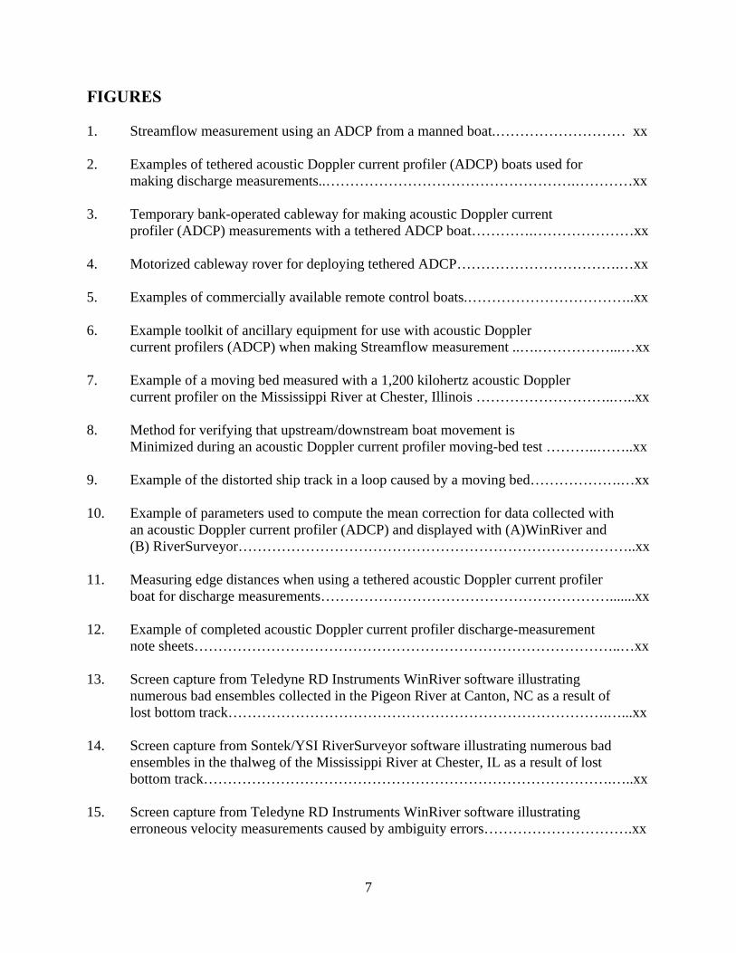
FIGURES 1. Streamflow measurement using an ADCP from a manned boat.……………………… xx 2. Examples of tethered acoustic Doppler current profiler (ADCP) boats used for

making discharge measurements..…………………………………………….…………xx 3. Temporary bank-operated cableway for making acoustic Doppler current

profiler (ADCP) measurements with a tethered ADCP boat………….…………………xx 4. Motorized cableway rover for deploying tethered ADCP…………………………….…xx

5. Examples of commercially available remote control boats.……………………………..xx

6. Example toolkit of ancillary equipment for use with acoustic Doppler

current profilers (ADCP) when making Streamflow measurement ..….……………...…xx

7. Example of a moving bed measured with a 1,200 kilohertz acoustic Doppler current profiler on the Mississippi River at Chester, Illinois ………………………..…..xx

8. Method for verifying that upstream/downstream boat movement is

Minimized during an acoustic Doppler current profiler moving-bed test ………..……..xx

9. Example of the distorted ship track in a loop caused by a moving bed……………….…xx 10. Example of parameters used to compute the mean correction for data collected with

an acoustic Doppler current profiler (ADCP) and displayed with (A)WinRiver and (B) RiverSurveyor………………………………………………………………………..xx

11. Measuring edge distances when using a tethered acoustic Doppler current profiler boat for discharge measurements…………………………………………………….......xx

12. Example of completed acoustic Doppler current profiler discharge-measurement note sheets……………………………………………………………………………..…xx

13. Screen capture from Teledyne RD Instruments WinRiver software illustrating numerous bad ensembles collected in the Pigeon River at Canton, NC as a result of lost bottom track…………………………………………………………………….…...xx

14. Screen capture from Sontek/YSI RiverSurveyor software illustrating numerous bad ensembles in the thalweg of the Mississippi River at Chester, IL as a result of lost bottom track………………………………………………………………………….…..xx

15. Screen capture from Teledyne RD Instruments WinRiver software illustrating erroneous velocity measurements caused by ambiguity errors………………………….xx

8

16. Screen capture from Sontek/YSI RiverSurveyor software illustrating an example of good and bad beam intensity data relative to detection of the streambed……………….xx

17. Screen capture from Teledyne RD Instruments WinRiver software illustrating an anomaly in beam intensities caused by interference in beam 1 from a side wall………..xx

18. Screen capture from Teledyne RD Instruments WinRiver software illustrating

highly variable boat speeds resulting from shifting the motor in and out of gear during the transect………………………………………………………………………..xx

19. Screen capture from Sontek/YSI RiverSurveyor software illustrating variation in

boat speed during a transect……………………………………………………………...xx

20. Screen capture from Teledyne RD Instruments WinRiver software illustrating spikes in the streambed profile………………………………………………………………….xx

21. Screen capture from Sontek/YSI RiverSurveyor software illustrating the effects of poor GPS data on the measurement of boat movement………………………………xx

TABLES 1. Characteristics of SonTek/YSI RiverSurveyor ADCPs…………………….………….xx 2. Characteristics of TRDI Rio Grande water profiling modes for 1,200 kHz and

600 kHz, in parentheses ADCPs ………………………….……………………...........xx

3. Advantages and disadvantages of acoustic Doppler current profiler (ADCP) mounting locations on manned boats…………………………………………………...xx

4. List of ancillary equipment to be included in acoustic Doppler current profiler (ADCP) toolkit for use with ADCPs when making streamflow measurements………...xx

9

CONVERSION FACTORS AND VERTICAL DATUM CONVERSION FACTORS Multiply By To obtain meter(m) 3.281 foot(ft) meter per second(m/s) 3.281 foot per second (ft/s) cubic meter per second(m3/s) 35.315 cubic feet per second (ft3/s) kilometer(km) 0.621 mile (mi

foot (ft) 0.0328 centimeter (cm) VERTICAL DATUM Elevation, as used in this report, refers to the distance above or below sea level.

10

BEST PRACTICES FOR MEASURING DISCHARGE WITH ACOUSTIC DOPPLER CURRENT PROFILERS

ABSTRACT The use of acoustic Doppler current profilers (ADCPs) from a moving boat is now a

commonly used method for measuring streamflow. The technology and method for making ADCP-based discharge measurements is different from the traditional discharge measurements made with mechanical meters. Although the ADCP is a valuable tool for measuring streamflow, it is only accurate when used with appropriate techniques. This report presents guidance on the use of ADCPs for measuring streamflow, based on the experience and published reports, papers, and memoradums of the U.S. Geological Survey. The guidance is presented in a logical progression from predeployment planning to field-data collection and finally to postprocessing of the collected data. Acoustic Doppler technology and the instruments currently (2007) available are also discussed to highlight the advantages and limitations of the technology. More in-depth, technical explanations of how an ADCP measures streamflow and what to do when measuring in moving bed conditions are presented in the Appendices. It is important that the ADCP user not only know the proper procedures but that the user also understand why those procedures are required, so that when the user encounters unusual field conditions the procedures can be adapted without sacrificing the accuracy of the measure data.

INTRODUCTION The acoustic Doppler current profiler (ADCP) has evolved during the last 25 years from

being an experimental instrument capable of measuring velocity and computing discharge in deep water (greater than 3.4 m) to an instrument that is commonly used to measure water velocity and discharge in streams as shallow as 0.3 m deep (Christensen and Herrick, 1982; Simpson and Oltmann, 1993; Oberg and Mueller, 2007). The development of the ADCP provides the hydrographer and engineer with a tool that can greatly reduce the time for making discharge measurements and can permit measurement of water velocities at a spatial and temporal scale that was previously unattainable. These instruments are used regularly to measure riverine and estuarine water discharge, to collect data for hydrodynamic model calibration and verification, to assess aquatic habitat, and to study sediment transport processes. Although the use of the ADCP has become common, proper instrument configuration, data collection and post-processing procedures are required to collect accurate and reliable data.

Purpose and Scope The purpose of this report is to present the procedures (and supporting information) that

should be followed when using an ADCP from a moving boat to make water discharge measurements. The procedures for predeployment preparation, field data collection, and processing of collected data are discussed. A detailed description of how an ADCP measures velocity and computes discharge and additional details on selected topics are presented in appendices.

11

Applications The measurement of unsteady, bidirectional, and other flows with non-logarithmic

velocity distributions has been a problem faced by hydrologists for many years. Dynamic discharge conditions impose an unreasonably short time constraint on conventional current-meter discharge-measurement methods, which typically last at least 1 hour. Tidally affected discharge can change more than 100 percent during a 10-minute period. In addition, bidirectional flows caused by density currents are common in tidally affected areas and have been increasingly observed in freshwater environments where there is significant temperature gradient to cause a density current (Garcia, Oberg, and Garcia, 2007). Nearly all discharge measurements made using point velocity meters have assumed a standard logarithmic distribution of the horizontal velocity in the water column, however, wind-driven currents and very rough bottoms in shallow water may produce nonstandard profiles. The introduction of the ADCP into the coastal and riverine environments enabled the development of a discharge-measurement system capable of more efficiently and more accurately measuring flow in unsteady, bidirectional, and nonstandard conditions. In most cases, an ADCP discharge-measurement system is faster than conventional discharge-measurement systems and has comparable or better accuracy because ADCPs measure a much larger portion of the water column than conventional discharge-measurement systems. More efficient discharge measurements improve safety by reducing the amount of time a hydrographer is on a bridge, on a boat, or in the water. The reduction in measurement time realized by utilizing an ADCP is especially beneficial when trying to develop an index velocity rating (Ruhl and Simpson, 2005; Morlock and others, 2002) at sites with rapidly changing flow conditions. An ADCP can define the rating in the transitional range of flow that was otherwise indefinable with conventional discharge methods. In addition to measuring streamflow, ADCPs are used in a variety of other applications including:

• measurement of velocity fields for calibration of numerical models, hydraulic studies (i.e. safety zones near dams), habitat assessments;

• in-situ deployments for current measurements and aiding navigation;

• hydrographic surveys to measure channel bathymetry for use in hydrodynamic and habitat modeling applications; and,

• estimation of sediment concentration from acoustic backscatter (ABS).

The application of acoustic technology in rivers and lakes has provided data that prior to the mid 1990s would have been unavailable or extremely expensive and impractical to collect.

12

Discussion of Instruments The ADCP uses sound to measure water velocity. The sound transmitted by the ADCP is

in the ultrasonic range (well above the range of the human ear). The lowest frequency used by commercial ADCPs is around 30 kHz, and the common range for riverine measurements is between 300–3,000 kHz. The ADCP measures water velocity using a principle of physics discovered by Christian Johann Doppler (1842). Doppler’s principle relates the change in frequency of a source to the relative velocities of the source and the observer. An ADCP applies the Doppler principle by reflecting an acoustic signal off small particles of sediment and other material (collectively referred to as scatterers) that are present in water. The velocity measured by the Doppler principle is parallel to the direction of the transducer emitting the signal and receiving the backscattered acoustic energy. Typical boat-mounted ADCPs have three or four beams pointing between 20 and 30 degrees from the vertical. Three beams are required to obtain a three-dimensional velocity measurement. If a fourth beam is present an additional error velocity can be measured (see Appendix A for details).

In a boat-mounted system, the transducers are deployed beneath the water surface and aimed downward (Figure 1). Measurement of water velocity from a moving boat will yield the velocity of the water relative to the boat. ADCPs used in this manner account for the velocity of the boat by bottom-tracking or through the use of a Global Positioning System (GPS). Bottom-tracking determines the velocity of the boat by measuring the Doppler shift of acoustic signals reflected from the streambed. Therefore, the water velocity relative to a fixed reference is computed by correcting the measured water velocity with the measured boat velocity.

Currently (2007) ADCPs can be classified into two groups based on the techniques used to configure and process the acoustic signal, narrowband and broadband. Narrowband is typically used in the hydroacoustic industry to describe a pulse-to-pulse incoherent ADCP, however, the narrowband ADCPs can also operate in a pulse-to-pulse coherent mode for short ranges. This means that in a narrowband ADCP, only one simple pulse is transmitted into the water, per beam per measurement (ping), and the resolution of Doppler shift takes place during the duration of the received pulse. This characteristic results in a system that is simple to configure and operate, but the velocity measurements made using the narrowband technology are noisy (have a relatively large random error). Narrowband systems compensate for the large random error by pinging fast (up to 20 Hz) and averaging many pings together before reporting a velocity. Typical response from a narrowband system is a velocity profile measurement

Figure 1. Streamflow measurement using an ADCP from a manned boat.

13

every 5 seconds.

Broadband systems utilize a ping consisting of two or more synchronized acoustic pulses that are encoded with a pseudo random code. The encoded pulse allows multiple velocity measurements to be made with a single ping, thus reducing the random noise associated in the measured velocity. Broadband systems are more difficult to configure due to the effect of the lag between the two pulses and the processing of the complex pulse is slower than a narrowband system; however, the complex pulse results in a much lower random error and the pulse pair allows configuration of the instrument to minimize random error for a particular measurement conditions.

14

PREDEPLOYMENT PREPARATION Prior to collecting data with an ADCP it is important to establish standard procedures to

ensure that the data collected will be stored in an efficient and consistent manner, the ADCP is in proper working order, and the ADCP is the proper equipment for making the measurement. Proper preparation will help avoid delays in the field, ensure complete and accurate data collection, and produce data that are documented and retrievable for future use. The required predeployment procedures include:

1. establishing a policy for handling and storing the data;

2. ensuring that ADCP hardware and software are working properly and are configured consistent with the policies established by the user’s agency;

3. identifying other equipment such as GPS and boats that may be needed;

4. ensuring that the ADCP is capable of measuring the desired data for the expected field conditions; and

5. gathering and checking the ADCP and all ancillary equipment for use with the ADCP.

Data Management The ADCP and associated software can produce a large number of files. It is important that these files are stored in a manner that allows user’s to easily identify the location, date, and type of data stored in the files. Because of the volatility of digital data, appropriate backup and archival procedures should also be implemented.

Naming Convention Each agency or office should establish and document a consistent naming convention for data files. Names of files should always be unique and should be descriptive of the data contained. Site number, site name, measurement number, project name, project number, and date are some of the descriptive terms that could be used in a filename. Typically ADCP data collection software will add a suffix to the user-defined name to identify the type of data file (configuration, raw data, ASCII data, etc.) and to ensure the each file has a unique name.

Data Storage and Archival Each office or agency collecting electronic discharge measurement data should have a written policy on permanent file storage and archiving procedures. Procedures outlined are based on the assumption that an agency or office has existing systems and procedures for performing routine backups and permanent archival for electronic information stored on servers. This policy should detail file and directory naming conventions, server directory structure, how soon data must be placed on the server after it is collected, and how, when, and where server data will be archived on stable archival media (U.S. Geological Survey, 2005). Paper measurement notes associated with an electronic discharge measurement should be filed and archived with other paper discharge measurement notes in accordance with current office or agency policies and procedures.

15

Each discharge measurement with electronic data files should have its own directory that contains all of the files collected or created as part of the measurement. These files include but are not limited to raw data, configuration information, moving-bed tests, instrument checks, calibration information, and discharge measurement notes. The naming convention for the directories in the archival directory structure should include some combination of measurement number, measurement dates, water years, location, and/or instrument types.

Instrument and Site Considerations Any site-specific information, such as maximum water depths and velocities from

previous measurements, can be used as a guide for configuring the instrument for the measurement site. Notes about measuring conditions and locations from previous ADCP discharge measurements should be reviewed prior to the field trip.

Limitations of Acoustic Profilers The physics associated with sound generation from a transducer and then propagation,

absorption, attenuation, and backscatter in the water column result in specific limitations and characteristics of ADCPs. Limitations that are discussed in this report include the effect of sediment on backscattered acoustic energy and bottom tracking, and unmeasured areas of a profile associated with transducer draft and ringing and side-lobe interference. Additional limitations are imposed on ADCP measurements by the techniques used to configure and process the acoustic signal, which vary based on specific user configuration of the instrument.

Effect of Sediment The quantity and characteristics of the particulate matter (sediment, aquatic life, etc.) in

the water column can significantly impact the ability of the ADCP to make an accurate velocity measurement. Pure water is acoustically transparent because it has no suspended particulate matter to reflect the acoustic energy. The water must contain enough particulate matter for sufficient acoustic energy to be returned to the instrument for a velocity measurement to be made. Therefore, in clear streams it is possible to have insufficient material in the water column to allow an ADCP to measure water velocity. High sediment loads, which are often present during high-flow conditions, can have the opposite effect. High sediment concentrations near the streambed can cause the ADCP to have trouble discriminating the streambed from the suspended sediment concentration near the streambed and inaccurate water depth measurements result. It is also possible for the water to contain so much sediment in the water column that the acoustic signal is attenuated before it can travel through the water column and back to the transducer, preventing the ADCP from making a measurement. The sediment concentrations that trigger these limitations on ADCP operation have been observed but have not been quantified and will depend on the sediment characteristics and on the water depth. In general, low frequency acoustic instruments transmit more energy into the water and thus are more capable of penetrating high sediment concentrations than high frequency instruments.

During high flows, sediment transport near and along the streambed can cause a bias in the boat velocity determined from bottom tracking. Bottom tracking is used to determine the boat velocity and assumes that the streambed is stationary. Sediment transport near and along the streambed can cause a Doppler shift in the bottom-tracking ping and result in the boat velocity measurement being biased in the upstream direction. This phenomenon is commonly referred to

16

as a moving bed. If an ADCP is held stationary in a stream with a moving bed, a trace of the instrument motion based on bottom tracking shows the instrument moving upstream rather than being stationary. The result of a moving bed is that measured velocities and discharges will be biased low. High frequency instruments are more susceptible to moving-bed problems than are low frequency instruments. Currently, there is no quantitative guidance for when a moving bed will be detected by an instrument but tests to detect a moving bed are available and are discussed later in this report. If a moving bed is detected, the use of GPS for measuring boat velocity is recommended. If this is not possible other means to correct the discharge for the biased caused by the moving bed are available (see Appendix B).

Unmeasured Areas in a Profile ADCPs are called profilers because they provide measurements of velocity throughout

the water column. The ADCP divides the water column into depth cells or bins and reports a velocity for each bin; however, an ADCP cannot measure velocities at the water surface due to the draft of the instrument and the required blanking distance or near the bed due to side-lobe interference.

The length of the unmeasured zone at the water surface is due to the draft of the instrument deployment, the effect of the transducer mechanics and the flow disturbance around the instrument. The ADCP must be deployed below the water surface and thus cannot measure the water velocity above the transducers. The required instrument draft is controlled by the need to prevent the instrument from coming out of the water and to prevent entrained air from traveling under the instrument. Thus, the required instrument draft depends on the shape of the instrument mount, the boat, and the relative water velocity (water velocity past the instrument). ADCPs use the same transducers to transmit and receive sound. When a transducer is energized to transmit sound it vibrates to produce the sound waves. When the energy to the transducer is stopped that transducer does not stop vibrating immediately, rather the vibrations dampen with time. The continued vibration of the transducer is called ringing and may be affected by the transducer housing and the ADCP mount. A good analogy of this effect is a large gong. The vibrations from a gong take a long time to die out (sometimes several minutes). The vibrations in a transducer die out much quicker than a large gong but sound travels some distance during the time it takes for the ringing to be reduced to a level where the transducer can accurately record backscattered acoustic signals. The distance that sound travels during the time it takes the ringing to be reduced is called the blanking distance. Depending on the frequency (typically low frequency instruments have longer blanking distances) and the transducer housing, the blanking distance can vary from 0.05 to 1 m. The flow disturbance caused by the instrument and its mount may also be a limiting factor of how close to the instrument an unbiased measurement of velocity can be made. Results from field data and numerical modeling suggest for typical deployments a blank of 25 cm for Teledyne RD Instruments (TRDI) Rio Grandes1 and 20 cm for 3 MHz SonTek/YSI RiverSurveyors are acceptable; however, the deployment method and mount can influence the extent of the flow disturbance (Mueller and others, 2007).

1Any use of trade, product, or firm names is for descriptive purposes only and does not imply endorsement by the U.S. Government.

17

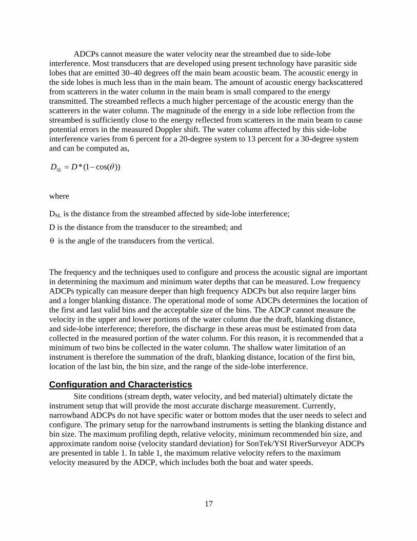
ADCPs cannot measure the water velocity near the streambed due to side-lobe interference. Most transducers that are developed using present technology have parasitic side lobes that are emitted 30–40 degrees off the main beam acoustic beam. The acoustic energy in the side lobes is much less than in the main beam. The amount of acoustic energy backscattered from scatterers in the water column in the main beam is small compared to the energy transmitted. The streambed reflects a much higher percentage of the acoustic energy than the scatterers in the water column. The magnitude of the energy in a side lobe reflection from the streambed is sufficiently close to the energy reflected from scatterers in the main beam to cause potential errors in the measured Doppler shift. The water column affected by this side-lobe interference varies from 6 percent for a 20-degree system to 13 percent for a 30-degree system and can be computed as,

where

DSL is the distance from the streambed affected by side-lobe interference;

D is the distance from the transducer to the streambed; and

θ is the angle of the transducers from the vertical.

The frequency and the techniques used to configure and process the acoustic signal are important in determining the maximum and minimum water depths that can be measured. Low frequency ADCPs typically can measure deeper than high frequency ADCPs but also require larger bins and a longer blanking distance. The operational mode of some ADCPs determines the location of the first and last valid bins and the acceptable size of the bins. The ADCP cannot measure the velocity in the upper and lower portions of the water column due the draft, blanking distance, and side-lobe interference; therefore, the discharge in these areas must be estimated from data collected in the measured portion of the water column. For this reason, it is recommended that a minimum of two bins be collected in the water column. The shallow water limitation of an instrument is therefore the summation of the draft, blanking distance, location of the first bin, location of the last bin, the bin size, and the range of the side-lobe interference.

Configuration and Characteristics Site conditions (stream depth, water velocity, and bed material) ultimately dictate the

instrument setup that will provide the most accurate discharge measurement. Currently, narrowband ADCPs do not have specific water or bottom modes that the user needs to select and configure. The primary setup for the narrowband instruments is setting the blanking distance and bin size. The maximum profiling depth, relative velocity, minimum recommended bin size, and approximate random noise (velocity standard deviation) for SonTek/YSI RiverSurveyor ADCPs are presented in table 1. In table 1, the maximum relative velocity refers to the maximum velocity measured by the ADCP, which includes both the boat and water speeds.

))cos(1(* θ−= DDSL

18

Table 1. Characteristics of SonTek/YSI RiverSurveyor ADCPs [kHz - kilohertz; m – meter; cm – centimeters; s - second] (adapted from SonTek, 2000).

Frequency (kHz)

Maximum Profiling Depth

(m)1

Maximum Relative

Velocity (m/s)

Minimum Recommended Bin Size (cm)

1-Second Standard Deviation

(cm/s) 500 120 10 1 22.2

1,000 40 10 0.25 27.1

1,500 25 10 0.25 20.9

3,000 6 10 0.15 11.7 1 The actual maximum depth that can be profiled depends on the water temperature and sediment in suspension.

Broadband ADCPs manufactured by TRDI offer multiple water and bottom modes. While the multiple water and bottom modes make setup of the instrument more complicated, it also allows the instrument to be optimized for the site conditions. Data collection software for the Rio Grande ADCP from TRDI (TRDI, 2003; 2007) has an automated configuration wizard that optimizes the instrument setup based on the maximum expected velocity, boat speed, water depth, and bed material type.

Water modes offered in Rio Grande ADCPs allow the instrument to be optimized for the water velocity, depth, and bed material present at the time of the measurement. Each water mode has advantages and disadvantages associated with it. Water mode 1 is a robust multipurpose mode that can work in nearly all conditions but the random noise associated with this mode limits the practical application in shallow, low velocity situations. Water modes 5 and 11 are designed for low velocity (less than 1 m/s), shallow water (less than 4 to 8 m, depending on frequency) situations and have specific velocity and depth limitations. The advantage of water modes 5 and 11 are low random errors and small bin sizes. Water mode 12 is a fast ping-rate mode that is similar to water mode 1 but utilizes a faster ping rate and an internal averaging technique of multiple pings per ensemble to reduce the random noise associated with normal mode 1 measurements. This reduction in noise by mode 12 allows smaller bins to be used or lower velocities to be measured efficiently. The heading, pitch, and roll sensors are only measured at the beginning of the averaging interval and bottom track measurements do not occur during the averaging interval, therefore, random instrument movements caused by poor boat operation or turbulent water-surface conditions are unaccounted for in mode 12 and can cause significant errors, if the averaging interval is too long. A maximum averaging interval of 1 second is recommended and this may need to be further reduced in fast turbulent conditions. The maximum profiling depth, the maximum relative velocity, recommended minimum bin size, and random noise for the various water modes available in TRDI Rio Grande ADCPs are summarized in table 2. In table 2, the maximum relative velocity refers to the maximum velocity

19

measured by the ADCP, which includes both the boat and water speeds. The values listed in table 2 for modes 5 and 11 are approximate values. It is possible to collect valid data when the maximum relative velocity is greater than that shown; however this is not necessarily predictable. These values should be used as a guideline to help the user decide whether or not water mode 5 or 11 can be used. The high-resolution pulse-coherent water mode 5 or 11 should be used wherever possible. It is important to also note that not every Rio Grande ADCP has water mode 12; it must be purchased separately and installed on the ADCP. Therefore, a user should check their instrument to determine the available water modes by connecting to the ADCP with a terminal program and issuing a ‘WM?’ command. A more in-depth discussion of the various water modes and their applicability to various site conditions can be found in Appendix C.

Table 2. Characteristics of TRDI Rio Grande water profiling modes for 1,200 kHz and 600 kHz ADCPs [600 kHz values in parentheses; kHz - kilohertz; m – meter; cm – centimeters; s - second] (adapted from TRDI, 2003).

Water Mode

Maximum Depth (m)1

Maximum Relative

Velocity (m/s)

Minimum Recommended Bin Size (cm)

1-Second Standard Deviation

(cm/s) 1 12 (45) 10 (10) 25 (50) 9.5 (9.5)4

5 4 (8)2 0.7 (1)3 5 (10) 0.4 (0.4)4

11 4 (8)2 0.7 (1)3 5 (10) 0.4 (0.4)4

12 12 (45) 10 (10) 5 (10) 18 (18)5 1 The actual maximum depth that can be profiled depends on the water temperature and sediment in suspension. 2 It is possible to profile deeper by decreasing the ambiguity velocity to 3 cm/s (WZ03) but this change reduces the maximum velocity. The WZ03 should be used with caution. 3 The maximum velocity for modes 5 and 11 are highly dependent on depth and turbulence. 4 Assumes a 2-Hz ping rate. 5 Assumes 100 bins and an ambiguity velocity of 1.75 m/s (WV175).

Currently (2007) the broadband ADCPs from TRDI have two bottom modes available. Bottom mode 5 is the general purpose and default water mode, but does not work well in depths below the transducer of less than approximately 0.8 m. Bottom mode 7 uses multiple lags to function in depths as shallow as 0.3 m below the transducer and can function to the full maximum depth of the profiler. The bottom mode 7 multiple lag technique is slower, resulting in less data collected in a fixed time. Therefore, bottom mode 7 is typically used only when bottom mode 5 fails to bottom track.

20

Compass Considerations Most ADCPs reference the water and boat velocity to magnetic north using an internal

fluxgate compass. The effect of compass errors on measurements made with an ADCP is different for water velocity and discharge data depending on the boat velocity reference. When bottom track is used for the boat velocity reference, a compass error will cause a rotational error in the measured water velocity, but the magnitude of the velocity is unaffected. The compass has no effect on measured discharge using bottom track as the boat velocity reference. However, when an external boat velocity reference such as GPS is used, the effect of the compass is significant. Potential errors include errors in the compass reading caused by distortion of the earth’s magnetic field due to objects on the boat, displacement of the compass out of the horizontal position(for example, sudden acceleration or deceleration), and errors in determining the magnetic variation for a specific location. A local magnetic variation can be estimated from available computer models such as Geomagix (http://www.interpex.com/magfield.htm) or GeoMag (http://www.resurgentsoftware.com/GeoMag.html) if the latitude and longitude of the site(s) is known. The magnetic variation can also be determined in the field using techniques described in the WinRiver User’s Guide (TRDI, 2003). When using an external boat velocity reference (such as GPS) compass errors will affect both measured water velocity and discharge. Analytical assessment of the compass errors shows that the effect of these errors on velocity and discharge is directly proportional to the speed of the boat. Therefore, maintaining a boat speed that is slow, steady, and practical for the site conditions is imperative to accurately measuring water velocity and discharge when using an external boat velocity reference.

The accuracy of internal compasses in commercially available ADCPs are typically about

+/- 1-2 degrees. Fluxgate compasses can be unusable when deployed with mounts or boats constructed of ferrous metals or that have significant electrical fields. Use of external heading references can improve the accuracy of the heading measurement and eliminate problems associated with ferrous metals and electrical fields. Traditionally an external heading reference was a gyroscope; however, improvements in GPS technology have made GPS-based heading measurements a cost-effective and accurate solution.

Instrument Quality Assurance Although ADCPs have no moving parts and typically require no calibration, the instruments and associated software and firmware are complex. Quality assurance procedures will help identify potential instrument problems. The procedures discussed do not check all components of the ADCP but will help identify common problems.

Software and Firmware Procedures Upgrades to both software and firmware associated with ADCPs are common. Many of

these upgrades result in minor improvements to the software or firmware and do not substantially affect the quality of discharge measurements made with the instrument. Nevertheless, some software and firmware changes can be major, and can appreciably affect discharge measurement results. Therefore, ADCP users should ensure that the most recent agency-approved software and firmware are used for data collection and processing. Firmware and software revisions should be tested before being used for routine data collection. Testing of software and firmware often requires data collection in a variety of conditions with a variety of ancillary equipment. This can be difficult and time consuming and often requires coordination between select groups of users.

21

In addition to information available from instrument manufacturers, the USGS provides information regarding software and firmware in Technical Memorandums, an open mailing list, and the Office of Surface Water (OSW) Hydroacoustics Web pages at (http://hydroacoustics.usgs.gov/).

Before an ADCP is taken to the field, the most recent agency-approved software should be installed on the primary and any backup field computers. A copy of the software also should be kept on a storage media separate from the field computers, such as a USB (Universal Serial Bus) memory stick, CD-ROM or memory card, in the event of damage or loss of the primary field computer.

Instrument Tests Each ADCP used should be tested: (1) when the ADCP is first acquired; (2) after factory

repair and prior to any data collection; (3) after firmware or hardware upgrades and prior to any data collection; and (4) at some periodic interval (for example, annually). The purpose of an instrument test is to verify that the ADCP is working properly for making accurate discharge measurements. Various methods for testing ADCP accuracy include tow-tank tests, flume tests, and comparing ADCP discharge measurements with discharges from some other source, such as conventional current meters. Each of these methods has limitations as discussed by Oberg (2002).

Beam Alignment Test A common source of instrument bias is for the beams to be misaligned. The user can

evaluate the potential bias caused by beam misalignment by using a simple field test. This test compares the straight-line distance (commonly called the distance made good) measured by bottom tracking to that measured by GPS. Detailed procedures for the beam alignment test are provided in Appendix D. Bottom tracking is known to have a small bias caused by terrain effects but this bias is typically less than 0.2 percent. The USGS recommended criterion is for the ratio of bottom track distance made good to the distance made good measured by a differentially-corrected global positioning system (DGPS) is 0.995 to 1.003 for the ADCP beam alignment to be acceptable. If the instrument does not meet the beam alignment criterion it is recommended that ADCP is returned to the manufacturer and that a custom transformation matrix be determined and loaded into the instrument.

Periodic Instrument Check Periodic instrument checks help ensure consistency among instruments and discharge

measurement techniques. The instrument check may be made at a site where the ADCP-measured discharge can be compared with a known discharge derived from some other source, such as the rating discharge from a site with a stable stage-discharge rating or a concurrent measurement made using an independent technique. If the ADCP is equipped with more than one water- or bottom-tracking mode, it is desirable, though not required, to periodically conduct these tests using the different modes. Periodic instrument checks should be performed at different sites, so that a range of hydrologic conditions are reflected in the tests, and so that any inherent biases associated with a particular site are minimized. The discharge obtained from the ADCP should be within 5 percent of the known discharge, but a consistent bias in the annual records should be investigated. If the comparison reference is a stable stage-discharge rating and

22

the ADCP measurement departs from the rating discharge by more than 5 percent, it is possible that a rating may have shifted. Another measurement with a second ADCP or conventional discharge measurement should be made to check the validity of the rating before drawing definitive conclusions regarding the ADCP instrument test.

Ancillary Equipment Although the ADCP and computer are the primary equipment, the ancillary equipment discussed in this section will help achieve an accurate measurement in a variety of conditions. Not all of the equipment discussed is necessary for every measurement but depending on the site conditions encountered, the appropriate equipment should be available.

GPS Requirements and Specifications Using a GPS to measure the boat velocity is the preferred method of data collection when

moving-bed conditions are present (see Appendix B for details of collecting data in moving-bed conditions). The GPS receiver should support differential corrections, allow real-time data output on a standard RS-232 serial interface, and provide the standard National Marine Electronics Association (NMEA) 0183 (National Marine Electronics Association, 2002) GGA and VTG data strings . The first method for determining the boat velocity from GPS data is to use the velocity of the boat reported in the VTG data string. Typically the velocity reported in the GPS VTG string is determined by the GPS receiver based on measured Doppler shifts in the satellite signals. This velocity measurement can be robust, because it is resistant to some of the errors that are problematic for position determination. Some receivers, particularly low-cost GPS receivers, may apply filters to smooth out the velocity or display a zero velocity when the velocity drops below a specified threshold. These types of filters and thresholds are unacceptable for using the GPS receiver with an ADCP. Use of the Doppler shift to determine velocity does not require and is unaffected by differential corrections.

The second method for determining boat velocity from GPS data is to use the position data in the GGA string and compute velocity from sequential positions by dividing by the time elapsed between position solutions (differentiated position). Use of differentiated position requires accurate position solutions and thus, differential correction. Differential correction compensates for satellite and receiver clock drift, ephemeris inaccuracies, and tropospheric and ionospheric errors associated with the coded signal being broadcast by the GPS satellites and receivers. There are two common methods of differentially correcting a GPS signal, 1) Real-time Kinematic (RTK) systems, which require a user-operated base station (positioned at a known location) and separate rover receiver both of which can receive dual-frequency code-phase and carrier-phase satellite signals, and 2) code-phase differential corrections. RTK systems typically cost tens of thousands of dollars but deliver accuracies in the centimeter range. These systems are used most frequently where satellite-based code-phase corrections are not available or where high-accuracy positions are required. Code-phase differential corrections can be obtained from user-operated base stations but more commonly are obtained from differential correction services. There are two free sources of differential correction services provided by the U.S. Government. The first is the Wide Area Augmentation System (WAAS) developed for the Federal Aviation Administration to provide precision guidance to aircraft at airports and airstrips, using a system of satellites and ground stations that provide GPS signal corrections (Federal Aviation Administration, 2006). The second free source is U.S. Coast Guard radio

23

beacons, which are part of a large network that provides differential correction to coastal areas, navigable rivers, and, more recently, inland agricultural areas. There are commercial satellite differential service providers that provide differential corrections with various levels of accuracy for a fee. These corrections are typically broadcast using a communications satellite. The accuracy of code-phase differential corrects varies by the correction source used and the characteristics of the GPS receiver. Many commercial receivers claim submeter accuracy using WAAS as the differential correction source. These receivers are the most common type of receiver used for ADCP data collection and range in cost from a few hundred dollars to about three thousand dollars.

Experience using GPS with ADCPs has shown the two most common problems are filters in the receiver and multipath errors caused by site conditions. The GPS should allow all filters to be turned off. Multipath errors are caused by the satellite signal reflecting off of bridges, trees, buildings, etc. before arriving at the antenna. Multipath affects only the position solutions; it does not affect Doppler-based GPS velocity data. Some receivers contain special antennas or software to reduce multipath errors. If multipath is a problem during measurements use of VTG is often the best solution.

Echo Sounder Streams with high sediment concentrations of fines and sand being transported on or near

the streambed also may cause inaccuracies in ADCP water-depth measurements, and therefore, an inaccurate discharge. It may be necessary in such conditions to use a lower frequency echo sounder (approximately 200 kHz) to measure the water depth. The echo sounder must be able to support the NMEA 0183 DBT data string to be compatible with ADCP data collection software. If a depth sounder is used, it is important that the echo sounder be properly calibrated as part of the pre-measurement field procedures. For proper calibration techniques, the user is referred to the bar check procedures in the U.S. Army Corps of Engineers, Engineering Design Manual on hydrographic surveying (U.S. Army Corps of Engineers, 2002). The bed-load transport rate or sediment concentration that makes necessary the use of a depth sounder have not been quantified and user judgment is required.

Instrument Deployments and Mounts Every measurement site has unique features that may determine the best type of ADCP

deployment platform. Site features may include hydraulic characteristics such as water velocity and access considerations such as the presence of boat ramps, bridges, or cableways. Three common types of ADCP deployment platforms are manned boats, tethered boats, and remote-control boats. This section discusses the various deployment platforms and associated equipment such as mounts, waterproof enclosures, and radio-modem telemetry.

Manned Boats ADCPs can be mounted on either side of manned boats, off the bow, or in a well through

the hull. Advantages and disadvantages for mounting locations on manned boats are listed in table 3. The ADCP should not be mounted in close proximity to any object containing ferrous metal or sources of strong electromagnetic fields, such as generators, batteries, and boat engines to minimize ADCP compass errors. A good rule of thumb is that an ADCP should not be mounted any closer to a steel object than the largest dimension of that object. This is a rule of

24

thumb, however, and there are large variations in the magnetic fields generated by different metals. Even stainless steel varies appreciably in the amount of ferrous material contained in the steel.

ADCP mounts for manned boats should:

a) allow the ADCP transducers to be positioned free and clear of the boat hull and mount;

b) hold the ADCP in a fixed, vertical position so that the transducers are submerged at all times while minimizing air entrainment under the transducers;

c) allow the user to adjust the ADCP depth easily;

d) be rigid enough to withstand the force of water caused by the combined water and boat speed;

e) be constructed of non-ferrous materials;

f) be adjustable for boat pitch-and-roll; and,

g) be equipped with a safety cable to hold the ADCP in the event of a mount failure.

25

Photographs of a variety of ADCP mounts are available in Simpson (2002, p. 58-69) or on the USGS Hydroacoustics Web pages (http://hydroacoustics.usgs.gov/).

Table 3. Advantages and disadvantages of acoustic Doppler current profiler (ADCP) mounting locations on manned boats (adapted from Oberg and others, 2005).

Mounting Location

Advantages

Disadvantages

Side of boat

Easy to deploy Moderate chance of directional bias in measured discharges with some boats and flows

Mounts are easy to construct and are adaptable to a variety of boats

Possibly closer to ferrous metal (engines) or other sources of electromagnetic fields (EMF)

ADCP draft measurement can be easily obtained

Moderate-low risk of damage to ADCP from debris or obstructions in the water

Susceptible to roll-induced bias in ADCP depths

Bow of boat

Minimizes chance of directional bias in measured discharges

Increased risk of damage to ADCP from debris or obstructions in the water

Mounts relatively easy to construct

More difficult to measure ADCP depth

Usually far from ferrous metal or electromagnetic fields

Susceptible to pitch-induced bias in ADCP depths, particularly at high speeds or during rough conditions (waves)

Well in center of boat

Protected from debris and obstructions

Accurate depth measurements possible

Often requires special modifications to boat

Least susceptible to pitch/roll-induced bias in ADCP depths

26

Tethered Boats A tethered boat can be defined as a small boat (usually less than 2 m long) attached to a

rope or tether, that can be deployed from a bridge, a fixed cableway, or a temporary bank-operated cableway. The tethered boat should be equipped with an ADCP mount that meets all of the specifications outlined in the previous section on manned boats. The tethered boat should also contain a waterproof enclosure capable of housing a power supply and wireless radio modem for data telemetry. A second wireless radio modem attached to the field computer enables communication between the ADCP and field computer without requiring a direct cable connection. The radio modems should reliably communicate with the ADCP using the ADCP data-acquisition software; have a rugged, environmental housing; operate on a 12-volt direct current (DC) power supply; and have at least 38,400 baud data-communication capability to maximize ADCP data throughput (Rehmel and others, 2002). Rehmel and others (2002) describe the development of a prototype tethered platform, a project to refine the platform into a commercially available product, and tethered-platform measurement procedures.

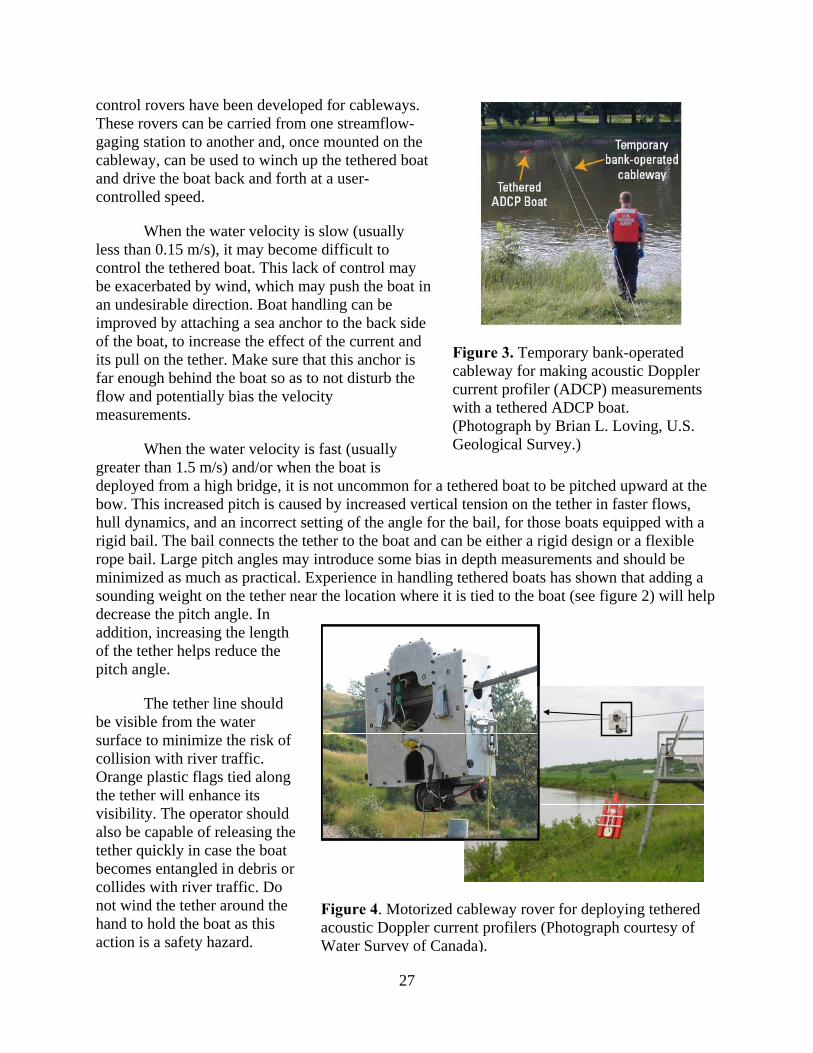
Tethered ADCP boats have become a common deployment method (figure 2). Certain considerations need to be made when making tethered ADCP boat measurements. Tethered boats are used in a variety of settings, but primarily from the downstream side of bridges for convenience. Bridge piers can cause excessive turbulence during high streamflow, especially if debris accumulations are present on the piers and the piers are skewed to the flow. The effect of bridge pier-induced turbulence may be reduced by lengthening the tether to increase the distance between the bridge and the tethered boat. Attention should be paid to the cross section to ensure that there are no large eddies that could cause flow to be non-homogeneous. Possible alternatives to measuring off the downstream side of bridges include bank-operated cableways or having personnel on each bank with a rope attached to the platform, pulling it back and forth across the river. Bank-operated cableways may be as simple as a temporary “rope and pulley” apparatus (figure 3) or may involve the use of a small temporary cableway with a motorized drive for towing the tethered boat back and forth across the stream (figure 4). Recently (2004), remote-

Figure 2. Examples of tethered acoustic Doppler current profiler (ADCP) boats used for making discharge measurements. (Left photograph by Jeff Woodward, Environment Canada and right photograph by Geoffrey D. Cartano, U.S. Geological Survey.)

27

control rovers have been developed for cableways. These rovers can be carried from one streamflow-gaging station to another and, once mounted on the cableway, can be used to winch up the tethered boat and drive the boat back and forth at a user-controlled speed.

When the water velocity is slow (usually less than 0.15 m/s), it may become difficult to control the tethered boat. This lack of control may be exacerbated by wind, which may push the boat in an undesirable direction. Boat handling can be improved by attaching a sea anchor to the back side of the boat, to increase the effect of the current and its pull on the tether. Make sure that this anchor is far enough behind the boat so as to not disturb the flow and potentially bias the velocity measurements.

When the water velocity is fast (usually greater than 1.5 m/s) and/or when the boat is deployed from a high bridge, it is not uncommon for a tethered boat to be pitched upward at the bow. This increased pitch is caused by increased vertical tension on the tether in faster flows, hull dynamics, and an incorrect setting of the angle for the bail, for those boats equipped with a rigid bail. The bail connects the tether to the boat and can be either a rigid design or a flexible rope bail. Large pitch angles may introduce some bias in depth measurements and should be minimized as much as practical. Experience in handling tethered boats has shown that adding a sounding weight on the tether near the location where it is tied to the boat (see figure 2) will help decrease the pitch angle. In addition, increasing the length of the tether helps reduce the pitch angle.

The tether line should be visible from the water surface to minimize the risk of collision with river traffic. Orange plastic flags tied along the tether will enhance its visibility. The operator should also be capable of releasing the tether quickly in case the boat becomes entangled in debris or collides with river traffic. Do not wind the tether around the hand to hold the boat as this action is a safety hazard.

Figure 4. Motorized cableway rover for deploying tethered acoustic Doppler current profilers (Photograph courtesy of Water Survey of Canada).

Figure 3. Temporary bank-operated cableway for making acoustic Doppler current profiler (ADCP) measurements with a tethered ADCP boat. (Photograph by Brian L. Loving, U.S. Geological Survey.)

28

Standard safety practices, site-specific traffic safety plans, and the local highway traffic regulations should be followed.

For tethered boat deployments it is possible to lose control of the boat because of a system component failure. For example, a boat tether or tether attachment point could break. It is recommended that ADCP operators using tethered-boat deployments have redundant attachment points for the tether on the boat and have a contingency plan for retrieving the boat in the event of a failure that causes a loss of boat control. An example of a contingency plan would be to carry a small manned boat that could be quickly and safely launched to retrieve the tethered or remote-control boat (Oberg and others, 2005).

Remote-Control Boats Unmanned, remote-control ADCP boats allow the deployment of ADCPs where

deployment with a manned boat or tethered boat may not be feasible or ideal. Similar to (but smaller than) manned boats, a remote-control boat has self-contained motors and a remote-control system for maneuvering the boat across the river. Unlike the tethered boat, the remote-control boat has no rope (tether) restraints. Although remote-control boats have an increased risk of equipment loss because of potential loss of boat control, they provide the ability to launch a boat without a boat ramp and to collect data away from bridge effects (for example, upstream from a bridge) or at sites where no bridge or cableway is present. Currently remote-control boats are commercially available (figure 5).

A remote-control boat ADCP mount should meet all mount specifications listed for manned boats. The remote-control boat also should contain a waterproof enclosure capable of housing a power supply, a radio modem, and the control radio. Radio modems are used for data telemetry between the remote-control boat and field computer; the radio modems should have the capabilities described for tethered boat deployments.

The same operational guidelines regarding speed and maneuvering for manned boats also apply to remote-control boats. Proper control of a remote-control boat requires practice. The operator should be familiar with remote-control boat operation prior to using this deployment technique in high flows. Regular maintenance of the boat and control radios is critical to ensure

(A) SeaRobotics, Inc. (B) OceanScience Group

Figure 5. Examples of commercially available remote-control boats.

29

reliable operation.

For remote-control boats, it is possible to lose control of the boat because of a system component failure. It is recommended that ADCP operators using remote-control boat deployments have a contingency plan for retrieving the boat in the event of a failure that causes a loss of boat control. An example of a contingency plan would be to carry a small manned boat that could be quickly and safely launched to retrieve the tethered or remote-control boat (Oberg and others, 2005).

Other Equipment New laptop computers typically do not contain a serial port. A serial port is required for

communication with the ADCP and a second serial port is required if a GPS is used. Use of universal serial bus (USB) or Personal Computer Memory Card International Association (PCMCIA) serial ports are often required. USB serial ports are virtual serial ports and some brands to do not work well with ADCPs and/or GPS. Prior to going to the field all ports should be checked for compatibility with the instruments to be used. A list of some USB and PCMCIA serial ports that have been shown to work well for ADCP measurements can be found on the USGS Hydroacoustics Web page (http://hydroacoustics.usgs.gov/).

In addition to the ADCP and computer there is other equipment that is necessary to achieve a high-quality discharge measurement.

• A toolkit should be assembled for the ADCP with tools, multimeter, and any spare parts that may be difficult to obtain in the field (such as fuses, o-rings, and special wrenches). The toolkit should be kept with the ADCP.

• An adequate supply of the agency-approved ADCP discharge-measurement notes should be taken to the field. The USGS discharge-measurement form (9-275-I) is available from the OSW’s Hydroacoustics Web pages (http://hydroacoustics.usgs.gov/) and is shown in Appendix E, figure E-2.

• Computer data-storage media (such as a flash-memory card, USB-memory stick or CD-ROM) with sufficient storage space for making temporary backup copies of all field data files should be available.

• A thermometer is needed to check the accuracy of the ADCP’s water-temperature measurement, as an incorrect temperature will bias the velocity and discharge measurements.

• The depth of the ADCP should be measured. If the ADCP mount does not contain graduated markings, a tape measure or folding rule should be used to make the measurement.

• The distance from the beginning and end of a transect to the nearest edge of water must be measured and input to the software to compute the discharge in the unmeasured areas. Typically visual estimates underestimate the distance over water; therefore, a laser rangefinder or some other means of measuring the

30

distance to shore is required. The calibration of distance-measurement devices should be checked periodically by measuring the distance to targets at a known distance; the results of these tests should be recorded in an office log. Various types of laser and optical rangefinders, accuracy and limitations, and test results can be found on the OSW Hydroacoustics Web pages (http://hydroacoustics.usgs.gov/).

• A conductivity or salinity meter should be used to determine the salinity at the transducer face for measurement in saline environments.

• If the surface velocities are affected by wind, a handheld anemometer should be used to accurately characterize the wind speed and direction.

• If radio modems are utilized for ADCP communications, the cable for connecting directly to the ADCP should be taken to the field. Experience has shown that an ADCP connected through radio modems will occasionally not communicate with the field computer. This problem is often resolved by using a direct cable to establish communications and “reset” the ADCP for modem use. If a second pair of radio modems is available, they should be taken as a backup.

• If low-flow conditions are expected (generally velocities less than 0.15 m/s), a trolling motor or tagline may be necessary to keep boat speed slow and consistent (Oberg and others, 2005). If it is not possible to maintain a slow boat speed, maintain the slowest speed that allows smooth boat operation (additional transects may be necessary to average turbulence and instrument noise).

• If a remote or tethered boat deployment is used, hand-held radios are helpful for communications between the boat operator and the computer operator.

• If the data collection computer will be used in bright sunlight, a shade for the computer screen may be necessary to improve the readability of the screen. In potentially rainy conditions, a rain cover is required to keep non-ruggedized computers dry.

31

A summary listing of this equipment is provided in table 4. An example ADCP field kit that includes some of this equipment is shown in figure 6.

Final Equipment Preparation and Inspection A pre-field inspection checklist is recommended to ensure that all procedures are

followed and that all necessary equipment is available and functioning for the field trip. An example of a pre-field inspection checklist is shown in Appendix E, figure E-1; however the checklist should only be used as a guideline for field preparation. Other equipment may be necessary for the sites and conditions that may be encountered in the field. The ADCP, cables,

Figure 6. Example toolkit of ancillary equipment for use with acoustic Doppler current profilers (ADCPs) when making streamflow measurements. (Photograph by John M. Shelton, U.S. Geological Survey.)

Table 4. List of ancillary equipment to be included in acoustic Doppler current profiler (ADCP) toolkit for use with ADCPs when making streamflow measurements. [USB, Universal Serial Bus; ADCP, acoustic Doppler current profiler]

Equipment Function Optional or Required

USB or PCMCIA serial port(s) Computer connection to ADCP and/or DGPS Optional1

Toolkit Field troubleshooting and repairs. Required

ADCP Field Notes Note keeping Required Computer data-storage media Field backups of data Required

Thermometer Measure water and air temperatures Required

Measuring tape or graduated mount Measure ADCP depth Required Laser rangefinder or other distance measurement tool Measure shore distances Required

Salinity/Conductivity Meter Measure salinity Optional2 Handheld anemometer Obtain estimate of wind speed Optional ADCP cable Direct communication Required Trolling motor or tagline Slow boat speed Optional

Handheld radios Communication during tethered or remote-control boat measurements

Optional

PC Shade/Rain Cover for computer Protection and visual aid for computer Optional

1Required if computer does not support sufficient internal serial ports. 2Required for ADCP measurements in estuaries and coastal streams.

32

connectors, batteries, mounts, and GPS or echo sounders that will be integrated with the ADCP in the field should be inspected for any irregularities. The ADCP should be connected to the field computer, and communications with the ADCP established using the ADCP data-collection software and computer to be used in the field. The ADCP clock should then be set to the appropriate reference time (usually local or Greenwich Mean Time). If radio modems are to be used for communications (tethered and remote-control boat deployments), the communications should be established using the radio modems. If a GPS or echo sounder will be connected to the ADCP in the field, then the GPS and/or echo sounder should be connected with the ADCP to the computer to ensure that they properly function with the ADCP and the ADCP data-collection software. If problems are encountered during any system check, the problems should be resolved by: (1) consulting the necessary technical documentation, (2) calling a qualified agency staff member familiar with ADCPs, (3) calling the vendor technical support unit, or some combination of these three options.

Tethered and remote-control boat hulls, fins, structural members and compartments/hatches should be inspected. The tether line(s) and connectors for a tethered boat should be inspected for wear and to ensure that they are suitable to withstand expected field conditions. When deployed in streams and rivers with high velocities and/or turbulence, redundant attachment points for the tether on the boat should be used to allow the tethered boat to be recovered should the primary attachment point fail. Remote-control boat deployments, motors, servos, and the radio controller should be inspected and tested before going into the field (Oberg and others, 2005).

Figure 6. Example toolkit of ancillary equipment for use with acoustic Doppler current profilers (ADCPs) when making streamflow measurements. (Photograph by John M. Shelton, U.S. Geological Survey.)

33

FIELD PROCEDURES Proper field procedures are critical to high-quality discharge measurement using ADCPs.

A discussion of key aspects of the field procedures are followed by a quick reference sheet that can be used in the field to ensure that all important procedures have been followed. Although step by step procedures are an important aspect of high quality data collection, nothing can substitute for field personnel who understand both the instrument and effect of hydraulic and sediment transport conditions.

Site Selection One of the most important steps in collecting high quality streamflow measurement is site

selection. Many ADCP measurement problems can be solved by moving to a better measurement section. The guidelines in USGS Water-Supply Paper 2175 (Rantz and others, 1982, p. 139) for traditional current meter measurements are also excellent guidelines when using an ADCP, except for those guidelines that relate to depth and velocity requirements for specific meters. General guidelines for selection of an ADCP measurement section can be categorized by location, shape, flow velocity, and other factors.

1. Location:

a. The cross section lies within a straight reach, and streamlines are parallel to each other. Flow is relatively uniform and free of eddies, slack water, and excessive turbulence (Rantz and others, 1982).

b. The measurement section is relatively close to the gaging station control to avoid the effect of tributary inflow between the measurement section and control and to avoid the effect of storage between the measurement section and control during periods of rapidly changing stage (Rantz and others, 1982).

2. Shape:

a. Desirable measurement sections are roughly parabolic, trapezoidal, or rectangular. Asymmetric channel geometries (for example, deep on one side and shallow on the other) should be avoided if possible (Simpson, 2002), as should cross sections with abrupt changes in channel-bottom slope.

b. The streambed cross section should be as uniform as possible and free from debris and vegetation or plant growth.

c. Depth at the measurement site should allow for the measurement of velocity in two or more depth cells at the start and stop points near the left and right edges of water.

3. Flow velocity:

a. Measurement sections with velocities less than 0.09 m/s should be avoided if it is possible to do so, and an alternative measurement location is available. Although measurements can be made in low velocities, boat speeds must be kept extremely

34

slow (if possible, less than or equal to the average water velocity) requiring special techniques for boat control (Simpson, 2002). If it is not possible to maintain a slow boat speed, maintain the slowest speed that allows smooth boat operation (additional transects may be necessary to average turbulence and instrument noise).

b. Sites with very turbulent flow, such as, standing waves, large eddies, and non-uniform flow lines, should be avoided. This condition is often indicative of non-homogenous flow, a condition that violates one of the assumptions required for accurate ADCP velocity and discharge measurements.

4. Other factors:

a. Measurement sections having local magnetic fields that are relatively large as compared to the earth’s magnetic field should be avoided. Large steel structures, such as overhead truss bridges, are a common source for these large local magnetic fields and may result in ADCP compass errors.

b. When using GPS, avoid locations where multipath interference is possible (signals from the satellites bounce off structures and objects such as trees along the bank or nearby bridges or buildings) or where reception of signals from GPS satellites is blocked. It may be possible to make valid measurements in sections that violate one or more of the above guidelines, but whenever possible, locate and use a better measurement section (Oberg and others, 2005).

It is possible that measurements will need to be made where conditions do not satisfy the suggested guidelines. In such situations, the quality of the measurement can be greatly diminished, therefore the field personnel should use their best judgment in selecting a measurement section and making the measurement.

Pre-Measurement Field Procedures A good discharge measurement begins by completing pre-measurement tests and

configuring the instrument properly. The following sections describe the field procedures that should be completed prior to ADCP measurements.

Set Internal Clock Prior to the start of the discharge measurement, the clock internal to the ADCP should be

checked, set to the correct time, and noted on the ADCP measurement field note sheet. This should be done prior to any diagnostic tests, calibrations, or configuration so that time stamps on all data will be consistent. In most cases, the ADCP clock should be set to agree with the recorder time at the streamflow-gaging station. Checking and setting the correct time is of particular importance when using the discharge measurements to calibrate or check the calibration of fixed acoustic current meters installed at streamflow-gaging stations, or when measuring at sites where the flow is unsteady (Oberg and others, 2005).

35

Instrument Diagnostic Checks After the ADCP is mounted and communication between the ADCP and field computer

is established, the instrument must be checked to ensure all components are operating properly. Instrument diagnostic tests should be performed and the results electronically stored on the field computer. Diagnostic tests should include system serial number, firmware and hardware configuration versions, the beam transformation matrix, electronics diagnostic tests, internal system tests, and sensor verification tests. Software for executing diagnostic tests for some ADCPs is available on the USGS Hydroacoustics Web pages and/or is built into the data collection software available from the manufacturer. If software or diagnostic test information is not available for a specific instrument, the user should contact the manufacturer for guidance. The results of diagnostic tests should be backed up in the field and archived in the office with the associated discharge measurement files. Diagnostics tests should be documented on the ADCP discharge-measurement note form (Appendix E, figure E-2). It is recommended that complete diagnostic tests be made prior to every discharge measurement. It is usually prudent to conduct the test from a stationary boat in relatively still water, for example, near the shore. Some of the tests conducted require little or no water motion relative to the ADCP.

Speed of Sound Variation in the speed of sound with depth does not effect the measurement of horizontal currents (Teledyne RD Instruments, 1996); however, it does effect the measurement of vertical currents and the depth (range from the transducer). Regarding horizontal velocity measurements, Snell’s law says the horizontal wave number is conserved when sound passes through horizontal interfaces. Because the frequency of the sound wave remains constant, the change in speed of sound with depth does not effect the horizontal component of the sound velocity and hence the horizontal velocity measurement. The measurement of the vertical velocity component and the depth is proportional to the change in speed of sound. Currently (2007), commercially available data collection and processing software do not have the capability for correcting the vertical velocity or the depth for changes in the speed of sound. Temperature and salinity are the two most important variables for determining the speed of sound for boat-mounted ADCPs.

Water Temperature ADCPs have built-in temperature sensors to measure water temperature at the transducer

face. The ADCP must compute the speed of sound correctly to accurately measure velocities, depths, and compute discharge. Temperature is the most important term in the equation used to compute the speed of sound (Urick, 1983, p. 113). An error of 5° C in the temperature measurement will cause a 2 percent bias error in the measured discharge. Thus, the temperature measured by the ADCP should be compared with an independent temperature measurement made adjacent to the ADCP. This check should be performed prior to every discharge measurement and the results recorded on the measurement field note sheet. If the temperature measured by the ADCP temperature sensor differs consistently from the independent temperature measurement by 2° C or more, or if the ADCP temperature sensor has failed, the ADCP should not be used to make discharge measurements until the temperature sensor is repaired and checked. In the event that a discharge measurement is necessary and another ADCP is not readily available, it may be possible to enter a temperature manually for use in the speed of sound calculations. This action is not recommended as standard practice, however, and it may decrease the accuracy of the discharge measurement.

36

Salinity Salinity is another important term in the speed of sound equation. Salinity values

generally range from 0 parts per thousand (ppt) for freshwater to 35 ppt for water from the open ocean. When measuring in waters where the salinity is greater than zero, the salinity should be measured near the transducer face and recorded on the field note sheet. The salinity value may then be entered into the ADCP data-collection software prior to data collection and adjusted as necessary during playback and processing. Salinity should be measured for every transect in locations where salinity varies over time. Salinity may also vary from bank to bank. It should be noted that the salinity value used for that transect should reflect an average salinity for the section to be measured at the approximate depth of the ADCP transducers.

Compass Calibration Calibrating the internal magnetic compass is encouraged for all ADCP measurements, but is

mandatory when using GPS as the navigation reference, using the loop method for correcting discharge for bias caused by a moving bed (Mueller and Wagner, 2006), or when the velocity direction is important . The instrument-specific procedures available from the manufacturer for calibrating the compass of the ADCP being used should be followed. An automated program from some ADCPs is available on the USGS Hydroacoustics Web pages (http://hydroacoustics.usgs.gov/). The following guidelines should be followed for successful compass calibrations:

1. Minimize ferrous material located in the vicinity of the ADCP. Ferrous material may adversely affect the performance of the internal magnetic compass.

2. If the instrument calibration or evaluation process reports a total compass error, this error should be less than 1 degree when evaluated after calibration. If the error exceeds 1 degree, the calibration procedure should be repeated. If after several attempts, the total compass error cannot be reduced to less than 1 degree, the compass error should be noted on the field sheet. The discharge measurement can then be made, but special attention should be paid to potential compass errors (for example, directional bias and irregular ship track). If the instrument does not report a numerical error, the instrument should report an “excellent” rating for the horizontal calibration parameter.

3. Pitch-and-roll changes must be minimized with Rio Grande ADCPs as they are equipped only for a single-tilt calibration process. In such situations, the standard deviation of the pitch-and-roll should be less than 1 degree, and, ideally, 0.5 degree or less, during the calibration and evaluation process. For RiverSurveyors, pitching and rolling the instrument is encouraged during the calibration, but only the rating of the horizontal calibration is of major concern.

4. Compass calibration should be done as close to the measurement site as possible with the ADCP mounted in the same manner as it will be deployed for the measurement.

5. For best results, maximum rotation velocity should be 5 degrees per second or less.

37

Instrument Configuration The ADCP should be configured by a trained user to reflect the hydrologic conditions at

the site and to optimize the data quality (Lipscomb, 1995). ADCP configuration parameters that must be set include the blanking distance, water mode (if applicable), depth cell (bin) size, and profiling range. Other parameters that should be set prior to data collection but can be modified during postprocessing include the instrument draft, edge shape, top and bottom extrapolation method, and magnetic variation. Configuration parameters are specific to the kind of ADCP being used (narrowband or broadband) and the manufacturer and model. For a detailed description of all configuration parameters the reader should refer to the technical documentation for their specific instrument. General recommendations for configuration parameters are given below.

1. File names for the data files collected (also called deployment names) should follow a uniform, documented convention developed by each agency involved in ADCP operation.

2. The depth of the ADCP (vertical distance from the water surface to the center of the transducer faces) must be measured accurately, recorded in the ADCP discharge-measurement notes, and entered into the configuration file. The pitch-and-roll of the boat when the depth is measured should be similar to the pitch-and-roll during the discharge measurement. If the depth of the ADCP changes during the measurement, the depth must be re-measured, noted, and the configuration file modified with the new depth.

3. Most ADCP data-collection software contains an automated method to configure the ADCP. The automated methods are dependent upon user-supplied information about site characteristics, such as maximum water depth, bed-material characteristics, and expected maximum water and boat speeds. Where these methods are available in ADCP data-collection software, it should be used to configure the ADCP for discharge measurements (U.S. Geological Survey, 2003). The commands generated by this software utility, however, should be checked prior to the start of the measurement.

4. The configuration parameters and/or the site conditions entered into an automated configuration program should be documented in the field notes. Changes made to the ADCP configuration during a measurement should be documented on the measurement field note sheets, so it is clear that changes were made and to which transects these changes apply.

5. Manual configuration of an ADCP should only be used in rare cases where the automated procedures are not applicable. The most up-to-date agency specific guidelines for the instrument should be understood before attempting a manual configuration. If guidelines are not available, the user should use manufacturer recommendations for the unit. It is advisable, however, to seek advice from acoustic experts within the user’s agency.

6. Configuration of the ADCP to collect single-ping water data is preferable, if random noise levels do not prohibit this configuration. Collection of single-ping data allows possible data-quality problems to be more easily identified than multi-ping averaged data. When collecting multi-ping averaged data, the user should be aware of how often the

38

heading, pitch, and roll sensors are sampled and how often water depth and boat velocity are measured. Typically this is done automatically in most narrowband ADCPs but the flexibility provided by water mode 12 in Broadband ADCPs allows the user to set a configuration that is not optimal for moving-boat deployments. If the averaging interval is too long for the boat stability and water turbulence, errors can be introduced into the measurement.

7. The extrapolation method for the top and bottom unmeasured zones must be specified. Often, the appropriate extrapolation method cannot be determined until after the measurement, during post-processing. Experience with previous data collected at a site may be used to guide the selection of the extrapolation method. In the absence of any other information, the one-sixth (0.1667 power coefficient) power-law extrapolation method is a good assumption for most steady-flow sites. The extrapolation methods should be evaluated and, if necessary, changed during post-processing.

8. Wind speed can be important, especially for sites with slow velocities where wind can greatly affect the surface velocities and influence the top extrapolation method to be applied. Overall wind speed and direction as well as changes between transects, should be noted on all measurement field note sheets to assist in accurately processing and reviewing measurements.

9. If the user is unfamiliar with the measurement section a trial transect, which may or may not be recorded, should be made across the river. Information gleaned from the trial transect should be recorded on the discharge-measurement notes. A trial transect is useful for determining the following characteristics of the proposed measurement section:

a. maximum water depth;

b. overall cross-section shape;

c. maximum water velocity and its location in the cross section;

d. flow uniformity;

e. effects of hydraulic structures, such as bridges, piers, islands on the flow;

f. unusual flow conditions such as reverse or bi-directional flow;

g. bank shapes; and

h. approximate start-and-stop locations on the left and right banks, where a minimum of two depth cells with valid velocity measurements can be measured.

10. Buoys can be used for marking the start and stop points in order to aid in obtaining consistent edge estimates, but are not required.

39

Moving-Bed Tests ADCPs can measure the boat velocity using a technique called bottom tracking, which

computes the Doppler shift of acoustic pulses reflected from the streambed. This technique assumes that the streambed is stationary; however, sediment transport on or near the streambed can affect the Doppler shift of the bottom-tracking pulses. In such situations, reflections of bottom-tracking pulses from highly concentrated near-bed sediments contaminate the reflections from the bed. These near-bed sediments are typically being transported in the downstream direction. If bottom tracking is affected by sediment transport, the measured boat velocity will be biased in the opposite direction of the sediment movement. A stationary boat in the stream would appear to be moving upstream (figure 7). This bias in the boat velocity will result in measured velocities and discharge that are less than the true velocities and discharge (negative bias).

USGS policy (U.S. Geological Survey, 2002b) requires that a moving-bed test be made prior to making a discharge measurement. However, it may not be necessary to do a moving-bed test for every discharge measurement, if it can be documented from previous measurements that moving-bed tests are not necessary on a site-by-site basis, either because there is no moving bed or there is always a moving bed. Documentation must contain moving-bed tests for the range of expected flows at the site. If a site has been documented as routinely having a moving bed, periodic moving-bed tests should be made at low flows to verify that GPS is still needed because bottom-track measurements are typically less prone to errors. Sediment transport characteristics can vary greatly for the same discharge, depending on the hydrograph shape, source of runoff,

-100 -80 -60 -40 -20 0 20-10

0

10

20

30

40

50

60

70

DISTANCE IN EAST DIRECTION IN METERS

DIST

ANCE

INNO

RTH

DIRE

CTIO

NIN

SHIP TRACKFLOW DIRECTION

START

END

ME

TER

S

Figure 7. Example of a moving bed measured with a 1,200-kilohertz acoustic Doppler current profiler (ADCP) on the

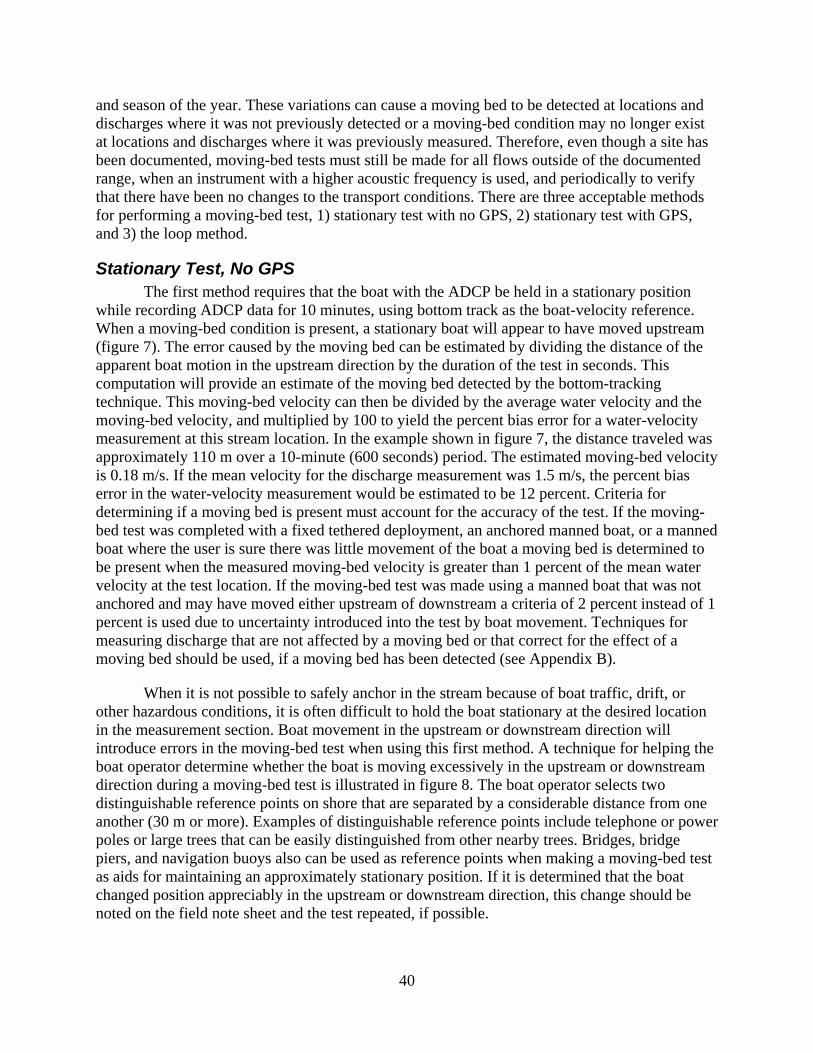
40

and season of the year. These variations can cause a moving bed to be detected at locations and discharges where it was not previously detected or a moving-bed condition may no longer exist at locations and discharges where it was previously measured. Therefore, even though a site has been documented, moving-bed tests must still be made for all flows outside of the documented range, when an instrument with a higher acoustic frequency is used, and periodically to verify that there have been no changes to the transport conditions. There are three acceptable methods for performing a moving-bed test, 1) stationary test with no GPS, 2) stationary test with GPS, and 3) the loop method.

Stationary Test, No GPS The first method requires that the boat with the ADCP be held in a stationary position

while recording ADCP data for 10 minutes, using bottom track as the boat-velocity reference. When a moving-bed condition is present, a stationary boat will appear to have moved upstream (figure 7). The error caused by the moving bed can be estimated by dividing the distance of the apparent boat motion in the upstream direction by the duration of the test in seconds. This computation will provide an estimate of the moving bed detected by the bottom-tracking technique. This moving-bed velocity can then be divided by the average water velocity and the moving-bed velocity, and multiplied by 100 to yield the percent bias error for a water-velocity measurement at this stream location. In the example shown in figure 7, the distance traveled was approximately 110 m over a 10-minute (600 seconds) period. The estimated moving-bed velocity is 0.18 m/s. If the mean velocity for the discharge measurement was 1.5 m/s, the percent bias error in the water-velocity measurement would be estimated to be 12 percent. Criteria for determining if a moving bed is present must account for the accuracy of the test. If the moving-bed test was completed with a fixed tethered deployment, an anchored manned boat, or a manned boat where the user is sure there was little movement of the boat a moving bed is determined to be present when the measured moving-bed velocity is greater than 1 percent of the mean water velocity at the test location. If the moving-bed test was made using a manned boat that was not anchored and may have moved either upstream of downstream a criteria of 2 percent instead of 1 percent is used due to uncertainty introduced into the test by boat movement. Techniques for measuring discharge that are not affected by a moving bed or that correct for the effect of a moving bed should be used, if a moving bed has been detected (see Appendix B).

When it is not possible to safely anchor in the stream because of boat traffic, drift, or other hazardous conditions, it is often difficult to hold the boat stationary at the desired location in the measurement section. Boat movement in the upstream or downstream direction will introduce errors in the moving-bed test when using this first method. A technique for helping the boat operator determine whether the boat is moving excessively in the upstream or downstream direction during a moving-bed test is illustrated in figure 8. The boat operator selects two distinguishable reference points on shore that are separated by a considerable distance from one another (30 m or more). Examples of distinguishable reference points include telephone or power poles or large trees that can be easily distinguished from other nearby trees. Bridges, bridge piers, and navigation buoys also can be used as reference points when making a moving-bed test as aids for maintaining an approximately stationary position. If it is determined that the boat changed position appreciably in the upstream or downstream direction, this change should be noted on the field note sheet and the test repeated, if possible.

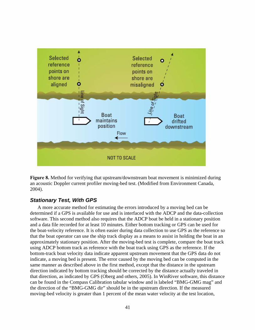
41

Figure 8. Method for verifying that upstream/downstream boat movement is minimized during an acoustic Doppler current profiler moving-bed test. (Modified from Environment Canada, 2004).

Stationary Test, With GPS A more accurate method for estimating the errors introduced by a moving bed can be

determined if a GPS is available for use and is interfaced with the ADCP and the data-collection software. This second method also requires that the ADCP boat be held in a stationary position and a data file recorded for at least 10 minutes. Either bottom tracking or GPS can be used for the boat-velocity reference. It is often easier during data collection to use GPS as the reference so that the boat operator can use the ship track display as a means to assist in holding the boat in an approximately stationary position. After the moving-bed test is complete, compare the boat track using ADCP bottom track as reference with the boat track using GPS as the reference. If the bottom-track boat velocity data indicate apparent upstream movement that the GPS data do not indicate, a moving bed is present. The error caused by the moving bed can be computed in the same manner as described above in the first method, except that the distance in the upstream direction indicated by bottom tracking should be corrected by the distance actually traveled in that direction, as indicated by GPS (Oberg and others, 2005). In WinRiver software, this distance can be found in the Compass Calibration tabular window and is labeled “BMG-GMG mag” and the direction of the “BMG-GMG dir” should be in the upstream direction. If the measured moving-bed velocity is greater than 1 percent of the mean water velocity at the test location,

42

techniques for measuring discharge that are not affected by a moving bed or that correct for the effect of a moving bed should be used (see Appendix B).

Loop Test Stationary moving-bed tests, assuming the ADCP can be held stationary, are a good measure of the magnitude of an apparent moving streambed; however, these tests represent only one location in the cross section, are time consuming, and do not provide a direct means of correcting a biased discharge measurement. An alternative to the stationary moving-bed test is the loop method, which is based on the fact that as an ADCP is moved across the stream, a moving bed will cause the bottom track-based ship track to be distorted in the upstream direction. Therefore, if an ADCP makes a two-way crossing of a stream (loop) with a moving bed and returns to the exact starting position, the bottom track-based ship track will show that the ADCP will have returned to a position upstream from the original starting position (figure 9). The mean moving-bed velocity can be estimated from the distance the ADCP appeared to have moved upstream from the starting position (loop-closure error) and the time required completing the loop.

TD

V upmb = ,

where

mbV is the mean moving-bed velocity for the measurement section,

Dup is the loop-closure error (distance made good, straight-line distance from starting point to ending point), and

T is the measurement time required to complete the loop.

These data are readily available from most commercial software used to measure discharge with ADCPs (figure 10).

43

-100 -50 0 50 100 150

-250

-200

-150

-100

-50

0

50

Distance East in m

Dis

tanc

e N

orth

in m

Dup = Apparent Distance Moved Upstream

Distance east in meters

Dis

tanc

e no

rth in

met

ers

-100 -50 0 50 100 150

-250

-200

-150

-100

-50

0

50

Distance East in m

Dis

tanc

e N

orth

in m



Dis

tanc

e no

rth in

met

ers

Figure 9. Example of the distorted ship track in a loop caused by a moving bed.

Dup

TVmb =

(A) (B)

Dup

TVmb =

Dup

TVmb =

(A) (B)

Figure 10. Example of parameters used to compute the mean correction for data collected with an ADCP and displayed with (A) WinRiver and (B) RiverSurveyor.

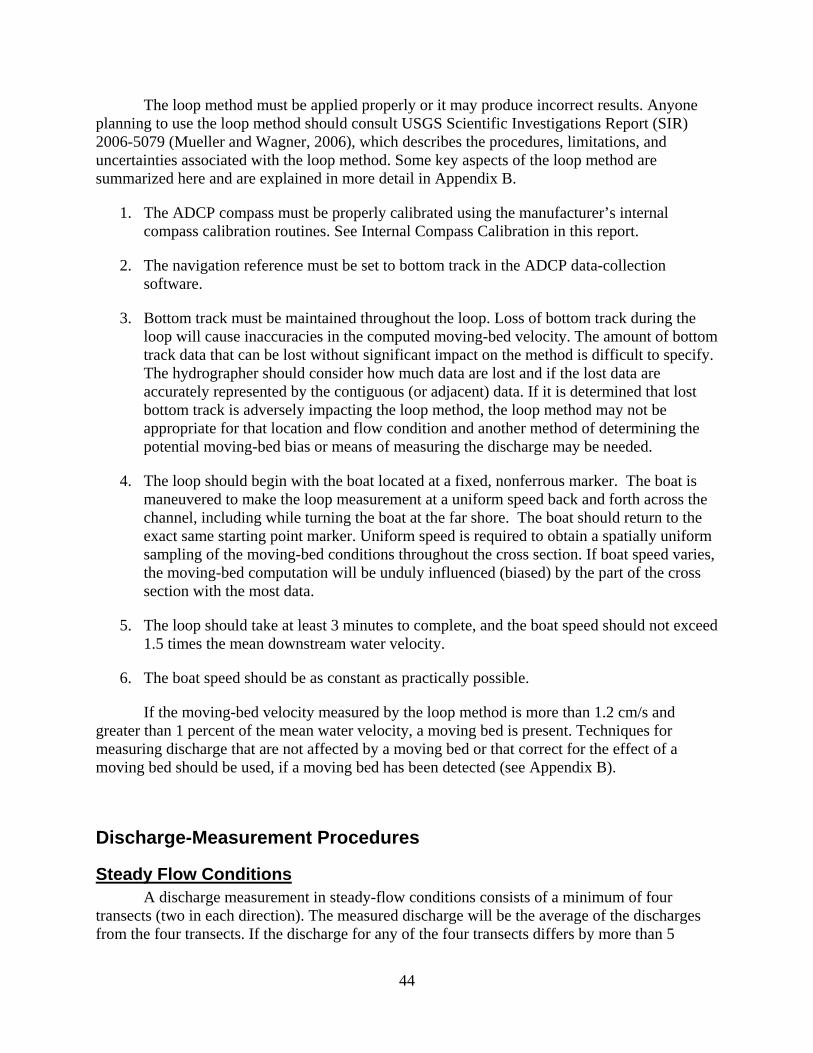
44

The loop method must be applied properly or it may produce incorrect results. Anyone planning to use the loop method should consult USGS Scientific Investigations Report (SIR) 2006-5079 (Mueller and Wagner, 2006), which describes the procedures, limitations, and uncertainties associated with the loop method. Some key aspects of the loop method are summarized here and are explained in more detail in Appendix B.

1. The ADCP compass must be properly calibrated using the manufacturer’s internal compass calibration routines. See Internal Compass Calibration in this report.

2. The navigation reference must be set to bottom track in the ADCP data-collection software.

3. Bottom track must be maintained throughout the loop. Loss of bottom track during the loop will cause inaccuracies in the computed moving-bed velocity. The amount of bottom track data that can be lost without significant impact on the method is difficult to specify. The hydrographer should consider how much data are lost and if the lost data are accurately represented by the contiguous (or adjacent) data. If it is determined that lost bottom track is adversely impacting the loop method, the loop method may not be appropriate for that location and flow condition and another method of determining the potential moving-bed bias or means of measuring the discharge may be needed.

4. The loop should begin with the boat located at a fixed, nonferrous marker. The boat is maneuvered to make the loop measurement at a uniform speed back and forth across the channel, including while turning the boat at the far shore. The boat should return to the exact same starting point marker. Uniform speed is required to obtain a spatially uniform sampling of the moving-bed conditions throughout the cross section. If boat speed varies, the moving-bed computation will be unduly influenced (biased) by the part of the cross section with the most data.

5. The loop should take at least 3 minutes to complete, and the boat speed should not exceed 1.5 times the mean downstream water velocity.

6. The boat speed should be as constant as practically possible.

If the moving-bed velocity measured by the loop method is more than 1.2 cm/s and greater than 1 percent of the mean water velocity, a moving bed is present. Techniques for measuring discharge that are not affected by a moving bed or that correct for the effect of a moving bed should be used, if a moving bed has been detected (see Appendix B).

Discharge-Measurement Procedures

Steady Flow Conditions A discharge measurement in steady-flow conditions consists of a minimum of four

transects (two in each direction). The measured discharge will be the average of the discharges from the four transects. If the discharge for any of the four transects differs by more than 5

45

percent from the measured discharge, and there is no critical data-quality problem that can be identified and documented, a minimum of four additional transects should be obtained and the average of all eight transects will be the measured discharge (U.S. Geological Survey, 2002b). If the discharge for one or more transects is not within 5 percent of the average and there is a critical data-quality problem that can be identified and documented (for example, a tow boat approaching the section, a sudden change in discharge because of a lockage, appreciable data lost because of computer problems, and other factors), the transect deviating from the mean may be replaced with an additional transect in the same direction. Reciprocal transects should always be made to reduce potential directional biases. Directional biases occur when the discharges measured for transects from the left bank to the right bank are consistently either greater than or less than discharges measured for transects made from the right bank to the left bank.

Unsteady Flow Conditions Measurements in conditions where the flow is changing rapidly enough where four

transects within 5 percent of the mean cannot be collected present special considerations. Unsteady flows can be caused by upstream dam or lock regulation, tidal effects, downstream backwater effects, flood waves, or other conditions. It may be necessary to use individual transects as discrete measurements of discharge, if the flow is changing rapidly. If possible, however, pairs of reciprocal transects should be averaged together as one measurement of discharge to reduce the potential of directional bias (U.S. Geological Survey, 2002b). The justification for using a single transect or pairs of transects for discharge measurements should be documented in the field notes and stored with the discharge measurement or applicable station analysis files. Another consideration for unsteady flows, specifically bi-directional flows, is the assignment of a positive or negative sign to the discharge measurement. The ADCP software may or may not assign flow direction correctly and the sign also can depend on which edge is designated “left” or “right;” thus, the operator should note the direction of flow during each transect, according to accepted convention for a particular site.

Critical Data-Quality Problems When making ADCP discharge measurements, the ADCP operator should continuously

monitor the data through the ADCP software. If a critical data-quality problem is observed during a transect, the transect may be terminated. If a transect is terminated, the reason should be documented on the ADCP discharge-measurement field note sheet. The discharge from that transect should not be used in the computation of measurement discharge. If the problem was related to undesirable measurement section characteristics, a new measurement section should be located and noted on the measurement field note sheet. If the terminated transect was not the first transect in a measurement series, the boat should be returned to the initial starting point to ensure the transects are run in reciprocal pairs. (Oberg and others, 2005). Potential critical data-quality problems can include:

a) inappropriate or improperly configured water or bottom mode;

b) configuration errors such as an insufficient number of depth cells to profile to the channel bed;

c) appreciable and/or consistent portion of the section with invalid or missing data;

46

d) appreciable lost bottom track;

e) erroneous boat or water velocities, such as ambiguity errors (see Appendix A);

f) excessive boat speed;

g) poor GPS data attributed to multipath, satellite changes, high DOP, etc.;

h) excessive pitch and roll or erratic motion of boat and ADCP; and,

i) inadvertent early termination of the transect.

Boat Operation Average boat speed for each transect normally should be less than or equal to the average

water speed. At some sites, it may be necessary to move the boat across the channel using a non-ferrous tag line in order to meet this requirement. Other methods for moving the boat slow enough to be equal to or less than the water speed include the use of push poles, paddles, low-speed trolling motors, or tethered boats (a tethered boat deployed from a hand-operated cableway or bridge can be moved slowly across the channel). In certain conditions, it may not be possible to keep the boat speed less than the water speed. If it is not practical or safe to keep the boat speed less than or equal to the average water speed, additional transects may be made to obtain a good average discharge. The reason for maintaining a boat speed that is higher than the average water speed should be documented on the ADCP measurement field note sheet. Ongoing research (Oberg and Mueller, 2007) indicates that the number of passes and the boat speed is not as important as the cumulative time in which data are collected and averaged. A cumulative time for data collection of at least 720 seconds should result in a good mean discharge in steady flow conditions. When using GPS, it is especially important to keep the boat speed as low as practical because errors in the compass readings are additive and increase with boat speed. Rapid boat course changes should be avoided; the key element in boat operation during the measurement is to do everything slowly and smoothly. Simpson (2002) discusses proper boat operation for ADCP measurements in detail. His remarks on boat operation should be heeded (Simpson, 2002, p. 122).

“Be a smooth operator! The BB-ADCP discharge-measurement system will give more consistent results if rapid movements and course changes are kept to a minimum. Smooth boat motion is more important than a straight-line course.”

47

Estimating Edge Discharge Because depths will eventually get too shallow for valid data collection as the ADCP

approaches a bank, it is necessary to estimate discharge in the near-shore unmeasured zones using the ADCP discharge-measurement software. In order to ensure the accuracy of near-shore discharge estimates, the distances from the edge of water to the starting and stopping point of each transect should be measured using a distance-measurement device (such as a laser or optical rangefinder), tagline, or some other accurate measurement device. Placing marker buoys at the start and end points of transects is advantageous for keeping consistent edges. Use of marker buoys enhances the data collection by ensuring more consistent edge estimates and by measuring in approximately the same section for all passes. When measuring in channels with vertical walls at the edges, start and stop points for transects should be no closer to the wall than the depth of water at the wall to prevent acoustic interference from the main beam or side lobes impinging on the wall. For example, if the depth at a vertical wall is 10 m, transects should start/stop at least 10 m away from the wall. In order to obtain an accurate mean velocity for estimating the discharge in the near-shore zones, the boat should be held nearly stationary from 5 to 10 seconds at the beginning and end of each transect. Accurate edge discharge estimates also require the ADCP operator to select the correct edge-shape coefficient for the type of edge (sloping or vertical). The edge shapes should be recorded on the ADCP discharge-measurement notes (Oberg and others, 2005).

When using a tethered boat, special methods are required to measure edge distances. Distance marks on the bridge handrail or guardrail may be used to measure edge distances (figure 11). If the tethered boat is too far away from the bridge to accurately use distance marks for measuring edge distances, laser rangefinders having a compass and inclinometer and a “missing line mode” capability may be used. Missing line mode calculates a horizontal distance between two points, given a range, heading, and vertical angle measured for each point. Edge distance may be measured by selecting the shore and the transect start or end point while using this mode (Rehmel and others, 2002).

When using a remote-control boat at some sites, edge distances may be measured using the same techniques as with tethered boats. At other sites where edge distances cannot be measured using these techniques, it may be necessary to have someone in line with the measurement section to measure the distance from the near-shore edge of water to the starting point and the distance from the ending point to the edge of water on the far shore.

Figure 11. Measuring edge distances when using a tethered acoustic Doppler current profiler boat for discharge measurements (modified from Environment Canada, 2004).

48

Field Notes All information on an ADCP measurement field note sheets should be filled out in the

course of the measurement. The ADCP operator should note any conditions that potentially could affect the measurement, including estimated wind speed and direction, bi-directional or unusual flow patterns, excessive waves, or passing boats. Use of an ADCP does not negate long-standing, agency guidelines and policies regarding measurement documentation, such as recording reference gage heights before, after, and, if needed, during the discharge measurement. An example of a completed USGS ADCP discharge measurement field note sheet is shown in figure 12 (Oberg and others, 2005).

Step by Step Procedure A field form detailing the step by step procedure for making ADCP discharge

measurements is presented in Appendix E, figure E-3.

Post-Measurement Field Procedures An assessment of the discharge measurement should be made after completion of the

transects comprising the measurement. A thorough review of all measurement data may not be practical in the field, but a cursory review of the measurement should be made in order to assign

Figure 12. Example of completed acoustic Doppler current profiler discharge-measurement field note sheets (Oberg and others, 2005).

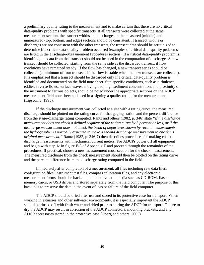
49

a preliminary quality rating to the measurement and to make certain that there are no critical data-quality problems with specific transects. If all transects were collected at the same measurement section, the transect widths and discharges in the measured (middle) and unmeasured (top, bottom, and edge) sections should be consistent. If transect widths or discharges are not consistent with the other transects, the transect data should be scrutinized to determine if a critical data-quality problem occurred (examples of critical data-quality problems are listed in the Discharge-Measurement Procedures section). If a critical data-quality problem is identified, the data from that transect should not be used in the computation of discharge. A new transect should be collected, starting from the same side as the discarded transect, if flow conditions have remained steady. If the flow has changed, a new transect series should be collected (a minimum of four transects if the flow is stable when the new transects are collected). It is emphasized that a transect should be discarded only if a critical data-quality problem is identified and documented on the field note sheet. Site-specific conditions, such as turbulence, eddies, reverse flows, surface waves, moving bed, high sediment concentration, and proximity of the instrument to ferrous objects, should be noted under the appropriate sections on the ADCP measurement field note sheet and used in assigning a quality rating for the measurement (Lipscomb, 1995).

If the discharge measurement was collected at a site with a rating curve, the measured discharge should be plotted on the rating curve for that gaging station and the percent difference from the stage-discharge rating computed. Rantz and others (1982, p. 346) state “If the discharge measurement does not check a defined segment of the rating curve by 5 percent or less, or if the discharge measurement does not check the trend of departures shown by recent measurements, the hydrographer is normally expected to make a second discharge measurement to check his original measurement.” Rantz (1982, p. 346-7) then describes procedures for making check discharge measurements with mechanical current meters. For ADCPs power off all equipment and begin with step 1c in figure E-3 of Appendix E and proceed through the remainder of the procedures. If practical, choose a new measurement cross section for the check measurement. The measured discharge from the check measurement should then be plotted on the rating curve and the percent difference from the discharge rating computed in the field.

Immediately after completion of a measurement, all files including raw data files, configuration files, instrument test files, compass calibration files, and any electronic measurement forms should be backed up on a nonvolatile media such as CD-ROM, flash-memory cards, or USB drives and stored separately from the field computer. The purpose of this backup is to preserve the data in the event of loss or failure of the field computer.

The ADCP should be dried after use and stored in its protective case for transport. When working in estuaries and other saltwater environments, it is especially important the ADCP should be rinsed off with fresh water and dried prior to storing the ADCP for transport. Failure to dry the ADCP may result in corrosion of the ADCP connectors, mounting brackets, and any ADCP accessories stored in the protective case (Oberg and others, 2005).

50

OFFICE PROCEDURES Upon return to the office from field data collection, routine maintenance of equipment

should be completed, all data files and notes should be stored properly, data should be reviewed, and measurements should be finalized and archived. Adherence to these procedures will ensure the equipment is ready for the next deployment and that data are reviewed and processed in the most efficient manner.

Preventative Maintenance The ADCP and associated accessories (DGPS, vertical depth sounders, and electronic

rangefinders) should be inspected upon return from the field to determine their condition. Deployment platforms and mounts also should be inspected. Damage or undue wear to any instrument components, deployment platforms, or mounts should be corrected as soon as possible. The ADCP, all accessories, platforms, mounts, and field computers should be prepared for redeployment and stored in an appropriate location. All batteries should be recharged immediately to facilitate rapid reuse.

Data Storage All measurement files should be moved from the field computer or field backup media to

a permanent storage location for archival and backup. Field computers used to collect ADCP data should have local area network (LAN) capability to facilitate the process of transferring the measurement data to an office server. Measurement Review Procedures

Discharge measurements should be reviewed in detail by the person that made the measurements as soon as practical after completion of ADCP field measurements. ADCP discharge measurements should be routinely checked by someone other than the person who made the measurement, in accordance to specific agency policies.

Important aspects of reviewing ADCP discharge-measurements both in the office and in the field as the data are collected are listed below.

1. The discharge-measurement field note sheets should be complete, clear, and legible.

2. All electronic data files associated with the measurement should be backed up in the field and archived on an office server.

3. The number of transects collected should be appropriate for the flow conditions and satisfy agency policy. Transects should be collected in reciprocal pairs.

4. Configuration files should be checked for errors, appropriateness for the hydrologic conditions, and for consistency with field notes. ADCP depth, salinity, edge distances, edge shapes, extrapolation methods, and ADCP configuration parameters shown on the field notes should match those in the configuration file.

5. The temperature measured by the ADCP thermistor should be reasonable for the site and time of year and match the water temperature measured and noted on the field sheet. Speed-

51

of-sound calculations that are not corrected for temperature can cause velocity measurement errors and depth errors as great as 7 percent. An error in temperature caused by a faulty ADCP thermistor results in an erroneous calculation of water density and introduces uncertainty into the speed-of-sound calculations (Simpson, 2002).

6. The salinity of the water at the measurement site should be measured and noted on the field

sheet and entered into the ADCP software for use in the speed-of-sound calculations. If the hydrographer has entered an incorrect salinity value or has forgotten to enter the proper value, depths and velocities are calculated incorrectly. Errors in excess of 3 percent can be caused by speed-of-sound calculations that are not corrected for salinity (Simpson, 2002).

7. A moving-bed test using proper technique should be performed prior to the discharge

measurement, recorded, archived, and noted on the ADCP measurement field note sheets. If a moving bed was detected, DGPS should be utilized. If DGPS was not used, the measured discharges should be adjusted for the moving bed (see Appendix B).

8. The average boat speed for the measurement should not have exceeded the average water speed unless it was impractical or unsafe to do so, and the reason documented in the field notes or station file. Boat pitch-and-roll should not be excessive. Excessive boat speed or pitch-and-roll may justify downgrading the measurement quality.

9. The measured edge distances recorded on the ADCP measurement field note sheet should match those electronically logged with each transect. The correct edge shape should be selected and 5-10 seconds of data collected at transect stop/start points while the boat was held stationary. If subsectioning was used to correct problems with edges, then the reason for subsectioning should be clearly documented on the note sheets. If a vertical wall(s) is present, then the start and/or end points for the transect should be located such that the distance from the wall(s) is equivalent to the water depth at the wall or greater.

10. There should not be an excessive number of lost or bad ensembles (an ensemble is single profile of the water velocity through the water column consisting of the mean of one or more pings). The number of lost or bad ensembles that will result in a poor measurement is difficult to establish because the location and clustering of the lost or bad ensembles is important. If 50 percent of the ensembles were bad but it was every other ensemble the measurement could still be a good measurement; however, if 10 percent of the ensembles were lost or bad but they all occurred in one location where the neighboring good data would be a poor representation of what was missed, the measurement would be poor. When the missing ensembles always occur in the same part of the cross section and the percentage of flow that is likely missed and therefore estimated by a cluster of lost or bad ensembles exceeds 5 percent, the measurement quality should be downgraded or transect determined to be invalid.

11. The criteria for bad depth cells are similar to that for lost or bad ensembles. Degrading the measurement is not necessary if the distribution of the missing depth cells is more or less uniform throughout the water column and/or the cross section measured. However, missing significant portions of the section due to one or more clusters of bad depth cells can be a reason to downgrade or invalidate a transect.

52

12. The extrapolation method for the top and bottom discharges should be reviewed. If review of the data shows the need for a different extrapolation method than that chosen for use in the field, the extrapolation method should be corrected and the reasons documented on or attached to the measurement field note sheet. Wind and horizontally stratified density currents are common causes for profiles that do not fit the one-sixth power-law extrapolation method well. In these situations, it is usually necessary to use different extrapolation techniques for the top and bottom areas and (or) to limit the portion of the profile used for the selected method.

a. RiverSurveyor software allows the user to determine which portions of the profile are used to estimate the top and bottom unmeasured areas using either a constant or 1/6th power-law method. For irregular profiles, adjusting the number of points used for the top or bottom extrapolation can provide a better estimate of the unmeasured discharge.

b. WinRiver software provides different options for the top and bottom extrapolation. The 3-Point Slope method for top extrapolation uses the top three bins to estimate a slope and this slope is then applied from the top bin to the water surface; however, a constant value or slope of zero is assumed if less than six bins are present in the profile. The velocity must go to zero at the streambed and this is often referred to as a “no slip” condition in fluid mechanics. The No Slip method for bottom extrapolation uses the bins present in the lower 20 percent of the depth to determine a power fit forcing it through zero at the bed. In the absence of any bins in the lower 20 percent it uses the last single good bin and forces the power fit through it and zero at the bed. It is important to also note that the bottom extrapolation method chosen by the user determines how missing bins in the center of the profile are estimated. If the power fit is used at the bottom, the velocities for the missing bins are interpolated using the power fit through all of the data. If the bottom extrapolation method is set to no slip, a linear interpolation method is used to fill in missing data.

13. Measurement computations, including mean discharge and measurement gage height, must be correct.

Problems identified during the review process should be viewed as an opportunity for improving future measurements. If the measurement section had undesirable characteristics (undesirable measurement section characteristics are described in the Site Selection section), future measurements should be made at a more appropriate measurement section. If boat operation technique problems are identified, these problems should be discussed with the boat operator so they are not repeated during future measurements. If the ADCP and the data-collection software could have been more accurately configured, this problem also should be discussed with the field crew. A step-by-step measurement review process is summarized in Appendix F – Measurement Review Procedures. Data Quality Indicators

The following section provides a brief explanation of some of the primary indicators of data quality for ADCP discharge measurements. The use of these data quality indicators is not only valuable in the office during measurement processing, but also helpful in the field for

53

measurement site selection and identifying problems and making necessary adjustments while the data are being collected.

• Numerous lost ensembles points to communication problems between the ADCP and the computer; perhaps the laptop cannot keep up with the incoming data, it went to sleep and missed data, power was interrupted to the ADCP, or the communications cable was not attached securely. Lost data are lost and there is no recovery.

• Numerous bad ensembles indicate that the instrument frequently was unable to measure the

velocities in a portion of the cross section (see figures 13 and 14). For a bad ensemble, the software received all of the data from the ADCP, but the data do not meet the criteria for a valid velocity measurement. Bad ensembles can be caused by (a) lost bottom track, which would provide no boat reference from which to compute the velocity, (b) decorrelation of the

Regions of bad ensembles resulting from lost bottom tracking in very turbulent water



Figure 13. Screen capture from Teledyne RD Instruments WinRiver software illustrating numerous bad ensembles collected in the Pigeon River at Canton, NC, as a result of lost bottom track.

Region of bad ensembles resulting from lost bottom tracking

Figure 14. Screen capture from Sontek/YSI RiverSurveyor software illustrating numerous bad ensembles in the thalweg of the Mississippi River at Chester, IL, as a result of lost bottom track.

54

acoustic pulse (from turbulence, high shear, submerged debris/fish), which would not permit an accurate measurement of the Doppler shift, or (c) low backscatter, which results in an insufficient amount of acoustic energy reflected back to the transducer to allow the ADCP to measure the Doppler shift.

• Ambiguity velocities will show up as velocity spikes when compared with the neighboring

good measured velocity measurements (see figure 15). Typically this is only a problem for Broadband instruments.

• Beam intensities should be consistent throughout the water column down to the streambed, at

which point a relatively large intensity should be evident because the bottom is a much better reflector of acoustic energy than scatterers in the water. Anomalies in beam intensities through the water column can indicate interference from side walls, fish, trees, or other submerged debris that can degrade the quality of the velocity measurement (see figures 16 and 17).

Figure 15. Screen capture from Teledyne RD Instruments WinRiver software illustrating erroneous velocity measurements caused by ambiguity errors.

55

Good Intensity Plot

Streambed is not detected

Bad Intensity Plot

Streambed

Figure 16. Screen capture from Sontek/YSI RiverSurveyor software illustrating an example of good and bad beam intensity data relative to detection of the streambed.

Figure 17. Screen capture from Teledyne RD Instruments WinRiver software illustrating an anomaly in beam intensities caused by interference in beam 1 from a side wall.

56

• Irregular or erratic boat motion creates rapid horizontal accelerations of the ADCP, which

leads to noisy boat velocity measurements and in turn can degrade the accuracy of the water velocity measurement. The most common cause of irregular or erratic boat motion is shifting the boat in and out of gear frequently (see figure 18). The consistency of boat speed throughout a cross section is most evident in the time series plot of water and boat speed (see figures 18 and 19).

• Rapid variation in the pitch and roll time series plots indicate that the ADCP is measuring in

rough, turbulent conditions or that there is significant movement of people or equipment in the boat deploying the ADCP. Inconsistent pitch and roll throughout an ADCP measurement can lead to decorrelation of the acoustic signal and result in numerous bad ensembles (unmeasured sections of the channel).

• Irregularities in bottom track depth measurements will lead to spikes in the streambed profile

(see figure 20), which can influence the accuracy of measured discharge by biasing the measured cross-sectional area. The depth that gets used for discharge computations is an

Figure 18. Screen capture from Teledyne RD Instruments WinRiver software illustrating highly variable boat speeds resulting from shifting the motor in and out of gear during the transect (Red line – water speed; Green line – boat speed).

0.0

0.1

0.2

0.3

Bs(

m/s

)

20 40 60Profile #

0.0

0.1

0.2

0.3

Bs(

m/s

)

20 40 60Profile #

Figure 19. Screen capture from Sontek/YSI RiverSurveyor software illustrating variation in boat speed during a transect.

57

average of the depths measured for each of the ADCP beams. If one or more of the beams strikes an object such as a fish, submerged tree or debris before reflecting off the streambed, or if the ADCP processes a multiple return of the bottom acoustic pulse, the recorded depth for that section and therefore the cross-sectional area will be biased. There are post-processing data screening functions in the software that can smooth these spikes in bottom depth.

• When using the GGA output string from GPS as a boat speed reference, the quality of the

differentially corrected Global Positioning System (DGPS) signal influences the measurement of ADCP movement, which directly affects the quality of the water velocity measurement by the ADCP (see figure 21). The integration of a DGPS to track the movement of the ADCP can be used to avoid the systematic bias associated with a moving bed. DGPS systems, however, cannot always provide consistently accurate positions because of multipath errors, changes in viewable satellites and satellite signal reception problems on waterways with dense tree canopy along the banks, in deep valleys or canyons, and near bridges. Hydrographers should monitor the DGPS quality assurance tabular summaries provided in ADCP software to assure that the DGPS signal is not affected by these errors during data collection.

Figure 20. Screen capture from Teledyne RD Instruments WinRiver software illustrating spikes in the streambed profile.

58

Commonly Observed Measurement Problems

In-depth acoustic program reviews of USGS offices have revealed that the most common problems related to ADCP data quality are the following:

1. No moving-bed test conducted or documented;

2. Discharge measurements not adjusted or downgraded correctly when a moving-bed condition is present;

3. Not utilizing the instrument mode that is most applicable to site conditions or choosing a cross section with site conditions not appropriate for instrument;

4. Excessive boat velocity (appreciably greater than the mean water velocity);

5. Edge distances estimated, not measured;

6. Poor data-archival procedures;

7. Incorrect extrapolation methods for profile shape;

8. No ADCP diagnostic test;

9. ADCP time not properly set;

Erroneous boat path resulting from bad

GPS data

Erroneous boat path resulting from bad

GPS data

Figure 21. Screen capture from Sontek/YSI RiverSurveyor software illustrating the effects of poor GPS data on the measurement of boat movement.

59

10. Poor field notes; and

11. ADCP depth not measured or incorrectly assigned.

ADCP users should pay special attention to these problems when planning ADCP data-collection efforts, collecting data, processing and archiving data, and developing office quality-assurance plans (Oberg and others, 2005).

60

REFERENCES

Callede, J., Kosuth, P., Guyot, J.L., and Guimaraes, V.S., 2000, Discharge determination by acoustic Doppler current profilers (ADCP): a moving bottom error correction method and its application on the River Amazon at Obidos: Hydrological Sciences-Journal-des Sciences Hydrologiques, 45(6), December 2000, p. 911-924.

Christensen, J.L., and Herrick, L.E., 1982, Mississippi River Test, Volume 1. Final report DCP4400/300, prepared for the U.S. Geological Survey by AMETEK/Straza Division, El Cajon, California, under contract No. 14–08–001–19003, p. A5–A10.

Doppler, J.C., 1842, Über das farbige Licht der Doppelsterne und einiger anderer Gestirne des Himmels: Abn.königl.böhm.Ges.Wiss, v. 2, p. 465–482.

Environment Canada, 2004, Procedures for conducting ADCP discharge measurements: Water Survey of Canada, Hydrometric Operations Division, SOP001-2004.

Federal Aviation Administration, 2006, http://gpsinformation.net/exe/waas.html and http://gps.faa.gov/Library/waas-f-text.htm

Fulford, J.M., and Sauer, V.B., 1986, Comparison of velocity interpolation methods for computing open-channel discharge in S.Y. Subitsky (ed.) Selected papers in the hydrologic sciences: U.S. Geological Survey Water-Supply Paper 2290, 154 p

García, C.M., Oberg, K., and García, M.H., 2007, ADCP Measurements of Gravity Currents in the Chicago River, Illinois, Journal of Hydraulic Engineering, Vol. 133, No. 12, December 1. Huang, Hening, 2000, Principle and accuracy analysis of river discharge measurement using SonTek RiverSurveyor System, SonTek/YSI, San Diego, Calif., 11 p.

Hurn, Jeff, 1993, GPS, A guide to the next utility, Trimble Navigation, 76 p.

Lipscomb, S.W., 1995, Quality assurance plan for discharge measurements using broad-band acoustic Doppler profilers: U.S. Geological Survey Open-File Report 95-701, 7 p.

Mathworks, Inc., 2005, Matlab—The language of technical computing: Natick, MA, Mathworks, Inc., v. 7.1. Morlock, S.E., Nguyen, H.T., and Ross, J.H., 2002, Feasibility of acoustic Doppler velocity meters for the production of discharge records from the U.S. Geological Survey streamflow-gaging stations: U.S. Geological Survey Water Resources Investigations Report 01-4157, 59 p.

Mueller, D.S., 2002, Use of acoustic Doppler instruments for measuring discharge in streams with appreciable sediment transport in Conference of Hydraulic Measurements and Experimental Methods, Estes Park, Colorado, 2002, Proceedings: Environmental and Water Resources Institute of the American Society of Civil Engineers

61

Mueller, D.S., Abad, J. D., Garcia, C.M., Gartner, J.W., Garcia, M.H., and Oberg, K.A., 2007, Errors in acoustic Doppler profiler velocity measurements caused by flow disturbance, Journal of Hydraulic Engineering, Vol. 133, No. 12, December 1.

Mueller, D.S., and Wagner, C.R., 2006, Application of the loop method for correcting acoustic Doppler current profiler discharge measurements biased by sediment transport: U.S. Geological Survey Scientific Investigations Report 2006–5079, 26 p.

National Marine Electronics Association, 2002, NMEA 0183 Standard for interfacing marine electronic devices, Version 3.01, January 1, 2002: National Marine Electronics Association.

Oberg, K.A., 2002, In search of easy-to-use methods for calibrating ADCPs for velocity and discharge methods in Conference of Hydraulic Measurements and Experimental Methods, Estes Park, Colorado, 2002, Proceedings: Environmental and Water Resources Institute of the American Society of Civil Engineers.

Oberg, K.A. and Mueller, D.S., 2007, Analysis of exposure time on streamflow measurements made with acoustic Doppler current profilers in Proceedings of the Hydraulic Measurements and Experimental Methods 2007, ASCE, Reston, Va.

Oberg, K.A. and Mueller, D.S., 2007, Validation of streamflow measurements made with acoustic Doppler current profilers, Journal of Hydraulic Engineering, Vol. 133, No. 12, December 1.

Oberg, K.A., and others, 2005, Quality-assurance plan for discharge measurements using acoustic Doppler current profilers: U.S. Geological Survey Scientific Investigations Report 2005-5183, 35p.

Ott, Lyman, 1988, An introduction to statistical methods and data analysis: PWS-KENT Publishing Company, Boston, 945 p.

Rantz, S.E., and others, 1982, Measurement and computation of streamflow, Volume 1, Measurement of discharge: U.S. Geological Survey Water-Supply Paper 2175, 631 p.

Rehmel, M.S., Stewart, J.A., and Morlock, S.E., 2002, Unmanned, tethered acoustic Doppler current profiler platforms for measuring streamflow: U.S. Geological Survey Open-File Report 03-237, 15 p

Ruhl, C.A., and Simpson, M.R., 2005, Computation of discharge using the index-velocity method in tidally affected areas: U.S. Geological Survey Scientific Investigations Report 2005-5004, 41 p.

Simpson, M.R., 2002, Discharge measurements using a Broad-Band Acoustic Doppler Current Profiler: U.S. Geological Survey Open-File Report 01-01, 123 p.

Simpson, M.R., and Oltmann, R.N., 1993, Discharge measurement using an acoustic Doppler current profiler: U.S. Geological Survey Water-Supply Paper 2395, 34 p.

62

SonTek, 2000, Acoustic Doppler profiler principles of operation: San Diego, Calif., 28 p.

SonTek/YSI, 2007, RiverSurveyor System manual, Software Version 4.60: San Diego, Calif., 194 p.

Teledyne RD Instruments, 1996, Principals of operation. A practical primer for broadband acoustic Doppler current profilers (2nd ed.): R.D. Instruments, Inc., San Diego, Calif., 51 p.

Teledyne RD Instruments, 2003, WinRiver user’s guide – USGS Version: P/N 957-6096-00, January, San Diego, Calif., 156 p.

Teledyne RD Instruments, 2007, WinRiver II user’s guide: P/N 957-6231-00, April, San Diego, Calif., 166 p.

Urick, R.J., 1983, Principles of underwater sound, Third Edition: New York, NY, McGraw-Hill, 423 p.

U.S. Army Corps of Engineers, 2002, Engineering design manual on hydrographic surveying EM 11103-2-1003.

U.S. Geological Survey, 2002a, Configuration of acoustic profilers (RD Instruments) for measurement of streamflow: U.S. Geological Survey, Office of Surface Water Technical Memorandum 2002.01.

U.S. Geological Survey, 2002b, Policy and technical guidance on discharge measurements using acoustic Doppler current profilers: U.S. Geological Survey, Office of Surface Water Technical Memorandum 2002.02.

U.S. Geological Survey, 2005, Guidelines for archiving electronic discharge measurement data: U.S. Geological Survey, Office of Surface Water Technical Memorandum 2005.08.

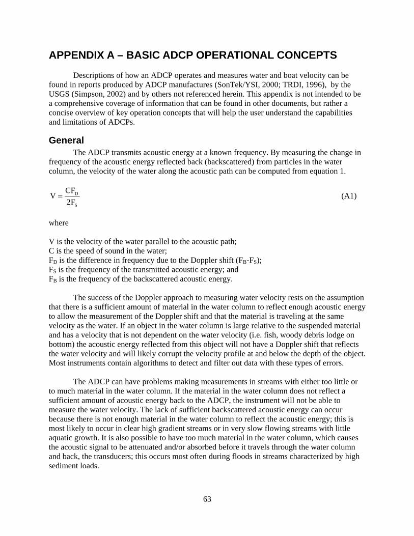
63

APPENDIX A – BASIC ADCP OPERATIONAL CONCEPTS

Descriptions of how an ADCP operates and measures water and boat velocity can be found in reports produced by ADCP manufactures (SonTek/YSI, 2000; TRDI, 1996), by the USGS (Simpson, 2002) and by others not referenced herein. This appendix is not intended to be a comprehensive coverage of information that can be found in other documents, but rather a concise overview of key operation concepts that will help the user understand the capabilities and limitations of ADCPs.

General The ADCP transmits acoustic energy at a known frequency. By measuring the change in

frequency of the acoustic energy reflected back (backscattered) from particles in the water column, the velocity of the water along the acoustic path can be computed from equation 1.

S

D

F2CFV = (A1)

where V is the velocity of the water parallel to the acoustic path; C is the speed of sound in the water; FD is the difference in frequency due to the Doppler shift (FB-FS); FS is the frequency of the transmitted acoustic energy; and FB is the frequency of the backscattered acoustic energy.

The success of the Doppler approach to measuring water velocity rests on the assumption that there is a sufficient amount of material in the water column to reflect enough acoustic energy to allow the measurement of the Doppler shift and that the material is traveling at the same velocity as the water. If an object in the water column is large relative to the suspended material and has a velocity that is not dependent on the water velocity (i.e. fish, woody debris lodge on bottom) the acoustic energy reflected from this object will not have a Doppler shift that reflects the water velocity and will likely corrupt the velocity profile at and below the depth of the object. Most instruments contain algorithms to detect and filter out data with these types of errors.

The ADCP can have problems making measurements in streams with either too little or to much material in the water column. If the material in the water column does not reflect a sufficient amount of acoustic energy back to the ADCP, the instrument will not be able to measure the water velocity. The lack of sufficient backscattered acoustic energy can occur because there is not enough material in the water column to reflect the acoustic energy; this is most likely to occur in clear high gradient streams or in very slow flowing streams with little aquatic growth. It is also possible to have too much material in the water column, which causes the acoustic signal to be attenuated and/or absorbed before it travels through the water column and back, the transducers; this occurs most often during floods in streams characterized by high sediment loads.

64

Figure A-1. Freeway strobe-light system used to measure vehicle speed (from Simpson, 1993)

Measuring Velocity Currently (2007) the two techniques commonly used in an ADCP to measure the Doppler shift can be classified as narrowband or broadband. Each approach has its advantages and disadvantages. A detailed explanation of each technique is beyond the scope of this report and some of the specifics of their implementation into commercial instruments are considered proprietary. However, the basics of the two approaches will be described using an analogy developed by Joel Gast (TRDI, oral commun., 1992) and published by Simpson (2002).

Narrowband Consider a freeway at night with traffic moving at a steady rate of speed. A camera has been placed near the freeway and posts have been installed at set distances within the camera's field of view. A strobe light is actuated and, while the freeway is illuminated by the single-strobe pulse, the camera takes two high-speed photographs. The investigator examines the photographic negatives and lines up the images of the cars on the two photographic negatives and determines the distance traveled by the cars by measuring the apparent shift in position of the reference posts (figure A-1). The speed of the cars can be calculated by multiplying distance between the posts by the lag time between the two photos. If the strobe flashes represent acoustic pulses, the cars represent reflective particles in the water column, and the negatives represent the received reflected signals, this scenario becomes roughly analogous to the workings of a narrowband ADCP system.

The drawback to this approach is that the strobe (pulse length) dissipates very quickly and the two photos must be taken while the same cars are still illuminated by the strobe. This means that time lag between negatives (received signals) are very short and the distance traveled by the cars (reflectors) is very short; therefore, the car speeds cannot be measured precisely. Because of these limitations, velocity measurements made using the narrowband technology are “noisy” (have a relatively high random error). The signal is sampled twice during the reception of the reflected signal. Using an autocorrelation technique, the Doppler shift is then calculated. In the narrowband ADCP, the pulse length depends on the time lag between samples, which is a function of depth cell size. A filter scheme that looks at the whole returned signal is used to resolve ambiguity.

The high random errors of the narrowband system are overcome by averaging. The standard deviation of random noise about a true mean is reduced by the square root of the number of measurements used to computed the mean (Ott, 1988). The narrowband ping is simple

65

and can be processed quickly. Current (2007) narrowband systems can ping at rates up to 20 Hz. Therefore, by pinging fast and averaging the velocity measurement of each ping a narrowband ADCP can measure water velocity with random noise standard deviations of between 12 cm/s and 30 cm/s for 1 second of averaging and between 5 cm/s and 13 cm/s for commonly used 5-second averages.

Broadband Using the same freeway analogy as before, the investigator installs another camera a

distance of 10 or more car lengths (parallel to the freeway) from the first camera. The investigator can now actuate a strobe, take a picture with the first camera, wait a short time, actuate another strobe, and take a picture with the second camera. If the strobes are timed correctly, the cars will travel from the field of view of the first camera into the field of view of the second camera during the time between photos. The investigator synchronizes the positions of the cars on the two negatives and finds that there is a much longer lag time (time between each strobe versus the time between two photos taken during the same strobe) and that the cars traveled a longer distance. This longer distance of travel and lag time allows the investigator to calculate the speed of the cars with much greater precision than with the single-strobe system. However, the distance between the cameras and the time between each strobe must be chosen carefully. If the investigator waits too long between strobes, random movement between the cars (passing, slowing down, speeding up, and so forth) will render the two negatives “unmatchable” (uncorrelated). Transmitting a pair of pulses (strobes) into the water allows for much longer lag times (therefore, more precision) than the narrowband system but there are some “costs” associated with this technique.

One of the most significant costs is self noise. Self noise again can be described using the freeway analogy. Suppose that, because of limitations in photographic technology, the freeway cameras have no shutters. Because the investigator must leave the camera shutters open, both cameras will “see” the traffic illuminated by the two strobes. However, only 50 percent of the “scenery” will be usable to both cameras for correlation purposes. For example, the film in camera one is exposed once during the first strobe. The cars then travel out of the field of view of camera one and into the field of view of camera two. However, the film in camera two already has been exposed by the flash of the first strobe and, thus, any cars photographed have left the field of vision. When the second strobe flashes, the film in both cameras is again exposed (double exposed) and the cars that were first photographed by camera one are now photographed by camera two. Because the film has been double exposed, only 50 percent of the scenery in each exposure contains cars that are common to both cameras. As in the film of the freeway cameras, the reflected wave front from the first pulse-pair is again “exposed” by the incident wave front of the second pulse and, therefore, is subject to the same “double exposure.” The increased noise due to this 50 percent correlation is reduced by data averaging (very narrow pulses can be used, and, therefore, large amounts of data can be collected and averaged). Without a technique called phase coding and a high signal-processing rate, velocity measurements would be less precise (because of self noise) than measurements made by the narrowband ADCP system.

The broadband approach makes use of very narrow (short) pulses. If these pulses were so narrow that 100 of them can be placed into the space occupied by the original long pulses the measurement precision would be increased by the square root of the number of samples (in the

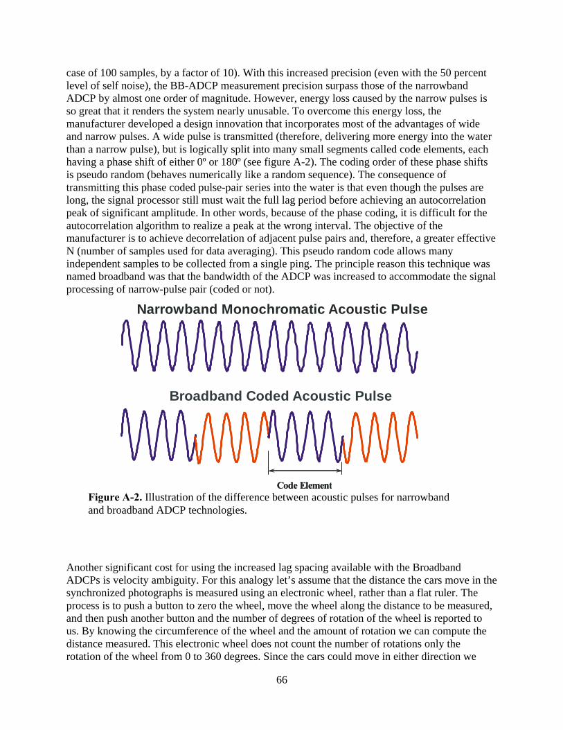
66

case of 100 samples, by a factor of 10). With this increased precision (even with the 50 percent level of self noise), the BB-ADCP measurement precision surpass those of the narrowband ADCP by almost one order of magnitude. However, energy loss caused by the narrow pulses is so great that it renders the system nearly unusable. To overcome this energy loss, the manufacturer developed a design innovation that incorporates most of the advantages of wide and narrow pulses. A wide pulse is transmitted (therefore, delivering more energy into the water than a narrow pulse), but is logically split into many small segments called code elements, each having a phase shift of either 0º or 180º (see figure A-2). The coding order of these phase shifts is pseudo random (behaves numerically like a random sequence). The consequence of transmitting this phase coded pulse-pair series into the water is that even though the pulses are long, the signal processor still must wait the full lag period before achieving an autocorrelation peak of significant amplitude. In other words, because of the phase coding, it is difficult for the autocorrelation algorithm to realize a peak at the wrong interval. The objective of the manufacturer is to achieve decorrelation of adjacent pulse pairs and, therefore, a greater effective N (number of samples used for data averaging). This pseudo random code allows many independent samples to be collected from a single ping. The principle reason this technique was named broadband was that the bandwidth of the ADCP was increased to accommodate the signal processing of narrow-pulse pair (coded or not).

Another significant cost for using the increased lag spacing available with the Broadband ADCPs is velocity ambiguity. For this analogy let’s assume that the distance the cars move in the synchronized photographs is measured using an electronic wheel, rather than a flat ruler. The process is to push a button to zero the wheel, move the wheel along the distance to be measured, and then push another button and the number of degrees of rotation of the wheel is reported to us. By knowing the circumference of the wheel and the amount of rotation we can compute the distance measured. This electronic wheel does not count the number of rotations only the rotation of the wheel from 0 to 360 degrees. Since the cars could move in either direction we

Code Element

Broadband Coded Acoustic Pulse

Code Element

Narrowband Monochromatic Acoustic Pulse

Figure A-2. Illustration of the difference between acoustic pulses for narrowband and broadband ADCP technologies.

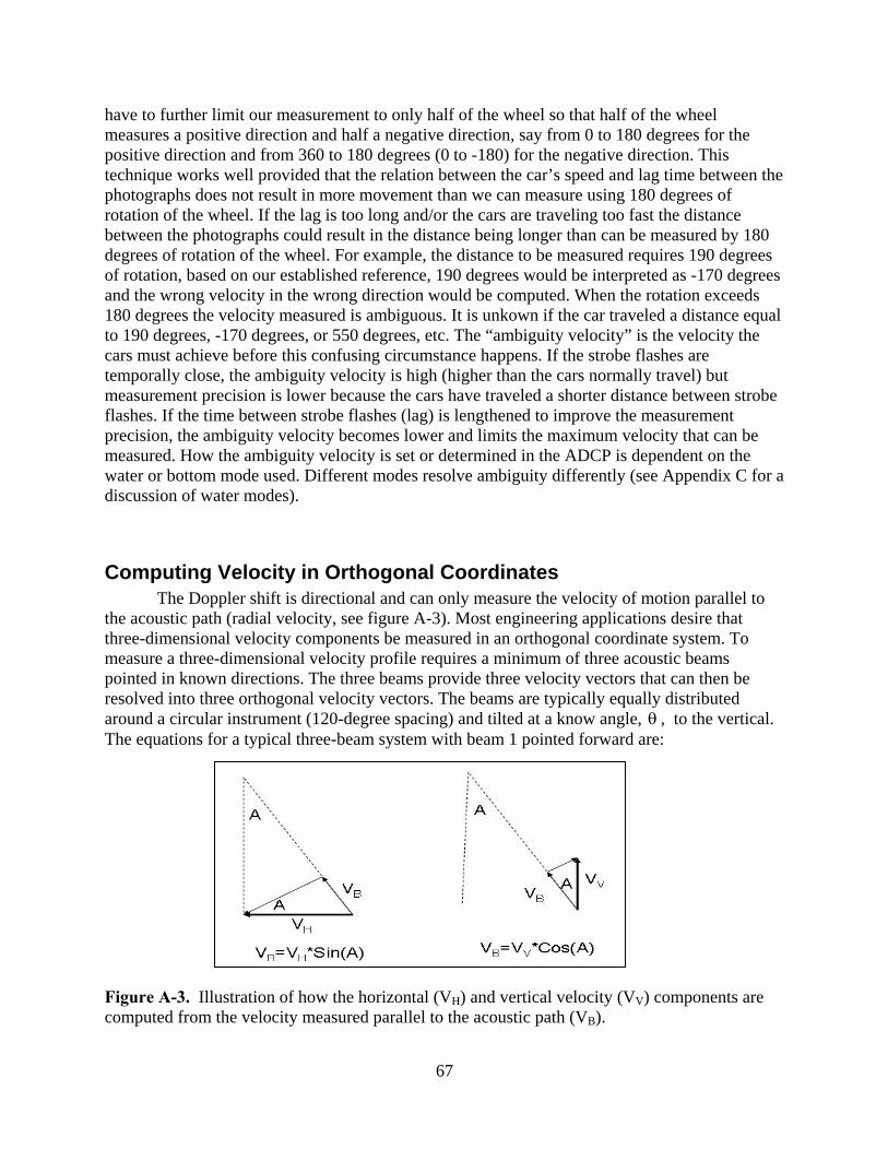
67

have to further limit our measurement to only half of the wheel so that half of the wheel measures a positive direction and half a negative direction, say from 0 to 180 degrees for the positive direction and from 360 to 180 degrees (0 to -180) for the negative direction. This technique works well provided that the relation between the car’s speed and lag time between the photographs does not result in more movement than we can measure using 180 degrees of rotation of the wheel. If the lag is too long and/or the cars are traveling too fast the distance between the photographs could result in the distance being longer than can be measured by 180 degrees of rotation of the wheel. For example, the distance to be measured requires 190 degrees of rotation, based on our established reference, 190 degrees would be interpreted as -170 degrees and the wrong velocity in the wrong direction would be computed. When the rotation exceeds 180 degrees the velocity measured is ambiguous. It is unkown if the car traveled a distance equal to 190 degrees, -170 degrees, or 550 degrees, etc. The “ambiguity velocity” is the velocity the cars must achieve before this confusing circumstance happens. If the strobe flashes are temporally close, the ambiguity velocity is high (higher than the cars normally travel) but measurement precision is lower because the cars have traveled a shorter distance between strobe flashes. If the time between strobe flashes (lag) is lengthened to improve the measurement precision, the ambiguity velocity becomes lower and limits the maximum velocity that can be measured. How the ambiguity velocity is set or determined in the ADCP is dependent on the water or bottom mode used. Different modes resolve ambiguity differently (see Appendix C for a discussion of water modes).

Computing Velocity in Orthogonal Coordinates The Doppler shift is directional and can only measure the velocity of motion parallel to

the acoustic path (radial velocity, see figure A-3). Most engineering applications desire that three-dimensional velocity components be measured in an orthogonal coordinate system. To measure a three-dimensional velocity profile requires a minimum of three acoustic beams pointed in known directions. The three beams provide three velocity vectors that can then be resolved into three orthogonal velocity vectors. The beams are typically equally distributed around a circular instrument (120-degree spacing) and tilted at a know angle, θ , to the vertical. The equations for a typical three-beam system with beam 1 pointed forward are:

Figure A-3. Illustration of how the horizontal (VH) and vertical velocity (VV) components are computed from the velocity measured parallel to the acoustic path (VB).

68

)Sin3/()B2BB(V 132y θ−+= (A2)

)Sin3/()BB(V 23x θ−= (A3) )Cos3/()BBB(V 321z θ++= (A4)

where Vy is the streamwise velocity assuming beam 1 is pointed upstream; Vx is the cross-stream velocity assuming beam 1 is pointed upstream; Vz is the vertical velocity; B1 is the radial velocity measured in beam 1; B2 is the radial velocity measured in beam 2; B3 is the radial velocity measured in beam 3; and θ is the tilt angle of the beams referenced to vertical.

The use of four beams in a Janus configuration is also common in ADCPs. The Janus configuration provides some reduction in errors caused by pitch and roll and random instrument noise for the orthogonal velocity components. The equations for a typical four-beam system with beam 3 pointed forward are:

)2/()( 34 θSinBBVy −= (A5)

)2/()( 21 θSinBBVx −= (A6) )Cos4/()BBBB(V 4321z θ+++= (A7)

where Vy is the streamwise velocity assuming beam 3 is pointed upstream; Vx is the cross-stream velocity assuming beam 3 is pointed upstream; Vz is the vertical velocity; B1 is the radial velocity measured in beam 1; B2 is the radial velocity measured in beam 2; B3 is the radial velocity measured in beam 3; B4 is the radial velocity in beam 4; and θ is the tilt angle of the beams referenced to vertical. The assumption in applying equations A2-A7 is that the flow measured in each beam is the same (homogeneous). If the flow measured by one beam is different than any of the other beams (one beam is measuring in a vortex and the others are in the free stream) the basic assumption of these equations is violated and an incorrect velocity will be computed. Therefore, the velocities measured by an ADCP is less certain in flow conditions with high and rapid spatial variations.

Four-beam systems have a redundant beam that can be used to compute an error velocity. The error velocity is computed as the difference between the vertical velocity computed by opposing beam pairs (3 and 4 versus 1 and 2). Adding the opposing pairs cancels the horizontal velocity leaving only the vertical component.

69

( )θθθ

CosBBBBCos

BBCos

BBV ue 2/)(

22 43214321 −−+=

+−

+= (A8)

where

ueV is the unscaled error velocity.

TRDI scales the error velocity so that the standard deviation for the error velocity is equal to the standard deviation of the horizontal velocity. The equation used to compute the scaled error velocity is:

( )[ ] ( )[ ] )22/()(212/)( 43214321 θθθ SinBBBBTanCosBBBBVerror −−+=−−+= (A9) where errorV is the scaled error velocity computed by TRDI ADCPs.

Measuring a Velocity Profile The ADCP profiling capability is accomplished by time gating (and sampling) the

received acoustic signal at time intervals as the acoustic-beam wave vertically traverses the water column. The transmitted acoustic pulse travels at the speed of sound through the water vertically and is reflected back towards the transducer. Acoustic energy reflected from particles deeper in the water column takes a longer time to arrive back to the transducer than does acoustic energy reflected from particles nearer the transducer. By measuring the two-way travel time from transmission of the energy to when the energy is received, the distance from the transducer from which the energy is reflected can be computed. The ADCP transmits a ping along each acoustic beam and then time gates the reception of the returned echo on each beam into depth cells at specified ranges. Speed and direction are then calculated (using a center-weighted mean of the velocities measured in the depth cell) and assigned to the center of each depth cell (bin) over the measured vertical.

Computing Discharge An ADCP deployed on a moving boat can compute the discharge in real time while traversing the stream from one bank to the other (Simpson and Oltmann, 1993). Unfortunately the ADCP is unable to measure the entire water column. Near the water surface there is an unmeasured zone associated with immersion of the ADCP into the water, the blanking distance below the transducer where data cannot be collected, and additional unmeasured range dependent on the water mode configuration and the bin size . The ADCP also cannot measure all the way to the streambed due to the potential for side-lobe interference. As the ADCP approaches a stream bank the depths will eventually get too shallow for valid data collection. Therefore, the discharge computed by an ADCP is a summation of the measured portion of the cross section and extrapolated discharge estimates for unmeasured portions of the cross section

70

at the top, bottom, and both banks. The computation of the measured, top, and bottom portions of the cross section occur for each ensemble and the discharge for the edges are added to the total.

RightEdgeBottomMeasuredTopLeftEdge QQQQQQ ++++= (A10) where Q is the total discharge;

LeftEdgeQ is the discharge estimated for the unmeasured area near the left bank;

TopQ is the discharge estimated for the top unmeasured area;

MeasuredQ is the discharge measured directly by the ADCP;

BottomQ is the discharge estimated for the bottom unmeasured area; and

RightEdgeQ is the discharge estimated for the unmeasured area near the right bank. The algorithms commonly used to compute discharge in each portion of the cross section are presented below.

Measured Discharge Traditional point-velocity meters (Rantz and others, 1982) compute discharge as the

product of the cross-sectional area and the mean water velocity perpendicular to the cross-sectional area.

VAQ = (A11)

Where

A is the cross-sectional area; and

V is the mean velocity perpendicular to the cross-sectional area.

The ADCP discharge computation algorithm is based on this same principle. Figure A-3 shows the water and boat velocity vectors for a single bin in an ADCP transect. The cross-sectional area of the bin can be computed as the product of the bin size ( dz ) and ensemble width (W ). The bin size is defined by the instrument configuration. The ensemble width is computed as the product of the boat speed and time between ensembles.

dzdtVdzWA b

r== (A12)

Where

71

Figure A-4. Illustration of boat and water velocity vectors for a single bin in an ADCP ensemble.

bVr

is the magnitude of the boat velocity vector;

and

dt is the time between ensembles.

The discharge for the first ensemble is zero because to compute the ensemble width a time for the previous ensemble is needed to compute dt . The mean velocity can be computed as the product of the magnitude of the water velocity,

wVr

and the unit normal vector of the boat

velocity, nr .

nVV wrr

•= (A13)

The equation for discharge in a bin, binQ , becomes

( ) dzdtVnVQ bwbin

rrr•= (A14)

Applying trigonometric relations equation A14 can be written as,

dzdtVVQ bwbin φsinrr

= (A15)

The product of the vector magnitudes and sine of the internal angle is defined as the vector cross product and the equation for binQ can be written in terms of the water and boat velocity vector components.

( ) ( ) dzdtVVVVdzdtVVQ bxwybywxbwbin −=×=rr

(A16)

The measured portion of the discharge can then be computed as,

∑ ∑= =

=Ensembles

j

Bins

ibinMeasured QQ

1 1 (A17)

Top Discharge The discharge in the unmeasured zone at the water surface must be estimated from the

measured data. The length of the unmeasured zone at the water surface is determined by the draft of the instrument deployment, the blank required to avoid the effects of ringing, the water mode configuration, and bin size (see Limitations of Acoustic Profilers for a detailed discussion of ringing). The methods for estimating the top discharge can be applied to the individual velocity components (approach used by SonTek/YSI) or to the cross product from equation A16 (approach used by TRDI). Both approaches are mathematically identical. For simplicity, only the

72

equations utilizing the cross product are shown herein. The user is referred to Huang (2000) for equations based on individual velocity components.

The simplest assumption for estimating the top discharge is to assume the velocity (cross

product) in the topmost valid bin is a good estimate of the mean velocity between that bin and the water surface. This is typically referred to as the constant extrapolation method.

( ) dtzzQEnsembles

j

btb

bwsTop ∑

=

++ −=1

11χ (A18)

where χ is the velocity cross product; and

wsz is the range from the streambed to the water surface; and

tbz is the range from the streambed to the top of the topmost valid bin. This constant extrapolation method is often used where there is an upstream wind or an irregular velocity profile through the measured portion of the water column.

A valid but slightly more complicated approach is to assume that the water velocity profile follows a logarithmic distribution. Simpson and Oltmann (1993) attempted to calculate discharge using several different methods for profile estimation (Logarithmic and general power law), but found that because of “noisiness” of the ADCP-profile data, the resulting least-squares-derived estimates were unrealistic, especially near the upper part of the profile. A method using a one-sixth power law (Chen, 1989) eventually was chosen because of its robust noise rejection capability during most streamflow conditions.

bza=χ (A19)

where a is a coefficient derived from a least squares fit of the equation to the measured data; z is the range from the streambed to the location of the value of χ ; and b is the exponent commonly assumed to be 1/6. The power law estimation scheme is an approximation only and emulates a Manning-like vertical distribution of horizontal water velocities. Different power coefficients can be used to adjust the shape of the curve fit to emulate profiles measured in an estuarine environment or in areas that have bedforms that produce nonstandard hydrologic conditions. Appling equation A19 and integrating to obtain the top discharge estimate yields,

( )∑=

++ −+

=Ensembles

j

btb

bwsTop dtzz

baQ

1

11

1 (A20)

73

Both SonTek and TRDI provide additional options to estimate the top discharge for nonstandard profiles. SonTek/YSI allows the user to select the number of bins used in the top extrapolation method. TRDI restricts the constant method to use of the top bin only and the power law estimate to using all of the available bins, but provides an additional 3-point slope method to fit situations where wind significantly affects the velocity at the water surface. The user is referred to the manufactures documentation for more detail on these methods.

Bottom Discharge ADCPs cannot measure the water velocity near the streambed due to side-lobe

interference (see Limitations of Acoustic Profilers for a detailed discussion of side-lobe interference). Unlike the top discharge estimation problem where we do not know the velocity at the water surface, we know something about the water velocity at the streambed. From fluid mechanics we know that the water velocity must go to zero at the streambed and that a logarithmic velocity profile is a reasonable approximation of the velocity profile in the boundary layer. Therefore, the power law is always used to compute the discharge in the bottom unmeasured portion of the water column.

∑=

+

+=

Ensembles

j

bbbBottom dtz

baQ

1

1

1 (A21)

where

bbz is the range from the streambed to the bottom of the bottom most valid bin. To better apply this method to situations where profile throughout the water column may not follow a logarithmic distribution, such as for bidirectional flow, SonTek/YSI allows the user to select the number of bins near the bottom that are used in the least squares determination of a . TRDI adds an additional method to their software called ‘No-Slip’ which applies equation A21 but restricts the least squares determination of a to bins in the bottom 20 percent of the profile or in the absence of valid bins in the bottom 20 percent, the last valid bin is used to compute a .

Edge Discharge The unmeasured discharge at the edges of the stream are estimated using a ratio

interpolation method presented by Fulford and Sauer (1986), which can be used to estimate a velocity at an unmeasured location between the riverbank and the first or last measured velocity in a cross section (see figure A-4). The equation for the estimate is

m

m

x

x

dV

dV

= (A22)

where

74

x is a location midway between the riverbank and first or last ADCP-measured ensemble or L/2;

xV is the estimated mean velocity at location x ;

mV is the measured mean velocity at the first or last ADCP-measured subsection (see figure A-4);

xd is the depth at location x; and

md is the depth at the first or last ADCP-measured ensemble (see figure A-4). Fulford and Sauer (1986) defined md and mV as depth and velocity, respectively, at the center of the first or last measured subsection and not the near-shore edge of the ensemble, as presented in equation A22. However, because the ADCP ensembles purposely are kept very narrow at the start and finish of each measurement, the differences between the two applications are not significant (Simpson and Oltmann, 1993). With this method, discharge can be estimated by assuming a triangular area at the edge as,

mmm

mmmLedgeEdge VLd

dd

VLdVAQ 3535.05.0

5.02/ =∗== (A23)

where

EdgeQ is the estimated discharge in the unmeasured edge;

edgeA is the area of the unmeasured edge;

2/LV is the velocity midway between the bank and first or last ADCP-measured ensemble; and L is the distance from the last valid ensemble to the edge of water (see figure A-4). Equation A23 can be written in a more general form which utilizes an edge shape coefficient.

mmeEdge dLVCQ = (A24) where

eC is an edge shape coefficient. The edge shape coefficient can be adjusted by the user to reflect unusual edge shapes or roughness but is commonly set to 0.3535 for triangular edges and 0.91 for rectangular edges. The value for L must be measured and entered by the user (see discussion of laser range finders in Other Equipment). It is also recommended that 10 seconds of data be collected in a near

L

dm Vm

L

dm Vm

Figure A-5. Illustration of components used to calculate estimates of discharge in the unmeasured edges of cross sections.

75

stationary position at the beginning and end of each transect to obtain a good measurement for mV and L .

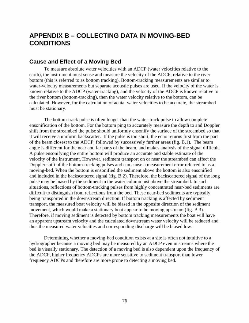
76

APPENDIX B – COLLECTING DATA IN MOVING-BED CONDITIONS

Cause and Effect of a Moving Bed To measure absolute water velocities with an ADCP (water velocities relative to the

earth), the instrument must sense and measure the velocity of the ADCP, relative to the river bottom (this is referred to as bottom tracking). Bottom-tracking measurements are similar to water-velocity measurements but separate acoustic pulses are used. If the velocity of the water is known relative to the ADCP (water-tracking), and the velocity of the ADCP is known relative to the river bottom (bottom-tracking), then the water velocity relative to the bottom, can be calculated. However, for the calculation of acutal water velocities to be accurate, the streambed must be stationary.

The bottom-track pulse is often longer than the water-track pulse to allow complete ensonification of the bottom. For the bottom ping to accurately measure the depth to and Doppler shift from the streambed the pulse should uniformly ensonify the surface of the streambed so that it will receive a uniform backscatter. If the pulse is too short, the echo returns first from the part of the beam closest to the ADCP, followed by successively further areas (fig. B.1). The beam angle is different for the near and far parts of the beam, and makes analysis of the signal difficult. A pulse ensonifying the entire bottom will produce an accurate and stable estimate of the velocity of the instrument. However, sediment transport on or near the streambed can affect the Doppler shift of the bottom-tracking pulses and can cause a measurement error referred to as a moving-bed. When the bottom is ensonified the sediment above the bottom is also ensonified and included in the backscattered signal (fig. B.2). Therefore, the backscattered signal of the long pulse may be biased by the sediment in the water column just above the streambed. In such situations, reflections of bottom-tracking pulses from highly concentrated near-bed sediments are difficult to distinguish from reflections from the bed. These near-bed sediments are typically being transported in the downstream direction. If bottom tracking is affected by sediment transport, the measured boat velocity will be biased in the opposite direction of the sediment movement, which would make a stationary boat appear to be moving upstream (fig. B.3). Therefore, if moving sediment is detected by bottom tracking measurements the boat will have an apparent upstream velocity and the calculated downstream water velocity will be reduced and thus the measured water velocities and corresponding discharge will be biased low.

Determining whether a moving-bed condition exists at a site is often not intuitive to a hydrographer because a moving bed may be measured by an ADCP even in streams where the bed is visually stationary. The detection of a moving bed is also dependent upon the frequency of the ADCP, higher frequency ADCPs are more sensitive to sediment transport than lower frequency ADCPs and therefore are more prone to detecting a moving bed.

77

Figure B.1 An example of short and long bottom track pulses (from Simpson, 2002)

Figure B.2 An example of the potential for water bias (moving bed) for short and long bottom track pulses

Long Pulse

Small area illuminated Large area illuminated

Short pulse

near bottomsediment

suspendedsediment

Bottom

Long backscatteredpulse width

Short backscatteredpulse width

Long Pulse

Small area illuminated Large area illuminated

Short pulse

near bottomsediment

suspendedsediment

Bottom

Long backscatteredpulse width

Short backscatteredpulse width

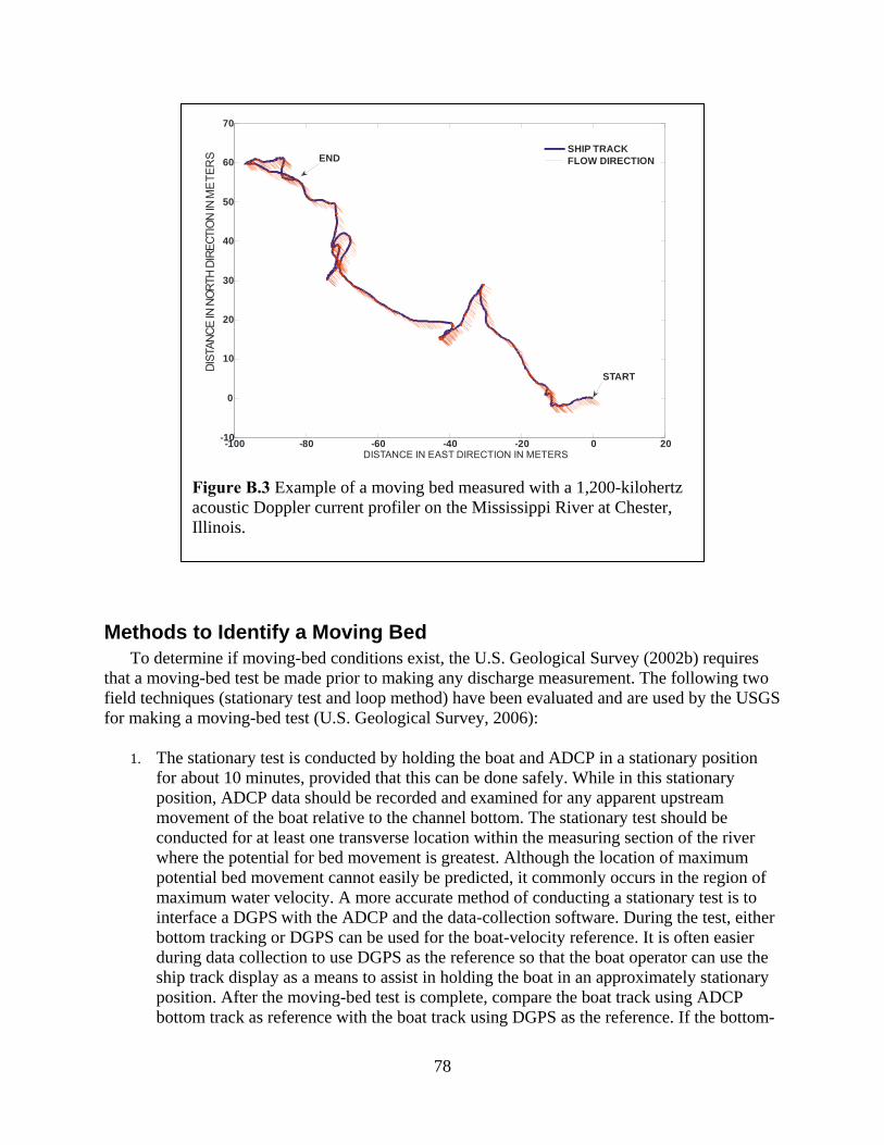
78

Methods to Identify a Moving Bed

To determine if moving-bed conditions exist, the U.S. Geological Survey (2002b) requires that a moving-bed test be made prior to making any discharge measurement. The following two field techniques (stationary test and loop method) have been evaluated and are used by the USGS for making a moving-bed test (U.S. Geological Survey, 2006):

1. The stationary test is conducted by holding the boat and ADCP in a stationary position for about 10 minutes, provided that this can be done safely. While in this stationary position, ADCP data should be recorded and examined for any apparent upstream movement of the boat relative to the channel bottom. The stationary test should be conducted for at least one transverse location within the measuring section of the river where the potential for bed movement is greatest. Although the location of maximum potential bed movement cannot easily be predicted, it commonly occurs in the region of maximum water velocity. A more accurate method of conducting a stationary test is to interface a DGPS with the ADCP and the data-collection software. During the test, either bottom tracking or DGPS can be used for the boat-velocity reference. It is often easier during data collection to use DGPS as the reference so that the boat operator can use the ship track display as a means to assist in holding the boat in an approximately stationary position. After the moving-bed test is complete, compare the boat track using ADCP bottom track as reference with the boat track using DGPS as the reference. If the bottom-

-100 -80 -60 -40 -20 0 20-10

0

10

20

30

40

50

60

70

DISTANCE IN EAST DIRECTION IN METERS

DIST

ANCE

INNO

RTH

DIRE

CTIO

NIN

SHIP TRACKFLOW DIRECTION

START

END

ME

TER

S

Figure B.3 Example of a moving bed measured with a 1,200-kilohertz acoustic Doppler current profiler on the Mississippi River at Chester, Illinois.

79

track boat velocity data indicate apparent upstream movement that the DGPS data do not indicate, a moving bed is present.

The moving-bed velocity (Vmb) measured during the stationary test is determined by dividing the apparent distance the ADCP moved in the upstream direction by the duration of the test. If the moving-bed velocity exceeds 2 percent of the mean water velocity (Vw) for the discharge measurement (Vmb/Vw >0.02) a DGPS should be used to determine boat velocity. If a DGPS is not available or site conditions do not permit its use other approved water bias correction methods (which will be discussed later in Appendix B.) should be applied. However, if the moving-bed test was made using a tethered boat, a manned boat that was anchored in the stream, or if the boat operator was able to keep the boat accurately on station throughout the moving-bed test, DGPS or water bias correction methods should be used when the moving-bed velocity exceeds 1 percent of the mean velocity for the discharge measurement (Vmb/Vw >0.01).

2. The loop method is based on the fact that as an ADCP is moved across the stream, a

moving bed will cause the bottom track-based ship track to be distorted in the upstream direction. Therefore, if an ADCP makes a two-way crossing (loop) of a stream with a moving bed and returns to the exact starting position, the bottom track-based ship track will show that the ADCP returned to a position upstream from the original starting position. When appropriate, using the loop method as a moving-bed test has the advantage of measuring bed conditions throughout the portion of the cross section that can be directly measured with the ADCP. The loop method, therefore, results in a more representative moving-bed test than a single-location stationary moving-bed test. However, it is critical the bottom track be maintained throughout the entire test and that the internal compass in properly calibrated.

The mean moving-bed velocity can be estimated from the distance the ADCP appeared to have moved upstream from the starting position (loop-closure error) and the time required to complete the loop.

TD

V upmb = , (1)

where Vmb is the mean velocity of the moving bed;

upD is the loop-closure error (distance made good, straight-line distance from starting point to ending point); and

T is the measurement time required to complete the loop. These data are readily available from most commercial software used to measure discharge with ADCPs.

80

If the mean moving-bed velocity exceeds 1.2 cm/s and is greater than 1 percent of the mean water velocity (Vw) for the discharge measurement (Vmb/Vw >0.01) a DGPS should be used to determine boat velocity or the loop correction method for correcting discharge should be applied (a detailed discussion of the loop correction method will be discussed later in Appendix E.).

Methods to Account for Moving-Bed Effects The integration of a DGPS to measure the velocity of the ADCP has been shown to

alleviate the systematic errors associated with a moving bed (Mueller, 2002) and is the most accurate way to measure discharge in moving-bed conditions. However, if a DGPS is not available or site conditions do not permit its use, methods have been established to correct discharge measurements biased by a moving bed. The use of DGPS and the application of various discharge correction methods are discussed in the following sections.

Using GPS with ADCPs Using GPS with ADCPs eliminates the effect of a moving-bed on the velocity measurements but introduces several sources of potential error. Understanding how GPS operates and how it is used with ADCPs is important in collecting high quality ADCP measurements when using GPS as the boat velocity reference.

The computation of water velocity from an ADCP mounted onto a moving boat is a vector-algebra problem. The ADCP measures the water velocity relative to the moving boat (relative water velocity), so the velocity of the boat must be accounted for to obtain the true water velocity (WV) (fig. B.4). The true water velocity is computed by subtracting the bottom-tracking velocity (BT) vector from the water-tracking velocity (WT) vector. When bottom tracking is used, the direction of the boat velocity vector ( θBT ) and water-tracking velocity vector ( θWT ) are referenced to the instrument. The ADCP has an internal fluxgate compass to measure the orientation of the instrument ( θInst ) relative to the local ambient magnetic field (magnetic north). The water-tracking ping and the bottom-tracking ping occur separately but both occur within a fraction of a second; a single reading of the compass is used to determine the orientation of the instrument for both pings. The water-velocity vector can be easily referenced to magnetic north by rotating the vector based on the measured θInst . The magnitude of the water velocity is unaffected by any errors in the measurement of θInst when the bottom-tracking ping is used as the boat reference. The basic equation presented in Simpson and Oltmann (1993) for computing measured discharge (exclusive of unmeasured areas) by use of an ADCP mounted onto a moving boat is

dtdzsinVVQ b

T

0

D

0 f θ= ∫ ∫rr

where Q is the total discharge; T is the total time for which data were collected;

81

D is the total depth;

fVr

is the mean water-velocity vector;

bVr

is the mean boat-velocity vector; θ is the angle between the water-velocity vector and the boat velocity vector (fig. E.5); dz is the vertical differential depth; and dt is differential time.

Figure B.4. Vectors used for computing the water-velocity vector (from Mueller, 2002). To compute the discharge, only the angle between the water-velocity and the boat velocity vectors is needed. When bottom tracking is used, the direction of the relative water-velocity (WT) vector and the boat velocity (BT) vector are referenced to the instrument (fig. B.5a). When DGPS is used to determine the boat-velocity vector, this vector is referenced to true north by use of the DGPS coordinates (fig. B.5b). The orientation of the instrument relative to true north must be determined to put the boat-velocity vector and the relative water-velocity vector in the same coordinate system and allow the computation of the water-velocity vector (WV) and θ . The discharge is affected by errors in measuring Instθ and in the determination of the magnetic variation ( Magθ ) when DGPS is used as the boat reference. The errors associated with measuring

Instθ can cause errors in the measured discharge that are proportional to the speed of the boat. Proper setup and calibration of the ADCP’s internal compass, determination of the local magnetic variation, and a slow boat speed are critical to discharge measurements made using DGPS as the boat-velocity reference.

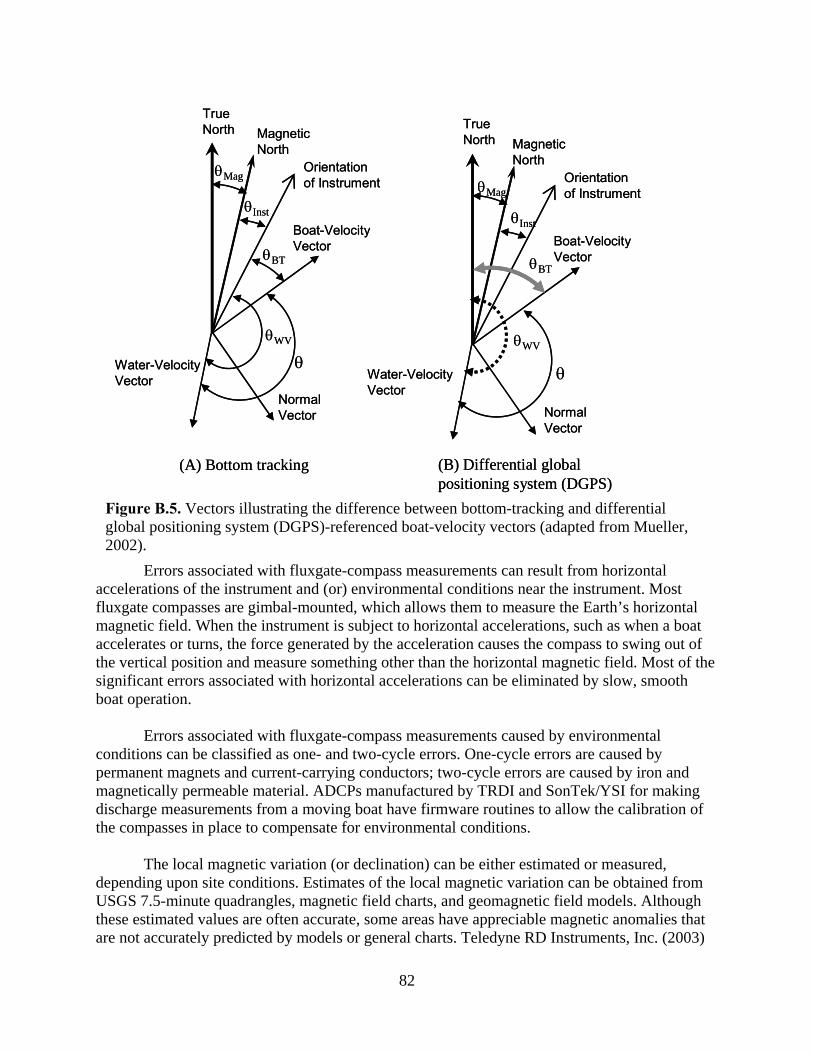
82

Errors associated with fluxgate-compass measurements can result from horizontal accelerations of the instrument and (or) environmental conditions near the instrument. Most fluxgate compasses are gimbal-mounted, which allows them to measure the Earth’s horizontal magnetic field. When the instrument is subject to horizontal accelerations, such as when a boat accelerates or turns, the force generated by the acceleration causes the compass to swing out of the vertical position and measure something other than the horizontal magnetic field. Most of the significant errors associated with horizontal accelerations can be eliminated by slow, smooth boat operation.

Errors associated with fluxgate-compass measurements caused by environmental conditions can be classified as one- and two-cycle errors. One-cycle errors are caused by permanent magnets and current-carrying conductors; two-cycle errors are caused by iron and magnetically permeable material. ADCPs manufactured by TRDI and SonTek/YSI for making discharge measurements from a moving boat have firmware routines to allow the calibration of the compasses in place to compensate for environmental conditions.

The local magnetic variation (or declination) can be either estimated or measured, depending upon site conditions. Estimates of the local magnetic variation can be obtained from USGS 7.5-minute quadrangles, magnetic field charts, and geomagnetic field models. Although these estimated values are often accurate, some areas have appreciable magnetic anomalies that are not accurately predicted by models or general charts. Teledyne RD Instruments, Inc. (2003)

θ

NormalVector

TrueNorth Magnetic

NorthOrientationof Instrument

Boat-VelocityVector

Water-VelocityVector

nstΙθ

Magθ

BTθ

WVθ

θ

NormalVector

TrueNorth Magnetic


Boat-VelocityVector


nstΙθ

Magθ

BTθ

WVθ

(A) Bottom tracking (B) Differential global positioning system (DGPS)

θ

NormalVector

TrueNorth Magnetic


Boat-VelocityVector


nstΙθ

Magθ

BTθ

WVθ

θ

NormalVector

TrueNorth Magnetic


Boat-VelocityVector


nstΙθ

Magθ

BTθ

WVθ

(A) Bottom tracking (B) Differential global positioning system (DGPS)

Figure B.5. Vectors illustrating the difference between bottom-tracking and differential global positioning system (DGPS)-referenced boat-velocity vectors (adapted from Mueller, 2002).

83

documents a procedure for measuring the magnetic variation on site by use of an ADCP and a DGPS. This same procedure can be used with RiverSurveyor instruments and RiverSurveyor software from SonTek/YSI. The limitation of this procedure is that there can be no moving-bottom conditions because both the bottom tracking and DGPS are used in the computations.

The DGPS receivers used for ADCP discharge measurements made from a moving boat should be accurate within less than a meter. Although the differential correction accounts for errors induced by the ionosphere, atmosphere and selective availability, the user must be aware of and take action to minimize uncorrectable errors, which can be caused by the user, the satellite configuration, or the characteristics of the site. It is important to locate the DGPS antenna as near to the center of the ADCP as possible so that the direction of travel is the same for both the antenna and the ADCP during all boat maneuvers. The antenna should be located above the boat cabin or other accessories on the boat to eliminate multi-path errors. Multi-path errors are positional errors that arise when satellite signals bounce around before getting to the receiver, rather than taking a direct path. The result is a barrage of signals arriving at the receiver: first the direct one, then a series of delayed reflected ones. This creates a noisy signal and if the bounced signals are strong enough they can confuse the receiver and cause erroneous positional measurements. Sophisticated receivers use a variety of signal processing techniques to make sure that they only consider the earliest arriving signals (which are the direct ones) and although these techniques reduce multi-path errors, they do not completely eliminate the problem.

Occasionally, the configuration of the satellites does not allow an accurate determination of the horizontal position. This can be monitored using the horizontal dilution of precision (HDOP). If the HDOP parameter is greater than 2 or the HDOP changes by more than 1 during a transect, the quality of the DGPS positions is suspect. Local site characteristics such as canyon walls, bluffs, tall buildings, and tree cover can result in poor DGPS positions because of multi-path errors and loss of satellite visibility. Poor satellite visibility often results in numerous changes in the number and configuration of satellites used to determine a position. Numerous changes in satellites are another indication that the quality of the DGPS positions may be poor. In addition to horizontal-position coordinates, the DGPS also computes elevation. This elevation is 2 to 4 times less accurate than the horizontal position (Mueller, 2002). The elevation of the boat should be reasonably constant. Changes greater than 3.5 meters (m) in the DGPS-determined elevation indicate that the quality of the DGPS positions may be poor (Teledyne RD Instruments, Inc., WinRiver 10.06 Help File, written commun., 2006).

To determine ADCP movement when bottom tracking is biased or not working,

manufacturer software historically has utilized only the differentially corrected GGA data string broadcast by the GPS, which includes time, positional data (latitude, longitude, elevation) and information about the satellite constellation used to reach the position solution. Positional accuracy is extremely important when using GGA data string from the GPS to measure the movement of the ADCP because the velocity of the instrument is determined by computing the distance traveled between successive GPS position solutions and dividing that distance by the time between the solutions. Hence, positional accuracy is vitally important to achieve an accurate measure of ADCP movement using the GGA data string and therefore a differential correction signal is required.

84

While GPS is most often used to determine positions, many GPS receivers can also be used to measure velocity relative to ground with an assessment of the Doppler shift in the satellite carrier phase frequencies. The method uses the actual signal frequency, not a phase angle to determine the Doppler shift. So there cannot be any ambiguity in the computed velocities. As for the position determination, the velocity measurement requires the use of at least 4 satellites. The quality of the solution is also influenced by the number of satellites and the shape of the constellation (HDOP) during the observation. The great advantage of this alternative is that it is minimally impacted by multi-path and satellite changes due to the short sampling time required. In addition, multi-path and ionospheric/atmospheric distortions do not affect the precision of the measurement. As a result, the Doppler measurement of velocity can be produced without the need for any differential correction. Emerging research by Environment Canada and the USGS using the VTG data string from the GPS (which provides the Doppler measurement of velocity relative to the ground and data on direction and speed) has shown the potential to provide better measurements of ADCP movement than the GGA data string without the need for differential correction.

Alternatives to Using GPS The integration of a differentially corrected Global Positioning System (DGPS), to

measure the velocity of the ADCP, has been shown to alleviate the systematic errors associated with a moving bottom (Mueller, 2002). DGPS systems, however, will not work in all conditions. For example, a DGPS will have trouble providing consistently accurate positions and velocities on waterways with dense tree canopy along the banks, in deep valleys or canyons, and near bridges owing to multi-path and satellite signal reception problems. Alternative methods of correcting for the systematic moving-bottom error have been developed for situations where integrating DGPS with an ADCP is not possible.

Subsection Method The first GPS alternative requires the hydrographer to make multiple stationary moving-

bed tests across the stream (see figure B.6), subsection the measurement into areas corresponding to each moving-bed test, and apply a moving-bed correction factor to the different portions of the discharge measurement. The field and processing procedures for the subsection method are summarized below.

Field Procedures: 1. Make 4 or 5 stationary moving-bed tests and note the location of each test by measuring the

distance from shore. Be sure to record these tests and the locations. 2. Make a normal ADCP discharge measurement.

Processing Procedures:

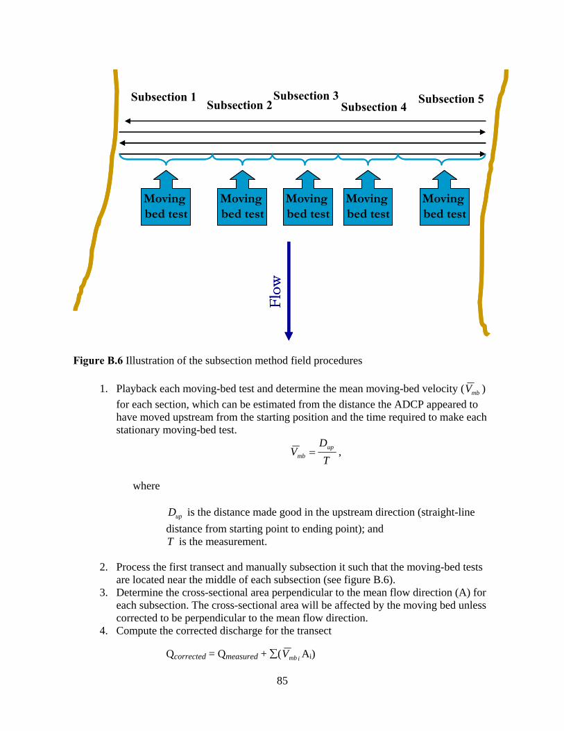
85

1. Playback each moving-bed test and determine the mean moving-bed velocity ( mbV ) for each section, which can be estimated from the distance the ADCP appeared to have moved upstream from the starting position and the time required to make each stationary moving-bed test.

TD

V upmb = ,

where

upD is the distance made good in the upstream direction (straight-line distance from starting point to ending point); and T is the measurement.

2. Process the first transect and manually subsection it such that the moving-bed tests

are located near the middle of each subsection (see figure B.6). 3. Determine the cross-sectional area perpendicular to the mean flow direction (A) for

each subsection. The cross-sectional area will be affected by the moving bed unless corrected to be perpendicular to the mean flow direction.

4. Compute the corrected discharge for the transect

Qcorrected = Qmeasured + ∑( imbV Ai)

Moving bed test

Moving bed test

Moving bed test

Moving bed test

Moving bed test

Flow

Moving bed test

Moving bed test

Moving bed test

Moving bed test

Moving bed test

Flow

Flow

Subsection 1 Subsection 2

Subsection 3Subsection 4

Subsection 5

Figure B.6 Illustration of the subsection method field procedures

86

where imbV is the moving-bed velocity in the subsection i; Ai is the cross-sectional area perpendicular to flow in subsection i; and Qmeasured is the total unadjusted (biased) discharge for the transect.

5. Follow steps 2 through 4 for each transect collected as part of the discharge measurement. The mean of the Qcorrected for all transects is the corrected discharge for the measurement.

The advantage to using the subsection method is that a DGPS is not required; however the disadvantages are 1) method is not currently supported in software, 2) multiple moving-bed tests are required, 3) there is no correction for ADCP movement during the moving-bed tests, 4) the procedure is time consuming, 5) an accurate cross-sectional area projected perpendicular to the mean flow direction is required, and 6) while the discharges are corrected, measured velocities are still biased low.

Section by Section Method The second GPS alternative is referred to as the section by section method and utilizes

the ADCP to measure discharge in manner similar to a standard cup-meter measurement. The hydrographer collects 20-25 velocity profiles with the ADCP at selected locations across the stream. A stationary water-velocity profile is collected by holding the ADCP in a specific location for a specified time and then averaging the data to obtain a mean velocity profile or a depth-integrated mean velocity at that location. The section-by-section method is not biased by moving-bed conditions because the ADCP is held stationary for each measurement and bottom tracking is not referenced; therefore, the velocity measured by the ADCP is only the water velocity. Is it very important for the boat reference to be set to “none” in software when making a section by section measurement in moving-bed conditions or the measured velocity will still be biased by the moving bed.

SonTek/YSI, Inc. has developed software that supports section-by-section discharge measurements collected using their RiverSurveyor ADCPs. The software collects the velocity and depth data from the ADCP and computes the discharge using the mid-section method. The width for each measurement section is computed as half the distance from the current section to the previous section, plus half the distance from the current section to the next section. This width is then multiplied by the depth measured during the velocity measurement to compute an area for each section. Discharge for each of the sections is then computed by multiplying the mean water velocity by the cross-sectional area and then the incremental discharges are summed to determine the total discharge.

Teledyne RD Instruments ADCP software (WinRiver 10.06) currently (2007) does not support (although development is ongoing) section by section measurements; therefore discharge computations must be done manually. The correct way to average the velocity data for each section is to compute the mean velocity profile and then compute the mean velocity from the mean profile. This method computes the mean velocity in each bin of the profile and then computes the mean velocity of the profile from the mean velocity in each bin. The mean velocity

87

for each profile should be determined by computing the mean east velocity component and the mean north velocity component and then computing the magnitude of the velocity by taking the square root of the sum of the squares of the components.

22

⎟⎟⎠

⎞⎜⎜⎝

⎛+⎟

⎟⎠

⎞⎜⎜⎝

⎛= ∑∑

nV

nV

V ne

where

V is the mean water speed;

eV is the east component of the water velocity in each bin;

nV is the north component of the water velocity in each bin; and n is the number of bins with valid water velocity components.

The WinRiver 10.06 software does not compute the mean water velocity in this manner directly but it can easily be computed from the “Velocity Tabular View” with reference set to “none” and all of the ensembles for the section averaged together. The discharge is then computed using the mid-section method previously described.

The advantages to using the section-by-section method is that 1) a DGPS is not required, 2) correct velocities are measured, 3) discharge measurements procedures are familiar to hydrographers, 4) software is available for the RiverSurveyor. The disadvantages are 1) positions must be manually measured, 2) angled flow can introduce errors in the velocity measurement and must be handled carefully, 3) appropriate sampling times are required for each measurement, 4) the ADCP must be kept stationary because there is no correction of ADCP movement, and 5) the entire cross section is not measured.

Azimuth Method The third GPS alternative is referred to as the azimuth method. The azimuth method is

based on the fact that as an ADCP moves across the stream, a moving bed will cause the bottom-track based ship track to be distorted in the upstream direction. If the azimuth between the starting and ending point of an ADCP transect is known, and the compass on the ADCP has been properly calibrated, the difference in azimuth of the course of the transect from that manually measured and that determined by the ADCP is a measure of the moving-bed velocity and can be used to compute a correction factor for the transect (see figure B.7). The field and processing procedures for the azimuth method are summarized below.

88

Field Procedures:

1. Establish starting and ending points and mark with buoys or other markers. It is important that you start and stop the measurement as closely as possible to these points (within 1 foot, if possible).

2. Use a handheld compass to measure the azimuth from one buoy or marker to the other and record this number.

3. Calibrate the compass on the ADCP using the internal calibration routines. 4. Collect data as normal, but make special care to start and stop the transects at the buoys

or markers.

Processing Procedures:

1. Process the measurement as you normally would. 2. For each transect, note the Distance Made Good, the Course Made Good, Q/A, and the

total time for the transect. 3. Determine the difference between the measured azimuth and the course made good and

call this difference, C. This angle should be in the upstream direction (see figure E.7).

refmg CCC −= where

C = angle between the manually measured and ADCP measured course; Cmg = azimuth of course made good measured by ADCP; and Cref = azimuth of course made good measured manually with a compass.

4. The moving-bed correction factor for each transect can be computed as:

TCD

V MGmb

)sin(×=

Flow

Azimuth of course made good effected by moving bed (Cmg)

Azimuth of true course made good (Cref)

C

DMG

Distance moved upstream

Flow

Azimuth of course made good effected by moving bed (Cmg)

Azimuth of true course made good (Cref)

C

DMG

Distance moved upstream

Figure B.7 Illustration of the azimuth method.

89

where

Vmb is the moving-bed velocity;

DMG is the distance made good; and T is the total measurement time for the transect.

5. Determine the cross-sectional area perpendicular to the mean flow direction (A) for the transect. The cross-sectional area will be affected by the moving bed unless corrected to be perpendicular to the mean flow direction.

6. Compute the corrected discharge for the transect

Qcorrected = Qmeasured + ( mbV A) where mbV is the moving-bed velocity for the transect; A is the cross-sectional area perpendicular to flow for the transect; and Qmeasured is the total unadjusted (biased) discharge for the transect.

7. Follow steps 2 through 6 for each transect collected as part of the discharge measurement. The mean of the Qcorrected for all transects is the corrected discharge for the measurement.

The advantages to using the subsection method are that a DGPS is not required and computations are simple. The disadvantages are 1) start and stop markers must be established, 2) the accuracy is dependent upon the measured azimuth and actual start and stop locations, 3) a compass calibration is required, 4) an accurate cross-sectional area projected perpendicular to the mean flow direction is required, 5) measured velocities are still biased low, 6) bottom tracking must be maintained, and 7) field applications have shown variable accuracy due to errors in azimuth measurements.

Loop Method The loop method is based on the fact that as an ADCP moves across the stream, a moving

bed will cause the bottom-track based ship track to be distorted in the upstream direction. Therefore, if an ADCP makes a two-way crossing of a stream (loop) with a moving bed and returns to the exact starting position, the bottom-track based ship track will show that the ADCP will have returned to a position upstream of the original starting position (figure B.8). Because the ADCP appears to have moved upstream, the water velocity measured by the ADCP will be biased low and consequently the discharge will be biased low. If the moving-bed velocity can be determined, the discharge missing from the measurement caused by the moving bed could be computed and added to the measured discharge to yield a corrected discharge.

mbTMTC QQQ += (1)

where

TCQ is the discharge corrected for the moving-bed bias;

90

TMQ is the measured discharge; and

mbQ is the discharge missed caused by the moving bed. A detailed analysis of the application of the loop method was conducted by the USGS (Mueller and Wagner, 2006).

Careful field procedures are absolutely critical to the successful application of the loop method. Failure to accurately return the instrument to the starting point, an uncalibrated or improperly calibrated compass, or loss of bottom track during the loop will result in unpredictable errors that render this technique unusable. Current research (which is limited by the amount of available field data) indicates that site-specific characteristics and data collection techniques such as the shape of the measurement section, distribution of the moving-bed velocity, time spent at the banks, boat speed, and uniformity of the boat speed can affect the discharge correction by 10 percent or greater. When applied properly, however this technique should consistently yield total corrected discharges that are within 5 percent of the actual discharge.

Field Procedures: 1. Calibrate the ADCP/ADP compass using internal calibration routines. A compass

-100 -50 0 50 100 150

-250

-200

-150

-100

-50

0

50

Distance East in m

Dis

tanc

e N

orth

in m



Dis

tanc

e no

rth in

met

ers

-100 -50 0 50 100 150

-250

-200

-150

-100

-50

0

50

Distance East in m

Dis

tanc

e N

orth

in m



Dis

tanc

e no

rth in

met

ers

Figure B.8. Example of the distorted ship track in a loop caused by a moving bed.

91

calibration accuracy of better than 1 degree is desired. Calibrations with errors greater than 1 degree should be repeated. If after several attempts a calibration of less than 1 degree cannot be obtained appropriate field notes should be recorded to document the problem. Compass errors greater than 1 degree result in increased errors in the loop method correction.

2. Establish a marked starting point where the ADCP/ADP can be returned to the exact location. This point is not required to be as near to a bank as the end of a regular transect. For example, with a tethered boat it can be hard to control the boat at the edge because of conditions such as slack water, eddies, or vegetation, therefore establishing a point farther out in the flow could make navigating the boat back to the starting point more practical. Use of a buoy or other fixed object is recommended.

3. Make a steady pass back and forth across the stream as a normal discharge measurement, but do not stop recording at the far bank. At the starting point make sure the boat is ready to begin the transect before beginning to record. A uniform boat speed is important. Do not spend extra time at the edges. Plan the loop so that a smooth change in boat direction can be achieved near the far bank. Too much time near the banks will result in a low bias.

4. Maintain the proper boat speed. The recommended maximum boat speed should be the lesser of a boat speed that requires no less than 3 minutes to complete the loop or a boat speed that is less than 1.5 times the mean water speed.

5. Return to the starting point. Return position accuracy is very important.

Processing Procedures for Use as a Moving-Bed Test: 1. Process the loop file to the end. Record the Distance Made Good (DMG) and the time

required to complete the loop. Note: The DMG in a moving-bed condition should be in the upstream direction (see fig. B.8). If the primary direction of the DMG is in a direction other than upstream, this distance may be the result of compass or bottom-track errors and no moving bed will be assumed.

2. Compute the mean moving-bed velocity.

TD

V upmb = ,

where

mbV is the mean velocity of the moving bed;

upD is the Distance Made Good (DMG); and T is the measurement time required to complete the loop.

3. Compute the ratio of the mean moving-bed velocity to the mean water velocity. 4. Determine if the ratio exceeds the recommended criteria. In order to minimize the potential

error in the measured moving-bed bias when using the loop method as a moving-bed test, the hydrographer should utilize the following thresholds in determining and applying a correction for an apparent moving streambed.

92

• When using the loop method, a measured mean moving-bed velocity of at least 1.2 cm/s indicates the presence of a moving-bed.

• If the measured moving-bed velocity exceeds 1.2 cm/s, the ratio of the mean moving-bed velocity and mean water velocity should be computed.

• If this ratio is greater than 0.01, the apparent bed movement will cause at least a 1 percent negative bias in the computed discharge and a DGPS or method that accounts for or corrects for a moving bed should be used.

Processing Procedures for Correcting Biased Discharge: There are two methods described by Mueller and Wagner (2006) by which the loop

method can be used to correct discharge biased by a moving bed, the mean correction method and distributed correction method. Mean Correction Method

A simple method for computing the discharge missed caused by the moving bed is to compute the mean moving-bed velocity and multiply it by the cross-sectional area (measured perpendicular to the flow).

AVQ mbmb = (2)

where

mbV is the mean velocity of the moving bed; and A is the cross-sectional area perpendicular to the mean flow direction.

The mean moving-bed velocity can be computed from the distance the ADCP appeared to have moved upstream from the starting position (loop-closure error) and the time required to complete the loop.

TD

V upmb = (3)

where

upD is the loop-closure error (distance made good, straight-line distance from starting point to ending point); and T is the measurement time required to complete the loop.

These data are readily available from most commercial software used to measure discharge with ADCPs.

It is important that the cross-sectional area is computed perpendicular to the mean flow direction. If the cross-sectional area is computed parallel to the ship track measured by the ADCP, then the cross-sectional area will be computed based on a ship track that is distorted in the upstream direction by the moving bed. The distortion of the ship track by a moving bed will result in a cross-sectional area that is too large. The mean correction method is simple to apply

93

but does not account for the cross-section shape and spatial correlation of the sediment transport with the spatial distribution of the discharge in the cross section. Therefore, streams with high spatial variability in sediment transport and discharge distributions may not be properly represented by using a single mean moving-bed velocity to correct the measured discharge. Distributed Correction Method

The actual moving-bed velocity at any point in the stream is unknown, but it is reasonable to assume that the moving-bed velocity is proportional to the near-bed water velocity (Callede et al. 2000). The distributed correction method uses a 1/6th power curve to provide a consistent estimate of the near-bed velocity at any point in the cross section. To determine the distributed loop method correction, the measured mean moving-bed velocity from the loop is distributed to each ADCP profile by a ratio of near-bed velocity for each profile and the mean near-bed velocity for the cross section. The distributed moving-bed velocities are then applied to the water and boat velocities for all bins in each of the corresponding profiles in the measured portion of the cross section to determine the corrected measured discharge. The total discharge measured by an ADCP consists of a measured portion and estimates of discharge in the unmeasured top, bottom, left, and right edges. Therefore, the final corrected measured discharge is computed using the ratio of the corrected and uncorrected measured portion of the discharge to correct the sum of the measured and top and bottom estimated discharges. It is assumed that water velocities near the bank will be sufficiently low as to not cause a moving bed and therefore, no correction is applied to the left and right edge discharges.

Distribution of the mean moving-bed velocity based on near-bed velocities requires a consistent method of determining near-bed velocities at each measured vertical. Due to side-lobe interference the lower 6-10 percent, approximately, of each velocity profile is unmeasured. In addition, bad velocity measurements are common in the lower portions of the profile. Therefore, simply using the last valid velocity in each measured velocity profile would result in near-bed velocities at various distances from the streambed. The 1/6th power law has been shown to be consistent with a logarithmic velocity profile and is commonly used to estimate the unmeasured top and bottom discharges for ADCP measurements (Chen 1989; Simpson and Oltman 1993). The near-bed velocity is computed by fitting the 1/6th power law through zero at the bed and through the mean velocity of the last two good velocity measurements in the profile.

The computations associated with the distributed correction are best performed using a

computer program. A program, LC, has been developed in the Matlab programming environment (MathWorks, 2005) that performs these computations. LC reads ASCII files that are readily output by standard vendor-supplied ADCP software, which allows all the utilities of the data collection and processing software to be used to validate the measured discharge before applying any corrections. The LC program prompts the user for the ASCII output filename that contains the loop data and computes the magnitude and direction of the distance made good from the starting and ending points of the loop. If the direction of the distance made good is +/– 45 degrees from the upstream direction and the magnitude is greater than the previously stated thresholds for a moving-bed correction, then a correction is recommended. The program then (1) reads and processes all transects specified by the user and applies the method described herein to each transect, and (2) computes a corrected discharge for each transect and the corrected mean discharge for the whole measurement. The LC program can be obtained from the USGS online at http://hydroacoustics.usgs.gov/ .

94

APPENDIX C – DESCRIPTION OF WATER MODES ADCPs typically have a default water mode that can be used in a wide range of water

conditions. However, special configuration and processing of the acoustic pulse(s) permit a reduction in random errors in velocity measurements and collection in shallow-water but typical impose a restriction on the velocity that can be measured. A brief description of the default and special water modes currently (2007) available for the SonTek/YSI RiverSurveyor and the TRDI Rio Grande is presented to provide user with a better understanding of how to optimize use of an ADCP for making discharge measurements in a variety of site conditions.

SonTek/YSI RiverSurveyor Water Modes The SonTek/YSI RiverSurveyor operates primarily with a single water mode, but uses a shallow-water ping to add additional data near the water surface in low-velocity shallow-water conditions. The RiverSurveyor is a narrowband ADCP. Narrowband ADCPs are a pulse-to-pulse incoherent ADCPs. This means that the ADCP transmits one simple pulse into the water, per beam per measurement (ping), and the resolution of Doppler shift takes place during the duration of the received pulse. Velocity measurements made using the narrowband technology are noisy (have a relatively large random error). The RiverSurveyor compensates for the large random error by pinging fast (up to 20 Hz) and averaging many pings together before reporting a velocity. Typical response from a RiverSurveyor is a velocity profile measurement every 5 seconds. Bottom track pings are interleaved with the water pings once per second (SonTek, 2000).

The shallow-water ping is a pulse coherent ping that is used in addition to the narrowband pings. The shallow-water ping measures the velocities in a bin that is above the standard velocity profile bins. Because the shallow-water ping is a coherent ping there is a potential for ambiguity errors. These are typically avoided by the automatic parameters controlling it use, but the user can enable or disable the ping in configuration portion of the RiverSurveyor software. Enabling the shallow-water ping puts it in automatic mode where it will only be used when the there is three or less valid velocity bins and the relative (to the ADCP) water velocity is less than 1 m/s. This feature is available on the 1.5 MHz and 3 MHz RiverSurveyors, which allows velocity data to be collected in water as shallow as 0.5 m and 0.3 m, respectively (SonTek/YSI, 2007).

TRDI Rio Grande Water Modes The TRDI Rio Grande has five different water modes available to optimize the ADCP

performance for the water velocity, turbulence level, and depth being measured. Due to the potential for large errors in the measured water velocity using water mode 8, the use of water mode 8 is discouraged and no discussion of this mode is provided. The other four available modes include a) water mode 1: general purpose mode; b) water modes 5 and ll: low velocity and turbulence modes; and c) water mode 12: a high ping-rate mode. Although the configuration software for the Rio Grande will configure the appropriate mode for the user the more the users understand the operation and limitations of the modes the more likely they are to collect good quality data, even in difficult conditions.

95

Mode 1 Water mode 1 (WM 1) is a general purpose water mode for TRDI ADCPs (TRDI, 2000). WM 1 is typically used in streams with a mean depth deeper than 1 m and/or with velocities exceeding 1 m/s. WM 1 can also be used to measure slower velocities where water modes 5 and 11 will not work (see discussion of Modes 5/11). All other modes can be explained as a modification or enhancement of WM 1. WM 1 measures the Doppler shift using two phase-coded broadband pulses separated by a user specified lag. The lag is inversely proportional to the radial ambiguity velocity, the maximum relative radial velocity (including boat speed and water speed) that can be accurately measured by the instrument. If it is assumed that the maximum boat velocity is equal to the water velocity an appropriate radial ambiguity velocity can be calculated to be approximately equal to the downstream water velocity (TRDI, 2000). The recommended radial ambiguity velocity range is from 175 to 700 cm/s (the minimum recommended value during some of the testing was 170 cm/s). The bin size and lag between the pulses, and thus the ambiguity velocity, are key variables in determine the standard deviation of the random instrument noise present in velocity measurements. The recommended and commonly used bin sizes for 600 kHz and 1,200 kHz instruments are 50 cm and 25 cm, respectively. This results in standard deviations of instrument noise of between 13 and 22 cm/s depending on the radial ambiguity velocity value. The standard deviations will increase dramatically for smaller bin sizes.

Modes 5/11 Water modes 5 and 11 are pulse-to-pulse coherent modes that use short phase-encoded

broadband pulses. Like WM 1, two pulses are transmitted, but unlike WM 1, the lag between the pulses for WM 5 and 11 is long and variable. The lag is equal to the time for the first pulse to travel to the bottom and back. After the signal from the first pulse is received at the transducer face, the ADCP transmits the second pulse. The ADCP determines how long to wait before sending the second transmission from the water depth measurement portion of the bottom-track measurement. This creates a very long lag with extremely low velocity standard deviation, typically less than 2 cm/s with bin sizes of 5 cm and 10 cm for 1,200 kHz and 600 kHz instruments, respectively. However, a long lag can cause a problem with residence time.

Residence time is the time a group of scatterers remains in a region for both pulses to ensonify them. If the velocity is very slow, most scatterers will remain in the same region for the time it takes both pulses to pass. Some decorrelation will occur because new scatterers enter the region as others leave. Nevertheless, if the number of scatterers entering and leaving is small the correlation will be high and the data valid. If the velocity is too fast, and the scatters move more than ¼ to ½ the transducer diameter with new scatters introduced the correlation between the two pulses will be low and the data invalid.

The low velocity standard deviation for WM 5 and 11 make them an excellent choice for discharge measurements where stream conditions permit use of these modes. However, the characteristics of these water modes that produce a low velocity standard deviation also create significant limitations in the application of these water modes. Because of the long lag, the ambiguity velocity is very low and could render the modes nearly useless, but an ambiguity resolving bin is used to help resolve the ambiguity and allow a lower ambiguity velocity than the actual velocity of the water (TRDI, 2000). The time dilation technique used to determine the

96

velocity in the ambiguity resolving bin and the bin-to-bin tracking algorithm used to apply the ambiguity velocity to consecutive bins limits the use of WM 5 and 11 to conditions with low turbulence and low shear. In WM 5, the ambiguity resolving bin extends from the end of the blank to 0.6 m or 85 percent of the shallowest beam, whichever is less and the ambiguity resolving bin must be at least 0.3 m long. In WM 11, the ambiguity resolving bin is centered between the end of the blank and 85 percent of the shallowest beam and has a maximum length of 2.3 m. Unlike WM 5 which requires an ambiguity resolving bin of at least 0.3 m, WM 11 continues to operate but stops computing ambiguity when the ambiguity resolving bin becomes smaller than 0.3 m. Shear caused by coarse bed material will often cause these modes to fail. Due to the short pulses and long lag, WM 5 and 11 are limited to shallow depths (< 4 m for 1,200 kHz and 8 m for 600 kHz) and slow velocities (typically < 1 m/s).

Mode 12 WM 12 was designed to allow data collection in streams shallower than could be measured with WM 1 and with velocities higher than could be measured with WM 5 and 11. WM 12 is essentially a high ping rate WM 1. The concept for WM 12 is based on the fact that random noise is reduced by the square root of the number of samples. The velocity standard deviation increases dramatically as the WM 1 bin size is reduced. One method of reducing the velocity standard deviation is to collect and average more measurements. Averaging multiple WM 1 pings (2 pulses) only realizes gains in the transmission time of the data to the computer. WM 12 is designed so that the heading, pitch, and roll sensors are only read at the beginning of the averaging period, the individual pings are averaged in phase space, and only the average is transformed into water velocities. This design eliminates some of the processing overhead and potential for averaging ambiguity velocity errors associated with WM 1. The ping rate for WM 1 is approximately 2-3 Hz while the ping rate for WM 12 is 10-20 Hz (depending on number of bins). However, since the heading pitch and roll sensors are sampled only at the beginning of the averaging period, changes in heading, speed, pitch, or roll will lead to errors in the measured velocity. Thus, it is important that the sampling period is short, generally 1-second or less is recommended. Although WM 12 was designed for use of small bins in shallow water, WM 12 can be used anywhere WM 1 can be used, provided the ambiguity velocity is set properly as in WM 1. The velocity standard deviation for WM 12 cannot be stated as broadly as for the other water modes because WM 12 is more configurable and the velocity standard deviation is dependent on the sampling period, the bin size, the number of pings fit into the sampling period, and the ambiguity velocity.

97

APPENDIX D – BEAM ALIGNMENT TEST

Introduction One source of error in ADCP measurements, which can be checked by the user, is

misalignment of beams in the instrument. The equations for both 3-beam and 4-beam (Appendix A) ADCPs assume that the beams are in perfect alignment and result in nominal transformation matrices for 3-beam and 4-beam systems. The nominal transformation matrix for a 25-degree 3-beam system, such as the SonTek/YSI RiverSurveyor is:

⎥⎥⎥

⎦

⎤

⎢⎢⎢

⎣

⎡

0.3680.3680.3681.3661.366-00.789-0.789-1.577

The nominal transformation matrix for a 20-degree 4-beam system, such as the TRDI Rio Grande is:

⎥⎥⎥⎥

⎦

⎤

⎢⎢⎢⎢

⎣

⎡

1.0337-1.0337-1.03371.03370.2661 0.2661 0.2661 0.2661 1.46191.4619- 00

001.4619- 1.4619

However, if the during manufacturing the beams were misaligned, a custom transformation matrix to correct for the misalignment is required. If the wrong transformation matrix is used, the water and bottom track velocities will be consistently biased. The validity of the transformation matrix stored in the instrument can be determined by computing the ratio of the bottom track and GPS straight-line distances over a long course.

Description of Procedure The beam alignment test is be made by traversing a long (350 – 750 m) course at a

constant compass heading and speed while simultaneously recording both GPS (GGA or VTG) and ADCP data. The length of the course depends on the accuracy of the GPS being used. The length of the course should be such that the error in GPS position is less than 0.1 percent of the length of the course. The ratio of the straight-line distance traveled (commonly called the distance made good) as measured by bottom tracking with the ADCP and the straight-line distance traveled as measured by the GPS is computed. This ratio is referred to as the bottom track to GPS ratio. A reciprocal traverse, a course of the same length at a heading approximately 180 degrees from the previous pass, is made and the ratios of the two passes averaged. This procedure is repeated for a total of four times (eight passes altogether) while rotating the ADCP 45 degrees between each pair of courses. Experience to date (Oberg, 2002) has shown that when the bottom track to GPS ratio is less than 0.995, ADCP measurements most likely have a negative bias error, and when the bottom track to GPS ratio is greater than 1.003, the ADCP most likely has a positive bias error. A value for the bottom track to GPS ratio of 0.995 corresponds to a -0.5 percent error in bottom-track velocity measurements. A value for the

98

bottom track to GPS ratio of 1.003 corresponds to a +0.3 percent error in bottom-track velocity measurements. The skewed criteria is due to a known potential for ADCPs to have a slight negative bias due to terrain effects. A well-calibrated ADCP should have bottom track to GPS ratios of approximately 0.998 or 0.999. A form for documenting the beam-alignment tests is shown in figure D-1 (Oberg and others, 2005).

Step by Step Procedure The following procedures should be followed when conducting the distance tests.

1. Conduct internal ADCP diagnostic tests (if available). 2. Lower the ADCP into the water, noting which beam is facing forward. 3. Using the data collection software, begin pinging but do not begin recording data. 4. Open a window in the software that will display the bottom track to GPS distance made

good ratio. 5. Bring the boat to a constant speed and heading and note the heading. The speed should

be fast enough to traverse the course in a reasonable time but not so fast to cause invalid bottom track data.

6. Once the boat is at the desired speed and heading, begin recording data. After traveling a minimum of 400 m, record the bottom track to GPS distance made good ratio, stop recording, and then slow the boat and turn to a heading 180 degrees from the previous heading.

7. Bring the boat to a constant speed. Record data for this reciprocal pass. At the end, record the bottom track to GPS ratio again. It is important to NOT slow the boat or change heading until recording is stopped.

8. Repeat this procedure while rotating the ADCP 45 degrees between each pair of courses until the ADCP has been rotated 4 times.

9. Average the bottom track to GPS distance made good ratio for each reciprocal pair. 10. Review the averaged bottom track to GPS distance made good ratio for all rotations and

verify that all values are between 0.995 and 1.003. If values are outside this range it is advisable to have the instrument serviced by the manufacturer.

99

Figure D-1. Acoustic Doppler current profiler (ADCP) beam-alignment test form.

100

APPENDIX E – FORMS

EQUIPMENT. AVAILABLE EQUIPMENT LIST

Basic ADCP Equipment • ADCP with attachments; bolts and nuts • ADCP cable(s) • Field computer with appropriate software • Screen shade/rain protection for field computer • Spare 12 V Battery with appropriate wiring assembly • Power inverters and power bars, if needed • Laser rangefinder, or some other distance measurement device • Battery charger • ADCP measurement toolkit (see table 2) • Field not sheets • Tools • Thermometer • Multimeter • Safety line Boat Deployment • ADCP mount • Marker buoys Tethered / Remote-controlled (RC) Boat Deployment • Tethered boat and harness / RC boat • Long rope for use as tether for tethered boat • Radio modems and cables • Small 12V-9A batteries and charger • Boat repair kit • Sea anchor (for slow velocities) • Weight for tether (for fast velocities) • Hand-held walkie-talkie type radios DGPS Deployment • DGPS and power/data cables • DGPS antenna and cable • Pole for mounting DGPS antenna over ADCP • 12 V DC Battery • Spare Fuses Echo Sounder • Echo sounder and associated cables • Mounting bracket for echo sounder • Equipment for bar check • 12 V DC Battery

Figure E-1. Pre-Field checklist of equipment for discharge measurements with acoustic Doppler current profilers (ADCPs).

101

Figure E-2. Example U.S. Geological Survey ADCP discharge measurement field form.

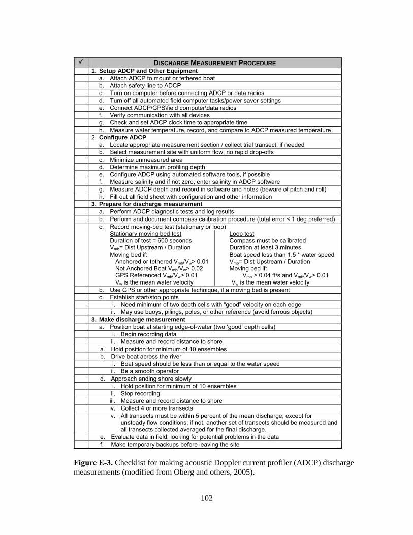
102

DISCHARGE MEASUREMENT PROCEDURE 1. Setup ADCP and Other Equipment a. Attach ADCP to mount or tethered boat b. Attach safety line to ADCP c. Turn on computer before connecting ADCP or data radios d. Turn off all automated field computer tasks/power saver settings e. Connect ADCP\GPS\field computer\data radios f. Verify communication with all devices g. Check and set ADCP clock time to appropriate time h. Measure water temperature, record, and compare to ADCP measured temperature 2. Configure ADCP a. Locate appropriate measurement section / collect trial transect, if needed b. Select measurement site with uniform flow, no rapid drop-offs c. Minimize unmeasured area d. Determine maximum profiling depth e. Configure ADCP using automated software tools, if possible f. Measure salinity and if not zero, enter salinity in ADCP software g. Measure ADCP depth and record in software and notes (beware of pitch and roll) h. Fill out all field sheet with configuration and other information 3. Prepare for discharge measurement a. Perform ADCP diagnostic tests and log results b. Perform and document compass calibration procedure (total error < 1 deg preferred) c. Record moving-bed test (stationary or loop) Stationary moving bed test

Duration of test = 600 seconds Vmb= Dist Upstream / Duration Moving bed if:

Anchored or tethered Vmb/Vw> 0.01 Not Anchored Boat Vmb/Vw> 0.02 GPS Referenced Vmb/Vw> 0.01 Vw is the mean water velocity

Loop test Compass must be calibrated Duration at least 3 minutes Boat speed less than 1.5 * water speed Vmb= Dist Upstream / Duration Moving bed if:

Vmb > 0.04 ft/s and Vmb/Vw> 0.01 Vw is the mean water velocity

b. Use GPS or other appropriate technique, if a moving bed is present c. Establish start/stop points i. Need minimum of two depth cells with “good” velocity on each edge ii. May use buoys, pilings, poles, or other reference (avoid ferrous objects) 3. Make discharge measurement a. Position boat at starting edge-of-water (two ‘good’ depth cells) i. Begin recording data ii. Measure and record distance to shore a. Hold position for minimum of 10 ensembles b. Drive boat across the river i. Boat speed should be less than or equal to the water speed ii. Be a smooth operator d. Approach ending shore slowly i. Hold position for minimum of 10 ensembles ii. Stop recording iii. Measure and record distance to shore iv. Collect 4 or more transects v. All transects must be within 5 percent of the mean discharge; except for

unsteady flow conditions; if not, another set of transects should be measured and all transects collected averaged for the final discharge.

e. Evaluate data in field, looking for potential problems in the data f. Make temporary backups before leaving the site

Figure E-3. Checklist for making acoustic Doppler current profiler (ADCP) discharge measurements (modified from Oberg and others, 2005).

103

APPENDIX F – MEASUREMENT REVIEW PROCEDURES Teledyne RD Instruments ADCP

1. Load Data • Load measurement file (File-Open

Measurement – Ctrl-O) • Select transect and Reprocess Transect

(Shift-F5)

2. Check Ship Stick Plots • Look at ship stick plot • Verify velocity reference (BT or GGA) • Step through depths using ↓ (if problems

are observed, look at velocity contour plots or intensity / back scatter plots)

3. Velocity Magnitude Contour • Review velocity magnitude contour. • Scale as appropriate. • Look for bad or missing data, bed

contour, lost ensembles, etc.)

4. Composite Tabular.—Review: • Number of Ensembles (total) vs:

(1) Bad ensembles (2) Lost ensembles

• What is value for % Bad bins? • Is water temperature realistic? • Do the edge discharges appear

reasonable? • Do edge discharges have correct signs?

5. System Parameters • Hit F9 to check system parameters • Does the info there (Frequency,

Firmware, Water and Bottom modes, Cell Size) match the direct commands (F3) specified in the config file?

• Does it match the field sheet?

104

6. Projected Velocity Contour • Hit F2 to set angle for projected velocity

contour plot and verify that value for the angle is correct. “Freeze” that value (for the first transect – assuming that flow is uni-directional).

• View-Graph-Contour Velocity – select Earth Projected Velocity data

• Scale as appropriate • Look for reverse / bi-directional flow

7. Error Velocity • View-Graph-Contour Velocity – select

Earth Error Velocity data Scale properly • Look for ambiguity errors, 3-beam

solutions. Outliers can be related to ambiguity errors or turbulence.

8. Configuration – Direct Commands • Press F3 and check direct commands

(Wizard and User) • Was the Config Wizard used? • Are the Wizard and User commands set

correctly for ADCP and flow conditions?

9. Configuration – DS/GPS • Check to see if Depth sounder used

10. Configuration – Discharge • Are extrapolation methods correct? • Review edge types selected. • Were water profile bins cutoff? Why?

Is it documented? • Proper shore ensembles (10)?

11. Configuration – Edge Estimates

• Are Edge distances consistent w/ field sheet? If not, is explanation been supplied?

• Are Edge distances estimated rather than measured?

• Are the estimated edge discharges reasonable for this section?

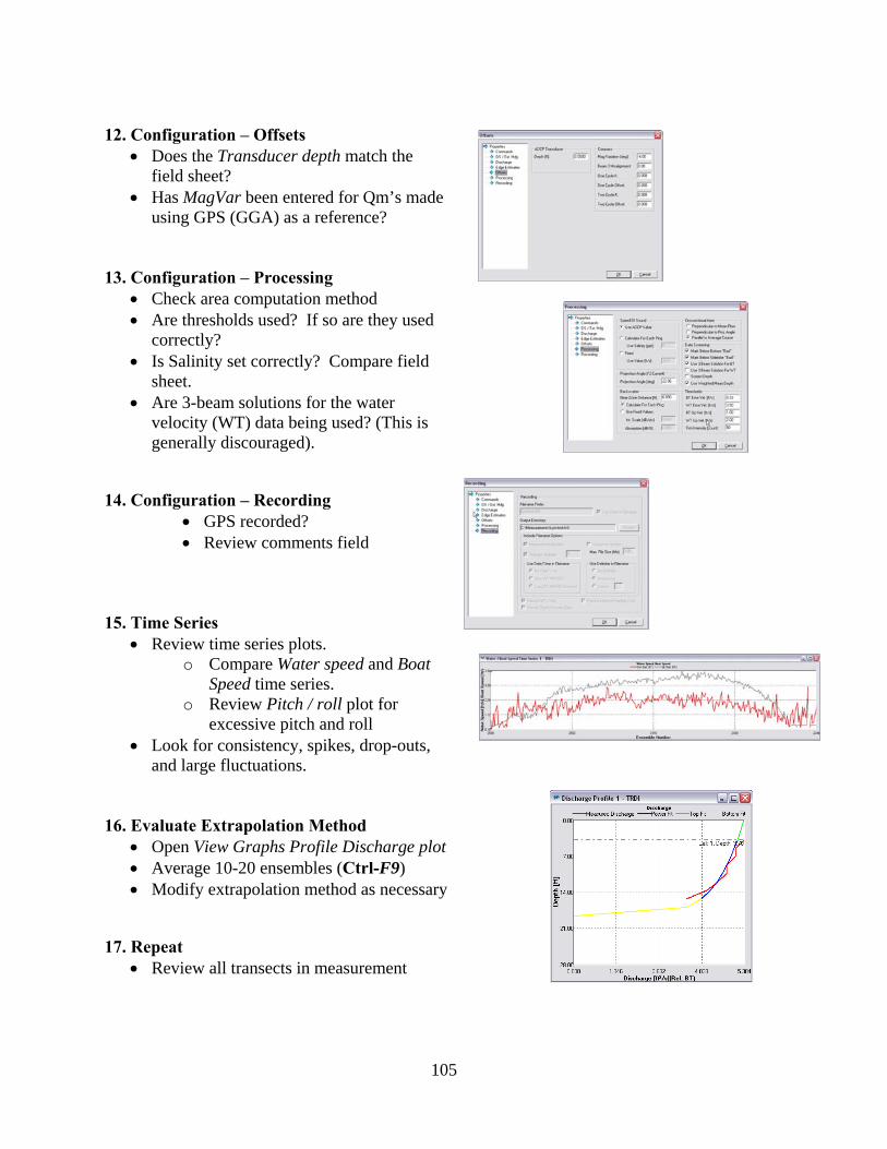
105

12. Configuration – Offsets

• Does the Transducer depth match the field sheet?

• Has MagVar been entered for Qm’s made using GPS (GGA) as a reference?

13. Configuration – Processing

• Check area computation method • Are thresholds used? If so are they used

correctly? • Is Salinity set correctly? Compare field

sheet. • Are 3-beam solutions for the water

velocity (WT) data being used? (This is generally discouraged).

14. Configuration – Recording • GPS recorded? • Review comments field

15. Time Series • Review time series plots.

o Compare Water speed and Boat Speed time series.

o Review Pitch / roll plot for excessive pitch and roll

• Look for consistency, spikes, drop-outs, and large fluctuations.

16. Evaluate Extrapolation Method • Open View Graphs Profile Discharge plot • Average 10-20 ensembles (Ctrl-F9) • Modify extrapolation method as necessary

17. Repeat • Review all transects in measurement

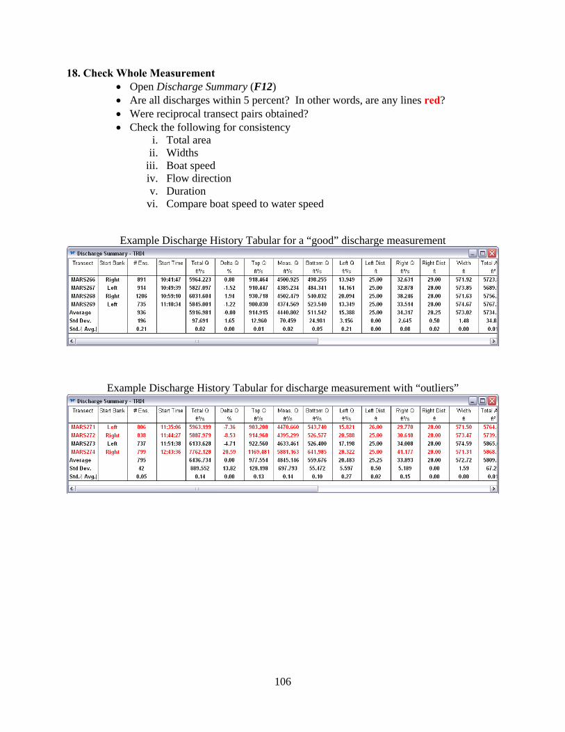
106

18. Check Whole Measurement • Open Discharge Summary (F12) • Are all discharges within 5 percent? In other words, are any lines red? • Were reciprocal transect pairs obtained? • Check the following for consistency

i. Total area ii. Widths

iii. Boat speed iv. Flow direction v. Duration

vi. Compare boat speed to water speed

Example Discharge History Tabular for a “good” discharge measurement

Example Discharge History Tabular for discharge measurement with “outliers”

107

Sontek/YSI ADP

1. Load Data

• Load measurement file (File-Open Measurement – Ctrl-O)

• Select transect and Reprocess Transect (Shift-F5)

2. Check Ship Plots

• Look at ship plot • Verify velocity reference (BT or GPS) • Step through depths (if problems are observed, look at velocity

contour plots or intensity / SNR plots)

3. Velocity Magnitude Contour • Review velocity magnitude

contour. • Scale as appropriate. • Look for bad or missing data,

bed contour, etc.)

4. Tabular Data: • Number of profiles

• What is value for % Bad bins? • Is water temperature realistic? • Do the edge discharges appear reasonable? • Do edge discharges have correct signs?

5. Velocity Direction Contour

• View-Contour Control Box – select Velocity and Direction data • Scale as appropriate • Look for reverse / bi-directional flow

108

6. Configuration

• Press CNTR-U and check configuration • Check bin size, range, blank • Does the Transducer depth match the field

sheet? • Has MagVar been entered for Qm’s made

using GPS as a reference?

7. Velocity Profile Extrapolation • Select Processing – Velocity Profile

Extrapolation • Right-click on profile graph and select profile

extrapolation. • Are extrapolation methods correct? • Review edge types selected. • Were water profile bins cutoff? Why? Is it

documented?

8. Time Series • Review time series plots. • Right-click on the y-axis of the bar chart and

select the appropriate variable. • Compare Water speed and Boat Speed time

series. • Review pitch and roll plot for excessive

pitch and roll • Look for consistency, spikes, drop-outs,

and large fluctuations.

9. Discharge Computation

• Select Processing – Discharge Calculation • Are Edge distances consistent w/ field sheet? If

not, is explanation been supplied? • Are Edge distances estimated rather than

measured? • Are the estimated edge discharges reasonable for

this section? • Recompute discharge • Check for consistency and reasonableness

109

10. Repeat • Review all transects in measurement

11. Check Whole Measurement • Select File – Discharge Summary or Cntrl-Y • Are all discharges within 5 percent? • Were reciprocal transect pairs obtained? • Check the following for consistency

o Total area o Widths o Boat speed o Flow direction o Duration o Compare boat speed to water speed

Best Practices for Measuring Discharge with Acoustic ... · 1 Best Practices for Measuring...

Documents

Transcript of Best Practices for Measuring Discharge with Acoustic ... · 1 Best Practices for Measuring...