Best estimate of debt risk premium for the 16 November to 4 December 2015 period

Dr. Tom Hird

February 2016

i

Table of Contents

1 Introduction 1

2 Obtaining spread to swap estimates 4

2.1 Extrapolation beyond 10 years 4

2.2 Bloomberg BVAL curve 4

2.3 RBA curve 4

2.4 Reuters curve 6

2.5 Summary 7

3 Methodology for comparing estimates 9

3.1 Goodness-of-fit tests 9

3.2 Nelson-Siegel estimates 19

3.3 Conclusion 20

Appendix A Curves with BVAL shape beyond 10 years 22

Appendix B Updated memorandum on the cost of debt under different

debt management strategies 24

B.1 Purpose 24

B.2 Cost of debt 24

B.3 Inflation 25

B.4 16 Nov 2015 – 4 Dec 2015 swap values 26

B.5 Historical swap and DRP values 27

Appendix C Terms of reference 28

Appendix D Curriculum vitae 37

Contact Details 37

ii

iii

List of Figures

Figure 1: Spreads from BVAL, RBA-AER, RBA-SAPN, and Reuters curves (semi-

annual) .................................................................................................................. 8

Figure 2: Broad sample by currency of issue (semi-annual) .............................................. 12

Figure 3: Broad sample by credit rating (semi-annual) ...................................................... 12

Figure 4: RBA sample by currency of issue (semi-annual) ................................................. 13

Figure 5: RBA sample by credit rating (semi-annual) ........................................................ 13

Figure 6: BVAL sample by currency of issue (semi-annual) ............................................... 14

Figure 7: BVAL sample by credit rating (semi-annual) ...................................................... 14

Figure 8: Reuters sample by currency of issue (semi-annual) ........................................... 15

Figure 9: Reuters sample by credit rating (semi-annual) ................................................... 15

iv

List of Tables

Table 1: Yield and DRP estimates (BVAL, RBA-AER, RBA-SAPN, Reuters, semi-

annual) 1

Table 2: Average spread to swap estimates (16 Nov 2015 – 4 Dec 2015, semi-annual) 8

Table 3: Distribution of bonds in broad sample 10

Table 4: Distribution of bonds in RBA sample 10

Table 5: Distribution of bonds in BVAL sample 11

Table 6: Distribution of bonds in Reuters sample 11

Table 7: Goodness-of-fit tests – weighted sum of squared residuals (semi-annual) 17

Table 8: Difference between spread to swap curve estimates compared to the

Nelson-Siegel 10-year estimate (semi-annual) 20

Table 9: Goodness-of-fit tests – weighted sum of squared residuals (curves with

BVAL shape beyond 10 years) (semi-annual) 23

Table 10: Cost of debt allowance in year 1 (AER extrapolation in all periods,

annualised) 25

Table 11: Break-even (and actual) inflation estimates (averaged over 16 November

2015 to 11 December 2015) 26

Table 12: Daily swap rates over 16 November 2015 to 4 December 2015 by maturity

(semi-annual) 27

Table 13: Historical DRPs (measured to swap values, semi-annual) 27

1

1 Introduction 1. Jemena Electricity Network (JEN) proposed an averaging period that spans the 15

trading days from 16 November 2015 to 4 December 2015. We have been asked to

provide an analysis of the goodness of fit to the data of available independent

published estimates of BBB corporate yields.1 Based on our conclusions, we have

also been asked to update our 5 January memo estimating the cost of debt under

different debt management strategies (which we do in Appendix B to this report).

We have considered the following four sources of debt risk premium (DRP)2

estimates:

a. Bloomberg’s AUD BBB BVAL curve (BVCSAB3M Index – BVCSAB30

Index)(BVAL);

b. RBA’s BBB spread to swap Gaussian kernel (RBA statistics table F3),

extrapolated to a 10-year effective tenor using the Australian Energy

Regulator’s (AER’s) extrapolation method (RBA-AER);

c. RBA’s BBB spread to swap Gaussian kernel, extrapolated using the SA

PowerNetworks (SAPN) extrapolation method (RBA-SAPN); and

d. Reuters’ AUD BBB par yield curve (FNFSBBB3M – FNFSBBB10M).3

2. The four sets of yield and DRP estimates are shown in Table 1, for the 16 November

2015 – 4 December 2015 averaging period:

Table 1: Yield and DRP estimates (BVAL, RBA-AER, RBA-SAPN, Reuters, semi-annual)

Averaging period Type 10-year swap

(Bloomberg)

BVAL RBA AER RBA SAPN Reuters

16 Nov 2015 – 4 Dec 2015

Yield 302.10 554.15 555.39 559.57 585.95

Spread - 252.05 253.29 257.47 283.85

Source: RBA, Bloomberg, Reuters, CEG analysis;

1 Terms of reference are provided in Appendix C, and Dr Tom Hird’s CV is shown in Appendix D.

2 We define the DRP in this report as the spread between the yield and the swap rate of the same term to

maturity.

3 Although Reuters has its own set of DRP estimates, we obtained the Reuters DRP using the difference

between Reuters’ par yield curve and Bloomberg’s swap rates for consistency with our other DRP

estimates which are all calculated by subtracting Bloomberg swap rates from published yields.

2

3. We have provided an assessment for each of the four sources in a separate report,4

in which we also suggested applying goodness-of-fit tests to a broad sample of

bonds in order to identify which estimate should be used.5 In that report, we noted

that if a single curve was to be selected without recourse to empirical testing in a

specific averaging period then it would be appropriate to rely exclusively, or at least

most heavily, on the RBA curve. However, we also noted that, in any given

averaging period, empirical analysis could be performed in order to select which

curve, or combination of curves, provided the best fit to the data. This report

performs such analysis in JEN’s averaging period.

4. In contrast, the AER’s preferred approach is to take the simple average of the BVAL

and RBA curve with AER extrapolation (RBA-AER) 10-year cost of debt estimates.

5. This report utilises two approaches to identify the best estimate of the DRP to be

used for calculating the benchmark rate of return:

a. Goodness-of-fit tests compared to the broad sample of bonds, the RBA sample,

and the Bloomberg sample; and

b. Comparison against the 10-year estimate from the Nelson-Siegel curve fitted on

the spreads to swap of the broad sample of bonds.6

6. We conducted both analyses against the four DRP curves over JEN’s proposed

averaging period, as well as for the averages of the following subsets of the four

curves:7

RBA-AER and BVAL (AER’s preferred approach);

RBA curve with SAPN extrapolation (RBA-SAPN) and BVAL;

RBA-AER and Reuters;

RBA-SAPN and Reuters;

Reuters and BVAL;

RBA-AER, BVAL, and Reuters; and

4 CEG, Criteria for assessing fair value curves, January 2016.

5 The procedure for applying goodness-of-fit tests was set out in: CEG, Critique of the AER’s JGN draft

decision on the cost of debt, April 2015.

6 As with the goodness-of-fit approach, the Nelson-Siegel approach was also put forward in: CEG, Critique

of the AER’s JGN draft decision on the cost of debt, April 2015.

7 To be clear, we consider three sources of DRP – BVAL, RBA, and Reuters. The RBA curve can be

extrapolated in two ways, which leads to four DRP curves in total – BVAL, RBA-AER, RBA-SAPN, and

Reuters. In addition to the 10-year DRP estimates from each of the four curves, we also evaluate a

further seven DRP estimates, derived as the simple average of a combination of two or more curves,

resulting in eleven DRP estimates.

3

RBA-SAPN, BVAL, and Reuters.

7. I acknowledge that we have read, understood and complied with the Federal Court

of Australia’s Practice Note CM 7, “Expert Witnesses in Proceedings in the Federal

Court of Australia”. I have made all inquiries that I believe are desirable and

appropriate to answer the questions put to me. No matters of significance that I

regard as relevant have to my knowledge been withheld.

8. I have been assisted in the preparation of this report by Johnathan Wongsosaputro

in CEG’s Sydney office. However, the opinions set out in this report are my own.

Thomas Nicholas Hird

4

2 Obtaining spread to swap estimates

2.1 Extrapolation beyond 10 years

9. The RBA and Reuters curves only publish yield estimates up to 10 years. Beyond 10

years we have extrapolated these curves linearly. That is, we have assumed the

same rate of change in spread to swap beyond 10 years as exists between the 10 year

data point and the data point immediately preceding 10 years. We also present in

Appendix A the results if we assume that RBA and Reuters curves have the same

slope shape beyond 10 years as the Bloomberg BVAL curve (the only curve that

extends beyond 10 years).

2.2 Bloomberg BVAL curve

10. Yield estimates of the AUD BBB BVAL curve are available for tenors ranging from 3

months (BVCSAB3M Index) to 30 years (BVCSAB30 Index). However, Bloomberg’s

swap rates are only available from 1 year (ADSWAP1 Curncy) onwards. We

therefore did not include BVAL curve data at the 3-month and 6-month tenors in

our analysis.

11. Furthermore, since the RBA and Reuters curves only extend to 10 years, in order to

have consistent assessment across all curves we have applied two approaches.

First, we include data from the full BVAL curve up to the 30-year tenor, and

linearly extrapolate all other curves beyond 10 years based on the shape of the

curves between 10 years and the maturity closest to (but below) 10 years

(Section 3.1.3);

Second, we also present results where we assume that all curves have the same

shape as the BVAL curve beyond 10 years (Appendix A).

12. The BVAL yields are then converted into spreads to swap by deducting the swap

rates at the corresponding tenors.

2.3 RBA curve

13. The RBA provides on-the-day estimates of yields, spreads to CGS, spreads to swap,

and effective tenors at the end of each month for the 3, 5, 7, and 10 year target

tenors. Since the RBA’s approach results in estimates with effective tenors that are

5

less than their corresponding target tenors, the RBA estimates have to be

extrapolated to achieve an effective tenor of 10 years.8

14. In its recent decisions, the AER has considered two methods for extrapolating the

RBA curve to an effective tenor of 10 years. These are referred to as the AER and

SAPN methods, both of which are considered in our analysis.

2.3.1 AER extrapolation

15. Under the AER extrapolation method, the RBA yield curve is extrapolated to 10

years using linear interpolation of the 7- and 10-year spread to swap estimates. This

is carried out using the following formula:

10 𝑦𝑒𝑎𝑟 𝑒𝑓𝑓𝑒𝑐𝑡𝑖𝑣𝑒 𝑦𝑖𝑒𝑙𝑑

= 10 𝑦𝑒𝑎𝑟 𝑡𝑎𝑟𝑔𝑒𝑡 𝑦𝑖𝑒𝑙𝑑 + (10 𝑦𝑒𝑎𝑟 𝑡𝑎𝑟𝑔𝑒𝑡 𝑠𝑝𝑟𝑒𝑎𝑑 − 7 𝑦𝑒𝑎𝑟 𝑡𝑎𝑟𝑔𝑒𝑡 𝑠𝑝𝑟𝑒𝑎𝑑)

× (10 − 𝑒𝑓𝑓𝑒𝑐𝑡𝑖𝑣𝑒 𝑡𝑒𝑛𝑜𝑟 𝑜𝑓 10 𝑦𝑒𝑎𝑟 𝑡𝑎𝑟𝑔𝑒𝑡)

(𝑒𝑓𝑓𝑒𝑐𝑡𝑖𝑣𝑒 𝑡𝑒𝑛𝑜𝑟 𝑜𝑓 10 𝑦𝑒𝑎𝑟 𝑡𝑎𝑟𝑔𝑒𝑡 − 𝑒𝑓𝑓𝑒𝑐𝑡𝑖𝑣𝑒 𝑡𝑒𝑛𝑜𝑟 𝑜𝑓 7 𝑦𝑒𝑎𝑟 𝑡𝑎𝑟𝑔𝑒𝑡)

2.3.2 SAPN extrapolation

16. Under the SAPN extrapolation method, the RBA yield curve is extrapolated to 10

years based on the regression slope of the 3- to 7-year spread to swap estimates.

This is carried out using the following formula:

10 𝑦𝑒𝑎𝑟 𝑒𝑓𝑓𝑒𝑐𝑡𝑖𝑣𝑒 𝑦𝑖𝑒𝑙𝑑

= 10 𝑦𝑒𝑎𝑟 𝑡𝑎𝑟𝑔𝑒𝑡 𝑦𝑖𝑒𝑙𝑑 + 3 𝑡𝑜 10 𝑦𝑒𝑎𝑟 𝑠𝑙𝑜𝑝𝑒 × (10

− 𝑒𝑓𝑓𝑒𝑐𝑡𝑖𝑣𝑒 𝑡𝑒𝑛𝑜𝑟 𝑜𝑓 10 𝑦𝑒𝑎𝑟 𝑡𝑎𝑟𝑔𝑒𝑡)

17. The 3 to 10 year slope in the equation above is obtained by regressing the yield

estimates at the 3, 5, 7, and 10 year target tenor, against their corresponding

effective tenors.

2.3.3 Interpolating to obtain daily data

18. Having extrapolated the RBA yield curve to an effective tenor of 10 years using the

AER and SAPN methods, the estimates are then interpolated to a daily frequency

using the following steps:

i. Calculate daily effective tenors for the 3, 5, 7, and 10 year targets by linearly

interpolating between estimates from the two closest months.

8 The RBA uses a Gaussian kernel to derive their DRP estimates, whereby more weight is assigned to the

spreads of the bonds that are closer to the target tenor. Since the RBA sample generally contains more

bonds with residual maturities below 10 years, the Gaussian kernel approach results in a 10-year

estimate with an effective tenor that is also less than 10 years. Extrapolation is thus necessary in order to

obtain an estimate that is more accurate at the 10-year tenor.

6

ii. Calculate daily CGS yields using linear interpolation of on-the-day yields of CGS

bonds, obtained from RBA statistical table F16.9 These are calculated for the

effective tenors at the 3, 5, 7, and 10 year targets obtained in (i), as well as the

10-year effective tenor.

iii. Calculate end-of-month spreads to CGS by deducting the corresponding CGS

yields calculated in (ii) from the RBA’s 3, 5, 7, and 10 year target yields and the

extrapolated 10-year yield.10

iv. Convert the end-of-month spreads to CGS obtained in (iii) into daily spreads to

CGS by linearly interpolating between the estimates from the two closest

months.

v. Calculate daily yields as the sum of the daily CGS yields obtained in (ii) and the

daily spreads to CGS obtained in (iv).

vi. Calculate daily spreads by interpolating the daily Bloomberg swap rates for the

effective tenors at the 3, 5, 7, and 10 year targets obtained in (i), as well as the

10-year effective tenor.

vii. Obtain the daily series of spreads to swap by deducting the interpolated daily

Bloomberg swap rates obtained in (vi) from the daily yields obtained in (v).

19. When converting the month-end spreads to daily spreads, the above steps carry out

interpolation on the spreads to CGS as opposed to the spreads to swap. This is

necessary because the RBA publishes a daily series of yields on CGS bonds, but does

not publish a daily series for swap rates. As such, the month-end spreads to swap

cannot be interpolated directly to a daily frequency since doing so would result in a

yield series that does not accurately reflect the daily movements in between months.

20. The above steps result in two series of spread to swap curves, which are obtained by

using two different extrapolation methods in step (ii). We denote these as the RBA-

AER and RBA-SAPN curves.

2.4 Reuters curve

21. Reuters publishes daily estimates for an AUD BBB par yield curve, a zero yield

curve, and a swap spread curve. For this analysis, the Reuters spread to swap curve

is obtained by deducting Bloomberg swap rates from the Reuters par yield curve.

9 RBA, Indicative Mid Rates of Australian Government Securities – 2013 to Current – Table F16.

10 The extrapolated 10-year yield can be calculated using the AER and SAPN extrapolation methods.

7

22. We used the Reuters par yield curve instead of the ‘zero’ (zero coupon)11 yield curve

because we consider the former to be a more appropriate comparison to the BVAL

and RBA curves – both of which are the yields on coupon paying bonds. The zero

yield curve is higher than the par yield curve reflecting the fact that a bond that has

lower coupons will have a longer effective maturity (or ‘duration’). When the yield

curve is upward sloping (as it typically is especially for risky bonds and was over

JEN’s averaging period) this implies that the yield on a zero coupon bond will be

higher because its effective maturity is higher. Put simply, zero coupon bonds

require investors to wait longer for their return and they typically demand a higher

return for doing so.

23. We note that the operation of the PTRM is such that it backloads the effective

compensation for the cost of debt (and equity). Specifically, instead of providing

sufficient cash-flow to pay the nominal cost of debt input into the PTRM it only

provides enough cash-flow to pay the real (inflation adjusted) cost of debt. The

compensation for the cost of inflation is provided in the form of a higher RAB

(which raises cash-flows over future regulatory periods). On this basis, the

appropriate yield curve to use that mimics the timing assumptions in the PTRM is

likely to be between the par yield and zero yield curve. Consequently, our use of the

coupon paying curves results in a conservative estimate, such that the resulting

spread to swap is likely to be underestimated.

2.5 Summary

24. The methods set out in Sections 2.1 to 2.4 generate four daily spread to swap curve

estimates. The average spreads for the 16 November 2015 to 4 December 2015

averaging period are shown in Table 2 and Figure 1.

11 The zero yield to maturity of a bond paying zero coupons.

8

Table 2: Average spread to swap estimates (16 Nov 2015 – 4 Dec 2015, semi-annual)

Target tenor

1 2 3 4 5 6 7 8 9 10 Extrap (to 10 years)

BVAL 113.3 133.1 160.0 201.7 208.2 225.1 234.8 245.2 252.1

RBA-AER*

227.8 247.1 260.7 255.3 253.3

RBA-SAPN*

227.8 247.1 260.7 255.3 257.5

RBA effective tenors

3.8 5.0 6.6 9.2 10.0

Reuters 116.1 194.2 213.2 200.4 190.2 196.0 211.6 233.2 257.7 283.9

Source: Bloomberg, RBA, SAPN, CEG analysis; *The spreads of the RBA-AER and RBA-SAPN curves are

plotted with reference to their effective tenors. For example, the estimate of 255.3 basis points corresponds to a

9.2 year tenor on both RBA curves. The last column of the table therefore represents the 10-year estimates of the

RBA-AER and RBA-SAPN curves, and these are analogous to the 10-year estimates of the BVAL and Reuters

curves as shown in the second-to-last column from the right.

Figure 1: Spreads from BVAL, RBA-AER, RBA-SAPN, and Reuters curves (semi-annual)

Source: Bloomberg, RBA, Reuters, CEG analysis

9

3 Methodology for comparing estimates

25. The spread to swap estimates shown in Table 2 above are compared using two

methods:

Goodness of fit tests compared to the broad sample proposed in CEG (2015),12

the RBA sample, and the BVAL sample;13 and

Comparison to the 10-year estimate of the Nelson-Siegel curve.

3.1 Goodness-of-fit tests

26. We obtain the daily yields of the bonds in each of the samples over the averaging

period from Bloomberg, before converting them to AUD fixed equivalent spreads to

swap using the method utilised by the RBA.14 In particular, for comparability

purposes, the yields of bonds in the Reuters sample were also sourced from

Bloomberg.

27. The goodness-of-fit tests are then carried out by calculating the weighted sum of

squared residuals (SSR), in which the spreads to swap of each bond in the selected

sample are compared against the estimates from each curve.15 As with the

methodology used in CEG (2015), the squared residuals are weighted according to

the difference between the bond’s residual maturity and the 10-year target tenor,

measured using a Gaussian kernel with a standard deviation of 1.5 years.16 We also

carry out an alternative analysis in which the weights are based on the Gaussian

kernel and the AUD issue amount of the bond. This alternative weighting gives

more weight to larger issues and is appropriate if it is believed that the estimated

yields on larger issues are more likely to accurately reflect the benchmark (e.g., if it

is believed that these bonds are more liquid and therefore more likely to have

accurate prices).17

12 CEG, Critique of the AER’s JGN draft decision on the cost of debt, April 2015.

13 We use the RBA’s December 2015 sample, which consists of 93 bonds. The BVAL sample has between 21

and 23 bonds on each day over the averaging period, and we include all bonds that appeared at least

once during the period, resulting in a sample of 25 bonds.

14 RBA, New Measures of Australian Corporate Credit Spreads, December 2013.

15 A lower sum of squared residuals means that a curve provides a better fit to the spreads to swap of the

bonds in the selected sample, and vice versa.

16 This is the same standard deviation parameter that the RBA uses in its Gaussian kernel.

17 Lally criticised the inclusion of low value bonds in the broad sample, on the basis that they tended to be

illiquid and thus had lower data quality. This alternative weighting resolves that issue by giving lower

10

28. Based on this analysis, the curve that corresponds to the smallest weighted sum of

squared residuals provides the best fit to the chosen sample, which would suggest

that its estimate is the most appropriate.

3.1.1 Bond samples

29. The range of residual maturities, credit ratings, and currency of issue for each

sample are shown in Table 3 to Table 6. Scatterplots of each sample are shown in

Figure 2 to Figure 9, separated according to currency of issue and credit rating.18

Table 3: Distribution of bonds in broad sample

S&P rating Total

BBB- BBB BBB+

39 69 82 190

Maturity (yr)

0-4 4-6 6-8 8-12 12+

70 56 21 30 13 190

Currency

AUD USD EUR GBP

114 50 19 7 7 190

Source: Bloomberg, CEG analysis

Table 4: Distribution of bonds in RBA sample

S&P rating Total

BBB- BBB BBB+ Other*

23 34 33 3 93

Maturity (yr)

0-4 4-6 6-8 8-12 12+

33 33 12 11 4 93

Currency

AUD USD EUR GBP

46 32 15 0 93

Source: Bloomberg, RBA, CEG analysis; *3 of the bonds were issued by APT Pipelines and had no S&P credit

rating, but all 3 had issuer credit ratings listed as BBB

weights to bonds with low value. See: Lally, Review of submissions on implementation issues for the cost

of debt, October 2015, pg 10.

18 In the credit rating charts, “other” refers to the 3 APT Pipeline bonds with no S&P bond credit rating but

with S&P issuer credit rating listed as BBB. The purple glow in Figure 3 to Figure 9 is used to highlight

the location of the RBA-AER curve, which is behind the RBA-SAPN curve for the 3.8- to 9.2-year

maturities.

11

Table 5: Distribution of bonds in BVAL sample

S&P rating Total

BBB- BBB BBB+

6 9 7 22

Maturity (yr)

0-4 4-6 6-8 8-12 12+

16 4 1 1 0 22

Currency

AUD USD EUR GBP

22 0 0 0 22

Source: Bloomberg, CEG analysis

Table 6: Distribution of bonds in Reuters sample

S&P rating Total

BBB- BBB BBB+ Other*

8 10 22 5 45

Maturity (yr)

0-4 4-6 6-8 8-12 12+

27 14 3 1 0 45

Currency

AUD USD EUR GBP

45 0 0 0 45

Source: Bloomberg, Reuters, CEG analysis; *1 bond (EK8989288 Corp) is rated A- by S&P, A3 by Moody’s, and

BBB+ by Fitch. The remaining 4 bonds have no S&P ratings but possess ratings by Moody’s and/or Fitch.

12

Figure 2: Broad sample by currency of issue (semi-annual)

Source: Bloomberg, RBA, Reuters, CEG analysis

Figure 3: Broad sample by credit rating (semi-annual)

Source: Bloomberg, RBA, Reuters, CEG analysis

13

Figure 4: RBA sample by currency of issue (semi-annual)

Source: Bloomberg, RBA, Reuters, CEG analysis

Figure 5: RBA sample by credit rating (semi-annual)

Source: Bloomberg, RBA, Reuters, CEG analysis

14

Figure 6: BVAL sample by currency of issue (semi-annual)

Source: Bloomberg, RBA, Reuters, CEG analysis

Figure 7: BVAL sample by credit rating (semi-annual)

Source: Bloomberg, RBA, Reuters, CEG analysis

15

Figure 8: Reuters sample by currency of issue (semi-annual)

Source: Bloomberg, RBA, Reuters, CEG analysis; *Bond yields sourced from Bloomberg

Figure 9: Reuters sample by credit rating (semi-annual)

Source: Bloomberg, RBA, Reuters, CEG analysis; *Bond yields sourced from Bloomberg

16

3.1.2 Combinations of curves

30. The AER’s preferred methodology for deriving the benchmark DRP is to take the

simple average of the 10-year AUD BBB BVAL spread to swap and the 10-year

extrapolated AUD BBB RBA-AER spread to swap.

31. We therefore also carry out goodness-of-fit tests on the averages of the BVAL and

RBA-AER curves, as well as other combinations of averages:

50% BVAL, 50% RBA-AER (AER’s preferred estimate);

50% BVAL, 50% RBA-SAPN;

50% RBA-AER, 50% Reuters;

50% RBA-SAPN, 50% Reuters;

50% BVAL, 50% Reuters;

33.3% BVAL, 33.3% RBA-AER, 33.3% Reuters; and

33.3% BVAL, 33.3% RBA-SAPN, 33.3% Reuters.

32. When constructing the average curves listed above, linear interpolations were used

if the estimate for one of the curves was not available at a particular tenor. For

example, since the BVAL curve does not include an estimate for the 6 year tenor, we

interpolated between the 5 and 7 year estimates to obtain a BVAL input into the

respective curve combinations.

3.1.3 Test results

33. The results of these goodness-of-fit tests are shown in Table 7, where we report the

weighted sum of squared residuals divided by the number of bonds in the sample.

17

Table 7: Goodness-of-fit tests – weighted sum of squared residuals (semi-annual)

Sources DRP estimate

SSR divided by # of bonds; Gaussian kernel and AUD amount issued as weights

SSR divided by # of bonds; Gaussian kernel weights

BVAL RBA-AER

RBA-SAPN

Reuters Broad RBA (Dec 2015

sample)

BVAL (16 Nov – 4 Dec

2015)

Reuters (14 Dec 2015 sample)

Broad RBA (Dec 2015

sample)

BVAL (16 Nov – 4 Dec

2015)

Reuters (14 Dec 2015 sample)

100% 252.05 10.33 23.77 13.75 21.02 16.10 30.38 13.66 17.89

100% 253.29 10.92 23.67 13.58 37.19 16.63 29.41 8.69 29.24

100% 257.47 11.03 23.85 13.18 37.02 17.44 29.74 8.29 29.06

100% 283.85 15.60 31.51 18.25 17.93 26.48 41.03 20.04 16.66

50% 50% 252.67 10.37 23.18 11.61 27.18 16.06 29.19 9.25 21.81

50% 50% 254.76 10.41 23.24 11.19 27.00 16.45 29.32 8.82 21.63

50% 50% 268.57 11.81 25.40 9.70 22.61 20.01 32.77 8.48 18.38

50% 50% 270.66 12.19 25.89 10.00 22.74 20.73 33.31 8.79 18.51

50% 50% 267.95 11.77 25.87 10.75 16.98 20.10 34.00 11.61 14.78

33.3% 33.3% 33.3% 262.80 11.00 24.32 9.19 21.22 18.38 31.44 8.33 17.34

33.3% 33.3% 33.3% 264.19 11.17 24.54 9.17 21.21 18.79 31.71 8.32 17.34

Source: Bloomberg, RBA, Reuters, CEG analysis

18

34. The lowest sum of squared errors in each column is highlighted yellow. The lowest

sum of squared errors in each subset19 of each column is highlighted green (if

different to the lowest sum of squared errors overall). The grey highlighting is

provided for ease of comparison to the average of all three curves.

35. The results show that there is little to distinguish between the BVAL, RBA-AER, and

RBA-SAPN curves when evaluated individually against the broad sample and their

respective samples. Among these three curves, BVAL has the lowest weighted SSR

for the broad sample, RBA-AER has the lowest for the RBA sample, and RBA-SAPN

has the lowest for the BVAL sample. In most cases, the difference between the

lowest and highest weighted SSR divided by the number of bonds is very small.

36. In contrast, the Reuters curve performs relatively poorly across all samples other

than its own, with average weighted sum of squared residuals that exceed those

associated with the other three samples. We note, however, that this does not

automatically mean that no weight should be assigned to the Reuters curve. This is

because a linear combination of correlated estimates could still result in a better fit

– even if one of the estimates had a worse fit than the others – by virtue of the

correlations among the candidate curves.

37. Notably, Lally’s (2014) MSE estimate, which was also considered by the AER, is

based on a similar concept.20 To see this, consider two unbiased estimators, with

one estimator having a larger variance than the other.21 Depending on the

correlations between the two sets of estimation errors, taking a linear combination

of the two series could result in an estimator with even lower variance. This is

because the residuals of both series can have a cancelling effect on each other, with

a large residual for one series being mitigated by a smaller residual in the other, or

even a residual of the opposite sign. Combining these two series would then result in

a lower variance of residuals.

38. Turning to the curve combinations, it can once again be seen that no particular

combination appears to outperform the others substantially. No single combination

generates the lowest weighted sum of squared residuals over all 8 measures (4

samples × 2 different weighting schemes).

19 With one subset relating to 100% weight to different curves and the other subset relating to averages

across the curves.

20 Lally, Implementation issues for the cost of debt, November 2014.

21 In CEG (2016), we noted that Lally’s assumption about the two series being unbiased was highly

questionable since the Bloomberg sample did not provide an accurate reflection of the bond issuance

characteristics of a BEE. Although our view on this issue has not changed, our analysis here nevertheless

explores how the results would change if the assumption of unbiasedness did hold true for all the

sources of estimates.

19

3.2 Nelson-Siegel estimates

39. The Nelson-Siegel curve is commonly used to estimate yield curves from a sample of

bonds. The Nelson-Siegel curve was proposed by CEG (2015) and elsewhere as a

method for choosing between estimates.22

40. As discussed in previous CEG reports,23 the Nelson Siegel curve estimation

technique is the dominant methodology used by finance researchers to estimate

yield curves. It is therefore relevant to ask how each of the estimates compares to

this finance industry yardstick for estimation of benchmark yields.

41. The Nelson-Siegel curve takes on the following functional form:24

𝑦𝑡(𝜏) = 𝛽0𝑡 + 𝛽1𝑡

1 − 𝑒−𝜆𝜏

𝜆𝜏+ 𝛽2𝑡 (

1 − 𝑒−𝜆𝜏

𝜆𝜏− 𝑒−𝜆𝜏)

42. We have estimated this functional form using spread values as inputs. We estimate

the parameters of the Nelson-Siegel curve using Excel Solver’s GRG-Nonlinear

algorithm to minimise the sum of squared residuals compared to the bond yields in

each sample. As with the methodology in CEG (2015), we limit the maximum

residual maturities of bonds in the sample. This is necessary in order to minimise

the influence of bonds with very long maturities, since such bonds are high leverage

points and will heavily affect the shape of the curve even though they should

intuitively have less impact on the 10-year tenor of interest. We set a maximum

residual maturity of 30 years.

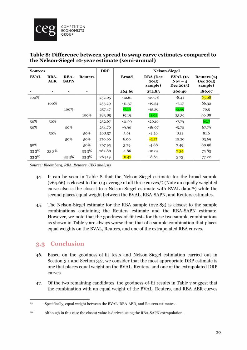
43. Table 8 shows the 10-year estimate of the Nelson-Siegel curve estimated using the

various samples, as well as the difference between source estimates compared to the

Nelson-Siegel estimate. We note that most weight should be given to the Nelson-

Siegel estimate derived using the broad sample (and to some extent the RBA

sample) because the larger sample size increases robustness of the regression

results. The estimates using the smaller BVAL/Reuters sample are likely to be less

robust but are provided for completeness.

22 CEG, Critique of the AER’s JGN draft decision on the cost of debt, April 2015. See also CEG, Cost of debt

consistent with the NGR and NGL, a report for ATCO, March 2014.

23 For example, see Appendix C of CEG (2015).

24 λ represents the exponential decay rate of the curve. Our estimation uses a starting value of λ = 0.7173.

The three β coefficients are dynamic factors. β0 represents the short-term factor; β1 the long-term factor;

and β2 the medium-term factor. In estimating the Nelson-Siegel curve, we imposed standard positivity

constraints on λ, β0, and β0 + β1. See: Diebold and Li (2006), Forecasting the term structure of

government bond yields, Journal of Econometrics, 130, pg 337-364.

20

Table 8: Difference between spread to swap curve estimates compared to the Nelson-Siegel 10-year estimate (semi-annual)

Sources DRP Nelson-Siegel

BVAL RBA-AER

RBA-SAPN

Reuters Broad RBA (Dec 2015

sample)

BVAL (16 Nov – 4

Dec 2015)

Reuters (14 Dec 2015 sample)

- - - - 264.66 272.83 260.46 186.97

100% 252.05 -12.61 -20.78 -8.41 65.08

100% 253.29 -11.37 -19.54 -7.17 66.32

100% 257.47 -7.19 -15.36 -2.99 70.5

100% 283.85 19.19 11.02 23.39 96.88

50% 50% 252.67 -11.99 -20.16 -7.79 65.7

50% 50% 254.76 -9.90 -18.07 -5.70 67.79

50% 50% 268.57 3.91 -4.26 8.11 81.6

50% 50% 270.66 6.00 -2.17 10.20 83.69

50% 50% 267.95 3.29 -4.88 7.49 80.98

33.3% 33.3% 33.3% 262.80 -1.86 -10.03 2.34 75.83

33.3% 33.3% 33.3% 264.19 -0.47 -8.64 3.73 77.22

Source: Bloomberg, RBA, Reuters, CEG analysis

44. It can be seen in Table 8 that the Nelson-Siegel estimate for the broad sample

(264.66) is closest to the 1/3 average of all three curves,25 (Note an equally weighted

curve also is the closest to a Nelson Siegel estimate with BVAL data.26) while the

second places equal weight between the BVAL, RBA-SAPN, and Reuters estimates.

45. The Nelson-Siegel estimate for the RBA sample (272.83) is closest to the sample

combinations containing the Reuters estimate and the RBA-SAPN estimate.

However, we note that the goodness-of-fit tests for these two sample combinations

as shown in Table 7 are always worse than that of a sample combination that places

equal weights on the BVAL, Reuters, and one of the extrapolated RBA curves.

3.3 Conclusion

46. Based on the goodness-of-fit tests and Nelson-Siegel estimation carried out in

Section 3.1 and Section 3.2, we consider that the most appropriate DRP estimate is

one that places equal weight on the BVAL, Reuters, and one of the extrapolated DRP

curves.

47. Of the two remaining candidates, the goodness-of-fit results in Table 7 suggest that

the combination with an equal weight of the BVAL, Reuters, and RBA-AER curves

25 Specifically, equal weight between the BVAL, RBA-AER, and Reuters estimates.

26 Although in this case the closest value is derived using the RBA-SAPN extrapolation.

21

performs marginally better than the combination with the RBA-AER curve replaced

by the RBA-SAPN curve. As such, the best estimate of DRP is 262.80 bp.

48. Alternatively, the estimated DRP from a simple average of the BVAL, Reuters, and

RBA-SAPN curves is 264.19 bp.

22

Appendix A Curves with BVAL shape

beyond 10 years 49. Table 9 shows the results of the goodness-of-fit tests under the alternative

formulation in which the RBA-AER, RBA-SAPN, and Reuters curves are all

assumed to have the same shape as the BVAL curve beyond 10 years. The results of

the columns for the BVAL sample and Reuters sample are the same as in Table 7,

since both of these samples do not have any bonds with residual maturities beyond

10 years, and are thus unaffected by the change.

50. The SSR divided by the number of bonds shown in Table 9 are similar to the ones

shown in Table 7, which shows that our findings apply even in the alternative

formulation where the RBA-AER, RBA-SAPN, and Reuters curves are assumed to

have the same shape as the BVAL curve beyond 10 years.

23

Table 9: Goodness-of-fit tests – weighted sum of squared residuals (curves with BVAL shape beyond 10 years) (semi-annual)

Sources DRP estimate

SSR divided by # of bonds; Gaussian kernel and AUD amount issued as weights

SSR divided by # of bonds; Gaussian kernel weights

BVAL RBA-AER

RBA-SAPN

Reuters Broad RBA (Dec 2015

sample)

BVAL (16 Nov – 4 Dec

2015)

Reuters (14 Dec 2015 sample)

Broad RBA (Dec 2015

sample)

BVAL (16 Nov – 4 Dec

2015)

Reuters (14 Dec 2015 sample)

100% 252.05 10.33 23.77 13.75 21.02 16.10 30.38 13.66 17.89

100% 253.29 10.91 23.55 13.58 37.19 16.88 29.31 8.69 29.24

100% 257.47 11.02 23.85 13.18 37.02 17.40 29.74 8.29 29.06

100% 283.85 12.93 29.38 18.25 17.93 22.53 39.07 20.04 16.66

50% 50% 252.67 10.37 23.12 11.61 27.18 16.19 29.14 9.25 21.81

50% 50% 254.76 10.41 23.24 11.19 27.00 16.43 29.32 8.82 21.63

50% 50% 268.57 11.27 25.10 9.70 22.61 18.92 32.48 8.48 18.38

50% 50% 270.66 11.41 25.41 10.00 22.74 19.27 32.85 8.79 18.51

50% 50% 267.95 11.09 25.49 10.75 16.98 18.74 33.63 11.61 14.78

33.3% 33.3% 33.3% 262.80 10.75 24.24 9.19 21.22 17.77 31.36 8.33 17.34

33.3% 33.3% 33.3% 264.19 10.82 24.39 9.17 21.21 17.98 31.56 8.32 17.34

Source: Bloomberg, RBA, Reuters, CEG analysis

CEG Asia Pacific

234 George Street Sydney NSW 2000

Australia T +61 2 9881 5754

www.ceg-ap.com

24

Appendix B Updated memorandum on

the cost of debt under different debt

management strategies

B.1 Purpose

51. This memo, and the attached spreadsheet, provide:

an estimate of the cost of debt, averaged over the 15 business days from 16

November 2015 to 4 December 2015; and

an estimate of forecast of inflation, averaged over the 20 business days from 16

November 2015 to 11 December 2015 (the same period used to estimate the

nominal cost of equity).

52. We estimate expected inflation over the 20 business days used to estimate the risk

free rate for the purpose of estimating the nominal cost of equity rather than the

averaging period used to estimate the nominal cost of debt. This is appropriate to

the extent that the 10 year inflation forecast from this period is to be used in the

PTRM to deflate the nominal cost of equity. We also estimate the 5/4 year inflation

forecast during the same period but this is for convenience only. Our view is that

the regulatory regime should target a nominal return for the cost of debt and, in

order to do this, the inflation rate used to deflate the nominal cost of debt in the

PTRM should be the most up-to-date estimate of inflation available at the time of

the AER decision and it should be an estimate of the 5 years of inflation that will be

used to roll forward the RAB in the next application of the RAB Roll Forward Model

(some of which has already occurred and is known with certainty).27

B.2 Cost of debt

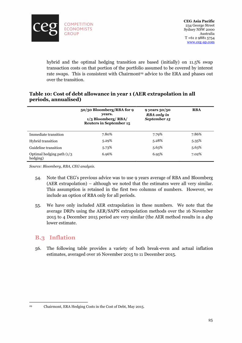
53. Table 10 below provides estimates of the cost of debt for each transition

methodology in the first year of the transition. The first nine averaging periods are

calendar years 2006 to 2014.28 The final averaging period is the 15 days to 4

December 2015. All estimates are based on AER extrapolation. In addition, the

27 Our reasoning is explained in more detail in recent reports for AGN, SAPN and United Energy. For

example: CEG, Measuring expected inflation for the PTRM, a report for United Energy, January 2016.

28 The first averaging period is from 1 January 2006 to 31 December 2006, while the ninth averaging

period is from 1 January 2014 to 31 December 2014.

CEG Asia Pacific

234 George Street Sydney NSW 2000

Australia T +61 2 9881 5754

www.ceg-ap.com

25

hybrid and the optimal hedging transition are based (initially) on 11.5% swap

transaction costs on that portion of the portfolio assumed to be covered by interest

rate swaps. This is consistent with Chairmont29 advice to the ERA and phases out

over the transition.

Table 10: Cost of debt allowance in year 1 (AER extrapolation in all periods, annualised)

50/50 Bloomberg/RBA for 9 years.

1/3 Bloomberg/ RBA/ Reuters in September 15

9 years 50/50

RBA only in September 15

RBA

Immediate transition 7.80% 7.79% 7.86%

Hybrid transition 5.29% 5.28% 5.35%

Guideline transition 5.73% 5.63% 5.63%

Optimal hedging path (1/3 hedging)

6.96% 6.95% 7.02%

Source: Bloomberg, RBA, CEG analysis.

54. Note that CEG’s previous advice was to use 9 years average of RBA and Bloomberg

(AER extrapolation) – although we noted that the estimates were all very similar.

This assumption is retained in the first two columns of numbers. However, we

include an option of RBA only for all periods.

55. We have only included AER extrapolation in these numbers. We note that the

average DRPs using the AER/SAPN extrapolation methods over the 16 November

2015 to 4 December 2015 period are very similar (the AER method results in a 4bp

lower estimate.

B.3 Inflation

56. The following table provides a variety of both break-even and actual inflation

estimates, averaged over 16 November 2015 to 11 December 2015.

29 Chairmont, ERA Hedging Costs in the Cost of Debt, May 2015.

CEG Asia Pacific

234 George Street Sydney NSW 2000

Australia T +61 2 9881 5754

www.ceg-ap.com

26

Table 11: Break-even (and actual) inflation estimates (averaged over 16 November 2015 to 11 December 2015)

Estimate Value Estimate Value

10 year 2.25%

5 year 2.01%

4 year 1.94%

Actual Jun 14 to Jun 15 (annualised)

1.51% Weighted average of 10 year and 5 year break

even (60% of 5-year and 40% of 10-year) 2.11%

80% of 4 year forecast and 20% of 1 year actual

1.85% Weighted average of 10 year and 5 year (where 5

year estimate is 25% actual and 75% forecast) 2.01%

Source: Bloomberg, RBA, ABS, CEG analysis. Note that we have simply updated the values in this table.

However, more up-to-date actual inflation will be available at the time of the AER’s final decision and, in

relation to the cost of debt component of the RAB, the AER should have regard to that as well as to forecast

inflation at that time.

57. The following estimates are appropriate in each circumstance:

10 year break even (2.25%) – if all that is being challenged is the source of

forecast estimate;

Weighted average of 10 and 5 year break even (2.12%) – if it is accepted that

debt costs are nominal costs and, therefore, in order to deliver appropriate

compensation the PTRM should adopt the same term for the inflation forecast

as the regulatory period;

Weighted average of 10 and a mix of actual and forecast inflation over 5 years

from June 2014 (2.01%) – as above plus recognition that the 5 year term should

cover the same period as will be covered in the next RFM model (which we

understand will be from June 2014 to June 2019).

58. We consider that the last of these options is the economically correct one.

B.4 16 Nov 2015 – 4 Dec 2015 swap values

59. The following table provides the swap values for the 15 business days from 16

November 2015 to 4 December 2015, as used in our calculations of the cost of debt.

CEG Asia Pacific

234 George Street Sydney NSW 2000

Australia T +61 2 9881 5754

www.ceg-ap.com

27

Table 12: Daily swap rates over 16 November 2015 to 4 December 2015 by maturity (semi-annual)

1 2 3 4 5 6 7 8 9 10

16/11/2015 2.293 2.282 2.343 2.4415 2.5738 2.6964 2.7966 2.8979 2.9813 3.0555

17/11/2015 2.298 2.283 2.337 2.4313 2.5538 2.675 2.785 2.885 2.96 3.0325

18/11/2015 2.3 2.29 2.35 2.4438 2.5799 2.6925 2.7988 2.8955 2.9863 3.0438

19/11/2015 2.299 2.287 2.356 2.4438 2.5706 2.6681 2.7881 2.8869 2.9656 3.0225

20/11/2015 2.3025 2.2925 2.37 2.4613 2.5838 2.71 2.8144 2.905 2.98 3.0563

23/11/2015 2.32 2.315 2.38 2.4544 2.5769 2.695 2.8025 2.8938 2.97 3.04

24/11/2015 2.321 2.313 2.39 2.4688 2.6011 2.711 2.8169 2.9106 2.9938 3.0563

25/11/2015 2.32 2.311 2.3775 2.4463 2.5631 2.655 2.7736 2.8588 2.9418 3.0138

26/11/2015 2.3 2.276 2.333 2.3963 2.5125 2.6 2.7156 2.7925 2.8825 2.9498

27/11/2015 2.33 2.297 2.368 2.4588 2.5613 2.665 2.7613 2.85 2.9275 2.9925

30/11/2015 2.32 2.302 2.355 2.4338 2.545 2.6413 2.7444 2.8306 2.905 2.9725

1/12/2015 2.316 2.298 2.358 2.4438 2.5313 2.6313 2.7238 2.805 2.8825 2.9475

2/12/2015 2.346 2.332 2.381 2.4544 2.5475 2.6513 2.7506 2.8381 2.915 2.9813

3/12/2015 2.3425 2.354 2.424 2.51 2.6164 2.7375 2.8413 2.9363 3.0188 3.0855

4/12/2015 2.358 2.376 2.426 2.4988 2.6138 2.7156 2.8238 2.9129 2.9954 3.065

Source: Bloomberg

B.5 Historical swap and DRP values

60. The following table provides the historical DRP values used in our calculations.

Table 13: Historical DRPs (measured to swap values, semi-annual)

Calendar year (unless otherwise

stated)

10 year swap rates

RBA (AER extrapolation)

Bloomberg (AER extrapolation)

Reuters*

2006 6.077 0.707 0.579 2007 6.639 1.067 0.816 2008 6.659 3.583 2.362 2009 5.591 4.519 3.373 2010 5.872 2.107 3.454 2011 5.505 2.370 3.286 2012 4.165 3.151 3.017 2013 4.238 3.018 2.665 2014 4.011 2.238 1.879

2015 (16 Nov – 4 Dec) 3.021 2.533 2.520 2.8385

Source: Bloomberg, AER, RBA, Reuters and CEG analysis; *Reuters DRP calculated using Bloomberg swap

rates. If Reuters spreads are used, the resulting average DRP would be 2.8313%.

CEG Asia Pacific

234 George Street Sydney NSW 2000

Australia T +61 2 9881 5754

www.ceg-ap.com

28

Appendix C Terms of reference

1 Background

Jemena Electricity Networks (JEN) is an electricity distribution network service provider in Victoria.

JEN supplies electricity to approximately 300,000 homes and businesses through its 10,285

kilometres of distribution system. JEN’s electricity distribution system services 950 square kilometres

of northwest greater Melbourne. JEN’s electricity network is maintained by infrastructure management

and services company, Jemena Asset Management (JAM).

JEN submitted its initial regulatory proposal with supporting information for the consideration of the

Australian Energy Regulator (AER) on 30 April 2015. This proposal covers the period 2016-2020

(calendar years). The AER published its preliminary decision on 29 October 2015. JEN made a

submission on revocation and substitution of the preliminary decision to the AER on 6 January 2016.

As with all of its economic regulatory functions and powers, when making the distribution

determination to apply to JEN under the National Electricity Rules and National Electricity Law, the

AER is required to do so in a manner that will or is likely to contribute to the achievement of the

National Electricity Objective, which is:

to promote efficient investment in, and efficient operation and use of, electricity services for

the long term interests of consumers of electricity with respect to:

(a) price, quality, safety, reliability and security of supply of electricity; and

(b) the reliability, safety and security of the national electricity system.

Where the AER is making a distribution determination and there are two or more possible decisions

that will or are likely to contribute to the achievement of the National Electricity Objective, the AER is

required to make the decision that the AER is satisfied will or is likely to contribute to the achievement

of the National Electricity Objective to the greatest degree.

The AER must also take into account the revenue and pricing principles in section 7A of the National

Electricity Law when exercising its discretion in making those parts of a distribution determination

relating to direct control network services. The revenue and pricing principles include the following:

A regulated network service provider should be provided with a reasonable opportunity to

recover at least the efficient costs the operator incurs in:

(a) providing direct control network services; and

(b) complying with a regulatory obligation or requirement or making a regulatory payment.

Some of the key rules governing the making of a distribution determination are set out below.

CEG Asia Pacific

234 George Street Sydney NSW 2000

Australia T +61 2 9881 5754

www.ceg-ap.com

29

Clause 6.4.3(a) of the National Electricity Rules provides that revenue for a regulated service provider

is to be calculated adopting a “building block approach”. It provides:

The annual revenue requirement for a Distribution Network Service Provider for each

regulatory year of a regulatory control period must be determined using a building block

approach, under which the building blocks are:

(1) indexation of the regulatory asset base – see paragraph (b)(1);

(2) a return on capital for that year – see paragraph (b)(2);

(3) the depreciation for that year – see paragraph (b)(3);

(4) the estimated cost of corporate income tax of the Distribution Network Service Provider for

that year – see paragraph (b)(4);

(5) the revenue increments or decrements (if any) for that year arising from the application of

any efficiency benefit sharing scheme, capital expenditure sharing scheme, service target

performance incentive scheme, demand management and embedded generation

connection incentive scheme or small-scale incentive scheme – see subparagraph (b)(5);

(6) the other revenue increments or decrements (if any) for that year arising from the

application of a control mechanism in the previous regulatory control period – see

paragraph (b)(6);

(6A) the revenue decrements (if any) for that year arising from the use of assets that

provide standard control services to provide certain other services – see subparagraph

(b)(6A); and

(7) the forecast operating expenditure for that year – see paragraph (b)(7).

Clause 6.5.2 of the National Electricity Rules, relating to the allowed rate of return, states:

Calculation of return on capital

(a) The return on capital for each regulatory year must be calculated by applying a rate of

return for the relevant Distribution Network Service Provider for that regulatory year

that is determined in accordance with this clause 6.5.2 (the allowed rate of return) to

the value of the regulatory asset base for the relevant distribution system as at the

beginning of that regulatory year (as established in accordance with clause 6.5.1 and

schedule 6.2).

Allowed rate of return

(b) The allowed rate of return is to be determined such that it achieves the allowed rate of

return objective.

CEG Asia Pacific

234 George Street Sydney NSW 2000

Australia T +61 2 9881 5754

www.ceg-ap.com

30

(c) The allowed rate of return objective is that the rate of return for a Distribution Network

Service Provider is to be commensurate with the efficient financing costs of a

benchmark efficient entity with a similar degree of risk as that which applies to the

Distribution Network Service Provider in respect of the provision of standard control

services (the allowed rate of return objective).

(d) Subject to paragraph (b), the allowed rate of return for a regulatory year must be:

(1) a weighted average of the return on equity for the regulatory control period in

which that regulatory year occurs (as estimated under paragraph (f)) and the

return on debt for that regulatory year (as estimated under paragraph (h));

and

(2) determined on a nominal vanilla basis that is consistent with the estimate of

the value of imputation credits referred to in clause 6.5.3.

(e) In determining the allowed rate of return, regard must be had to:

(1) relevant estimation methods, financial models, market data and other

evidence;

(2) the desirability of using an approach that leads to the consistent application of

any estimates of financial parameters that are relevant to the estimates of,

and that are common to, the return on equity and the return on debt; and

(3) any interrelationships between estimates of financial parameters that are

relevant to the estimates of the return on equity and the return on debt.

Return on equity

(f) The return on equity for a regulatory control period must be estimated such that it

contributes to the achievement of the allowed rate of return objective.

(g) In estimating the return on equity under paragraph (f), regard must be had to the

prevailing conditions in the market for equity funds.

Return on debt

(h) The return on debt for a regulatory year must be estimated such that it contributes to

the achievement of the allowed rate of return objective.

(i) The return on debt may be estimated using a methodology which results in either:

(1) the return on debt for each regulatory year in the regulatory control period

being the same; or

CEG Asia Pacific

234 George Street Sydney NSW 2000

Australia T +61 2 9881 5754

www.ceg-ap.com

31

(2) the return on debt (and consequently the allowed rate of return) being, or

potentially being, different for different regulatory years in the regulatory

control period.

(j) Subject to paragraph (h), the methodology adopted to estimate the return on debt

may, without limitation, be designed to result in the return on debt reflecting:

(1) the return that would be required by debt investors in a benchmark efficient

entity if it raised debt at the time or shortly before the making of the

distribution determination for the regulatory control period;

(2) the average return that would have been required by debt investors in a

benchmark efficient entity if it raised debt over an historical period prior to the

commencement of a regulatory year in the regulatory control period; or

(3) some combination of the returns referred to in subparagraphs (1) and (2).

(k) In estimating the return on debt under paragraph (h), regard must be had to the

following factors:

(1) the desirability of minimising any difference between the return on debt and

the return on debt of a benchmark efficient entity referred to in the allowed

rate of return objective;

(2) the interrelationship between the return on equity and the return on debt;

(3) the incentives that the return on debt may provide in relation to capital

expenditure over the regulatory control period, including as to the timing of

any capital expenditure; and

(4) any impacts (including in relation to the costs of servicing debt across

regulatory control periods) on a benchmark efficient entity referred to in the

allowed rate of return objective that could arise as a result of changing the

methodology that is used to estimate the return on debt from one regulatory

control period to the next.

(l) If the return on debt is to be estimated using a methodology of the type referred to in

paragraph (i)(2) then a resulting change to the Distribution Network Service Provider's

annual revenue requirement must be effected through the automatic application of a

formula that is specified in the distribution determination.”

[Subclauses (m)–(q) omitted].

In its initial proposal and its submission on revocation and substitution of the preliminary decision,

JEN submitted expert reports from CEG, SFG and UBS (the Earlier Reports) on the appropriate

CEG Asia Pacific

234 George Street Sydney NSW 2000

Australia T +61 2 9881 5754

www.ceg-ap.com

32

approach to be adopted in estimating the return on debt for the benchmark efficient entity.30 JEN’s

submission also noted that:31

230. JEN will provide the AER with updated estimates of the prevailing return on debt and the

year one return on debt once the data for JEN’s actual averaging period has been analysed.

231. In estimating the prevailing return on debt for the actual averaging period, JEN will use the

data source selection method set out in section 2.5.1 [of Attachment 6-1 to JEN’s

submission], with some modification. For the purposes of estimating the prevailing return on

debt for the first year, JEN will seek the best estimate of the prevailing return on debt,

regardless of whether the available data sources diverge by more than 60 basis points. JEN

intends to seek expert advice as to the best estimate for the actual averaging period, with

this advice to draw on the results the data source selection method set out in section 2.5.1

above (not constrained by the 60 basis point divergence threshold) and any other factors the

expert considers relevant for that period.

232. For the first year estimate, we do not consider it necessary to impose the divergence

threshold or to adopt a simple average of available data sources as the starting point, since

the best performing data source can be identified as part of the AER’s broader

consideration of return on debt issues in its distribution determination (i.e. the assessment

for year one is not subject to any constraints that may be seen to apply to the annual update

process).

In this context, JEN seeks a report from CEG, as a suitable qualified independent expert (Expert), to

update the return on debt for JEN’s actual averaging period (being 16 November 2015 to 4 December

2015).

2 Scope of Work

The Expert will provide an opinion report that:

1. Determine the best estimate of the prevailing return on debt for JEN’s averaging period (16

November to 4 December), considering:

30 CEG, Critique of the AER’s JGN draft decision on the cost of debt, April 2015; SFG, Return on debt transition

arrangements under the NGR and NER, February 2015; UBS, Transaction Costs and the AER Return

on Debt Draft Determination, March 2015; CEG, Critique of AER analysis on New Issue Premium,

December 2015; CEG, Memorandum – September 2015 cost of debt and inflation forecasts, 5 January

2016; CEG, Critique of the AER’s approach to transition, January 2016; and CEG, Criteria for assessing

fair value curves, January 2016.

31 JEN, Submission on revocation and substitution of the preliminary decision, Attachment 6-1, p 36.

CEG Asia Pacific

234 George Street Sydney NSW 2000

Australia T +61 2 9881 5754

www.ceg-ap.com

33

(a) Relevant data sources, including from the Reserve Bank of Australia (RBA), Bloomberg and Reuters;

(b) The method or methods for testing the fit of various data sources to traded bond data previously recommended by the Expert;

(c) Any other factors that the Expert considers relevant.

2. Using the estimate from (1), determine the best estimate of the return on debt for the first year of

the following transitions to the trailing average return on debt:

(a) An immediate transition;

(b) A hybrid transition, assuming that 100% of the base rate was hedged;

(c) A hybrid transition, assuming that only one third (1/3) of the base rate was hedged; and

(d) The transition set out in the AER’s rate of return guideline.

In preparing the report the Expert will:

A. use a simple average of Bloomberg and RBA data for the first nine (9) years of any historical

averages;

B. assume a 10 year term and a BBB to BBB+ credit rating; and

C. use robust methods and data in producing any statistical estimates.

3 Information to be Considered

The Expert is also expected to consider the following information:

• such information that, in Expert’s opinion, should be taken into account to address the questions

outlined above;

• relevant literature on estimating the return on debt;

• the AER’s Rate of Return Guideline, including explanatory statements and supporting expert

material;

• material submitted to the AER as part of its consultation on the Rate of Return Guidelines; and

• previous decisions of the AER, other relevant regulators and the Australian Competition Tribunal

on the return on debt and any supporting expert material, including the recent final decisions for

Jemena Gas Networks and electricity networks in ACT, NSW, Queensland, South Australia and

Tasmania.

CEG Asia Pacific

234 George Street Sydney NSW 2000

Australia T +61 2 9881 5754

www.ceg-ap.com

34

4 Deliverables

At the completion of its review the Expert will provide an independent expert report which:

• is of a professional standard capable of being submitted to the AER;

• is prepared in accordance with the Federal Court Practice Note on Expert Witnesses in

Proceedings in the Federal Court of Australia (CM 7) set out in Attachment 1, and includes an

acknowledgement that the Expert has read the guidelines 32;

• contains a section summarising the Expert’s experience and qualifications, and attaches the

Expert’s curriculum vitae (preferably in a schedule or annexure);

• identifies any person and their qualifications, who assists the Expert in preparing the report or in

carrying out any research or test for the purposes of the report;

• summarises JEN’s instructions and attaches these term of reference;

• includes an executive summary which highlights key aspects of the Expert’s work and

conclusions; and

• (without limiting the points above) carefully sets out the facts that the Expert has assumed in

putting together his or her report, as well as identifying any other assumptions made, and the

basis for those assumptions.

The Expert’s report will include the findings for each of the three parts defined in the scope of works

(Section 2).

5 Timetable

The Expert will deliver the final report to Jemena Regulation by 5 February 2016.

6 Terms of Engagement

The terms on which the Expert will be engaged to provide the requested advice shall be:

as provided in accordance with the Jemena Regulatory Consultancy Services Panel

arrangements applicable to the Expert.

32 Available at: http://www.federalcourt.gov.au/law-and-practice/practice-documents/practice-notes/cm7.

CEG Asia Pacific

234 George Street Sydney NSW 2000

Australia T +61 2 9881 5754

www.ceg-ap.com

35

ATTACHMENT 1: FEDERAL COURT PRACTICE NOTE

Practice Note CM 7

EXPERT WITNESSES IN PROCEEDINGS IN THE FEDERAL COURT OF AUSTRALIA

Commencement

1. This Practice Note commences on 4 June 2013.

Introduction

2. Rule 23.12 of the Federal Court Rules 2011 requires a party to give a copy of the following guidelines to any witness they propose to retain for the purpose of preparing a report or giving evidence in a proceeding as to an opinion held by the witness that is wholly or substantially based on the specialised knowledge of the witness (see Part 3.3 - Opinion of the Evidence Act 1995 (Cth)).

3. The guidelines are not intended to address all aspects of an expert witness’s duties, but are intended to facilitate the admission of opinion evidence33, and to assist experts to understand in general terms what the Court expects of them. Additionally, it is hoped that the guidelines will assist individual expert witnesses to avoid the criticism that is sometimes made (whether rightly or wrongly) that expert witnesses lack objectivity, or have coloured their evidence in favour of the party calling them.

Guidelines

1. General Duty to the Court34 1.1 An expert witness has an overriding duty to assist the Court on matters relevant to the expert’s

area of expertise.

1.2 An expert witness is not an advocate for a party even when giving testimony that is necessarily evaluative rather than inferential.

1.3 An expert witness’s paramount duty is to the Court and not to the person retaining the expert.

2. The Form of the Expert’s Report35 2.1 An expert’s written report must comply with Rule 23.13 and therefore must

(a) be signed by the expert who prepared the report; and

(b) contain an acknowledgement at the beginning of the report that the expert has read,

understood and complied with the Practice Note; and

(c) contain particulars of the training, study or experience by which the expert has

acquired specialised knowledge; and

33 As to the distinction between expert opinion evidence and expert assistance see Evans Deakin Pty Ltd v

Sebel Furniture Ltd [2003] FCA 171 per Allsop J at [676].

34 The “Ikarian Reefer” (1993) 20 FSR 563 at 565-566.

35 Rule 23.13.

CEG Asia Pacific

234 George Street Sydney NSW 2000

Australia T +61 2 9881 5754

www.ceg-ap.com

36

(d) identify the questions that the expert was asked to address; and

(e) set out separately each of the factual findings or assumptions on which the expert’s

opinion is based; and

(f) set out separately from the factual findings or assumptions each of the expert’s

opinions; and

(g) set out the reasons for each of the expert’s opinions; and

(ga) contain an acknowledgment that the expert’s opinions are based wholly or

substantially on the specialised knowledge mentioned in paragraph (c) above36; and

(h) comply with the Practice Note.

2.2 At the end of the report the expert should declare that “[the expert] has made all the inquiries that [the expert] believes are desirable and appropriate and that no matters of significance that [the expert] regards as relevant have, to [the expert’s] knowledge, been withheld from the Court.”

2.3 There should be included in or attached to the report the documents and other materials that the expert has been instructed to consider.

2.4 If, after exchange of reports or at any other stage, an expert witness changes the expert’s opinion, having read another expert’s report or for any other reason, the change should be communicated as soon as practicable (through the party’s lawyers) to each party to whom the expert witness’s report has been provided and, when appropriate, to the Court37.

2.5 If an expert’s opinion is not fully researched because the expert considers that insufficient data are available, or for any other reason, this must be stated with an indication that the opinion is no more than a provisional one. Where an expert witness who has prepared a report believes that it may be incomplete or inaccurate without some qualification, that qualification must be stated in the report.

2.6 The expert should make it clear if a particular question or issue falls outside the relevant field of expertise.

2.7 Where an expert’s report refers to photographs, plans, calculations, analyses, measurements, survey reports or other extrinsic matter, these must be provided to the opposite party at the same time as the exchange of reports38.

3. Experts’ Conference

3.1 If experts retained by the parties meet at the direction of the Court, it would be improper for an expert to be given, or to accept, instructions not to reach agreement. If, at a meeting directed by the Court, the experts cannot reach agreement about matters of expert opinion, they should specify their reasons for being unable to do so.

J L B ALLSOP

Chief Justice

4 June 2013

36 See also Dasreef Pty Limited v Nawaf Hawchar [2011] HCA 21.

37 The “Ikarian Reefer” [1993] 20 FSR 563 at 565

38 The “Ikarian Reefer” [1993] 20 FSR 563 at 565-566. See also Ormrod “Scientific Evidence in Court” [1968]

Crim LR 240

CEG Asia Pacific

234 George Street Sydney NSW 2000

Australia T +61 2 9881 5754

www.ceg-ap.com

37

Appendix D Curriculum vitae

Curriculum Vitae

Dr Tom Hird / Director

Contact Details

T / +61 (3) 9095 7570

M / +61 422 720 929

E / tom.hird@ceg-ap.com

Key Practice Areas

Tom Hird is a founding Director of CEG’s Australian operations. In the eight years since its inception

CEG has been recognised by Global Competition Review (GCR) as one of the top 20 worldwide

economics consultancies with focus on competition law. Tom has a Ph.D. in Economics from Monash

University. Tom is also named by GCR in its list of top individual competition economists.

Tom’s clients include private businesses and government agencies.

In terms of geographical coverage, Tom's clients have included businesses and government agencies

in Australia, Japan, Korea, the UK, France, Belgium, Poland, Germany, the Netherlands, New

Zealand, Macau, Singapore and the Philippines. Selected assignments are set out below.

Selected Recent Projects Advice on the impact of information exchange on competition.

Retained by Sainsbury’s to advise on the present value of damages to be claimed from

MasterCard in relation to excessive interchange fees.

Advice on optimal hedging ratio for a number of regulated businesses.

Advice to NSW, Victorian and ACT electricity and gas distribution businesses to estimate the

cost of capital for these businesses.

Expert report for the AEMC on market power and barriers to entry in the markets for electricity

generation within the Australian National Electricity Market.

Expert evidence for Chorus (the New Zealand incumbent fixed line telecommunications access

supplier) on the design of the regulatory regime to be applied to its new fibre broadband

investments.

CEG Asia Pacific

234 George Street Sydney NSW 2000

Australia T +61 2 9881 5754

www.ceg-ap.com

38

Advice to Vector in relation to an acquisition of another New Zealand electricity metering

business.

Advice to Vector in relation to a NZ Commerce Commission inquiry considering extending

regulation to gas metering.

Expert advice to the ACCC in relation to the competition implications of an acquisition of equity

in Channel 10 by parties with an interest in Foxtel (a potential competitor of Channel 10).

Adviser to the arbiter on a commercial arbitration in the iron ore sector.

Expert advice to the ACCC in relation to the merger of petrol station outlets in Adelaide.

Expert advice to the Australian Government Solicitor in relation to the economic impact of

plain paper packaging regulations for cigarettes and other tobacco products.

Expert evidence on the cost of capital to the New Zealand Airports Association and the New

Zealand Energy Networks Association.

Expert evidence to Everything Everywhere in relation to the cost of UK mobile operators -

including oral testimony before the UK Commerce Commission.

Expert evidence to the Australian Energy Networks Association on a range of issues in relation

to estimating the cost of capital for regulated energy infrastructure businesses.

Expert evidence to T-Mobile (Deutsche Telekom) on the cost of capital for mobile operators

operating in Western Europe.

Expert evidence, prepared for Japanese steel mills, submitted to the numerous regulators

(including the EC, JFTC and ACCC) on the competition impact of the then proposed iron ore

joint venture between BHPB and Rio Tinto. CEG, along with other parties retained by the

Japanese steel mills, received the GCR award for M&A Transaction of the Year -- Asia-Pacific,

Middle East and Africa.

Advising Vivendi on the correct cost of capital to use in a discounted cash flow analysis in a

damages case being brought by Deutsche Telekom.

Expert evidence to Vector on appeal of the New Zealand Commerce Commission decision on

the cost of capital.

Expert evidence in relation to the cost of capital for Victorian gas transport businesses.

Expert evidence to the Australian Competition Tribunal on the cost of debt for Jemena

Electricity Networks.

Advice to Integral Energy on optimal capital structure.

Expert evidence NSW, ACT and Tasmanian electricity transmission and distribution businesses

on the cost of capital generally and how to estimate it in the light of the global financial crisis.

Expert evidence in relation to the appeal by the above businesses of the Australian Energy

Regulator (AER) determination.

Expert testimony to the Federal Court of Australia on alleged errors made by the Australian

Competition and Consumer Commission (ACCC) in estimating the cost of capital for Telstra.

Expert evidence the AER on the cost capital issues in relation to the RBP pipeline access

arrangement.

Expert evidence to the ENA on the relative merits of CBASpectrum and Bloomberg's

methodology for estimating the debt margin for long dated low rated corporate bonds.

Expert evidence the Australian Competition and Consumer Commission, Australia on the

correct discount rate to use when valuing future expenditure streams on gas pipelines.