TECHNOLOGY

BEHIND

ELECT

A

COMPUTER PROGRAM

ON

CABLES & OVERHEAD LINES

WITH SPECIFIC AND WIDE COVERGAE ON ENERGY AUDIT

&

SAG-TENSION IN OVERHEAD LINES

December 2005

By:

Mohammed Zahoor Ali

i

C O N T E N T S

Sl. no.

D E S C R I P T I O N Page no.

1 Preface

1

2 Introduction

1A

3 About Energy Audit

2

4 Distribution System of Electrical Energy

3

Voltage drop and percentage regulation in overhead lines.

3

(i) When sending end voltage is known 3

5

(ii) When receiving end voltage is known

6

Selection of overhead line conductors (ACSR/ AAAC).

10

(i) RMS current 10 (ii) Form factor and Load factor 10

(iii) Establishment of cost constant of conductor 'P' 12 (iv) Cost estimate of 33 kV overhead line 12 (v) Cost estimate of 11 kV overhead line 12

(vi) Cost estimate of 6.6 kV overhead line 13 (vii) Cost estimate of 3.3 kV overhead line 13

(viii) Cost estimate of 415 V overhead line 13 (ix) Cost of conductors as on Sept. 2003 in rupees 14 (x) Energy loss during transmission 15

6

(xi) Voltage regulation of OHL

16

Calculations for MW-km of overhead lines (ACSR/ AAAC) 17 (i) Weight of conductor 17

(ii) Sag of overhead line 17 (iii) Spacing between conductors 18 (iv) Resistance of conductor 18

7

(v) Maximum active and reactive power through overhead lines

18

Cable selection

22

(i) Selection based on RMS current 22

8

(ii) Selection based on Voltage regulation 22

ii

(iii) Effect of temperature on resistance, inductance and capacitance

23

(iv) Voltage regulation 23 (v) Selection based on Fault current 23

(vi) Losses in cables Conductor I2r loss Dielectric loss Sheath loss

24 24 25 26

Resistance, Inductance, Capacitance, Sag and Conductor spacing calculations of overhead lines with ACSR/ AAAC conductors

26 (i) Sag of overhead lines 26

(ii) Spacing between conductors and equivalent spacing 27 (iii) Inductance of 3 phase overhead line 28 (iv) Capacitance of 3 phase overhead line 28

9

(v) Resistance of overhead line

29

Most economical power factor of a system

29

(i) Definitions of Most Economical pf and Most Suitable/ Desirable power factor

30

10

(ii) Derivations for Most Suitable and Most Economical power factors

30

11 Corona loss

33

12 Voltage regulation and drop in Cables

34

Sag and Tension in overhead lines

36

(a) Effective weight of conductor 36

13

(b) Factor of safety for conductors

38

Sample Calculations

39

(a) Voltage regulation & drop when sending end voltage is known

39

(b) Voltage regulation & drop when receiving end voltage is known with results generated for (a) & (b)

41

(c) Most Economical Conductor Selection 48 (d) Cable Selection with results generated 53

14

(e) Sag & Tension in overhead lines (Refer ‘Show Calculations’ in program menu of ELECT )

-

iii

TABLES

1 Copper cables properties

59

2 Aluminium cables properties

59

3 Default data of ACSR conductors

60

4 Calculated data of ACSR conductors

60

5 Default data of AAAC conductors

61

6 Calculated data of AAAC conductors

61

7 User data of AAC conductor (Sample)

62

8 User data of ACSR conductor (Sample)

62

9 Physical constants used to calculate ACSR data

63

15

10 Physical constants used to calculate AAAC data

63

COSTING OF 3-PHASE POWER CABLES

64

A Table showing cost trends of different category of 3-phase power cables

65

B Cost difference between Copper and Aluminium conductor cables

66

C Empirical Formulae for costing of 3-Core Power Cables

67

16

D Power Cables of 3½ and 4-Cores Power Cables

68

17 COSTING OF OVERHEAD TRANS. LINES

69

A Conductor cost index as on reference date 69

B Overhead Line Pole/ Tower structures and basis of costing 69

C Different grade Insulators and basis of costing 71

iv

D Earth conductor and Earthing 73

E Ruling Span of overhead line 73

F Empirical Formulae considering all factors 74

18 SAMPLE GENERATED REPORTS

75

A Energy Audit of OHL 75

B Results of Voltage Regulation 77

C Results of Most Economical Conductor Selection 78

D Results of Sag & Tension Calculations as per IS 79

E Results of Verification of Energy Bill Calculations 84

F Transformer Impedance Calculations 87

G Results of Transformer Impedance 90

H Results of Cable Selection by different methods 91

J Results of voltage regulation and drop in cables 93

K Results of Item-wise details of overhead line costing 94

L Results of Power Balance & Capacitor Bank selection 95

M Results of Sag and Tension program execution 97

N Graphical results of Bill Analysis and Most Economical Conductor Selection 98

19 PROPERTIES OF OVERHEAD LINE CONDUCTORS

100

A Conductor Radius, Equivalent Al area, nominal equivalent cu area 101

B Current density, empirical formulae, R, Xl, Xc, Weight, Tensile strength of conductors 102

C Rule 54 & 55 of Indian Electricity Rule 1956 for supply voltage regulation 105

0

PREFACE

Cables and overhead lines are integral part of any Electrical system or network. Larger the network, greater is the complexity. The ELECT computer program has been prepared to solve the complex conditions by feeding minimum possible information. This part of the program deals with Overhead Lines, Cables and Transformers. Although, each of these has a vast technology, it has been tried to arrive at more accurate results by using more practicable solutions. The latest version of this Software has included the following:

1. Cost estimate of Overhead Lines 2. Energy Bill Analysis with graphical display 3. Cost estimate of different type and grade of Power Cables. 4. Back-up calculations of Sag/Tension, Energy Bill verification and

Percentage Impedance of Transformers. 5. Technology behind Elect in PDF format

This ELECT software may be divided in the following three categories: 1. Software part

2. User’s Manual part 3. Technology part Software part is the main computer program prepared in high-level languages and is very much user friendly. However, it is essential to understand the aims and objectives of this software before use. User’s Manual is in the form of a booklet. This manual is also provided in PDF Format, along-with this software, so that any number of copies can be reproduced if necessary. Technology part as mentioned above at (5) is now being supplied with this software in PDF format. Readers and Users may like to send their healthy suggestions, if any, for improvement of this program. They will be cordially accepted with thanks and shall be tried to incorporate in its future versions. Readers of this book and users of the ELECT software may feel free to email their comments directly to the authors. Bhubaneswar Authors 15th January 2005 sofexindia@yahoo.com

1

INTRODUCTION

Energy conservation can be considered as an alternate source of energy. The cost of supplying incremental energy is far less if it is made up by implementing energy conservation measures as against the investment required to create equivalent resources. The expert committee, constituted by Government of India, has suggested all large and medium sized industries: 1. To carry out detailed energy audits. 2. To improve the efficiency of utilisation. 3. To appoint energy managers as a mandatory measure. 4. To use energy efficient equipment. 5. To review and identify the R&D efforts required to reduce energy

consumption for every major industrial process. 6. To organise formal training courses for developing energy conservation

expertise. 7. To form a system of government recognition and awards for honouring

individuals and organisations for outstanding performances in energy conservation.

The above is a list of few extracted measures of the expert committee on energy, which speaks of itself about the importance of energy conservation. In view of the experts committee’s recommendations, the importance of the ELECT software has increased. Moreover, the ELECT Software Version-7 has included the following topics to make it more suitable for practical utilisation: 1. Conductor cost index (area index) has been revised and made upto-date

and is now suitable for use in any country/ currency. 2. Overhead Line costing with different possible specifications. 3. Default data set has been included as per Indian standards. 4. Voltage regulation/ drop, losses etc. now can be found for single as well

bundled conductors/cables with same or unequal sizes. 5. Graphical illustration of the most economical conductor selection. 6. Complete energy audit reports of overhead lines at fingertips. 7. Attractive get up and user-friendly presentation. 8. A complete and exhaustive programme on Sag and Tension of overhead

lines with facility to view each and every calculation. 9. Complete technology behind the ELECT software in pdf format. 10. A complete & separate program on Cable Properties, Cable Selection and

Regulation/ Voltage Drop/ Losses in single or bundled cables. 11. Cable Selection, load analysis & costing 12. Transformer Selection, pf improvement, power balance etc.

2

ABOUT ENERGY AUDIT In a developing country, like ours, the demand of energy is continuously growing at a higher

rate than normal, widening the gap between demand and supply. Bridging this gap is a costly affair.

For most of the industries, the share of energy cost in the total production cost is quite

significant. Reduction of energy cost can improve profit levels in such cases. The reduction can be achieved by improving the efficiency of industrial operations and equipment.

Energy audits play an important role in identifying energy conservation opportunities in the

industrial sector. While they do not provide the final answer to the problem, they do help to identify the existing potential for energy conservation, and induces the companies to concentrate their efforts in this area in a focussed manner.

The cost of domestic as well as commercial energy is very high compared to many other

countries of the world. With the fact that conservation of energy will grow at a robust pace with the increased level of economic activity, the cost of energy production and consumption would become much higher in future.

The industries sector alone consumes about 50% of the total commercial energy, while it

contributes only about 25% of the country’s GDP. Several efforts at analysing the potentials of energy savings in the industrial sector indicate a

range of 20% - 25% reduction without significant investments. For any industrial unit, the first step in adopting a plan for improvement of energy efficiency

is to carry out an energy audit. Energy audit provides a quantitative and technical base for assessing how different forms of energy are being used and for quantifying energy used according to discrete functions. They are important tools for identifying the potentials for improvements in the energy efficiencies, and indicate direction towards on which energy management efforts should be concentrated.

ELECTRICAL ENERGY This book has covered the technology used behind the electrical energy audit software

ELECT. The ELECT software deals with the engineering of overhead transmission lines and cables, with specific stress on energy audit aspects. The purpose of the ELECT software is to provide a technical platform for finding suitable, most economical, technically feasible, standard and easily available conductor or cable for an electrical system with due consideration of the system stability and other relevant technical requirements. The ELECT software is very much useful for in-depth audit of energy transmission and distribution through an overhead line or cable.

Energy audit of a system can be categorised as under:

1. Transmission & Distribution System e.g. Overhead lines, cables, transformers etc. 2. Mechanical System performing a job e.g. motors, pumps, transport etc.

A number of losses/ wastages occur between the point of generation of electrical energy and

its actual consumption in performing a job. The purpose of energy audit is to check for the losses and wastages of electrical energy flow system. This boo has restricted discussion on Transmission and Distribution network only.

3

DISTRIBUTION SYSTEMS OF ELECTRICAL ENERGY Distribution network for the electrical energy is normally done through the following

two systems: 1. Overhead transmission line network system 2. Cable network system

In overhead line system, two types of situation may arise. Firstly, when the ‘Sending

End voltage is known’ and secondly, when the ‘Receiving end voltage’ is known. Both these aspects of the overhead lines are discussed hereunder.

However, it is to be noted here that the effect of line capacitance has only been taken

in the second case, i.e. when ‘Receiving end voltage is known’.

VOLTAGE DROP AND PERCENTAGE REGULATION IN OVERHEAD LINES

CASE(1): WHEN SENDING END VOLTAGE IS KNOWN

r x l

Load/ phaseP kWpf= cos

Neutral

sVVr

Let Power factor= cosΦ Total length of line = l (in km ) Spacing between conductors = d ( in mm) Radius of the conductor = R ( in mm) Reactance of the line per phase per km is given by (Refer to page-28):

xl =

+

Rdln.25.0

100π Ω/km Note: d and R are in the same unit

=> This can also be found from Tables because inductance is given by:

L =

Rdln.5.0 + 2 Henry/m

Capacitance of the line per phase/ km is given by:

4

C=

RdK

ln

0π2 [Where

π3610 9

0

−

=K

=

×−

Rdln

1029

ππ

36 Farad/ m

= kmF

Rd

/ln.18

3

µ

−10

C= kmF

Rd

/ln.18

µ

1

Resistance of the overhead line/ phase/ km can be found from Tables, alternatively, it

can be assessed from the following formula:

r =al

a×86.l

= 17ρ Where l is in km,

a in sq.mm.(equivalent Cu) and, ρ=Sp. resistance of copper = 17.86 Ω kmmm /2

s

I.r

I.x l

s

r

V

V

IO

Let r, xl and C be the total resistance, inductive reactance and capacitance of l km long overhead line per phase respectively. Vs and Vr be the sending end and receiving end phase voltages respectively. I be the load current, Φ be the load power factor and Φs be the sending end power factor. Then the vector diagram of the system is as shown in the above figure.

P=1000

cos. ΦI.Vr => Active power per phase

Q=1000

sin. ΦI.Vr => Reactive power per phase

5

Vs2 = ( 22 ).sin.().cos lrr xIVrIV +Φ++Φ

=V +V Φ++Φ cos..2.cos 2222 rIVrI rr Φ++Φ sin..2.sin 2222lrlr xIVxI

= IVr

2 + QxPrxr ll .1000..2.1000..2).( 222 +++

= 2 2000Vr + [Where 22 .)..( ZIxQrP l ++ 222lxrZ +=

But, I = Φ

×cos.rV

P1000

Therefore, 22

6222

.cos10.)...(2000

rlrs V

ZPxQrPVΦ×

+++=2V

Or, 0.cos10.)]...(2000[ 22

622224 =

Φ×

++−−r

lsrr VZPxQrPVVV

This is a quadratic equation in Vr , to find the roots of the equation the following

method is being used:

Let AA )...(20002ls xQrPV +−= 22

622

.cos10.

rVZPBΦ×

= ,

The above equation reduces to:

0.24 =+− BAAVV rr

Therefore, 2

42 BAAAAr

−±=2V

So, 2

.42 BAAAAVr−±

=

Also from the vector diagram:

cosΦs=s

r

VrIV .cos +Φ and, Regulation = 100×

−

s

rs

VVV

Line efficiency is given by:

100_

31)___

___×

×+=

lossesTotalphaseperpowerOutput

phaseperpowerOutputη

Voltage drop = Vs-Vr

s

s

IV

impedanceSurge =_ (In open circuit condition)

=CL Ω

6

CASE(2): WHEN RECEIVING END VOLTAGE IS KNOWN

LoadP/3 kWcos

N e u t r a l

sV r

r

VE

C/6x tx t x m

2C/3C/6

Ic1Ic1Ic3 Ic2

sE

Is2I Is1

r/2 lx /2lx /2 r/2

mV

IsI Let Load current= I amp. Power factor = cosΦ Resistance per phase per km = r Ω Inductive reactance per phase per km = xl Ω Capacitance per phase per km = C Farad, Vr = Receiving end voltage per phase, P = 3 phase Load in kW, Ic1 , Ic2 , Ic3 , Is , Is1 and Is2 are the currents in amps. as shown in the above

circuit diagram.

s

sV

mV

rV

sI

s1I

s2I

s2I

s2I

s1I

s1I

c1II

c2II

.r/2

.r/2

.x /2l

.x /2l

I

Reference vectorα

Ι c3

Θ

Given conditions are: Length of overhead line = l km. Receiving end voltage = Vr

7

Resistance of the OHL per phase per km in Ω Inductive reactance of the OHL per phase per km in Ω Capacitance of the OHL per phase per km in Farad 3 phase load = P kW Power factor of the load = cosΦ To find out the following: Sending end Voltage Vs Sending end current Is Sending end power factor cosΦ Efficiency of the line η Total line losses Line voltage regulation.

Let r, xl and C be the total resistance, inductive reactance and capacitance of l km long overhead line per phase.

Then,CC

xl ωω

6

6

1== and

CCxm ωω 2

3

32.

1== ,

Resistance r, reactance xl and capacitance C can be obtained from tables: Reference vector I can be found from the following equation:

Φ

=cos..3

ˆrV

PI = I + j.0

)sin.(cosˆ Φ+Φ= jVV rr

= V (Say) yx Vj.+

6...ˆ

.

ˆˆ1 j

CVxj

VI r

l

rc −

=−

=ω ,

= l

rr

xV

jCV

jˆ

.6

..ˆ. =

ω.

Now, II = 11ˆˆˆ

cs I+

+++=

l

rs x

VjjII

ˆ.0)0.(ˆ

1 ,

or I = I1ˆ

s x + j. Iy (Say) Voltage drop in the receiving half line

= ( )

++=

2

.2

.2

.2

ˆ1

lyx

ls

xjrIjI

xj +

rI

= V 11 . yx Vj+ Mid line voltage is given by: V V += linehalfreceivingindroprm ____ˆˆ

8

( ) ( )11 .. yxyx VjVVjV +++ =

( ) ( )11 .. yxyx VjVVjV +++ Hence, V =mˆ

Also, I

m

m

m

mc x

Vjxj

V ˆ.

.

ˆˆ2 =

−=

( ) ( )( )[ ]11 . yyxx

m

VVjVVxj

+++= V +

−=m

xx

m

yy

xVVj

xV 11 +

+ Now, , III + 212

ˆˆˆcss =

++

+−++=

m

xx

m

yyyx x

VVj

xVV

IjI 11 .).( yx IjI ′+′= Voltage drop in the sending half of the line is given by:

( )

+′+′=

+=

2.

2.

22.ˆ

2l

yxl

sx

jrIjIx

jrI

22 . yx VjV += Sending end voltage is thus given by:

linehalfsendingindropVV ms ____ˆˆ += ( ) ( ) 2211 .. yxyyxx VjVVVjVV +++++= ( ) ( )2121 . yyyxxx VVVjVVV +++++= Sending end Power factor angle: [From vector diagram αθ −=Φ s

++

++= −

21

211tanxxx

yyy

VVVVVV

θ

α

[From Vs

= Angle between Is and I

Sending end current is given by:

32ˆˆˆ

css III +=

( ) ( )[ ]21213

ˆ.

.

ˆˆ

yyyxxxtt

s

t

sc VVVjVVV

xj

xV

jxj

VI +++++==

−=

t

xxx

t

yyyc x

VVVj

xVVV

I 21213 .ˆ ++

+++

=

9

Now, Is = Is2 + Ic3

= ( )

+++

++−+′+′

t

xxx

t

yyyyx x

VVVj

xVVV

IjI 2121 ..

Or yxs IjII ′′+′′= .

Therefore,

′′

′′−

x

y

II1tan=α

Also, αθ −=Φ s

Thus, sending end power factor is given by: ( )αθ −=Φ coscos s

Now, Voltage available at receiving end = Vr (Phase voltage) = rV.3 (Line voltage) Sending end voltage = Vs (Phase voltage) = sV.3 (Line voltage)

Percentage regulation = 100×−

s

rs

VVV

Line efficiency: Line input power = 3.Vs.Is. sΦcos Line output power = 3.Vr.I. cos Φ

Line sss

r

IVIV

inputLineoutput

ΦΦ

=cos...3cos...3

__Line

=η

Total line losses = Line input - Line output Or Losses = 3 ( )Φ−Φ cos..cos... IVIV rsss

10

SELECTION OF OVERHEAD LINE CONDUCTORS (ACSR/AAAC)

Following methods have been followed for the above selection:

(a) On the basis of economy, by equating cost of conductor and cost of energy wasted in transmission,

(b) On the basis of rms current and, (c) On the basis of voltage regulation.

The following initial information are required for selection of OHL conductor

System Voltage V Conductor cost constant P Annual rate of interest & depreciation x Length of overhead line in km l Loading capacity in kW kW Ambient temperature in 0C t System power factor (pf) cos ø Span of the overhead line in m SPN Load factor Kl Electricity tariff in Rs. per kWh TRF Permissible voltage regulation RG RMS CURRENT rms current is calculated from the following:

Maximum current Φcos..3 V

kW=Im

Average current Iav = Im. load factor = Im. Kl rms current = Iav. form factor = Iav.Kf Or I flmrms KKI ..= FORM FACTOR Form factor is obtained from the following table:

Load factor Kl 0.10 0.15 0.20 0.30 0.40 0.50 0.60 0.70 0.80 0.90 1.0 Form factor Kf 2.30 1.93 1.77 1.52 1.37 1.25 1.17 1.10 1.06 1.03 1.0

Form factor at any other value of load factor ( say at Kl=0.43) can be obtained as

under:

11

Consider three points x-1, x and x+1 on the load factor line, we observe that

LF(x)=0.43 lies between LF(x-1)=0.4 and LF(x+1)=0.5 i.e. a difference of 0.10 (say K3). The difference from the nearer reference point 0.4 is 0.03 (say K2). Mathematically it may be written as under:

K2 = LF(x) - LF(x-1) = 0.43-0.4 = 0.03 K3 = LF(x+1)- LF(x-1) = 0.5 - .04 = 0.10 Correspondingly, form factor may be calculated in a similar way from the following

empirical formula:

FF(x) = FF(x-1) - ( ) ([ ]113

2 +−− xFFxFFKK )

= ( )25.137.110337. −×1 −

= 1.334 Thus, form factor Kf = 1.334 corresponding to load factor Kl = 0.43.

12

ESTIMATION OF COST CONSTANT 'P' OF CONDUCTOR The cost of conductor is directly proportional to its cross sectional area 'a'. According

to Kelvin and Kapp cost of overhead line is given by the following empirical relation: Cost of OHL = P.a + K Where P is conductor constant dependent on cross sectional area of the conductor. K is a constant independent of c.s.a. of the conductor.

Estimation of cost of 33 kV OHL with 'DOG' conductor per km as on Sept. 2003:

Sl. no.

DESCRIPTION QUAN- TITY

AMOUNT in Rs. '000

BASIS OF ESTIMATION

1 Conductor 3.2 km 128 Price list 2 Rail poles, 13m high 13 169 Price list 3 33kV Disc Insulators 39 78 Price list 4 Angles, brackets etc. 13 sets 6.5 Established 5 Earth wire conductor 1 km 25 Price list 6 PCC work at pole sites 13 nos. 6.5 Established 7 Earthing 2 nos. 20 Established

Sub- total 433 8 Transportation, erection,

bracket and insulator fitting, wire stranding, supervision etc.

25% of

sub-total

108.25

As per norms

TOTAL 541.25 Say 542.00

Estimation of cost of 11 kV OHL with 'DOG' conductor per km as on Sept. 2003:

Sl. no.

DESCRIPTION QUAN- TITY

AMOUNT in Rs. '000

BASIS OF ESTIMATION

1 Conductor 3.2 km 128 Price list 2 Rail poles, 11m high 13 143 Price list 3 11kV Disc Insulators 39 35.1 Price list 4 Angles, brackets etc. 13 sets 3.9 Established 5 Earth wire conductor 1 km 25 Price list 6 PCC work at pole sites 13 nos. 5.2 Established 7 Earthing 2 nos. 16 Established

Sub- total 356.2 8 Transportation, erection,

bracket and insulator fitting, wire stranding, supervision etc.

25% of

sub-total

89.05

As per norms

TOTAL 445.25 Say 446.00

13

Estimation of cost of 6.6 kV OHL with 'DOG' conductor per km as on Sept. 2003:

Sl. no.

DESCRIPTION QUAN- TITY

AMOUNT in Rs. '000

BASIS OF ESTIMATION

1 Conductor 3.2 km 128 Price list 2 Rail poles, 10m high 13 123.5 Price list 3 6.6kV Disc Insulators 39 35.1 Price list 4 Angles, brackets etc. 13 sets 3.9 Established 5 Earth wire conductor 1 km 25 Price list 6 PCC work at pole sites 13 nos. 5.2 Established 7 Earthing 2 nos. 14 Established

Sub- total 334.7 8 Transportation, erection,

bracket and insulator fitting, wire stranding, supervision etc.

25% of

sub-total

83.68

As per norms

TOTAL 418.375 Say 420.00

Estimation of cost of 3.3 kV OHL with 'DOG' conductor per km as on Sept. 2003:

Sl. no.

DESCRIPTION QUAN- TITY

AMOUNT in Rs. '000

BASIS OF ESTIMATION

1 Conductor 3.2 km 128 Price list 2 Rail poles, 9m high 13 110.5 Price list 3 3.3kV Disc Insulators 39 32.5 Price list 4 Angles, brackets etc. 13 sets 3.9 Established 5 Earth wire conductor 1 km 25 Price list 6 PCC work at pole sites 13 nos. 3.9 Established 7 Earthing 2 nos. 12 Established

Sub- total 315.8 8 Transportation, erection,

bracket and insulator fitting, wire stranding, supervision etc.

25% of

sub-total

78.95

As per norms

TOTAL 394.75 Say 395.00 Estimation of cost of 415 V OHL with 'DOG' conductor per km as Sept. 2003:

Sl. no.

DESCRIPTION QUAN- TITY

AMOUNT in Rs. '000

BASIS OF ESTIMATION

1 Conductor 3.2 km 128 Price list 2 Rail poles, 8m high 15 46.5 Price list 3 415 V Pin type Insulators 45 4.95 Price list 4 Angles, brackets etc. 15 sets 1.95 Established

14

5 Earth wire conductor 1 km 25 Price list 6 PCC work at pole sites 15 nos. 3.0 Established

Sub- total 209.4 7 Transportation, erection,

bracket and insulator fitting, supervision etc.

25% of

sub-total

52.35

As per norms

TOTAL 261.75 Say 262.00

Cost of 550V OHL may be taken equal to that of 415V. Summarised values of the costs

of various overhead lines, as on September 2003, are as under:

OHL 33 kV 11 kV 6.6 kV 3.3 kV 415 V Cost in Rs. '000 542 446 420 395 262

Value of conductor area constant P as taken from the price list of a company issued in

the month of Sept. 2003 is as under:

Sl. No.

CONDUCTOR

Nominal Cu equivalent

c.s.a.

Cost per km

in Rs.

Calculated P/3

(d/c) a b c d e 1 SQUIRREL 13 sq.mm. 7900 607.7 2 WEASEL 20 sq.mm. 14100 705.0 3 FERRET 25 sq.mm. 16500 660.0 4 RABBIT 30 sq.mm. 19800 660.0 5 MINK 40 sq.mm. 26900 672.5 6 RACOON 48 sq.mm. 28600 595.8 7 DOG 65 sq.mm. 39000 600.0 8 WOLF 95 sq.mm. 69900 735.8 9 PANTHER 133 sq.mm. 93600 703.8

10 GNAT 16 sq.mm. 8000 500.0 11 WEEVIL 19 sq.mm. 11800 621.1 12 LADY BIRD 25 sq.mm. 16100 644.0 13 ANT 30 sq.mm. 19900 663.3 14 FLY 40 sq.mm. 23900 597.5 15 GRASSHOPPER 50 sq.mm. 31600 632.0 16 WASP 65 sq.mm. 39800 612.3 17 CATERPILLAR 110 sq.mm. 70200 638.2 18 CHAFER 130 sq.mm. 80500 619.2 19 ZEBRA 250 sq.mm 153400 613.6 20 SCORPION 325 sq.mm. 201100 618.8

T O T A L 12700.5 Average value of P/3 for the 20 items above 635.0

Established avg. value of P (including +5% cushion) 2000

15

Cost of OHL = (Cost of conductor etc. proportional to area) + (cost independent of cross sectional area). or M = P.a + K Considering the total cost of OHLs of different voltages K can be obtained for

different voltages as under: K33 = M33 - P.a = 542,000 – 2000 × 65 (DOG) = 412000 Similarly; K11 = M11 - P.a = 446,000 – 2000 × 65 (DOG) = 316000 K6.6 = M6.6 - P.a = 420,000 – 2000 × 65 (DOG) = 290000 K3.3 = M3.3 - P.a = 395,000 – 2000 × 65 (DOG) = 256000 K0.415 = M0.415 - P.a = 262,000 – 2000 × 65 (DOG) = 132000 ENERGY LOSS DURING TRANSMISSION Losses = 23× I in kWh 3108760 −×××× lrrms

Where Irms is r.m.s. current in Amps. r is resistance per km. in ohms l is length of OHL in km.

= ( ) 32 108760.. −××××alKKI flm ρ3 kWh

Where Specific resistance of cond. material =ρ = 17.86 Ω ( for copper) kmmm /. 2

If TRF be the cost of unit electricity in Rupees then the cost of wasted energy Ml

comes to:

( ) TRFa

lKKIM flml ×××

××= 76.886.17..3 2 in Rupees.

Now, equating the cost of energy lost per annum to the depreciation of conductor cost,

we get the most economical size of conductor cross section as stated below: Let x = Annual rate of interest and depreciation. Then, Depreciation ( )= 1 xKaP ×+× . Depreciation on the part of csa only is = P.a.x.l

16

Cost of losses = ( ) TRFalKKI flm ××××× 76.886.17.. 23

Or ( ) xaPTRFalKKI flm ..76.886.17.. 2 =××××3×

Or ( )xP

TRFKKI flm ...76.886.173 22 ××××=a

Or ( )xP

TRFKKI flm ...66473632.21 ××a = in mm2

VOLTAGE REGULATION As per Indian Electricity Rules, voltage regulation in case of low voltage should be

within % and for high voltage upto 33 kV, it should be between -6% and +9%. In our case, we have considered all voltages below 3.3 kV as low voltages while all voltages equal to 3.3 kV and above have been considered as high voltage.

6±

Voltage Regulation is given by:

RG 100__

__Re__×

−=

VoltageendSendingVoltageendceivingVoltageendSending

Absolute values of voltages should be considered for this purpose.

Voltage regulation 100×−

=s

rs

VVV

RG

Vs is calculated by considering the resistance and reactance of the line when receiving

end voltage, power and power factor are given.

17

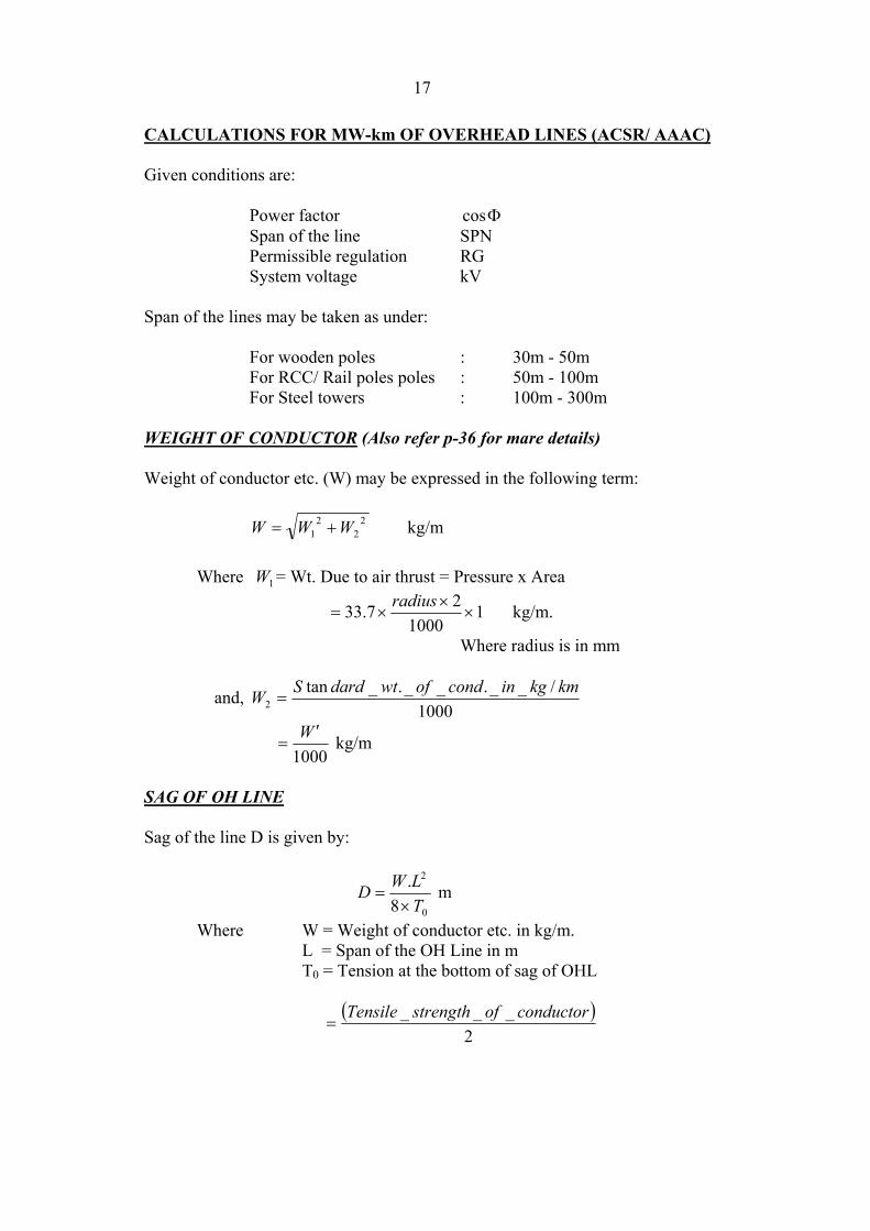
CALCULATIONS FOR MW-km OF OVERHEAD LINES (ACSR/ AAAC) Given conditions are: Power factor Φcos Span of the line SPN Permissible regulation RG System voltage kV Span of the lines may be taken as under: For wooden poles : 30m - 50m For RCC/ Rail poles poles : 50m - 100m For Steel towers : 100m - 300m WEIGHT OF CONDUCTOR (Also refer p-36 for mare details) Weight of conductor etc. (W) may be expressed in the following term:

22

21 WW +=W kg/m

Where W = Wt. Due to air thrust = Pressure x Area 1

11000

27.33 ××

×=radius kg/m.

Where radius is in mm

and, 1000

/__.__._tan2

kmkgincondofwtdardSW =

1000W ′

= kg/m

SAG OF OH LINE Sag of the line D is given by:

0

2

8.TLWD

×= m

Where W = Weight of conductor etc. in kg/m. L = Span of the OH Line in m T0 = Tension at the bottom of sag of OHL

( )2

___ conductorofstrengthTensile=

18

SPACING BETWEEN CONDUCTORS Spacing between conductors SP is given by the following empirical formula:

+=

150VDSP m (For Aluminium)

Where D = Sag of OHL in m, V is voltage in kV. Equivalent spacing is given by d = 1.26 × SP (For Horiz. conductors) RESISTANCE OF CONDUCTOR Resistance of the conductor is given by:

a

lalr ×

=×=86.17

ρ in ohms [ for copper kmmm /.86.17 2Ω=ρ

kma

/86.Ω

17=

Resistance at a temperature t0 C is given by:

++

=205.241

5.241. trrt Where r is resistance at 200C

Now, MW-km is given by:

MW-km = [ ]( )Φ+Φ

Φsin.cos..100(%)Re.2

lxrgV cos per phase

Where V is phase voltage in kV.

MAXIMUM ACTIVE AND REACTIVE POWER THROUGH AN OVERHEAD LINE

r x

Loa

d

Neutral

sE r

I

E

19

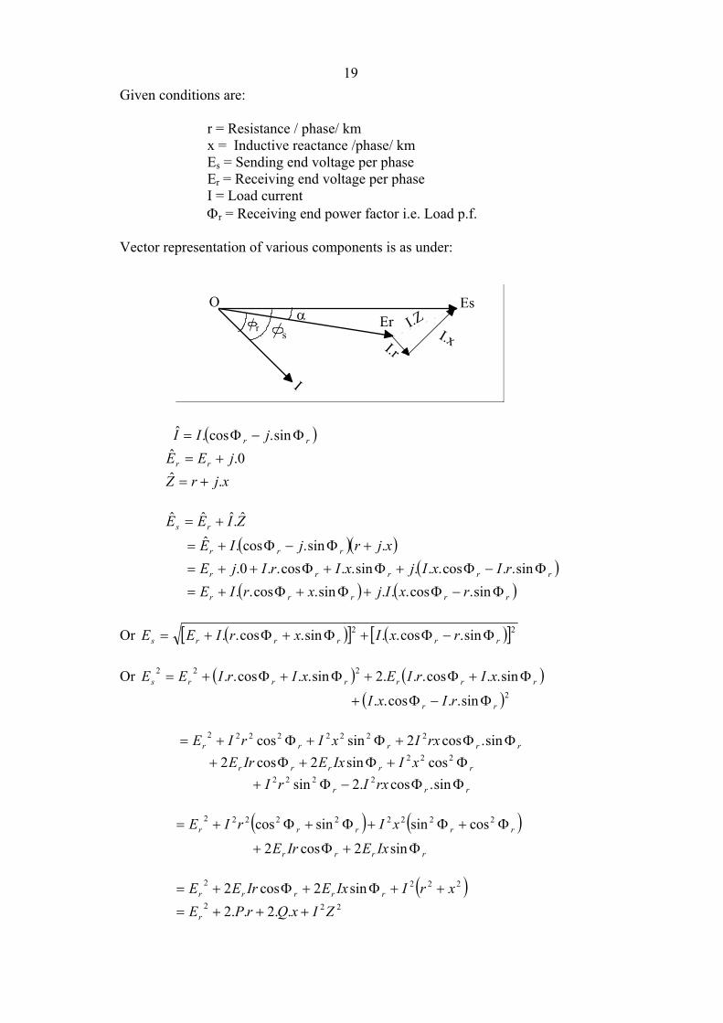
Given conditions are: r = Resistance / phase/ km x = Inductive reactance /phase/ km Es = Sending end voltage per phase Er = Receiving end voltage per phase I = Load current Φr = Receiving end power factor i.e. Load p.f. Vector representation of various components is as under:

EsErI.r

I.x

I

O

s

α I.Zr

II = ( )rr j Φ−Φ sin.cos.ˆ

0

( )

)

.ˆ jEE rr +=

xjrZ .ˆ += ZIEE rs

ˆ.ˆˆ +=

( ) xjrjIE rrr .sin.cos.ˆ +Φ−Φ+=

( )rrrrr rIxIjxIrIjE Φ−Φ+Φ+Φ++= sin..cos...sin..cos..0. ( ) ( rrrrr rxIjxrIE Φ−Φ+Φ+Φ+= sin.cos...sin.cos..

Or ( )[ ] ( )[ ]22 sin.cos..sin.cos.. rrrrrs rxIxrIE Φ−Φ+Φ+Φ+E = Or EE =2 ( ) ( )rrrrrrs xIrIExIrI Φ+Φ+Φ+Φ+ sin..cos...2sin..cos.. 22

( )2sin..cos.. rr rIxI Φ−Φ+ rrrrr rxIxIrIE ΦΦ+Φ+Φ+= sin.cos2sincos 22222222

rrrrr xIIxEIrE Φ+Φ+Φ+ 222 cossin2cos2 rrr rxIrI ΦΦ−Φ+ sin.cos.2sin 2222

E += 2 ( ) ( )rrrrr xIrI Φ+Φ+Φ+Φ 22222222 cossinsincos

rrrr IxEIrE Φ+Φ+ sin2cos2 2E += ( )222sin2cos2 xrIIxEIrE rrrrr ++Φ+Φ

2E += 22..2..2 ZIxQrPr ++

20

Where EP = -> Active power rr I Φcos Q -> Reactive power rr IE Φ= sin..

Z = 22 xr + -> Impedance

Therefore, ( 222

222 ..2..2 xr

EQPxQrPE

rrs +

++++= )2E (i)

Considering P and Q as variables. Maximum value of P can be found by

differentiating the above equation with respect to Q and equating dQdP to zero.

Differentiating w.r.t. Q:

+

++++= Q

dQdPP

Exrx

dQdPr

r

222200 2

22

When 0dQ

=dP then,

( )QE

xrxr

202000 2

22

++

+++=

Or 02 2

22

=+

+rE

xrQx2

Or 22

2.xr

Ex r

+−

Q =

Or 2

2 .Z

xErQ =

Putting this value of Q in equation (i) above, the maximum active power Pmax

can be found as under:

0..

.2..2 2

22

4

242

2

222 =

+

+−

−−−−

r

rrrs E

xrZ

xEP

ZxE

xrPEE

Or 0....2..2 2

2

4

24

2

22

2

222 =−−+−−

r

r

r

rrs E

ZZ

xEE

ZPZ

xErPE2E

Or 0....2 2

22

2

222 =+−−−

ZxE

EZPrPE r

rrs

2E

Or 01Pr2 2

222

2

22

=

−+−+

ZxEE

EZ

rsr

P

Or 0.Pr2 2

222

2

22

=+−+Z

rEEE

Z rs

r

P

21

This is a quadratic equation in P. Solving this, we get:

2

2

2

222

2

22

.2

.442

r

rs

r

EZ

ZrEE

EZrr

P

+−−±−

=

Neglecting the negative value of P, we get Pmax = P as under:

−= r

EE

ZZEP

r

sr .2

2

max Watts/ phase

Assuming r = Z in the above equation, maximum power Pmax can be

expressed as under:

−=

r

rsr

EEE

ZZEP .2

2

max Watts/ phase

gulationZE

P r Re2

2

max ×= Watts/ phase

And,

2

2

max.

ZxEr−=Q VAr/ phase

Power factor angle is also given by:

Φ Active Power P

ReactivePower

QApparent Power

r

22_

_cosQP

PPowerApparent

PowerActiver

+==Φ

IV

IV

r

rr

.cos.. Φ

= Where Vr = Receiving voltage

Therefore,

22

cosQP

Pr

+=Φ

22

CABLE SELECTION Cable selection can be done on the following grounds: 1. Considering the rms load current through the cable. 2. Considering the voltage regulation 3. Considering the fault current i.e. the symmetrical breaking

capacity. 1. SELECTION BASED ON RMS CURRENT The effective current for calculating the cable size is taken as under: Maximum load current through the cable is Where P = load in kW V = L-L voltage in kV Φ = Load power factor Average current Iav is given by:

..FL

II m

av = Where L.F. = Load Factor (Daily/ Monthly/ Annual)

Form factor (FF) is calculated from the given load factor with the help

of following Table:

LF 0.1 0.15 0.2 0.3 0.4 0.5 0.6 0.7 0.8 0.9 1 FF 2.3 1.93 1.77 1.52 1.37 1.25 1.17 1.1 1.06 1.03 1

RMS current is then calculated as under: FFLFII mrms ..= 2. SELECTION BASED ON VOLTAGE REGULATION The voltage regulation limits, as per the Indian Electricity Rules 1956,

are as under: For low voltages upto 250V + 6% For medium voltages upto 650V + 6% For high voltages upto 33kV between - 6% & + 9% For extra high voltages >33kV between - 10% & +12.5% Frequency variation limits for the supply system is + 3%.

23

EFFECT OF TEMPERATURE RESISTANCE The dc resistance of a conductor varies with temperature. The following

empirical formulae give the resistance at any other temperature. It may be noted that normally resistances are given in tables at 200 C.

(a)

++205.241

5.24120

tt = rr Where t is temp. in 0C

is resistance at 2020r 0C is temp. at ttr

0C (b) ( )[ ]201 2020 −+= trrt α Where α20 = 0.004 per 0C = temperature coefficient INDUCTANCE Effect of temperature on the inductive reactance is negligible and can

be ignored for all practical purposes. CAPACITANCE In view of the short length of cables, normally under use, the

capacitance has not been considered in its equivalent network. VOLTAGE REGULATION: Voltage drop is given by Drop = current ZIimpedance ˆ.=×

Where I and are vectors. ˆ Z If =V Sending end voltage then, s

V ZIVsrˆ.ˆˆ −=

And,

Percentage regulation = 100ˆ

ˆˆ×

−

s

rs

V

VV

3. SELECTION BASED ON FAULT CURRENT Minimum cross sectional area of the cable is given by:

K

tIKcsa sct ××

=min sq.mm.

24

Where Isc is 3 phase short circuit current in kA, t is total break time of C.B. (Opening time + Arcing time) in second, Kt is coefficient corresponding to break time t and K is thermal admissible strength of conductor material (K=116.80 for Cu and K=77.80 for Al).

Break time varies between 0.2 sec and 1.2 sec, Kt is normally taken

between 1 and 1.1 for circuit breakers. Symmetrical short circuit current is calculated by reducing the given

network to an equivalent impedance for the worst condition i.e. a 3 phase short circuit.

Fault level at a point in the network is given by: Fault Level = scl IV. .3 MVA When Vl is in kV & Isc is in kA

LOSSES IN CABLES (i) Conductor I2.r loss or Copper loss (ii) Dielectric loss (iii) Seath loss CONDUCTOR I 2.r LOSS (COPPER LOSS) As already discussed the resistance of cable conductor at the working

temperature is calculated. Let the calculted resistance be rt. To allow for stranding of conductors 2% is added to rtc. To further allow the multicore structure of cable 2% is further added in the resistance. Finally, the resistance at a temperature t is given by:

tct rr ××= 02.102.1 Losses are calculated with rms current and not with maximum current

or average current. RMS current is given by: lfrms KKII ..max= Where Kf and Kl are form factor and load factor respectively. And maximum load current Imax is given by:

Φ

=cos..3max V

PI

25

DIELECTRIC LOSS The charging current of the cable has two components as shown below:

Given conditions:

δ

φd

Id

Ic

I0

V

I0= Charging current Ic= Capacitive current Id= Dielectric loss component of charging current V = Voltage (L-N) δ = Dielectric loss angle φd = Dielectric p.f. angle To find: Dielectric loss

From the above vector diagram:

ω

ω

VC

C

VXVI

c

===

.10

dd II Φ= cos.0

Dielectric loss = V.Id = V.I0.cosφd Dielectric loss V= 2 dC Φcos.ω

When δ is small δω sin.2CV= δδ ≈sin Therefore, Dielectric Loss 2V= Watts/ phase δω.C And, Total dielectric loss Watts δω..3 2CV=

The value of δ or the dielectric power factor angle or cable power factor varies with temperature. Typical values may be considered for δ at a suitable temperature.

dΦcos

Power factors of cables at 450 C are as under:

Sl.no. VOLTAGE Power factor of the cable

1 0.415 kV 0 2 0.55 kV 0 3 3.3 kV 0.007 4 6.6 kV 0.01 5 11 kV 0.012 6 33 kV 0.024

26

SEATH LOSSES IN CABLES Sheath loss is given by the following empirical formula by Arnold:

Sheath loss =

×

−9

222 1078

dr

RI m

s

ω Watts per phase

Where I = Current through the conductor, rm = Mean sheath radius, Rs = Sheath resistance in , Ω d = Distance between conductors, Note: rm and d should be in the same units. However, for all practical purposes, sheath losses are taken equal to 2% of the

total losses in the cable.

RESISTANCE, INDUCTANCE, CAPACITANCE, SAG AND CONDUCTOR SPACING CALCULATIONS OF

OVERHEAD LINES WITH ACSR CONDUCTORS

1. SAG OF OVERHEAD LINES: While calculating sag of an overhead line, it is assumed that during severe

conditions the wind velocity may go upto 40-45 km/hour thereby developing a pressure of about 33.7 kg/m2.

Effective weight/ tension is due to: (a) Dead weight of the conductor, w1 (b) Due to the tension developed during windy days, w2

l

2rConductor

Dead weight w1 can be obtained from tables. Thrust due to blowing wind can be found as under: Let r = Radius of the conductor, l = Length of the conductor,

Thrust = Pressure x Area of exposure per running m

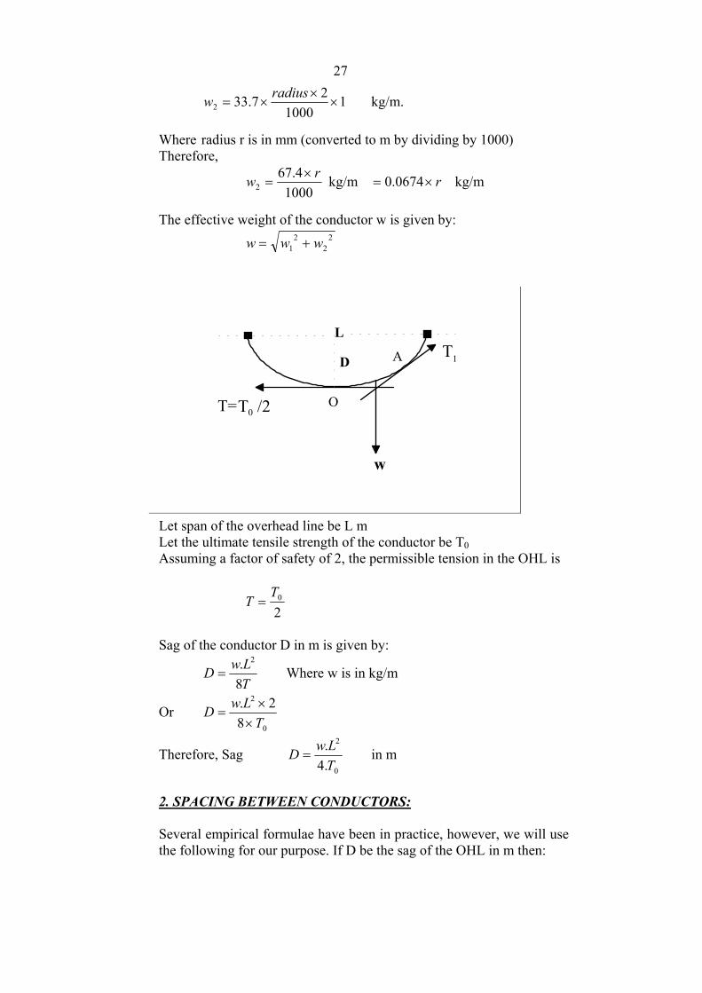
27

11000

27.332 ××

×=radiusw kg/m.

Where radius r is in mm (converted to m by dividing by 1000) Therefore,

1000

4.672

rw ×= kg/m kg/m r×= 0674.0

The effective weight of the conductor w is given by:

22

21 www +=

L

T=T0 /2

T1

w

A

O

D

Let span of the overhead line be L m Let the ultimate tensile strength of the conductor be T0 Assuming a factor of safety of 2, the permissible tension in the OHL is

20T

=T

Sag of the conductor D in m is given by:

TLwD

8. 2

= Where w is in kg/m

Or 0

2

82.

TLw×

×D =

Therefore, Sag 0

2

.4

.TLwD = in m

2. SPACING BETWEEN CONDUCTORS: Several empirical formulae have been in practice, however, we will use

the following for our purpose. If D be the sag of the OHL in m then:

28

d

d3

2

d1

Spacing = 150

75. kVVD +0 in m for copper

Spacing = 150

kVVD + in m for aluminium

EQUIVALENT SPACING If the conductors are placed equilaterally/ laterally (Horizontal or

Vertical) or in any other shape, the equivalent spacing d is given by:

( )31

321 .. dddd = = d ( For equilaterally placed conductors) = 1.26 d (For vertical or horizontally placed conductors) We will now, find the inductance and capacitance by using the above

value of equivalent spacing. 3. INDUCTANCE OF 3 phase OHL Inductance L per phase is given by:

710ln.25.0 −×

+=

rdL Henry/ m

Where d = Equivalent spacing in mm r = Radius of cond. in mm. Also, Inductive reactance per phase is given by: Xl = 2.π.f.L

710ln.25.050 −×

+×

rd

π2 ×= m/Ω

Or

+×= −

rdln.25.010 2πX l km/Ω

4. CAPACITANCE OF 3 phase OHL

Capacitance of the OHL between one phase and neutral is given by:

rdln

2πε=C Where 910

361 −×π

=ε

29

rd

rd ln1018

1

ln

36102

9

9

××=

×=

−

ππ

Farad per m

rdln1018

13 ××

= mF /µ

rd

Cln18

1

×= kmF /µ

5. RESISTANCE OF OHL Resistance per phase of a conductor is given by:

al

=ρ Where = Sp. resistance of cond. material ρ

a = Cross sectional area of conductor l = Length of OHL r = Resistance in Ω For copper at 20°C kmmm /.86.17 2Ω=ρ For Aluminium =ρ at 20°C kmmm /.70.28 2Ω For Steel at 20°C kmmm /.0.178 2Ω=ρ For our purpose, in ACSR, we will take resistivity of aluminium as 28.7

and 17.86 for its copper equivalent. Moreover, the variation of resistance with temperature is governed by:

++

=205.241

4.24120

trrt Where r20 is resistance at 20°C

And also by: Where resistance temp. coefficient ([ 201 2020 −+= trrt α )] α for copper 0038.020 = = 0.0040 for aluminium MOST ECONOMICAL POWER FACTOR OF A SYSTEM Given conditions may be like this: Active power in kW PA Power factor angle of load φ1 Power factor angle after improvement φ21 Maximum demand rate/kVA MDR Cost of pf improvement plant /kVAr CC Rate of interest & depreciation id Rate of incentive for high pf /month HPF Limit above which pf incentive is allowed HPFL kW rating of the highest single motor/ load MkW

30

It is to explore a condition for most economical pf of the system

without loosing the stability of the system. For this we will define two terms viz.: (1) Desirable power factor and (2) Most suitable power factor DESIRABLE POWER FACTOR Desirable power factor is that most economical power factor which

does not allow the system to cross the plus unity point, avoiding leading power factor, on switching off the highest motor or electrical load running within the system.

MOST ECONOMICAL POWER FACTOR Most economical power factor is that power factor which is calculated

with due consideration of cost of reactive kVAr versus incentive given on high power factor. This ignores the system stability and other demerits of leading power factor.

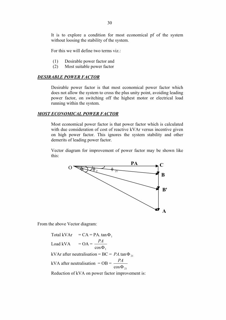
Vector diagram for improvement of power factor may be shown like

this:

φ1 φ 2 φ 21Ο C

B

B'

A

PA

From the above Vector diagram: Total kVAr = CA = PA. tan 1Φ

Load kVA = OA = 1cosΦ

PA

kVAr after neutralisation = BC = 21tan. ΦPA

kVA after neutralisation = OB = 21cosΦ

PA

Reduction of kVA on power factor improvement is:

31

OA-OB 211 coscos Φ

−Φ

PA=

PA

Annual saving due to kVA reduction will be equal to (kVA reduced) x (M.D. rate/kVA/month) x 12

12coscos 211

××

Φ

−Φ

= MDRPAPA (i)

kVAr neutralised = PA 211 tan.tan. Φ−Φ PA Cost of neutralised kVAr/ annum is given by:

( )100

_ idCCdneutralizekVAr ××=

( 211 tan.tan.100

.Φ−Φ×= PAPAidCC )

)

(ii)

Incentive for high power factor is HPF% /month means that HPF rupees

per month is given as incentive for 1% increase in power factor. Since the limit beyond which incentive is given is HPFL, the annual

incentive will be: Annual incentive = ( )×MD ( 12/_ ××− monthrateIncentiveHPFLpf

( ) 12coscos 21

21

××−Φ×Φ

HPFHPFL=PA

12cos

.

21

××

Φ

HPFLHPFLPA −= PA

12cos

121

×××

Φ

− HPFLPAHPFL= (iii)

Equating the cost involved and saving we get saving S as under:

( ) ( )211 tantan100

..Φ−Φ×=

PAidCCS

12cos

1cos

1

211

×××

Φ

−Φ

− MDRPA

12cos

121

×××

Φ

−− HPFPAHPFL (iv)

Now, saving will be maximum when 01

=ΦddS . Equating the above

equation no. (iv) w.r.t. Φ we get: 21

32

( )212

2

sec0100

..Φ−=

ΦPAidCC

ddS

( )2121 tan.sec012 ΦΦ−×××− MDRPA ( ) 12tan.sec.0 2121 ×××ΦΦ−− MDRPAHPFL

Or 212121

2

2

tan.sec..12100

sec...ΦΦ×+

Φ=

ΦMDRPAPAidCC

ddS

0tan.sec12 2121 =ΦΦ××××+ HPFLHPFPA

Or 2121 tan12

100sec..

Φ××+Φ MDRid

−CC

0tan12 21 =Φ×××+ HPFLHPF

Or 0cos

sin...12cos

sin12100

.

21

21

21

21 =Φ

Φ−

ΦΦ××

−HPFLHPFMDRidCC

Or 0sin12sin12100

.2121 =Φ×××−Φ××− HPFLHPFMDRidCC

Or ( )100

.sin 21idCCHPFLHPFMDR =++Φ×12

Or ( )HPFLHPFMDRidCC

++=Φ

1200.

21sin

From here, we can find the MOST ECONOMICAL POWER FACTOR

as under: 21cosΦ

212

21 sin1cos Φ−=Φ NOTE: It may be noted that supply companies normally allow power factor

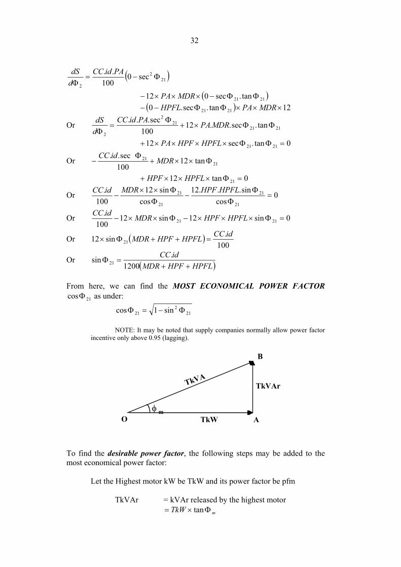
incentive only above 0.95 (lagging).

φ mTkW

TkVArTkVA

O A

B

To find the desirable power factor, the following steps may be added to the

most economical power factor: Let the Highest motor kW be TkW and its power factor be pfm TkVAr = kVAr released by the highest motor mTkW Φ×= tan

33

m

mTkWΦΦ

×=cossin

ΦΦ−

×=m

mTkWcos

cos1 2

Or

−×=

pfmpfm

TkW21

TkVAr

Total kVAr = kVAr at most economical power factor + kVAr released by highest motor. Or B (Refer drawing at p-30) BBBCC ′+=′

−+Φ=

pfmpfm

TkWPA2

211

tan.

Or OC

CB′=Φ 2tan

PA

pfmpfm

TkWPA

−+Φ

=

2

211

tan.

Hence, the most suitable or the DESIRABLE POWER FACTOR of the system is given by: 2cosΦ

2

22tan11cos

Φ−=Φ

CORONA LOSS

Corona is a phenomenon which occurs at high voltages in overhead lines when the potential gradient reaches a critical value of about 30 kV/cm(Peak) equivalent to 21.1 kV(rms). At this voltage the air in between ionises. Corona is associated with a power loss. The voltage at which this phenomenon starts with a hissing sound is known as Disruptive Critical Voltage while the voltage at which this becomes just visible is known as Visual Critical Voltage. The corona is also affected by the smoothness of the conductor, atmospheric pressure, frequency, radius of conductor, spacing between conductors and temperature. The following empirical formulae have been used for estimating various voltages and loss.

34

Disruptive Critical Voltage

××=

rdrVd ln1.21

Where r and d are in cm. and Vd in kV

For a three phase system,

×××=

rdrVd ln1.213

Considering the effects of conductor smoothness, atmospheric pressure and temperature the equation finally comes as:

××××=

rdmrVd ln1.21 0 δ kV(rms)/phase

Where air density factor t

B+

=273

93.3δ

B = Atmospheric pr. in cm of Hg. t = Temperature in °C m0 = Irregularity factor = > 0.80 to 0.87 for ACSR conductors Assuming m0=0.84 and δ i.e. m we get, 9762.0= 82.0.0 =δ

×××=

rdrVd ln82.01.21 kV(rms)/phase

××=

rdr ln302.17 kV(rms)/phase

Power loss due to CORONA is given by the following empirical formula:

( )( ) 52 10254.242 −×

×−+=drVEfP dphδ

kW/km of conductor

If ln be the length of OHL in km, frequency f=50Hz and air density coefficient δ be taken as unity then for a three phase line the losses may be taken as:

( ) 52 10754.2423 −×××=×××= ndph ldrVEP kW

VOLTAGE REGULATION AND DROP IN CABLES

Sendingend

ReceivingendResistance= r, Reactance= x

Length= l kmVoltage= Vs Load= P in kW

I

Voltage = Vr

Cable

35

Given conditions are: Receiving end voltage Vr in kV 3 phase load in kW P Load power factor cosφ Resistance & Reactance r, x Length of cable in km l Capacitance of the cable Neglected. To find the following: Sending end voltage Vs Voltage drop in the cable I.Z Voltage regulation Reg Sending end power factor cosφs The vector diagram of the system is as shown hereunder: Vs

Vr

I.r I.x

I

O

s

= I cos φ - j I sin φ I= Iφcos3 rV

P

r' = Resistance/ phase/ km x'= Reactance/ phase/ km r1 = Resistance/ phase = r' .l x = Reactance/ phase = x'.l Impedance per phase= = rZ 1+j.x Voltage drop = I ))(sincos(ˆ

1 jxrjIIZ +−= φφ

Resistance at t0 C is given by: r = r1

++205.241

5.241 t

Replacing r1 by r, the voltage drop is: Volts I )sincos()sincos(ˆ φφφφ rxjIxrIZ −++= Sending end voltage is given by:

1000

)sin.cos.(..1000

)sin.cos.(ˆ.ˆˆ Φ−Φ+

Φ+Φ

+=+=rxIjxrIVZIV rrsV

Sending end power factor s

rs V

IrV )1000/(coscos +Φ=Φ

Regulation = 100×−

s

rs

VVV

36

SAG AND TENSION IN OVERHEAD TRANSMISSION LINES The tension equation of an overhead line is given by:

( )2424

(2

22

02

1221

21

20

2

122

2λ

λαλ qWl

ttTqWl

TT =

−−

−−T (i)

Where T = Tension at temperature t1 1 °C = Tension at temperature t2T 2 °C = Span of OHL in m l = Weight of bare conductor in kg/m 0W = Loading factor at temperature t1q 1 °C = Loading factor at temperature t2q 2 °C = Coefficient of linear expansion /°C α = Initial and final temperatures in °C 21, tt

Let A

W0=δ Where A = Conductor CS Area in sq. m.

AfT .11 = Where f1= Stress at t1 °C temperature AfT .12 = Where f2= Stress at t2 °C temperature

Substituting these values in equation (i):

( )24

....24

.....(.2

2222

12221

21

222

1222

2AEqAlAEtt

AfAEqAlAfAfAf δ

αδ

=

−−

−−

or, ( )2424

..(2

222

1221

21

22

122

2EqlEtt

fEqlfff δ

αδ

=

−−

−−

or, (ii) [ ]( ZEtKff =−− ..22

2 α )

Where

−= 21

21

22

1 24...

fEqlf δK

24

22

22 Eql δ=Z

Finally, the tension equation (i) reduces to (ii). This equation takes into account the effect of temperature, conductor load and wind pressure. EFFECTIVE WEIGHT OF CONDUCTOR: Weight of conductor etc. (W) may be expressed in the following term:

37

21

20 WW +=W kg/m

Where W = Dead weight of conductor, 0

W = Weight due to wind. 1

The dead weight of conductor can be found from tables. IS-398 may be referred if necessary. The effective wind pressure, if not given, can be obtained from the procedure led down in IS-802(Part-1/Sec-1):1995. The procedure is summarised below:

(a) Select reliability level- For normal towers upto 400kV it is 1. (b) Select the basic wind velocity Vb as per clause 8.1 & referred map. (c) Calculate meteorological reference wind speed VR

375.10

bbR

VKV

==V

(d) Find design wind speed as per clause 8.3, given by: 21 KKVV Rd ××= Where K1 = Risk coefficient (Value as given in Table-2of IS:802[P1/S1]) K2 = Terrain roughness coefficient (Value as given in Table-3of IS:802[P1/S1])

(e) Design wind pressure as per clause 8.4, given by: 26.0 dd VP ×= Where Pd = Design wind pressure in N/m2 Vd = Design wind speed in m/sec Design wind pressure can be calculated or else can be directly taken from Table-4 of the referred IS:802(P1/S1) for given Reliability level and Terrain category. Now, wind load in kg/m can be calculated from the formula given for this purpose in clause 9.2 of the referred IS:802(P1/S1), given by:

81.9

cdcdwe

GdCPF

×××= kg/m

Where Pd = Design wind pressure in N/m2 Cdc = Drag coefficient (1 for conductor and 1.2 for ground-wire) d = Diameter of conductor in m Gc = Gust response factor, given in Table 7 of the referred IS:802. Gust response factor takes into account the turbulence of the wind and the dynamic response of the conductor. The value of Gust factor corresponds to:

(a) Specific Terrain category, (b) Height above ground and (c) Ruling span

38

The average height of conductor/ ground-wire above ground is taken as height of the upper-most conductor upto clamped point, below insulator, less two-third of the sag at minimum temperature and no wind. Ruling span L of a section having spans of L1, L2, L3, … is given by:

..

..

321

33

32

31

++++++

=LLLLLLL

Sag S may now be calculated from the formula:

spanRulingatSagspanRulingspanActual ___

__

2

×

=S

FACTOR OF SAFETY FOR CONDUCTORS:

1. As per Indian Electricity Rules 1956, the minimum factor of safety for conductors shall be taken as 2 based on their ultimate tensile strength.

2. As per IS:802(P1/S1) the tension limits for Conductors/ ground-wires at everyday

temperature and without external load, should not exceed the following limits:

i. Initial unloaded tension35% of UTS ii. Final unloaded tension25% of UTS

Provided that the Ultimate Tension under everyday temperature and 100% design wind pressure, or minimum temperature and 36% design wind pressure does not exceed 70% of the UTS of the conductor/ ground-wire.

3. The IS:802(P1/S1):1995 in its ‘Foreword’ says like this: Some of the major modifications made in this section are as under:

a) Concept of maximum working load multiplied by the factors of safety as per IE Rules has been replaced by the ultimate load concept.

4. The 3rd of the above three guidelines suggests that there is no need of taking any

factor of safety as per IE Rules because it is being taken up in re-assessing the value of conductor load (dead load of conductor and wind load) as calculated on the guidelines given in IS:802(P1/S1):1995. The suggested method of finding re-assessed load in the IS has no-where defined the ‘Ultimate Load’.

However, if at all, it is taken into consideration, then not only the limit of factor of safety 2 (50% of UTS) changes but also the other limit 35% at 36% wind load should change accordingly.

39

VOLTAGE DROP & REGULATION IN OVERHEAD LINES (WHEN SENDING END VOLTAGE IS KNOWN) GIVEN: A load of 5000 kW of power factor 0.86 (lagging) is connected at the receiving end of a 6 km long, 3 phase, 11 kV overhead line with ACSR LYNX conductor. The sending end voltage is 11 kV, conductor temperature is 40°C, spacing between horizontally led conductors is 700mm. Annual load factor is 60%. TO FIND: Receiving end voltage, sending end of, regulation, voltage drop, maximum losses, rms losses, line efficiency, resistance, reactance, capacitance, surge impedance, load current, disruptive critical voltage, corona loss and annual energy losses. CALCULATIONS: From tables, we find:

radius of cond. rd=9.77mm, resistance/ km = 0.1554, reactance/ km= 0.261 cs area of ACSR LYNX = 183 mm2 (Aluminium) , 110 mm2 (Copper equiv.) Current carrying capacity of conductor =360 A

Capacitance of the line is:

phaseF

rd

lC

d

/078.0

77.9700ln18

6

ln18µ=

×

=

×

=

Reactance of the line: x = 0.261 × 6 = 1.566 Ω/phase Resistance of the line at the given temperature:

0037.161673.065.261405.2411554.0 =×=×

+×=r Ω/phase

Given sending end voltage 63513

11000==sV V

Active power 67.16663

5000==P kW

Reactive Power kVAr 9895934.067.1666tan. =×=Φ= PQ 86.0cos[ =ΦQ

Receiving end voltage is given by:

2

42 BAAAAVr−±

=

Where 2VAA −= )..(2000 xQrPs +

Φ×

2

622

cos10.Z

=PB

40

Now, )..(20002 xQrPVAA +×−= = )6261.098961673.067.1666(200063512 ××+×××− = 33.89 × 106

( ) ( )[ ] 62

2226

2

22

1086.0

6261.061673.067.1666410cos

.44 ××+×××

=×Φ

=ZPB

= 121098.51 × Therefore,

2

1098.511089.331089.33 121226 ×−×±×=Vr

3102

12.3389.33×

±=

= 5788.13 V )(5788 Say→=

L-L Voltage in kV is: 025.101000

35788=

× kV

Load Current is given by:

82.33486.057881067.1666

cos.

3

=××

=Φ

=rV

PI Amps.

Sending end power factor is:

s

rs V

lrIV ..cos.cos +Φ=Φ [Refer vector diagram of the text part

837.06351

61673.082.33486.05788=

××+×=

Voltage Regulation is given by:

%86.81006351

57886351100Re =×−

=×−

=s

rs

VVV

g

Voltage drop per phase is given by: ( ) ( )22 sin.sin.cos.cos.. Φ−Φ+Φ−Φ= rssrss VVVVZI

( ) ( )8.622

51.05788547.0635186.05788837.06351 22

=

×−×+×−×=

L-L Voltage drop is thus: 69.107838.622 =×= Also, it can be arrived at by:

Voltage drop per phase is: I.Z = 334.82 × (0.1673 × 6 + j 0.261 × 6) = 622.4 V

41

L-L Voltage drop 107834.622 =×= V Line losses in terms of kW is given by: ( )2__ FFLFLossesMaximumLossesRMS ××=

( ) 2//3_ FFLFphaseOutputphaseInputLossesRMS ×−×= ( )

) =

( ) ( )( ) (

35.166)17.16.0(56.337

1017.16.082.33486.05788837.063513

cos.cos.3

2

32

2

=××=

×××××−××

×××Φ−Φ×=−

FFLFIVV rss

Annual Energy Loss is given by: sAnnualHourLossesRMSLosses ×= _ =166.35 × 365 × 24 kWh =1457247 kWh Overhead line efficiency is given by:

%68.93100837.0635186.05788100

__

=×××

=×=InputLine

OutputLinelineη

Surge impedance of the line:

fCx

fCfL

CLSI

πππ

222

===

Ω=××××× 75.252

078.0502106261.0 6

π=

Disruptive Critical Voltage is given by:

××××=

rddrdmVd ln1.21 0 δ

×××

77.9700ln977.082.01.= 21 [Since 82.00 =×δm

= 72.2 kV VOLTAGE DROP & REGULATION IN OVERHEAD LINES (WHEN RECEIVING END VOLTAGE IS KNOWN) GIVEN: A load of 5000 kW of power factor 0.86 (lagging) is connected at the receiving end of a 6 km long, 3 phase, 11 kV overhead line with ACSR LYNX conductor. The receiving end voltage is 11 kV, conductor temperature is 40°C, spacing between horizontally led conductors is 700mm. Annual load factor is 60%.

42

TO FIND: Sending end voltage, sending end current, sending end pf, regulation, voltage drop, line efficiency, rms losses, maximum losses, receiving end load current, resistance, reactance, capacitance, Dr. Steinmetz capacitance currents, disruptive critical voltage, corona loss and annual energy losses CALCULATIONS: From tables, we find:

radius of cond. rd=9.77mm, resistance/ km = 0.1554, reactance/ km= 0.261 cs area of ACSR LYNX = 183 mm2 (Aluminium) , 110 mm2 (Copper equiv.) Current carrying capacity of conductor =360 A

Capacitance of the line per km is:

phaseF

rd

lC

d

/078.0

77.9700ln18

6

ln18µ=

×

=

×

=

Reactance of the line: x = 0.261 × 6 = 1.566 Ω/phase Resistance of the line at the given temperature:

0037.161673.065.261405.2411554.0 =×=×

+×=r Ω/phase

Given receiving end voltage 63513

11000==Vp V

Referring to the text diagram:

Reactance Ω=××

×== 244754

078.01001066

6

6

πϖCCt =1ϖ

x

Reactance Ω=××

×== 61188

078.02100103

23

321 6

πϖCCm =ϖ

x

Current 15.30586.0113

5000cos..3

ˆ =××

=ΦV

kW=I

Or, 015.305ˆ jI += Voltage Vr = ( ) ( 51.086.06351sincosˆ jjVr +×=Φ+Φ ) = 5461.9+j3239

43

Capacitor-1 current is given by:

0223.00132.0244754

32399.5461ˆˆ

1 jjjxV

jIt

rc +−=

+==

= 0.0259 A (Abs.) Line Current-1 is given by: 0223.0137.3050223.00132.015.305ˆˆˆ

11 jjIII cs +=+−=+= Voltage drop in receiving half line is:

( )

+×+=

220223.0137.305ˆ.ˆ

1xjrjZI s

= ( )(

)(76.28394.238119.153

783.0501856.00223.0137.305

Absolutej

jj

→=+

++= )

Mid point voltage is given by: halfreceivingindropVV rm ___ˆˆ += = 5461.9 + j3239 + 153.119 + j238.94 = 5614.85 + j3479.7 Capacitor-2 current is given by:

)(108.00918.005687.061188

7.347985.5614ˆˆ

2 AbsolutejjjxV

jIm

mc →=+−=

+==

Line Current-2 is given by: 212

ˆˆˆcss III +=

= 305.137 + j0.0223 + j0.0918 - 0.05687 = 305.08 + j0.1141 = 305.08 (Absolute) Voltage drop in sending half line is:

( )

+×+=

22114.008.305ˆ.ˆ

2xjrjZI s

( )(

)

94.2380192.153783.0501856.0114.008.305

jjj

+=++=

= 283.74 (Absolute) Sending end voltage is given by: linetheindropVV ms ___ˆˆ += = 5614.85 + j3479.7 + 153 + j238.94 = 5767.87 + j3718.68 = 6862.7 (Absolute) (Phase voltage) = 11.887 kV (Line to line voltage)

44

Capacitor-3 current is given by:

244754

68.371887.5767ˆˆ

3jj

xV

jIt

sc

+==

Or, )(02804.002357.00151935.0ˆ3 AbsolutejI c →=+−=

Sending end current is given by: 01519.00236.0114.008.305ˆˆˆ

32 −++=+= jIII css

= 305.068 + j0.1376 = 305.07 (Absolute) Vector Angle between Vθ s components is given by:

radiansin

VofcomponentHorizontVofcomponentVertical

s

s

_572657.087.576768.3718tan

______

tan

1

1

→=

=

=

−

−

Angle between Is and I is given by:

000451.0068.305

1376.0tan 1 =

= −α

Therefore, sending end power factor angle is: 5722056.0000451.0572657.0 =−=Φ s

Or, 8407.0cos =Φ s

Percentage voltage regulation is given by:

%46.71006863

63516863100ˆ

ˆˆRe =×

−=×

−=

s

rs

V

VVg

Line losses in kW is given by: Line losses = Line Input – Line Output

( )3= ( )

3.28086.015.30563518407.007.3057.6862

cos..cos..3

=××−×××

Φ−Φ×= IVIV rsss

Line losses (rms) in kW is given by: ( )2__ FFLFLossesMaximumLossesRMS ××=

( )23.280_ FFLFLossesRMS ××=2

( )kW→=××=

14.13817.16.03.280

Annual Energy Losses is given by: sAnnualHourLossesRMSLosses ×= _ =138.14092 × 365 × 24 kWh =1210114 kWh

45

Overhead line efficiency is given by:

%69.941008407.007.305686386.015.3056351100

__

=×××××

=×=InputLine

OutputLinelineη

Surge impedance of the line:

fCx

fCfL

CLSI

πππ

222

===

Ω=××××× 75.252

078.0502106261.0 6

π=

Disruptive Critical Voltage is given by:

××××=

rddrdmVd ln1.21 0 δ

×××

77.9700ln977.082.01.= 21 [Since 82.00 =×δm

= 72.2 kV Voltage drop/ phase is given by:

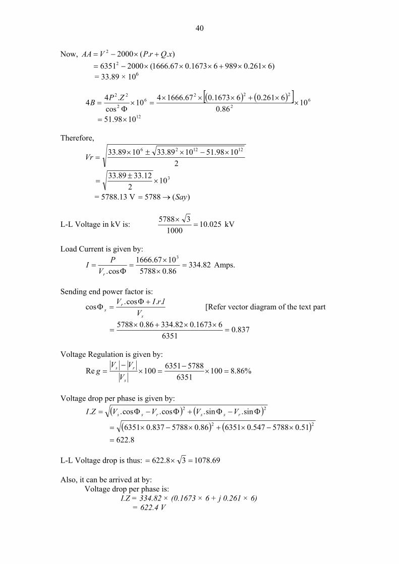
(a) Vector sum of I.Z drops of both halves of the line (b) Difference Sending end and Receiving end voltages

(a) 94.238019.15394.238119.153 jjVIZ +++= = 306.138 + j477.88 = 567.53 (Phase Voltage) = 982.96 (Line Voltage) (b) VoltageceivingVoltageSendingVdiff _Re_ −= = 5678 + j3719 – (5462 + j3239) = 306 + j480 = 567.52 (Phase Voltage) = 985.96 (Line Voltage) (The program has used second method i.e. (b) for calculations). NOTE: While going through the above calculations, it would have been observed

that results obtained have some fractional variation. This is due to the consideration of parameter values upto several number of digits after the decimal. However, the final values are correct upto the shown places of decimal.

46

VOLTAGE REGULATION & DROP WHEN SENDING END VOLTAGE IS KNOWN INPUT PARAMETERS:

Sl.No. Description INPUT Remarks 1 Sending end voltage in kV 11 2 Receiving end Load in kW 5000 3 Power factor of the load 0.86 4 Load factor of the system 0.6 5 Name of overhead line Conductor LYNX 6 Length of the overhead line in km 6 7 Equiv.spacing between conductors in mm 700 8 OHL Conductor temperature in °C 40

RESULT GENERATED BY THE PROGRAM:

S.N. Description Unit OUTPUT Remarks

1 Receiving end load shared by conductor path kW 5000

2 Receiving end voltage of the OHL kV 10.025 3 Sending end power factor Factor 0.8367 4 Percentage voltage regulation % 8.86 5 Voltage drop in the overhead line/ phase Volts 622.78 6 Annual energy losses in the overhead line kWh 1457247 7 Total line losses (Maxm.) kW 337.56 8 Total line losses (rms value) kW 166.35 9 Resistance/ conductor of the OHL at 40°C Ohms 1.0037

10 Inductive React./ conductor of the OHL. Ohms 1.566 11 Capacitive React./ conductor of the OHL. Ohms - 12 Capacitance/ conductor of the OHL. MFD 0.078 13 Form factor of the system. Factor 1.17 14 Line efficiency of the OHL system. % 93.68 15 Surge impedance of the OHL. Ohms 252.747 16 Current through conductor of the OHL Amps. 334.8 17 Disruptive critical voltage/ phase kV 72.2 18 Equivalent impedance/ phase of OHL Ohms 1.8601 19 Equivalent Cu cs area of conductor sq.mm. 110 20 Equivalent Al cs area of conductor sq.mm. 183 21 Current carrying capacity of conductor Amps. 360

47

REGULATION & DROP WHEN RECEIVING END VOLTAGE IS KNOWN INPUT PARAMETERS:

Sl.No. Description INPUT Remarks 1 Receiving end voltage in kV 11 2 Receiving end Load in kW 5000 3 Power factor of the load 0.86 4 Load factor of the system 0.6 5 Name of overhead line conductor LYNX 6 Length of the overhead line in km 6 7 Equiv.spacing between conductors in mm 700 8 OHL Conductor temperature in °C 40

RESULT GENERATED BY THE PROGRAM:

S.N.

Description

Unit

OUTPUT

Remarks

1

Receiving end load shared by conductor path kW 5000

2 Sending end voltage of the OHL (L-L) kV 11.887 3 Sending end current/ phase of the OHL Amps. 305.07 4 Sending end power factor of the OHL Factor 0.8407 5 Percentage voltage regulation of the line % 7.46 6 Annual energy losses in the overhead line kWh 1210114 7 Total line losses (maximum in eq. kW) kW 280.32 8 Total line losses (rms value in eq. kW) kW 138.14 9 Resistance/ conductor of the OHL at 40°C Ohms 1.0037

10 Inductive React./ conductor of the OHL Ohms 1.566 11 Line efficiency of the OHL system. % 94.69 12 Receiving end current/ phase of the OHL Amps. 305.15 13 Form factor of the system. Factor 1.17 14 Total Capacitance/ phase of the OHL MFD 0.078 15 Receiving end capacitor current Amps. 0.026 16 Overhead line mid point capacitor current Amps. 0.108 17 Sending end capacitor current Amps. 0.026 18 Disruptive critical voltage/ phase kV 72.2 19 Equivalent impedance/ phase of OHL Ohms 1.8601 20 Equivalent Cu cs area of conductor sq.mm. 110 21 Equivalent Al cs area of conductor sq.mm. 183 22 Current carrying capacity of conductor Amps. 360 23 Capacitive React./ conductor of the OHL k.Ohms 40.8 24 Voltage DROP per phase in the OHL Volts 567.5

48

SELECTION OF MOST ECONOMICAL OVERHEAD LINE CONDUCTOR (SAMPLE CALCULATION)

GIVEN: Limiting size of OHL conductor is LYNX, system voltage is 11kV, inflated value of conductor constant K0 is 2150, length of OHL is 6km, loading capacity is 5000kW at 0.86 load power factor, conductor temperature is 40°C, annual interest and depreciation is 18%, span of OHL is 90m, annual load factor is 0.6, cost of unit energy is Rs. 2.30 and permissible voltage regulation is 9%. TO FIND: Most suitable OHL, receiving end voltage, sending end power factor, voltage regulation, voltage drop, rms line losses, corona loss, annual energy loss, resistance, reactance and capacitance per phase of the line, selected conductor on the basis of load current, most economical conductor and its cross sectional area, sag of OHL, recommended spacing of conductors, standard capacity of OHL in kWkm at 40°C and cost of OHL per km. From Tables for LYNX conductor: Resistance of the conductor/ phase at 20°C = 0.1554 Ω km/ Reactance of the conductor/ phase x = 0.261 km/Ω Resistance at 40°C is given by:

1673.05.261405.2411554.0 =

+×=r Ω km/

Now, 277.051.0261.086.01673.0sincos =×+×=Φ+Φ xr From the initial given values and assuming percentage regulation as 6% at 11kV, number of parallel circuits may be estimated by the following:

22540277.0

100006.086.011sincos

100 22

=×××

=Φ+Φ

×××=

xrrgpfkVkWkm

Number of parallel paths 233.122540

65000⇒=

×=

×kWkm

kmkW

Power to be transmitted per circuit kWcktkW 2500

25000

===

From the Form factor curve, FF=1.17 corresponding to LF=0.6

Load current AmpsVkWI m 2.305

86.01135000

cos3=

××Φ=

RMS current AmpsFFLFII mrms 22.21417.16.02.305 =××=××=

49

A. SELECTION ON THE BASIS OF ECONOMICAL CONDITIONS: Most economical cross sectional area of the OHL conductor is given by (Refer text part of this Software):

cktidK

TRFcktI

csa rms

×××

×=0

100665.21 mm2

Where TRF is cost of unit energy K0 is area cost index (refer text) Id is percentage rate of interest & depreciation

237.1262182150

3.21002

214665.21 mmcsa =××

××=

From Tables, it may be inferred that TWO circuits of LYNX conductor are not capable to reach the desired capacity. Hence, THREE circuits are taken and find the economical cross sectional area as under:

278.683182150

3.21003

214665.21 mmcsa =××

××=

From Tables, we find that THREE circuits of TIGER conductor are sufficient to carry the desired load under the most economical condition. B. SELECTION ON THE BASIS OF CURRENT CAPACITY: Taking a de-rating factor corresponding to 33.3% de-rated capacity of the OHL, the current for selection of conductor ids given by:

AcktI

I ms 16.244

22.3056.16.1 =

×=×=

From the Tables, it can be inferred that TWO nos. of TIGER conductors are capable to carry the given load. FINAL SELECTION AND VALUES: Finally we find in this case, logically, THREE circuits with TIGER conductor suitable to carry the given load under the given conditions. Now, Phase voltage is given by:

63513

1110003

1000=

×=

×=

kVkVp V

50

From Tables, we find for ACSR TIGER conductor: r = 0.2221, x = 0.282, conductor radius rd = 8.26, dead weight of conductor/km = 604 kg and tensile strength = 5758

Load per circuit = kWcktkW 67.1666

35000

==

Resistance at 40°C Ω=+

×= 2391.05.261405.2412221.0r

For a 6.0km long line r = 6 × 0.2391 = 1.4345 and x = 6 × 0.282 = 1.692

Active power per phase 5566.5553

67.16663/

⇒===circuitLoadkWP

Reactive power per phase 32986.0

51.0556cos

sin≈

×=

ΦΦ×

=kWPkWQ

Referring to text: ( )xkWQrctkWPkVAA p ×+××−= 20002

6351= ( )692.13294345.155620002 ×+××− 37= 610625. ×

And, ( )2

222610PF

xrkWPB +××=

( )

12

2

2226

10056.286.0

692.14345.155610

×=

+××=

Hence, 121023.84 ×=B

Now, ( ) 61222 10515.371023.8625.374 ×=×−=−= BAAE

And 661 1057.3710

2515.37625.37

2×=×

+=

+=

EAAEr

Therefore, receiving end voltage Er is: VEE rr 61291057.37 6

1 =×== => 10.615kV (L-L)

51

Sending end power factor is given by:

p

rr

s kV

rE

kWPE ×

Φ

×+Φ

cos1000cos

PF =

8538.06351

4345.086.06129

556100086.06129

=

×

××

+×=

Losses (rms) is given by:

1000

32 r

cktI

ckt rms ×

×=LL kW

83.6510004345.1

32143

2

=×

××3= kW

Effective weight of Conductor: Weight due to air thrust, assuming 33.7 kg/m² as the air pressure:

1000

27.331 lrdW ×××= kg/m

mkg /5567.0

1000126.827.

=

×××= 33

Dead weight of conductor (from Tables) W2 = 0.604 kg/m Effective weight of conductor:

mkgWW /8214.0604.0557.0 2222

21 =+=+W =

Taking factor of safety 2 (as per IER-1956), the OHL conductor tension is:

kgStrengthTensileUltimate 28792

57582

__===T

Maximum Sag of overhead line is given by:

mmmT

WL 7.28828798

90821.08

22

=×

×=

×=Sag

52

Spacing between conductors is given by:

+×=

15026.1 kVSGSPC m

mm4.769150112887.0 =

+×1260=

Capacitance per is given by:

F

rdSP

l µ0735.0

26.8769ln18

6

ln18=

×

=

×

=C

Disruptive Critical Voltage is given by:

100ln302.17 ×

××=

rdSPrdcV

kV

V8.64

7.64792

10026.8

769ln26.8302.17

==

×

××=

Total Energy Loss in the OHL is: LLW=LL × 8760 = 65.83 × 8760 = 575444.4 kWh Line Efficiency is given by:

%7.98100

3383.65556

556

3

=×

×+

=

×+

=

cktLLkWP

kWPη

Voltage Regulation is given by:

4955.31006351

61296351100Re =×−

=×−

=p

rp

kVEkV

g

MWkm capacity of the line is given by:

Φ+Φ

×Φ=

sincoscos2

xrRGVMWkm

Here, V = 11, cos = 0.86, RG = 0.09 for 11kV, Φ r = 0.2391 at 40°C, x = 0.282

53

8007.26349446.0

09.086.0112

=××

=MWkm

Cost of overhead line per km is given by:

KK

KareaCondKt 0110 _ ×+×=cos (Please refer text

Where K0 = Value of index as on date K11 = Constant of the program (takes by default) K = Base value of area index (takes by default)

20302150316000802150cos ×+×=t for single circuit with TIGER

506680= Cost of Selected OHL per km is given by:

××+××=

2_cos 0

110cktInt

KK

KcktareaCondKt

1185360

2203021503160003802150

23

203021503160003802150

=

××+××=

××+××= Int

(Rs. Eleven lakhs eightyfive thousand and sixty) CABLE SELECTION (SAMPLE CALCULATION) GIVEN: Limiting size of cable is 240 mm², receiving end voltage is 3.3kV, percentage regulation should be limited to 9%, cable conductor temperature is 40°C, annual load factor is 0.6, conductor material is copper, cable length is 300m, load at the receiving end is 300kW at 0.86 power factor. Symm. Short circuit current is 5kA and breaking time of switchgear is 0.75 sec. Thermal admissibility constant for Cu is 116.8 Amp/mm². TO FIND: Most suitable cable, load current, regulation, sending end voltage, voltage drop, maximum and rms losses in the cable, resistance, reactance and capacitance per phase, cable selected on the basis of rms current, cable selected on the basis of regulation, cable selected on the basis of fault current, line efficiency, rms current, sending end power factor, dielectric loss, sheath loss and annual energy loss in the selected cable.

54

A. CABLE SELECTION BASED ON RMS CURRENT:

Load current AV

PIm 03.6186.03.33

300cos..3

=××

=Φ

=

Average current AFFI

I mav 16.52

17.103.61

===

RMS Current Irms = Im × LF × FF = 61.03 × 0.6 × 1.17 = 42.84 A Selection current Is = 2 × Irms = 2 × 42.84 = 85.68 A => 1 × 25 mm² Copper B. CABLE SELECTION BASED ON VOLTAGE REGULATION: Regulation has been set not to exceed 9%. Take the case of cable selected by the program and check for its suitability: For the selected one number of 2.5mm² copper cable: r/ km = 7.118 x/ km = 0.204 At 40°C the resistance and reactance of 300m long cable will be:

Ω=++

××= 2987.2205.241405.2413.0118.7r

x = 0.204 0215 0.3 = 0.0612 and, Ω C = 0.18 × 0.3 = 0.054 Fµ Voltage drop is given by: ( ) ([ ]Φ−Φ+Φ+Φ= sincossincosˆ. rxjxrIZI )

) =

( ) ([ ]

)(32.140336.68554.122

51.02987.286.00612.051.00612.086.02987.203.61

Absolutej

j

=−

×−×+×+××=

Sending end voltage is given by: V ZIVrs

ˆ.ˆˆˆ +=

( )

)(95.2028336.68554.122

336.68556.1220256.1905

Absolutej

jj

=−=

−++=

Regulation is given by:

%10.695.2028

256.190595.2028Re =−

=−

=s

rs

VVV

g

55

It will be observed that regulation is more than 9% in case we consider 1.5 mm² copper cable. So the cable selected on the basis of regulation is one no. of 2.5 mm² copper. C. CABLE SELECTION BASED ON FAULT CURRENT: Consider the symmetrical 3-phase fault current as the basis of selection. The minimum cross sectional area of the cable is given by:

KtconsityadmissibilThermaltimeBreakAmpscurrentcktShort

_tan__sec_____08.1 ××

=a mm²

Where K = 116.80 Amp/mm² for copper conductor K = 77.80 Amp/mm² for aluminium conductor

204.408.116

75.0500008.108.1mm

KtI

a sc =××

=××

=

So, the selected cable on the basis of short circuit fault current is the nearest higher size cable i.e. 50 mm². Summarizing all the three cases dealt above:

By rms current : 1 × 25 mm² Cu cable By Voltage Regulation : 1 × 2.5 mm² Cu cable By fault current : 1 × 50 mm² Cu cable

So, the recommended cable will be the highest one i.e. one no. of 50 mm² Cu cable. FINAL VALUES: r/km = 0.378 x/km = 0.08 At 40°C the values for the recommended cable will be:

Ω=××= 1221.05.2615.2813.0378.0r

x = 0.08 × 0.3 = 0.024 Ω C= 0.46 × 0.3 = 0.138 Fµ Voltage drop is given by: ( ) ([ ]51.01221.086.0024.051.0024.086.01221.003.61ˆ. ×−×+×+××= jZI )

=

)(5933.7

541.21555.7Absolute

j−=

Sending end voltage is given by: V ( ) 541.2715550256.1905ˆ jjs −++=

56

= )(4.3312

)(41.1912541.241.1912

LLVAbsolute

j

−→⇒

−=

Regulation is now given by:

%3741.010041.1912

256.190541.1912100Re =×−

=×−

=s

rs

VVV

g

Now, 6834.3086.0cos =Φ→→=Φ

π180)00133.0tan(

00133.041.1912

541.2tan

1

1

×−=Φ

−=−

=Φ

Arc

= - 0.076 Sending end power factor angle: 6074.30076.06834.301 =−=Φ+Φ=Φ s

Or cos 8606.0=Φ s

LOSS COMPONENTS AND LOSSES IN THE SELECTED CABLE: Losses (rms) WattsrI rms 26.6721221.084.4233 22 =××=××= Losses (Max) WattsrI m 3.13641221.003.6133 22 =××=××= Dielectric Losses 3= 007.0502138.09053.13 22 ××××××= πωδCV = 3.3 Watts Sheath Loss is given by: )__(_%2 LossesdielectricrmsofLsheath +=

( )Watts51.13

3.326.67202.0=

+×=

57

Total RMS Losses is therefore: WattsLrms 07.68951.133.326.672 =++= And Total Losses (Maximum) is: WattsL 11.138151.133.33.1364max =++=

Line efficiency %54.99100381.1300

300100 =×+

=×+

=LossesOutput

Outputη

Annual Energy Loss in kWh units is given by: 8760__ ×= LossesRMSTotalLosses = 0.689 × 8760 = 6035.64 = 6036 kWh

So, the annual energy loss in the selected cable will be 6036 kWh only.

58

GENERATED RESULTS OF CABLE SELECTION INPUT DATA: Limiting standard Cable size in m² = 240 Receiving end voltage in kV(L-L) = 3.3 Permissible % voltage regulation (upto 60) = 9 Load at the receiving end in kW = 300 Power factor of the load = 0.86 Load factor of the cable = 0.6 Length of the cable in m = 300 Mention the type of cable (Al/Cu) = cu Maximum Cable conductor temp. in °C = 40 Symmetrical short circuit current in kA = 5 Break time of ckt. breaker in sec (0.2 - 1.2) = 0.75 OUTPUT RESULTS: Cable Selected on the basis of Fault Current = 1 Cable(s) of 50 sq.mm. Cable Selected on the basis of RMS Current = 1 Cable(s) of 25 sq.mm. Cable Selected on the basis of Volt. Reguln. = 1 Cable(s) of 2.5 sq.mm. Recommended Cable = 1 Cable(s) of 50 sq.mm. CALCULATED PARAMETERS OF THE RECOMMENDED CABLE Required number of the cable lengths in parallel = 1 Cross Sectional Area of the selected cable sq.mm. = 50.0 Percentage voltage regulation (%) = 0.374 Voltage drop in the cable/phase in Volts = 7.6 Annual energy loss in the selected cable in kWh = 6036 Percentage line efficiency of the cable (%) = 99.5 Resistance of the cable/phase/conductor in ohms = 0.1221 Ind. reactance of the cable/phase/conductor in ohms = 0.0240 Capacitance of each cable/phase in MFD = 0.1380 Total losses in the cable (Average)- kW component = 0.689 Total losses in the cable (Maximum)- kW component = 1.381 Total dielectric losses in the cable- Watt component = 3.3 Total sheath loss in the cable- Watt component = 13.5 Sending end power factor = 0.861 Sending end voltage (L-L) in kV = 3.312 Calculated RMS current based on LF & FF in Amperes = 42.8 Maximum load current in Amperes = 61.0 Generated from Elect 7.05

59

TABLE-1 COPPER CABLE PROPERTIES AT 20.0°C AND 50.0Hz FREQUENCY

Sl. No.

Cable CSA in

mm²

Current Cap. in Amps.

R per km in Ohms

Xl per km in Ohms

C per km in MFD

Xc per km in

k.Ohms

Impedance per km in

Ohms 1 1.5 17 11.77 0.214 0.165 19.2915 11.7719 2 2.5 24 7.118 0.204 0.18 17.6839 7.1209 3 4 30 4.596 0.17 0.2 15.9155 4.5991 4 6 39 2.942 0.125 0.22 14.4686 2.9447 5 10 52 1.693 0.105 0.25 12.7324 1.6963 6 16 66 1.149 0.095 0.28 11.3682 1.1529 7 25 90 0.6614 0.086 0.385 8.2678 0.667 8 35 110 0.5309 0.083 0.42 7.5788 0.5373 9 50 135 0.378 0.08 0.46 6.9198 0.3864

10 70 165 0.2441 0.074 0.5 6.3662 0.2551 11 95 200 0.1959 0.072 0.535 5.9497 0.2087 12 120 230 0.1483 0.07 0.565 5.6338 0.164 13 150 265 0.1254 0.069 0.595 5.3497 0.1431 14 185 305 0.1007 0.0681 0.625 5.093 0.1216 15 225 340 0.091 0.067 0.655 4.8597 0.113 16 240 355 0.0769 0.0665 0.665 4.7866 0.1017 17 300 400 0.0611 0.066 0.7 4.5473 0.0899 18 400 455 0.0424 0.065 0.745 4.2726 0.0776 19 500 530 0.03 0.064 0.825 3.8583 0.0707 20 625 600 0.02 0.063 0.875 3.6378 0.0661

TABLE-2

ALUMINUM CABLE PROPERTIES AT 20.0°C AND 50.0Hz FREQUENCY

Sl. No.

Cable CSA in

mm²

Current Cap. in Amps.

R per km in Ohms

Xl per km in Ohms

C per km in MFD

Xc per km in

k.Ohms

Impedance per km in

Ohms 1 1.5 13 19.41 0.13 0.165 19.2915 19.4104 2 2.5 18 11.75 0.125 0.18 17.6839 11.7507 3 4 23 7.585 0.123 0.2 15.9155 7.586 4 6 30 4.854 0.121 0.22 14.4686 4.8555 5 10 40 3.019 0.118 0.25 12.7324 3.0213 6 16 51 1.914 0.115 0.28 11.3682 1.9175 7 25 70 1.102 0.113 0.385 8.2678 1.1078 8 35 86 0.8849 0.11 0.42 7.5788 0.8917 9 50 105 0.6299 0.104 0.46 6.9198 0.6384

10 70 130 0.4068 0.097 0.5 6.3662 0.4182 11 95 155 0.3265 0.097 0.535 5.9497 0.3406 12 120 180 0.2471 0.0941 0.565 5.6338 0.2644 13 150 205 0.209 0.091 0.595 5.3497 0.228 14 185 240 0.1678 0.0901 0.625 5.093 0.1905 15 225 270 0.1337 0.088 0.655 4.8597 0.1601 16 240 280 0.1165 0.086 0.665 4.7866 0.1448 17 300 315 0.1018 0.086 0.7 4.5473 0.1333 18 400 375 0.0707 0.083 0.745 4.2726 0.109 19 500 430 0.0583 0.0791 0.825 3.8583 0.0983 20 625 480 0.0509 0.077 0.875 3.6378 0.0923

60 DEFAULT DATA OF ACSR CONDUCTORS TABLE-3

S.N. Conductor Eq. Cu mm²

Eq. Al mm²

CCC Amps

Dia. in

mm

r/km ohm

xl/km ohm

Wt/km (kg)

UTS in kg Remarks

1 SQUIRREL 13 21 75 6.33 1.374 0.355 85 756 2 GOPHER 16 26 80 7.08 1.09 0.349 106 952 3 WEASEL 20 31 94 7.78 0.912 0.345 128 1106 4 FERRET 25 42 136 9 0.672 0.339 171 1503 5 RABBIT 30 52 156 10.05 0.545 0.335 214 1813 6 MINK 40 62 167 10.98 0.457 0.333 255 2207 7 BEAVER 45 73 186 11.98 0.391 0.33 303 2613 8 RACOON 48 78 204 12.27 0.366 0.329 319 2675 9 CAT 55 95 226 13.56 0.315 0.327 385 2982 10 DOG 65 105 240 14.15 0.275 0.315 394 3215 11 TIGER 80 128 295 16.52 0.222 0.282 604 5790 12 WOLF 95 154 335 18.13 0.184 0.266 726 6720 13 LYNX 110 183 360 19.54 0.155 0.261 844 7950 14 PANTHER 130 207 400 21 0.138 0.256 974 8934 15 LION 140 233 430 22.26 0.122 0.252 1097 10210 16 BEAR 160 258 470 23.46 0.11 0.25 1217 11310 17 GOAT 185 317 525 25.96 0.09 0.244 1492 13780 18 SHEEP 225 366 550 27.94 0.078 0.24 1726 15910 19 DEER 260 419 630 29.9 0.068 0.237 1977 18230 20 ELK 300 477 670 31.5 0.061 0.235 2196 20240

CALCULATED DATA OF ACSR CONDUCTORS TABLE-4 S.N. Conductor Eq. Cu

mm² Eq. Al mm²

CCC Amps

Dia. in mm

r/km ohm

xl/km ohm

Wt/km (kg)

UTS in kg Remarks

1 SQUIRREL 13 22 74 6.33 1.326 0.3549 85 741 2 GOPHER 16 27 85 7.08 1.06 0.3479 106 927 3 WEASEL 20 33 97 7.77 0.88 0.3421 128 1117 4 FERRET 25 44 119 9 0.656 0.3328 172 1499 5 RABBIT 30 55 141 10.05 0.526 0.3259 214 1869 6 MINK 40 65 163 10.98 0.441 0.3203 256 2230 7 BEAVER 45 77 188 11.97 0.371 0.3149 304 2651 8 RACOON 48 81 196 12.27 0.353 0.3133 319 2785 9 CAT 55 98 231 13.5 0.292 0.3073 386 3372 10 DOG 65 108 249 14.16 0.267 0.3043 394 3303 11 TIGER 80 137 288 16.52 0.209 0.2947 600 5809 12 WOLF 95 165 320 18.13 0.174 0.2888 723 6997 13 LYNX 110 192 350 19.53 0.15 0.2841 838 8119 14 PANTHER 130 222 385 21 0.13 0.2796 969 9387 15 LION 140 249 416 22.26 0.115 0.2759 1089 10547 16 BEAR 160 276 448 23.45 0.104 0.2726 1209 11705 17 GOAT 185 339 520 25.97 0.085 0.2662 1483 14356 18 SHEEP 225 392 581 27.93 0.073 0.2617 1715 16605 19 DEER 260 449 646 29.89 0.064 0.2574 1964 19017 20 ELK 300 498 703 31.5 0.058 0.2541 2181 21121

61 DEFAULT DATA OF AAAC CONDUCTORS TABLE-5

S.N. Conductor Eq. Cu mm²

Eq. Al mm²

CCC Amps

Dia. in mm

r/km ohm

xl/km ohm

Wt/km (kg)

UTS in kg Remarks

1 AAAC7/2.00 14 22 103 6 1.541 0.3583 60 657 2 AAAC7/2.50 21 34 137 7.5 0.99 0.3443 94 1031 3 AAAC7/315 34 55 188 9.45 0.621 0.3298 149 1634 4 AAAC7/381 50 80 240 11.43 0.425 0.3178 218 2386 5 AAAC7/426 63 100 278 12.78 0.339 0.3108 273 2983 6 AAAC19/289 78 125 321 14.45 0.274 0.3031 343 3735 7 AAAC19/315 93 148 359 15.75 0.229 0.2977 407 4434 8 AAAC19/340 108 173 397 17 0.197 0.2929 474 5152 9 AAAC19/366 125 200 437 18.3 0.171 0.2882 549 5980 10 AAAC19/394 145 232 481 19.7 0.147 0.2836 637 6937 11 AAAC37/315 180 288 554 22.05 0.118 0.2765 794 8635 12 AAAC37/345 216 346 624 24.15 0.098 0.2708 953 10355 13 AAAC37/371 250 400 687 25.97 0.083 0.2662 1102 11967 14 AAAC37/400 291 465 757 28 0.073 0.2615 1281 13902 15 AAAC61/331 328 525 820 29.79 0.065 0.2576 1448 14886 16 AAAC61/345 356 570 865 31.05 0.06 0.255 1574 16173 17 AAAC61/355 378 604 899 31.95 0.057 0.2532 1666 17124 18 AAAC61/366 401 642 935 32.94 0.053 0.2513 1771 18189 19 AAAC61/381 434 695 985 34.29 0.049 0.2488 1919 19699 20 AAAC61/400 479 767 1050 36 0.045 0.2457 2116 21714

CALCULATED DATA OF AAAC CONDUCTORS TABLE-6 S.N. Conductor Eq. Cu

mm² Eq. Al mm²

CCC Amps

Dia. in mm

r/km ohm

xl/km ohm

Wt/km (kg)

UTS in kg Remarks

1 AAAC7/2.00 14 22 106 6 1.547 0.3583 60 658 2 AAAC7/2.50 21 34 135 7.5 0.99 0.3443 94 1029 3 AAAC7/315 34 55 182 9.45 0.624 0.3298 149 1633 4 AAAC7/381 50 80 241 11.43 0.426 0.3178 219 2389 5 AAAC7/426 63 100 288 12.78 0.341 0.3108 273 2987 6 AAAC19/289 78 125 337 14.45 0.273 0.3031 341 3732 7 AAAC19/315 93 148 368 15.75 0.23 0.2977 406 4433 8 AAAC19/340 108 173 401 17 0.197 0.2929 473 5165 9 AAAC19/366 125 200 438 18.3 0.17 0.2882 548 5985 10 AAAC19/394 145 232 480 19.7 0.147 0.2836 635 6936 11 AAAC37/315 180 288 580 22.05 0.118 0.2765 790 8633 12 AAAC37/345 216 346 632 24.15 0.098 0.2708 948 10356 13 AAAC37/371 250 400 681 25.97 0.085 0.2662 1096 11975 14 AAAC37/400 291 465 740 28 0.073 0.2615 1274 13921 15 AAAC61/331 328 525 823 29.79 0.065 0.2576 1438 15715 16 AAAC61/345 356 570 858 31.05 0.06 0.255 1562 17073 17 AAAC61/355 378 604 883 31.95 0.056 0.2532 1654 18077 18 AAAC61/366 401 642 912 32.94 0.053 0.2513 1758 19215 19 AAAC61/381 434 695 953 34.29 0.049 0.2488 1906 20822 20 AAAC61/400 479 767 1008 36 0.044 0.2457 2100 22950

62 USER DATA OF AAC CONDUCTORS TABLE-7

S.N. Conductor Eq. Cu mm²

Eq. Al mm²

CCC Amps

Dia. in mm

r/km ohm

xl/km ohm

Wt/km (kg)

UTS in kg Remarks

1 Conops 13 21 100 6.454 1.359 0.3537 58 363 2 Gnat 16 26 116 6.63 1.09 0.352 72 444 3 Weevil 20 31 129 7.874 0.913 0.3412 86 521 4 LadyBird 25 42 159 8.37 0.672 0.3374 117 737 5 Ant 30 52 182 9.3 0.544 0.3308 144 892 6 Fly 40 63 207 10.198 0.453 0.325 174 1051 7 BlueBottle 45 73 225 10.978 0.391 0.3203 201 1203 8 GrassHopper 50 83 250 11.728 0.344 0.3162 230 1356 9 Cleg 60 95 270 12.508 0.301 0.3121 261 1523 10 Wasp 65 105 292 13.168 0.272 0.3089 290 1673 11 AAC 11 80 132 335 14.79 0.215 0.3016 369 2228 12 Peony 95 149 363 15.676 0.192 0.298 414 2484 13 Caterpillar 110 183 420 17.402 0.156 0.2914 511 2985 14 Chafer 130 210 460 18.636 0.136 0.2871 586 3381 15 AAC 15 140 234 495 19.67 0.122 0.2837 652 3736 16 AAC 16 160 262 530 20.802 0.109 0.2802 730 4144 17 AAC 17 185 318 600 22.92 0.09 0.2741 886 4947 18 AAC 18 225 367 654 24.65 0.078 0.2695 1025 5695 19 AAC 19 300 474 764 27.994 0.06 0.2615 1343 7289 20 Scorpion 325 518 805 29.288 0.055 0.2587 1464 7878

USER DATA OF ACSR CONDUCTORS TABLE-8

S.N. Conductor Eq. Cu mm²

Eq. Al mm²

CCC Amps

Dia. in mm

r/km ohm

xl/km ohm

Wt/km (kg)

UTS in kg Remarks

1 Squirrel 13 21 75 6.32 1.374 0.355 85 771 2 Gopher 16 26 80 7.08 1.09 0.349 106 952 3 Weasel 20 31 94 7.78 0.917 0.345 125 1136 4 Ferret 25 42 136 9 0.672 0.339 171 1503 5 Rabbit 30 52 156 10.06 0.545 0.335 214 1860 6 Mink 40 62 167 10.98 0.457 0.333 255 2207 7 Beaver 45 73 186 11.98 0.391 0.33 303 2613 8 Racoon 48 78 204 12.28 0.366 0.329 318 2746 9 Cat 55 95 226 13.56 0.315 0.327 385 3324 10 Dog 65 104 240 14.16 0.275 0.315 394 3899 11 Tiger 80 128 295 16.52 0.222 0.282 604 5790 12 Wolf 95 154 335 18.14 0.184 0.266 727 7350 13 Lynx 110 183 360 19.54 0.155 0.261 844 7950 14 Panther 130 207 400 21 0.138 0.256 976 9127 15 Lion 140 233 430 22.26 0.122 0.252 1097 10210 16 Bear 160 258 470 23.46 0.11 0.25 1217 11310 17 Goat 185 317 525 25.96 0.09 0.244 1492 13780 18 Sheep 225 336 550 27.94 0.077 0.24 1726 15910 19 Deer 260 419 630 29.9 0.068 0.237 1977 18230 20 Elk 300 477 670 31.5 0.061 0.235 2196 20240

63 PHYSICAL COSTANTS OF CALCULATING ACSR DATA TABLE - 9

SL.NO. C O N S T A N T S VALUE

1 Specific gravity of Aluminium 2.703 2 Specific gravity of Steel 7.85 3 Ultimate Tensile strength of Aluminium in kg/mm² 13 4 Ultimate Tensile strength of Al Alloy in kg/mm² 29.9 5 Ultimate Tensile strength of Steel in kg/mm² 143 6 Electrical Resistivity of Copper ohm mm²/km 17.86 7 Electrical Resistivity of Aluminium ohm mm²/km 28.7 8 Electrical Resistivity of Steel ohm mm²/km 150 9 Permittivity of free space 8.8x10^(-12)

10 Normal Temperature in °C 20 11 Equiv.spacing between conductors in mm 700

PHYSICAL COSTANTS OF CALCULATING AAAC DATA TABLE - 10 SL.NO. C O N S T A N T S VALUE

1 Specific gravity of Aluminium 2.703 2 Specific gravity of Steel 7.85 3 Ultimate Tensile strength of Aluminium in kg/mm² 13 4 Ultimate Tensile strength of Al Alloy in kg/mm² 29.9 5 Ultimate Tensile strength of Steel in kg/mm² 143 6 Electrical Resistivity of Copper ohm mm²/km 17.86 7 Electrical Resistivity of Aluminium ohm mm²/km 28.7 8 Electrical Resistivity of Steel ohm mm²/km 150 9 Permittivity of free space 8.8x10^(-12)

10 Normal Temperature in °C 20 11 Equiv.spacing between conductors in mm 700

SofexIndia

64

COSTING OF 3-PHASE POWER CABLES

A series of cost of different voltage grades, insulations, conductors etc. are collected from

various reliable sources and the prevailing market on a base date of September 2003. The

following categories are then constituted for group generalization:

1. Voltage (650/1100, 3300, 6600, 11000 and 33000V)

2. Conductor (Copper and Aluminium)

3. Armouring (Armoured and Unarmoured)

4. Number of Cores (3, 3½ and 4)

5. Insulation (PVC, XLPE and PILC)

Based on the data collected the following graphs were drawn between cross sectional area

(csa) in sq.mm. and unit cost of cable in Rs. ‘000. The graphs are enclosed with this text for

ready reference:

A. 1100V, Al, Unarmoured, 3-Core and PVC insulation cables

B. 1100V, Al, Armoured, 3-Core and PVC insulation cables

C. 3300V, Al, Armoured, 3-Core and PVC insulation cables

D. 3300V, Al, Armoured, 3-Core and XLPE insulation cables

E. 3300V, Cu, Armoured, 3-Core and PVC insulation cables

F. 3300V, Al, Armoured, 3-Core and PILC insulation cables

G. 6600V, Al, Armoured, 3-Core and XLPE insulation cables

H. 6600V, Al, Armoured, 3-Core and PILC insulation cables

I. 6600V, Cu, Armoured, 3-Core and PVC insulation cables

J. 11000V, Al, Armoured, 3-Core and PVC insulation cables

K. 11000V, Al, Armoured, 3-Core and XLPE insulation cables

L. 11000V, Al, Armoured, 3-Core and PILC insulation cables

M. 11000V, Cu, Armoured, 3-Core and PVC insulation cables

N. 33000V, Al, Armoured, 3-Core and XLPE insulation cables

The trends of variation of costs with the cross sectional areas, csa, of cable/km are then

obtained and are shown in the following table:

65

Sl. No.

Voltage Grade Core Arm-

ouring Cond- uctor Insulation Trend Equation Basis

A

1100 3 U Al PVC 2242.1 +×= acpkm PMP

B

1100 3 A Al PVC 3545.1 +×= acpkm PMP

C

3300 3 A Al PVC 7595.2 +×= acpkm PMP

D

3300 3 A Al XLPE 31582.3 +×= acpkm PMP

E

3300 3 A Cu PVC 8054.5 +×= acpkm PMP

F

3300 3 A Cu PILC Abnormal curve PMP

G

6600 3 A Al XLPE 33814.4 +×= acpkm PMP

H

6600 3 A Al PILC 33864.4 +×= acpkm PMP

I

6600 3 A Cu PVC 32036.7 +×= acpkm PMP

J

11000 3 A Al PVC 52432.4 +×= acpkm PMP

K

11000 3 A Al XLPE 52491.4 +×= acpkm PMP

L

11000 3 A Al PILC 59492.7 +×= acpkm PMP

M

11000 3 A Cu PVC Much deviated figures are obtained PMP

N

33000 3 A Al XLPE 10403875.5 +×= acpkm PMP

PMP – Prevailing Market Price A- Armoured U- Unarmoured Al- Aluminium Cu- Copper

66

To start with, we find the difference of cost between copper and aluminium conductors for a

three phase cable with different cross sections. The method by which this difference in cost

cd is obtained is given hereunder in the table:

COST DIFFERENCE BETWEEN Cu & Al

Cable CS

Area

Wt. of Al in kg

Wt. of Cu in kg Sl.

No. sq.mm.

VOLUME in litre

2.703 8.93

Cost of Al in Rs. '000

Cost of Cu in Rs. '000

Cost Diff. in

Rs. '000

1 1.5 4.5 12 40 1.5 8.0 6.6 2 2.5 7.5 20 67 2 13 11.0 3 4 12 32 107 4 21 18 4 6 18 49 161 6 32 26 5 10 30 81 268 10 54 44 6 16 48 130 429 16 86 70 7 25 75 203 670 24 134 110 8 35 105 284 938 34 188 153 9 50 150 405 1340 49 268 219

10 70 210 568 1875 68 375 307 11 95 285 770 2545 92 509 417 12 120 360 973 3215 117 643 526 13 150 450 1216 4019 146 804 658 14 185 555 1500 4956 180 991 811 15 225 675 1825 6028 219 1206 987 16 240 720 1946 6430 234 1286 1052 17 300 900 2433 8037 292 1607 1315 18 400 1200 3244 10716 389 2143 1754 19 500 1500 4055 13395 487 2679 2192 20 625 1875 5068 16744 608 3349 2741

67

EMPIRICAL FORMULAE FOR COSTING OF 3-CORE POWER CABLES Referring to foregoing equations, derived on the basis of the trend of prevailing market price as on 1st September 2003 and the difference of cost between copper and aluminium conductors, the following equations are set for the different types and category of power cables:

S. N.

Volt-age

Armo- uoring

Cores

Cond- uctor

Insul-ation Empirical Equation Basis

1 PVC PMP

2

Al

XLPE D

3 PVC D

4

U 3

Cu

XLPE D

5 PVC PMP

6

Al

XLPE D

7 PVC D

8

1100

A 3

Cu

XLPE D

9 PVC PMP

10 XLPE PMP

11

Al

PILC D

12 PVC PMP

13 XLPE D

14

3300 A 3

Cu

PILC D

15 PVC D

16 XLPE PMP

17

Al

PILC PMP

18 PVC PMP

19 XLPE D

20

6600 A 3

Cu

PILC D

21 11000 A 3 Al PVC PMP

a

a

×

a

a

+

+

2242.1 +×=cpkm

)2242.1(37.1 +××= acpkm

cdcpkm ++×= 2242.1

)2242.1(37.1 cdacpkm ++××=

3545.1 +×= acpkm

( )3545.137.1 +××= acpkm

cdacpkm ++×= 3545.1

( )cdacpkm ++××= 3545.137.1

7595.2 +×=cpkm

31582.3 += acpkm

31532.4 +×= acpkm

8054.5 +×=cpkm

cdacpkm ++×= 31582.3

cdacpkm ++×= 31532.4

cdacpkm −×= 32036.7

33814.4 +×= acpkm

33864.4 +×= acpkm

32036.7 +×= acpkm

cdacpkm +×= 33814.4

cdacpkm ++×= 33864.4

52432.4 +×= acpkm

68

S. N.

Volt-age

Armo- uoring

Cores

Cond- uctor

Insul-ation Empirical Equation Basis

22 XLPE PMP

23 PILC PMP

24 PVC D

25 XLPE D

26

Cu

PILC D

27 Al XLPE PMP

28

33000 A 3

Cu XLPE D

a

52491.4 +×= acpkm

59492.7 +×= acpkm

cdcpkm ++×= 52432.4

cdacpkm ++×= 52491.4

cdacpkm ++×= 59492.7

10403875.5 +×= acpkm

cdacpkm ++×= 10403875.5 Abbrv.: cd- Cost Difference (Cu-Al) cpkm– Cost/km in Rs. ‘000 a- csa in sq.mm. D- Derived POWER CABLES OF 3½ and 4-CORES The cost per km of cables of 3½ and 4 core cables of different voltages, conductors and insulations have been directly derived on the basis as under:

Cost of 3½ Core Cable = 1.10 x Cost of 3 Core Cable Cost of 4 Core Cable = 1.20 x Cost of 3 Core Cable

69

COSTING OF OVERHEAD LINES Overhead Line is not a single entity. Moreover, each entity of it has number of different values. So, costing of overhead lines has to consider a number of factors involved and affecting the present cost. In the following para, an effort has been made to arrive at a very close estimate for the cost of a given overhead line of any possible specification. The major entities of overhead lines are as under:

1. Working Voltage 2. Insulators 3. Type of Circuit 4. Type of Conductor 5. Conductor 6. Earth Conductor 7. Type of Structure & Heights 8. Earthing 9. Ruling Span 10. Date of estimate

1. WORKING VOLTAGE

The following working voltages have been considered in the cost estimation:

a. 415 V b. 550 V c. 3300 V d. 6600 V e. 11000 V f. 33000 V g. 132000 V h. 220000 V

2. INSULATORS

The following types of Insulators have been considered in the cost estimation:

a. Pin type LT Insulator b. Pin type HT Insulator c. 11000V Disc type Insulator

For 415V and 550V only Pin type LT Insulator has been considered in costing, while for 3300V and 6600V Pin type HT Insulator has been considered for costing. For 11000V and above only 11kV Disc type Insulators have been considered. Numbers of 11kV Insulators in series are taken as under:

a. 33000 V - Each string of 3x11000V b. 132000 V – Each string of 12x11000V c. 220000 V – Each string of 20x11000V

70

3. TYPE OF CIRCUIT

The following types of circuits have been considered in the cost estimation:

a. Single Circuit – Each phase having 1 conductor i.e. 3-Conductors b. Double Circuit - Each phase having 2 conductors i.e. 6-Conductors

4. TYPE OF CONDUCTOR

The following types of Conductors have been considered in the cost estimation:

a. ACSR Conductor (Aluminium Conductor Steel Reinforced) b. AAAC Conductor (All Aluminium Alloy Conductor)

It is to be noted that cost of conductor is proportional to volume or weight of Aluminium/ Steel. This may be inferred from above that cost of conductor is proportional to equivalent Aluminium cross sectional area of the types of conductors.

5. CONDUCTOR Series of 20 commonly used conductors in each type have been considered in the cost estimation. The list of each series is as under:

ACSR Eqv. Al Area in sq. mm.

AAAC Eqv. Al Area in sq. mm.

SQUIRREL 21 AAAC7/2.00 22 GOPHER 26 AAAC7/2.50 34 WEASEL 31 AAAC7/3.15 55 FERRET 42 AAAC7/3.81 80 RABBIT 52 AAAC7/4.26 100 MINK 62 AAAC19/2.89 125 BEAVER 73 AAAC19/3.15 148 RACOON 78 AAAC19/3.40 173 CAT 95 AAAC19/3.66 200 DOG 105 AAAC19/3.94 232 TIGER 128 AAAC37/3.15 288 WOLF 154 AAAC37/3.45 346 LYNX 183 AAAC37/3.71 400 PANTHER 207 AAAC37/4.00 465 LION 233 AAAC61/3.31 525 BEAR 258 AAAC61/3.45 570 GOAT 317 AAAC61/3.55 604 SHEEP 366 AAAC61/3.66 642 DEER 419 AAAC61/3.81 695 ELK 477 AAAC61/4.00 767

The names of the AAAC series indicate the diameter of the wire used in stranding of the conductor as per Indian Standards.

71

6. EARTH CONDUCTOR The following types of Earth Conductor of material Galvanized Steel Wire have been considered in the cost estimation:

1. 1x3.15 mm diameter – for 415V and 550V. 2. 7x2.59 mm diameter – for 3.3kV, 6.6kV and 11kV 3. 7x3.15 mm diameter – for 33kV 4. 7x3.55 mm diameter – 132kv and 220kV

7. TYPE OF STRUCTURES & THEIR HEIGHTS

The following types of structure for carrying the conductor and other accessories have been considered in the cost estimation:

a. Steel Tubular Poles (25kg/m) Hts: 8, 9, 10, 11, 12, 13 and 16m b. PCC Poles (400kg) Hts: 8(S), 9(S), 9.5(Virendeel), 9.5(S)m c. Rail Poles (52kg/m) Hts: 9, 9.5, 10, 11, 12, 13 and 15m d. Tower Structures Hts: 12m – 36m @ 3m Extension

8. EARTHING

The ELECT program has considered 2 earth points per km of overhead line.

9. RULING SPAN

Ruling Span has been defined at page no. 38 of the ‘Technology behind Elect’. The range of Ruling Span may be set any value between 5m and 500m.

10. DATE OF ESTIMATE This is again an important factor. Care has been taken for the overall cost escalation of overhead line. An average monthly escalation of 0.5% has been considered for this factor.

ESTIMATING INDIVIDUAL COSTS OF OHL ITEMS: Cost of overhead line shall be calculated on per km basis. For this, rates of various conductors, earth conductors, poles/ towers, insulators with hardware, clamps/ brackets are to be set as on a base date. This program has set base date as 1st September 2003. All basic rates are referred to that date. The different items whose costs are to be estimated are as under:

a. CONDUCTOR COST b. EARTH WIRE COST

72

c. STRUCTURE COST d. INSULATOR & HARDWARE COST e. BRACKETS/ CLAMPS ETC. COST f. PCC WORK AT POLES g. EARTHING COST h. TRANSPORATATION, ERECTION & SUPERVISION ETC.

a. CONDUCTOR COST Conductor cost Index has been set corresponding to the base date as:

Conductor Cost Index k = 2000 The use and method of finding this value of conductor cost index has been widely elaborated within the Elect program on the basis of the theory discussed at pages 12 to 15 of the ‘Technology behind Elect’. The conductor cost is given by: Cost = Index x Aluminium Area x No. of circuits x Escalation factor

Where Escalation factor = 1+ Rate Esc. x months passed b. EARTHWIRE COST The basic cost of 7x3.15 mm. GI wire is set at Rs. 25000/= per km. Cost of other combination of wires have been derived from this value as under i. 1x3.15 mm GI wire - 0.15 of Rs. 25000/= per km ii. 7x2.59 mm GI wire - 0.67 of Rs. 25000/= per km iii. 7x3.55 mm GI wire - 1.27 of Rs. 25000/= per km c. STRUCTURE COST Basic height-wise structure cost as on base date have been taken as under:

STEEL TUBULAR POLE

PCC POLE

RAIL POLE TOWER Ht.

Index COST COST COST COST BASE in m 0 4500 1600 15000 60000 2.6x2.6 1 5400 3300 17000 80000 3.5x3.5 2 8200 3000 19000 100000 4.2x4.2 3 11600 3500 23000 120000 5x5 4 14800 - 27000 142000 5.5x5.8 5 17400 - 31000 162000 6.7x6.7 6 21000 - 39000 180000 7.5x7.5 7 - - - 205000 8.4x8.4 8 - - - 225000 9.3x9.3

73

Number of structures per km is arrived at with the help of selected ‘SPAN’ of the overhead line.

No. of Structures = 1000/ Span

Where 1000m is unit length of Overhead line and Span is Ruling Span in metres

It is to be noted that the above relation may not always yield a whole number. It is always better to estimate on a bit higher side than actual. In view of this, the above value of number of structures should be rounded off on the higher side, if obtained in fraction. d. INSULATOR & HARDWARE COST Basic costs of insulators are as under:

1. LT Pin type @ Rs. 110/= per piece 2. HT Pin type @ Rs. 250/= per piece 3. 11kV Disc type @ Rs. 400/= per piece 4. Hardware for Disc type @ Rs. 500/= per set

Empirical formulae for insulator costs are as under: For PIN Type Insulators: Unit Rate of Pin Insulator = Base Rate x Esc. Cost = Unit Rate x Insulators/km For DISC Type Insulators: Cost = (Insulators/km x Rate + No. of Strings x 3 x Circuits x Rate of HW) x Esc.

Where Esc = 1+ Rate of Escalation x months passed and

Insulators/km = No. of Spans x 3 x Circuits x (kV/11) for 11kV and above e. BRACKETS/ CLAMPS ETC. COST Cost of brackets, angles, clamps etc. depend on number of bracket sets and weight of structure. Weight of structure in turn depends on weight of pole/ tower, insulators and conductors. The program for costing of brackets has used the following empirical formula: Cost = Bracket sets x Cost of (Structure + Insulator + Conductor) x 0.0015

74

f. COST OF PCC WORK AT POLES/ TOWERS Cost of Cement Concrete Work depends on number of working points and weight of structure. Weight of structure in turn depends on weight of pole/ tower, insulators and conductors. The program for costing of PCC has used the following empirical formula:

Cost = Pole/km x Cost of (Structure + Insulator + Conductor) x 0.0025 g. EARTHING COST As already stated, 2 earth points have been envisaged per km of overhead line in this program. Cost of two earth pits at suitable pole/ tower legs are estimated as equal to 10% of the cost of earth conductor/km and is given by the empirical relation as under:

Cost = Cost of Earth Conductor x 0.125 h. TRANSPORATATION, ERECTION & SUPERVISION ETC. COST Transportation of structure and other materials, stringing of insulators, drawing of conductors, earth wires etc. along with supervision of the entire work is taken as 25% of the overall cost of all materials. COST OF OVERHEAD LINE: Summing up the above estimated values of different items of overhead line, including the supervision and installation charges, it may concluded as under: Cost of OHL = Conductor Cost + Earth wire Cost + Structure Cost

+ Insulators & Hardware Cost + Brackets/ Clamps etc. Cost + PCC Work Cost + Earthing Cost + Supervision/ Transportation/ Erection etc.

75

ENERGY AUDIT REPORT OF OVERHEAD LINE AND ITS MOST ECONOMICAL CONDUCTOR WORKS/ PROJECT: Test Project Report Date: 26/11/04 CASE STUDY: A 2.5 km long, 11 kV overhead line with ACSR 'LYNX' conductor having 183 mm² equivalent aluminium area, delivers power to a certain works having an electrical load of 2000 kW at 0.9 power factor. The equivalent spacing between overhead line conductors is 700 mm and its temperature is 55°C. The annual load factor of the works is 0.5. Generate report of this existing line suggesting Most Economical Conductor for the above system. Also generate information of the suggested line alongwith benefits over the existing one. Take cost of unit energy as Rupees 3.05, rate of maximum demand charge as Rupees 200 per kVA per month and conductor Area Index as 2030. ANALYSIS REPORT: The overhead line under examination is making an annual transmission loss of 63109 kWh of energy. This loss of energy is equivalent to Rupees 1.925 lakh(s) per annum at the rate of Rupees 3.05 per kWh energy charge. Voltage Regulation in the existing overhead line is 1.27 percent. This Regulation is OK as per Indian Electricity Rules. Loading capacity of the existing overhead line is 35.99 MWkm under the given peripheral conditions. Current through the overhead line is 118.1 ampere(s) for the given load of 2000 kW. Most Economical Conductor for the overhead line under the given boundary conditions is 2 circuit(s) of DOG conductor having cross sectional area of 105 mm² (Equivalent aluminium area) i.e. 65 mm² equivalent nominal copper area. The Most Economical Conductor will reduce the annual line losses from 63109 kWh to 54332 kWh leading to an annual saving of 8777 kWh. In monitory terms this saving is equivalent to Rupees 0.268 lakh(s) per annum. Equivalent loss part of kVA demand (rms) will reduce from 7.2 kVA (rms) to 6.2 kVA (rms). This reduction in kVA demand leads to a gain of 1 kVA. The loading capacity of the line increases accordingly within the same contract demand. Further this reduction in kVA is equivalent to a saving of Rupees 0.024 lakh(s) per annum at the rate of Rupees 200 per kVA of Maximum Demand per month. Gross monitory saving will be Rupees 0.292 lakh(s) per annum. One time investment on re-organization of 2.5 km overhead line will be Rupees 6.598 lakh(s) only towards the cost of conductors and its associated accessories. This

76

amount does not include the cost of existing conductors, which will be about Rupees 5.583 lakh(s) only, had it been new conductors. However, it is to be noted that this Re-organization scheme has considered the continuation of the services of the existing overhead line and its conductor. In the re-organized arrangement of Most Economical Conductor, the number of circuits/ parallel conductors/ bundled conductors per phase will be 2 and additional number of parallel overhead line structures (on rail poles) will be 0. Thus the additional cost of structures will be Rupees 0 lakh(s). Estimated cost of exclusively new overhead line(s) as suggested above, with the Most Economical Conductors will be approximately Rupees 5.799 lakh(s) per km. This estimation is based on the Conductor Index of 2030 and rail pole structure for the overhead line. Assuming the production losses due to the downtime of the overhead to be 25% of the additional investment in re-organization, the downtime losses come to Rupees0.254 lakh(s) only. The total cost of re-organization, comprising of investment on additional conductors & related accessories, investment on additional overhead line structures and downtime losses, comes to Rupees1.269 lakh(s). Loading capacity of the line with the most economical conductor will be 46.958 MWkm. Voltage Regulation in the new overhead line will be 0.98 percent. This Regulation is BETTER than that in the existing line and is OK as per Indian Electricity Rules. For more details, the following annexed result sheets, obtained from the computerized program, may be consulted: 1. RESULTS OF REGULATION & DROP WHEN SENDING VOLTAGE IS KNOWN 2. RESULTS OF MOST ECONOMICAL CONDUCTOR SELECTION Pay Back period of this re-organization scheme will be 4.35 years. RECOMMENDATION: IMPLEMENT THE FINDINGS Report generated by Elect 7.05

77

REGULATION AND VOLTAGE DROP IN SINGLE CONDUCTOR OHL (Vs GIVEN) INPUT DATA : 1. Sending end voltage in kV 11.000 2. Receiving end Load in kW 2000 3. Power factor of the load 0.900 4. Load factor of the system 0.500 5. Name of overhead line Conductor LYNX 6. Length of the overhead line in km 2.5 7. Equiv.spacing between conductors in mm 700 8. OHL Conductor temperature in °C 55.0 R e s u l t s : 1 Receiving end load shared by conductor path kW 2000.0 2 Receiving end voltage of the OHL kV 10.86 3 Sending end power factor Factor 0.8968 4 Percentage voltage regulation % 1.27 5 Voltage drop in the overhead line/ phase Volts 93.00 6 Annual energy losses in the overhead line kWh 63109 7 Total line losses (Maxm.) kW 18.44 8 Total line losses (rms value) kW 7.20 9 Resistance/ conductor of the OHL at 55°C Ohms 0.4405 10 Inductive React./ conductor of the OHL. Ohms 0.6525 11 Capacitive React./ conductor of the OHL. Ohms - 12 Capacitance/ conductor of the OHL. MFD 0.0325 13 Form factor of the system. Factor 1.25 14 Line efficiency of the OHL system. % 99.09 15 Surge impedance of the OHL. Ohms 252.747 16 Current through conductor of the OHL Amps. 118.1 17 Disruptive critical voltage/ phase kV 72.2 18 Equivalent impedance/ phase of OHL Ohms 0.7873 19 Equivalent Cu cs area of conductor sq.mm. 110 20 Equivalent Al cs area of conductor sq.mm. 183 21 Current carrying capacity of conductor Amps. 360

78

RESULTS OF MOST ECONOMICAL CONDUCTOR SELECTION INPUT DATA : 1. Limiting conductor size for the overhead line LION (140 mm²) 2. OHL system voltage in kV (Sending end) 11.000 3. Loading capacity of OHL in kW 2000.0 4. Power factor of the load on overhead line 0.900 5. Annual Load factor of the system 0.500 6. Length of the overhead line in km 2.5 7. Average span of the overhead line in m 120 8. Overhead line Conductor temperature in °C 55.0 9. Permissible voltage regulation in percent (%) 9.000 10. Inflated value of cond. area constant 2030.00 11. Annual interest+depr. of conductor cost in % 15.00 12. Cost of unit electricity in Rupees 3.050 R e s u l t s : 1 Most economical number of OHL feeder(s) 2 Circuit(s) 2 Most economical Conductor selected for the OHL DOG 65 mm² 3 Receiving end voltage of the OHL 10.893 kV 4 Sending end power factor of the OHL 0.8985 5 Percentage voltage regulation of OHL 0.98 % 6 Voltage drop in the overhead line/phase 64.56 Volts 7 Total overhead line losses (rms) 6.20 kW 8 Line efficiency of the OHL system 99.7 % 9 Current through the overhead line 116.6 Amps 10 Disruptive critical voltage/phase 62.2 kV 11 Total corona loss in the OH Line 0.000 kW 12 Annual energy loss in the OH Line 54332 kWh 13 Total resistance/ phase of the OH Line 0.778 Ohms 14 Total inductive reactance/ phase of OHL 0.788 Ohms 15 Total capacitance of the line/ phase of OHL 0.027 MFD 16 Maximum sag of the overhead line 693 mm 17 Recommended spacing between conductors 1141 mm 18 Standard capacity of the selected OHL/feeder 23479 kWkm/ 9% rg 19 Cost of selected OHL & conductor /km in Rupees 579900 per km 20 Most economical conductor's equiv. Cu cs area 65 mm², 2 x DOG 21 Least no. of circuits for the given regulation 1 x DOG 22 Cond. selected on the basis of max. load current 48 mm², 1xRACOON

79

CALCULATION RESULTS FOR SAG AND TENSION OF OVERHEAD LINE (Data executed on 26/11/04 at 9:23:18 PM) I N P U T D A T A : Name of OHL Conductor = WOLF Overall conductor dia. in mm. = 18.13 Cross sectional area in mm² A = 194.04 Weight of cond. in kg/m Wc = 0.726 Ultimate Tensile strength in kg UTS = 6720 Coefficient of linear exp./°C (alpha) å = 17.78 × 10^-6 Modulus of Elast.'Initial' kg/m² E = 6260 Mod. of Elasticity 'Final' kg/m² E = 8158 Normal Span of overhead line in m span = 225 Ruling Span of overhead line in m span = 200 Minimum temp. of conductor in °C = 5 Everyday temp of conductor in °C = 32 Maximum temp.of conductor in °C = 75 Wind pressure in kg/sq.m. = 151.3 Percentage Worst Limiting Tension = 70 % Initial Limiting Tension at no load = 35 % Final Limiting Tension at no load = 25 Thickness of ice layer in mm = 0 Specific gravity of ice = 0.9168 C A L C U L A T I O N S : TENSION EQUATION IN TERMS OF STRESS IS GIVEN BY: f² = [f-(K - å × (t2-t1) × E)] = Z0 × (Loading Factor)² Where Z0 = (span × Delta)² × E / 24 t2 = Cond. temperature correspondig to stress f t1 = Cond. temperature correspondig to stress f1 å = Coefficient of linear expansion of cond. material E = Modulus of Elasticity (Final) K = f1 - (span × Delta × Loading factor)² × E / (24 × f1²) f1 = Stress corresponding to temperature t1 GIVEN STARTING CONDITION: No Wind and 32°C Factor of Safety = 4.00 Tension T = UTS / FoS = 6720 / 4.00 = 1680 kg. Corresponding stress f1 = T/A = 1680 / (194.04 × 10^-6) = 8.658 × 10^6 kg/m²

80

Conductor density- Delta = Wc/A = 0.726 / [194.04 × 10^(-6)] = 3741 kg/cu.m. Wind load = Wind pressure × conductor dia. = 151.3 × 0.01813 = 2.7431 kg/m. Loading factor corresponding to No Wind

= Effective load on cond./ Conductor weight = Sqrt[(ZeroWind)² + (Weight_Cond)²] / (Weight_Cond) = Sqrt(0.² + 0.726²) / 0.726 = 1.0 Constant K = stress - (span × Delta × Loading factor)² × Mod. of Elas./ (24 × stress²) Or K = 8.658 × 10^6 - (200 × 3741 × 1.0)² × 8158 × 10^6 / ( 24 × 8.658² × 10^12) = 6.1189 × 10^6 Now Sag = EffectiveConductorLoad × span² / (8 × Tension) = Delta × LoadingFactor × span² / (8 × stress) = 3741 × 1.0 × 225 / (8 × 8.658 × 10^6) = 10.688 m (Deflected) Vertical Sag = Delta × NoWind_LoadingFactor × span² / (8 × stress) = 3741 × 1.0 × 225² / (8 × 8.658 × 10^6) = 2.735 m Swing from Vertical at Full Wind Load & 36% Wind Load: Angle of swing = Arctan (Wind load/ Dead wt. of conductor) Full load swing Angle = 75.2° 36% Wind load swing Angle = 53.7° Note: Values of Vertical & Horizontal components of Sags can be found using these angles suitably for different loading conditions. Values of K - å × (t2-t1) × E at 5°C, 32°C, 75°C respectively are: K - å × t × E = 6.1189 × 10^6 - 17.780 × 10^-6 × (5 - 32) × 8158 × 10^6 = 10.0352 × 10^6 K - å × t × E = 6.1189 × 10^6 - 17.780 × 10^-6 × (32 - 32) × 8158 × 10^6 = 6.1189 × 10^6 K - å × t × E = 6.1189 × 10^6 - 17.780 × 10^-6 × (75 - 32) × 8158 × 10^6 = -.1183 × 10^6 Value of Z0 is given by: Z0 = (200 × 3741)² × 8158 × 10^6 / 24 = 190.3370 × 10^18 VALUES OF Z, STRESS AND TENSION AT FULL WIND AND DIFFERENT TEMPS. Stress is found from the Tension equation by putting values of Z and K-å.(t2-t1).E

81

VALUES AT FULL WIND & 5°C: Z = Z0 × (Load factor)² = 190.3370 × 10^18 × 3.908² = 2907.5481 × 10^18 Solving the obtained equation for Stress/ Tension at 5°C: f² = [f- (10.0352 × 10^6 )] = 2907.5481 × 10^18 Stress (f) at Full Wind & 5°C = 18.5158 × 10^6 kg/m² (by iterative method) Tension at 5°C = Stress × Area = 18.5158 × 10^6 × 194.04 × 10^-6 = 3593 kg Sag at 5°C = Delta × Loading factor × span² / (8 × stress) = 3741 × 3.908 × 225² / (8 × 18.516 × 10^6) = 4.998 m VALUES AT FULL WIND & 32°C: Z = Z0 × (Load factor)² = 190.3370 × 10^18 × 3.908² = 2907.5481 × 10^18 Solving the obtained equation for Stress/ Tension at 32°C: f² = [f- (6.1189 × 10^6 )] = 2907.5481 × 10^18 Stress (f) at Full Wind & 32°C = 16.6308 × 10^6 kg/m² (by iterative method) Tension at 32°C = Stress × Area = 16.6308 × 10^6 × 194.04 × 10^-6 = 3227 kg Sag at 32°C = Delta × Loading factor × span² / (8 × stress) = 3741 × 3.908 × 225² / (8 × 16.631 × 10^6) = 5.564 m VALUES AT FULL WIND & 75°C: Z = Z0 × (Load factor)² = 190.3370 × 10^18 × 3.908² = 2907.5481 × 10^18 Solving the obtained equation for Stress/ Tension at 75°C: f² = [f- (-.1183 × 10^6 )] = 2907.5481 × 10^18 Stress (f) at Full Wind & 75°C = 14.2334 × 10^6 kg/m² (by iterative method) Tension at 75°C = Stress × Area = 14.2334 × 10^6 × 194.04 × 10^-6 = 2762 kg Sag at 75°C = Delta × Loading factor × span² / (8 × stress) = 3741 × 3.908 × 225² / (8 × 14.233 × 10^6) = 6.502 m VALUES OF Z, STRESS AND TENSION AT 36% WIND LOAD AND DIFFERENT TEMPS. VALUES AT 36% WIND LOAD & 5°C: Z = Z0 × (Load factor)² = 190.3370 × 10^18 × 1.688² = 542.4875 × 10^18

82

Solving the obtained equation for Stress/ Tension at 5°C: f² = [f- 10.0352 × 10^6 ] = 542.4875 × 10^18 Stress (f) at 36% Wind Load & 5°C = 13.1651 × 10^6 kg/m² (by iterative method) Tension at 5°C = Stress × Area = 13.1651 × 10^6 × 194.04 × 10^-6 = 2555 kg Sag at 5°C = Delta × Loading factor × span² / (8 × stress) = 3741 × 1.688 × 225² / (8 × 13.165 × 10^6) =3.036 m VALUES AT 36% WIND LOAD & 32°C: Z = Z0 × (Load factor)² = 190.3370 × 10^18 × 1.688² = 542.4875 × 10^18 Solving the obtained equation for Stress/ Tension at 32°C: f² = [f- 6.1189 × 10^6 ] = 542.4875 × 10^18 Stress (f) at 36% Wind Load & 32°C = 10.7837 × 10^6 kg/m² (by iterative method) Tension at 32°C = Stress × Area = 10.7837 × 10^6 × 194.04 × 10^-6 = 2092 kg Sag at 32°C = Delta × Loading factor × span² / (8 × stress) = 3741 × 1.688 × 225² / (8 × 10.784 × 10^6) =3.707 m VALUES AT 36% WIND LOAD & 75°C: Z = Z0 × (Load factor)² = 190.3370 × 10^18 × 1.688² = 542.4875 × 10^18 Solving the obtained equation for Stress/ Tension at 75°C: f² = [f- -.1183 × 10^6 ] = 542.4875 × 10^18 Stress (f) at 36% Wind Load & 75°C = 8.1164 × 10^6 kg/m² (by iterative method) Tension at 75°C = Stress × Area = 8.1164 × 10^6 × 194.04 × 10^-6 = 1575 kg Sag at 75°C = Delta × Loading factor × span² / (8 × stress) = 3741 × 1.688 × 225² / (8 × 8.116 × 10^6) =4.925 m VALUES OF Z, STRESS AND TENSION AT NO WIND LOAD AND DIFFERENT TEMPS. VALUES AT NO WIND LOAD & 5°C: Z = Z0 × (Load factor)² = 190.3370 × 10^18 × 1.0² = 190.3370 × 10^18 Solving the obtained equation for Stress/ Tension at 5°C: f² = [f- 10.0352 × 10^6 ] = 190.3370 × 10^18 Stress (f) at NO Wind Load & 5°C = 11.4794 × 10^6 kg/m² (by iterative method) Tension at 5°C = Stress × Area = 11.4794 × 10^6 × 194.04 × 10^-6 = 2227 kg

83

Sag at 5°C = Delta × Loading factor × span² / (8 × stress) = 3741 × 1.0 × 225² / (8 × 11.479 × 10^6) = 2.063 m VALUES AT NO WIND LOAD & 32°C: Z = Z0 × (Load factor)² = 190.3370 × 10^18 × 1.0² = 190.3370 × 10^18 Solving the obtained equation for Stress/ Tension at 32°C: f² = [f- 6.1189 × 10^6 ] = 190.3370 × 10^18 Stress (f) at NO Wind Load & 32°C = 8.6580 × 10^6 kg/m² (by iterative method) Tension at 32°C = Stress × Area = 8.6580 × 10^6 × 194.04 × 10^-6 = 1680 kg Sag at 32°C = Delta × Loading factor × span² / (8 × stress) = 3741 × 1.0 × 225² / (8 × 8.658 × 10^6) = 2.735 m VALUES AT NO WIND LOAD & 75°C: Z = Z0 × (Load factor)² = 190.3370 × 10^18 × 1.0² = 190.3370 × 10^18 Solving the obtained equation for Stress/ Tension at 75°C: f² = [f- -.1183 × 10^6 ] = 190.3370 × 10^18 Stress (f) at NO Wind Load & 75°C = 5.7131 × 10^6 kg/m² (by iterative method) Tension at 75°C = Stress × Area = 5.7131 × 10^6 × 194.04 × 10^-6 = 1109 kg Sag at 75°C = Delta × Loading factor × span² / (8 × stress) = 3741 × 1.0 × 225² / (8 × 5.713 × 10^6) = 4.144 m CHECKING PARAMETERS WITH INITIAL MODULUS OF ELASTICITY AT NO WIND LOAD AND EVERYDAY TEMPERATURE VALUES AT NO WIND LOAD & 32°C: Z = Z0 × (Load factor)² = 190.3370 × 10^18 × 1.0² × 6260 × 10^6 / (8158 × 10^6) = 146.0541 × 10^18 Solving the obtained equation for Stress/ Tension at 32°C: f² = [f- .0000 × 10^6 ] = 146.0541 × 10^18 Stress (f) at NO Wind Load & 32°C = 5.2663 × 10^6 kg/m² (by iterative method) Tension at 32°C = Stress × Area = 5.2663 × 10^6 × 194.04 × 10^-6 = 1022 kg Sag at 32°C = Delta × Loading factor × span² / (8 × stress) = 3741 × 1.0 × 225² / (8 × 5.266 × 10^6) = 4.496 m

84

CHECKING PARAMETERS WITH INITIAL MODULUS OF ELASTICITY AT FULL WIND LOAD AND EVERYDAY TEMPERATURE VALUES AT FULL WIND LOAD & 32°C: Z = Z0 × (Load Factor)² = 190.3370 × 10^18 × 3.908² × 6260 × 10^6 / (8158 × 10^6) = 2231.0923 × 10^18 Solving the obtained equation for Stress/ Tension at 32°C: f² = [f- .0000 × 10^6 ] = 2231.0923 × 10^18 Stress (f) at FULL Wind Load & 32°C = 13.0669 × 10^6 kg/m² (by iterative method) Tension at 32°C = Stress × Area = 13.0669 × 10^6 × 194.04 × 10^-6 = 2535 kg Sag at 32°C = Delta × Loading factor × span² / (8 × stress) = 3741 × 3.908 × 225² / (8 × 13.067 × 10^6) = 7.082 m Calculations generated by Elect 7.05 from SofexIndia CALCULATION RESULTS FOR ELECTRICITY BILL (Data executed on 26/11/04 at 9:27:47 PM) I N P U T D A T A : Power Supply Company = ComF Bill No. = 51040200050 Bill Cycle = January '2004 Payment made = Before due Date Due Date = 27/03/2004 Meter ID No. = BH-NJ-TVMSEMWBU02088 Voltage = 11000. Multiplic. Factor (kWh) = 6.00 Mult. Factor (MaxDem) = 6.00 Contract Demand kVA = 400 Maximum Demand kW = 214.00 Maximum Demand kVA = 350.00 Opening Reading = 10390.00 Closing Reading = 14805.00 Total Hours = 792.00 Interruption Hrs. = 2.98 Rebate Hours = 0.00 Domestic Units = 0 Industrial Units = 26490 Commercial units = 0 Exempted Units = 0

85

Ind. Duty Rate (%) = 7.50 Dom. Duty Rate (%) = 10.00 Enr.Tariff (Rs./Unit) = 3.0743 Intrm. Ch. (Re./Unit) = 0.06 Meter Rent = 1200.00 Avail compens. (%) = 1.00 Rebate/ kWh on Energy Charge for Timely Payment (paise) = 10 Penalty/ kWh on Energy Charge for Late Payment (paise) = 10 Rate of Surcharge for Late Payment/month or part (%) = 1.25 Penalty on shortfall of cons. below 20% LF (Paise/kWh) = 20 Rebate on excess cons./kWh above 80% LF in paise = 20 Rate of Penalty for Exceeding CD on Net Energy Bill (%) = 1 C A L C U L A T I O N S : (Note: Units & Amounts have been converted to long integer) kVA Contract Demand taken for calculations = 400 kVA Units consumed = Diff. in Open-Close readings × MF = (14805 - 10390) × 6 = 4415 × 6 = 26490 Power Factor = Maximum kW Demand/ Maximum kVA Demand = 214 / 350 = 0.61 Load Factor = Units consumed × 100 / ( CD × Available Hours × PF) = 26490 × 100 / [400 × (792.0 - 2.98) × 0.610] = 13.76 Energy Charges = Units consumed × Unit Energy Charge = 26490 × 3.0743 = 81438.00 Load Factor Penalty Charge for LF of 13.76 Panalty = Rate of penalty × CD × (20 - LF) × Available Hours × PF/100 = 0.20 × 400 × (20 - 13.76) × (792.0 - 2.98) × 0.610/100 = 2403.00 REBATE / PENALTY FOR TIME OF PAYMENT Since payment made is Before due Date Rate of rebate is = 0.1 Rabate for timely payment = Rebate Rate × Units Consumed = 0.1 × 26490 = 2649.00 TOTAL NET CHARGE: Net Energy Charge = Energy Ch. + LF Penalty - Pay Time Rebate = 81438.00 + 2403.00 - 2649.00 = 81192.00 INTERIM CHARGE INDUSTRIAL+COMMERCIAL+DOMESTIC: Interim Indusrial Energy Charge = Industrial Units × Rate = 26490 × 0.06

86

= 1589.00 Interim Domestic Energy Charge = Domestic Units × Rate = 0 × 0.06 = 0.00 Interim Commercial Energy Charge = Commercial Units × Rate = 0 × 0.06 = 0.00 TOTAL Interim Charges = 1589.00 + 0.00 + 0.00 = 1589.00 COMPENSATION FOR LOW AVAILABILTY OF POWER: Power Availability Factor = (Total Hours - Interruption) × 100/ Total Hours = (792 - 2.98) × 100 / 792 = 99.62 Since, Availability is more than 90% Compensation = 0.00 GOVERNMENT DUTY: Duty on Ind. Consumption = Ind. Duty Rate × Ind. Units Consumed × (Unit Energy cost - Rebate for Timely payment) = 7.5 × 26490 × (3.0743 - 0.1) / 100 = 5909.00 Similarly: Duty on Dom. Cons. = 10 × 0 × (3.0743 - 0.1) / 100 = 0.00 And, Duty on Com. Cons. = 10 × 0 × (3.0743 - 0.1) / 100 = 0.00 Total duty = 5909.00 INTERIM DUTY: Interim Duty on Ind. Cons. = Interim Ind. Duty Rate × Interim Ind. Charge = 7.5 × 1589.00 / 100 = 119.00 Similarly: Duty on Dom. Cons. = 10 × 0.00 / 100 = 0.00 And, Duty on Com. Cons. = 10 × 0.00 / 100 = 0.00 Total Inerim Duty = 119.00 + 0.00 + 0.00 = 119.00 PENALTY ON MAXIMUM DEMAND Penalty on Demand = Penalty Rate × Net Energy Charge Since MD < CD Penalty on Demand = 0 × 81192.00 = 0.00 TOTAL PAYABLE BEFORE DATE

87

Total = Net Charge + Total Interim + Total Duty + Interim Duty + Meter Rent + Demand Penalty - Availability Compensation = 81192.00 + 1589.00 + 5909.00 + 119.00 + 1200 + 0.00 - 0.00 = 90009.00 SURCHARGE FOR DELAYED PAYMENT Delay Surcharge = 0.00 Calculations generated by Elect 7.05 from SofexIndia PERCENTAGE IMPEDANCE CALCULATION OF TRANSFORMERS CALCULATION RESULTS FOR LOSSES AND IMPEDANCE VOLTAGE OF TRANSFORMER (Data executed on 26/11/04 at 9:35:26 PM) I N P U T D A T A : Transformer Capacity in kVA = 100 Rated value of High Voltage in kV = 11 Rated value of Low Voltage in kV = 0.433 Reference Temp. for Transf. resistance in °C = 24 Measured value of High Volt. Resist. in Ohms = 20.2 Measured value of LV Resist. in milli-Ohms = 20.3 Temp. for which values are required in °C = 75 Impedance Voltage at ambient temp.in Volts = 488 Average measured value of HV current in A = 5.26 Measured Load Losses in Watts = 1484 Winding material of Transformer = Aluminium C A L C U L A T I O N S : HV rated current Ip = Rated kVA / (1.732 × Voltage) = 100 / (1.732 × 11) = 5.2 Amps. LV rated current Is = Rated kVA/(1.732 × Voltage) = 100 / (1.732 × 0.433) = 133.3 Amps. I²R loss in HV windings at 24°C: = 3 × Ip² × Rp × 0.5 = 3 × 5.2² × 20.2 × 0.5 = 834.7 Watts I²R loss in LV windings at 24°C: = 3 × Is² × Rs × 0.5 / 1000 = 3 × 133.3² × 20.3 × 0.5 /1000

88

= 541.4 Watts Total I²R loss of transformer at 24°C: = 834.7 + 541.4 Watts = 1376.1 Watts Total I²R loss of transformer at 75°C: = (225 + T2) × I²R loss at T1 °C / (225 + T1) = (225 + 75) × 1376.1 / (225 + 24) = 1657.9 Watts Full load loss at 24°C: = ( Ip / Measured HV Current Ipm)² × Measured load loss = (5.25 / 5.26)² × 1484 = 1477.6 Watts Stray losses at 24°C: = Full load loss - Total I²R loss at ref. temp. = 1477.6 - 1376.1 = 101.5 Watts Stray losses at 75°C: = (225 + T2) × Stray losses at 24°C / (225 + T2) = (225 + 75) × 101.5 / (225 + 75) = 84.3 Watts Full load loss at 75°C: = Total I²R loss at 75°C + Stray losses at 75°C = 1657.9 + 84.3 = 1742.2 Watts Impedance voltage at 24°C: = Rated HV Current × Imp. Voltage at 24°C / Measured HV Current at 24°C = Ip × Imp. Voltage at 24°C / Im = 5.2 × 488 / 5.3 = 486.9 Volts Percentage Imp. Voltage at 24°C: = Imp. Voltage at 24°C × 100 / HV in Volts = 486.9 × 100 / 11000 = 4.43 % Percentage Resistance at 24°C: = Full load loss at 24°C × 100 / Rated kVA = 1477.6 × 100 / (100 × 1000) = 1.48 % Percentage Reactance:

89

= Root(Impedance²-Resistance²) = Root( 4.43² - 1.48² ) = 4.17 % Percentage Resistance at 75°C: = Full load loss at 75°C × 100 / Rated kVA = 1742.2 × 100 / (100 × 1000) = 1.74 % Percentage Impedance at 75°C: = Root(Reactance²+Resistance²) = Root( 4.17² - 1.74² ) = 4.52 % Calculations generated by TransElect™ from SofexIndia™

TRANSFORMERS - PERCENTAGE IMPEDANCE

1 Rated Current of High Voltage side 5.2 Amps.2 Rated Current of Low Voltage side 133.3 Amps.3 I²R loss in HV windings at 24°C 834.7 Watts4 I²R loss in LV windings at 24°C 541.4 Watts.5 Total I²R loss of transformer at 24°C 1376.1 Watts6 Total I²R loss of transformer at 75°C 1657.9 Watts7 Full load loss at 24°C 1477.6 Watts.8 Stray losses at 24°C 101.5 Watts9 Stray losses at 75°C 84.3 Watts

10 Full load loss at 75°C 1742.2 Watts.11 Impedance voltage at 24°C 486.9 Volts12 Percentage Imp. Voltage at 24°C 4.43 %13 Percentage Resistance at 24°C 1.48 %14 Percentage Reactance 4.17 %15 Percentage Resistance at 75°C 1.74 %16 Percentage Impedance at 75°C 4.52 %

1 Transformer winding material Aluminium2 Transformer Capacity in kVA 1003 Rated value of High Voltage in kV 114 Rated value of Low Voltage in kV 0.4335 Reference Temp. for Transf. resistance in °C 246 Measured value of High Volt. Resist. in Ohms 20.27 Measured value of LV Resist. in milli-Ohms 20.38 Temp. for which values are required in °C 759 Impedance Voltage at ambient temp.in Volts 488

10 Average measured value of HV current in A 5.2611 Measured Load Losses in Watts 1484

Generated by TransElect on 26/11/04

90

Unit

TRANSFORMER - I N P U T V A L U E S

Sl. NO. DESCRIPTION OF OUTPUT RESULTS Result

Value

CABLE SELECTION - RECOMMENDED CABLE

S.N. D e s c r i p t i o n Value Remarks

1 Required number of the cable lengths in parallel 12 Cross Sectional Area of the selected cable sq.mm. 1503 Percentage voltage regulation (%) 0.9144 Voltage drop in the cable/phase in Volts 17.65 Annual energy loss in the selected cable in kWh 393206 Percentage line efficiency of the cable (%) 99.17 Resistance of the cable/phase/conductor in ohms 0.07968 Ind. reactance of the cable/phase/conductor in ohms 0.03869 Capacitance of each cable/phase in MFD 0.3332

10 Total losses in the cable (Average)- kW component 4.48911 Total losses in the cable (Maximum)- kW component 9.53812 Total dielectric losses in the cable- Watt component 813 Total sheath loss in the cable- Watt component 8814 Sending end power factor 0.8815 Sending end voltage (L-L) in kV 3.3316 Calculated RMS current based on LF & FF in Amperes 135.617 Maximum load current in Amperes 198.818 Derating factor due to ambient temperature 0.95319 Derating factor due to ground temperature 120 Derating factor due to depth of cable laying 0.99421 Derating factor due to soil resistivity 1.03

CABLE SELECTION - BASED ON FAULT CURRENT

S.N. D e s c r i p t i o n Value Remarks

1 Required number of the cable lengths in parallel 12 Cross Sectional Area of the selected cable sq.mm. 1203 Percentage voltage regulation (%) 1.0484 Voltage drop in the cable/phase in Volts 20.35 Annual energy loss in the selected cable in kWh 464836 Percentage line efficiency of the cable (%) 98.97 Resistance of the cable/phase/conductor in ohms 0.09428 Ind. reactance of the cable/phase/conductor in ohms 0.03929 Capacitance of each cable/phase in MFD 0.3164

10 Total losses in the cable (Average)- kW component 5.30611 Total losses in the cable (Maximum)- kW component 11.27712 Total dielectric losses in the cable- Watt component 7.613 Total sheath loss in the cable- Watt component 10414 Sending end power factor 0.88115 Sending end voltage (L-L) in kV 3.33516 Calculated RMS current based on LF & FF in Amperes 135.617 Maximum load current in Amperes 198.818 Derating factor due to ambient temperature 0.95319 Derating factor due to ground temperature 120 Derating factor due to depth of cable laying 0.99421 Derating factor due to soil resistivity 1.03

91

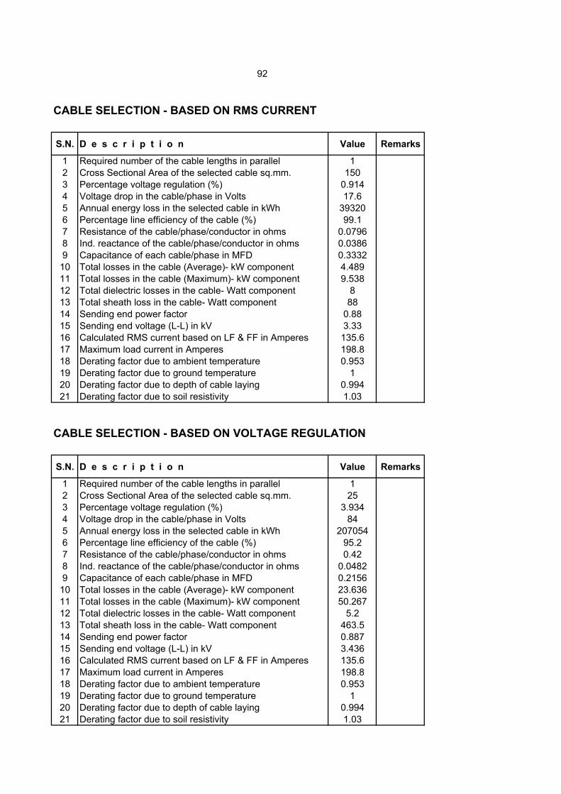
CABLE SELECTION - BASED ON RMS CURRENT

S.N. D e s c r i p t i o n Value Remarks

1 Required number of the cable lengths in parallel 12 Cross Sectional Area of the selected cable sq.mm. 1503 Percentage voltage regulation (%) 0.9144 Voltage drop in the cable/phase in Volts 17.65 Annual energy loss in the selected cable in kWh 393206 Percentage line efficiency of the cable (%) 99.17 Resistance of the cable/phase/conductor in ohms 0.07968 Ind. reactance of the cable/phase/conductor in ohms 0.03869 Capacitance of each cable/phase in MFD 0.3332

10 Total losses in the cable (Average)- kW component 4.48911 Total losses in the cable (Maximum)- kW component 9.53812 Total dielectric losses in the cable- Watt component 813 Total sheath loss in the cable- Watt component 8814 Sending end power factor 0.8815 Sending end voltage (L-L) in kV 3.3316 Calculated RMS current based on LF & FF in Amperes 135.617 Maximum load current in Amperes 198.818 Derating factor due to ambient temperature 0.95319 Derating factor due to ground temperature 120 Derating factor due to depth of cable laying 0.99421 Derating factor due to soil resistivity 1.03

CABLE SELECTION - BASED ON VOLTAGE REGULATION

S.N. D e s c r i p t i o n Value Remarks

1 Required number of the cable lengths in parallel 12 Cross Sectional Area of the selected cable sq.mm. 253 Percentage voltage regulation (%) 3.9344 Voltage drop in the cable/phase in Volts 845 Annual energy loss in the selected cable in kWh 2070546 Percentage line efficiency of the cable (%) 95.27 Resistance of the cable/phase/conductor in ohms 0.428 Ind. reactance of the cable/phase/conductor in ohms 0.04829 Capacitance of each cable/phase in MFD 0.2156

10 Total losses in the cable (Average)- kW component 23.63611 Total losses in the cable (Maximum)- kW component 50.26712 Total dielectric losses in the cable- Watt component 5.213 Total sheath loss in the cable- Watt component 463.514 Sending end power factor 0.88715 Sending end voltage (L-L) in kV 3.43616 Calculated RMS current based on LF & FF in Amperes 135.617 Maximum load current in Amperes 198.818 Derating factor due to ambient temperature 0.95319 Derating factor due to ground temperature 120 Derating factor due to depth of cable laying 0.99421 Derating factor due to soil resistivity 1.03

92

CABLES VOLTAGE REGULATION & DROP

S.N. Description Unit OUTPUT

1 Receiving end load shared by cable path kW 1502 Sending end voltage of the cable (L-L) kV 3.3023 Sending end current/ phase of the system Amps. 30.364 Sending end power factor of the system Factor 0.86445 Percentage voltage regulation of the system % 0.056 Annual energy losses in the cable(s) kWh 3357 Total losses (max. in eq. kW) in the system kW 0.088 Total line losses (rms eq. kW) in the system kW 0.049 Resist./phase/cond. of the cable at 75°C Ohms 0.0295

10 Inductive react./phase/cond. of the cable Ohms 0.007411 Line efficiency of the cable feeding system. % 99.9512 Receiving end current/ phase in cable(s) Amps. 30.5213 Form factor of the system. Factor 1.2214 Total Capacitance/ phase of the cable(s) MFD 0.515 Receiving end capacitor current Amps. 0.0516 Cable line mid point capacitor current Amps. 0.217 Sending end capacitor current Amps. 0.0518 Capacitive react./phase/cond. of the cable k.Ohms 6.419 Equivalent impedance/ phase of cable(s) Ohms 0.030520 Type of conductor material of the cable Type cu21 Cross sectional area of cable(s) sq.mm. 7022 Current carrying capacity of cable(s) Amps. 16523 Voltage DROP per phase in the cable(s) Volts 0.9

93

SN MeterNo BillCycle Bill Number Contract Demand

Units_ cons Tot_Bill

1 NKC-TVMSEMWBB02626 1/02/04 51040200156 2000 772560 25218922 LKC-TVMSEMWBB02627 1/02/04 51040200158 1600 479232 15704583 CLJ-TVMSEMWBU02081 1/02/04 51040200056 750 224436 7345584 BH-RJ-TVMSEMWBD01710 1/02/04 51040200053 1000 370584 12114005 BH-PJ-TVMSEMWBB00671 1/02/04 51040200057 850 268696 8790336 BH-NJ-TVMSEMWBU02088 1/02/04 51040200159 1100 349500 11462707 HRP-TVMSEMWBB02637 1/02/04 51040200048 1300 413860 13648508 BH-PJ-TVMSEMWBB00671 1/03/04 51040300038 850 272336 8908949 LKC-TVMSEMWBB02627 1/03/04 51040300148 1600 597960 1957733

10 BH-RJ-TVMSEMWBD01710 1/03/04 51040300034 1000 445008 145414911 NKC-TVMSEMWBB02626 1/03/04 51040300146 2000 899160 293483212 HRP-TVMSEMWBB02637 1/03/04 51040300009 1300 461920 152161513 CLJ-TVMSEMWBU02081 1/03/04 51040300037 750 271020 88650914 BH-RJ-TVMSEMWBD01710 1/01/04 51040100081 1000 403092 131743815 BH-PJ-TVMSEMWBB00671 1/01/04 51040100089 850 271144 88701916 BH-NJ-TVMSEMWBU02088 1/03/04 51040300149 1100 389870 127791517 HRP-TVMSEMWBB02637 1/01/04 51040100166 1300 475100 156460718 NKC-TVMSEMWBB02626 1/01/04 51040100037 2000 867360 283108519 CLJ-TVMSEMWBU02081 1/01/04 51040100087 750 222136 72705620 BH-NJ-TVMSEMWBU02088 1/01/04 51040100163 1100 401870 131709521 LKC-TVMSEMWBB02627 1/01/04 51040100189 1600 399816 1323303

G R A N D T O T A L 1229 9256660 30319711AVERAGE

OHL COST BREAK-UP

S.N. ITEM DESCRIPTION UNIT QNTY. UNIT RATE AMOUNT IN Rs.

1 ACSR 'DOG ' Conductor having eq. Al csa=105 mm²

km 3.3 42849 141404

2 Rail Pole (52kg/m) '9 metres' height

no. 12 16050 192600

3 11kV Disc Type Insulators no. 36 963 346684 Line Hardwares-

brackets/clamps etc.set 12 368 4424

5 7x2.59 mm Galvanized Earth Wire

km 1.1 17922 19715

6 PCC Work at Pole/ Tower Sites no. 12 553 6636

7 Earthings at Pole/ Tower Sites no. 2 986 1972

SUB-TOTAL 4014198 Transportation, erection,

bracket and insulator fitting, wire stranding, supervision etc.

LS 25% 401419 100354

GRAND-TOTAL 501774Rupees Fifty Lakh One Thosand Seven Hundred SeventyFour Only.

DISPLAY OF 3 SELECTED FIELDS DATA OF 8 METERS (21 FOUND)

TOTAL

94

95 POWER BALANCE FOR UNDERGROUND PROJECT

SUPERPOSITION METHOD

Sl. No. Description

Connected Load in

kW

Working Load in

kW Demand Factor

Power Factor (cos ø)

tan ø Apparent

load in kW

Reactive load in kVAr

Maximum Demand in

kVA

Running Hours/

day

Annual Working

days

Annual Consump. In MkWh

1 Vertical Transport 400 200 0.80 0.85 0.62 160 99 188 10 300 0.4802 Pumping 1200 1000 0.80 0.85 0.62 800 496 941 16 365 4.6723 Surface Lighting 300 100 0.90 0.90 0.48 90 44 100 12 365 0.3944 Underground lighting 200 200 0.90 0.90 0.48 180 87 200 24 365 1.5775 Colony 750 500 0.80 0.85 0.62 400 248 471 10 365 1.4606 Direct Haulage 800 600 0.80 0.80 0.75 480 360 600 15 300 2.1607 Endless Haulage 70 35 0.80 0.80 0.75 28 21 35 15 300 0.1268 Belt Conveyor 100 70 0.80 0.75 0.88 56 49 75 15 300 0.2529 CHP 200 150 0.80 0.80 0.75 120 90 150 12 300 0.43210 Compressor 200 100 0.60 0.70 1.02 60 61 86 10 300 0.180

Sub-Total 4220 2955 0.80 0.84 0.66 2374 1555 2838 11.733 Superposition factors 0.925 For kW 0.964 For kVAr 2955 0.74 0.83 0.68 2196 1499 2659 Improving PF upto 0.95 2955 0.74 0.95 0.33 2196 722 2311 Capacitor Bank required for power factor improvement in kVAr 260 x 3 kVAr Required Transformer Capacity in kVA 1387 x 2 kVA Selected Transformer Capacity in kVA 1600 x 2 kVA Percentage Voltage Impedance of the Selected Transformer 6.25 %

96 POWER BALANCE FOR UNDERGROUND PROJECT

DIVERSITY FACTOR METHOD

Sl. No. Description

Connected Load in

kW

Working Load in

kW Demand Factor

Power Factor (cos ø)

tan ø Apparent

load in kW

Reactive load in kVAr

Maximum Demand in

kVA

Running Hours/

day

Annual Working

days

Annual Consump. In MkWh

1 Vertical Transport 400 200 0.8 0.85 0.620 160 99 188 10 300 0.480 2 Pumping 1200 1000 0.8 0.85 0.620 800 496 941 16 365 4.672 3 Surface Lighting 300 100 0.9 0.9 0.484 90 44 100 12 365 0.3944 Underground lighting 200 200 0.9 0.9 0.484 180 87 200 24 365 1.5775 Colony 750 500 0.8 0.85 0.620 400 248 471 10 365 1.460 6 Direct Haulage 800 600 0.8 0.8 0.750 480 360 600 15 300 2.1607 Endless Haulage 70 35 0.8 0.8 0.750 28 21 35 15 300 0.1268 Belt Conveyor 100 70 0.8 0.75 0.882 56 49 75 15 300 0.252 9 CHP 200 150 0.8 0.8 0.750 120 90 150 12 300 0.432

10 Compressor 200 100 0.6 0.7 1.020 60 61 86 10 300 0.180 Sub-Total 4220 2955 0.80 0.84 0.655 2374 1555 2838 11.733 Taking Diversity factor for kW and kVAr as 1.23 2955 0.65 0.84 0.655 1930 1264 2307 Improving PF upto 0.95 2955 0.65 0.95 0.329 1930 634 2032 Capacitor Bank required for power factor improvement in kVAr 210 x 3 kVAr Required Transformer Capacity in kVA 1219 x 2 kVA Selected Transformer Capacity in kVA 1250 x 2 kVA Percentage Voltage Impedance of the Selected Transformer 5 %

97 RESULTS OF SAG TENSION CALCULATIONS

Temp. Description of OHL Cond.+Ice Wind load Eqv. load Stress Tension Tension SagDefl SagVert SagHrz Remarksin °C / c o n d i t i o n kg/m. kg/m. kg/m. kg/sq.cm. in kg % UTS in mm in mm in mm

5 WITH FULL WIND LOAD 0.726 2.743 2.838 1852 3593 53.5 10688 2735 10332 Ok, Tension within the limit of 70%. 5 WITH 36% WIND LOAD 0.726 0.988 1.226 1317 2555 38 3036 1798 2446 Swing from vertical = 75.2° at full wind 5 WITHOUT WIND LOAD 0.726 0 0.726 1148 2227 33.1 2063 2063 0 Swing from vertical = 53.7° at 36% wind ** Assumed Factor of Safety = 4.00 at 25% UTS

32 WITH FULL WIND LOAD 0.726 2.743 2.838 1663 3227 48 5564 1424 5379 32 WITH 36% WIND LOAD 0.726 0.988 1.226 1078 2092 31.1 3707 2196 298632 WITHOUT WIND LOAD 0.726 0 0.726 866 1680 25.0** 2735 2735 0 Ok, Tension within the limit of 25%.

75 WITH FULL WIND LOAD 0.726 2.743 2.838 1423 2762 41.1 6502 1663 6285 75 WITH 36% WIND LOAD 0.726 0.988 1.226 812 1575 23.4 4925 2917 396875 WITHOUT WIND LOAD 0.726 0 0.726 571 1109 16.5 4144 4144 0

32 No wind load (Initial) 0.726 0 0.726 527 1022 15.2 4496 4496 0 Ok, Tension within the limit of 35%. 32 Initial with wind load 0.726 2.743 2.838 1307 2535 37.7 7082 1812 6846

INPUT DATA VALUE VALUE INPUT DATA Conductor name WOLF 6260 Initial Modulus of Elasticity in kg/m² Conductor dia. in mm. 18.13 8158 Final Modulus of Elasticity in kg/m² Cond. CS Area in mm² 194.04 151.3 Wind pressure in kg/m² Conductor Wt. in kg/m 0.726 70 % Limiting tension (Worst at given °C) Conductor UTS in kg 6720 35 % Initial limiting tension OHL normal span in m 225 25 % Limiting tension (No wind at given °C) OHL ruling span in m 200 0 Thickness of ice in mm Minimum temp. in °C 5 0.9168 Specific gravity of ice Everyday temp. in °C 32 17.78 x 10^(-6) Coeff. of linear exp./°C Maximum temp. in °C 75 ...Generated by Elect 7.05 on 26/11/04 at 9:21:55 PM

98

ENERGY BILL ANALYSIS TREND OF BILL AMOUNT OF SINGLE METER - GRAPHICAL VIEW

COMPARATIVE VIEW OF UNITS CONSUMED DURING A PERIOD BY NUMBER OF METERS - GRAPHICAL VIEW

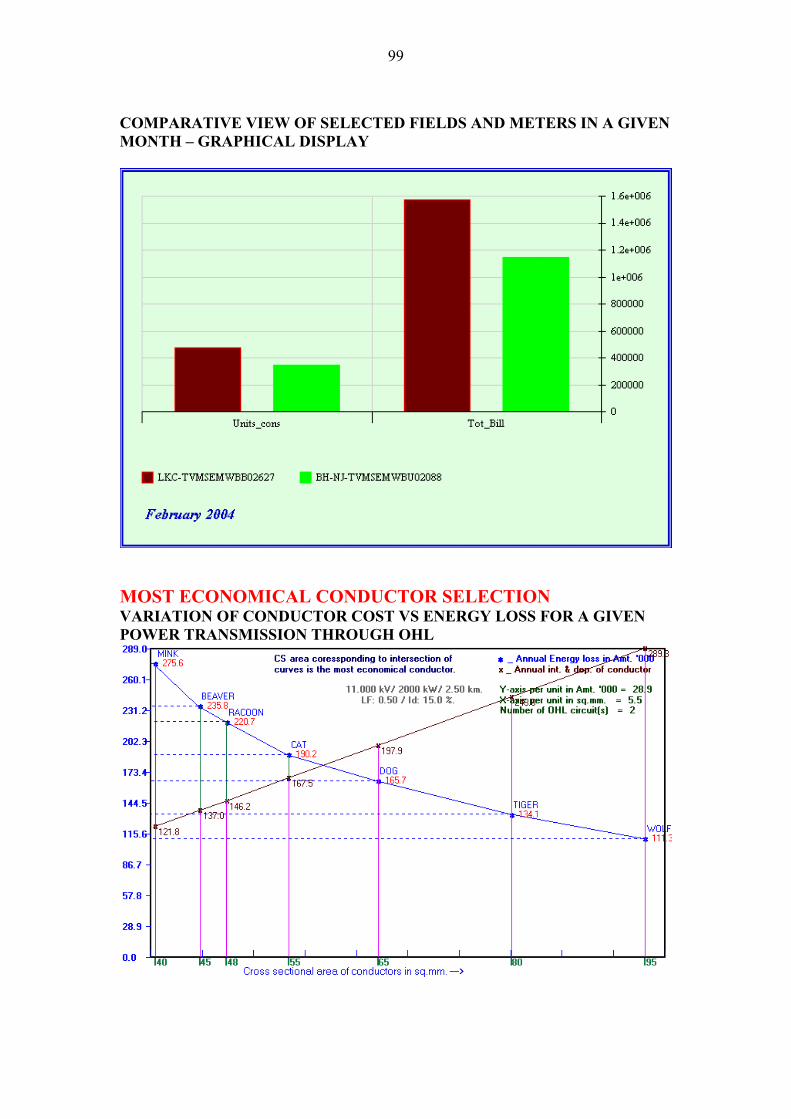
99

COMPARATIVE VIEW OF SELECTED FIELDS AND METERS IN A GIVEN MONTH – GRAPHICAL DISPLAY

MOST ECONOMICAL CONDUCTOR SELECTION VARIATION OF CONDUCTOR COST VS ENERGY LOSS FOR A GIVEN POWER TRANSMISSION THROUGH OHL

100

PROPERTIES OF OVERHEAD LINE CONDUCTORS Conductors are formed with a number of stranded aluminium wires. To strengthen the conductor, steel wires are used in the core of the strands. It is always better to use steel wires in the inner section because of the lower current density in the inner part, compared to outer part of the conductor section. The higher resistivity of steel thus has a very little effect on voltage drop and regulation. Two types of conductors are in common use:

1. ACSR (Aluminium Conductor Galvanised Steel Reinforced) 2. AAAC (All Alloy Aluminium Conductor)

One more type AAC (All Aluminium Conductor) is also in use, but is being replaced by AAAC due to superior quality of AAAC over AAC. In ACSR Conductors, normally the core is made up of steel wires to strengthen the tensile properties. Numbers of layers are then placed over this core to form the desired size of conductors. There are standards for the size of wire sections both of steel and aluminium. In normal practice, both steel and aluminium wires of conductors are kept of the same size or else the outer diameter of steel core is approximately equal to diameter of individual aluminium wires. This is done to reduce the spacing factor of the conductor i.e. to make the conductor more compact. The maximum number of wires that can be placed over a layer is given by 6n, where n is layer number. The constant 6 is the integer value of 2π. Thus; wire arrangement in the section of a 4-layer conductor will be as under:

CORE - 1 LAYER 1 - 6 LAYER 2 - 6x2 LAYER 3 - 6x3 LAYER 4 - 6x4 TOTAL - 61

In AAAC type overhead line conductors, the construction is same as above, except the core, which is also of aluminium instead of steel. The breaking load/ tensile strength (UTS) of AAAC is comparable to ACSR, rather it is better than ACSR. The resistance and current density qualities of AAAC are also superior to those of same size of ACSR. The only poor part of AAAC is that it can be cut more easily than ACSR. Consider the following variables for further discussion:

an = Number of Aluminium wires

sn = Number of Steel wires

101

ad = Outer diameter of Aluminium wires in mm

sd = Outer diameter of Steel wires in mm 1. OVERALL RADIUS OF CONDUCTOR For a conductor made up of a given number of Aluminium/ Steel wires of given outer diameters, the overall radius rd of the conductor so formed is given by:

( 2/2 asd ddr += ))))

For 1 steel and 6 aluminium stranded conductor (7 Strands) ( 2/23 asd ddr += For 7 steel and 6 aluminium stranded conductor (13 Strands) ( 2/43 asd ddr += For 7 steel and 30 aluminium stranded conductor (37 Strands) ( 2/63 asd ddr += For 7 steel and 54 aluminium stranded conductor (61 Strands)

These empirical relations are required to assess the inductance and capacitance of the overhead line comprised of these conductors. The above relations may be generalized for n layers conductor over the central core, the diameters of component wires being equal: ( ) 2/12 ad dnr ×+= 2. EQUIVALENT ALUMINIUM AREA (eqa) Equivalent aluminium area of the composite conductor formed of Aluminium and steel may be given by:

×+=

sistivitySteelsistivityAlAreaSteelTotalAreaAlTotaleqa

Re_Re_____

or

×+=

s

alAreaSteelalaeqaρρ

_

3. NOMINAL EQUIVALENT COPPER AREA (eqc) To find the nominal equivalent copper area, the first step is to convert the equivalent aluminium area to equivalent copper and then set this value to the nearest standard value as specified in standards:

iumAlusistivityCoppersistivityareaAleqeqc

min_Re_Re__ ×

=

or

×

al

cueqaρρ

=eqc

102

4. CURRENT CARRYING CAPACITY (CCC) & CURRENT DENSITY The current density in a section of conductor is not uniform. The practical values of current density show it to vary exponentially. The author has arrived at the following empirical relationships for current density in different types and cross sectional area of conductors:

0.2

0.3

0.4

0.5

0.6

0.7

0.8

0.9

1

1.1

1.2

0 100

Den

sity

A/m

m²

ACSR AAAC

CURRENT DENSIT

Empirical relation of the AC

2.08642.0)log( −=δ

or e 8642.0=δ

Empirical relation of the AA

34.0137.1)log( −=δ

or e 137.1 −=δ Based on the above empiriccapacity of different size of c

arequivAlCondccc ___=

or 8.0eeqaccc ×=

And 1.1eeqaccc ×=

ACSR

200 300

Al A

C

Y CURVES FO

SR curve (show

( )eqalog385×(eqalog2385.0 ×−

AC curve (sho

( )eqalog68×

( )eqalog3468.0 ×

al relations ofonductors may

dCurrentea _×log(2385.0642 e×−

log(3468..037 e×−

AAA

400 500 600 700 800

rea in mm²

R ACSR & AAAC CONDUCTORS

n black) is given by:

)

wn pink) is given by:

the current density, the current carrying be calculated out as under:

ensity

For ACSR )qa

For AAAC )qa

103

5. RESISTANCE (R at 20°C) ACSR CONDUCTORS Let Steel wires= ns numbers each of diameter ds mm. Aluminium wires= na numbers each of diameter da mm Resistvity of steel = stρ Resistvity of aluminium = alρ

Equivalent aluminium area st

alareasteelareaalρρ

×+= __ eqa

or st

aldsnsdanaeqaρρππ

×××+××= 22

44

Resistance/km in Ohms eqa

R alρ= Where alρ is in Ω kmmm /2

NOTE: IS 398 (Part-III)-1976 neglects the conductivity of steel core and calculates resistance

taking a factor for accounting stranding and lay ratio. AAAC/AAC CONDUCTORS

Equivalent aluminium area 2

4dana ××=

πala

Resistance/km in Ohms eqa

R alρ= Where alρ is in Ω kmmm /2

NOTE: IS 398 (Part-III)-1976 calculates resistance taking a factor for accounting stranding

and lay ratio. Resistance at any other temperature than 20°C is given by:

++

=205.241

5.24120

tRRt

6. REACTANCE (xl and xc) Inductance L in Henry/m of the overhead line comprised of conductors of radius r mm and spacing between conductors d mm is given by the following formula:

710ln25.0 −×

×+

rd

=L Henry/m

Corresponding inductive reactance per km of the overhead line is thus given by:

×+

rd

l ln25.0100π

=x Ohms/km

104

And Capacitance C in microfarad/km of the overhead line comprised of conductors of radius r mm and spacing between conductors d mm is given by the following formula:

×

rdln18

1=C mfd/km

Corresponding Capacitive reactance per km of the overhead line is thus given by:

f

rd

fCc ππ 2

ln1018

21

6

××

=x = Ohms/km

Note: From the above equations of xl and xc it may be noted that both the inductive

and capacitive reactance depend on the spacing between conductors of the overhead line. Further, the spacing between overhead line conductors depends on the system voltage, span, sag, weather conditions etc. The values calculated are for a default conductor spacing of 700 mm.

7. WEIGHT OF CONDUCTOR ACSR CONDUCTORS Weight/Mass of ACSR conductor/km = (Vol. of steel/km) x Steel_density + (Vol. of Al/km) x Al_density

als dadsW δπ

δπ

××+××= 22

44

Where ds and da in mm and δ in gm/cc (or kg/litre) sδ al

AAAC/AAC CONDUCTORS Weight of AAAC conductor/km = (Vol. of Al/km) x Al_density

alda δπ

×× 2

4W =

Where da in mm δ in gm/cc (or kg/litre) al

NOTE: IS-398 (Part-II) & (Part-III) – 1976 takes mass of the conductor as the sum of

masses of individual wires multiplied by a factor which accounts for stranding of wires (because the length of stranded wires are greater than that of central wire).

105

8. TENSILE STRENGTH Tensile strength/ breaking load of conductor is taken as 98 percent of the sum of the breaking loads of the aluminium wires plus 85 percent of the sum of breaking loads of the component wires before stranding. VOLTAGE REGULATION LIMITS IN OH LINES RULE 54 & 55 OF INDIAN ELECTRICTY RULE- 1956 (AMMENDED UPTO 1st JULY 1990) 54. Declared voltage of supply to consumer – Except with the written consent or with

the previous sanction of the State Government a supplier shall not permit the voltage at the point of commencement of supply as defined under Rule 58 to vary from the declared voltage:

(i) in the case of low or medium voltage, by more than 6 per cent, or; (ii) in the case of high voltage, by more than 6 per cent on the higher side

or by more than 9 per cent on the lower side, or; (iii) in the case of extra high voltage, by more than 10 per cent on the

higher side or by more than 12.5 per cent on the lower side. 55. Declared frequency of supply to consumer – Except with the written consent or

with the previous sanction of the State Government a supplier shall not permit the frequency of an alternating current supply to vary the declared frequency by more than 3 per cent.