1

Behavioural Equilibrium Exchange Rate and Total Misalignment: Evidence from the Euro Exchange Rate

Nikolaos Giannellis

Department of Economics, University of Peloponnese, Greece Telephone: +302251041898

Fax: +302251028160

e-mail: gianelis@uop.gr

Minoas Koukouritakis (corresponding author)

Department of Economics, University of Crete, Greece Telephone: +302831077411

Fax: +302831077406

e-mail: minoas@econ.soc.uoc.gr

Abstract: This paper investigates whether the nominal euro exchange rate against the currencies

of China, Japan, the UK and the USA converges or not to its equilibrium level. Applying

cointegration and common trend techniques in the presence of structural breaks in the data, we

found a valid long-run relationship between the euro/yuan, euro/yen, euro/UK pound and euro/US

dollar nominal exchange rates and the fundamentals defined by the monetary model. Our modified

Behavioural Equilibrium Exchange Rate model suggests that at the end of the estimated period, the

euro/Chinese yuan and the euro/UK pound exchange rates follow an equilibrium process. On the

other hand, the euro is considered as overvalued against the US dollar and as undervalued against

the Japanese yen.

Keywords: Euro, BEER, Misalignment Rate, Cointegration, Structural Shifts

JEL Classification: E43, F15, F42

2

1. Introduction

The present paper aims to evaluate the dynamic behaviour of the single European

currency. We attempt to examine the likelihood of emergence of significant future

fluctuations of the euro exchange rate against four major currencies, namely the

Chinese yuan, the Japanese yen, the UK pound and the US dollar. Future

exchange rate instability is not expected to be high if the above nominal exchange

rates are not significantly away from their equilibrium rates. The intuition is that

even if the exchange rate is currently stable but, significantly misaligned, the

exchange rate is going to be highly unstable in the future. Exchange rate volatility

corresponds to short-run fluctuations of the exchange rate around its long-run

trends, while exchange rate misalignment refers to a significant deviation of the

observed exchange rate from its equilibrium rate. Both notions are closely related

each other. This is because a highly misaligned exchange rate is going to be

highly volatile at present and in the future in order to find its equilibrium rate (by

its own forces or by government interventions in the foreign exchange market).

Given that the exchange rate is the link of the domestic economy with the rest

of the world, a significant misaligned exchange rate can have important negative

consequences on the Euro area. For instance, when euro is undervalued (below its

equilibrium rate) the economy is expected to face inflationary pressures. On the

other hand, if euro is overvalued (above its equilibrium rate) a competitiveness

problem is more possible for the Euro area. These situations suggest the necessity

of estimating the equilibrium exchange rate of the euro against the currencies of

Euro area’s major trading partners.

Departing from traditional theories of equilibrium exchange rates, such as the

Purchasing Power Parity, Williamson (1985) proposed the “Fundamental

Equilibrium Exchange Rate” (FEER), which is an alternative exchange rate

determination model suitable for medium-run analysis. The FEER approach

indicates that the exchange rate is at its equilibrium value when satisfies the

condition of simultaneous internal and external balance. Williamson interprets the

external balance condition in terms of current account balance and states that the

current account must be sustainable. Combining these two macroeconomic

conditions, the FEER is the rate that equates the current account at full

employment with sustainable net capital flows. Very close to FEER is the Desired

Equilibrium Exchange Rate (DEER) approach presented by Bayoumi et al (1994).

3

An additional approach about exchange rate determination is the Natural Real

Exchange Rate (NATREX), which is referred in both medium-run and long-run

periods. The NATREX is “…the rate that would prevail if speculative and

cyclical factors could be removed while unemployment is at its natural rate”

(Stein 1994, p. 135). This rate is consistent with simultaneous internal and

external balance and equates the sustainable current account with saving and

investment.

The latest approach for exchange rate determination is the Behavioural

Equilibrium Exchange Rate (BEER) proposed by Clark & MacDonald (1998).

The BEER is a short-run concept which involves the direct econometric analysis

of the exchange rate behaviour. It does not actually rely on any theoretical model

and the equilibrium rate is designated by the long-run behaviour of the

macroeconomic variables. Similarly, Clark & MacDonald (1998) proposed the

Permanent Equilibrium Exchange Rate (PEER) approach. The PEER approach

differs from BEER in the way that the exchange rate is a function only of those

variables that have a persistent effect on it.

This paper contributes to the literature of equilibrium exchange rate

determination by strengthening the theoretical background of the BEER model.

Our novelty lies on the fact that we combine the theoretical assumptions of the

monetary model of exchange rate determination (Frenkel 1976; Kouri 1976;

Mussa 1976, 1979) with the BEER methodology. This is an important issue, since

the BEER approach, whose building idea is the uncovered interest rate parity

(UIP) condition, does not actually rely on any theoretical model.

Furthermore, we account for structural breaks in the data. In our context, this is

also an important issue because the monetary and fiscal policies of the Euro area,

China, Japan, the UK and the USA are likely to have caused structural shifts in

the level and trend of the euro exchange rate vis-à-vis the Chinese yuan, the

Japanese yen, the UK pound and the US dollar. Since the presence of structural

breaks in the data are known to have significant effects on the properties and

interpretation of standard unit root and cointegration tests, we employ recently

developed tests that are valid in the presence of structural shifts in the data; we

discuss these issues extensively in section 3 below.

In what follows, first, we use monthly data available from the 1999:01 and unit

root tests in the presence of structural breaks in the data (Lee and Strazicich 2003,

4

2004), in order to test for stationarity and to determine endogenously the possible

structural breaks that exist.

Second, we use recently developed cointegration tests that allow for structural

breaks in the data (Johansen, Mosconi and Nielsen 2000, and Lütkepohl and his

associates in several papers noted below) in order to establish a valid long-run

relationship between the nominal euro exchange rate vis-à-vis the Chinese yuan,

the Japanese yen, the UK pound and the US dollar and the fundamental variables

that defined by the monetary model of exchange rate determination.

Third, from the above long-run relationship we estimate the total equilibrium

exchange rate (i.e. the BEER) in order to investigate if the nominal euro exchange

rate against the currencies of China, Japan, the UK and the USA is overvalued or

undervalued in relation to its equilibrium level.

In brief, our empirical results indicate that, at the end of our sample, the euro is

overvalued in relation to the US dollar, undervalued in relation to the Japanese

yen and moves towards its equilibrium value in relation to the Chinese yuan and

the UK pound.

The rest of the paper is organized as follows. Section 2 discusses the theoretical

framework of the BEER model and the way that this methodology can be

combined with the theoretical assumptions of the monetary model. Section 3

describes the data and outlines the unit root and cointegration tests in the presence

of structural breaks. Section 4 discusses the results for the current and total

equilibrium exchange rates, while section 5 contains some concluding remarks.

2. Theoretical Framework

2.1 The Model

The estimation of the equilibrium exchange rate is based on the BEER approach

of Clark and MacDonald (1998). This approach estimates the exchange rate

misalignment in accordance with the deviations of the actual exchange rate from

its estimated value, which is derived from the long-run relationship between the

exchange rate and the macroeconomic fundamentals. The advantage of the BEER

model is that the exchange rate is a function of variables that have a direct effect

on the exchange rate. In other words, the equilibrium exchange rate is driven by

5

the sustainable (equilibrium) values of the fundamentals that affect the actual

exchange rate in the long run and not by overall macroeconomic balance.

The BEER approach does not actually rely on any theoretical model and the

equilibrium rate is designated by the long-run behaviour of the macroeconomic

variables. However, this does not mean that any theoretical concept is not

required. Stein (2001) presents an evaluation of studies based on the BEER

approach, in which the authors have in mind a theoretical model but there is no

need to be specified. For example, most authors have in mind the condition of

simultaneous internal and external balance. This implies that the building idea of

the BEER approach is the UIP condition.

In this study, we strengthen the theoretical background of the BEER model by

assuming that the fundamentals that affect the long-run exchange rate are those

defined by the monetary model of exchange rate determination. Our approach

extends the standard BEER approach in the sense that we do rely on a theoretical

model.

The monetary model is briefly described as follows. Assuming that (a) prices

are flexible, (b) the economy is at full employment level and (c) the purchasing

power parity (PPP) and UIP conditions hold all the time, the domestic and foreign

monetary equilibrium conditions are described by equations (1) and (2),

respectively:

,t t t tm p y rϕ μ− = − (1)

* * * * * * ,t t t tm p y rϕ μ− = − (2)

* ,t t ts p p= − (3)

*1[ ] .t t t tr r E s += + Δ (4)

Equation (3) stands for the PPP condition, while equation (4) represents the UIP

condition. s is the nominal exchange rate (domestic currency per unit of foreign

currency) and , , ,m p y r represent the domestic real money supply, the domestic

price level, the domestic real income and the domestic interest rate, respectively. *

denotes the respective foreign variables.

The foreign price level is exogenous to the domestic economy and the domestic

money supply determines the domestic price level and hence the exchange rate.

Combining equations (1) and (2) and assuming that the domestic and foreign

coefficients are identical, the relative money demands are given by

6

* * * *( ) ( ) ( ) ( )t t t t t t t tm m p p y y r rϕ μ− − − = − − − (5)

Solving for the relative prices and using the PPP condition, we get the exchange

rate equation, which is the main expression of the monetary model:

* * *( ) ( ) ( )t t t t t t ts m m y y r rφ μ= − − − + − (6)

Equation (6) shows that the nominal exchange rate depends on the relative money

supply, the relative output, and the interest rate differential. Applying the UIP

condition, equation (6) becomes:

* *1( ) ( ) [ ]t t t t t t ts m m y y E sφ μ += − − − + Δ (7)

Since the PPP holds all the time, it turns out that *1 1 1[ ] [ ] [ ]t t t t t tE s E Eπ π+ + +Δ = − ,

where π and *π are the domestic and foreign inflation rates, respectively. Then

the exchange rate equation becomes:

* * *1 1( ) ( ) ( [ ] [ ])t t t t t t t t ts m m y y E Eφ μ π π+ += − − − + − (8)

Finally, assuming that inflation expectations are rationally formed (i.e. the market

agents have perfect foresight), we derive the long-run exchange rate (or,

equivalently, the current equilibrium exchange rate):

* * *1 1( ) ( ) ( )t t t t t t ts m m y yφ μ π π+ += − − − + − (9)

According to the monetary model, the sign of the money supply differential is

expected to be positive, which means that if the increase of the domestic money

supply is greater than this of the foreign money supply, the domestic currency is

expected to depreciate. This happens because the increased money stock increases

the domestic price level and thus, the domestic goods become less competitive

than the foreign ones. Thus, demand for domestic goods decreases and this of

foreign goods increases.

The sign of the output differential is expected to be negative, which means that

a relative higher increase in the domestic output will appreciate the domestic

currency. This happens because the increase of the domestic product will increase

the demand for money and given the money supply unchanged, there will be

excess demand for the domestic money stock. The money market equilibrium will

be restored if people reduce their expenditure on consumption. Domestic prices

fall and through the PPP, the exchange rate decreases.

Also, the sign of the inflation rate differential is expected to be positive.

Starting from equation (6) and following the steps to derive equation (9) we

observe that the effect of the inflation rate differential on the exchange rate is

7

correlated with the effect of the interest rate differential. The response of the

exchange rate to an increase in the domestic interest rate has exactly the opposite

effect with an increase in the domestic output. A higher interest rate will decrease

the demand for money and given the money supply unchanged, the domestic price

level increases. As a consequence, foreign goods are preferable to domestic goods

since they are cheaper. The trade balance deteriorates and the domestic currency

depreciates. Besides this effect, an increase in the domestic interest rate implies

expectations of higher future domestic inflation rate. This will create expectations

of depreciation of the domestic currency and agents with perfect foresight will sell

domestic currency for foreign currency. It is obvious that, through this

mechanism, a relatively higher expected inflation in the future is going to

depreciate the domestic currency at the present. Thus, given the assumption of

rational expectations, the future inflation rate differential is expected to enter the

exchange rate equation with a positive sign.

2.2 Equilibrium Exchange Rate and Total Misalignment

Following Clark and MacDonald (1998) we set as 1Z a vector of macroeconomic

fundamentals that affect the exchange rate in the long run, as 2Z a vector of

macroeconomic fundamentals that affect the exchange rate in the medium run and

as T a vector of variables that affect the exchange rate in the short run. Then, the

nominal exchange rate is defined as follows:

1 1 2 2t t t t ts Z Z T uβ β τ= + + + (10)

where, 1 2,β β and τ are reduced form coefficients and tu is the error term.

The current values of the medium-run and long-run fundamentals give the current

equilibrium exchange rate, which is expressed by equation (11) below. By

subtracting (11) from (10), we get the current misalignment, which is expressed

by equation (12).

1 1 2 2t t ts Z Zβ β= + (11)

t t t ts s T uτ− = + (12)

Equation (11) is equivalent to equation (9) if 1Z and 2Z are filled with the

variables of the monetary model. Equation 12 corresponds to the series that results

by subtracting equation (9) from the actual exchange rate.

8

What actually matters in our analysis, is the total misalignment that is the

deviation of the actual exchange rate from the total equilibrium exchange rate. To

estimate the total misalignment, we replace 1Z and 2Z in equation (10) with the

long run (or equilibrium) values of the fundamentals, 1Z and 2Z , respectively. In

other words, the total equilibrium exchange rate (BEER) is estimated by filtering

the fundamentals from speculative and cyclical factors. Maintaining the

theoretical affairs of the monetary model, the BEER is given by:

* * *1 1( ) ( ) ( )t t t t t tBEER m m y yϕ μ π π+ += − − − + − (13)

Comparing the BEER with the actual exchange rate we find how the latter

deviates from the former. If the actual exchange rate, ts , exceeds the BEER, the

exchange rate is said to be overvalued, while if the actual exchange rate is less

than the BEER, the exchange rate is undervalued. Thus, the total misalignment

rate is given by

1 1 2 2t t t ts Z Zξ β β= − − (14)

Finally, by adding and subtracting the current equilibrium exchange rate, s ,

from the right-hand side of equation (14) and using equation (12), we can

decompose the source of exchange rate misalignment,ξ :

1 1 1 2 2 2( ) ( ) ( )t t t t t t tT u Z Z Z Zξ τ β β= + + − + − (15)

Equation (15) illustrates the sources of exchange rate deviation from its

equilibrium value. These are: (i) the transitory factors that have a short-run effect

on the exchange rate, (ii) the disturbance term and, finally and more importantly,

(iii) the deviations of the macroeconomic fundamentals from their long-run (or

equilibrium) values.

Since one of the novelties of the present paper is that we take into account the

presence of structural breaks in the data, we describe in section 3 below the two-

and one-break LM unit root tests and system cointegration tests in the presence of

structural breaks. These tests will be used in the subsequent analysis in order to

estimate the BEER for the euro/Chinese yuan, euro/Japanese yen, euro/UK pound

and euro/US dollar exchange rates.

9

3. Unit Roots and Cointegration with Structural Breaks

Table 1 presents the data that we used in the present paper along with their

sources. Our sample is consisted of monthly observations from 1999:01 to

2008:08. During this period several events have taken place in the economies of

China, the EMU, Japan, the UK and the USA, which are likely to have caused

structural breaks in their time series. Since the presence of structural breaks is

known to have significant effects on the properties and interpretation of standard

ADF-type unit root tests and Johansen-type cointegration tests, we employ, as

noted above, recently developed tests that are valid in the presence for structural

shifts.

3.1 Unit Root Tests with Structural Breaks

We test for unit roots in the data using the two-break and one-break LM

(Lagrange Multiplier) tests that developed by Lee and Strazicich (2003, 2004).

These tests have several desirable properties: (a) they determine the structural

breaks “endogenously” from the data, (b) their null distributions are invariant to

level shifts in a variable, and (c) they are easy to interpret; by including breaks

under both the null and alternative hypotheses, a rejection of the null hypothesis

of a unit root implies unambiguously trend stationarity.

Consider the two-break LM unit root test for the process ty generated by

( )2, 1' ( ) , ~ 0,t t t t t t ty Z e e e A L iid Nδ β ε ε σ−= + = +

(16)

where A(L) is a k-order polynomial in the lag operator L and tZ is a vector of

exogenous variables whose components are determined by the type of breaks in

the process ty . Lee and Strazicich (2003) extend Perron’s (1989, 1993) single-

break models to include two breaks in the level (Model A) and two breaks in both

the level and trend (Model C) of ty . For Model A, 1 2[1, , , ]'t t tZ t D D= where

1jtD = for 1, 1,2Bjt T j≥ + = , and zero otherwise. For Model C,

1 2 1 2[1, , , , , ] 't t t t tZ t D D DT DT= , where jt BjDT t T= − for 1, 1,2Bjt T j≥ + = , and

zero otherwise. BjT denotes the point in time the break occurs.

10

It is clear from equation (16) that ty has a unit root if 1β = . Alternatively it is

trend stationary if 1β < . According to the LM principle, a unit root test statistic

can be obtained from the test regression

1 1' k

t t t i t i tiy Z S S uδ φ θ− −=

Δ = Δ + + Δ +∑ , (17)

where , 2,...,t t x tS y Z t Tψ δ= − − = , in which δ is a vector of coefficients in the

regression of tyΔ on tZΔ and 1 1x y Zψ δ= − , where 1y and 1Z are the first

observations of ty and tZ , respectively, and tu is an error term that is assumed to

be independent and identically distributed with zero mean and finite variance. The

lagged differences of t iS − are included as necessary to correct for serial

correlation in tu . The unit root null hypothesis is described by 0φ = in equation

(17) and can be tested by the LM test statistic:

tτ = -statistic for the hypothesis 0φ = . (18)

In order to endogenously determine the location of the two breaks

( , 1, 2j BjT T jλ = = , where T is the sample size) the two-break minimum LM test

statistic is determined by a grid search overλ :

( ){ }infLMτ λ τ λ= (19)

The critical values for this test are invariant to the break locations ( )jλ for Model

A but depend on the break locations for Model C. They are also available in Lee

and Strazicich (2003).

In this study, when the two-break LM test results showed that only one

structural break is significant for some variables, we computed the one-break LM

test of Lee and Strazicich (2004). We did this not only because the one-break LM

test appears more appropriate, but also because we wanted to determine if

including two breaks instead of one can adversely affect the power to reject the

unit root hypothesis for these variables.

3.2 Cointegration Tests with Structural Breaks

As in the case with unit root testing, structural breaks in the data can distort

substantially standard inference procedures for cointegration. Thus, it is necessary

to account for possible breaks in the data before inference on cointegration can be

made. In the recent cointegration literature in a VAR framework, there are two

11

main approaches. One developed by Johansen, Mosconi and Nielsen (2000)

(JMN) extends the standard VECM with a number of additional dummy variables

in order to account for q possible exogenous breaks in the levels and trends of the

deterministic components of a vector-valued stochastic process. JMN derive the

asymptotic distribution of the likelihood ratio (LR) or trace statistic for

cointegration and obtain critical or p-values, for the multivariate counterparts of

models A and C with q possible breaks, using the response surface method.

Consider the simple case with only level shifts in the constant termμ of an

observed p − dimensional time series , 1,...,tY t T= , of possibly ( )1I variables.

JMN divide the sample observations into q sub-samples, according to the

location of the break points, each of length 1j jT T −− for 1,...,j q=

and 0 10 ... qT T T T= < < < = , such that the last observation in the j th sub-sample

is jT , while the first observation in the ( )1j + th sub-sample is 1jT + . They assume

the following VECM(k) for tY , conditional on the first k observations of each

sub-sample1 11,...,j jT T kY Y− −+ + :

11 ,1 1 2

, (0, )k k qt t t i t i ji j t i t ti i j

Y Y D Y g D iidNμ ε ε−

− − −= = =Δ = Π + + Γ Δ + + Ω∑ ∑ ∑ ∼ , (20)

where 1,.........,( )qμ μ μ= and 1, ,........., ,( ) 't t q tD D D= are of dimension ( )p q× and

( 1)q× , respectively, and the ,j tD ’s are dummy variables, such that , 1j tD = for

1 1j jT k t T− + + ≤ ≤ and , 0j tD = otherwise, for 1,....,j q= .

As is well known, the hypothesis of at most 0r cointegrating relations

( )00 r p≤ < among the components of tY can be stated in terms of the reduced

rank of the ( )p p× matrix Π , in which case it can be written as 'αβΠ = ,

whereα andβ are matrices of dimension ( )p r× . The cointegration hypothesis

can then be tested by the likelihood ratio statistic

( )0 1

ˆln 1pJMN ii r

LR T λ= +

= − −∑ (21)

where the eigenvalues ˆ 'j sλ can be obtained by solving the related generalized

eigenvalue problem, based on estimation of the VECM(k) in equation (20), under

the additional restrictions that ', 1,.....,j j j qμ αρ= = , where jρ is of dimension

12

1 r× . These restrictions are required in order to eliminate a linear trend in the level

of the process tY (Johansen et al. 2000).

The second approach developed by Lütkepohl and his associates (see among

others, Lütkepohl and Saikkonen 2000; Saikkonen and Lütkepohl 2000; Trenkler,

Saikkonen and Lütkepohl 2008) (LST). LST assume that the structural breaks

have occurred only in the deterministic part and do not affect the stochastic part of

the process tY . Thus, LST set up the data generation process (DGP) for tY by

adding its deterministic part tμ to its stochastic part tX , where the latter is an

unobservable zero-mean purely stochastic VAR process, and use appropriate

dummy variables to account for exogenous shifts in tμ . Given this setup, LST

propose a two-step procedure to test for cointegration. Firstly, they remove the

deterministic part using a generalized least squares procedure under the

hypothesis of 0r cointegrating relations (GLS de-trending). Secondly, they test for

cointegration in the de-trended series using their proposed LM-type and LR-type

test statistics. Several tests statistics can be derived depending on whether there

are level shifts only or shifts in both the level and the trend. Lütkepohl, Saikkonen

and Trenkler (2003) study the statistical properties of their tests in the case of

level shifts, and compare them to the JMN test. They find that the LR-type tests

perform better than the LM-type tests in finite samples. Further, their tests have

better size and power properties than the JMN test in finite samples.

For LR-type tests, consider the case of a single shift in the level of tY .

Assuming an exogenous break at time BT in the level of tμ , LST specify the

following DGP for tY

0 1 , 1,....,t t t t tY X t d X t Tμ μ μ δ= + = + + + = , (22a)

where t is a linear time trend, iμ ( )0,1i = and δ are unknown ( )1p× parameter

vectors, td is a dummy variable defined as 0td = for Bt T< and 1td = for Bt T≥ ,

and where the unobserved stochastic error tX is assumed to follow a VAR(k)

process with VECM representation

11 1

, (0, ), 1,...,kt t i t i t ti

X X X iidN t Tε ε−

− −=Δ = Π + Γ Δ + Ω =∑ ∼ . (22b)

It is also assumed that the components of tX are at most ( )1I variables and

cointegrated ( ). . 'i e aβΠ = with cointegrating rank 0r , where 00 r p< ≤ .

13

Given the DGP in equations (22a) and (22b), the first step of the LST approach

involves obtaining estimates of the parameter vectors 0μ , 1μ andδ using a

feasible GLS procedure under the null hypothesis ( ) ( )0 0 0:H r rank rΠ = vs.

( ) ( )1 0 0:H r rank rΠ > (see Saikkonen and Lütkepohl 2000 for details). Having the

estimated parameters 0μ̂ , 1μ̂ and δ̂ , one can then compute the de-trended

series 0 1ˆˆ ˆ ˆt t tX Y t dμ μ δ= − − − . In the second step an LR-type test for the null

hypothesis of cointegration is applied to the de-trended series. This involves

replacing tX by ˆtX in the VECM (22b) and computing the LR or trace statistic:

( )0 1

ln 1pLST ii r

LR T λ= +

= − −∑ , (23)

where the eigenvalues 'i sλ can be obtained by solving a generalized eigenvalue

problem, along the lines of Johansen (1988).

Under the null hypothesis of cointegration, critical or p-values for a single level

shift can be computed by the response surface techniques (Trenkler 2008).

Trenkler et al. (2008) derive asymptotic results and p-values for the case of one

level shift and one trend break in the tY process, and show that, in this case, the

asymptotic distribution of the LR statistic in equation (23) depends on the location

of the break point. They also discuss how the results can be extended to the

general case of 1q > break points.

Since the JMN and LST approaches have different finite sample properties, we

employ both the JMNLR and LSTLR test statistics in our empirical analysis. The

break points are determined from the data on the basis of the results of the LM

unit root tests discussed above.

4. Empirical Results

4.1 Unit Root Results with Structural Breaks

Tables 2 and 3 report the unit root results from the two- and one-break LM tests,

respectively. We tested each time series for a unit root using the two-break LM

test at the 1-, 5- and 10 percent levels of significance. As noted above, when this

test showed that only one structural break is significant we employed the one-

14

break LM test at the same levels of significance. In order to determine the number

of lags, k , in equation (17), we used a “general to specific” procedure at each

combination of break points ( )1 2,λ λ for the two-break test, and at each single

break point λ for the one-break test. Initially, we set the lag-length at 12k = , and

examined the significance of the last lagged term, at the 10 percent level. The

procedure was repeated until the last lagged term was found to be significantly

different than zero, at which point the procedure stops.1

As shown in the last column of table 2, the unit root hypothesis with two

structural breaks cannot be rejected at any of the three levels of significance for all

nominal exchange rates, for the Euro area/USA output differential and for the

Euro area/China and Euro area/UK money supply differentials. It is also shown in

this column that the unit root hypothesis with two breaks is strongly rejected for

the Euro area/UK output differential and for the inflation rate differential in the

cases of Euro area/China, Euro area/UK and Euro area/USA. Table 3 reports the

results for the cases that one break is significant. As shown in the last column of

this table, the unit root hypothesis with one break cannot be rejected for the Euro

area/China and Euro area/Japan output differentials, for the Euro area/Japan and

Euro area/USA money supply differentials and for the Euro area/Japan inflation

rate differential.2 Since the results in table 3 are consistent with the results of table

2 regarding the null hypothesis, there does not seem to be any detectable loss of

power in using the two-break LM test to test the unit root hypothesis for the cases

of table 3. Finally, as shown in column 3 of tables 2 and 3, Model A with only

shifts in the deterministic levels fits the data best for Euro area/China and Euro

area/Japan cases, while Model C with shifts both in the levels and trends fits the

data best for the Euro area/UK and Euro area/USA cases, over the sample period.3

Column 5 of tables 2 and 3 reports the structural breaks in each series,

estimated from the data using the two-break and one-break LM tests, respectively.

Not surprisingly, the estimated breaks correspond closely to specific events that

have taken place, during the sample period, in the countries that we examine.

1 We computed the two-break and one-break LM tests using the Gauss codes of J. Lee available at the website http://www.cba.ua.edu/~jlee/gauss . 2 We also tested the interest rates of all countries for a second unit root. The null hypothesis was rejected in all cases. These results are available from the authors upon request. 3 Model A was chosen in the cases where the trend shift parameters in Model C were statistical insignificant at the 0.10 level.

15

Firstly, we examine the Euro area/China case. Our results indicate that the

money supply and inflation differentials appear a break in level in 2001. This

break coincides with a period where the European Central Bank (ECB) proceeded

to several reductions of its marginal lending facility rate (MLFR). At the same

time, China boosted bank lending and loosened its fiscal policy. These two actions

lead to an increase of the credit and money supply growth. In the end of 2002 and

in order to avoid “overheat” of the economy, the central bank of China tightened

its monetary policy in order to reduce aggregate demand. This action is may

reflected in the break in level of the output differential, in the beginning of 2003.

In 2004 and with the ECB’s MLFR unchanged at 3%, China tightened again its

monetary policy in order to fight inflation. This policy action coincides with the

structural break in the nominal exchange rate and inflation rate differential in that

year. The nominal exchange rate appears a second break in level in 2006, while

the money supply differential has a second break in early 2007. These breaks

coincide with a period of several increases of the ECB’s MLFR. Between March

2006 and March 2007, this rate increased from 3.5% to 4.75%.

Secondly, we examine the Euro area/Japan case. Our results indicate that the

nominal exchange rate appears to have two structural breaks in level, while each

of the output, money supply and inflation differentials has a single level shift. All

breaks have occurred between late 2000 and early 2001 and coincide with the

decisions of the Bank of Japan to (a) terminate the zero interest rate policy in

August 2000, which was implemented in February 1999, and (b) introduce

“quantitative easing” in March 2001, along with a zero interest rate again and with

a large expansion of monetary base. Unfortunately, these policy actions did not

help Japan to fight deflation successfully and to escape the “liquidity trap”.

Then, we examine the Euro area/UK case. As shown in tables 2 and 3, all

variables have two significant breaks in both the level and the trend. Our results

indicate that the output and inflation differentials appear to have a structural break

in mid-2000. The break in output differential coincides with the beginning of a

period that the UK economy started gradually to slow, while the break in the

inflation differential is probably related with the significant fall of the UK

inflation in that period. The inflation differential has a second break in mid-2001

which is probably related with an increase in the UK inflation. During the 2000-

2001 period, no remarkable changes were observed in the output growth and the

16

inflation rate of the Euro area. The nominal exchange rate and the money supply

differential appear to have a structural break at the end of 2002, which coincide

with the beginning of a period of several decreases of the ECB’s MLFR. Between

November 2002 and June 2003, this rate fell from 4.25% to 3%. During that

period, the UK rates remained unchanged. The output differential has a second

break at the end of 2003, which coincides with the beginning of a period of

increasing growth of the Euro area’s industrial production. Also, the nominal

exchange rate and the money supply differential have a second structural break in

2006. In that year, the ECB gradually raised its MLFR from 3.25% in January to

4.5% in December. In the same year, the Bank of England slightly increased its

base rate from 4.5% to 4.75%.

Finally, we examine the Euro area/USA case. The output and inflation

differentials appear to have a structural break at the end of 2000. This break

coincides with a period where US output growth started gradually to slow. As a

consequence, the unemployment rate increased and the inflation rate was edging

lower. In order to fight the slowdown of the economy, the Federal Reserve (FED)

cut the federal funds rate, bringing the cumulative reduction in that rate to 3% by

August 2001. The nominal exchange rate has a structural break in early 2002.

This break reflects the beginning of a period that followed the terrorist attacks in

September 11, 2001. This period was characterized by a significant cut of the

FED’s federal fund rate, together with a remarkable increase of government

spending by the Bush administration in order to finance the war against

Afghanistan and Iraq. The single structural break in money supply differential in

mid-2003 coincides (a) with a significant increase in the US money supply during

this year and (b) with a reduction of the ECB’s MLFR from 3.75% in January

2003 to 3% in June 2003. The second structural break in the nominal exchange

rate and the output differential is estimated in early 2005, while the second break

in the inflation differential is estimated in late 2005. This break initiates a period

where (a) there is a continuous depreciation of the US dollar against the euro that

is connected with the increasing deficit in the US balance of payments, (b) the

growth rate of US industrial production is increasing and (c) there is an increase in

the US inflation rate that is mainly caused by the increase of the oil price. Also,

since 2005, both the ECB and the FED were gradually raising the MLFR and the

federal funds rate, respectively.

17

4.2 Cointegration Results with Structural Breaks

In this section we examine the cointegration results with structural breaks based

on the JMN and LST procedures described in Section 3.2. In each case, the vector

tY contains the nominal exchange rate and the output, money supply and inflation

differentials. Since we are interested in determining the exchange rate of the

euro/Chinese yuan, euro/Japanese yen, euro/UK pound and euro/US dollar cases,

we used the estimated structural breaks of the nominal exchange rate reported in

table 2. In the case of the JMN procedure we estimated the VECM in equation

(20) for each case and computed the JMNLR test statistics and the corresponding

response surface p-values using the JMulti software, available at the website

http://www.jmulti.de .

In the case of the LST procedure, we estimated the model in equations (22a)

and (22b) by adjusting (22a) to account for the structural breaks specific to each

case. Thus, for each of the Euro area/China and Euro area/Japan cases, which

have two significant breaks in the level, we added a second step dummy to

equation (22a). For each of the Euro area/UK and Euro area/USA cases, which

were found to have two significant breaks in both level and trend, we extended

equation (22a) by adding a second step dummy and two linear trend dummies.

Then, for each country we computed the LSTLR test statistic and the corresponding

response surface p-value using GAUSS routines.4

Table 4 reports the JMNLR and LSTLR test statistics and p-values, for each case.

The lag length, k , for each VECM, was selected using the Akaike information

criterion (AIC). As shown in the table, the JMN test results indicate two

cointegrating vectors for the Euro area/China case, three cointegrating vectors for

the Euro area/Japan and Euro area/UK cases and a single cointegrating vector for

the Euro area/USA case at the 5 or 10 percent level of significance. The LST test

results indicate a single cointegrating vector in each case. As noted in section 3.2,

the LST test has better size and power properties than the JMN test in finite

samples. Thus, we can conclude that there is a single cointegrating vector in each

case.

4 We are grateful to Carsten Trenkler for kindly providing us with the Gauss codes for these estimations.

18

Having established a valid long-run relationship between the nominal exchange

rate and the fundamentals, we estimate the corresponding VECMs, based on

equations (22a) and (22b). Table 5 presents the estimated coefficients of the

reduced form equations along with the results from the long-run exclusion test.

The latter investigates whether any of the macroeconomic fundamentals can be

excluded from the cointegrating space. To perform this test, we first normalize the

cointegrating vector on the nominal exchange rate and then, we test if any of the

above variables do not determine the value of the exchange rate in the long run.

Using the likelihood ratio test statistic, our results imply that the real income

differential can be excluded from the cointegrating equation for the Euro area

/China and Euro area /USA cases. Similarly, money supply and inflation rate

differentials should be excluded from the Euro area /Japan and Euro area/UK

cointegrating equations, respectively. This means that these variables cannot

explain the long-run behaviour of the corresponding exchange rates. When it

comes to the implied structural breaks, the long-run exclusion test shows that

none of the breaks can be excluded from the cointegrating space for the Euro area

/China case. On the contrary, both structural changes are found statistically

insignificant for the euro/US dollar exchange rate in the long run. For the Euro

area/Japan case the first break is statistically insignificant, while for the Euro

area/UK case, the second break seems to not affect the nominal exchange rate in

the long run.

Finally, we performed weak exogeneity tests, in order to investigate whether a

variable can be considered as weakly exogenous to the long-run parameters. A

variable is said to be weakly exogenous if the corresponding adjustment

coefficient cannot be statistically different from zero. This test provides us

information about the fundamentals that drive the system to equilibrium. Starting

from the Euro area/China case, table 6 shows that the nominal exchange rate and

the real income differential are found to be weakly exogenous to the exchange

rate. This implies that the exchange rate itself and the real economic activity drive

the exchange rate to the long-run equilibrium. The driving force for the

euro/Japanese yen rate is the exchange rate itself, while for the euro/UK pound

exchange rate weak exogeneity has been established for the exchange rate, the

money supply and the inflation rate differentials. This implies that for the latter

case, the exchange rate is driven to equilibrium by its own and monetary policy

19

developments. Finally, the euro/US dollar rate is driven to the long-run

equilibrium by developments in the real economic activity.

4.3 Estimated Current and Total Equilibrium Exchange Rates

Since we found evidence of cointegration between the exchange rate and the

macroeconomic fundamentals, we can claim that the monetary model can be

considered as a long-run equilibrium condition. However, the estimated

coefficients of the variables are not always signed as the monetary model predicts.

Removing any statistically insignificant coefficient, table 5 shows that the sign of

the money supply differential is as expected only in the Euro area/China case. In

contrast, the results show that the long-run exchange rate of the euro against the

UK pound and the US dollar is expected to appreciate when the eurozone’s

monetary expansion is relatively higher. This positive sign can be possibly

explained if we assume that the money demand remains unchanged. Then, a

higher level of domestic money supply will reduce interest rate and thus, will lead

to lower expected inflation. Given that eurozone’s money supply grows more than

the foreign one and assuming rational expectations, the relatively lower

eurozone’s inflation makes domestic goods preferable than the foreign ones. Thus,

the trade balance improves and the domestic currency appreciates.

Similarly, output differential has the expected negative sign in the

euro/Japanese yen exchange rate equation. But, the long-run euro/UK pound

exchange rate is positively related to output differential. This means that a

relatively higher output growth in the eurozone is expected to depreciate the

single European currency. Although this finding seems to be strange, a possible

explanation is given if we consider the effect of productivity shocks on the real

exchange rate. Benigno & Thoenissen (2003) show that improvements on the

supply-side of the UK economy (i.e. increase in total factor productivity or

increase in the degree of market competition) are expected to depreciate the real

exchange rate of the pound against the euro. This finding is consistent with the

Lukas (1982) and Stockman (1980) view of real exchange rate determination.

Namely, a positive shock on the supply-side of the domestic economy increases

the supply of home goods relative to foreign ones, which in turn leads to a

decrease in the relative price of home goods and to a depreciation of the real

exchange rate. Engels et al. (2007) find that a 1% increase in UK productivity is

20

expected to depreciate the pound’s real exchange rate against the euro by 3.5%.5

In general, higher productivity at home country lowers marginal cost of the

domestic producers and thus, reduces their prices. Assuming that foreign goods’

prices are stable, a positive productivity shock at home country deteriorates its

terms of trade.

Finally, inflation rate differential enters all the exchange rate equations with the

expected sign. In other words, if the eurozone’s inflation grows more than the

foreign one, euro is expected to depreciate in the long-run. Now, we move on to

the estimation and discussion of the long-run (behavioural) equilibrium exchange

rate.

4.3.1. Euro/Chinese yuan equilibrium exchange rate

Based on the information of table 5, the long-run exchange rate of the euro vis-à-

vis the Chinese yuan is given by the following expression: * *

1 1 1 22.032( ) 0.066( ) 0.018 0.313 0.327t t t t ts m m trend SB SBπ π+ += − + − + − − (24)

The above corresponds to the current equilibrium exchange rate and by

subtracting this rate from the actual exchange rate we get the current

misalignment rate. As explained in the theoretical section of the paper, our aim is

to estimate the total equilibrium exchange rate, which is the BEER. To do so, we

get the equilibrium values of the macroeconomic fundamentals via the Hodrick

and Prescott (1997) filter. This is a smoothing approach, which estimates the long-

run components of any given variable. However, the statistical properties of the

Hodrick-Prescott (H-P) filter have been criticised a lot. One issue is its poor

performance near the end of the sample. Mise et al. (2005), Kaiser and Maravall

(1999) and Baxter and King (1999) provide evidence of suboptimal H-P filtering

at the endpoints. To avoid this inconsistency, we followed Kaiser and Maravall

(1999) and estimated optimal ARIMA forecasts. Then, we applied the H-P filter

to the extended series. As noted by Mise et al (2005), this approach minimizes

revision standard deviation.

5 On the other hand, a 1% increase in euro area’s productivity is expected to appreciate the UK pound’s real exchange rate vis-à-vis the euro by 5.16%. This means that productivity shocks have an asymmetric effect on domestic and foreign output growth. The authors show that this asymmetry can be attributed to the difference between labor supply elasticities across countries. Specifically, their results coincide with the assumption that UK labour supply is more elastic than the euro area’s labour supply.

21

Getting the smoothed values of the fundamentals and introducing them into

equation (24), we estimate the total equilibrium exchange rate (BEER). Both rates

along with the actual series are presented in figure 1. The left-hand side of the

figure illustrates the relationship between the actual exchange rate and the long-

run exchange rate. In addition, the right-hand side of the graph plots the actual

exchange rate with the BEER. If the actual exchange rate is higher than any of the

long-run exchange rate (LRER) and the behavioural equilibrium exchange rate

(BEER), euro is said to be undervalued. If the actual exchange rate is below the

computed series, euro is considered as overvalued. Both parts of figure 1 show

that the actual exchange rate is continually below the long-run (current

equilibrium) and behavioural (total equilibrium) exchange rates. This means that

the euro has been monotonically overvalued for the whole period. Equivalently, at

the same time, the Chinese yuan has been constantly below its equilibrium value.

It is hardly surprising that this finding does not contradict with the common view

that the Chinese currency is in general undervalued. Funke and Ruan (2005) and

MacDonald & Dias (2007) find that the real effective exchange rate of the

Chinese currency is significantly undervalued. Similarly, Coudert and Couharde

(2005) and Cline (2007) show that the real exchange rate of the Chinese yuan

against US dollar is undervalued as well.6

The undervaluation status of the Chinese yuan does pretty well explain the

huge increase in Chinese foreign exchange reserves and the expansion of the

China’s global current account surplus.7 These facts reflect the Chinese applied

exchange rate policy during the period from October 1997 to July 2005, in which

the nominal exchange rate was pegged to US dollar. Figure 1 shows that, despite

the permanent undervaluation of the yuan, the general trend of the actual

exchange rate is consistent with the movements implied by the current and total

equilibrium exchange rates. Apart from the period 1999-2002, in which the actual

exchange rate moves upward but the BEER is relatively stable, the subsequent

appreciation (depreciation) trend of euro (yuan) is in line with the trend of the

BEER. This implies that Chinese authorities have retained technically, by

6 For a comprehensive survey of recent estimates of the equilibrium effective and bilateral exchange rate of the Chinese currency vis-à-vis US dollar, see Cline and Williamson (2007). 7 China runs a growing trade surplus with the European countries and the US, but it runs increasing deficits with developing and emerging Asian economies.

22

intervening in the foreign exchange (Forex) market, the exchange rate below its

equilibrium value.

However, this external imbalance has raised a current academic debate on the

effectiveness of the above exchange rate policy and the necessity of exchange rate

policy reform.8 The exchange rate revaluation, as a result of the abandonment of

the fixed regime, has changed the nature of exchange rate misalignment. Since

July 2005, the actual exchange rate has begun to move towards BEER implying

that the euro/yuan exchange rate follows an equilibrium process. Although the

BEER implies that euro (yuan) should continue to appreciate (depreciate), the

actual exchange rate is moving upward reflecting the need for appreciation of the

Chinese currency (due to the exchange rate policy reform). Of course, this

difference in the trend does not necessarily imply further exchange rate

misalignment. In contrast, this can be seen as a disequilibrium correction

movement. At the end of the estimated period, the euro overvaluation rate (yuan

undervaluation rate) is very small (about 1%), indicating that the exchange rate

almost meets its equilibrium value.

4.3.2. Euro/Japanese yen equilibrium exchange rate

The long-run value of the euro per Japanese yen exchange rate is estimated by

equation (25):

* *1 1 24.163( ) 2.015( ) 0.019 0.443t t t t ts y y trend SBπ π+ += − − + − − + (25)

The above expression corresponds to the long-run exchange rate (LRER)

presented in the left-hand side of figure 2. As before, the estimation of the total

equilibrium exchange rate (BEER) requires the derivation of the smooth values of

the fundamentals. Applying again the modified H-P filter, the actual series in

equation (25) are substituted by their filtered series. Then, the BEER is illustrated

in the right-hand side of figure 2. The plot of the actual exchange rate shows that,

apart from the period 1999-2001, euro follows a stable appreciating trend for the

remaining period of examination. Besides, both the long-run exchange rate

8 From one point of view a more flexible exchange rate regime, accompanied with an appreciation trend, is needed for a higher level of monetary policy autonomy. In addition, the policy reform is expected to reduce the excessive trade surplus, implying lower dependence on external demand. The sustainable economic growth should rely on domestic consumption demand. On the other hand, Wu (2007) believes that the exchange rate revaluation is expected not to reduce the excessive current account surplus. He argues that the sustainable economic growth requires restructuring the Chinese economy.

23

(LRER) and the BEER confirm the appreciation of euro but they imply that, after

2004, the appreciation rate should were higher.

As in shown in the right-hand side of figure 2, the estimated period can be

decomposed into three sub-periods with different misalignment implications. The

first sub-period, running from the beginning of our sample period until the first

half of 2001, implies that euro was overvalued. In the subsequent period, form the

2nd half of 2001 to the 1st half of 2003, the euro per yen exchange rate seems to be

very close to its equilibrium rate. On the contrary, the period from the 2nd half of

2003 until the end of the estimated period corresponds to an undervaluation period

for euro. Obviously, the Japanese yen is considered as undervalued in the first

sub-period and overvalued during the final sub-period. It is highly interesting that

the evidence of an overvalued yen contradicts with the general view that the yen is

undervalued.9 It is generally argued that the Japanese monetary authorities

technically devaluate the exchange rate to retain the yen below its equilibrium

level. Given that the yen depreciates more against euro than against the US dollar,

one could argue that Japanese authorities aim to manipulate the euro per yen

exchange rate.

However, our findings refuse the above argument. Instead, we have reasons to

believe that the depreciation of the yen (or equivalently, the appreciation of euro)

is fully compatible with the macroeconomic status of the Japanese economy.

Japan is facing significant internal and external imbalances: while the current

account surplus (external imbalance) pushes the yen upward, the continuous

economic recession (internal imbalance) eventually depreciates the yen.10 Besides

to the extended slump and deflation, Japanese economy suffers from financial

sector’s problems. The inefficient function of the domestic financial sector along

with the global financial crisis deteriorates even more the efficiency and the

performance of domestic financial intermediaries.11 This means that Japanese

9 The vast majority of the existing studies in the literature reveal that the yen is permanently undervalued against the US dollar. 10 Rosenberg (2003) states that the Japanese yen is expected to depreciate because the internal imbalance will offset any positive developments on the external balance. 11 The inefficiency of the domestic financial sector is expected to affect negatively domestic economic growth. There are a huge number of studies which examine the way financial development affect economic growth, employment and social welfare. The key issue under examination is the direct effect of stock market developments on economic growth (Arestis & Demetriades, 1997, Levine & Zervos, 1998, Van Nieuwerburgh et al, 2006.) and the impact of financial liberalization and internationalization on the whole financial sector and economic activity (Gardener et al, 2001, Goldfinger, 2002, De Avila, 2003).

24

authorities should continue the monetary expansion (quantitative easing), which

may lead to a significant devaluation of the yen. Furthermore, the yen is pressured

downward by Japan’s fiscal position. The high government deficit and the

persistent public debt obligate Japanese authorities to apply fiscal discipline. But,

the combination of an expansionary monetary policy with a restrictive fiscal

policy causes expectations of depreciation of the yen. Moving one step further, we

claim that the depreciating trend of the yen is not only normal but also that the

depreciation rate is smaller than it should be. This argument is in line with the

implications derived from figure 2. During the final sub-period, shown in the

right-hand side of figure 2, the exchange rate follows disequilibrium rather than

equilibrium process. This can be explained by the pressures of the advanced

Western economies for a stronger yen. As long as Japan’s internal imbalances

remain together with the prevailing view that the Euro area’s international trade is

negatively affected by a weak yen, the exchange rate is not likely to approach its

equilibrium level.

4.3.3. Euro/UK pound equilibrium exchange rate

Similarly, the long-run (current equilibrium) exchange rate is given by expression

(26) and the BEER comes up by filtering the macroeconomic fundamentals of

equation (26).

* *10.116( ) 3.618( ) 0.007 0.002t t t t ts m m y y trend SB= − − + − − − (26)

Both rates (current and total equilibrium) are shown in figure 3. The left-hand side

of figure 3 plots the current equilibrium exchange rate along with the actual

exchange rate, while the right-hand side of the same figure illustrates the

relationship between the total equilibrium exchange rate and the observed

exchange rate. Although the long-run exchange rate is highly volatile, it is not

difficult to observe that the current equilibrium exchange rate implies an

appreciating trend for the euro. The appreciating trend of the euro is clearly shown

by the BEER line, shown in the right hand-side of figure 3. Staying on the same

part of the figure, we can decompose the whole estimated period into four sub-

periods according to the sign of exchange rate misalignment. The first year after

the launch of the single European currency, 1999, corresponds to an overvaluation

period for the euro. Accordingly, the actual euro per UK pound exchange rate was

close to its equilibrium level for the period from 2000 to mid-2001. The

25

elimination of the euro overvaluation rate can be attributed to the upward

movement (towards the BEER) of the actual exchange rate that started from 1999.

Gomez et al (2007) show that the depreciation of the euro after its introduction

should not be considered as a surprising fact. Based on their theoretical model, a

higher transaction cost associated with the euro than the German mark may be a

possible reason for the depreciation of the euro. In our analysis, we argue that the

depreciation of the euro vis-à-vis the UK pound was nothing more than a

disequilibrium correction movement.

In the subsequent period, from the 2nd half of 2001 to the end of 2007, the euro

(pound) is in general undervalued (overvalued). The actual exchange rate has

followed a decreasing trend since 2002, while the BEER has started to decline

since 2001. This implies that although both the actual and the equilibrium

exchange rates follow similar pathways the appreciation of the euro has been held

by delay. While the increase of the UK inflation in the mid-2001 would cause the

depreciation of the pound (i.e. appreciation of the euro), this happens only in the

equilibrium exchange rate (i.e. the BEER). Instead, the actual exchange rate

continuous to increase until the beginning of 2002. Similarly, the actual exchange

rate decreased to reach the BEER around mid-2003, but the following

appreciation of the pound was not consistent with the BEER which continued to

decrease. All of these show that the euro exchange rate vis-à-vis the UK pound

had a tendency to remain in a higher level than its equilibrium level. This finding

is consistent with the study of Alberola et al. (1999), which mentions that the

transformation of the UK economy from a net creditor to a net debtor should

depreciate the pound. Another study which argues that the pound was overvalued

against the euro is that of Wren-Lewis (2003). The author explains that the

strength of the pound may be attributed to the increased capital flows into the UK.

Finally, from the 2nd half of 2007 until the end of the estimated period, the

actual exchange rate seems to follow an equilibrium process. In other words,

while the BEER implies a stable exchange rate, the actual exchange rate follows a

decreasing pathway. This means that the euro per UK pound exchange rate moves

towards its equilibrium value. The appreciation of the euro (or equivalently, the

depreciation of the pound) continues until the time that the actual exchange rate

meets the BEER, which happens at the beginning of 2008. Thus, at the end of the

26

estimated period the euro exchange rate vis-à-vis the UK pound does not deviate

significantly from its equilibrium rate.

4.3.4. Euro/US dollar equilibrium exchange rate

Moving on to the final exchange rate under investigation, the long-run (current

equilibrium) exchange rate is represented by the following equation:

* *1 11.05( ) 0.559( ) 0.003t t t t ts m m trendπ π+ += − − + − − (27)

As shown in the left-hand side of figure 4, the actual exchange rate is mainly

below the current equilibrium exchange rate apart from few and small in duration

time periods. By removing the cyclical components from the long-run exchange

rate, the estimated total equilibrium exchange rate (BEER) implies that the euro

was persistently overvalued against US dollar. Even though the BEER is

consistent with the general trend of the actual exchange rate, we provide evidence

of exchange rate misalignment in the sense that the euro has appreciated more

than the macroeconomic fundamentals have indicated.

In contrast to the general appreciation of the euro, the sub-period 1999-2002

corresponds to a period that euro has been gradually depreciating against US

dollar. Although the BEER suggests that the euro should have been appreciating

against the US dollar, this depreciating pathway can be considered as a

disequilibrium correction movement. Indeed, the right-hand side of figure 4

illustrates that the actual exchange rate approached the total equilibrium exchange

rate at least three times during the period 2000-2002. Rosenberg (2003) argues

that the appreciation of the dollar (or equivalently, the depreciation of the euro)

was a result of positive market expectations about the long-run perspectives of the

US economy. On the other hand, Belloc & Federici (2008) show that the

depreciation of the euro (or equivalently, the appreciation of the dollar) during

this period can be explained through the portfolio balance model. Specifically, the

authors state that the excess supply of euro assets combined with the increasing

confidence on the US economy enforced the Euro area’s residents to hold foreign

(US) assets.

Given that the BEER is described by a linear curve with a negatively constant

slope (figure 4), the magnitude of exchange rate misalignment fluctuates

depending on the behaviour of the actual exchange rate. So, during the period

from 2002 to 2004, the actual exchange rate is moving away from its equilibrium

27

level. This is because since the 2nd half of 2002, the euro has begun a significant

appreciating process against the US dollar. Belloc & Federici (2008) present

evidence that the depreciation of the dollar was the outcome of the high increase

of the US current account deficit. Furthermore, Rosenberg (2003) argues that the

depreciation of the dollar has been dictated by (a) the excessive increase in the US

investment spending that led to an unsustainable savings-investment balance, and

(b) the fact that the increase in the US productivity in late 1990’s was not

symmetrically distributed across all sectors of the US economy. Moreover, the

rapid depreciation of the dollar was not irrelevant to the aftermaths of the terrorist

attacks upon the USA on September 11, 2001. The depreciating process was

interrupted for the period 2004-2006, especially during 2005, in which the dollar

appreciated against the euro. This movement has been motivated by the increase

in the US output growth rate. However, neither the terrorist attack nor the higher

output growth has been reflected to the behaviour of the BEER. This is because

the former as an unanticipated shock and the latter as a temporary effect cannot

determine the total equilibrium exchange rate.12 From 2006 onwards, the dollar

continues to depreciate against the euro as a result of the low level of the US

output growth.

Overall, our evidence implies that the euro is persistently overvalued against

the US dollar. Belloc & Federici (2008) estimated the NATREX for the real

exchange rate and show that the euro was undervalued during the period 1999-

2003. But, their out-of-sample NATREX estimation implies overvaluation of the

euro at the end of 2007. Similarly, Benassy-Quere et al (2008) illustrate the BEER

and FEER estimates for the euro per dollar exchange rate. The BEER implies that

the euro was overvalued at 2005, while the FEER shows that euro was

undervalued at the same time. The authors state that when the effect of asset price

crash on US assets has been considered, the FEER estimate was very close to the

actual exchange rate. Comparing our BEER estimate with the FEER and

NATREX estimates, which are presented in the recent literature, one can easily

observe the difference in the misalignment implications. While our BEER model

is based on the fundamentals of the monetary model, the FEER and NATREX

12 As it has been explained in the theoretical section, the total equilibrium exchange rate (BEER) is a function of the equilibrium values of the fundamentals. Namely, temporary shocks as well as the macroeconomic policy with only temporary effects on the economy can explain why exchange rates deviate from their equilibrium values in the long-run.

28

methodologies use as a building variable the current account deficit. Thus, the

continuously increasing US current account deficit explains why the FEER and

NATREX models imply that dollar was overvalued.

5. Concluding Remarks

The aim of this paper was to investigate if the nominal euro exchange rate against

the currencies of China, Japan, the UK and the USA converges or not to its

equilibrium level. We used the BEER model, having strengthened its theoretical

background by using the theoretical assumptions of the monetary model of

exchange rate determination. We evaluated these issues using cointegration and

common trend techniques, in the presence of structural breaks in the data.

The empirical findings establish a valid long-run relationship between the

euro/yuan, euro/yen, euro/UK pound and euro/US dollar nominal exchange rates

and the fundamentals defined by the monetary model. The BEER analysis

indicates that the euro is overvalued in relation to the Chinese currency for the

whole sample period apart from the end of the estimated period, in which the

exchange rate move towards its equilibrium value. This finding is along with the

view that the Chinese currency is in general undervalued and well explains the

huge increase of the country’s foreign exchange reserves and the expansion of its

global current account surplus. Our BEER results about the euro/yen nominal

exchange rate indicate that even though the euro was overvalued until mid-2001,

is considered us undervalued after mid-2003. The latter result contradicts the

general view of an undervalued yen and can be explained by the depreciation

expectations that were created from the combination of expansionary monetary

and restrictive fiscal policies followed by the Japanese government, together with

the pressures of the advanced Western economies for a stronger yen.

The BEER results for the euro/UK pound nominal exchange rate show that

even though the euro was undervalued during the 2001-2007 period, the euro/ UK

pound exchange rate moves towards its equilibrium value from early 2008.

Finally, our evidence implies that the euro is persistently overvalued against the

US dollar, which means that the single European currency has appreciated more

than the macroeconomic fundamentals have indicated.

29

Concerning the main motivation of the paper, which is the examination of the

possibility of internal and external imbalance in the euro zone, we found evidence

that would threaten stability for the euro/Japanese yen and the euro/US dollar

exchange rates. This is because the observed misalignment may lead to future

exchange rate fluctuation even though the exchange rate is currently stable. On the

other hand, the euro exchange rates vis-à-vis the Chinese yuan and the UK pound

are found to be very close to the equilibrium rate at the end of the estimated

period. This fact indicates that the above exchange rates follow an equilibrium

process implying that we do not expect significant future exchange rate

fluctuation.

In addition, we do not expect that the dynamic behaviour of the euro can

weaken internal balance in the euro zone. This conclusion is based on the fact that

the euro/Chinese yuan and the euro/UK pound exchange rates follow an

equilibrium process and that the euro is both overvalued and undervalued in the

two remaining exchange rates. We would expect significant internal imbalances if

the euro were monotonically overvalued or undervalued in all the examined

exchange rates. Hence, any loss of competitiveness caused by the overvalued euro

vis-à-vis the US dollar can be offset by the undervalued euro against the Japanese

yen. Actually, the final outcome depends on the relevant size of the misalignment

rate (i.e. overvaluation rate vs. undervaluation rate) and the relevant importance of

euro zone’s trade with Japan and the USA.

30

References Alberola E, Cervero S, Lopez H, Ubide A (1999) Global equilibrium exchange rates: euro, dollar,

“Ins”, “Outs” and other major currencies in a panel cointegration framework. IMF Working Paper

99/175.

Arestis P, Demetriades P (1997) Financial development and economic growth: assessing the

evidence. Econ J 107:783-799.

Baxter M, King R (1999) Measuring business cycles: approximate band-pass filters for economic

time series. Rev Econ Stat 81:575-593.

Bayoumi T, Clark P, Symansky S, Taylor M (1994) The robustness of equilibrium exchange rate

calculations to alternative assumptions and methodologies. In: Williamson J (ed) Estimating

equilibrium exchange rates. Institute for International Economics, Washington DC, pp. 19-59.

Belloc M, Federici D (2008) A two-country NATREX model for the euro/dollar. CESifo Working

Paper No. 2290.

Benassy-Quere A, Bereau S, Mignon V (2008) Equilibrium exchange rates: a guidebook for the

euro-dollar rate. CEPII Working Paper 2008-02.

Benigno G, Thoenissen C (2003) Equilibrium exchange rates and supply-side performance. Econ J

113:103-124.

Clark P, MacDonald R (1998) Exchange rates and economic fundamentals: a methodological

comparison of BEERs and FEERs. IMF Working Paper 67.

Cline WR (2007) Estimating reference exchange rates. Workshop on Policy to Reduce Global

Imbalances. Washington, February 8-9.

Cline WR, Williamson J (2007) Estimates of the equilibrium exchange rate of the renminbi: is

there a consensus and if not, why not? Peterson Institute for International Economics.

Coudert V, Couharde G (2005). Real equilibrium exchange rates in China. CERII Working Paper

2005-01.

De Avila DR (2003) Finance and growth in the EU: New evidence from the liberalization and

harmonization of the banking industry. ECB Working Paper No 266.

Engels F, Konstantinou P, Sondergaard J (2007) Productivity trends and the sterling real exchange

rates. Rev Int Econ 15:612-637.

Frenkel J (1976) A monetary approach to the exchange rate: doctrinal aspects and empirical

evidence. Scand J Econ 78:200-224.

Funke M, Rahn J (2005) Just how undervalued is the Chinese renminbi? World Economy 28:465-

489.

Gardener E, Molyneux P, Moore B (2001) The impact of the single market program on EU

banking. Serv Ind J 2:47-70.

Goldfinger C (2002) Innovation in financial services. Communications Strategies 48:139-160.

Gomez M, Melvin M, Nardari F (2007) Explaining the early years of the euro exchange rate: an

episode of learning about a new central bank. Europ Econ Rev 51:505-520.

Hodrick RJ, Prescott EC (1997) Postwar US business cycles: an empirical investigation. J Money,

Credit, Banking 29:1-16.

Johansen S (1988) Statistical analysis of cointegration vectors. J Econ Dynam Control 12:231-254.

31

Johansen S, Mosconi R, Nielsen B (2000) Cointegration analysis in the presence of structural

breaks in the deterministic trend. Econometrics J 3:216-249.

Kaiser R, Maravall A (1999) Estimation of the business cycle: a modified Hodrick-Prescott filter.

Spanish Econ Rev 1:175-206.

Kouri P (1976) The exchange rate and the balance of payments in the short-run and in the long-

run: a monetary approach. Scand J Econ 78:280-304.

Lee J, Strazicich MC (2003) Minimum Lagrange multiplier unit root test with two structural

breaks. Rev Econ Stat 85:1082-1089.

Lee J, Strazicich MC (2004) Minimum LM unit root test with one structural break. Working

Paper, Department of Economics, Appalachian State University.

Levine R, Zervos S (1998) Stock markets, banks, and economic growth. Amer Econ Rev 88:537-

558.

Lütkepohl H, Saikkonen P (2000) Testing for the cointegrating rank of a VAR process with a time

trend. J Econometrics 95:177-198.

Lütkepohl H, Saikkonen P, Trenkler C (2003) Comparison of tests for the cointegrating rank of a

VAR process with a structural shift. J Econometrics 113:201-229.

Lukas R (1982) Interest rates and currency prices in a two-country world. J Monet Econ 10:335-

359.

MacDonald R, Dias P (2007) BEER estimates and target current account imbalances. Workshop

on Policy to Reduce Global Imbalances. Washington, February 8-9.

Mise E, Kim T, Newbold P (2005). On suboptimality of the Hodrick-Prescott filter at time-series

endpoints. J Macroecon 27:53-67.

Mussa M (1976) The exchange rate, the balance of payments, and the monetary and fiscal policy

under a regime of controlled floating. Scand J Econ 78:229-248.

Mussa M (1979) Empirical regularities in the behaviour of exchange rates and theories of the

foreign exchange market. Carnegie-Rochester Conference Series on Public Policy 11:9-57.

Perron P (1989) The great crash, the oil price shock, and the unit root hypothesis. Econometrica

57:1361-1401.

Perron P (1993) Erratum: The great crash, the oil price shock, and the unit root hypothesis.

Econometrica 61:248-249.

Rosenberg MR (2003). The dollar’s equilibrium exchange rate: a market view. Institute for

International Economics.

Saikkonen P, Lütkepohl H (2000) Testing for the cointegrating rank of a VAR process with

structural shifts. J Bus Econ Stat 18:451-464.

Stein J (1994) The natural real exchange rate of the US dollar and determinants of capital flows.

In: Williamson J (ed) Estimating equilibrium exchange rates. Institute for International Economics,

Washington DC, pp. 133-176.

Stein J (2001) The equilibrium value of the euro/$ US exchange rate: an evaluation of research.

CESifo Working Paper 525.

Stockman A (1980) A theory of exchange rate determination. J Polit Econ 88:673-698.

32

Trenkler C (2008) Determining p-values for systems cointegration tests with a prior adjustment for

deterministic terms. Computation Stat 23:19-39.

Trenkler C, Saikkonen P, Lütkepohl H (2008) Testing for the cointegrating rank of a VAR process

with level shift and trend break. J Time Ser Anal 29:331-358.

Van Nieuwerburgh S, Buelens F, Cuyvers L (2006) Stock market development and economic

growth in Belgium. Explorations Econ Hist 43:13-38.

Williamson J (1985) The exchange rate system. In: Policy analyses in international economics,

vol. 5, Institute for International Economics, Washington DC.

Wren-Lewis S (2003) Estimates of equilibrium exchange rates for sterling against the euro. HM

Treasury, London.

Wu X (2007) China’s exchange rate policy and economic restructuring. Peterson Institute for

International Economics.

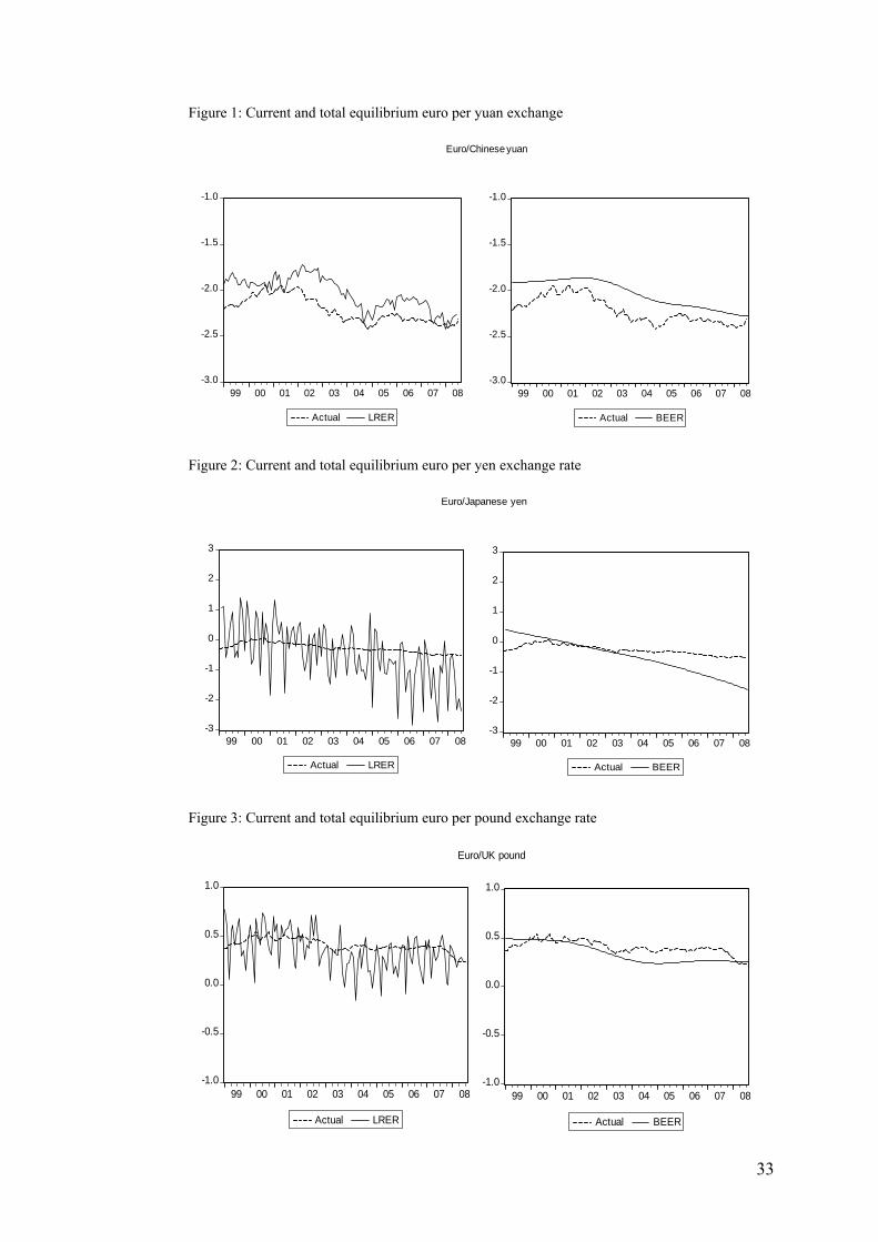
33

Figure 1: Current and total equilibrium euro per yuan exchange

-3.0

-2.5

-2.0

-1.5

-1.0

99 00 01 02 03 04 05 06 07 08

Actual BEER

-3.0

-2.5

-2.0

-1.5

-1.0

99 00 01 02 03 04 05 06 07 08

Actual LRER

Euro/Chinese yuan

Figure 2: Current and total equilibrium euro per yen exchange rate

-3

-2

-1

0

1

2

3

99 00 01 02 03 04 05 06 07 08

Actual LRER

-3

-2

-1

0

1

2

3

99 00 01 02 03 04 05 06 07 08

Actual BEER

Euro/Japanese yen

Figure 3: Current and total equilibrium euro per pound exchange rate

-1.0

-0.5

0.0

0.5

1.0

99 00 01 02 03 04 05 06 07 08

Actual BEER

-1.0

-0.5

0.0

0.5

1.0

99 00 01 02 03 04 05 06 07 08

Actual LRER

Euro/UK pound

34

Figure 4: Current and total equilibrium euro per dollar exchange rate

-1.0

-0.5

0.0

0.5

1.0

99 00 01 02 03 04 05 06 07 08

Actual BEER

-1.0

-0.5

0.0

0.5

1.0

99 00 01 02 03 04 05 06 07 08

Actual LRER

Euro/US dollar

35

Table 1: Description of data

Country

Exchange rate (euro against

foreign currency)

Consumer price index

Money supply

Industrial production

Euro area 64H M2 (59MBU) 66 China WE 64 M2 (59MB) 66 Japan AE 64 M2 (59MBA) 66 UK AG 64H M4a 66 USA AE 64 M2 (59MB) 66 All data were obtained from the International Financial Statistics (IFS) of the International Monetary Fund. The entry in each cell refers to the line of the IFS database. a M4 for the UK was obtained from the Bank of England. For China and Japan the IFS data series report the nominal exchange rates against the US dollar. To obtain the nominal exchange rates against the euro, we used cross exchange rates. The time span is 1999:01-2008:08.

36

Table 2: Two-break LM unit root test results

Variables Model k̂

B̂T 1 2ˆ ˆ,λ λ LM

Euro area/ China

s (y-y*)

(m-m*) (π-π*)

A A A A

11 12 12 11

2004:10, 2006:04 2001:11n, 2003:01

2001:05, 2007:01 2001:11, 2004:11

NA NA NA NA

-2.36 -2.72 -2.61 -3.95*

Euro area/ Japan

s (y-y*)

(m-m*) (π-π*)

A A A A

7 12 12 11

2000:07, 2001:04 2000:09, 2003:01n

2001:01, 2002:02n

2000:04n, 2000:07

NA NA NA NA

-2.80 -3.15 -2.57 -3.38

Euro area/ UK

s (y-y*)

(m-m*) (π-π*)

C C C C

11 11 12 11

2002:12, 2006:08 2000:05, 2003:10 2002:12, 2006:04 2000:06, 2001:07

0.2, 0.8 0.2, 0.6 0.2, 0.8 0.2, 0.4

-4.69 -6.54**-5.06

-7.05**Euro area/ USA

s (y-y*)

(m-m*) (π-π*)

C C C C

11 12 12 12

2002:03, 2005:03 2000:09, 2005:05 2000:12n, 2003:112000:10, 2005:11

0.2, 0.8 0.2, 0.8 0.4, 0.6 0.2, 0.8

-4.43 -4.18 -4.89

-7.73**Model A Model C

Critical values Break points Critical values 1% 5% 10% ( )1 2,λ λ λ= 1% 5% 10%

-4.54 -3.84 -3.50 λ=(0.2, 0.4) λ=(0.2, 0.6) λ=(0.2, 0.8) λ=(0.4, 0.6)

-6.16 -6.41 -6.33 -6.45

-5.59 -5.74 -5.71 -5.67

-5.27 -5.32 -5.33 -5.31

s is the natural logarithm of the nominal exchange rate of the euro against the foreign currency; y is the natural logarithm of the industrial production, m is the natural logarithm of the money supply and π is the inflation rate. k̂ is the estimated number of lags in the unit root test regression (17) to correct for serial correlation. B̂T denotes the estimated break points. 1̂λ and 2̂λ are the estimated relative break points. NA means ‘‘not affected” by the break points. The critical values for Models A and C are from table 2 of Lee and Strazicich (2003). n signifies that the relevant break is not significant at the 0.10 level of significance. ** (*) denotes rejection of the unit root hypothesis at the 0.01 (0.05) level of significance.

37

Table 3: One-break LM unit root test results

Variables Model k̂

B̂T λ̂ LM

Euro area/ China

(y-y*) A 12 2003:01 NA -2.29

Euro area/ Japan

(y-y*) (m-m*) (π-π*)

A A A

12 12 12

2000:09 2001:01 2000:07

NA NA NA

-3.11 -2.52 -3.17

Euro area/ USA

(m-m*)

C 12 2003:07 0.5 -3.30

Model A Model C Critical values Break points Critical values

1% 5% 10% λ 1% 5% 10% -4.24 -3.57 -3.21 λ=0.5 -5.11 -4.51 -4.17

m is the natural logarithm of the money supply. k̂ is the estimated number of lags in the unit root test regression (17) to correct for serial correlation. B̂T denotes the estimated break points. λ̂ is the estimated relative break point. NA means ‘‘not affected” by the break points. The critical values for Models A and C are from table 1 of Lee and Strazicich (2004). n signifies that the relevant break is not significant at the 0.10 level of significance.

38

Table 4: The JMN and LST cointegration tests with structural breaks

Country ( )0p r− ( )0JMNLR r ( )0LSTLR r p-values JMN

p-values LST

k̂

Euro area/ China

4 3 2 1

95.41** 56.76* 29.82 11.40

48.62** 17.62 4.50 0.04

0.006 0.079 0.248 0.408

0.022 0.580 0.910 0.998

3

Euro area/ Japan

4 3 2 1

164.73** 102.79** 46.65** 14.10

54.55** 20.61 11.31 0.32

0.000 0.000 0.002 0.172

0.004 0.354 0.256 0.960

5

Euro area/ UK

4 3 2 1

110.32** 59.58** 32.88** 10.12

64.77** 24.83 8.58 0.35

0.000 0.001 0.022 0.327

0.004 0.511 0.881 0.999

5

Euro area/ USA

4 3 2 1

120.36** 66.28 37.04 13.75

53.78* 31.55 15.08 2.38

0.003 0.203 0.384 0.626

0.060 0.176 0.382 0.910

9

k̂ denotes the estimated lag length in the VECM. ** and * denote rejection of the null hypothesis at the 0.05 and the 0.10 level of significance, respectively.

39

Table 5: Estimated coefficients of the cointegrating vectors

Parameter estimates

Euro area/ China

Euro area/ Japan

Euro area/ UK

Euro area/ USA

Sβ 1.000 1.000 1.000 1.000

( )*y yβ − 0.049 (0.147) [0.702]

-4.163** (7.253) [0.007]

3.618** (26.647) [0.000]

-0.157 (0.029) [0.865]

( )*m mβ − 2.032** (36.999) [0.000]

2.328 (2.225) [0.136]

-0.116** (198.692)

[0.000]

-1.050** (4.908) [0.027]

( )*π πβ − 0.066** (18.455) [0.000]

2.015** (67.123) [0.000]

-0.065 (0.273) [0.601]

0.559** (14.026) [0.000]

Trend 0.018** (16.799) [0.000]

-0.019** (5.302) [0.021]

-0.007** (14.936) [0.000]

-0.003* (2.933) [0.087]

1SB -0.313** (10.506) [0.001]

0.136 (1.098) [0.295]

-0.002* (2.769) [0.096]

-0.003 (2.325) [0.127]

2SB -0.327** (6.723) [0.009]

0.443** (4.049) [0.044]

-0.002 (2.545) [0.111]

-0.002 (0.997) [0.318]

' sβ are the parameters of the cointegrating vectors, normalized on the nominal exchange rate, 1SB is the first structural break and 2SB is the second structural break. Numbers in parentheses are likelihood ratio statistics for 0 : 0iH β = , 0 : 0H trend = or

0 : 0iH SB = and numbers in brackets are the respective p-values. For the Euro area/UK and Euro area/USA cases the structural breaks are trend breaks, while for the Euro area/China and Euro area/Japan cases the structural breaks are breaks in the constant term. ** (*) denotes rejection of the null hypothesis at the 0.05 (0.10) level of significance.

40

Table 6: Adjustment coefficients and weak exogeneity tests

Parameter estimates

Euro area/ China

Euro area/ Japan

Euro area/ UK

Euro area/ USA

Sα -0.006 (0.172) [0.679]

-0.011 (0.770) [0.380]

-0.026 (0.756) [0.385]

-0.251** (22.650) [0.000]

( )*y yα − 0.029 (0.036) [0.851]

-0.076** (16.216) [0.000]

0.414** (23.465) [0.000]

0.001 (0.003) [0.955]

( )*m mα − 0.034** (41.405) [0.000]

0.007** (7.568) [0.006]

-0.004 (0.111) [0.739]

-0.036** (9.016) [0.003]

( )*π πα − 1.481** (17.848) [0.000]

0.981** (43.113) [0.000]

0.238 (0.339) [0.560]

2.157** (11.425) [0.000]

' sα are the adjustment coefficients. Numbers in parentheses are likelihood ratio statistics for 0 : 0iH α = and numbers in brackets are the respective p-values. ** (*) denotes rejection of the null hypothesis at the 0.05 (0.10) level of significance.