Bayesian Learning (Part I) · Introduction Background Features of Bayesian Learning Methods 1...
48
Bayesian Learning (Part I) Machine Learning 6.1 - 6.6 Richard McAllister March 31, 2008 1 / 47
Transcript of Bayesian Learning (Part I) · Introduction Background Features of Bayesian Learning Methods 1...
Bayesian Learning (Part I)Machine Learning 6.1 - 6.6
Richard McAllister
March 31, 2008
1 / 47
Outline
1 IntroductionBackground
2 Bayes Theorem
3 Bayes Theorem and Concept LearningBrute-Force Bayes Concept LearningMAP Hypotheses and Consistent Learners
4 Maximum Likelihood and Least-Squared Error Hypotheses
5 Maximum Likelihood Hypotheses for Predicting ProbabilitiesGradient Search to Maximize Likelihood in a Neural Net
6 Minimum Description Length Principle
2 / 47
Introduction
Overview
We can assume that quantities of interest are governed byprobability distributions.Quantitative approach.Learning through direct manipulation of probabilities.Framework for analysis of other algorithms.
3 / 47
Introduction Background
What are Bayesian learning methods doing in this book?
1 Bayesian learning algorithms are among the most practicalapproaches to certain types of learning problems.
2 Bayesian methods aid in understanding other learning algorithms.
4 / 47
Introduction Background
Features of Bayesian Learning Methods
1 Training examples have an incremental effect on estimatedprobabilities of hypothesis correctness.
2 Prior knowledge and observed data combined to determineprobabilities of hypotheses.
3 Hypotheses can make probabilistic predictions.4 Combinations of multiple hypotheses can classify new instances.5 Other methods can be measured vis a vis optimality against
Bayesian methods.
5 / 47

Bayes Theorem
The heart of the matter:
What does it mean to have the "best" hypothesis?
6 / 47
Bayes Theorem
An answer:
best hypothesis = most probable hypothesis
7 / 47
Bayes Theorem
Some notation:
D: the training dataH: the set of all hypothesesh: a hypothesis h ∈ HP(h): the prior probability of h: the initial probability thathypothesis h holds, before we have observed the training dataP(D): the prior probability that training data D will be observedP(D | h): the probability of observing data D given some world inwhich h holdsP(x | y): the probability of x occurring given that y has beenobservedP(h | D): the posterior probability of h given D: the probability thath holds given the observed training data D
8 / 47
Bayes Theorem
Bayes Theorem:
P(h | D) = P(D|h)P(h)P(D)
This means: the posterior probability of D given h equals theprobability of observing data D given some world in which h holdstimes the prior probability of h all over the prior probability of D.
9 / 47
Bayes Theorem
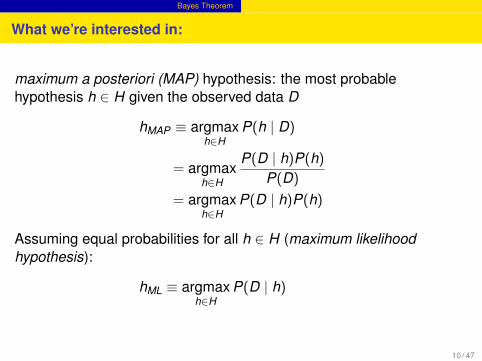
What we’re interested in:
maximum a posteriori (MAP) hypothesis: the most probablehypothesis h ∈ H given the observed data D
hMAP ≡ argmaxh∈H
P(h | D)
= argmaxh∈H
P(D | h)P(h)
P(D)
= argmaxh∈H
P(D | h)P(h)
Assuming equal probabilities for all h ∈ H (maximum likelihoodhypothesis):
hML ≡ argmaxh∈H
P(D | h)
10 / 47
Bayes Theorem
Where does Bayes theorem work?
Any set H of mutually exclusive propositions whose probabilities sumto one.
11 / 47

Bayes Theorem
An example:
A grim scenario at the doctor’s office:1 a patient has cancer2 the patient does not have cancer
12 / 47
Bayes Theorem
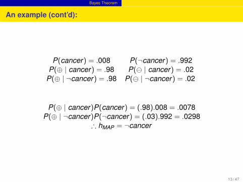
An example (cont’d):
P(cancer) = .008 P(¬cancer) = .992P(⊕ | cancer) = .98 P( | cancer) = .02
P(⊕ | ¬cancer) = .98 P( | ¬cancer) = .02
P(⊕ | cancer)P(cancer) = (.98).008 = .0078P(⊕ | ¬cancer)P(¬cancer) = (.03).992 = .0298
∴ hMAP = ¬cancer
13 / 47
Bayes Theorem
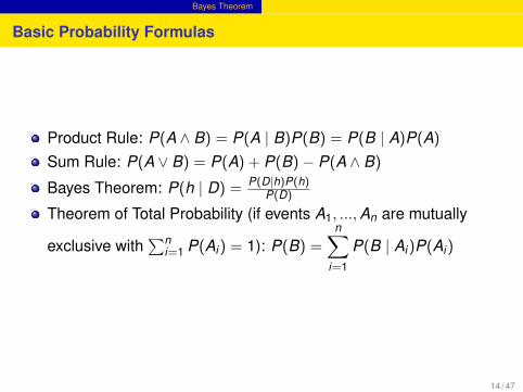
Basic Probability Formulas
Product Rule: P(A ∧ B) = P(A | B)P(B) = P(B | A)P(A)
Sum Rule: P(A ∨ B) = P(A) + P(B)− P(A ∧ B)
Bayes Theorem: P(h | D) = P(D|h)P(h)P(D)
Theorem of Total Probability (if events A1, ...,An are mutually
exclusive with∑n
i=1 P(Ai) = 1): P(B) =n∑
i=1
P(B | Ai)P(Ai)
14 / 47
Bayes Theorem and Concept Learning
The Big Idea
"Since Bayes theorem provides a principled way to calculate theposterior probability of each hypothesis given the training data, we canuse it as the basis for a straightforward learning algorithm thatcalculates the probability for each possible hypothesis, then outputsthe most probable."(ML pg 158)
15 / 47
Bayes Theorem and Concept Learning Brute-Force Bayes Concept Learning
More Terminology (Ugh!)
X : the instance spacexi : some instance from XD: the training datadi : the target value of xi
c: the target concept (c : X → {0,1} and di = c(xi))〈x1 . . . xm〉: the sequence of instances〈d1 . . . dm〉: the sequence of target values
16 / 47
Bayes Theorem and Concept Learning Brute-Force Bayes Concept Learning
Brute-Force MAP Learning
Two steps:1 For each h in H, calculate the posterior probability:
P(h | D) = P(D|h)P(h)P(D)
2 Output hMAP
hMAP ≡ argmaxh∈H
P(h | D)
Note: Since each h ∈ H is calculated, it’s possible that a lot ofcalculation must be done here.
17 / 47
Bayes Theorem and Concept Learning Brute-Force Bayes Concept Learning
Constraining Our Example
We have some flexibility in how we may choose probability distributionsP(h) and P(D | h). The following assumptions have been made:
1 The training data D is noise free (i.e., di = c(xi))2 The target concept c is contained in the hypothesis space H.3 We have no a priori reason to believe that any hypothesis is more
probable than any other.
18 / 47
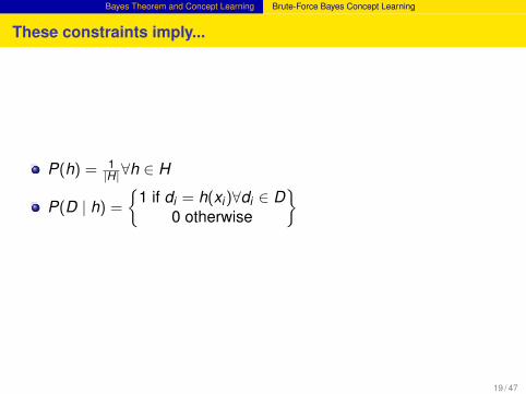
Bayes Theorem and Concept Learning Brute-Force Bayes Concept Learning
These constraints imply...
P(h) = 1|H|∀h ∈ H
P(D | h) =
{1 if di = h(xi)∀di ∈ D
0 otherwise
}
19 / 47
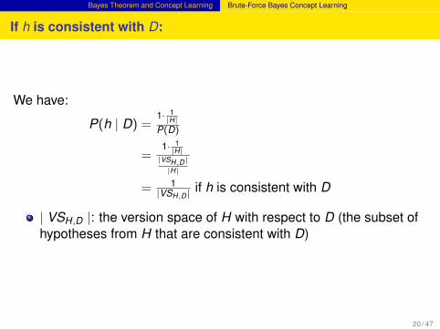
Bayes Theorem and Concept Learning Brute-Force Bayes Concept Learning
If h is consistent with D:
We have:
P(h | D) =1· 1
|H|P(D)
=1· 1
|H||VSH,D |
|H|
= 1|VSH,D | if h is consistent with D
| VSH,D |: the version space of H with respect to D (the subset ofhypotheses from H that are consistent with D)
20 / 47
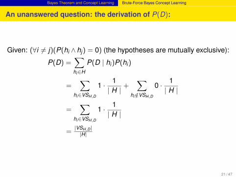
Bayes Theorem and Concept Learning Brute-Force Bayes Concept Learning
An unanswered question: the derivation of P(D):
Given: (∀i 6= j)(P(hi ∧ hj) = 0) (the hypotheses are mutually exclusive):
P(D) =∑hi∈H
P(D | hi)P(hi)
=∑
hi∈VSH,D
1 · 1| H |
+∑
hi /∈VSH,D
0 · 1| H |
=∑
hi∈VSH,D
1 · 1| H |
=|VSH,D ||H|
21 / 47
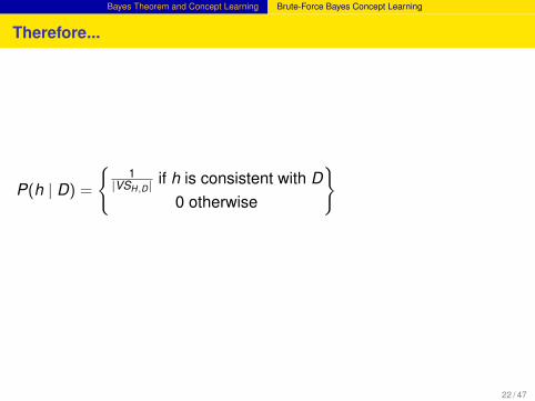
Bayes Theorem and Concept Learning Brute-Force Bayes Concept Learning
Therefore...
P(h | D) =
{1
|VSH,D | if h is consistent with D0 otherwise
}
22 / 47
Bayes Theorem and Concept Learning Brute-Force Bayes Concept Learning
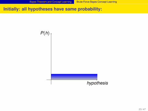
Initially: all hypotheses have same probability:
hypothesis
P(h)
23 / 47
Bayes Theorem and Concept Learning Brute-Force Bayes Concept Learning
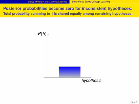
Posterior probabilities become zero for inconsistent hypotheses:Total probability summing to 1 is shared equally among remaining hypotheses:
hypothesis
P(h)
24 / 47
Bayes Theorem and Concept Learning Brute-Force Bayes Concept Learning
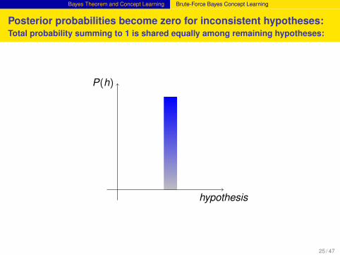
Posterior probabilities become zero for inconsistent hypotheses:Total probability summing to 1 is shared equally among remaining hypotheses:
hypothesis
P(h)
25 / 47
Bayes Theorem and Concept Learning MAP Hypotheses and Consistent Learners
Consistent Learners
consistent learner: a learning algorithm that outputs a hypothesisthat commits zero errors over the training examples.
Every consistent learner outputs a MAP hypothesis if we assume:uniform prior probability distribution over Hdeterministic, noise-free training data
Example: Find-S outputs the maximally specific consistent hypothesis,which is a MAP hypothesis.
26 / 47
Bayes Theorem and Concept Learning MAP Hypotheses and Consistent Learners
Characterizing the Behavior of Learning Algorithms
Recall: the inductive bias of a learning algorithm is the set ofassumptions B sufficient to deductively justify the inductive inferenceperformed by the learner.
inductive inference can also be modeled using probabilisticreasoning based on Bayes theorem.assumptions are of the form: "the prior probabilities over H aregiven by the distribution P(h), and the strength of data in rejectingor accepting a hypothesis is given by P(D | h)."P(h) and P(D | h) characterize the implicit assumptions of thealgorithms being studied:
Candidate-EliminationFind-S
P(D | h) can also take on values other than 0 or 1.
27 / 47
Maximum Likelihood and Least-Squared Error Hypotheses
Premise: "...under certain assumptions any learning algorithm thatminimizes the squared error between the output hypothesis predictionsand the training data will output a maximum likelihood hypothesis." (pg.164)
neural networks do thisso do other curve fitting methods
28 / 47
Maximum Likelihood and Least-Squared Error Hypotheses
More Terminology
probability density function: p(x0) ≡ limε→0
1ε
P(x0 ≤ x < x0 + ε)
e: a random noise variable generated by a Normal probabilitydistribution〈x1 . . . xm〉: the sequence of instances (as before)〈d1 . . . dm〉: the sequence of target values with di = f (xi) + ei
29 / 47
Maximum Likelihood and Least-Squared Error Hypotheses
We wish to show that...
...the least-squared error hypothesis is, in fact, the maximum likelihoodhypothesis (within our problem setting).
Using the previous definition of hML we have: argmaxh∈H
p(D | h)
Assuming training examples are mutually independent given h:
hML = argmaxh∈H
m∏i=1
p(di | h)
Since ei follows a Normal distribution, di must also follow thesame. Therefore:
p(di | h) = 1√2πσ2 e−
12α2 (di−µ)2
with mean µ and variance σ2
30 / 47
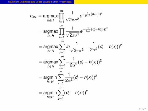
Maximum Likelihood and Least-Squared Error Hypotheses
hML = argmaxh∈H
m∏i=1
1√2πσ2
e−1
2α2 (di−µ)2
= argmaxh∈H
m∏i=1
1√2πσ2
e−1
2α2 (di−h(xi ))2
= argmaxh∈H
m∑i=1
ln1√
2πσ2− 1
2α2 (di − h(xi))2
= argmaxh∈H
m∑i=1
− 12α2 (di − h(xi))2
= argminh∈H
m∑i=1
12α2 (di − h(xi))2
= argminh∈H
m∑i=1
(di − h(xi))2
31 / 47
Maximum Likelihood and Least-Squared Error Hypotheses
Therefore...
The maximum likelihood hypothesis hML is the one that minimizes thesum of the squared errors between the observed training values di andthe hypothesis predictions h(xi).
32 / 47
Maximum Likelihood Hypotheses for Predicting Probabilities
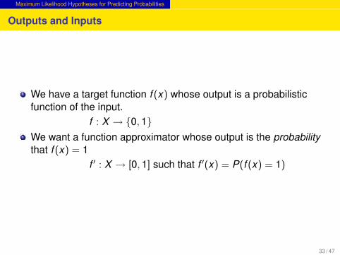
Outputs and Inputs
We have a target function f (x) whose output is a probabilisticfunction of the input.
f : X → {0,1}We want a function approximator whose output is the probabilitythat f (x) = 1
f ′ : X → [0,1] such that f ′(x) = P(f (x) = 1)
33 / 47
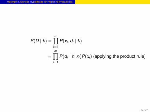
Maximum Likelihood Hypotheses for Predicting Probabilities
P(D | h) =m∏
i=1
P(xi ,di | h)
=m∏
i=1
P(di | h, xi)P(xi) (applying the product rule)
34 / 47
Maximum Likelihood Hypotheses for Predicting Probabilities
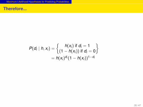
Therefore...
P(di | h, xi) =
{h(xi) if di = 1
(1− h(xi)) if di = 0
}= h(xi)
di (1− h(xi))1−di
35 / 47
Maximum Likelihood Hypotheses for Predicting Probabilities
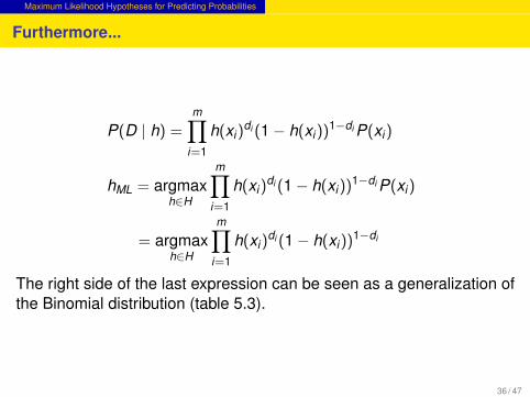
Furthermore...
P(D | h) =m∏
i=1
h(xi)di (1− h(xi))1−di P(xi)
hML = argmaxh∈H
m∏i=1
h(xi)di (1− h(xi))1−di P(xi)
= argmaxh∈H
m∏i=1
h(xi)di (1− h(xi))1−di
The right side of the last expression can be seen as a generalization ofthe Binomial distribution (table 5.3).
36 / 47
Maximum Likelihood Hypotheses for Predicting Probabilities
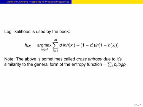
Log likelihood is used by the book:
hML = argmaxh∈H
m∑i=1
di lnh(xi) + (1− di)ln(1− h(xi))
Note: The above is sometimes called cross entropy due to it’ssimilarity to the general form of the entropy function −
∑i pi logpi
37 / 47
Maximum Likelihood Hypotheses for Predicting Probabilities Gradient Search to Maximize Likelihood in a Neural Net
What we want:
We desire a weight-training rule for neural network learning thatseeks to maximize the maximum likelihood hypothesis (G(h,D))using gradient ascent.
38 / 47
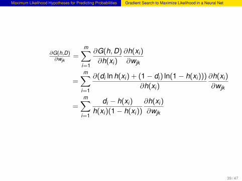
Maximum Likelihood Hypotheses for Predicting Probabilities Gradient Search to Maximize Likelihood in a Neural Net
∂G(h,D)∂wjk
=m∑
i=1
∂G(h,D)
∂h(xi)
∂h(xi)
∂wjk
=m∑
i=1
∂(di ln h(xi) + (1− di) ln(1− h(xi)))
∂h(xi)
∂h(xi)
∂wjk
=m∑
i=1
di − h(xi)
h(xi)(1− h(xi))
∂h(xi)
∂wjk
39 / 47
Maximum Likelihood Hypotheses for Predicting Probabilities Gradient Search to Maximize Likelihood in a Neural Net
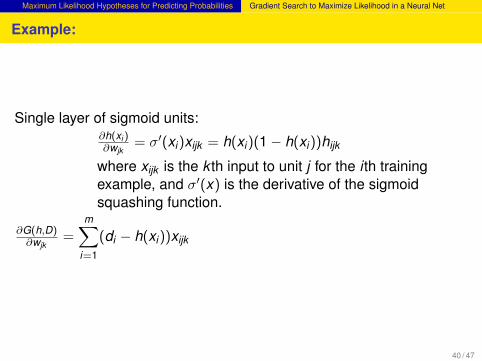
Example:
Single layer of sigmoid units:∂h(xi )∂wjk
= σ′(xi)xijk = h(xi)(1− h(xi))hijk
where xijk is the k th input to unit j for the i th trainingexample, and σ′(x) is the derivative of the sigmoidsquashing function.
∂G(h,D)∂wjk
=m∑
i=1
(di − h(xi))xijk
40 / 47
Maximum Likelihood Hypotheses for Predicting Probabilities Gradient Search to Maximize Likelihood in a Neural Net
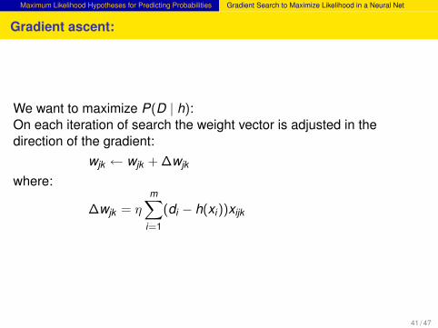
Gradient ascent:
We want to maximize P(D | h):On each iteration of search the weight vector is adjusted in thedirection of the gradient:
wjk ← wjk + ∆wjk
where:
∆wjk = η
m∑i=1
(di − h(xi))xijk
41 / 47
Maximum Likelihood Hypotheses for Predicting Probabilities Gradient Search to Maximize Likelihood in a Neural Net
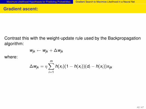
Gradient ascent:
Contrast this with the weight-update rule used by the Backpropagationalgorithm:
wjk ← wjk + ∆wjk
where:
∆wjk = η
m∑i=1
h(xi)(1− h(xi))(di − h(xi))xijk
42 / 47
Minimum Description Length Principle
What the is the Minimum Description Length Principle?
A Bayesian perspective on Occam’s razorMotivated by interpreting the definition of hMAP in the light of basicconcepts from information theory.
43 / 47
Minimum Description Length Principle
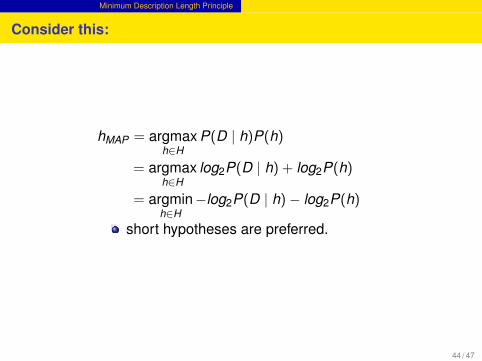
Consider this:
hMAP = argmaxh∈H
P(D | h)P(h)
= argmaxh∈H
log2P(D | h) + log2P(h)
= argminh∈H
−log2P(D | h)− log2P(h)
short hypotheses are preferred.
44 / 47
Minimum Description Length Principle
Terminology
C: the code used to encode a messagei : the messageLC(i): the description length of message i with respect to C...ormore simply, the number of bits used to encode the message
45 / 47
Minimum Description Length Principle
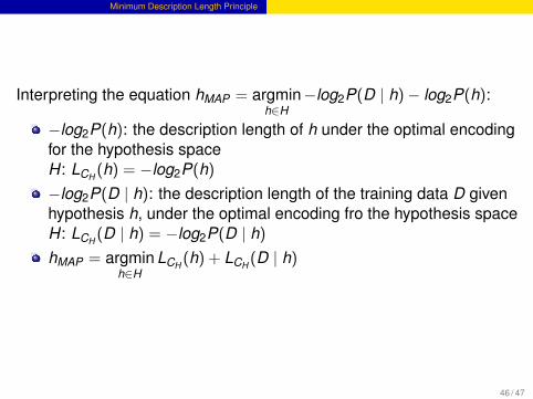
Interpreting the equation hMAP = argminh∈H
−log2P(D | h)− log2P(h):
−log2P(h): the description length of h under the optimal encodingfor the hypothesis spaceH: LCH (h) = −log2P(h)
−log2P(D | h): the description length of the training data D givenhypothesis h, under the optimal encoding fro the hypothesis spaceH: LCH (D | h) = −log2P(D | h)
hMAP = argminh∈H
LCH (h) + LCH (D | h)
46 / 47
Minimum Description Length Principle
Minimum Description Length Principle:
Choose hMDL where:hMDL = argmin
h∈HLC1(h) + LC1(D | h)
provides a way of trading off hypothesis complexity for the numberof errors committed by the hypothesis.provides a way to deal with the issue of overfitting the data.short imperfect hypothesis may be selected over a long perfecthypothesis.
47 / 47

Minimum Description Length Principle
Thank you!
48 / 47