Bayesian Inference in Processing Experimental Data

Principles and Basic Applications

G. D’AgostiniUniversita “La Sapienza” and INFN, Roma, Italia

Abstract

This report introduces general ideas and some basic methods of the Bayesian probabilitytheory applied to physics measurements. Our aim is to make the reader familiar, through ex-amples rather than rigorous formalism, with concepts such as: model comparison (includingthe automatic Ockham’s Razor filter provided by the Bayesian approach); parametric infer-ence; quantification of the uncertainty about the value of physical quantities, also takinginto account systematic effects; role of marginalization; posterior characterization; predic-tive distributions; hierarchical modelling and hyperparameters; Gaussian approximation ofthe posterior and recovery of conventional methods, especially maximum likelihood and chi-square fits under well defined conditions; conjugate priors, transformation invariance andmaximum entropy motivated priors; Monte Carlo estimates of expectation, including a shortintroduction to Markov Chain Monte Carlo methods. 0

1 Introduction

The last decades of 20th century have seen an intense expansion in the use of Bayesian methods inall fields of human activity that generally deal with uncertainty, including engineering, computerscience, economics, medicine and even forensics (Kadane and Schum 1996). Bayesian networks(Pearl 1988, Cowell et al 1999) are used to diagrammatically represent uncertainty in expertsystems or to construct artificial intelligence systems. Even venerable metrological associations,such as the International Organization for Standardization (ISO 1993), the Deutsches Institutfur Normung (DIN 1996, 1999), and the USA National Institute of Standards and Technology(Taylor and Kuyatt 1994), have come to realize that Bayesian ideas are essential to providegeneral methods for quantifying uncertainty in measurements. A short account of the Bayesianupsurge can be found in a Science article (Malakoff 1999). A search on the web for the keywords‘Bayesian,’ ‘Bayesian network,’ or ‘belief network’ gives one a dramatic impression of this ‘rev-olution,’ not only in terms of improved methods, but more importantly in terms of reasoning.An overview of recent developments in Bayesian statistics, may be found in the proceedings ofthe Valencia Conference series. The last published volume was (Bernardo et al 1999), and themost recent conference was held in June 2002. Another series of workshops, under the titleof Maximum Entropy and Bayesian Methods, has focused more on applications in the physicalsciences.

It is surprising that many physicists have been slow to adopt these ‘new’ ideas. There havebeen notable exceptions, of course, many of whom have contributed to the abovementionedMaximum Entropy workshops. One reason to be surprised is because numerous great physicistsand mathematicians have played important roles in developing probability theory. These ‘new’ideas actually originated long ago with Bernoulli, Laplace, and Gauss, just to mention a few

0Invited article to be published in Reports on Progress in Physics.Email: dagostini@roma1.infn.it, URL: http://www.roma1.infn.it/ dagos.

1

who contributed significantly to the development of physics, as well as to Bayesian thinking.So, while modern statisticians and mathematicians are developing powerful methods to applyto Bayesian analysis, most physicists, in their use and reasoning in statistics still rely on 20th

century ‘frequentist prescriptions’ (D’Agostini 1999a, 2000).We hope that this report will help fill this gap by reviewing the advantages of using the

Bayesian approach to address physics problems. We will emphasize more the intuitive andpractical aspects than the theoretical ones. We will not try to cover all possible applications ofBayesian analysis in physics, but mainly concentrate on some basic applications that illustrateclearly the power of the method and how naturally it meshes with physicists’ approach to theirscience.

The vocabulary, expressions, and examples have been chosen with the intent to correspond,as closely as possible, to the education that physicists receive in statistics, instead of a morerigorous approach that formal Bayesian statisticians might prefer. For example, we avoid manyimportant theoretical concepts, like exchangeability, and do not attempt to prove the basic rulesof probability. When we talk about ‘random variables,’ we will in fact mean ‘uncertain variables,’and instead of referring to the frequentist concept of ‘randomness’ a la von Mises (1957). Thisdistinction will be clarified later.

In the past, presentations on Bayesian probability theory often start with criticisms of ‘con-ventional,’ that is, frequentist ideas, methods, and results. We shall keep criticisms and detailedcomparisons of the results of different methods to a minimum. Readers interested in a criticalreview of conventional frequentist statistics will find a large literature, because most introduc-tory books or reports on Bayesian analysis contain enough material on this matter. See (Gelmanet al 1995, Sivia 1997, D’Agostini 1999c, Jaynes 1998, Loredo 1990) and the references therein.Eloquent ‘defenses of the Bayesian choice’ can be found in (Howson and Urbach 1993, Robert2001).

Some readers may wish to have references to unbiased comparisons of frequentist to Bayesianideas and methods. To our knowledge, no such reports exist. Those who claim to be impartialare often frequentists who take some Bayesian results as if they were frequentist ‘prescriptions,’not caring whether all underlying hypotheses apply. For two prominent papers of this kind,see the articles by Efron (1986a) [with follow up discussions by Lindley (1989), Zellner (1986),and Efron (1986b)] and Cousins (1995). A recent, pragmatic comparisons of frequentist andBayesian confidence limits can be found in (Zech 2002).

Despite its lack of wide-spread use in physics, and its complete absence in physics courses(D’Agostini 1999a), Bayesian data analysis is increasingly being employed in many areas ofphysics, for example, in astronomy (Gregory and Loredo 1992, 1996, Gregory 1999, Babu andFeigelson 1992, 1997, Bontekoe et al 1994), in geophysics (Glimm and Sharp 1999), in high-energy physics (D’Agostini and Degrassi 1999, Ciuchini et al 2001), in image reconstruction(Hanson 1993), in microscopy (Higdon and Yamamoto 2001), in quantum Monte Carlo (Guber-natis et al 1991), and in spectroscopy (Skilling 1992, Fischer et al 1997, 1998, 2000), just tomention a few articles written in the last decade. Other examples will be cited throughout thepaper.

2 Uncertainty and probability

In the practice of science, we constantly find ourselves in a state of uncertainty. Uncertaintyabout the data that an experiment shall yield. Uncertainty about the true value of a physicalquantity, even after an experiment has been done. Uncertainty about model parameters, cali-bration constants, and other quantities that might influence the outcome of the experiment, andhence influence our conclusions about the quantities of interest, or the models that might haveproduced the observed results.

2

In general, we know through experience that not all the events that could happen, or allconceivable hypotheses, are equally likely. Let us consider the outcome of you measuring thetemperature at the location where you are presently reading this paper, assuming you use adigital thermometer with one degree resolution (or you round the reading at the degree if youhave a more precise instrument). There are some values of the thermometer display you aremore confident to read, others you expect less, and extremes you do not believe at all (someof them are simply excluded by the thermometer you are going to use). Given two events E1

and E2, for example E1 : “T = 22C” and E2 : “T = 33C”, you might consider E2 much moreprobable than E1, just meaning that you believe E2 to happen more than E1. We could usedifferent expressions to mean exactly the same thing: you consider E2 more likely; you are moreconfident in E2; having to choose between E1 and E2 to win a price, you would promptly chooseE2; having to classify with a number, that we shall denote with P , your degree of confidence onthe two outcomes, you would write P (E2) > P (E1); and many others.

On the other hand, we would rather state the opposite, i.e. P (E1) > P (E2), with the samemeaning of symbols and referring exactly to the same events: what you are going to read at yourplace with your thermometer. The reason is simply because we do not share the same status ofinformation. We do not know who you are and where you are in this very moment. You andwe are uncertain about the same event, but in a different way. Values that might appear veryprobable to you now, appear quite improbable, though not impossible, to us.

In this example we have introduced two crucial aspects of the Bayesian approach:

1. As it is used in everyday language, the term probability has the intuitive meaning of “thedegree of belief that an event will occur.”

2. Probability depends on our state of knowledge, which is usually different for differentpeople. In other words, probability is unavoidably subjective.

At this point, you might find all of this quite natural, and wonder why these intuitive conceptsgo by the esoteric name ‘Bayesian.’ We agree! The fact is that the main thrust of statistics theoryand practice during the 20th century has been based on a different concept of probability, inwhich it is defined as the limit of the long-term relative frequency of the outcome of these events.It revolves around the theoretical notion of infinite ensembles of ‘identical experiments.’ Withoutentering an unavoidably long critical discussion of the frequentist approach, we simply want topoint out that in such a framework, there is no way to introduce the probability of hypotheses.All practical methods to overcome this deficiency yield misleading, and even absurd, conclusions.See (D’Agostini 1999c) for several examples and also for a justification of why frequentistic test‘often work’.

Instead, if we recover the intuitive concept of probability, we are able to talk in a naturalway about the probability of any kind of event, or, extending the concept, of any proposition. Inparticular, the probability evaluation based on the relative frequency of similar events occurredin the past is easily recovered in the Bayesian theory, under precise condition of validity (seeSect. 5.3). Moreover, a simple theorem from probability theory, Bayes’ theorem, which we shallsee in the next section, allows us to update probabilities on the basis of new information. Thisinferential use of Bayes’ theorem is only possible if probability is understood in terms of degreeof belief. Therefore, the terms ‘Bayesian’ and ‘based on subjective probability’ are practicallysynonyms,and usually mean ‘in contrast to the frequentist, or conventional, statistics.’ Theterms ‘Bayesian’ and ‘subjective’ should be considered transitional. In fact, there is already thetendency among many Bayesians to simply refer to ‘probabilistic methods,’ and so on (Jeffreys1961, de Finetti 1974, Jaynes 1998 and Cowell et al 1999).

As mentioned above, Bayes’ theorem plays a fundamental role in the probability theory.This means that subjective probabilities of logically connected events are related to each other

3

by mathematical rules. This important result can be summed up by saying, in practical terms,that ‘degrees of belief follow the same grammar as abstract axiomatic probabilities.’ Hence, allformal properties and theorems from probability theory follow.

Within the Bayesian school, there is no single way to derive the basic rules of probability (notethat they are not simply taken as axioms in this approach). de Finetti’s principle of coherence(de Finetti 1974) is considered the best guidance by many leading Bayesians (Bernardo andSmith 1994, O’Hagan 1994, Lad 1996 and Coletti and Scozzafava 2002). See (D’Agostini 1999c)for an informal introduction to the concept of coherence, which in simple words can be outlinedas follows. A person who evaluates probability values should be ready to accepts bets in eitherdirection, with odd ratios calculated from those values of probability. For example, an analystthat declares to be confident 50% on E should be aware that somebody could ask him to makea 1:1 bet on E or on E. If he/she feels uneasy, it means that he/she does not consider the twoevents equally likely and the 50% was ‘incoherent.’

Others, in particular practitioners close to the Jaynes’ Maximum Entropy school (Jaynes1957a, 1957b) feel more at ease with Cox’s logical consistency reasoning, requiring some con-sistency properties (‘desiderata’) between values of probability related to logically connectedpropositions. (Cox 1946). See also (Jaynes 1998, Sivia 1997, and Frohner 2000, and especiallyTribus 1969), for accurate derivations and a clear account of the meaning and role of informationentropy in data analysis. An approach similar to Cox’s is followed by Jeffreys (1961), anotherleading figure who has contributed a new vitality to the methods based on this ‘new’ pointof view on probability. Note that Cox and Jeffreys were physicists. Remarkably, Schrodinger(1947a, 1947b) also arrived at similar conclusions, though his definition of event is closer to thede Finetti’s one. [Some short quotations from (Schrodinger 1947a) are in order. Definition ofprobability: “. . . a quantitative measure of the strength of our conjecture or anticipation, foundedon the said knowledge, that the event comes true”. Subjective nature of probability: “Since theknowledge may be different with different persons or with the same person at different times,they may anticipate the same event with more or less confidence, and thus different numericalprobabilities may be attached to the same event.” Conditional probability: “Thus whenever wespeak loosely of ‘the probability of an event,’ it is always to be understood: probability with regardto a certain given state of knowledge.”]

3 Rules of probability

We begin by stating some basic rules and general properties that form the ‘grammar’ of theprobabilistic language, which is used in Bayesian analysis. In this section, we review the rulesof probability, starting with the rules for simple propositions. We will not provide rigorousderivations and will not address the foundational or philosophical aspects of probability theory.Moreover, following an ‘eclectic’ approach which is common among Bayesian practitioners, wetalk indifferently about probability of events, probability of hypotheses or probability of propo-sitions. Indeed, the last expression will be often favoured, understanding that it does includethe others.

3.1 Probability of simple propositions

Let us start by recalling the basic rules of probability for propositions or hypotheses. Let A andB be propositions, which can take on only two values, for example, true or false. The notationP (A) stands for the probability that A is true. The elementary rules of probability for simplepropositions are

0 ≤ P (A) ≤ 1; (1)

4

P (Ω) = 1; (2)P (A ∪B) = P (A) + P (B)− P (A ∩B) . (3)P (A ∩B) = P (A |B)P (B) = P (B |A)P (A) , (4)

where Ω means tautology (a proposition that is certainly true). The construct A∩B is true onlywhen both A and B are true (logical AND), while A ∪ B is true when at least one of the twopropositions is true (logical OR). A∩B is also written simply as ‘A,B’ or AB, and is also calleda logical product, while A∪B is also called a logical sum. P (A,B) is called the joint probabilityof A and B. P (A |B) is the probability of A under that condition that B is true. We often readit simply as “the probability of A, given B.” .

Equation (4) shows that the joint probability of two events can be decomposed into con-ditional probabilities in different two ways. Either of these ways is called the product rule.If the status of B does not change the probability of A, and the other way around, then Aand B are said to be independent, probabilistically independent to be precise. In that case,P (A |B) = P (A), and P (B |A) = P (B), which, when inserted in Eq. (4), yields

P (A ∩B) = P (A)P (B) ⇐⇒ probabilistic independence . (5)

Equations (1)–(4) logically lead to other rules which form the body of probability theory. Forexample, indicating the negation (or opposite) of A with A, clearly A∪A is a tautology (A∪A =Ω), and A ∩ A is a contradiction (A ∩ A = ∅). The symbol ∅ stands for contradiction (aproposition that is certainly false). Hence, we obtain from Eqs. (2) and (3)

P (A) + P (A) = 1 , (6)

which says that proposition A is either true or not true.

3.2 Probability of complete classes

These formulae become more interesting when we consider a set of propositions Hj that alltogether form a tautology (i.e., they are exhaustive) and are mutually exclusive. Formally

∪iHj = Ω (7)Hj ∩Hk = ∅ if j 6= k . (8)

When these conditions apply, the set Hj is said to form a complete class. The symbol H hasbeen chosen because we shall soon interpret Hj as a set of hypotheses.

The first (trivial) property of a complete class is normalization, that is∑j

P (Hj) = 1 , (9)

which is just an extension of Eq. (6) to a complete class containing more than just a singleproposition and its negation.

For the complete class H, the generalizations of Eqs. (6) and the use of Eq. (4) yield:

P (A) =∑j

P (A,Hj) (10)

P (A) =∑j

P (A |Hj)P (Hj) . (11)

Equation (10) is the basis of what is called marginalization, which will become particularlyimportant when dealing with uncertain variables: the probability of A is obtained by the sum-mation over all possible constituents contained in A. Hereafter, we avoid explicitly writing the

5

limits of the summations, meaning that they extend over all elements of the class. The con-stituents are ‘A,Hj ,’ which, based on the complete class of hypotheses H, themselves forma complete class, which can be easily proved. Equation (11) shows that the probability of anyproposition is given by a weighted average of all conditional probabilities, subject to hypothesesHj forming a complete class, with the weight being the probability of the hypothesis.

In general, there are many ways to choose complete classes (like ‘bases’ in geometrical spaces).Let us denote the elements of a second complete class by Ei. The constituents are then formedby the elements (Ei,Hj) of the Cartesian product E × H. Equations (10) and (11) thenbecome the more general statements

P (Ei) =∑j

P (Ei,Hj) (12)

P (Ei) =∑j

P (Ei |Hj)P (Hj) (13)

and, symmetrically,

P (Hj) =∑

i

P (Ei,Hj) (14)

P (Hj) =∑

i

P (Hj |Ei)P (Ei) . (15)

The reason we write these formulae both ways is to stress the symmetry of Bayesian reasoningwith respect to classes E and H, though we shall soon associate them with observations (orevents) and hypotheses, respectively.

3.3 Probability rules for uncertain variables

In analyzing the data from physics experiments, we need to deal with measurement that arediscrete or continuous in nature. Our aim is to make inferences about the models that we believeappropriately describe the physical situation, and/or, within a given model, to determine thevalues of relevant physics quantities. Thus, we need the probability rules that apply to uncertainvariables, whether they are discrete or continuous. The rules for complete classes described inthe preceding section clearly apply directly to discrete variables. With only slight changes, thesame rules also apply to continuous variables because they may be thought of as a limit ofdiscrete variables, as interval between possible discrete values goes to zero.

For a discrete variable x, the expression p(x), which is called a probability function, hasthe interpretation in terms of the probability of the proposition P (A), where A is true whenthe value of the variable is equal to x. In the case of continuous variables, we use the samenotation, but with the meaning of a probability density function (pdf). So p(x) dx, in terms ofa proposition, is the probability P (A), where A is true when the value of the variable lies inthe range of x to x + dx. In general, the meaning is clear from the context; otherwise it shouldbe stated. Probabilities involving more than one variable, like p(x, y), have the meaning of theprobability of a logical product; they are usually called joint probabilities.

Table 1 summarizes useful formulae for discrete and continuous variables. The interpretationand use of these relations in Bayesian inference will be illustrated in the following sections.

4 Bayesian inference for simple problems

We introduce the basic concepts of Bayesian inference by considering some simple problems.The aim is to illustrate some of the notions that form the foundation of Bayesian reasoning.

6

Table 1: Some definitions and properties of probability functions for values of a discrete variablexi and probability density functions for continuous variables x. All summations and integralsare understood to extend over the full range of possibilities of the variable. Note that theexpectation of the variable is also called expected value (sometimes expectation value), averageand mean. The square root of the variance is the standard deviation σ.

discrete variables continuous variables

probability P (X = xi) = p(xi) dP[x≤X≤x+dx] = p(x) dx

normalization†∑

i p(xi) = 1∫p(x) dx = 1

expectation of f(X) E[f(X)] =∑

i f(xi) p(xi) E[f(X)] =∫f(x) p(x) dx

expected value E(X) =∑

i xi p(xi) E(X) =∫x p(x) dx

moment of order r Mr(X) =∑

i xri p(xi) Mr(X) =

∫xr p(x) dx

variance σ2 =∑

i[xi − E(X)]2 p(xi) σ2 =∫[x− E(X)]2 p(x) dx

product rule p(xi, yj) = p(xi | yj) p(yj) p(x, y) = p(x | y) p(y)

independence p(xi, yj) = p(xi) p(yj) p(x, y) = p(x) p(y)

marginalization∑

j p(xi, yj) = p(xi)∫p(x, y) dy = p(x)

decomposition p(xi) =∑

j p(xi |yj) p(yj) p(x) =∫p(x | y) p(y) dy

Bayes’ theorem p(xj | yi) = p(yi |xj) p(xj)∑j p(yi |xj) p(xj)

p(x | y) = p(y |x) p(x)∫p(y |x) p(x) dx

likelihood L(xj ; yi) = p(yi |xj) L(x ; y) = p(y |x)

†A function p(x) such that∑

ip(xi) =∞, or

∫p(x) dx =∞, is called improper. Improper

functions are often used to describe relative beliefs about the possible values of a variable.

7

4.1 Background information

As we think about drawing conclusions about the physical world, we come to realize that ev-erything we do is based on what we know about the world. Conclusions about hypotheses willbe based on our general background knowledge. To emphasize the dependence of probability onthe state of background information, which we designate as I, we will make it explicit by writingP (E | I), rather than simply P (E). (Note that, in general, P (A | I1) 6= P (A | I2), if I1 and I2 aredifferent states of information.) For example, Eq. (4) should be more precisely written as

P (A ∩B | I) = P (A |B ∩ I)P (B | I) = P (B |A ∩ I)P (A | I) , (16)

or alternatively as

P (A,B | I) = P (A |B, I)P (B | I) = P (B |A, I)P (A | I) . (17)

We have explicitly included I as part of the conditional to remember that any probability relationis valid only under the same state of background information.

4.2 Bayes’ theorem

Formally, Bayes’ theorem follows from the symmetry of P (A,B) expressed by Eq. (17). In termsof Ei and Hj belonging to two different complete classes, Eq. (17) yields

P (Hj |Ei, I)P (Hj | I)

=P (Ei |Hj , I)

P (Ei | I)(18)

This equation says that the new condition Ei alters our belief in Hj by the same updating factorby which the condition Hj alters our belief about Ei. Rearrangement yields Bayes’ theorem

P (Hj |Ei, I) =P (Ei |Hj , I)P (Hj | I)

P (Ei | I). (19)

We have obtained a logical rule to update our beliefs on the basis of new conditions. Note that,though Bayes’ theorem is a direct consequence of the basic rules of axiomatic probability theory,its updating power can only be fully exploited if we can treat on the same basis expressionsconcerning hypotheses and observations, causes and effects, models and data.

In most practical cases, the evaluation of P (Ei | I) can be quite difficult, while determiningthe conditional probability P (Ei |Hj, I) might be easier. For example, think of Ei as the prob-ability of observing a particular event topology in a particle physics experiment, compared withthe probability of the same thing given a value of the hypothesized particle mass (Hj), a givendetector, background conditions, etc. Therefore, it is convenient to rewrite P (Ei | I) in Eq. (19)in terms of the quantities in the numerator, using Eq. (13), to obtain

P (Hj |Ei, I) =P (Ei |Hj, I)P (Hj | I)∑j P (Ei |Hj, I)P (Hj | I)

, (20)

which is the better-known form of Bayes’ theorem. Written this way, it becomes evident thatthe denominator of the r.h.s. of Eq. (20) is just a normalization factor and we can focus on justthe numerator:

P (Hj |Ei, I) ∝ P (Ei |Hj, I)P (Hj | I) . (21)

In words

posterior ∝ likelihood × prior , (22)

8

where the posterior (or final state) stands for the probability of Hj, based on the new observationEi, relative to the prior (or initial) probability. (Prior probabilities are often indicated with P0.)The conditional probability P (Ei |Hj) is called the likelihood. It is literally the probability of theobservation Ei given the specific hypothesis Hj. The term likelihood can lead to some confusion,because it is often misunderstood to mean “the likelihood that Ei comes from Hj.” However,this name implies to consider P (Ei |Hj) a mathematical function of Hj for a fixed Ei and inthat framework it is usually written as L(Hj;Ei) to emphasize the functionality. We cautionthe reader that one sometimes even finds the notation L(Ei |Hj) to indicate exactly P (Ei |Hj).

4.3 Inference for simple hypotheses

Making use of formulae (20) or (21), we can easily solve many classical problems involvinginference when many hypotheses can produce the same single effect. Consider the case ofinterpreting the results of a test for the HIV virus applied to a randomly chosen European.Clinical tests are very seldom perfect. Suppose that the test accurately detects infection, buthas a false-positive rate of 0.2%:

P (Positive | Infected) = 1 , and P (Positive | Infected) = 0.2% .

If the test is positive, can we conclude that the particular person is infected with a probabilityof 99.8% because the test has only a 0.2% chance of mistake? Certainly not! This kind ofmistake is often made by those who are not used to Bayesian reasoning, including scientists whomake inferences in their own field of expertise. The correct answer depends on what we elseknow about the person tested, that is, the background information. Thus, we have to considerthe incidence of the HIV virus in Europe, and possibly, information about the lifestyle of theindividual. For details, see (D’Agostini 1999c).

To better understand the updating mechanism, let us take the ratio of Eq. (20) for twohypotheses Hj and Hk

P (Hj |Ei, I)P (Hk |Ei, I)

=P (Ei |Hj, I)P (Ei |Hk, I)

P (Hj | I)P (Hk | I)

, (23)

where the sums in the denominators of Eq. (20) cancel. It is convenient to interpret the ratioof probabilities, given the same condition, as betting odds. This is best done formally in the deFinetti approach, but the basic idea is what everyone is used to: the amount of money thatone is willing to bet on an event is proportional to the degree to which one expects that eventwill happen. Equation (23) tells us that, when new information is available, the initial odds areupdated by the ratio of the likelihoods P (Ei |Hj, I)/P (Ei |Hk, I), which is known as the Bayesfactor.

In the case of the HIV test, the initial odds for an arbitrarily chosen European to be in-fected P (Hj | I)/P (Hk | I) are so small that we need a very high Bayes’ factor to be reasonablycertain that, when the test is positive, the person is really infected. With the numbers usedin this example, the Bayes factor is 500 = 1/0.002. For example, if we take for the priorP0(Infected)/P0(Infected) = 1/1000, the Bayes’ factor changes these odds to 500/1000 = 1/2,or equivalently, the probability that the person is infected would be 1/3, quite different fromthe 99.8% answer usually prompted by those who have a standard statistical education. Thisexample can be translated straightforwardly to physical problems, like particle identification inthe analysis of a Cherenkov detector data, as done, e.g. in (D’Agostini 1999c).

9

5 Inferring numerical values of physics quantities — General

ideas and basic examples

In physics we are concerned about models (’theories’) and the numerical values of physicalquantities related to them. Models and the value of quantities are, generally speaking, thehypothesis we want to infer, given the observations. In the previous section we have learnedhow to deal with simple hypotheses, ‘simple’ in the sense that they do not depend on internalparameters.

On the other hand, in many applications we have strong beliefs about what model to useto interpret the measurements. Thus, we focus our attention on the model parameters, whichwe consider as uncertain variables that we want to infer. The method which deals with theseapplications is usually referred as parametric inference, and it will be shown with examples inthis section. In our models, the value of the relevant physical quantities are usually describedin terms of a continuous uncertain variable. Bayes’ theorem, properly extended to uncertainquantities (see Tab.1), plays a central role in this inference process.

A more complicate case is when we are also uncertain about the model (and each possiblemodel has its own set of parameter, usually associated with different physics quantities). Weshall analyse this problem in Sect. 7.

5.1 Bayesian inference on uncertain variables and posterior characterization

We start here with a few one-dimensional problems involving simple models that often occur indata analysis. These examples will be used to illustrate some of the most important Bayesianconcepts. Let us first introduce briefly the structure of the Bayes’ theorem in the form convenientto our purpose, as a straightforward extension of what was seen in Sect. 4.2.

p(θ | d, I) =p(d | θ, I) p(θ | I)∫p(d | θ, I) p(θ | I) dθ

. (24)

θ is the generic name of the parameter (used hereafter, unless the models have traditional symbolsfor their parameters) and d is the data point. p(θ | I) is the prior, p(θ | d, I) the posterior andp(d | θ, I) the likelihood. Also in this case the likelihood is is often written as L(θ; d) = p(d | θ, I),and the same words of caution expressed in Sect. 4.2 apply here too. Note, moreover, that, whilep(d | θ, I) is a properly normalized pdf, L(θ; d) has not a pdf meaning in the variable θ. Hence,the integral of L(θ; d) over θ is only accidentally equal to unity. The denominator in the r.h.s.of Eq. (24) is called the evidence and, while in the parametric inference discussed here is just atrivial normalization factor, its value becomes important for model comparison (see Sect. 7).

Posterior probability distributions provide the full description of our state of knowledge aboutthe value of the quantity. In fact, they allow to calculate all probability intervals of interest. Suchintervals are also called credible intervals (at a specified level of probability, for example 95%) orconfidence intervals (at a specified level of ’confidence’, i.e. of probability). However, the latterexpression could be confused with frequentistic ’confidence intervals’, that are not probabilisticstatements about uncertain variables (D’Agostini 1999c).

It is often desirable to characterize the distribution in terms of a few numbers. For example,mean value (arithmetic average) of the posterior, or its most probable value (the mode) ofthe posterior, also known as the maximum a posteriori (MAP) estimate. The spread of thedistribution is often described in terms of its standard deviation (square root of the variance).It is useful to associate the terms mean value and standard deviation with the more inferentialterms expected value, or simply expectation (value), indicated by E( ), and standard uncertainty(ISO 1993), indicated by σ( ), where the argument is the uncertain variable of interest. Thiswill be our standard way of reporting the result of inference in a quantitative way, though, we

10

emphasize that the full answer is given by the posterior distribution, and reporting only thesesummaries in case of the complex distributions (e.g. multimodal and/or asymmetrical pdf’s)can be misleading, because people tend to think of a Gaussian model if no further informationis provided.

5.2 Gaussian model

Let us start with a classical example in which the response signal d from a detector is describedby a Gaussian error function around the true value µ with a standard deviation σ, which isassumed to be exactly known. This model is the best-known among physicists and, indeed, theGaussian pdf is also known as normal because it is often assumed that errors are ’normally’distributed according to this function. Applying Bayes’ theorem for continuous variables (seeTab. 1), from the likelihood

p(d |µ, I) =1√2π σ

exp

[−(d− µ)2

2σ2

](25)

we get for µ

p(µ | d, I) =

1√2π σ

exp

[−(d− µ)2

2σ2

]p(µ | I)

∫ +∞

−∞1√2π σ

exp

[−(d− µ)2

2σ2

]p(µ | I) dµ

. (26)

Considering all values of µ equally likely over a very large interval, we can model the priorp(µ | I) with a constant, which simplifies in Eq. (26), yielding

p(µ | d, I) =1√2π σ

exp

[−(µ− d)2

2σ2

]. (27)

Expectation and standard deviation of the posterior distribution are E(µ) = d and σ(µ) = σ,respectively. This particular result corresponds to what is often done intuitively in practice.But one has to pay attention to the assumed conditions under which the result is logically valid:Gaussian likelihood and uniform prior. Moreover, we can speak about the probability of truevalues only in the subjective sense. It is recognized that physicists, and scientists in general, arehighly confused about this point (D’Agostini 1999a).

A noteworthy case of a prior for which the naive inversion gives paradoxical results is whenthe value of a quantity is constrained to be in the ‘physical region,’ for example µ ≥ 0, whiled falls outside it (or it is at its edge). The simplest prior that cures the problem is a stepfunction θ(µ), and the result is equivalent to simply renormalizing the pdf in the physical region(this result corresponds to a ‘prescription’ sometimes used by practitioners with a frequentistbackground when they encounter this kind of problem).

Another interesting case is when the prior knowledge can be modeled with a Gaussian func-tion, for example, describing our knowledge from a previous inference

p(µ |µ0, σ0, I) =1√

2π σ0

exp

[−(µ− µ0)2

2σ20

]. (28)

Inserting Eq. (28) into Eq. (26), we get

p(µ | d, µ0, σ0, I) =1√

2π σ1

exp

[−(µ− µ1)2

2σ21

], (29)

11

where

µ1 = E(µ) =d/σ2 + µ0/σ

20

1/σ2 + 1/σ20

(30)

=σ2

0

σ2 + σ20

d +σ2

σ2 + σ20

µ0 =σ2

1

σ2d +

σ21

σ20

µ0 (31)

σ21 = Var(µ) =

(σ−2

0 + σ−2)−1

(32)

We can then see that the case p(µ | I) = constant corresponds to the limit of a Gaussian prior withvery large σ0 and finite µ0. The formula for the expected value combining previous knowledgeand present experimental information has been written in several ways in Eq. (31).

Another enlighting way of writing Eq. (30) is considering µ0 and µ1 the estimates of µ attimes t0 and t1, respectively before and after the observation d happened at time t1. Indicatingthe estimates at different times by µ(t), we can rewrite Eq. (30) as

µ(t1) =σ2

µ(t0)σ2

d(t1) + σ2µ(t0)

d(t1) +σ2

d(t1)σ2

d(t1) + σ2µ(t0)

µ(t0)

= µ(t0) +σ2

µ(t0)σ2

d(t1) + σ2µ(t0)

[d(t1)− µ(t0)] (33)

= µ(t0) + K(t1) [d(t1)− µ(t0)] (34)σ2

µ(t1) = σ2µ(t0)−K(t1)σ2

µ(t0) , (35)

where

K(t1) =σ2

µ(t0)σ2

d(t1) + σ2µ(t0)

. (36)

Indeed, we have given Eq. (30) the structure of a Kalman filter (Kalman 1960). The new obser-vation ‘corrects’ the estimate by a quantity given by the innovation (or residual) [d(t1)− µ(t0)]times the blending factor (or gain) K(t1). For an introduction about Kalman filter and itsprobabilistic origin, see (Maybeck 1979 and Welch and Bishop 2002).

As Eqs. (31)–(35) show, a new experimental information reduces the uncertainty. But thisis true as long the previous information and the observation are somewhat consistent. If we are,for several reasons, sceptical about the model which yields the combination rule (31)–(32), weneed to remodel the problem and introduce possible systematic errors or underestimations ofthe quoted standard deviations, as done e.g. in (Press 1997, Dose and von der Linden 1999,D’Agostini 1999b, Frohner 2000).

5.3 Binomial model

In a large class of experiments, the observations consist of counts, that is, a number of things(events, occurrences, etc.). In many processes of physics interests the resulting number of countsis described probabilistically by a binomial or a Poisson model. For example, we want to drawan inference about the efficiency of a detector, a branching ratio in a particle decay or a ratefrom a measured number of counts in a given interval of time.

The binomial distribution describes the probability of randomly obtaining n events (‘suc-cesses’) in N independent trials, in each of which we assume the same probability θ that theevent will happen. The probability function is

p(n | θ,N) =

(Nn

)θn(1− θ)N−n , (37)

12

0.2 0.4 0.6 0.8 1Θ

2

4

6

8

pHΘÈn,N LN=90

N=30

N=9

N=3

nN

=13

Figure 1: Posterior probability density function of the binomial parameter θ, having observed nsuccesses in N trials.

where the leading factor is the well-known binomial coefficient, namely N !/n!(N − n)!. We wishto infer θ from an observed number of counts n in N trials. Incidentally, that was the “problemin the doctrine of chances” originally treated by Bayes (1763), reproduced e.g. in (Press 1992).Assuming a uniform prior for θ, by Bayes’ theorem the posterior distribution for θ is proportionalto the likelihood, given by Eq. (37):

p(θ |n,N, I) =θn (1− θ)N−n∫ 1

0 θn (1− θ)N−n dθ(38)

=(N + 1)!

n! (N − n)!θn (1− θ)N−n . (39)

Some examples of this distribution for various values of n and N are shown in Fig. 1. Expec-tation, variance, and mode of this distribution are:

E(θ) =n + 1N + 2

(40)

σ2(θ) =(n + 1)(N − n + 1)(N + 3)(N + 2)2

=E(θ) (1− E(θ))

N + 3(41)

θm =n

N, (42)

where the mode has been indicated with θm. Equation (40) is known as the Laplace formula. Forlarge values of N and 0 n N the expectation of θ tends to θm, and p(θ) becomes approxi-mately Gaussian. This result is nothing but a reflection of the well-known asymptotic Gaussianbehavior of p(n | θ,N). For large N the uncertainty about θ goes like 1/

√N . Asymptotically, we

are practically certain that θ is equal to the relative frequency of that class of events observedin the past. This is how the frequency based evaluation of probability is promptly recovered inthe Bayesian approach, under well defined assumptions.

13

2.5 5 7.5 10 12.5 15 17.5 20Λ

0.2

0.4

0.6

0.8

1pHΛÈnL

n=0

n=1n=2

n=5n=10

Figure 2: The posterior distribution for the Poisson parameter λ, when n counts are observedin an experiment.

5.4 Poisson model

The Poisson distribution gives the probability of observing n counts in a fixed time interval,when the expectation of the number of counts to be observed is λ:

p(n |λ) =λne−λ

n!. (43)

The inverse problem is to infer λ from n counts observed. (Note that what physically mattersis the rate r = λ/∆T , where ∆T is the observation time.) Applying Bayes’ theorem and usinga uniform prior p(λ | I) for λ, we get

p(λ |n, I) =

λn e−λ

n!∫ ∞

0

λn e−λ

n!dλ

=λn e−λ

n!. (44)

As for the Gaussian model, the same mathematical expression holds for the likelihood, but withinterchanged role of variable and parameter. Expectation and variance of λ are both equalto n + 1, while the most probable value is λm = n. For large n, the extra ‘+1’ (due to theasymmetry of the prior with respect to λ = 0) can be ignored and we have E(λ) = σ2(λ) ≈ nand, once again, the uncertainty about λ follows a Gaussian model. The relative uncertainty onλ decreases as 1/

√n.

When the observed value of n is zero, Eq. (44) yields p(λ |n = 0) = e−λ, giving a maximumof belief at zero, but an exponential tail toward large values of λ. Expected value and standarddeviation of λ are both equal to 1. The 95% probabilistic upper bound of λ is at λ95%UB = 3,as it can be easily calculated solving the equation

∫ λ95%UB0 p(λ |n = 0) dλ = 0.95. Note that also

this result depends on the choice of prior, though Astone and D’Agostini (1999) have shownthat the upper bound is insensitive to the exact form of the prior, if the prior models somehowwhat they call “positive attitude of rational scientists” (the prior has not to be in contradictionwith what one could actually observe, given the detector sensitivity). In particular, they showthat a uniform prior is a good practical choice to model this attitude. On the other hand,

14

talking about ‘objective’ probabilistic upper/lower limits makes no sense, as discussed in detailand with examples in the cited paper: one can at most speak about conventionally definednon-probabilistic sensitivity bounds, which separate the measurement region from that in whichexperimental sensitivity is lost (Astone and D’Agostini 1999, D’Agostini 2000, Astone et al2002).

5.5 Inference from a data set and sequential use of Bayes formula

In the elementary examples shown above, the inference has been done from a single data pointd. If we have a set of observations (data), indicated by d, we just need to insert in the Bayesformula the likelihood p(d | θ, I), where this expression indicates a multi-dimensional joint pdf.

Note that we could think of inferring θ on the basis of each newly observed datum di. Afterthe one observation:

p(θ | d1, I) ∝ p(d1 | θ, I) p(θ | I) (45)

and after the second:

p(θ | d1, d2, I) ∝ p(d2 | θ, d1, I) p(θ | d1, I) (46)∝ p(d2 | θ, d1, I) p(d1 | θ, I) p(θ | I) . (47)

We have written Eq. (47) in a way that the dependence between observables can be accommo-dated. From the product rule in Tab. 1, we can rewrite Eq. (47) as

p(θ | d1, d2, I) ∝ p(d1, d2 | θ, I) p(θ | I) . (48)

Comparing this equation with (47) we see that the sequential inference gives exactly the sameresult of a single inference that properly takes into account all available information. This is animportant result of the Bayesian approach.

The extension to many variables is straightforward, obtaining

p(θ |d, I) ∝ p(d |θ, I) p(θ | I) . (49)

Furthermore, when the di are independent, we get for the likelihood

p(d |θ, I) =∏i

p(di |θ, I) (50)

L(θ;d) =∏i

L(θ; di) , (51)

that is, the combined likelihood is given by the product of the individual likelihoods.

5.6 Multidimensional case — Inferring µ and σ of a Gaussian

So far we have only inferred one parameter of a model. The extension to many parameters isstraightforward. Calling θ the set of parameters and d the data, Bayes’ theorem becomes

p(θ |d, I) =p(d |θ, I) p(θ | I)∫p(d |θ, I) p(θ | I) dθ

. (52)

Equation (52) gives the posterior for the full parameter vector θ. Marginalization (see Tab. 1)allows one to calculate the probability distribution for a single parameter, for example, p(θi |d, I),by integrating over the remaining parameters. The marginal distribution p(θi |d, I) is then thecomplete result of the Bayesian inference on the parameter θi. Though the characterizationof the marginal is done in the usual way described in Sect. 5.1, there is often the interest to

15

summarize some characters of the multi-dimensional posterior that are unavoidably lost in themarginalization (imagine marginalization as a kind of geometrical projection). Useful quantitiesare the covariances between parameters θi and θj , defined as

Cov(θi, θj) = E[(θi − E[θi]) (θj − E[θj ])] . (53)

As is well know, quantities which give a more intuitive idea of what is going on are the correlationcoefficients, defined as ρ(θi, θj) = Cov(θi, θj)/σ(θi)σ(θj). Variances and covariances form thecovariance matrix V(θ), with Vii = Var(θi) and Vij = Cov(θi, θj). We recall also that convenientformulae to calculate variances and covariances are obtained from the expectation of the productsθiθj, together with the expectations of the parameters:

Vij = E(θiθj)− E(θi) E(θj) (54)

As a first example of a multidimensional distribution from a data set, we can think, again, at theinference of the parameter µ of a Gaussian distribution, but in the case that also σ is unknownand needs to be determined by the data. From Eqs. (52), (50) and (25), with θ1 = µ and θ2 = σand neglecting overall normalization, we obtain

p(µ, σ |d, I) ∝ σ−n exp

[−∑n

i=1(di − µ)2

2σ2

]p(µ, σ | I) (55)

p(µ |d, I) =∫

p(µ, σ |d, I) dσ (56)

p(σ |d, I) =∫

p(µ, σ |d, I) dµ . (57)

The closed form of Eqs. (56) and 57) depends on the prior and, perhaps, for the most realisticchoice of p(µ, σ | I), such a compact solution does not exists. But this is not an essential issue,given the present computational power. (For example, the shape of p(µ, σ | I) can be easilyinspected by a modern graphical tool.) We want to stress here the conceptual simplicity of theBayesian solution to the problem. [In the case the data set contains some more than a dozenof observations, a flat p(µ, σ | I), with the constraint σ > 0, can be considered a good practicalchoice.]

5.7 Predictive distributions

A related problem is to ‘infer’ what an experiment will observe given our best knowledge ofthe underlying theory and its parameters. Infer is within quote marks because the term isusually used for model and parameters, rather than for observations. In this case people preferto speak about prediction (or prevision). But we recall that in the Bayesian reasoning there isconceptual symmetry between the uncertain quantities which enter the problem. Probabilitydensity functions describing not yet observed event are referred to as predictive distributions.There is a conceptual difference with the likelihood, which also gives a probability of observation,but under different hypotheses, as the following example clarifies.

Given µ and σ, and assuming a Gaussian model, our uncertainty about a ‘future’ df isdescribed by the Gaussian pdf Eq. (25) with d = df . But this holds only under that particularhypothesis for µ and σ, while, in general, we are also uncertain about these values too. Applyingthe decomposition formula (Tab. 1) we get:

p(df | I) =∫

p(df |µ, σ, I) p(µ, σ | I) dµ dσ (58)

Again, the integral might be technically difficult, but the solution is conceptually simple. Notethat, though the decomposition formula is a general result of probability theory, it can be appliedto this problem only in the subjective approach.

16

An analytically easy, insightful case is that of experiments with well-known σ’s. Given apast observation dp and a vague prior, p(µ | dp, I) is Gaussian around dp with variance σ2

p [notethat, with respect to p(µ, σ | I) of Eq.(58), it has been made explicit that p(µ) depend on dp].p(df |µ) is Gaussian around µ with variance σ2

f . We get finally

p(df | dp, I) =∫

p(df |µ, I) p(µ | dp, I) dµ (59)

=1√

2π√

σ2p + σ2

f

exp

[− (df − dp)2

2 (σ2p + σ2

f )

]. (60)

5.8 Hierarchical modelling and hyperparameters

As we have seen in the previous section, it is often desirable to include in a probabilistic modelone’s uncertainty in various aspects of a pdf. This is a natural feature of the Bayesian methods,due to the uniform approach to deal with uncertainty and from which powerful analysis toolsare derived. This kind of this modelling is called hierarchical because the characteristics of onepdf are controlled by another pdf. All uncertain parameters from which the pdf depends arecalled hyperparameter. An example of use of hyperparameter is described in Sect. 8.3 in whichthe prior to infer θ in a binomial model are shown to be controlled by the parameters of a Betadistribution.

As an example of practical importance, think of the combination of experimental resultsin the presence of outliers, i.e. of data points which are somehow in mutual disagreement. Inthis case the combination rule given by Eqs. (30)–(32), extended to many data points, pro-duces unacceptable conclusions. A way of solving the problem (Dose and von der Linden 1999,D’Agostini 1999b) is to model a scepticism about the quoted standard deviations of the exper-iments, introducing a pdf f(r), where r is a rescaling factor of the standard deviation. In thisway the σ’s that enter the r.h.s. of Eqs. (30)–(32) are hyperparameters of the problem. Analternative approach, also based on hierarchical modelling, is shown in (Frohner 2000). For amore complete introduction to the subject see e.g. (Gelman et al 1995).

5.9 From Bayesian inference to maximum-likelihood and minimum chi-square model fitting

Let us continue with the case in which we know so little about appropriate values of the param-eters that a uniform distribution is a practical choice for the prior. Equation (52) becomes

p(θ |d, I) ∝ p(d |θ, I) p0(θ, I) ∝ p(d |θ, I) = L(θ;d) , (61)

where, we recall, the likelihood L(θ;d) is seen as a mathematical function of θ, with parametersd.

The set of θ that is most likely is that which maximizes L(θ;d), a result known as themaximum likelihood principle. Here it has been obtained again as a special case of a moregeneral framework, under clearly stated hypotheses, without need to introduce new ad hocrules. Note also that the inference does not depend on multiplicative factors in the likelihood.This is one of the ways to state the likelihood principle, ideally desired by frequentists, but oftenviolated. This ‘principle’ always and naturally holds in Bayesian statistics. It is important toremark that the use of unnecessary principles is dangerous, because there is a tendency to usethem uncritically. For example, formulae resulting from maximum likelihood are often used alsowhen non-uniform reasonable priors should be taken into account, or when the shape of L(θ;d)is far from being multi-variate Gaussian. (This is a kind of ancillary default hypothesis that

17

comes together with this principle, and is the source of the often misused ‘∆(− lnL) = 1/2’ ruleto determine probability intervals.)

The usual least squares formulae are easily derived if we take the well-known case of pairsxi, yi (the generic d stands for all data points) whose true values are related by a deterministicfunction µyi = y(µxi ,θ) and with Gaussian errors only in the ordinates, i.e. we consider xi ≈ µxi .In the case of independence of the measurements, the likelihood-dominated result becomes,

p(θ |x,y, I) ∝∏i

exp

[−(yi − y(xi,θ))2

2σ2i

](62)

or

p(θ |x,y, I) ∝ exp[−1

2χ2]

, (63)

where

χ2(θ) =∑

i

(yi − y(xi,θ))2

σ2i

(64)

is called ‘chi-square,’ well known among physicists. Maximizing the likelihood is equivalent tominimizing χ2, and the most probable value of θ is easily obtained (i.e. the mode indicated withθm), analytically in easy cases, or numerically for more complex ones.

As far as the uncertainty in θ is concerned, the widely-used evaluation of the covariancematrix V(θ) (see Sect. 5.6) from the Hessian,

(V −1)ij(θ) =12

∂2χ2

∂θi∂θj

∣∣∣∣∣θ=θm

, (65)

is merely consequence of an assumed multi-variate Gaussian distribution of θ, that is a parabolicshape of χ2 (note that the ‘∆(− lnL) = 1/2’ rule, and the from this rule resulting ‘∆χ2 = 1rule,’ has the same motivation). In fact, expanding χ2(θ) in series around its minimum, we have

χ2(θ) ≈ χ2(θm) +12

∆θT H∆θ (66)

where ∆θ stands for the the set of differences θi − θmi and H is the Hessian matrix, whoseelements are given by twice the r.s.h. of Eq. (65). Equation (63) becomes then

p(θ |x,y, I) ≈ ∝ exp[−1

2∆θT H∆θ

], (67)

which we recognize to be a multi-variate Gaussian distribution if we identify H = V−1. Afternormalization, we get finally

p(θ |x,y, I) ≈ (2π)−n/2 (detV)−1/2 exp[−1

2∆θT V−1∆θ

], (68)

with n equal to the dimension of θ and detV indicating the determinant of V. Holding thisapproximation, E(θ) is approximately equal to θm. Note that the result (68) is exact wheny(µxi ,θ) depends linearly on the various θi.

In routine applications, the hypotheses that lead to the maximum likelihood and least squaresformulae often hold. But when these hypotheses are not justified, we need to characterize theresult by the multi-dimensional posterior distribution p(θ), going back to the more generalexpression Eq. (52).

18

The important conclusion from this section, as was the case for the definitions of probabilityin Sect. 3, is that Bayesian methods often lead to well-known conventional results, but withoutintroducing them as new ad hoc rules as the need arises. The analyst acquires then a heightenedsense of awareness about the range of validity of the methods. One might as well use these‘recovered’ methods within the Bayesian framework, with its more natural interpretation of theresults. Then one can speak about the uncertainty in the model parameters and quantify it withprobability values, which is the usual way in which physicists think.

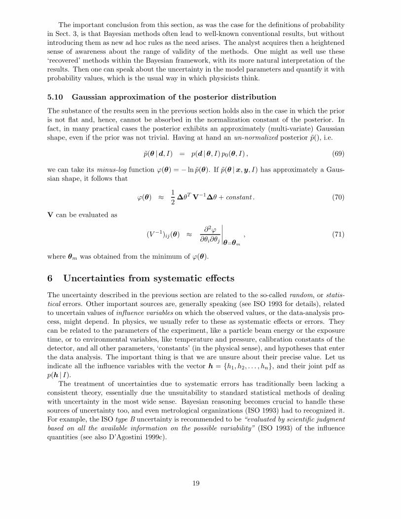
5.10 Gaussian approximation of the posterior distribution

The substance of the results seen in the previous section holds also in the case in which the prioris not flat and, hence, cannot be absorbed in the normalization constant of the posterior. Infact, in many practical cases the posterior exhibits an approximately (multi-variate) Gaussianshape, even if the prior was not trivial. Having at hand an un-normalized posterior p(), i.e.

p(θ |d, I) = p(d |θ, I) p0(θ, I) , (69)

we can take its minus-log function ϕ(θ) = − ln p(θ). If p(θ |x,y, I) has approximately a Gaus-sian shape, it follows that

ϕ(θ) ≈ 12

∆θT V−1∆θ + constant . (70)

V can be evaluated as

(V −1)ij(θ) ≈ ∂2ϕ

∂θi∂θj

∣∣∣∣∣θ=θm

, (71)

where θm was obtained from the minimum of ϕ(θ).

6 Uncertainties from systematic effects

The uncertainty described in the previous section are related to the so-called random, or statis-tical errors. Other important sources are, generally speaking (see ISO 1993 for details), relatedto uncertain values of influence variables on which the observed values, or the data-analysis pro-cess, might depend. In physics, we usually refer to these as systematic effects or errors. Theycan be related to the parameters of the experiment, like a particle beam energy or the exposuretime, or to environmental variables, like temperature and pressure, calibration constants of thedetector, and all other parameters, ‘constants’ (in the physical sense), and hypotheses that enterthe data analysis. The important thing is that we are unsure about their precise value. Let usindicate all the influence variables with the vector h = h1, h2, . . . , hn, and their joint pdf asp(h | I).

The treatment of uncertainties due to systematic errors has traditionally been lacking aconsistent theory, essentially due the unsuitability to standard statistical methods of dealingwith uncertainty in the most wide sense. Bayesian reasoning becomes crucial to handle thesesources of uncertainty too, and even metrological organizations (ISO 1993) had to recognized it.For example, the ISO type B uncertainty is recommended to be “evaluated by scientific judgmentbased on all the available information on the possible variability” (ISO 1993) of the influencequantities (see also D’Agostini 1999c).

19

6.1 Reweighting of conditional inferences

The values of the influence variables and their uncertainties contribute to our background knowl-edge I about the experimental measurements. Using I0 to represent our very general backgroundknowledge, the posterior pdf will then be p(µ |d,h, I0), where the dependence on all possiblevalues of h has been made explicit. The inference that takes into account the uncertain vectorh is obtained using the rules of probability (see Tab. 1) by integrating the joint probability overthe uninteresting influence variables:

p(µ |d, I0) =∫

p(µ,h |d, I0) dh (72)

=∫

p(µ |d,h, I0) p(h | I0) dh . (73)

As a simple, but important case, let us consider a single influence variable given by an additiveinstrumental offset z, which is expected to be zero because the instrument has been calibratedas well as feasible and the remaining uncertainty is σz. Modelling our uncertainty in z as aGaussian distribution with a standard deviation σz, the posterior for µ is

p(µ | d, I0) =∫ +∞

−∞p(µ | d, z, σ, I0) p(z |σz, I0) dz (74)

=∫ +∞

−∞1√2π σ

exp

[−(µ− (d− z))2

2σ2

]×

1√2π σz

exp

[− z2

2σ2z

]dz (75)

=1√

2π√

σ2 + σ2z

exp

[− (µ− d)2

2 (σ2 + σ2z)

]. (76)

The result is that the net variance is the sum of the variance in the measurement and thevariance in the influence variable.

6.2 Joint inference and marginalization of nuisance parameters

A different approach, which produces identical results, is to think of a joint inference about boththe quantities of interest and the influence variables:

p(µ,h |d, I0) ∝ p(d |µ,h, I0) p0(µ,h | I0) . (77)

Then, marginalization is applied to the variables that we are not interested in (the so callednuisance parameters), obtaining

p(µ|d, I0) =∫

p(µ,h |d, I0) dh (78)

∝∫

p(d |µ,h, I0) p0(µ,h | I0) dh . (79)

Equation (77) shows a peculiar feature of Bayesian inference, namely the possibility making aninference about a number of variables larger than the number of the observed data. Certainly,there is no magic in it, and the resulting variables will be highly correlated. Moreover, theprior cannot be improper in all variables. But, by using informative priors in which expertsfeel confident, this feature allows one to tackle complex problems with missing or corruptedparameters. In the end, making use of marginalization, one can concentrate on the quantitiesof real interest.

20

The formulation of the problem in terms of Eqs. (77) and (79) allows one to solve problems inwhich the influence variables might depend on the true value µ, because p0(µ,h | I0) can modeldependences between µ and h. In most applications, h does not depend on µ, and the priorfactors into the product of p0(µ | I0) and p0(h | I0). When this happens, we recover exactly thesame results as obtained using the reweighting of conditional inferences approach described justabove.

6.3 Correlation in results caused by systematic errors

We can easily extend Eqs. (73), (77), and (79) to a joint inference of several variables, which,as we have seen, are nothing but parameters θ of suitable models. Using the alternative waysdescribed in Sects. 6.1 and 6.2, we have

p(θ |d,h, I0) ∝ p(d |θ,h, I0) p0(θ | I0) (80)

p(θ |d, I0) =∫

p(θ |d,h, I0) p(h | I0) dh (81)

and

p(θ,h |d, I0) ∝ p(d |θ,h, I0) p0(θ,h | I0) (82)

p(θ|d, I0) =∫

p(θ,h |d, I0) dh , (83)

respectively. The two ways lead to an identical result, as it can be seen comparing Eqs. (81)and (83).

Take a simple case of a common offset error of an instrument used to measure various quan-tities µi, resulting in the measurements di. We model each measurement as µi plus an error thatis Gaussian distributed with a mean of zero and a standard deviation σi. The calculation of theposterior distribution can be performed analytically, with the following results (see D’Agostini1999c for details):

• The uncertainty in each µi is described by a Gaussian centered at di, with standarddeviation σ(µi) =

√σ2

i + σ2z , consistent with Eq. (76).

• The joint posterior distribution p(µ1, µ2, . . .) does not factorize into the product of p(µ1),p(µ2), etc., because correlations are automatically introduced by the formalism, consistentwith the intuitive thinking of what a common systematic should do. Therefore, the jointdistribution will be a multi-variate Gaussian that takes into account correlation terms.

• The correlation coefficient between any pair µi, µj is given by

ρ(µi, µj) =σ2

z

σ(µi)σ(µj)=

σ2z√

(σ2i + σ2

z) (σ2j + σ2

z). (84)

We see that ρ(µi, µj) has the behavior expected from a common offset error; it is non-negative; it varies from practically zero, indicating negligible correlation, when (σz σi),to unity (σz σi), when the offset error dominates.

6.4 Approximate methods and standard propagation applied to systematicerrors

When we have many uncertain influence factors and/or the model of uncertainty is non-Gaussian,the analytic solution of Eq. (73), or Eqs. (77)–(79) can be complicated, or not existing at all.

21

Then numeric or approximate methods are needed. The most powerful numerical methods arebased on Monte Carlo (MC) techniques (see Sect. 9 for a short account). This issue goes beyondthe aim of this report. In a recent comprehensive particle-physics paper by Ciuchini et al (2001),these ideas have been used to infer the fundamental parameters of the Standard Model of particlephysics, using all available experimental information.

For routine use, a practical approximate method can be developed by thinking of the valueinferred for the expected value of h as a raw value, indicated with µR, that is, µR = µ

∣∣∣h=E(h)

(‘raw’ in the sense that it needs later to be ‘corrected’ for all possible value of θ, as it will beclear in a while). The value of µ, which depends on the possible values of h, can be seen as afunction of µR and h:

µ = f(µR,h) . (85)

We have thus turned our inferential problem into a standard problem of evaluation of the pdf of afunction of variables, of which are particularly known the formulae to obtain approximate valuesfor expectations and standard deviations in the case of independent input quantities (followingthe nomenclature of ISO 1993):

E(µ) ≈ f(E(µR),E(h)) (86)

σ2(µ) ≈(

∂f

∂µR

∣∣∣∣E(µR),E(h)

)2

σ2(µR)

+∑

i

(∂f

∂hi

∣∣∣∣E(µR),E(h)

)2

σ2(hi) . (87)

Extension to multi-dimensional problems and treatment of correlations is straightforward (thewell-known covariance matrix propagation) and we refer to (D’Agostini and Raso 1999) fordetails. In particular, this reference contains approximate formulae valid up to second order,which allow to take into account relatively easily non linearities.

7 Comparison of models of different complexity

We have seen so far two typical inferential situations:

1. Comparison of simple models (Sect. 4), where by simple we mean that the models do notdepend on parameters to be tuned to the experimental data.

2. Parametric inference given a model, to which we have devoted the last sections.

A more complex situation arises when we have several models, each of which might depend onseveral parameters. For simplicity, let us consider model A with nA parameters α and model Bwith nB parameters β. In principle, the same Bayesian reasoning seen previously holds:

P (A |Data, I)P (B |Data, I)

=P (Data |A, I)P (Data |B, I)

P (A | I)P (B | I)

, (88)

but we have to remember that the probability of the data, given a model, depends on theprobability of the data, given a model and any particular set of parameters, weighted with theprior beliefs about parameters. We can use the same decomposition formula (see Tab. 1), alreadyapplied in treating systematic errors (Sect. 6):

P (Data |M, I) =∫

P (Data |M,θ, I) p(θ | I) dθ , (89)

22

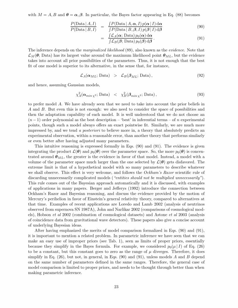
with M = A,B and θ = α,β. In particular, the Bayes factor appearing in Eq. (88) becomes

P (Data |A, I)P (Data |B, I)

=∫P (Data |A,α, I) p(α | I) dα∫P (Data |B,β, I) p(β | I) dβ

(90)

=∫LA(α; Data) p0(α) dα∫LB(β; Data) p0(β) dβ

. (91)

The inference depends on the marginalized likelihood (89), also known as the evidence. Note thatLM (θ; Data) has its largest value around the maximum likelihood point θML, but the evidencetakes into account all prior possibilities of the parameters. Thus, it is not enough that the bestfit of one model is superior to its alternative, in the sense that, for instance,

LA(αML; Data) > LB(βML; Data) , (92)

and hence, assuming Gaussian models,

χ2A(αmin χ2 ; Data) < χ2

B(βmin χ2 ; Data) , (93)

to prefer model A. We have already seen that we need to take into account the prior beliefs inA and B. But even this is not enough: we also need to consider the space of possibilities andthen the adaptation capability of each model. It is well understood that we do not choose an(n− 1) order polynomial as the best description – ‘best’ in inferential terms – of n experimentalpoints, though such a model always offers an exact pointwise fit. Similarly, we are much moreimpressed by, and we tend a posteriori to believe more in, a theory that absolutely predicts anexperimental observation, within a reasonable error, than another theory that performs similarlyor even better after having adjusted many parameters.

This intuitive reasoning is expressed formally in Eqs. (90) and (91). The evidence is givenintegrating the product L(θ) and p0(θ) over the parameter space. So, the more p0(θ) is concen-trated around θML, the greater is the evidence in favor of that model. Instead, a model with avolume of the parameter space much larger than the one selected by L(θ) gets disfavored. Theextreme limit is that of a hypothetical model with so many parameters to describe whateverwe shall observe. This effect is very welcome, and follows the Ockham’s Razor scientific rule ofdiscarding unnecessarily complicated models (“entities should not be multiplied unnecessarily”).This rule comes out of the Bayesian approach automatically and it is discussed, with examplesof applications in many papers. Berger and Jefferys (1992) introduce the connection betweenOckham’s Razor and Bayesian reasoning, and discuss the evidence provided by the motion ofMercury’s perihelion in favor of Einstein’s general relativity theory, compared to alternatives atthat time. Examples of recent applications are Loredo and Lamb 2002 (analysis of neutrinosobserved from supernova SN 1987A), John and Narlikar 2002 (comparisons of cosmological mod-els), Hobson et al 2002 (combination of cosmological datasets) and Astone et al 2003 (analysisof coincidence data from gravitational wave detectors). These papers also give a concise accountof underlying Bayesian ideas.

After having emphasized the merits of model comparison formalized in Eqs. (90) and (91),it is important to mention a related problem. In parametric inference we have seen that we canmake an easy use of improper priors (see Tab. 1), seen as limits of proper priors, essentiallybecause they simplify in the Bayes formula. For example, we considered p0(µ | I) of Eq. (26)to be a constant, but this constant goes to zero as the range of µ diverges. Therefore, it doessimplify in Eq. (26), but not, in general, in Eqs. (90) and (91), unless models A and B dependon the same number of parameters defined in the same ranges. Therefore, the general case ofmodel comparison is limited to proper priors, and needs to be thought through better than whenmaking parametric inference.

23

8 Choice of priors – a closer look

So far, we have considered mainly likelihood-dominated situations, in which the prior pdf canbe included in the normalization constant. But one should be careful about the possibilityof uncritically use uniform priors, as a ‘prescription,’ or as a rule, though the rule might beassociated with the name of famous persons. For instance, having made N interviews to inferthe proportion θ of a population that supports a party, it is not reasonable to assume a uniformprior of θ between 0 and 1. Similarly, having to infer the rate r of a Poisson process (suchthat λ = r T , where T is the measuring time) related, for example, to proton decay, cosmic rayevents or gravitational wave signals, we do not believe, strictly, that p(r) is uniform betweenzero and infinity. Besides natural physical cut-off’s (for example, very large proton decay rwould prevent Life, or even stars, to exist), p(r) = constant implies to believe more high ordersof magnitudes of r (see Astone and D’Agostini 1999 for details). In many cases (for example thementioned searches for rare phenomena) our uncertainty could mean indifference over severalorders of magnitude in the rate r. This indifference can be parametrized roughly with a prioruniform ln r yielding p(r) ∝ 1/r (the same prior is obtainable using invariant arguments, as itwill be shown in a while).

As the reader might imagine, the choice of priors is a highly debated issue, also amongBayesians. We do not pretend to give definitive statements, but would just like to touch onsome important issues concerning priors.

8.1 Logical and practical role of priors

Priors are pointed to by those critical of the Bayesian approach as the major weakness of thetheory. Instead, Bayesians consider them a crucial and powerful key point of the method.Priors are logically crucial because they are necessary to make probability inversions via Bayes’theorem. This point remains valid even in the case in which they are vague and apparentlydisappear in the Bayes’ formula. Priors are powerful because they allow to deal with realisticsituations in which informative prior knowledge can be taken into account and properly balancedwith the experimental information.

Indeed, we think that one of the advantages of Bayesian analysis is that it explicitly admitsthe existence of prior information, which naturally leads to the expectation that the prior willbe specified in any honest account of a Bayesian analysis. This crucial point is often obscured inother types of analyses, in large part because the analysts maintain their method is ‘objective.’Therefore, it is not easy, in those analyses, to recognize what are the specific assumptions madeby the analyst — in practice the analyst’s priors — and the assumptions included in the method(the latter assumptions are often unknown to the average practitioner).

8.2 Purely subjective assessment of prior probabilities

In principle, the point is simple, at least in one-dimensional problem in which there is goodperception of the possible range in which the uncertain variable of interest could lie: try yourbest to model your prior beliefs. In practice, this advice seems difficult to follow because, even ifwe have a rough idea of what the value of a quantity should be, the representation of the prior inmathematical terms seems very committal, because a pdf implicitly contains an infinite numberof precise probabilistic statements. (Even the uniform distribution says that we believe exactly inthe same way to all values. Who believes exactly that?) It is then important to understand that,when expressing priors, what matters is not the precise mathematical formula, but the grossvalue of the probability mass indicated by the formula, how probabilities are intuitively perceivedand how priors influence posteriors. When we say, intuitively, we believe something with a 95%confidence, it means “we are almost sure,” but the precise value (95%, instead of 92% or 98%)

24

is not very relevant. Similarly, when we say that the prior knowledge is modeled by a Gaussiandistribution centered around µ0 with standard deviation σ0 [Eq. (28)], it means means that weare quite confident that µ is within ±σ0, very sure that it is within ±2σ0 and almost certainthat it is within ±3σ0. Values even farther from µ0 are possible, though we do not considerthem very likely. But all models should be taken with a grain of salt, remembering that they areoften just mathematical conveniences. For example, a textbook-Gaussian prior includes infinitedeviations from the expected value and even negative values for physical quantities positivelydefined, like a temperature or a length. All absurdities, if taken literally. On the other hand, wethink that all experienced physicists have in mind priors with low probability long tails in orderto accommodate strong deviation from what is expected with highest probability. (Rememberthat where the prior is zero, the posterior must also be zero.)

Summing up this point, it is important to understand that a prior should tell where theprobability mass is concentrated, without taking too seriously the details, especially the tailsof the distribution (which should be, however, enough extended to accommodate ’surprises’).The nice feature of Bayes’ theorem is the ability of trasform such vague, fuzzy priors into solidestimates, if a sufficient amount of good quality data are at hand. For this reason, the useof improper priors is not considered to be problematic. Indeed, improper priors can just beconsidered a convenient way of modelling relative beliefs.

In the case we have doubts about the choice of the prior, we can consider a family of functionswith some hyperparameters. If we worry about the effect of the chosen prior on the posterior,we can perform a sensitivity analysis, i.e. to repeat the analysis for different, reasonable choicesof the prior and check the variation of the result. The final uncertainty could, then, take intoaccount also the uncertainty on the prior. Finally, in extreme cases in which priors play a crucialrole and could dramatically change the conclusions, one should refrain to give probabilistic result,providing, instead, only Bayes factors, or even just likelihoods. An example of a recent resultabout gravitational wave searches presented in this way, see Astone et al (2002).

Having clarified meaning and role of priors, it is rather evident that the practical choice of aprior depends on what is appropriate for the application. For example, in the area of imaging,smoothness of a reconstructed image might be appropriate in some situations. Smoothness maybe imposed by a variety of means, for example, by simply setting the logarithm of the priorequal to an integral of the square of the second derivative of the image (von der Linden et al1996b). A more sophisticated approach goes under the name of Markov random fields (MRF),which can even preserve sharp edges in the estimated images (Bouman and Sauer 1993, Saquibet al 1997). A similar kind of prior is often appropriate for defomable geometric models, whichcan be used to represent the boundaries between various regions, for example, organs in medicalimages (Cunningham et al 1998).

A procedure that helps in choosing the prior, expecially important in the cases in whichthe parameters do not have a straightforwardly perceptible influence on data, is to build aprior predictive pdf and check if this pdf would produce data conform with our prior beliefs.The prior predictive distribution is the analogue of the (posterior) predictive distribution wemet in Sect. 5.7, with p(θ |d, I) replaced by p(θ | I) (note that the example of Sect. 5.7 wasone-dimensional, with d1 = df and θ1 = µ), i.e. p(d | I) =

∫p(d |θ, I) p(θ | I) dθ.

Often, expecially in complicated data analyses, we are not sufficiently knowledgable aboutthe details of the problem. Thus, informative priors have to be modelled that capture thejudgement of experts. For example, Meyer and Booker (2001) show a formal process of priorelicitation which has the aim at reducing, as much as possible, the bias in the experts’ estimatesof their confidence limits. This approach allows one to combine the results from several experts.In short, we can suggest the use of the ‘coherent bet’ (Sect. 2) to force experts to access theirvalues of probability, asking them to provide an interval in which they feel ‘practically sure’,intervals on which they could wager 1:1, and so on.

25

8.3 Conjugate priors

Because of computational problems, modelling priors has been traditionally a compromise be-tween a realistic assessment of beliefs and choosing a mathematical function that simplifies theanalytic calculations. A well-known strategy is to choose a prior with a suitable form so theposterior belongs to the same functional family as the prior. The choice of the family depends onthe likelihood. A prior and posterior chosen in this way are said to be conjugate. For instance,given a Gaussian likelihood and choosing a Gaussian prior, the posterior is still Gaussian, as wehave seen in Eqs. (25), (28) and (29). This is because expressions of the form

K exp

[−(x1 − µ)2

2σ21

− (x2 − µ)2

2σ22

]

can always be written in the form

K ′ exp

[−(x′ − µ)2

2σ′2

],

with suitable values for x′, σ′ and K ′. The Gaussian distribution is auto-conjugate. Themathematics is simplified but, unfortunately, only one shape is possible.

An interesting case, both for flexibility and practical interest is offered by the binomiallikelihood (see Sect. 5.3). Apart from the binomial coefficient, p(n | θ,N) has the shape θn(1 −θ)N−n, which has the same structure as the Beta distribution, well known to statisticians:

Beta(θ | r, s) =1

β(r, s)θr−1(1− θ)s−1

0 ≤ θ ≤ 1r, s > 0

, (94)

where β(r, s) stands for the Beta function, defined as

β(r, s) =∫ 1

0θr−1(1− θ)s−1 dθ (95)

which can be expressed in terms of Euler’s Gamma function as β(r, s) = Γ(r) Γ(s)/Γ(r + s).Expectation and variance of the Beta distribution are:

E(θ) =r

r + s(96)

σ2(θ) =r s

(r + s + 1)(r + s)2= E2(θ)

s

r

1r + s + 1

. (97)

If r > 1 and s > 1, then the mode is unique, and it is at θm = (r − 1)/(r + s − 2). Dependingon the value of the parameters the Beta pdf can take a large variety of shapes. For example, forlarge values of r and s, the function is very similar to a Gaussian distribution, while a constantfunction is obtained for r = s = 1. Using the Beta pdf as prior function in inferential problemswith a binomial likelihood, we have

p(θ |n,N, r, s) ∝[θn(1− θ)N−n

] [θr−1(1− θ)s−1

](98)

∝ θn+r−1(1− θ)N−n+s−1 . (99)

The posterior distribution is still a Beta with r′ = r+n and s′ = s+N−n, and expectation andstandard deviation can be calculated easily from Eqs. (96) and (97). These formulae demonstratehow the posterior estimates become progressively independent of the prior information in thelimit of large numbers; this happens when both m r and n−m s. In this limit, we get thesame result as for a uniform prior (r = s = 1).

Table 2 lists some of the more useful conjugate priors. For a more complete collection of conjugatepriors, see e.g. (Bernardo and Smith 1994, Gelman et al 1995).

26

Table 2: Some useful conjugate priors. x and n stand for the observed value (continuous ordiscrete, respectively) and θ is the generic symbol for the parameter to infer, corresponding toµ of a Gaussian, θ of a binomial and λ of a Poisson distribution.

likelihood conjugate prior posteriorp(x | θ) p0(θ) p(θ |x)Normal(θ, σ) Normal(µ0, σ0) Normal(µ1, σ1) [Eqs. (30)–(32)]Binomial(N, θ) Beta(r, s) Beta(r + n, s + N − n)Poisson(θ) Gamma(r, s) Gamma(r + n, s + 1)Multinomial(θ1, . . . , θk) Dirichlet(α1, . . . , αk) Dirichlet(α1 + n1, . . . , αk + nk)

8.4 General principle based priors

Many who advocate using the Bayesian approach still want to keep ‘subjective’ contributions tothe inference to a minimum. Their aim is to derive prior functions based on ‘objective’ argumentsor general principles. As the reader might guess, this subject is rather controversial, and the riskof trasforming arguments, which might well be reasonable and useful in many circumstances,into dogmatic rules is high (D’Agostini, 1999e).

8.4.1 Transformation invariance

An important class of priors arises from the requirement of transformation invariance. We shallconsider two specific cases, translation invariance and scale invariance.

Translation invarianceLet us assume we are indifferent over a transformation of the kind θ′ = θ + b, where θ isour variable of interest and b a constant. Then p(θ) dθ is an infinitesimal mass element ofprobability for θ to be in the interval dθ. Translation invariance requires that this masselement remains unchanged when expressed in terms of θ′, i.e.

p(θ) dθ = p(θ′) dθ′ (100)= p(θ + b) dθ , (101)

since dθ = dθ′. It is easy to see that in order for Eq. (101) to hold for any b, p(θ) must beequal to a constant for all values of θ from −∞ to +∞. It is therefore an improper prior.As discussed above, this is just a convenient modelling. For practical purposes this priorshould always be regarded as the limit for ∆θ → ∞ of p(θ) = 1/∆θ, where ∆θ is a largefinite range around the values of interest.

Scale invarianceIn other cases, we could be indifferent about a scale transformation, that is θ′ = β θ, whereβ is a constant. This invariance implies, since dθ′ = β dθ in this case,

p(θ) dθ = p(β θ)β dθ , (102)

i.e.

p(β θ) =p(θ)β

. (103)

The solution of this functional equation is

p(θ) ∝ 1θ

, (104)

27

as can be easily proved using Eq. (104) as test solution in Eq. (103). This is the famousJeffreys’ prior, since it was first proposed by Jeffreys. Note that this prior also can bestated as p(log θ) = constant, as can be easily verified. The requirement of scale invariancealso produces an improper prior, in the range 0 < θ < ∞. Again, the improper prior mustbe understood as the limit of a proper prior extending several orders of magnitude aroundthe values of interest. [Note that we constrain θ to be positive because, traditionally,variables which are believed to satisfy this invariance are associated with positively definedquantities. Indeed, Eq. (104) has a symmetric solution for negative quantities.]

According to the supporters of these invariance motivated priors (see e.g. Jaynes 1968, 1973,1998, Sivia 1997, and Frohner 2000, Dose 2002) variables associated to translation invarianceare location parameters, as the parameter µ in a Gaussian model; variables associated to scaleinvariance are scale parameters, like σ in a Gaussian model or λ in a Poisson model. For criticismabout the (mis-)use of this kind of prior see (D’Agostini 1999d).

8.4.2 Maximum-entropy priors

Another principle-based approach to assigning priors is based on in the Maximum Entropyprinciple (Jaynes 1957a, also 1983, 1998, Tribus 1969, von der Linden 1995, Sivia 1997, andFrohner 2000). The basic idea is to choose the prior function that maximizes the Shannon-Jaynes information entropy,

S = −n∑i

pi ln pi , (105)

subject to whatever is assumed to be known about the distribution. The larger S is, thegreater is our ignorance about the uncertain value of interest. The value S = 0 is obtainedfor a distribution that concentrates all the probability into a single value. In the case of noconstraint other than normalization, (

∑ni pi = 1), S is maximized by the uniform distribution,

pi = 1/n, which is easily proved using Lagrange multipliers. For example, if the variable is aninteger between 0 and 10, a uniform distribution p(xi) = 1/11 gives S = 2.40. Any binomialdistribution with n = 10 gives a smaller value, with a maximum of S = 1.88 for θ = 1/2 and alimit of S = 0 for θ → 0 or or θ → 1, where θ is now the parameter of the binomial that givesthe probability of success at each trial.

Two famous cases of maximum-entropy priors for continuous variables are when the onlyinformation about the distribution is either the expected value or the expected value and thevariance. Indeed, these are special cases of general constraints on the moments of the distributionMr (see Tab. 1). For r = 0 and 1, Mr is equal to unity and to the expected value, respectively.First and second moment together provide the variance (see Tab. 1 and Sect. 5.6). Let us sumup what the assumed knowledge on the various moments provides [see e.g. (Sivia 1997, Dose2002)].

Knowledge about M0

Normalization alone provides a uniform distribution over the interval in which the variableis defined:

p(θ |M0 = 1) =1

b− aa ≤ θ ≤ b . (106)

This is the extension to continuous variables of the discrete case we saw above.

Knowledge about M0 and M1 [i.e. about E(θ)]Adding to the constraint M0 = 1 the knowledge about the expectation of the variable,

28

plus the requirement that all non-negative values are allowed, an exponential distributionis obtained:

p(θ |M0 = 1,M1 ≡ E(θ)) =1

E(θ)e−θ/E(θ) 0 ≤ θ < ∞ . (107)

Knowledge about M0, M1 and M2 [i.e. about E(θ) and σ(θ)]Finally, the further constraint provided by the standard deviation (related to first andsecond moment by the equation σ2 = M2 − M2

1 ) yields a prior with a Gaussian shapeindependently of the range of θ, i.e.

p(θ |M0 = 1,E(θ), σ(θ)) =exp

[− (θ−E(θ))2

2 σ2(θ)

]∫ ba exp

[− (θ−E(θ))2

2 σ2(θ)

]dθ

a ≤ θ ≤ b .

(108)

The standard Gaussian is recovered when θ is allowed to be any real number.

Note, however, that the counterpart of Eq. (105) for continuous variables is not trivial, since allpi of Eq. (105) tend to zero. Hence the analogous functional form

∫p(θ) ln p(θ) dθ no longer has

a sensible interpretation in terms of uncertainty, as remarked by Bernardo and Smith (1994).The Jaynes’ solution is to introduce a ‘reference’ density m(θ) to make entropy invariant undercoordinate transformation via

∫p(θ) ln[p(θ)/m(θ)] dθ. (It is important to remark that the first

and the third case discussed above are valid under the assumption of a unity reference density.)This solution is not universally accepted (see Bernardo and Smith 1994), even though it conformsto the requirements of dimensional analysis. Anyhow, besides formal aspects and the undeniableaid of Maximum Entropy methods in complicate problems such as image reconstruction (Buckand Macauly 1991), we find it very difficult, if not impossible at all, that a practitioner holds thatstatus of knowledge which give rise to the two celebrated cases discussed above. We find morereasonable the approach described in Sect. 8.2, that goes the other way around: we have a roughidea of where the quantity of interest could be, then we try to model it and to summarize it interms of expected value and standard deviation. In particular, we find untenable the position ofthose who state that Gaussian distribution can only be justified by Maximum Entropy principle.

8.4.3 Reference priors

We conclude this discussion on priors by mentioning ‘reference analysis,’ which is an area ofactive research among statisticians. The intention is, similarly to that for other priors motivatedby basic principles, that of “characterizing a ‘non-informative’ or ‘objective’ prior distribution,representing ‘prior ignorance,’ ‘vague prior knowledge,’ and ‘letting the data speak for themselves’” (Bernardo and Smith 1994). However, “the problem is more complex than the apparentintuitive immediacy of these words and phrases would suggest” (Bernardo and Smith 1994,p. 298):

“Put bluntly: data cannot ever speak entirely for themselves: every prior specification hassome informative posterior or predictive implications; and ‘vague’ is itself much too vaguean idea to be useful. There is no ‘objective’ prior that represents ignorance.

On the other hand, we recognize that there is often a pragmatically important need fora form of prior to posterior analysis capturing, in some well-defined sense, the notion of theprior having a minimal effect, relative to the data, on the final inference. Such a referenceanalysis might be required as an approximation to actual beliefs; more typically, it might berequired as a limiting ‘what if?’ baseline in considering a range of prior to posterior analyses,or as a default option when there are insufficient resources for detailed elicitation of actualprior knowledge.

29

. . . From the approach we adopt, it will be clear that the reference prior component of

the analysis is simply a mathematical tool. It has considerable pragmatic importance in

implementing a reference analysis, whose role and character will be precisely defined, but it

is not a privileged, ‘unique non-informative’ or ‘objective’ prior.”

The curious reader may take a look at the (Bernardo and Smith 1994) and references citedtherein, as well as at Bernardo (1997).

9 Computational issues

The application of Bayesian ideas leads to computational problems, mostly related to the cal-culation of integrals for normalizing the posterior pdf and for obtaining credibility regions, orsimply the moments of the distribution (and, hence, expectations, variances and covariances).The difficulties become challenging for problems involving many parameters. This is one of thereasons why Bayesian inference was abandoned at the beginning of the 20th century in favorof simplified – and simplistic – methods. Indeed, the Bayesian renaissance over the past fewdecades is largely due to the emergence of new numerical methods and the dramatic increasesin computational power, along with clarifying work on the foundations of the theory.

9.1 Overview of approximate computational strategies

In previous sections we have already seen some ‘tricks’ for simplifying the calculations. Themain topic of this section will be an introduction to Monte Carlo (MC). But, before doing that,we think it is important to summarize the various ‘tricks’ here. Much specialized literature isavailable on several aspects of computation in statistics. For an excellent review paper on thesubject see (Smith 1991).

Conjugate priorsWe discussed this topic in Sect. 8.3, giving a couple of typical simple examples and refer-ences for a more detailed list of famous conjugate distributions. We want to remark herethat a conjugate prior is a special case of the class of priors that simplify the calculationof the posterior (the uniform prior is the simplest of this kind of prior).

Gaussian approximationFor reasons that are connected with the central limit theorem, when there is a large amountof consistent data the posterior tends to be Gaussian, practically independently of the exactshape of the prior. The (multi-variate) Gaussian approximation, which we encountered inSect. 5.10, has an important role for applications, either as a reasonable approximationof the ‘true’ posterior, or as a starting point for searching for a more accurate descriptionof it. We also saw that in the case of practically flat priors this method recovers thewell-known minimum chi-square or maximum likelihood methods.

Numerical integrationIn the case of low dimensional problems, standard numerical integration using either scien-tific library functions or the interactive tools of modern computer packages provide an easysolution to many problems (thanks also to the graphical capabilities of modern programswhich allow the shape of the posterior to be inspected and the best calculation strategydecided upon). This is a vast and growing subject, into we cannot enter in any depth here,but we assume the reader is familiar with some of these programs or packages.

Monte Carlo methodsMonte Carlo methodology is a science in itself and it is way beyond our remit to provide

30

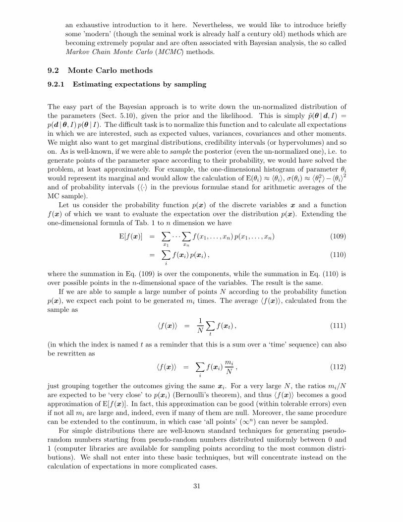
an exhaustive introduction to it here. Nevertheless, we would like to introduce brieflysome ’modern’ (though the seminal work is already half a century old) methods which arebecoming extremely popular and are often associated with Bayesian analysis, the so calledMarkov Chain Monte Carlo (MCMC) methods.

9.2 Monte Carlo methods

9.2.1 Estimating expectations by sampling

The easy part of the Bayesian approach is to write down the un-normalized distribution ofthe parameters (Sect. 5.10), given the prior and the likelihood. This is simply p(θ |d, I) =p(d |θ, I) p(θ | I). The difficult task is to normalize this function and to calculate all expectationsin which we are interested, such as expected values, variances, covariances and other moments.We might also want to get marginal distributions, credibility intervals (or hypervolumes) and soon. As is well-known, if we were able to sample the posterior (even the un-normalized one), i.e. togenerate points of the parameter space according to their probability, we would have solved theproblem, at least approximately. For example, the one-dimensional histogram of parameter θi

would represent its marginal and would allow the calculation of E(θi) ≈ 〈θi〉, σ(θi) ≈⟨θ2i

⟩−〈θi〉2and of probability intervals (〈·〉 in the previous formulae stand for arithmetic averages of theMC sample).

Let us consider the probability function p(x) of the discrete variables x and a functionf(x) of which we want to evaluate the expectation over the distribution p(x). Extending theone-dimensional formula of Tab. 1 to n dimension we have

E[f(x)] =∑x1

· · ·∑xn

f(x1, . . . , xn) p(x1, . . . , xn) (109)

=∑

i

f(xi) p(xi) , (110)

where the summation in Eq. (109) is over the components, while the summation in Eq. (110) isover possible points in the n-dimensional space of the variables. The result is the same.

If we are able to sample a large number of points N according to the probability functionp(x), we expect each point to be generated mi times. The average 〈f(x)〉, calculated from thesample as

〈f(x)〉 =1N

∑t

f(xt) , (111)

(in which the index is named t as a reminder that this is a sum over a ‘time’ sequence) can alsobe rewritten as

〈f(x)〉 =∑

i

f(xi)mi

N, (112)

just grouping together the outcomes giving the same xi. For a very large N , the ratios mi/Nare expected to be ‘very close’ to p(xi) (Bernoulli’s theorem), and thus 〈f(x)〉 becomes a goodapproximation of E[f(x)]. In fact, this approximation can be good (within tolerable errors) evenif not all mi are large and, indeed, even if many of them are null. Moreover, the same procedurecan be extended to the continuum, in which case ‘all points’ (∞n) can never be sampled.

For simple distributions there are well-known standard techniques for generating pseudo-random numbers starting from pseudo-random numbers distributed uniformly between 0 and1 (computer libraries are available for sampling points according to the most common distri-butions). We shall not enter into these basic techniques, but will concentrate instead on thecalculation of expectations in more complicated cases.

31

9.2.2 Rejection sampling

Let us assume we are able to generate points according to some function g(x), such that, givena constant c, p(x) ≤ cg(x). We generate x∗ according to g(x) and decide to accept it withprobability p(x∗)/cg(x∗) (i.e. we extract another random number between 0 and 1 and acceptthe point if this number is below that ratio). It is easy to show that this procedure reshapes g(x)to p(x) and that it does not depend on the absolute normalization of p(x) (any normalizationconstant can be absorbed in the multiplicative constant c). A trivial choice of g(x), especiallyfor simple one-dimensional problems, is a uniform distribution (this variation is known as thehit or miss method), though clearly it can be very inefficient.

9.2.3 Importance sampling

In this method, too, we start from an ‘easy’ function g(x), which ‘we hope’ will approximatep(x) of interest, of which in fact we know only its un-normalized expression p(x). However,there is no requirement about how g(x) approximates p(x) (but the goodness of approximationwill have an impact on the efficacy of the method), apart from the condition that g(xi) must bepositive wherever p(xi) is positive .

The function g(x) can be used in the calculation of E[f(x)], if we notice that E[f(x)] canbe rewritten as follows:

E[f(x)] =∫f(x) p(x) dx∫

p(x) dx(113)

=∫f(x) [p(x)/g(x)] g(x) dx∫

[p(x)/g(x)] g(x) dx(114)

=Eg [f(x) p(x)/g(x)]

Eg [p(x)/g(x)], (115)

where the the symbol Eg is a reminder that the expectation is calculated over the distributiong(x). Finally, the strategy can be implemented in the Monte Carlo using Eq. (111) for the twoexpectations:

E[f(x)] ≈∑

t f(xt) p(xt)/g(xt)∑t p(xt)/g(xt)

. (116)

From the same sample it is also possible to evaluate the normalization constant, given by thedenominator of Eq. (113), i.e.

Z =∫

p(x) dx ≈ 1N

∑t

p(xt)g(xt)

. (117)

The computation of this quantity is particularly important when we are dealing with modelcomparison and Z has the meaning of ‘evidence’ (Sect. 7).

It easily to see that the method works well if g(x) overlaps well with p(x). Thus, a properchoice of g(x) can be made by studying where the probability mass of p(x) is concentrated (forexample finding the mode of the distribution in a numerical way). Often a Gaussian functionis used for g(x), with parameters chosen to approximate p(x) in the proximity of the mode, asdescribed in Sect. 5.10. In other cases, other functions can be used which have more pronouncedtails, like t-Student or Cauchy distributions. Special techniques, into which we cannot enter here,allow n independent random numbers to be generated and, subsequently, by proper rotations,

32

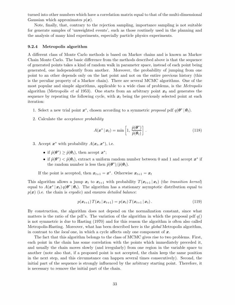
turned into other numbers which have a correlation matrix equal to that of the multi-dimensionalGaussian which approximates p(x).

Note, finally, that, contrary to the rejection sampling, importance sampling is not suitablefor generate samples of ‘unweighted events’, such as those routinely used in the planning andthe analysis of many kind experiments, especially particle physics experiments.

9.2.4 Metropolis algorithm

A different class of Monte Carlo methods is based on Markov chains and is known as MarkovChain Monte Carlo. The basic difference from the methods described above is that the sequenceof generated points takes a kind of random walk in parameter space, instead of each point beinggenerated, one independently from another. Moreover, the probability of jumping from onepoint to an other depends only on the last point and not on the entire previous history (thisis the peculiar property of a Markov chain). There are several MCMC algorithms. One of themost popular and simple algorithms, applicable to a wide class of problems, is the Metropolisalgorithm (Metropolis et al 1953). One starts from an arbitrary point x0 and generates thesequence by repeating the following cycle, with xt being the previously selected point at eachiteration:

1. Select a new trial point x∗, chosen according to a symmetric proposal pdf q(θ∗ |θt).

2. Calculate the acceptance probability

A(x∗ |xt) = min[1,

p(θ∗)p(θt)

]. (118)

3. Accept x∗ with probability A(xt,x∗), i.e.

• if p(θ∗) ≥ p(θt), then accept x∗;

• if p(θ∗) < p(θt), extract a uniform random number between 0 and 1 and accept x∗ ifthe random number is less then p(θ∗)/p(θt).

If the point is accepted, then xt+1 = x∗. Otherwise xt+1 = xt

This algorithm allows a jump xt to xt+1 with probability T (xt+1 |xt) (the transition kernel)equal to A(x∗ |xt) q(θ∗ |θt). The algorithm has a stationary asymptotic distribution equal top(x) (i.e. the chain is ergodic) and ensures detailed balance:

p(xt+1)T (xt |xt+1) = p(xt)T (xt+1 |xt) . (119)

By construction, the algorithm does not depend on the normalization constant, since whatmatters is the ratio of the pdf’s. The variation of the algorithm in which the proposal pdf q()is not symmetric is due to Hasting (1970) and for this reason the algorithm is often also calledMetropolis-Hasting. Moreover, what has been described here is the global Metropolis algorithm,in contrast to the local one, in which a cycle affects only one component of x.

The fact that this algorithm belongs to the class of MCMC gives rise to two problems. First,each point in the chain has some correlation with the points which immediately preceded it,and usually the chain moves slowly (and irregularly) from one region in the variable space toanother (note also that, if a proposed point is not accepted, the chain keep the same positionin the next step, and this circumstance can happen several times consecutively). Second, theinitial part of the sequence is strongly influenced by the arbitrary starting point. Therefore, itis necessary to remove the initial part of the chain.

33

Using an MCMC for a complex problem is not an automatic procedure and some tuning isneeded. One of the important things to choose with care is the proposal function. If too smalljumps are proposed, the chain moves too slowly and, can even remain trapped in a subregionand never sample the rest of the parameter space, if the probability distribution is defined overdisconnected regions. If too large steps are proposed, the proposed points could often fall invery low probability regions and not be accepted, in which case the chain remains stuck in apoint for many cycles.

For an interesting, insightful introduction to principles and applications of MCMC see (Kasset al 1998). A nice tutorial is given by (Hanson 2000). A recent application of Bayesianmethods in cosmology, which uses MCMC and contains a pedagogical introduction too, canbe found in (Lewis and Bridle 2002). For a good treatise, freely available on the web, (Neel1993) is recommended. The reader will find that MCMC techniques are used to solve complexproblems graphically represented in terms of Bayesian networks (also known as belief networksor simply probabilistic network). This subject, which has revolutionized the way of thinkingartificial intelligence and the uncertainty issues related to it, does beyond the purpose of thisarticle. The interested reader can find more information in (Pearl 1988, BUGS 1996, Cowell etal 1999 and Cozman 2001) and references therein.

10 Conclusions

The gain in popularity Bayesian methods have enjoyed in recent years is due to various concep-tual and practical advantages they have over other approaches, among which are:

• the recovery of the intuitive idea of probability as a valid concept for treating scientificproblems;

• the simplicity and naturalness of the basic tool;

• the capability of combining prior knowledge and experimental information;

• the property permitting automatic updating as soon as new information becomes available;

• the transparency of the methods, which allow the different assumptions upon which aninference may depend to be checked and changed;

• the high degree of awareness the methods give to the user.

In this article we have seen how to build a theory of uncertainty in measurement as a straight-forward application of the basic Bayesian ideas, without unnecessary principles or ad hoc pre-scriptions. In particular, the uncertainty due to systematic errors can be treated in a consistentand powerful way.

Providing an exact solution for inferential problems can easily lead to computational dif-ficulties. We have seen several ways to overcome such difficulties, either by using suitableapproximations, or by using modern computational methods. In particular, it has been shownthat the approximate solution often coincides with a ‘conventional’ method, but only under welldefined conditions. Thus, for example, minimum χ2 formulae can be used, with a Bayesian spiritand with a natural interpretation of the results, in all those routine cases in which the analystconsiders as reasonable the conditions of their validity.

A variety of examples of applications have been shown, or mentioned, in this paper.Nevertheless, the aim of the author was not to provide a complete review of Bayesian methodsand applications, but rather to introduce those Bayesian ideas that could be of help inunderstanding more specialized literature. Compendia of the Bayesian theory are given in

34

(Bernardo and Smith 1994, O’Hagan A 1994 and Robert 2001). Classic, influential books are(Jeffreys 1961, de Finetti 1974, Jaynes 1998). Among the many books introducing Bayesianmethods, (Sivia 1996) is particularly suitable for physicists. Other recommended texts whichtreat general aspects of data analysis are (Box and Tiao 1973, Bretthorst 1988, Lee 1989,Gelman et al 1995, Cowell et al 1999, Denison et al 2002, Press 2002). More specific applicationscan be found in the proceedings of the conference series and several web sites. Some usefulstarting points for web navigation are given:

ISBA book list http://www.bayesian.org/books/books.htmlUAI proceedings http://www2.sis.pitt.edu/ dsl/UAI/uai.htmlBIPS http://astrosun.tn.cornell.edu/staff/loredo/bayes/BLIP http://www.ar-tiste.com/blip.htmlIPP Bayesian analysis group http://www.ipp.mpg.de/OP/Datenanalyse/Valencia meetings http://www.uv.es/∼bernardo/valenciam.htmlMaximum Entropy resources http://omega.albany.edu:8008/maxent.htmlMCMC preprint service http://www.statslab.cam.ac.uk/∼mcmc/

I am indebted to Volker Dose and Ken Hanson for extensive discussions concerning the contentsof this paper, as well as for substantial editorial help. The manuscript has also benefited fromcomments by Tom Loredo.

35

References

Astone P et al 2002 Search for correlation between GRB’s detected by BeppoSAX andgravitational wave detectors EXPLORER and NAUTILUS Phys. Rev. 66 102002.

Astone P and D’Agostini G 1999 Inferring the intensity of Poisson processes at limit ofdetector sensitivity (with a case study on gravitational wave burst search) CERN-EP/99-126

Astone P, D’Agostini G and D’Antonio 2003 Bayesian model comparison applied to theExplorer-Nautilus 2001 coincidence data, arXiv:gr-qc/0304096

Babu G J and Feigelson E D 1992 eds Statistical Challenges in Modern Astronomy I (NewYork: Springer)

Babu G J and Feigelson E D 1997 eds Statistical Challenges in Modern Astronomy II (NewYork: Springer)

Berger J O and Jefferys W H 1992 Sharpening Ockham’s razor on a Bayesian strop Am.Scientist 89 64–72 and J. Ital. Stat. Soc. 1 17

Bernardo J M 1999 ed Bayesian Methods in the Sciences, special issue of Rev. Acad. Cien.Madrid, 93(3)

Bernardo J M, J O Berger, A P Dawid and A F M Smith 1999 eds Bayesian Statistics 6(Oxford: Oxford University)

Bernardo J M and Smith F M 1994 Bayesian Theory (Chichester: John Wiley & Sons)

Bernardo J M 1997 Non-informative priors do not exist J. Stat. Planning and Infer. 65159

Bontekoe T R, Koper E and Kester D J M 1994 Pyramid maximum entropy images ofIRAS survey data Astron. Astrophys. 284 1037

Bouman C A and Sauer K 1993 A generalized Gaussian image model for edge-preservingMAP estimation IEEE Trans. on Image Processing 2 296

Box G E P and Tiao G C 1973 Bayesian inference in statistical analysis (Chichester: J.Wiley & Sons)

Bretthorst G L 1988 Bayesian spectrum analysis and parameter estimation (Berlin:Springer)

BUGS 1996 http://www.mrc-bsu.cam.ac.uk/bugs/welcome.shtml

Buck B and Macauly V A eds 1991 Maximum Entropy in action, (Oxford: Oxford Uni-versity Press)

Ciuchini M et al 2001 2000 CKM-Triangle Analysis: A critical review with updated ex-perimental inputs and theoretical parameters J. High Energy Phys. 0107 013

Coletti G and Scozzafava R 2002 Probabilistic logic in a coherent setting”, (Dordrecht:Kluwer Academic)

Cousins R D 1995 Why isn’t every physicist a Bayesian? Am. J. Phys. 63 398

36

Cowell R G, Dawid A P, Lauritzen S L and Spiegelhalter D J 1999 Probabilistic Networksand Expert Systems, (New York: Springer)

Cox R T 1946 Probability, Frequency and Reasonable Expectation Am. J. Phys. 14 1

Cozman F B 2001 JavaBayes version 0.346 – Bayesian networks in Java http://www-2.cs.cmu.edu/∼javabayes/Home/

Cunningham G S, Hanson K M and Battle X L 1998 Three-dimensional reconstructionsfrom low-count SPECT data using deformable models Opt. Expr. 2 227

D’Agostini G 1999a Bayesian Reasoning versus Conventional Statistics in High EnergyPhysics Maximum Entropy and Bayesian Methods ed von der Linden W et al (Dordrecht:Kluwer Academic)

D’Agostini G 1999b Sceptical combination of experimental results: General considerationsand application to epsilon-prime/epsilon CERN-EP/99-139

D’Agostini G 1999c Bayesian reasoning in high-energy physics: principles and applicationsCERN Report 99-03 (an extended version of this report is going to be published as Bayesianreasoning in data analysis – A critical introduction by World Scientific Publishing)

D’Agostini G 1999d Teaching statistics in the physics curriculum: Unifying and clarifyingrole of subjective probability Am. J. Phys. 67 1260

D’Agostini G 1999e Overcoming prior Anxiety, Bayesian Methods in the Sciences ed J. M.Bernardo; special issue of Rev. Acad. Cien. Madrid 93(3), 311

D’Agostini G 2000 Confidence limits: what is the problem? Is there the solution? CERNReport 2000-005 ed James F and Lyons L (Geneva: CERN) 3

D’Agostini G 2002 Minimum bias legacy of search results 2002 Nucl Phys Proc Suppl 109148

D’Agostini G and Degrassi G 1999 Constraints on the Higgs Boson Mass from DirectSearches and Precision Measurements Eur. Phys. J. C10 663

D’Agostini G and Raso M Uncertainties due to imperfect knowledge of systematic effects:general considerations and approximate formulae CERN-EP/2000-026

de Finetti B 1974 Theory of Probability (Chichester: J. Wiley & Sons)

Denison D G T, Holmes C C, Mallick B K and Smith A F M 2002 Bayesian methods fornonlinear classification and regression (Cichester: J. Wiley & Sons)

DIN (Deutsches Institut fur Normung) 1996 Grundlagen der Messtechnik - Teil 3: Auswer-tung von Messungen einer einzelnen Messgre, Messunsicherheit DIN 1319-3 (Berlin: BeuthVerlag)

DIN (Deutsches Institut fur Normung) 1999 Grundlagen der Messtechnik - Teil 4: Auswer-tung von Messungen, Messunsicherheit DIN 1319-4 (Berlin: Beuth Verlag)

Dose V 2002 Bayes in five days, CIPS, MPI fur Plasmaphysik, Garching, Germany, Reprint83, May 2002

37

Dose V and von der Linden W 1999 Outlier tolerant parameter estimation MaximumEntropy and Bayesian Methods ed von der Linden W et al (Dordrecht: Kluwer Academic)47

Efron B 1986a Why isn’t everyone a Bayesian? Am. Stat. 40 1

Efron B 1986b reply to Zellner 1986 Am. Stat. 40 331

Fischer R, Mayer M, von der Linden W and Dose V 1997 Enhancement of the energyresolution in ion-beam experiments with the maximum-entropy method Phys. Rev. E 556667

Fischer R, Mayer M, von der Linden W and Dose V 1998 Energy resolution enhancementin ion beam experiments with Bayesian probability theory Nucl. Instr. Meth. 136-1381140

Fischer R, Hanson K M, Dose V and von der Linden W 2000 Background estimation inexperimental spectra Phys. Rev. E61 1152

Frohner F H 2000 Evaluation and Analysis of Nuclear Resonance Data JEFF Report 18(Paris: OECD Publications)

Gelman A, Carlin J B, Stern H S and Rubin D B 1995 Bayesian Data Analysis (London:Chapman and Hall)

Glimm J and Sharp D H 1999 Prediction and the quantification of uncertainty Physica D133 152

Gregory P C and Loredo T J 1992 A new method for the detection of a periodic signal ofunknown shape and period Astr. J. 398 146

Gregory P C and Loredo T J 1996 Bayesian periodic signal detection II – Bayesian periodicsignal detection: analysis of ROSAT observations of PSR 0540-693 Astr. J. 473 1059

Gregory P C 1999 Bayesian periodic signal detection I – analysis of 20 years of radio fluxmeasurements of the x-ray binary LS I +61303 Astr. J. 520 361

Gubernatis J E, Jarrell M, Silver R N and Sivia D S 1991 Quantum Monte-Carlo sim-ulations and maximum-entropy: dynamics from imaginary-time data Phys. Rev. B 446011

Hanson K M 1993 Introduction to Bayesian image analysis Medical Imaging: Image Pro-cessing Loew M H ed Proc. SPIE 1898 716

Hanson K M 2000 Tutorial on Markov Chain Monte Carlo, http://public.lanl.gov/kmh/talks/maxent00b.pdf

Hasting W K 1970 Monte Carlo sampling methods using Markov chains and their appli-cations Biometrica 57 97

Higdon D M and Yamamoto S Y 2001 Estimation of the head sensitivity function inscanning magnetoresistance microscopy J. Amer. Stat. Assoc. 96 785

Hobson M P, Bridle S L and Lahav 2002 Combining cosmological datasets: hyperparam-eters and Bayesian evidence arXiv:astro-ph/0203259

38

Howson C and Urbach P 1993 Scientific reasoning — the Bayesian approach (Chicago andLa Salle: Open Court)

ISO (International Organization for Standardization) 1993 Guide to the Expression ofUncertainty in Measurement (Geneva: ISO)

Jaynes E T 1957a Information theory and statistical mechanics Phys. Rev. 106 620

Jaynes E T 1957b Information theory and statistical mechanics II Phys. Rev. 108 171

Jaynes E T 1968 Prior probabilities IEEE Trans. Syst. Cybern. SSC-4 227, reprinted in(Jaynes 1983)

Jaynes E T 1973 The well-posed problem Found. Phys. 3 477, reprinted in (Jaynes 1983)

Jaynes E T 1983 Papers on Probability, Statistics and Statistical Physics ed Harper W Land Hooker C A (Dordrecht: Reidel)

Jaynes E T 1998 http://omega.albany.edu:8008/JaynesBook.html

Jeffreys H 1961 Theory of Probability (Oxford: Oxford University)

John M V and Narlikar J V 2002 Comparison of cosmological models using Bayesian theoryPhys. Rev. D65 43506

Kadane J B and Schum D A 1996 A Probabilistic Analysis of the Sacco and VanzettiEvidence (Chichester: Wiley and Sons)

Kalman R E 1960 A new approach to linear filtering and prediction problems Trans.ASME Journal of Casic Engineering 82 35

Kass R E, Carlin B P, Gelman A and Neal R M 1998 Markov Chain Monte Carlo inpractice: A roundtable discussion Am. Stat. 52 93

Lad F 1996 Operational Subjective Statistical Methods – a Mathematical, Philosophical,and Historical Introduction (Chichester:J. Wiley & Sons)

Lee P M 1989 Bayesian statistics - an introduction (Chichester:J. Wiley & Sons)

Lewis A and Bridle S 2002 Cosmological parameters from CMB and other data: a Monte-Carlo approach Phys.Rev. D66 103511

von der Linden W 1995 Maximum-entropy data analysis Appl. Phys. A60 155

von der Linden W, Dose V and Fischer R 1996b Spline-based adaptive resolution imagereconstruction Proceedings of the 1996 Maximum Entropy Conference ed Sears M et al(Port Elizabeth: N.M.B. Printers) 154

Lindley D V 1986 Discussion to Efron 1986a Am. Stat. 40 6

Loredo T J 1990 Maximum Entropy and Bayesian Methods ed Fougere P F (Dordrecht:Kluwer Academic) 81

Loredo T J and Lamb D Q 2002 Bayesian analysis of neutrinos observed from supernovaSN 1987A Phys. Rev. D65 063002

Malakoff D 1999 Bayes Offers a ’New’ Way to Make Sense of Numbers Science 286 1460

39

Maybaeck P S 1979 Stochastic models, estimation and control, Vol. 1 (New York: AcademicPress).

Metropolis H, Rosenbluth A W, Rosenbluth M N, Teller A H and Teller E 1953 Equationsof state calculations by fast computing machines Journal of Chemical Physics 21 1087

von Mises R 1957 Probability, Statistics, and Truth (St Leonards: Allen and Unwin);reprinted in 1987 by Dover

Neal R M 1993 Probabilistic inference using Markov chain Monte Carlo methods (Toronto:Technical Report CRG-TR-93-1)

O’Hagan A 1994 Kendall’s Advanced Theory of Statistics: Vol. 2B - Bayesian Inference(New York: Halsted)

Pearl J 1988 Probabilistic Reasoning in Intelligent Systems: Networks of Plausible Inference(San Mateo: Morgan Kaufmann)

Press W H 1997 Understanding data better with Bayesian and global statistical methodsUnsolved problems in astrophysics49–60 ed Bahcall J N and Ostriker J P (Princeton:Princeton University) 49

Press S J 2002 Subjective and Objective Bayesian Statistics: Principles, Models, and Ap-plications 2nd Edition (Chichester: John Wiley & Sons)

Robert C P 2001 The Bayesian Choice (New York: Springer)

Saquib S S, Hanson K M, and Cunningham G S 1997 Model-based image reconstructionfrom time-resolved diffusion data Proc. SPIE 3034 369

Schrodinger E 1947a The Foundation of the Theory of Probability – I Proc. R. Irish Acad.51A 51; reprinted in Collected papers Vol. 1 (Vienna 1984: Austrian Academy of Science)463

Schrodinger E 1947b The Foundation of the Theory of Probability – II Proc. R. IrishAcad. 51A 141; reprinted in Collected papers Vol. 1 (Vienna 1984: Austrian Academy ofScience) 479

Sivia D S 1997 Data Analysis – a Bayesian Tutorial (Oxford: Clarendon)

Skilling J 1992 Quantified maximum entropy Int. Spectr. Lab. 2 4

Smith A F M 1991 Bayesian numerical analysis Phyl. Trans. R. Soc. London 337 369

Taylor B N and Kuyatt C E 1994 Guidelines for Evaluating and Expressing Uncertainty ofNIST Measurement Results (Gaithersburg: NIST Technical Note 1297); available on lineat http://physics.nist.gov/

Tribus M 1969 Rational Descriptions, Decisions, and Designs (Elmsford: Pergamon)

Welch G and Bishop G 2002 An introduction to Kalman filter (http://www.cs.unc.edu/∼welch/kalman/)

Zech G 2002 Frequentist and Bayesian confidence limits Eur. Phys. J. direct C12 1

Zellner A 1986 Bayesian solution to a problem posed by Efron Am. Stat. 40 330

40