Bayesian Inference - (An essential introduction)
35
Bayesian Inference (An essential introduction) L. Egidi Fall 2021 University of Trieste 1
Transcript of Bayesian Inference - (An essential introduction)

Bayesian Inference(An essential introduction)
L. EgidiFall 2021
University of Trieste
1

Basic ideas
Introducing Bayesian inference
2

Basic ideas

Bayes Theorem (basic)
• Bayes’ theorem is a rule to compute conditional probabilities.• In other words, it links probability measures on different spaces of
events: given two events E and H, the probability of H conditionalon E is the probability given to H knowing that E is true (i.e. E isthe new sample space (Ω)).
• More precisely,• I have given a probability measure on E and H,• I am told that E has occurred,• how do I change (if I change) my opinion on H:
P(H) → P(H|E) =?
Theorem of Bayes (for events) Let E and H be two events, assumeP(E ) 6= 0, then
P(H|E ) = P(H ∩ E )P(E ) = P(H)P(E |H)
P(E )
3

Bayes Theorem (an example: a crime case)
In an island a murder is committed
• there is no clue on who is the murderer;• but for the DNA found on the victim (who had a fight with the
murderer);• within the population of the island 1000 persons may have committed
the crime, it is a certain thing that the murderer is among them, withequal probability.
The police compares the DNA of all the 1000 suspects with that of themurderer.
The DNA test used by the island police force is not perfect, there is
• probability of a false positive 1%;• probability of a false negative 2%.
4

Bayes Theorem (an example: a crime case)
Formally, if
• T is the ‘event “the person is positive at the test”,• C is the event “the person is guilty”,
the two assumptions are then
• probability of a false positive 1% : P(T |C) = 0.01,• probability of a false negative 2% : P(T |C) = 0.02.
The experimental observation is: the police starts testing the 1000suspects and the 130-th is positive at testing.
5

Crime case: the investigation (likelihood inference)
The sheriff says that the experimental evidence, represented by the ratiobetween the likelihoods
P(T |C)P(T |C)
= 0.980.01 = 98
is overwhelmingly in favour of that person being guilty, thus constitutingdecisive evidence, so he asks the judge to arrest and condemn the guy.
Being more formal, who are model and likelihood?
• model: set of probability distributions which may have generated thesample T , there are two alternatives, represented by C , C:
P(T |C) = 0.98 P(T |C) = 0.01
• likelihood the parameter space is C , C, the likelihood takes twovalues
LC = P(T |C) = 0.98 LC = P(T |C) = 0.01• the maximum likelihood estimate is then C .
6

Crime case: the investigation (likelihood inference)
Even more formally,
• parameter: θ is 1 if the man is guilty, 0 otherwise (the parameterspace is then Θ = 0, 1)
• sample: y is 1 if the test is positive, 0 otherwise (sample space0, 1)
• model:
f (y ; θ) = P(T |C)yθP(T |C)(1−y)θP(T |C)y(1−θ)P(T |C)(1−y)(1−θ)
• likelihood:
L(θ; y) ∝ f (y ; θ) ∝(98y
(299
)1−y)θ
0.99(
199
)y∝
(98y
(299
)1−y)θ
• likelihood with y = 1:
L(θ; 1) ∝ 98θ
• the maximum likelihood estimate is then θ = 1.7

Crime case: the (bayesian) defence
A Bayesian lawyer argues against the sheriff and notes that despite thefact that the experimental evidence is much more compatible with theman being guilty, the verdict should be based on the probability of theman being guilty: the sheriff ignores prior probabilities
• a priori: before the test, the suspect was only one among 1000suspects, the probability of him being guilty is P(C) = 0.001.
• data and likelihood: having observed T and knowing thatP(T |C) = 0.98
we obtain thatP(C |T ) = P(C)P(T |C)
P(T ) = 0.089
8

Crime case: the (bayesian) defence
To understand the result, consider what would happen, on average, if all1000 suspects were tested:
• 999 are innocent, among them• 999P(T |C) = 9.99 test positive;• the other 989.01 test negative;
• 1 is guilty,
1. he tests positive with probability 0.982. he tests negative with probability 0.02
then, on average, the 1000 suspects partition as follows
Pos Neg1 guilty 0.98 0.02999 innocent 9.99 989.01Tot 10.97 989.03
9

likelihood ratio
Another way of interpreting the process is driven by the formula
P(C |T )P(C |T )
= P(C)P(C)
LCLC
= 1/1000999/100098
= 0.0981
before the experiment, the individual is 999 times less likely of being guiltythan not guilty.
Given the experiment we update this ratio by multiplying it for thelikelihood ratios: the individual is 1/0.098 ≈ 10 times less likely of beingguilty than not guilty.
10

Bayes’ theorem (more than two hypotheses)
We now consider a more general version of Bayes’ theorem where morethan two events are involved.
Bayes (with n hypotheses)If
1. P(E ) 6= 02. Hi |i = 1, . . . , n partition of Ω ∪n
i=1Hi = Ω; Hi ∩ Hj = φ if i 6= jthen
P(Hj |E ) = P(Hj)P(E |Hj)P(E ) ∝ P(Hj)P(E |Hj)
11

A second example: Box of seeds
The problemA factory sells boxes of seeds. It produces 4 tipes of boxes and each boxmixes 2 type of seeds: High Quality seeds and Normal seeds.
The boxes are labelled as Standard (S), Extra (E) and Platinum (P).Platinum has 90% of High Quality seeds, Gold 80%, Extra 70%, Premium50%.
Assume you have an unlabelled box and you want to decide which kind ofbox it is by selecting (with replacement) a sample of 30 seeds. Nowassume that in your sample the number of High quality seeds is 23.
Which kind of box is it?
12

Maximum likelihood estimation
We can rephrase the problem as follows:
• let p be the proportion of High quality seeds in a box.• we observe a sample x1, x2, . . . , x30 from a rv Xi ∼ Be(p) and let
x =∑30
i xi
• we want to use these data to estimate the parameter p wherep = 0.5, 0.7, 0.8, 0.9
We can write the likelihood function, i.e., the probability of observing x(23 in our case) high quality seeds when the box is P, G, E or S and p cantake on one of the 4 values p1 = 0.5, p2 = 0.7, p3 = 0.8, p4 = 0.9
L(pi ) =(30x
)px
i (1− pi )30−x
and calculate it. Note that pi is our parameter and the parameter spacecontains only four elements.
13

Maximum likelihood estimation
p <- c(.5, .7, .8, .9); n <- 30; x=23;L <- choose(30,x)*p^x*(1-p)^30-xL
## [1] 0.001895986 0.121853726 0.153820699 0.018043169
plot(p,L,type="h",main="likelihood function", cex.lab=0.7,cex.axis=0.5, ylab="likelihood", ylim=c(0,0.2), col=2)
0.5 0.6 0.7 0.8 0.9
0.00
0.10
0.20
likelihood function
p
likel
ihoo
d
14

A different perspective: toward bayesian inference
Assume that we know that in the factory the proportions of Platinum,Gold, Extra and Standard boxes are as follows
prop(Standard) prop(Extra) prop(Gold) prop(Platinum)0.4 0.3 0.2 0.1
One can then assume, even before seeing the sample of 30 seeds, that theprobability of getting one specific type of boxes, i.e, of getting a specificvalue for pi is:
pi 0.5 0.7 0.8 0.9P(pi ) 0.4 0.3 0.2 0.1
15
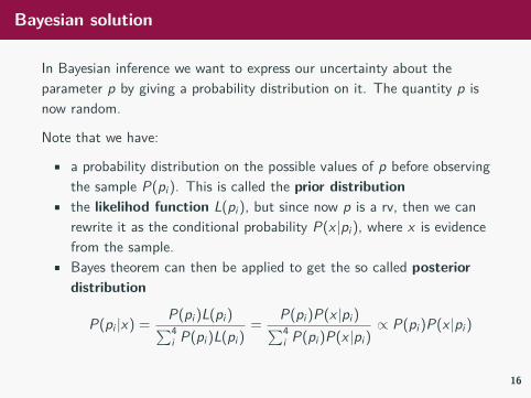
Bayesian solution
In Bayesian inference we want to express our uncertainty about theparameter p by giving a probability distribution on it. The quantity p isnow random.
Note that we have:
• a probability distribution on the possible values of p before observingthe sample P(pi ). This is called the prior distribution
• the likelihod function L(pi ), but since now p is a rv, then we canrewrite it as the conditional probability P(x |pi ), where x is evidencefrom the sample.
• Bayes theorem can then be applied to get the so called posteriordistribution
P(pi |x) = P(pi )L(pi )∑4i P(pi )L(pi )
= P(pi )P(x |pi )∑4i P(pi )P(x |pi )
∝ P(pi )P(x |pi )
16

Bayesian solution
prior <- c(.4, .3, .2, .1)like <- choose(30,x)*p^x*(1-p)^30-xposterior <- prior*like/sum(prior*like); posterior
## [1] 0.01085235 0.52310482 0.44022371 0.02581912
plot(p,posterior,type="h", main="posterior", cex.lab=0.7,cex.axis=0.5, ylab="posterior prob ", ylim=c(0,0.6), col=2)
0.5 0.6 0.7 0.8 0.9
0.0
0.2
0.4
0.6
posterior
p
post
erio
r pr
ob
17

Likelihood vs Bayesian
In the example:
• The likelihood estimate was p = 0.8, Gold, since this is value of theparameter with the highest value of the likelihood.
• In Bayesian inference we have a probability distribution over theparameter space. We can say that the value is p = 0.7 withprobability ≈ 0.52, Extra. This is a probability statement.
• Bayesian approach allows us to update our prior information withexperimental data
information post experiment ∝ information from experiment ×information prior to experiment
posterior ∝ prior×likelihood
18

Introducing Bayesian inference
Bayes theorem: continuos variables
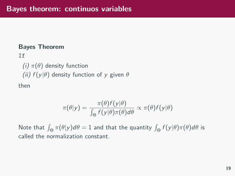
Bayes TheoremIf
(i) π(θ) density function(ii) f (y |θ) density function of y given θ
then
π(θ|y) = π(θ)f (y |θ)∫Θ f (y |θ)π(θ)dθ
∝ π(θ)f (y |θ)
Note that∫
Θ π(θ|y)dθ = 1 and that the quantity∫
Θ f (y |θ)π(θ)dθ iscalled the normalization constant.
19

Bayesian paradigm: model and likelihood
Consider a model, a family of probability distributions indexed by aparameter θ among which we assume there is the distribution of y :
f (y |θ), θ ∈ Θ.
This is no different than the classical paradigm, but for the fact that thedistributions are defined conditional on the value of the parameter (whichis not a r.v. in the classical setting)
One defines then the likelihood
L(θ; y) ∝ f (y |θ),
as in the classical paradigm.
20

Bayesian paradigm: prior distribution
A prior distribution is set on the parameter θ
π(θ)
which is independent of observations (it is called prior since it comesbefore observation).
This is the new thing
Prior information and likelihood are combined in Bayes’ theorem to givethe posterior distribution
π(θ|y) = π(θ)f (y |θ)∫Θ f (y |θ)π(θ)dθ
∝ π(θ)f (y |θ) ∝ π(θ)L(θ; y)
which sums up all the information we have on the parameter θ.
21

Inference on the quality of seeds
We are again interested in estimating the proportion of high quality seedsin the boxes. But now we assume that the proportion p can be any valuein the interval [0, 1]. We still have a sample of n seeds drawn from a box(with replacement), and we count the number of high quality seeds x .
We want to infer on the value p. Data are i.i.d realizations from a Be(p).
We can never know the real value of p, unless we can rely on a samplewhere n→∞.
We can design a procedure that selects values of p that are moresupported by the data. We can then judge how uncertain is our procedureby looking at its behaviour in possible (not actual) replication of thesample under the same condition. Classical inference
We can try to give a probability distribution over possible values of theparameter p. And this probability distribution will summarize all theinformation we have about it: before and after observing the data.Bayesian inference 22

Estimating p
1. Likelihood estimation is straightforward:
• L(p) ∝ px (1− p)n−x
• it is easy to show that ML estimate is p = x/n. The observedproportion of high quality seeds in the sample.
2. Bayesian solution requires specification of the probability distributionπ(p).
• Since p ∈ [0, 1] candidates are probability models whose support isthe interval [0, 1].
• Random variables belonging to the Beta family could be appropriate
23

The likelihood function
n <- 30; z=23;curve(x^z*(1-x)^(30-z), xlim=c(0,1), xlab="p",ylab="L(p)")
0.0 0.2 0.4 0.6 0.8 1.0
0e+
004e
−08
8e−
08
p
L(p)
24

The Beta distributions
π(θ) = Γ(α + β)Γ(α)Γ(β)θ
α−1(1− θ)β−1
where 0 < θ < 1 and α, β > 0,
E (θ) = α
α + β, V (θ) = αβ
(α + β)2(α + β + 1)
remind that Γ(x) =∫ +∞
0 tx−1etdt and if x is integer Γ(x) = (x − 1)!
25

The Beta distributions
0.0 0.2 0.4 0.6 0.8 1.0
0.0
0.5
1.0
1.5
2.0
2.5
α=β
p
π(p)
0.0 0.2 0.4 0.6 0.8 1.0
01
23
4
α>β
p
π(p)
26
The posterior distribution
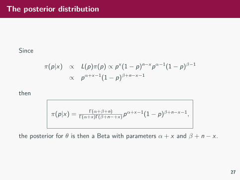
Since
π(p|x) ∝ L(p)π(p) ∝ px (1− p)n−x pα−1(1− p)β−1
∝ pα+x−1(1− p)β+n−x−1
then
π(p|x) = Γ(α+β+n)Γ(α+x)Γ(β+n−+x) pα+x−1(1− p)β+n−x−1,
the posterior for θ is then a Beta with parameters α + x and β + n − x .
27

Likelihood, prior and posterior
Assume that in our case we believe, before getting the sample, that valuesabove 0.5 are more likely. I could use as a prior a Beta(7,4) whose mean is7/11=0.636. Note that the likelihood (normalized so that it integrate to1) is also a Beta with parameters (24,8).
Then the posterior is still a Beta(30,11)
0.0 0.2 0.4 0.6 0.8 1.0
01
23
45
6
p
dens
ity
priorlikelihoodposterior
28

Likelihood and Bayesian inference
A statistical problem is faced when, given observations, we want to assesswhat random mechanism generated them
• In other words,• there are two or more probability distributions which may have
generated the observations;• analyzing the data we want to infer on the actual distribution which
generated the data (or on some property of it).• How? Let us discriminate between the two approaches.
• Based on the likelihood we compare P(Data|Model) for the differentmodels.
• In Bayesian statistics comparing P(Model |Data).
In the likelihood approach quality of the procedure is evaluated relyingupon fictitious repetitions of the experiment.
29

Classical and Bayesian statistical inference, differences
In CLASSICAL INFERENCE
• the conclusion is not derived within probability calculus rules (theseare used in fact, but the conclusion is not a direct consequence)
• the likelihood and the probability distribution of the sample are used;• the parameter is a constant.
In BAYESIAN INFERENCE
• the reasoning and the conclusion is an immediate consequence ofprobability calculus rules (more specifically of Bayes’ theorem);
• the likelihood and the prior distribution are used;• the parameter is a random variable.
30

Bayesian vs classical inference
In the Bayesian approach the parameter is random: this is a fundamentaldifference between the two approaches, how can this be interpreted?
• In classical statistics, on the contrary, the parameter is a fixedquantity.
• The random character of θ represents our ignorance on it.• Random means, in this context, not known for lack of information.
We measure our uncertainty about the model• The randomness and the probability distribution on θ are subjective.• The probability in Bayesian approach is a subjective probability, i.e.,
the probability of a given event is defined as the “degree of belief ofthe subject on the event”.
31

The role of subjective probability
• Consider events such as tail is observed when a coin is thrown,• everyone (presumably) would agree on the value of the probability;• the frequentist definition is intuitively applied;• → this is an ‘objective’ probability.
• For events such as Juventus will be Italian champion next year orRight wing parties will win next elections,
• it is still possible to state a probability;• everyone would assign a different probability;• the probability given by someone will change in time depending on
avalaible information.
One then accepts that the probability is not an objective property of aphenomenon but rather the opinion of a person and one defines
Subjective probability: definition (de Finetti)The probability of an event is, for an individual, his degree of belief on theevent.
32

Bayesian statistics and subjective probability
If the probability is a subjective degree of belief, it depends on theinformation which is subjectively available, and that by random we meannot known for lack of information.
The subjective definition of probability is most compatible with theBayesian paradigm, in which:
• the parameter to be estimated is a well specified quantity but is notknown for lack of information
• a probability distribution is (subjectively) specified for the parameterto be estimated, this is called a priori
• after seeing experimental results the probability distribution on theparameter is updated using Bayes’ theorem to combine experimentalresults (likelihood) and the prior to obtain the posterior distribution.
Note that, starting in 1763 (the year Bayes’ theorem was published),Bayesian statistics comes first, before the so–called classical statistics,initially developed by Galton and Pearson at the end of XIX century andthen by Fisher in the twenties. 33