Bayesian Canonical Correlation Analysis - Research

Journal of Machine Learning Research 14 (2013) 965-1003 Submitted 7/12; Revised 1/13; Published 4/13

Bayesian Canonical Correlation Analysis

Arto Klami [email protected]

Seppo Virtanen [email protected]

Samuel Kaski∗ [email protected]

Helsinki Institute for Information Technology HIIT

Department of Information and Computer Science

PO Box 15600

Aalto University

00076 Aalto, Finland

Editor: Neil Lawrence

Abstract

Canonical correlation analysis (CCA) is a classical method for seeking correlations between two

multivariate data sets. During the last ten years, it has received more and more attention in the

machine learning community in the form of novel computational formulations and a plethora of

applications. We review recent developments in Bayesian models and inference methods for CCA

which are attractive for their potential in hierarchical extensions and for coping with the combina-

tion of large dimensionalities and small sample sizes. The existing methods have not been partic-

ularly successful in fulfilling the promise yet; we introduce a novel efficient solution that imposes

group-wise sparsity to estimate the posterior of an extended model which not only extracts the

statistical dependencies (correlations) between data sets but also decomposes the data into shared

and data set-specific components. In statistics literature the model is known as inter-battery factor

analysis (IBFA), for which we now provide a Bayesian treatment.

Keywords: Bayesian modeling, canonical correlation analysis, group-wise sparsity, inter-battery

factor analysis, variational Bayesian approximation

1. Introduction

Canonical correlation analysis (CCA), originally introduced by Hotelling (1936), extracts linear

components that capture correlations between two multivariate random variables or data sets. Dur-

ing the last decade the model has received a renewed interest in the machine learning community

as the standard model for unsupervised multi-view learning settings. In a sense, it is the analogue

of principal component analysis (PCA) for two co-occurring observations, or views, retaining the

positive properties of closed-form analytical solution and ease of interpretation of its more popular

cousin.

A considerable proportion of the work has been on non-linear extensions of CCA, including

neural network based solutions (Hsieh, 2000) and kernel-based variants (Bach and Jordan, 2002;

Lai and Fyfe, 2000; Melzer et al., 2001). This line of research has been covered in a comprehensive

overview by Hardoon et al. (2004), and hence will not be discussed in detail in this article. Instead,

we review a more recent trend treating CCA as a generative model, initiated by the work of Bach and

∗. Is also at Helsinki Institute for Information Technology HIIT, Department of Computer Science, University of

Helsinki, Finland.

c©2013 Arto Klami, Seppo Virtanen and Samuel Kaski.

KLAMI, VIRTANEN AND KASKI

Jordan (2005). Most works in the generative approach retain the linear nature of CCA, but provide

inference methods more robust than the classical linear algebraic solution and, more importantly,

the approach leads to novel models through simple changes in the generative description or via the

basic principles of hierarchical modeling.

The generative modelling interpretation of CCA is essentially equivalent to a special case of a

probabilistic interpretation (Browne, 1979) of a model called inter-battery factor analysis (IBFA;

Tucker, 1958). While the analysis part of Browne (1979) is limited to the special case of CCA, the

generic IBFA model describes not only the correlations between the data sets but provides also com-

ponents explaining the linear structure within each of the data sets. One way of thinking about IBFA

is that it complements CCA by providing a PCA-like component description of all the variation not

captured by the correlating components. If the analysis focuses on only the correlating compo-

nents, or equivalently the latent variables shared by both data sets, the solution becomes equivalent

to CCA. However, the extended model provides novel application opportunities not immediately

apparent in the more restricted CCA model.

The IBFA model has recently been re-invented in the machine learning community by several

authors (Klami and Kaski, 2006, 2008; Ek et al., 2008; Archambeau and Bach, 2009), resulting in

probabilistic descriptions identical with that of Browne (1979). The inference has been primarily

based on finding the maximum likelihood or maximum a posteriori solution of the model, with

practical algorithms based on expectation maximization. Since the terminology of calling these

models (probabilistic) CCA has already become established in the machine learning community,

we will regard the names CCA and IBFA interchangeable. Using the term CCA emphasizes finding

of the correlations and shared components, whereas IBFA emphasizes the decomposition into shared

and data source-specific components.

In this paper we extend this IBFA/CCA work to a fully Bayesian treatment, extending our

earlier conference paper (Virtanen et al., 2011), and in particular provide two efficient inference

algorithms, a variational approximation and a Gibbs sampler, that automatically learn the structure

of the model that is, in the general case, unidentifiable. The model is solved as a generic factor

analysis (FA) model with a specific group-wise sparsity prior for the factor loadings or projections,

and an additional constraint tying the residual variances within each group to be the same. We

demonstrate how the model not only finds the IBFA solution, but also provides a CCA solution

superior to the earlier Bayesian variants of Klami and Kaski (2007) and Wang (2007).

The technical description of the model and its connection to other models are complemented

with demonstrations on practical application scenarios for the IBFA model. The main purpose of

the experiments is to show that the tools find the intended solution, and to introduce prototypical

application cases.

2. Canonical Correlation Analysis

Before explaining the Bayesian approach for canonical correlation analysis (CCA), we briefly in-

troduce the classical CCA problem. Given two co-occurring random variables with N observations

collected as matrices X1 ∈RD1×N and X2 ∈R

D2×N , the task is to find linear projections U ∈RD1×K

and V∈RD2×K so that the correlation between uTk X(1) and vT

k X(2) is maximized for the components

k, under the constraint that uTk X(1) and uT

k′X(1) are uncorrelated for all k 6= k′ (and similarly for the

966

BAYESIAN CANONICAL CORRELATION ANALYSIS

other view). The solution can be found analytically by solving the eigenvalue problems

C−111 C12C−1

22 C21u = ρ2u, (1)

C−122 C21C−1

11 C12v = ρ2v,

where

C =

[

C11 C12

C21 C22

]

is the joint covariance matrix of x(1) and x(2) and ρ denotes the canonical correlation. In practice

all components can be found by solving a single generalized eigenvalue problem. For more detailed

discussion on classical CCA, see for instance the review of Hardoon et al. (2004).

3. Model

Our Bayesian approach to CCA is based on latent variable models and linear projections. At the

core of the generative process is an unobserved latent variable z ∈ RK×1, which is transformed

via linear mappings to the observation spaces to represent the two multivariate random variables

x(1) ∈ RD1×1 and x(2) ∈ R

D2×1. The observed data samples are provided as matrices X(m) =

[x(m)1 , ...,x

(m)N ] ∈ R

Dm×N with N observations. To simplify the notation, we denote by x = [x(1);x(2)]and X= [X(1);X(2)] the feature-wise concatenation of the two random variables. Throughout the pa-

per we use the superscript (m), where m is 1 or 2, to denote the view or data set in question, though

for scalar variables (such as Dm) we use the subscript without risk of confusion to streamline the

notation. For matrices and vectors the subscripts are used to indicate the individual elements, with

X:,n denoting the whole nth column of X (also denoted by xn to simplify the notation when appro-

priate) and Xd,: denoting the dth row treated as a column vector. Finally, we use 0 and I to denote

zero- and identity matrices of sizes which make sense in the context, without cluttering the notation.

3.1 Inter-battery Factor Analysis

In the latent variable model studied in this work,

z∼ N(0,I),

z(m) ∼ N(0,I), (2)

x(m) ∼ N(A(m)z+B(m)z(m),Σ(m)),

following the probabilistic interpretation of inter-battery factor analysis by Browne (1979).1 The

notation N(µ,Σ) corresponds to the normal distribution with mean µ and covariance Σ. Here the

Σ(m) ∈ R

Dm×Dm are diagonal matrices, indicating independence of the noise over the features. Our

practical solutions will further simplify the model by assuming isotropic noise, but could easily be

extended to generic diagonal noise covariances as well. A plate diagram of the model is given in

Figure 1.

The conceptual meaning of the various terms in the model is as follows. The shared latent vari-

ables z capture the variation common to both data sets, and they are transformed to the observation

1. The original definition by Browne (1979) allows for more relaxed definitions for the various covariance terms, but in

practice he resorts to the choices made above in the actual analysis part of his work and makes the same independence

assumptions.

967


K

NK1 K2

Σ(1)

b(1)

z(1)

a(1)

x(1)

z

a(2)

x(2)

z(2)

b(2)

Σ(2)

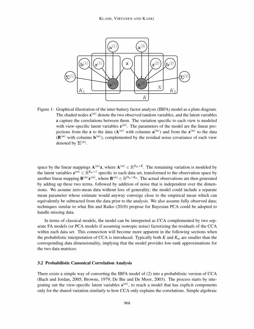
Figure 1: Graphical illustration of the inter-battery factor analysis (IBFA) model as a plate diagram.

The shaded nodes x(m) denote the two observed random variables, and the latent variables

z capture the correlations between them. The variation specific to each view is modeled

with view-specific latent variables z(m). The parameters of the model are the linear pro-

jections from the z to the data (A(m) with columns a(m)) and from the z(m) to the data

(B(m) with columns b(m)), complemented by the residual noise covariance of each view

denoted by Σ(m).

space by the linear mappings A(m)z, where A(m) ∈ RDm×K . The remaining variation is modeled by

the latent variables z(m) ∈ RKm×1 specific to each data set, transformed to the observation space by

another linear mapping B(m)z(m), where B(m) ∈RDm×Km . The actual observations are then generated

by adding up these two terms, followed by addition of noise that is independent over the dimen-

sions. We assume zero-mean data without loss of generality; the model could include a separate

mean parameter whose estimate would anyway converge close to the empirical mean which can

equivalently be subtracted from the data prior to the analysis. We also assume fully observed data;

techniques similar to what Ilin and Raiko (2010) propose for Bayesian PCA could be adopted to

handle missing data.

In terms of classical models, the model can be interpreted as CCA complemented by two sep-

arate FA models (or PCA models if assuming isotropic noise) factorizing the residuals of the CCA

within each data set. This connection will become more apparent in the following sections when

the probabilistic interpretation of CCA is introduced. Typically both K and Km are smaller than the

corresponding data dimensionality, implying that the model provides low-rank approximations for

the two data matrices.

3.2 Probabilistic Canonical Correlation Analysis

There exists a simple way of converting the IBFA model of (2) into a probabilistic version of CCA

(Bach and Jordan, 2005; Browne, 1979; De Bie and De Moor, 2003). The process starts by inte-

grating out the view-specific latent variables z(m), to reach a model that has explicit components

only for the shared variation similarly to how CCA only explains the correlations. Simple algebraic

968


manipulation gives the model

z∼ N(0,I),

x(m) ∼ N(A(m)z,B(m)B(m)T

+Σ(m)).

The latent representation of this model is simpler, only containing the z instead of three separate sets

of latent variables, but the diagonal covariance of the IBFA model is replaced with B(m)B(m)T

+Σ(m).

In effect, the view-specific variation is now modeled only implicitly, in form of correlating noise. If

we further assume that the dimensionality of the z(m) is sufficient for modeling all such variation,

the model can be re-parameterized with Ψ(m) = B(m)B(m)T

+Σ(m) without loss of generality. This

results in the model

z∼ N(0,I),

x(m) ∼ N(A(m)z,Ψ(m)), (3)

where Ψ(m) is a generic covariance matrix. This holds even if assuming isotropic noise in (2).

Browne (1979) proved that (3) is equivalent to classical CCA, by showing how the maximum

likelihood solution finds the same canonical weights as regular CCA, up to a rotation. Bach and

Jordan (2005) proved the same result through a slightly different derivation, whereas De Bie and

De Moor (2003) provided a partial proof showing that the CCA solution is a stationary point of the

likelihood. The fundamental result of these derivations is that the maximum likelihood estimates

A(m) correspond to rank-preserving linear transformations of U and V, the solutions of (1). While

the connection was shown for the case with a generic Ψ, it holds also for the IBFA model as long as

the rank of B(m) is sufficient for modeling all data set-specific variation. This is because the model

itself is the same, it just explicitly includes the nuisance parameters z(m) and B(m).

Even though the generative formulation is equivalent to classical CCA in the sense that they both

find the same subspace, one difference pointed out also by Browne (1979) is worth emphasizing:

The generative formulation maintains a single latent variable z that captures the shared variation,

whereas CCA results in two separate but correlating variables obtained by projecting the observed

variables into the correlating subspace. It is, however, possible to move between these representa-

tions; a single latent variable can be obtained by averaging the canonical scores (uTk X(1) and vT

k X(2))

of regular CCA; two separate latent variables can be produced with the generative formulation by

estimating the distribution of z conditional on having observed only one of the views (p(z|x(1)) and

p(z|x(2))).

3.3 Identifiability

The model in (2) is in general unidentifiable in two respects. The first is shared with the marginalized

version in (3): the models are invariant to rank-preserving linear transformations. For all invertible

R ∈RK×K we have A(m)z = A(m)RR−1z, and hence the solution is defined only up to such transfor-

mations. In other words, the model finds the same subspace as the classical CCA would, but extract-

ing the specific components requires further constraints or postprocessing. Browne (1979) resorts

to simple identifiability constraints borrowed from regular factor analysis, whereas Archambeau

et al. (2006) provide a post-processing step that is close to applying regular CCA to the covariance

matrices of the probabilistic solution.

969


The full IBFA model (2) has additional degrees of freedom in terms of component allocation.

The model comes with three separate sets of latent variables with component numbers K, K1 and

K2. However, individual components can be moved between these sets without influencing the

likelihood of the observed data; removal of a shared component can always be compensated by

introducing two view-specific components, one for each data set, that have the same latent variables.

In practice, all solutions for the full IBFA model hence need to carefully address the choice of model

complexity. In the next section we will introduce one such solution, based on Bayesian inference.

3.4 The Role of View-specific Variation

The models (2) and (3) are both very closely related to probabilistic formulation of PCA, FA, and

many other simple matrix factorizations. The crucial difference worth pointing out is the definition

of the noise. Instead of assuming independent noise over the dimensions the CCA model allows

for arbitrary correlations between them. This is done either by explicitly parameterizing the noise

through a covariance matrix Ψ(m) as in (3) or by the separate view-specific components B(m)z(m) as

in (2).

Modeling the correlations in view-specific noise is crucial for extracting the true correlations

between the views. This is easy to illustrate by constructing counter-examples where the correlating

dimensions are of smaller scale than some strong view-specific variation. Any joint model assuming

independent noise over the dimensions will find the view-specific variation as the most prominent

components. It may be possible to identify these components as view-specific in a post-processing

step to reach interpretation similar to CCA, but directly modeling the view-specific variation as

separate components has obvious advantages.

The importance of modeling the variation within each view in addition to the shared effects is

so subtle that even some authors claiming to work with CCA have ignored it. For example, Shon

et al. (2006), Fujiwara et al. (2009), and Rai and Daume III (2009) all describe their models as

CCA, but eventually resort to assuming independent noise on top of the shared components. This is

a reasonable assumption that simplifies computation dramatically, but it also means that the models

do not correspond to CCA but are instead variants of collective matrix factorization (CMF; Singh

and Gordon 2008). They are useful tools for multi-view data, but it is important to realize that the

simplifying assumption dramatically changes the nature of the model. In particular, such models

are likely to misinterpret strong view-specific variation as a shared effect, since they have no means

of explaining it otherwise. Our choice of modeling the view-specific variation as a low-rank process

results in similar computational performance as ignoring the view-specific variation, but retains the

capability of modeling also view-specific variation.

4. Inference

For learning the IBFA model we need to infer both the latent signals z and z(m) as well as the linear

projections A(m) and B(m) from data. For this purpose, we need to estimate the posterior distribution

p(z,z(1),z(2),A(1),A(2),B(1),B(2),Σ(1),Σ(2)|X(1),X(2)), and marginalize over the possibly uninter-

esting variables. In this section we first review the earlier inference solutions for the Bayesian CCA

model without presenting the technical details, and then proceed to explaining our solution for the

full Bayesian IBFA model.

Before explaining the Bayesian inference solutions, we mention earlier maximum likelihood

solutions for completeness. Bach and Jordan (2005) gave an expectation maximization algorithm

970


for the pure CCA model, whereas Klami and Kaski (2008) extended it for the IBFA model. Both

approaches generalize immediately to seeking maximum a posteriori (MAP) estimates, which pro-

vides a justified way for adding regularization in the solution. Here, however, we are interested in

analysis of the full posterior distribution.

4.1 Bayesian Inference

For Bayesian analysis, the model needs to be complemented with priors for the model parameters.

Bayesian treatments of CCA were independently proposed by Klami and Kaski (2007) and Wang

(2007). Both formulations use the inverse-Wishart distribution as a prior for the covariance matrices

Ψ(m) in (3) and apply the automatic relevance determination (ARD; Neal, 1996) prior for the linear

mappings A(m).

The ARD is a Normal-Gamma prior for the projection weights. For each component (column)

a(m)k the prior specifies a precision α

(m)k that controls the scale of the values for that component:2

ARD(A(m)|α0,β0) =K

∏k=1

p(a(m)k |α

(m)k )p(α

(m)k |α0,β0),

α(m)k ∼ Gamma(α0,β0),

a(m)k ∼ N(0,(α

(m)k )−1I).

The hyperpriors α0,β0 are set to small values (in our experiments to α0 = β0 = 10−14) to obtain

a relatively noninformative prior with wide support.3 The posterior of the model then becomes

one where the number of components is automatically selected by pushing α(m)k of unnecessary

components towards infinity. A justification for this observation is obtained by integrating α(m)k

out in the above prior; we then get a heavy-tailed prior for the elements of A(m) with considerable

posterior mass around zero. The component choice can be made more robust by further assuming

α(1) = α

(2), which corresponds to placing the ARD prior for A = [A(1);A(2)] (Klami and Kaski,

2007). More data will then be used for determining the activity of each component, but data sets

with comparable scale are required. Further insights into the ARD prior are provided by Wipf and

Nagarajan (2008).

For the covariance matrices Ψ(m) a natural choice is to use a conjugate inverse-Wishart prior

Ψ(m) ∼ IW(S0,ν0)

with ν0 degrees of freedom and scale matrix S0, which results in positive definite draws as long as

the degrees of freedom (which for N samples becomes N +ν0 in the posterior) is at least equal the

data dimensionality. Both Klami and Kaski (2007) and Wang (2007) adopted this choice.

Given the above priors, several inference techniques for the posterior are feasible. Wang (2007)

provided a variational mean-field algorithm, whereas Klami and Kaski (2007) used Gibbs sampling.

Both of these algorithms are fairly straightforward and easy to derive, since all conditional distribu-

tions are conjugate. The former is more efficient in determining the correct model complexity due

2. Note that ARD generates both the matrix A(m) as well as the scales α(m), and hence notation ARD(A(m),α(m)|α0,β0)would be more accurate. However, since α

(m) is irrelevant for the rest of the model, we adopt the more compact

notation.

3. The distribution is flat over the positive real line, but slightly favors values near zero.

971


to the ARD prior updates being more efficient in the variational framework, whereas the latter is

easier to extend, as demonstrated by Klami and Kaski (2007) by using the Bayesian CCA as part of

a non-parametric hierarchical model. Further extensions of the CCA model, described in Section 6,

have used both approaches.

Despite the apparent simplicity of the derivation, it is worth pointing out that inference of the

Bayesian CCA model is difficult for large dimensionalities. This is because we need to estimate the

posterior distribution over the Dm×Dm covariance matrices Ψ(m). The inference algorithms gener-

ally need to invert those matrices in every step, resulting in O(D3m) complexity. More importantly,

providing accurate estimates would require extremely large sample sizes; the covariance matrix has

O(D2m) parameters, which is often well above the data set size. Hence the direct Bayesian treatment

of CCA needs to resort to either using very strong priors (for example, favoring diagonal covariance

matrices and hence regularizing the model towards Bayesian PCA), or it will end up doing infer-

ence over a very wide posterior. Consequently, all the practical applications of Bayesian CCA in the

earlier works have been for relatively low-dimensional data; the original works by Klami and Kaski

(2007) and Wang (2007) had at most 8 dimensions in any of their experiments. Later applications

have typically used some alternative dimensionality reduction techniques to make Bayesian CCA

feasible for otherwise too high-dimensional data (Huopaniemi et al., 2009, 2010).

4.2 Group-wise Sparsity for IBFA

While the above solutions are sufficient for the CCA model, barring the difficulties with high dimen-

sionality, the full IBFA model requires more advanced inference methods. Next we will introduce

a novel inference solution extending our earlier conference paper (Virtanen et al., 2011). Besides

providing a Bayesian inference technique for the IBFA model, the algorithm is applicable also to

the regular CCA case and, as will be shown later, actually is superior to the earlier solutions also for

that scenario.

A main challenge in learning the Bayesian IBFA (BIBFA) model, as discussed in Section 3.3,

is that it requires learning three separate sets of components and the solution is unidentifiable with

respect to allocating components to the three groups. A central element in our solution is to replace

these three sets with just one set, and solve the allocation by requiring the projections to be sparse

in a specific structured way. This is done in a way that does not change the model itself, but allows

automatic complexity selection.

We start with a straightforward re-formatting of the model. We define y = [z;z(1);z(2)] ∈RKc×1,

where Kc = K +K1 +K2, as the concatenation of the three latent variables and set

W =

[

A(1) B(1) 0

A(2) 0 B(2)

]

(4)

and

Σ=

[

Σ(1) 0

0 Σ(2)

]

.

Now we can write (2) equivalently as

y∼ N(0,I),

x∼ N(Wy,Σ). (5)

972


In other words, we are now analyzing the feature-wise concatenation of the data sources with a

single latent variable model with diagonal noise covariance Σ ∈ RD×D, where D = D1 +D2, and a

projection matrix W ∈ RD×Kc with the specific structure shown in (4).

Ignoring the structure in W, the model is actually a Bayesian factor analysis model (Ghahramani

and Beal, 2000). If Σ is further assumed to be spherical (Σ= σ2I), the model equals the Bayesian

PCA (Bishop, 1999) with the specific structure in W. We use Σ(m) = σ2

mI with a Gamma prior

for the noise precisions τm = σ−2m . That is, we make the PCA assumption separately for both data

sets. However, it is important to remember that the model still allows for dependencies between the

features of both views, by modeling them with B(m)z(m). Hence, the spherical noise covariance does

not restrict the flexibility of the model but decreases the number of parameters. Alternatively, we

could allow each dimension to have their own variance parameter as in factor analysis models; this

could be useful when the scales of the variables are very different.

Since efficient inference solutions are available for regular factor analysis, the only challenge in

learning the BIBFA model is in obtaining the right kind of structure for W. We solve the BIBFA

model by doing inference directly for (5) and learn the structure of W by imposing group-wise

sparsity for the components (columns of W), which results in the model automatically converging

to a solution that matches (4) (up to an arbitrary re-ordering of the columns). In other words, we do

not directly specify the matrices A(m) and B(m), but instead learn a single W matrix. To implement

the group-wise sparsity, we divide the variables in x into two groups corresponding to the two data

sets, and construct a prior that encourages sparsity over these groups. For each component wk the

elements corresponding to one group are either pushed all towards zero, or are all allowed to be

active. Recently Jia et al. (2010) introduced a similar sparsity constraint for learning factorized

latent spaces; our approach can be seen as a Bayesian realization of the same idea, applied to

canonical correlation analysis.

It turns out that the correct form of sparsity can easily be obtained by a simple extension of

the ARD prior used for component selection in many Bayesian component models, including the

Bayesian CCA described in the previous section. We define the group-wise ARD as

p(W) =2

∏m=1

ARD(W(m)|α0,β0),

with separate ARD prior for each W(m). Here W(1) denotes the first D1 rows of W and W(2) refers

to the remaining D2 rows. Similarly to how ARD has earlier been used to choose the number of

components, the group-wise ARD makes unnecessary components w(m)k inactive for each of the

views separately. The components needed for modeling the shared response will have small α(m)k

(that is, large variance) for both views, whereas the view-specific components will have small α(m)k

for the active view and a large one for the inactive one. Finally, the model still selects automatically

the total number of components by making both views inactive for unnecessary components. To our

knowledge, Virtanen et al. (2011) is the first to consider this simple extension of ARD into multiple

groups. Later Virtanen et al. (2012a) and Damianou et al. (2012) discussed the prior in more detail,

presenting also extensions to more than two groups.

In practice, the elements of the inactive w(m)k will not become pushed exactly to zero, but instead

to very small values. For most applications of BIBFA this is not a problem, since we need not iden-

tify the components. For example, the demonstration in Section 7.2 that uses CCA for predicting

one view from the other automatically ignores the view-specific components even when w(m)k is not

973


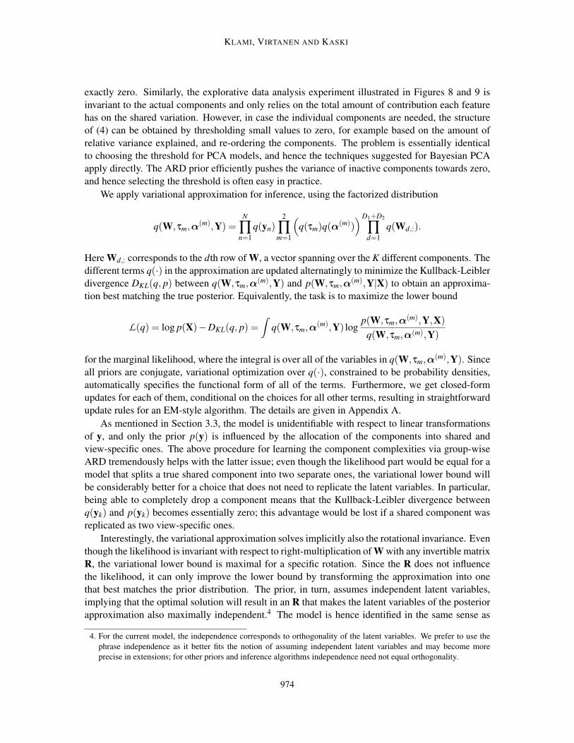
exactly zero. Similarly, the explorative data analysis experiment illustrated in Figures 8 and 9 is

invariant to the actual components and only relies on the total amount of contribution each feature

has on the shared variation. However, in case the individual components are needed, the structure

of (4) can be obtained by thresholding small values to zero, for example based on the amount of

relative variance explained, and re-ordering the components. The problem is essentially identical

to choosing the threshold for PCA models, and hence the techniques suggested for Bayesian PCA

apply directly. The ARD prior efficiently pushes the variance of inactive components towards zero,

and hence selecting the threshold is often easy in practice.

We apply variational approximation for inference, using the factorized distribution

q(W,τm,α(m),Y) =

N

∏n=1

q(yn)2

∏m=1

(

q(τm)q(α(m))

)D1+D2

∏d=1

q(Wd,:).

Here Wd,: corresponds to the dth row of W, a vector spanning over the K different components. The

different terms q(·) in the approximation are updated alternatingly to minimize the Kullback-Leibler

divergence DKL(q, p) between q(W,τm,α(m),Y) and p(W,τm,α

(m),Y|X) to obtain an approxima-

tion best matching the true posterior. Equivalently, the task is to maximize the lower bound

L(q) = log p(X)−DKL(q, p) =∫

q(W,τm,α(m),Y) log

p(W,τm,α(m),Y,X)

q(W,τm,α(m),Y)

for the marginal likelihood, where the integral is over all of the variables in q(W,τm,α(m),Y). Since

all priors are conjugate, variational optimization over q(·), constrained to be probability densities,

automatically specifies the functional form of all of the terms. Furthermore, we get closed-form

updates for each of them, conditional on the choices for all other terms, resulting in straightforward

update rules for an EM-style algorithm. The details are given in Appendix A.

As mentioned in Section 3.3, the model is unidentifiable with respect to linear transformations

of y, and only the prior p(y) is influenced by the allocation of the components into shared and

view-specific ones. The above procedure for learning the component complexities via group-wise

ARD tremendously helps with the latter issue; even though the likelihood part would be equal for a

model that splits a true shared component into two separate ones, the variational lower bound will

be considerably better for a choice that does not need to replicate the latent variables. In particular,

being able to completely drop a component means that the Kullback-Leibler divergence between

q(yk) and p(yk) becomes essentially zero; this advantage would be lost if a shared component was

replicated as two view-specific ones.

Interestingly, the variational approximation solves implicitly also the rotational invariance. Even

though the likelihood is invariant with respect to right-multiplication of W with any invertible matrix

R, the variational lower bound is maximal for a specific rotation. Since the R does not influence

the likelihood, it can only improve the lower bound by transforming the approximation into one

that best matches the prior distribution. The prior, in turn, assumes independent latent variables,

implying that the optimal solution will result in an R that makes the latent variables of the posterior

approximation also maximally independent.4 The model is hence identified in the same sense as

4. For the current model, the independence corresponds to orthogonality of the latent variables. We prefer to use the

phrase independence as it better fits the notion of assuming independent latent variables and may become more

precise in extensions; for other priors and inference algorithms independence need not equal orthogonality.

974


Rotation No rotation

100

200

300

400

500

Itera

tions

Rotation No rotation

−13

460

−13

400

Low

er b

ound

Figure 2: Illustration of the effect of parameter-expanded VB, where the variational lower bound

is explicitly optimized with respect to a linear transformation R to make the updates

less correlated. The number of iterations until convergence is reduced clearly when op-

timizing for the rotation (left), while the lower bound is still on average slightly better

(right). However, since R is optimized numerically the total computation time might still

be smaller without the rotation optimization, depending on the data and parameter values

(such as Kc). These plots were drawn for the data analyzed in Section 7.1.1 and Figure 9;

the boxplots show the results of 50 runs with random initialization. The overall picture is

similar for other data sets, but the actual differences vary depending on the complexity of

the data. In practice, we recommend trying both with and without the rotation for each

data type, and to choose the solution resulting in a better lower bound.

the classical CCA solution is; the latent variables are assumed orthogonal, instead of assuming

orthogonal projections (like in PCA).

That property also allows deriving a more efficient algorithm for optimizing the variational

approximation, following the idea of parameter-expanded variational Bayes (Qi and Jaakkola, 2007;

Luttinen and Ilin, 2010). We introduce explicit parameter R ∈ RKc×Kc in the approximation and

optimize the lower bound also with respect to it. Transforming the parameters with R improves

the convergence speed dramatically, due to lower correlations between the EM updates for y and

W, and often also results in slightly better lower bound. Both of the properties are illustrated in

Figure 2, and the details for how the rotation can be optimized are given in Appendix B.

In summary, the above model formulation with the associated variational approximation pro-

vides a fully Bayesian treatment for the IBFA model. It can also be used for solving the CCA

problem with a low-rank assumption for the view-specific noise. The model automatically se-

lects the complexity of the three separate component types through a group-wise ARD prior ap-

plied for a joint FA model (that additionally shares the noise variances for all variables within a

view), and disambiguates between different rotations by maximizing the orthogonality of the latent

variables for improved interpretability and computational efficiency. Open-source implementation

of the model, written in the R language, is available in CRAN: http://cran.r-project.org/

package=CCAGFA.

975


4.3 On the Choice of Group-sparsity Prior

The above derivation uses group-wise ARD for inferring the component activities. This particular

choice is, however, not the only possibility. In fact, any reasonable prior that results in group-wise

sparse projection matrix W could be adopted. Here we briefly discuss possible alternatives, and

derive one practical implementation that uses sampling-based inference instead of the variational

approximation described above.

BIBFA is essentially a linear model for the concatenation of the two sources, made interpretable

by the group-wise sparsity. Hence, a sufficient requirement for a model to implement the BIBFA

concept is that it can make W:,k sparse in the specific sense of favouring solutions where all of the

elements corresponding to the first D1 or the last D2 dimensions (or both) are driven to zero. This

can be achieved in two qualitatively different ways, called weak and strong sparsity by Mohamed

et al. (2012). The ARD prior is an example of the former, a continuous sparsity-inducing prior

that results in elements that are close to zero but not exactly so. Other priors that induce weak

sparsity could also be considered, such as the group-wise extensions of the Laplace and scale-

mixture priors Archambeau and Bach (2009) and Guan and Dy (2009) used for sparse PCA, but as

we will demonstrate in the empirical experiments, already the ARD prior works well. Hence, we use

it as a representative of weak sparsity priors. As general properties, such priors allow continuous

inference procedures that are often efficient, but it is not always trivial to separate low-activity

components from inactive ones for interpretative purposes. This is because the elements are not

made exactly zero even for the components deemed inactive, but instead the values are pushed to

very small values.

In our applications in Section 7, we do not need to accurately identify the active components,

since already near-zero effects become irrelevant for the predictive measures used. In case more

precise determination of the active components is needed, it may be better to switch to strong spar-

sity, using priors that provide exact zeroes in W. For this purpose, we here extend the element-wise

sparse factor analysis model of Knowles and Ghahramani (2011) for the BIBFA setup. The orig-

inal model is based on the spike-and-slab prior, where each element of W is drawn from a two-

component prior. One of the components, the spike, is a delta distribution centered at zero, whereas

the other, the slab, is a Gaussian distribution. Hence, each element can either become exactly zero

or is drawn from a relatively noninformative distribution. To create a BIBFA method based on this

idea, we introduce the group-wise spike-and-slab prior with the prior

p(W,H,αb,π|α0,β0) = p(π)p(H|π)2

∏m=1

p(W(m)|Hm,:,α(m))p(α(m)|α0,β0), (6)

W(m)d,k |Hm,k,α

(m)k ∼Hm,kN(0,(α

(m)k )−1)+(1−Hm,k)δ0,

Hm,k|πm ∼ Bernoulli(πm),

πm ∼ Beta(1,1),

α(m)k |α0,β0 ∼ Gamma(α0,β0),

where δ0 denotes a point-density at zero. That is, the view-specific πm tells the probability for a

component to be active, binary Hm,k drawn from the Bernoulli distribution tells whether component

k is active in view m, and finally W:,k is either exactly zero or its elements are all drawn indepen-

dently from a Gaussian distribution with precision α(m)k depending on whether Hm,k is zero or one,

respectively.

976


For inference, we use Gibbs sampler by Knowles and Ghahramani (2011) with small modifi-

cations. In particular, the elements of H now depend on Dm features instead of just a single one.

This, however, does not make the inference more complicated; the dimensions are independent and

hence we get the conditional density by multiplying element-wise terms that still integrate W(m)d,k

out. Another change is motivated by the fact that we only need to estimate a 2×K matrix H, in-

stead of a D×K matrix needed for element-wise sparsity. Since we only have two choices for each

component, it does not make sense to use the Indian Buffet Process (IBP) prior for H; there cannot

be any interesting structure in H. Hence, we simplify the model to merely draw each entry of H

independently. The details of the resulting sampler are presented in Appendix D.

4.4 Model Summary

We will next briefly summarize the Bayesian CCA model and lay out the two alternative inference

strategies. These methods will be empirically demonstrated and compared in the following sections.

4.4.1 BAYESIAN CCA WITH LOW-RANK COVARIANCE, OR BAYESIAN IBFA (BIBFA)

The assumption of low-rank covariance results in the IBFA model of (5). Efficient inference is

done in the factor analysis model for x = [x(1);x(2)] with group-wise sparsity prior for the projection

matrix:

y∼ N(0,I),

x∼ N(Wy,Σ), (7)

W(m) ∼ ARD(α0,β0).

Here W(m) denotes the dimensions (rows) of W corresponding to the mth view, and Σ is a diagonal

matrix with D1 copies of τ−11 and D2 copies of τ−1

2 on its diagonal. The noise precision parameters

are given Gamma priors τm ∼ Gamma(ατ0,β

τ0). Inference for the model is done according to the

updates provided in Appendices A and B.

An alternative inference scheme replaces the above ARD prior with the group-wise spike-and-

slab prior of (6) and draws samples from the posterior using Gibbs sampling.

4.4.2 BAYESIAN CCA WITH FULL COVARIANCE (BCCA)

The Bayesian CCA as presented by Wang (2007) and Klami and Kaski (2007) models the view-

specific variation with a free covariance parameter. The full model is specified as

z∼ N(0,I),

x(m) ∼ N(A(m)z,Ψ(m)), (8)

A(m) ∼ ARD(α0,β0),

Ψ(m) ∼ IW(S0,ν0),

and inference follows the variational updates provided by Wang (2007). When A = [A(1);A(2)] is

drawn from a single ARD prior, the lower bound can analytically be optimized with respect to a

rotation R (see Appendix C), resulting in considerable speedup.

977


The variational approximations for both BCCA and BIBFA are deterministic and will converge

to a local optimum that depends on the initialization. We initialize the model by sampling the latent

variables from the prior, and recommend running the algorithm multiple times and choosing the

solution with the best variational lower bound. In the experiments we used 10 initializations.

All of the above require pre-specifying the number of components K. However, since the ARD

prior (or the spike-and-slab prior for the Gibbs sampler variant) automatically shuts down compo-

nents that are not needed, the parameter can safely be set large enough; the only drawback of using

too large K is in increased computation time. In practice, one can follow a strategy where the model

is first run with some reasonable guess for K. In case all components remain active, try again with

a larger K.

5. Illustration

In this section we demonstrate the BIBFA model on artificial data, in order to illustrate the factoriza-

tion into shared and data set-specific components, as well as to show that the inference proceduree

converge to the correct solution. Furthermore, we provide empirical experiments demonstrating

the importance of making the low-rank assumption for the view-specific noise, in terms of both

accuracy and computational speed, by comparing BIBFA (7) with BCCA (8).

The results are illustrated primarily from the point-of-view of the variational inference solution;

the variational approximation is easier to visualize and compare with alternative methods. The

Gibbs sampler produced virtually identical results for these examples, as demonstrated in Figures 4

and 6.

5.1 Artificial Example

First, we validate the model on artificial data drawn from a model from the same model family, with

parameters set up so that it contains all types of components (view-specific and shared components).

The latent signals y were manually constructed to produce components that can be visually matched

with the true ones for intuitive assessment of the results. Also the α(m) parameters, controlling the

activity of each latent component in both views, were manually specified. The projections W were

then drawn from the prior, and noise with fixed variance was added to the observations.

The left column of Figure 3 illustrates the data generation, showing the four latent components,

two of which are shared between the two views. We generated N = 100 samples with D1 = 50

and D2 = 40 dimensions, and applied the BIBFA model with K = 6 components to show that it

learns the correct latent components and automatically discards the excess ones. The results of

the variational inference are shown in the middle column of Figure 3; the Gibbs sampler produces

virtually indistinguishable results. The learned matrix of α-values (and the corresponding elements

in W) reveals that the model extracted exactly four components, correctly identifying two of them

as shared components and two as view-specific ones (one for each data set). The actual latent

components also correspond to the ones used for generating the data. The components are presented

in the order returned by the model, which is invariant to the order. We also see how the model is

invariant to the sign of y, but that it gives the actual components instead of a linear combination of

those, demonstrating that the variational approximation indeed solves the rotational disambiguity

that would remain for instance in the maximum likelihood solution.

The BIBFA results are further illustrated in Figure 4. The plot shows the approximate posterior

for two of the model parameters, namely the residual noise levels τm, demonstrating that the model

978


has found the true generating parameters. We see that the true parameter values fall nicely within

the posterior and both the variational approximation and the Gibbs sampler provide almost the same

posterior. We performed similar comparison for all parameters, and the results are also similar,

indicating that both variants model this simple data correctly. Furthermore, the results do not here

depend notably on the initialization; the model always converges to the right solution. Finally,

we also studied that the model is robust with respect to the number of components K. We re-

ran the experiment with multiple values of K upto 30, always getting the same result where only

4 components remain active. This demonstrates that we can safely overestimate the number of

components, the only negative side being increased computation time.

5.2 Quantitative Comparison

Next we proceed to quantitatively illustrating that the solution obtained with the BIBFA model is

superior to both classical CCA and earlier Bayesian CCA variants not making the low-rank assump-

tion for view-specific noise. We use the same data generation process as above, but explore the two

main dimensions of potential applications by varying the number of samples N and the data dimen-

sionality Dm. For the easy case of large N and small D all methods work well since there is enough

information for determining the correlations accurately. Classical CCA has an edge in computa-

tional efficiency, due to the analytic solution, but also the Bayesian variants are easy to compute

since the complexity is only linear in N. Below we will study in more detail the more interesting

cases where either D is large or N is small, or both.

We generated data with 4 true correlating components drawn from the prior, drawing N inde-

pendent samples of D1 =D2 dimensions, and measure the performance by comparing the average of

the four largest correlations ρk, normalized by the ground truth correlations. For the Bayesian vari-

ants we estimate the correlation between the expectations 〈Yk,:|X(1)〉 and 〈Yk,:|X

(2)〉 that are easy to

compute by a slight modification of the inference updates. Here Yk,: contains the kth latent variable

for all N samples. Note that Yk,:|X(m) follows the prior for the components k that are switched off

for the mth view.

We compare the two variants of the Bayesian CCA, denoting by BCCA a model parameterized

with full covariance matrices (8) and by BIBFA the fully factorized model (7), with both classical

CCA and a regularized CCA (RCCA). For BCCA we used ν0 = Dm degrees of freedom and the

scale matrix S0 = 0.01 ∗ I to give a reasonably flat prior over the covariances, and for BIBFA we

gave a flat prior ατ0 = βτ

0 = 10−14 for the precisions; the other parameters for BCCA and BIBFA

were identical. We followed Gonzales et al. (2008) as the reference implementation of a regularized

CCA, but replaced the leave-one-out validation for the two regularization parameters with 20-fold

cross-validation instead, after verifying that it does not result in statistically significant differences

in accuracy compared to the proposed scheme. With leave-one-out validation the computational

complexity of RCCA would be quadratic in N, which would have made it severely too slow. To

keep the computational load manageable we further devised a two-level grid for choosing the two

regularization parameter values: We first try values in a loose two-dimensional grid of 7×7 values

and then search for the optimal value in a dynamically created 7×7 grid around the best values.

Figure 5 illustrates the accuracy of the four methods for various scenarios, showing the relative

correlations for both training and test data. The main observation is that BIBFA and RCCA are con-

sistently the best methods, with BIBFA having a slightly better accuracy. Classical CCA without

regularization breaks down completely for large D/N ratios, as does BCCA with full covariance

979


True componentsShared

Shared

Specific

Specific

α− 1

123456

WTBIBFA

1 2

3 4

5 6

1CCA

2

1BCCA

2

Figure 3: Illustration that Bayesian IBFA (BIBFA) finds the correct underlying latent components.

The left column shows four components in the generated data, the first two being shared

between the two views and the last two being specific to just one view. BIBFA finds all

four components while ignoring the excess ones. The top row of the BIBFA block shows

the Hinton-plot (the area of each block indicating the value) of the component variances

and the elements of |W|, and the remaining six plots show the estimated latent variables,

the small red numbers indicating the link between the latent components and the rows

of WT . Components 5 and 6 are shared, revealed by non-zero variance for both views,

components 2 and 4 are the two view-specific components, and the unnecessary compo-

nents 1 and 3 have been suppressed to the prior in the sense that their mean and variance

match those of the prior. The small lines depict one standard deviation, revealing that

the model is more confident on its predictions for the shared components, due to more

data (D1 +D2 features compared to just D1 or D2) available for inferring them. The clas-

sical CCA (top two plots in the right column), which is only applicable for extracting

the shared components, finds much noisier versions of the components, and for slightly

higher dimensionality would return only noise. Baysian CCA with full covariance matri-

ces (bottom two plots in the right column) does better than classical CCA, but does not

capture the components as well as BIBFA. For all methods the latent variables have here

been estimated for held-out test data.

980


0.19 0.2 0.21 0.22

τ1

0.24 0.25 0.26 0.27

τ2

Figure 4: Illustration that Bayesian IBFA (BIBFA) finds also the correct posterior distributions for

the model parameters. The plot shows the approximative distributions q(τm) for the vari-

ational approximation (solid black line) as well as the posterior obtained with the Gibbs

sampling algorithm of the spike-and-slab variant (dashed red line), revealing how both

capture the true generating values denoted by dotted black lines. The modes are not ex-

actly at the true value due to the small sample size, but both inference strategies provide

the same result.

matrices. Both of these are understandable observations since the methods estimate Dm×Dm co-

variance matrices with few or no constraints. To further illustrate the behavior of BIBFA, we plot in

Figure 6 the estimated number of shared and view-specific components for both the variational and

Gibbs sampling variants. For the purpose of this illustration, we considered a component of the vari-

ational inference solution to be active if α(m)k was below 50 (the true value for active components

was 1) and shared if the relative variance of α(1)k and α

(2)k was below 10, whereas for the Gibbs

sampler Hm,k directly reveals the activities. We see that both inference algorithms are conservative

in the sense that for very small sample sizes they miss some of the components, using the residual

noise term to model the variation that cannot be reliably explained with so limited data. Starting

from N = 64 (which is still smaller than the data dimensionality for two of the plots) the ranks are

estimated correctly.

Another important dimension is the computational time. CCA, RCCA and BCCA all require

inverting Dm×Dm covariance matrices, which results in O(D3m) complexity, whereas BIBFA is

linear in N and Dm and cubic only with respect to K. The computational times are illustrated in

Figure 7, revealing clearly how the lower complexity of BIBFA realizes as faster computation.

For very small D the regularized CCA solution is slightly faster than BIBFA, but for large D it

becomes impractically slow, even with our faster cross-validation scheme. The overall trend hence

is that despite its iterative inference algorithm BIBFA is a much faster solution for high-dimensional

CCA problems than regularized CCA solutions that require matrix inversion and cross-validation

for tuning the regularization.

The overall summary of these illustrations is that the BIBFA model solves the CCA problem

well, even in cases (large dimensionality and/or small sample size) where regular CCA and Bayesian

CCA with full covariance matrices do not work at all. Carefully regularized CCA finds the corre-

lations roughly as well as BIBFA, but it is considerably slower for large dimensionalities and lacks

interpretable view-specific components, and cannot be extended as easily to directions discussed in

the next section. While K was here small, making the gap between BIBFA and the rest of the models

981


Relative to true

N0 250 500

0.0

0.5

1.0

Training dataD

=15

Relative to true

N0 250 500

0.0

0.5

1.0

Test dataRelative to BIBFA

N0 100 200

−0.

2−

0.1

0.0

Relative to true

N0 250 500

0.0

0.5

1.0

D=

100

Relative to true

N0 250 500

0.0

0.5

1.0

Relative to BIBFA

N0 100 200

−0.

2−

0.1

0.0

Relative to true

N0 250 500

0.0

0.5

1.0

D=

500

Relative to true

N0 250 500

0.0

0.5

1.0

BIBFARCCABCCACCA

Figure 5: Illustration of the relative performance of the BIBFA model, Bayesian CCA with inverse-

Wishart priors (BCCA), regularized CCA (RCCA) and classical CCA for various sample

sizes (N; x-axis) and dimensionalities D (row). RCCA is missing for the last row due to

too high computational cost, and CCA could not be computed for D>N. The first column

shows the sum of the first four correlations (the data has four non-zero correlations) on

the training data, normalized so that 1 matches the true value (y-axis). All methods but

BIBFA overfit for small N and D, whereas BCCA severely underfits for small N and large

D, not finding any reliable correlations. The second column shows the same measure for

test data, revealing how BIBFA outperforms the other methods for all cases, except RCCA

for very small N and D. The third column shows a zoomed inset for the most interesting

region, this time normalized so that the result of BIBFA is used as the baseline, revealing

more clearly the advantage BIBFA has over RCCA for all but the smallest samples sizes

for D = 15.

982


Figure 6: Learning the rank of the data. For reasonable number of samples both the variational

approximation (VB) and the spike-and-slab sampler (Gibbs) learn the correct number

of both shared components (red lines) and total components (black lines) for all three

dimensionalities (subplots). The difference between these two curves corresponds to the

sum of residual noise ranks of the two views, which are not shown to avoid cluttering

the image. The solid lines correspond to the results of the variational approximation,

averaged over 10 random initializations, whereas the dashed line shows the mean of the

posterior samples for the Gibbs sampler and the shaded region covers the values between

the 5% and 95% quantiles. The two inference algorithms perform roughly as well, and

a notable observation is that both methods underestimate the number of components for

very small sample sizes, especially for the higher dimensionalities. This is the correct

behavior when there is not enough evidence to support the findings.

bigger than in most real applications, the empirical experiments with real-world data in Section 7

reveal that for plenty of practical applications with thousands of dimensions it is sufficient to use

values of K in the range of tens. Hence, the computational advantage will hold in real applications

as well, making BIBFA a feasible model for scenarios where D would be clearly too large for direct

inversion of the covariance matrices.

6. Variants and Extensions

The key advantage of the Bayesian treatment, besides robustness for small sample sizes, is that it

enables easy modifications and extensions. In this section we will review a number of extensions

presented for the Bayesian CCA model, to provide an overview of the possibilities opened up by

the probabilistic treatment of the classical model.

6.1 Modifying the Generative Model

Since the latent variable model is described through a generative process, it is straightforward to

change the distributional assumptions in the model to arrive at alternatives designed for specific

purposes. Typically these modifications will need to be accompanied by changes in the inference

process that are not necessarily trivial, but without the probabilistic formulation extensions like

these would be more difficult to keep consistent and justify.

983


0 200 400 600

1050

500

5000

D

time

(s)

N=20

0 200 400 600

1010

050

00

D

time

(s)

N=160

0 200 400 600

1e+

011e

+03

1e+

05

D

time

(s)

N=640

0 200 400 600

1050

500

N

time

(s)

D=20

0 200 400 600

1050

500

5000

N

time

(s)

D=160

0 200 400 600

1e+

011e

+03

1e+

05

N

time

(s)

D=640

Figure 7: Illustration of the computational time (in seconds) for the BIBFA model (solid black line),

Bayesian CCA with inverse-Wishart prior for covariances (BCCA; dashed red line), and

regularized CCA (RCCA; dotted blue line). The Bayesian variants assume 10 random

restarts, whereas the regularized CCA uses 20-fold cross-validation over a two-stage grid

of the two regularization parameters, requiring a total of 20*(49+49) runs. The top row

shows how regularized CCA becomes very slow for large dimensionality D, irrespective

of the number of samples N. The bottom row shows the linear growth as a function of N

for regularized CCA, effectively constant time complexity for BIBFA, and illustrates an

interplay of N and D for the BCCA model (it needs more iterations for convergence when

D is roughly N). For BIBFA the theoretical complexity is linear in both N and D, but the

number of iterations needed for convergence depends on the underlying data in a complex

manner and hence the trend is not visible here. Instead, for this data the computational

time is almost constant.

The first improvement over the classical CCA brought by the probabilistic interpretation was to

replace the Gaussian noise in (3) with the multivariate Student’s t distribution (Archambeau et al.,

2006). This makes the model more robust for outlier observations, since observations not fitting the

general pattern will be better modeled by the noise term. The maximum likelihood solution provided

for the robust CCA by Archambeau et al. (2006) was later extended to the Bayesian formulation with

a variational approximation by Viinikanoja et al. (2010).

Klami et al. (2010) extended Bayesian CCA by generalizing from the Gaussian noise assump-

tion to noise with any distribution in the exponential family. Using the natural parameter formu-

lation of exponential family distributions, a generic formulation applicable for any choice was de-

984


rived. The solution was built on top of the Gibbs-sampling scheme of Klami and Kaski (2007), with

considerable technical extensions to cope with the fact that conjugate priors are no longer justified.

Recently, Virtanen et al. (2012b) extended the IBFA-type modelling to count data, introducing

a multi-view topic model that generates the observed counts similarly to how IBFA generates con-

tinuous data. That is, the model automatically learns topics that are shared between the views as

well as topics specific to each view, using a hierarchical Dirichlet process (HDP; Teh et al., 2006)

formulation.

Another line of extensions changes the prior for the projections A(m). Archambeau and Bach

(2009) presented a range of sparse models based on various prior distributions. They introduced

sparsity priors and associated variational approximations for Bayesian PCA and the full IBFA

model, but did not provide empirical experiments with the latter. Another sparse variant was pro-

vided by Fujiwara et al. (2009), using an element-wise ARD prior to obtain sparsity, though the

method is actually not a proper CCA model since it does not model view-specific variation at all.

Rai and Daume III (2009) built similarly motivated sparse CCA models via a non-parametric formu-

lation where an Indian Buffet Process prior (Ghahramani et al., 2007) is used to switch projection

weights on and off. The same non-parametric prior also controls the overall complexity of the

model. The inference is based on a combination of Gibbs and more general Metropolis-Hastings

steps, but again the model lacks the crucial CCA property of separately modeling view-specific

variation.

Leen and Fyfe (2006) and Ek et al. (2008) extended the probabilistic formulation to create Gaus-

sian process latent variable models (GP-LVM) for modeling dependencies between two data sets.

They integrate out the projections A(m), giving a representation that enables replacing the outer

product with a kernel matrix, resulting in non-linear extensions. Leen and Fyfe (2006) formulated

the model as direct generalization of probabilistic CCA, whereas Ek et al. (2008) modeled explic-

itly also the view-specific variation. Recently, Damianou et al. (2012) extended the approach to a

Bayesian multi-view model that uses group-wise sparsity to identify shared and view-specific latent

manifolds for a GP-LVM model, using an ARD prior very similar to the one used by Virtanen et al.

(2011) and here for BIBFA.

The conceptual idea of CCA has also been extended beyond linear transformation and continu-

ous latent variables. As a practical example, multinomial latent variables provide clustering models.

Both Klami and Kaski (2006) and Rogers et al. (2010) presented clustering models that capture the

dependencies between two views with the cluster structure while modeling view-specific variation

with another set of clusters. Recently, Rey and Roth (2012) followed the same idea, modeling ar-

bitrary view-specific structure within the clusters with copulas. The Bayesian CCA approach has

also been extended beyond vectorial data representations; van der Linde (2011) provided a Bayesian

CCA model for functional data, building on the variational approximation.

Haghighi et al. (2008) and Tripathi et al. (2011) extended probabilistic CCA beyond the under-

lying setup of co-occurring data samples. They complement regular CCA learning by a module that

infers the relationship between the samples in the two views, by finding close neighbors in the CCA

subspace. This enables both computing CCA for setups where the pairing of (some of) the samples

is not known but also applications where learning the pairing is the primary task. Recently, Klami

(2012) presented a variational Bayesian solution to the same problem, extending BIBFA to include

a permutation parameter re-ordering the samples.

Some related methods not described in the terminology of Bayesian CCA are also worth men-

tioning, due to the close relationship between both the task and the models. Singh and Gordon

985


(2008) introduced collective matrix factorization (CMF), where the task is to learn simultaneous

matrix factorizations of the form X(m) = V(m)Z for multiple (in their application three) views, which

is equivalent to the Bayesian CCA formulation. However, the exact definition of the noise additive

to the factorization is crucial; BIBFA includes explicit components for modeling view-specific vari-

ation (or they are modeled with full covariance matrices as in the earlier Bayesian CCA solutions).

CMF, in turn, assumes that all variation is shared, by factorizing the noise over the dimensions.

Hence, CMF is more closely related to learning PCA for the concatenated data sources, and is inca-

pable of separating the shared variation from the view-specific one. Recently, Agarwal et al. (2011)

extended CMFs to localized factor model (LMF) that allows separate latent variables z(m) for the

views and models them as a linear combination of global latent profiles u. This extended model is

capable of implementing the CCA idea by selectively using only some of the global latent profiles

for each of the views, though it is not explicitly encouraged and the authors do not discuss the con-

nection. The residual component analysis by Kalaitzis and Lawrence (2012) is also closely related;

it is a framework that includes probabilistic CCA as a special case. They assume a model where the

data is already partly explained by some components and the rest is explained by a set of factors.

By iteratively treating the view-specific and shared components as the explanatory factors they can

learn the maximum likelihood solution of IBFA (and hence CCA) through eigen-decompositions,

but their general formulation also applies to other data analysis scenarios.

Finally, a number of papers have discussed extensions of probabilistic CCA into more than two

views. Already Archambeau and Bach (2009) mention that the generative model directly gener-

alizes to more than two views, but they do not show that their inference solution would provide

meaningful results for multiple views. Recently, Virtanen et al. (2012a) presented the first practical

multi-view generalization of Bayesian CCA, coining the method group factor analysis (GFA), and

Damianou et al. (2012) described a GP-LVM -based solution for multiple views. We do not discuss

the multi-view generalizations further in this article, since the extended model cannot be directly

interpreted as CCA; the concept of correlation does not directly generalize to multiple views.

6.2 Building Block in Hierarchical Models

The generative formulation of probabilistic models extends naturally to complex hierarchical repre-

sentations. The Bayesian CCA model itself is already a hierarchical model, but can also be used as

a building block in more complex hierarchical models. In essence, most Bayesian models operating

on individual data sets can be generalized to work for paired data by incorporating a CCA-type

latent variable formulation as a part of the model.

The first practical examples considered the simplest hierarchical constructs. Klami and Kaski

(2007) introduced an infinite mixture of Bayesian CCA models, accompanied with a Gibbs sampling

scheme. Later Viinikanoja et al. (2010) provided a variational approximation for mixtures of robust

CCA models, resulting in a computationally more efficient algorithm for the same problem. These

kinds of mixture models can be thought of as locally linear models that partition the data space into

clusters and fit a separate CCA model within each. The clustering step is, however, integrated in the

solution and is also influenced by the CCA models themselves.

Recently, some authors have used Bayesian CCA as an integral part in more complex hierarchi-

cal models. Huopaniemi et al. (2009) integrate a dimensionality reduction step into Bayesian CCA

by clustering the original features and applying Bayesian CCA to the latent variables that aggre-

gate features within a cluster, to make BCCA feasible for high-dimensional metabolomics data with

986


very limited sample size. Huopaniemi et al. (2010) addresses the same application domain, this

time combining BCCA with multivariate analysis of variance (ANOVA). Nakano et al. (2011), in

turn, created a hierarchical topic trajectory model (HTTM) by using CCA as the observation model

in a hidden Markov model (HMM).

7. Applications

In this section we will discuss some of the applications of CCA, covering both general application

fields and concrete problem setups. Some of the examples are from fields where the probabilistic

variants have not been widely applied yet, but where the need for CCA-type modeling is apparent

and the properties of the data suit well the strengths of the Bayesian approach.

We have divided the applications into two broad categories. The first category considers CCA

as a tool for exploratory data analysis, seeking to evaluate the amount of correlation or dependency

between various information sources or to illustrate which of the dimensions correlate with the other

view. The other category uses CCA as a predictive model, building on the observation that CCA is a

good predictor for multiple outputs, correctly separating the information useful for prediction from

the noise.

7.1 Data Analysis

One of the key strengths of the Bayesian approach is that it enables justified analysis of small

samples, providing estimates of the reliability of the results. For the application fields with plenty

of data also the classical and kernel-based CCA solutions work well, as has been demonstrated for

example in analysis of relationships between text documents and image content (Vinokourov et al.,

2003). Hence, we focus here on applications where the amount of data is typically limited.

Life sciences are a prototypical example of a field with limited sample sizes. In many analysis

scenarios the samples correspond to individuals, and high cost of measurements prevents collect-

ing large data sets. There are also several application scenarios where the number of samples is

restricted for biological reasons, for example when studying rare diseases or effects specific to an

individual instead of a population.

CCA has received a lot of attention in analysis of omics data, including genomics measured with

microarrays as well as proteomics and metabolomics measured by mass spectrometry. Huopaniemi

et al. (2009, 2010) applied extensions of Bayesian CCA to find correlations between concentrations

of biomolecules in different tissues and species to build “translational” models. In their studies, the

samples correspond to individual mice and humans with a sample size in the order of tens, whereas

the features correspond to concentrations of hundreds of lipids. Similar setups but still much more

extreme ratios of Dm/N are encountered frequently in microarray analysis, where the dimensions

correspond to tens of thousands of genes. Due to the limitations of the earlier models the Bayesian

solutions have not yet been used with full strength in such applications.

Another typical application scenario is in brain activity analysis, where the samples typically

correspond to time-slices of an experiment and the features span the brain activity measured either

through BOLD (blood-oxygen-level-dependent) signal activity in small brain volumes called voxels

(in functional magnetic resonance imaging fMRI) or through magnetometers on the scalp (magne-

toencephalography MEG). Fujiwara et al. (2009) used sparse Bayesian CCA to predict the visual

stimuli from fMRI data, and Koskinen et al. (2012) inferred the identity of short speech segments

using mixture of robust Bayesian CCAs applied to MEG. Several authors have also applied classical

987


CCA or its multiset extensions for fMRI data; Ylipaavalniemi et al. (2009) studied the relationships

between brain activity and naturalistic stimuli features, Deleus and Hulle (2011) explored functional

connectivity between multiple brain areas, and Rustandi et al. (2009) integrated fMRI data of mul-

tiple subjects. Similar tasks could also be solved with the Bayesian variants, in particular with the

BIBFA model.

7.1.1 ILLUSTRATION

To demonstrate the use of CCA in an exploratory data analysis scenario, we apply it to the problem

of cancer gene prioritization based on co-occurring gene expression and copy number data (Lahti

et al., 2012). DNA alterations frequent in cancers, measured by the copy number data, are known

to induce changes in the expression levels, and hence cancer-associated genes can be mined by

searching for such interactions.

One approach is to proceed over the whole genome in a gene-by-gene fashion, searching for

correlations between the gene expression and copy number modification. Lahti et al. (2009) adapted

CCA for this task, using it to estimate the amount of correlation inside short continuous windows of

the genome. A collection of cancer and control patients are treated as samples, and the features are

the genes within a window. For each window they computed so-called similarity-constrained CCA

and labeled the genes within that window with the resulting correlation. That is, a gene is assumed

to be cancer-related if CCA finds strong correlation within a small chromosomal window around it.

This approach is one of the leading solutions for finding cancer-associated genes from integrated

copy number and gene expression data, as shown in the recent comparison by Lahti et al. (2012).

For computing the association scores for N genes the above process requires running N separate

CCA models, one for each neighborhood. Within each window, the CCA is ran for N′ samples

(the patients, on the order of 30-50 for typical data sets) and Dx = Dy features (the genes within the

window). The authors used window sizes of roughly 10-20, to guarantee that the number of samples

exceeds the number of features, satisfying the usual requirement for CCA-style models.

The BIBFA model (7) has been specifically designed to tackle the issue of high dimensionality,

and hence it allows a much more direct approach. Instead of measuring the amount of correlation

for several small windows, we simply run CCA considering the patients as samples and all of the

genes in the whole genome as features. Direct inspection of the weights in the shared components

then reveals the cancer-associated genes; a high weight implies an association between the copy

number and gene expression, relating the gene to the cancer under study.

We applied BIBFA, using the ARD prior and variational inference, on the two publicly available

data sets used in the recent comparison of various integrative cancer-gene mining tools by Lahti et al.

(2012), the Pollack and Hyman data sets. We repeated their experimental setup to obtain results

directly comparable with their study, and measured the performance by the same measure, the area

under curve (AUC) for retrieving known cancer genes (37 out of 4247 genes in Pollack, and 47 out

of 7363 genes in Hyman). We ran the BIBFA model for Kc between 5 and 60 components and chose

the model with the best variational lower bound, resulting in Kc = 15 for Hyman and Kc = 40 for

Pollack. The full results of BIBFA and the comparison methods are reported in Figure 8, revealing

that our method outperforms all of the alternatives for both data sets. The results would be similar

for a wide range of values of Kc; for all values we beat the alternative methods. We also applied the

Gibbs-sampler variant, which produced very similar results.

988


BIB

FA

edira pint

Ort

iz−

Est

evez

DR

−C

or/P

ears

on

PR

ED

A

DR

−C

or/t−

test

Dr−

Cor

/Spe

arm

an

CN

Am

et

PM

A

intC

BG

Ean

SIM

/full

SIM

/win

dow

Hyman

0.0

0.1

0.2

0.3

0.4

0.5

0.6

0.7

Are

a un

der

curv

e (A

UC

)

BIB

FA

edira pint

Ort

iz−

Est

evez

DR

−C

or/P

ears

on

PR

ED

A

DR

−C

or/t−

test

Dr−

Cor

/Spe

arm

an

CN

Am

et

PM

A

intC

BG

Ean

SIM

/full

SIM

/win

dow

Pollack

0.0

0.1

0.2

0.3

0.4

0.5

0.6

0.7

Figure 8: Comparison of AUC scores for the various methods in detecting cancer-related genes in

genome-wide data. The BIBFA model ranks the genes based on the weight of that gene

in both W(1) and W(2), and finds the cancer genes with better accuracy than any of the

methods studied in the recent comparison by Lahti et al. (2012). The accuracies for all the

other methods are taken from the publicly available results provided by the authors; see

their article for the names and details of the methods. Of these methods, pint is the most

closely related to ours. It screens the genome by computing CCA for narrow windows

and ranks the genes according to the strength of dependency found within each window.

For ranking the genes we used the measure sg = ∑Kc

k=1 |〈W(1)g,k〉〈W

(2)g,k〉|. That is, for each compo-

nent we multiply the expected projection vectors corresponding to gene expression and copy number

change, to emphasize effects seen in both views. We then simply sum the absolute values of these

quantities over all components, to reach the measure sg for each gene g. Note that the view-specific

components have no effect on the score, since either 〈W(1):,k 〉 or 〈W

(2):,k 〉 will be zero for all genes.

To further illustrate the approach, Figure 9 plots the quantity over one chromosome in the Pollack

data (chromosome 17, the one most strongly associated with the breast cancer studied in that data)

and compares the result with the activity profile provided by the similarity-constrained CCA model

(also called pint, after the name of the public software implementation) of Lahti et al. (2009).

7.2 Multi-label Prediction

Another interesting application for CCA is in prediction. Even though the model is symmetric with

respect to x(1) and x(2), it is surprisingly efficient as a predictive model. In a sense, the model can

be seen as a combination of purely unsupervised and supervised learning; both of the views can be

considered as supervising the other view, yet the model is (here) defined as a generative description

of the whole data collection.

989


Mb

0 20 40 60 80

Wei

ght

BIBFApint

Figure 9: Illustration of the weights sg (y-axis) learned for the 272 genes in Chromosome 17, de-

picted in the chromosomal order (x-axis), with BIBFA (red) and the window-based com-

parison method of pint (blue). Since the gene detection is based on the ranks of the

genes, the two weight vectors have here been re-scaled into comparable scales for vi-

sual inspection. Both methods reveal a similar overall trend over the chromosome, cap-

turing especially the known cancer-related region around 40Mb, but BIBFA does it in

much more direct fashion: The BIBFA profile shown here is the outcome of a single run,

whereas 272 applications of similarity-constrained CCA were needed to create the profile

for pint. Note that BIBFA gets this result without making any assumptions about muta-

tions in a region causing gene expression changes in the same region, showing the power

of the algorithm but resulting in some noise in the result. Pint, in contrast, analyzes local

neighborhoods and hence necessarily results in similar values for nearby chromosomal

regions. The six known cancer genes are marked with circles. Neither method captures

all of them, but BIBFA finds the top two cancer genes at higher ranks. On the other hand,

BIBFA seems to here miss some cancer-related genes around the 47Mb region; there is no

guarantee that the method would always be more accurate, but the numerical comparisons

in Figure 8 show that it on average outperforms pint.

The CCA model is closely related to multiple regression. Breiman and Friedman (1997) showed

that CCA is particularly efficient in multiple regression when the response variables are correlated.

In recent years, for example Ji et al. (2008), Rai and Daume III (2009), and Sun et al. (2011) have

all demonstrated good predictive performance for CCA-type models in multi-output prediction or

multiple regression tasks.

The Bayesian formulation through the BIBFA model helps in understanding why CCA works

so well for multiple regression tasks. The predictive distribution of interest is p(x(1)|x(2)), which

cannot be computed in close form, but for which it is easy to obtain expectations from the variational

990


approximation. The mean prediction is given by

〈x(1)|x(2)〉= 〈A(1)z〉q(A(1))q(z|x(2)) = 〈A(1)〉〈σ−2

2 〉Σ〈A(2)T

〉x(2),

where Σ=(

I+ 〈σ−22 〉〈A

(2)T

A(2)〉)−1

.

The notable observation is that neither B(1) nor B(2) (or the corresponding latent variables z(1) or

z(2)) appear in the formula. This implies the model correctly neglects variation specific to X(2) when

making the prediction, and additionally does not attempt to predict the variation in X(1) that cannot

be predicted. In other words, the model squeezes the prediction through the shared latent variables z,

the lower-dimensional representation capturing all the information flow from one data set to another.

Note that in practice the prediction can be directly written in terms of W and y, without needing to

explicitly extract A(m) and B(m), since the zeroes induced in W due to the group-wise sparsity will

cancel the unnecessary components out automatically.

Similar observation holds also for the Gibbs sampler variant using the spike-and-slab prior (6);

again the mean prediction only depends on the shared components. However, making predictions

with that model is considerably more time-consuming, since the predictions need to be averaged

over the posterior samples. When making predictions for new samples, we need to store all of the

posterior samples and then run the sampler again for each of those estimate the latent variables

and the predicted X(1). Due to this extra computational overhead for the sampler, we will next

demonstrate the BIBFA in multi-label prediction tasks using only the variational inference variant.

7.2.1 ILLUSTRATION

To measure the multi-label classification accuracy of the BIBFA model we applied it on 10 bench-

mark data sets from the Mulan library (Tsoumakas et al., 2010), using the split to train and test

samples given in the library. Each of these data sets includes several binary labels that are not mu-

tually exclusive, and we encode them into X(1) so that each column represents one label. Then the

task becomes predicting X(1) from X(2). Since the labels are discrete, we feed the predicted values

through a simple threshold filter, with the threshold for each class chosen to maximize the accuracy

on the training data. The Bayesian formulation would enable integrating also more advanced ways

of handling with the binary data (Klami et al., 2010), but here the primary purpose is to demonstrate

the application of the basic principle instead of developing a fully-fledged multi-label prediction

model.

We compare the BIBFA model (7) with both classical CCA and the standard Bayesian CCA

with full covariance matrices (8), using the variational approximation of Wang (2007). For BCCA

we set the maximal number of components to K = min(D1,D2,50), and for classical CCA we chose

the number of components by 10-fold cross-validation within the training set. For BIBFA we set

Kc to the minimum of 100 and the number of components extracted by Bayesian PCA ran on the

concatenation of the two data views. Overall, these choices constitute a fair way of selecting the

model complexity for each of the methods. For BIBFA and BCCA we started the optimization from

10 different random initializations and chose the solution that resulted in the best lower bound for

the training data, whereas CCA is a deterministic algorithm and always provides the global opti-

mum. The regularized CCA model studied earlier in Section 5.2 was left out due to its immensely

high computational cost for most of the data sets, but preliminary studies showed that it did not

outperform even classical CCA on the ones with sufficiently few dimensions. Besides showing the

991


Data Set D1 D2 Ntrain BIBFA CCA BCCA RML RAKEL MLKNN

emotions 6 72 391 0.223 0.232 0.329 0.225 0.223 0.209

scene 6 294 1211 0.105 0.332 0.162 0.127 0.115 0.0953

yeast 14 103 1500 0.202 0.205 0.211 - 0.233 0.198

genbase 27 1186 463 9.3e-4 - 9.3e-4 - 0.0011 0.0052

medical 45 1449 333 0.0124 - 0.0276 - 0.0113 0.0188

enron 53 1001 1123 0.0465 - 0.0607 - 0.0509 0.0514

mediamill 101 120 30933 0.0309 0.161 0.0305 - 0.0335 0.0314

bibtex 159 1836 4880 0.0131 0.0138 - - 0.0144 0.0140

Corel5-k 374 499 4500 0.0094 0.0099 0.0098 - 0.0096 0.0093

delicious 983 500 12920 0.0182 0.0183 - - 0.0185 0.0183

Table 1: Prediction errors (Hamming loss) for 10 benchmark data sets sorted by the increasing

number of labels D1. For each data set the error for the best method has been boldfaced.

The proposed Bayesian inter-battery factor analysis model (BIBFA) outperforms the clas-

sical CCA and Bayesian CCA with full covariance matrices (BCCA) for almost all data

sets. For cases with a large number of labels BIBFA outperforms also designated multi-

label prediction models RAKEL and MLKNN, showing that modeling the dependencies

between the labels helps more when the number of labels is high. The figures for the re-

verse multi-label prediction model (RML) were taken from Petterson and Caetano (2010),

Ntrain is the number of training samples, and D2 is the input dimensionality. The values

missing for BCCA were excluded due to too long computation time (more than 5 hours per

run), and classical CCA was not ran for data sets where the dimensionality of either view

is higher than the number of samples (for the enron data, D2 > N for the cross-validation

runs needed for setting the threshold).

relationships between the various CCA-based methods, we also compared BIBFA with three multi-

label prediction models with publicly available code or results, RAKEL (Tsoumakas and Vlahavas,

2007) and MLKNN (Zhang and Zhou, 2007) as implemented in the Mulan library, and reverse

multi-label prediction model by Petterson and Caetano (2010). For measuring the performance we

use the Hamming distance between the predictions and the true labels, penalizing equally much for

both false negatives and false positives.

Table 1 shows that BIBFA is the best of the CCA variants on all but one of the data sets.

Furthermore, Table 2 demonstrates how it is again considerably faster than BCCA model, even

though we analytically optimized for the rotation R in the Bayesian CCA model. BIBFA also

outperforms the other comparison models systematically for the cases with very large number of

labels (D1), with the exception of the Corel5-k data set. This demonstrates that CCA-type models

are particularly useful for multi-label prediction tasks with an extreme number of labels, most likely

because more information can then be extracted from the dependencies between the labels. The

improvements presented in this paper are needed especially for that domain, since BIBFA is most

useful for analysis of high-dimensional data.

For cases with a low number of labels (below 20 for the first three data sets), MLKNN outper-

forms IBFA. This is understandable as it is a model specifically designed for multi-label prediction

and it explicitly maximizes the prediction accuracy, in contrast to BIBFA that is a generative model

992


Method emotions scene yeast genbase medical

BIBFA 3 13 2 11 14

BCCA 1 8 2 46 79

Method enron mediamill bibtex Corel5-k delicious

BIBFA 13 33 14 4 26

BCCA 289 95 >300 104 >300

Table 2: Average computation times for BIBFA and BCCA (in minutes) until convergence (relative

change of the lower bound below 10−6). For small dimensionalities the computational

demands of the methods are comparable, but for high dimensionality the BCCA model

becomes infeasible.

for both data sources. Nevertheless, BIBFA outperforms the two other comparison methods even

for data sets with few labels.

8. Discussion

In this paper we have reviewed the works on probabilistic and Bayesian canonical correlation analy-

sis, with particular focus on the extensions made possible by the probabilistic interpretation. While

the solutions presented here are linear, as opposed to the possibly nonlinear kernel-based CCA

models (Hardoon et al., 2004), the extensions and the ease of including CCA as a sub-model in

larger hierarchical models clearly showcase the importance of probabilistic treatment of the prob-

lem. Works by Fujiwara et al. (2009) and Huopaniemi et al. (2010) have recently demonstrated how

the Bayesian solution has enabled analysis of life science data sets with very low sample sizes.

Besides reviewing the earlier work, we introduced a novel solution that that results in consid-

erably more efficient inference for the Bayesian CCA model, especially for high-dimensional data.

The key is to make a low-rank assumption for the noise specific to each data set, which results in

re-formulation of CCA as a more complex latent variable model called inter-battery factor analysis

(IBFA) in the statistics literature (Tucker, 1958). While the extended model seems more complex

due to having more unknown latent variables, it has the advantage of diagonal noise that reduces the

risk of overfitting and simplifies the computation to the extent that it is actually much more efficient

to learn the Bayesian IBFA (BIBFA) model than it is to directly learn the Bayesian CCA solution.

The computational difficulties stemming from introducing the extra latent variables are solved

by clever usage of group-wise sparsity assumption. Instead of explicitly instantiating several latent

variables, we re-cast the IBFA model as a straightforward joint factor analysis model with a specific

prior driving the component group-wise sparse, showing how the resulting model is equivalent to

IBFA. For inference we proposed two alternative solutions with alternative sparsity-inducing priors.

One uses parameter expanded variational approximation with automatic relevance determination

(ARD) prior, whereas the other uses Gibbs sampling with spike-and-slab prior. Both variants work

well in practice, and usually seem to produce very similar results.

Given the efficient inference solution we believe the necessary tools for real-world application

of Bayesian CCA are now available, making the approach feasible for scenarios that were previ-

993


ously not possible to solve. In this work we demonstrated how earlier serial computation of several

low-dimensional CCA models could be replaced by single use of BIBFA for the original high-

dimensional data in the task of extracting cancer-related genes. Similar conceptual shifts should be

possible for other domains as well, in particular in life sciences where the sample sizes are typically

in the order of tens while the dimensionality may be thousands or even larger.

Acknowledgments

We acknowledge the support from Academy of Finland (Finnish Centre of Excellence in Computa-

tional Inference Research COIN, grant no 251170, and additionally the decision number 133818),

the aivoAALTO research project of Aalto University, and PASCAL2 European Network of Excel-

lence (ICT 216886).

Appendix A. Variational Updates for the BIBFA Model

The joint likelihood of the BIBFA model is

p(X,W(1),W(2),Y,α(1),α(2),τ(1),τ(2)) =2

∏m=1

p(W(m)|α(m))p(α(m))p(τm)N

∏n=1

p(yn)p(x(m)n |W

(m),yn,τm),

where

x(m)n ∼ N(W(m)yn,τ

−1m I),

W(m):,k ∼ N(0,(α

(m)k )−1I),

α(m)k ∼ Gamma(α0,β0),

τm ∼ Gamma(α0,β0),

yn ∼ N(0,I).

We use mean field variational approximation to approximate the posterior, with the factorization

Q(Θ) = q(Y)2

∏m=1

q(W(m))q(α(m))q(τm),

where Θ denotes all of the parameters and latent variables. For the latent variables we further

assume column-wise independence (that is, the latent variables of observations are independent) and

for projections row-wise independence (that is, each component is independent). The distributions

are found by maximizing the lower bound of the marginal log-likelihood

L(Q) =∫

q(Θ) logp(X,Θ)

q(Θ)dΘ≤ log p(X),

and free-form optimization of the factored variables in Q(Θ) results in analytically tractable dis-

tributions due to conjugate priors. The forms of these distributions and the matrix-form updates

994


rules for efficient computations are given below, after introducing the necessary notation for the

expectations.

For normal distribution x∼N(µ,Σ) the first moment is given as 〈x〉=µ and the second moment

as 〈xxT 〉= 〈x〉〈x〉T +Σ. We also introduce the notation 〈X〉= [µ1, ...,µN ] and 〈XXT 〉= 〈X〉〈X〉T +NΣ to indicate the moments of N independent draws of x with different µn but the same covariance

matrix. For gamma distribution α∼ Gamma(α0,β0) the expectation is given by 〈α〉= α0

β0.

For the projections we get row-wise independent factorial approximation

q(W(m)) =Dm

∏d=1

N(W(m)d,: |µW

(m)d,:

,ΣW(m)),

ΣW(m) = (〈α(m)〉−1 + 〈τ(m)〉〈YYT 〉)−1,

〈W(m)〉= X(m)〈Y〉TΣW(m)〈τ(m)〉,

where 〈W(m)〉T = [µW

(m)1,:, ...,µ

W(m)Dm,:

], and for the latent variables the update is given by

q(Y) =N

∏n=1

N(yn|µyn,ΣY),

ΣY = (I+2

∑m=1

〈τ(m)〉〈W(m)T

W(m)〉)−1,

〈Y〉=2

∑m=1

〈τ(m)〉ΣY〈W(m)〉T X(m).

For the ARD parameters the updates are

q(α(m)) =K

∏k=1

Gamma(α(m)k |a

(m)αk

,b(m)αk

),

a(m)αk

=α0 +Dm/2,

b(m)αk

=β0 + 〈W(m)T

W(m)〉k,k/2,

where 〈α(m)k 〉=

a(m)αk

b(m)αk

. Finally, for the noise precision parameters we have

q(τm) = Gamma(a(m)τ ,b

(m)τ ),

a(m)τ = α0 +NDm/2,

b(m)τ = β0 +(∑

dn

X(m)2

dn +Trace[〈W(m)T

W(m)〉〈YYT 〉]

−2Trace[〈W(m)〉〈Y〉X(m)T

])/2.

The algorithm proceeds by updating the parameters of the above factors sequentially until con-

vergence. In the experiments included in this paper we determined convergence as relative change

of L(Q) falling below 10−6.

995


Appendix B. Parameter-expanded Variational Bayes for BIBFA

To make the correlations between the mean-field updates of BIBFA smaller, we can optimize L(Q)also with respect to a likelihood-invariant rotation R

x(m) = W(m)y = W(m)RR−1y = W(m)∗y∗,

where the asterisk is used to denote the transformed variables. We perform this optimization af-

ter updating W and Y according to the equations in Appendix A, but before learning the ARD

parameters.

Given the new R, the transformed factorial distributions are given as

q∗(W(m)) =Dm

∏d=1

N(W(m)d,: |R

Tµ

W(m)d,:

,RTΣW(m)R),

q∗(Y) =N

∏n=1

N(yn|R−1µyn

,R−1ΣYR−T ),

q∗(α(m)) =K

∏k=1

Gamma(α0 +Dm/2,β0 + rTk 〈W

(m)T

W(m)〉rk/2),

where rk is the kth column of R. The cost function for optimizing R is

LR = 〈log p(Y)〉∗−〈logq∗(Y)〉∗+2

∑m=1

〈log p(W(m)|α(m))〉∗−〈logq∗(W(m))〉∗+

〈log p(α(m))〉∗−〈logq∗(α(m))〉∗,

where 〈·〉∗ denotes the expectation with respect to the transformed distribution. The first four indi-

vidual terms can be written, omitting constants independent of R, as

〈log p(Y)〉∗ =−Trace[R−1〈YYT 〉R−T ]/2,

−〈logq(Y)〉∗ =−N log |R|,

〈p(W(m)|α(m))〉∗ ≈−Dm/2logK

∏k=1

rTk 〈W

(m)T

W(m)〉rk,

−〈logq(W(m))〉∗ = Dm log |R|.

The last two terms can be accurately approximated as constants, since the prior is effectively non-

informative (α0 = β0 ≈ 0). The same argument has been used to approximate the third term; a part

that is effectively constant has been left out. Finally, the cost function to be maximized as a function

of R is

LR = −Trace[R−1〈YYT 〉R−T ]/2+(2

∑m=1

Dm−N) log |R|

−2

∑m=1

Dm/2logK

∏k=1

rk〈W(m)T

W(m)〉rk. (9)

996


For finding the optimum we calculate the gradient of the cost and use standard L-BFGS algorithm

for the optimization, with the initial solution of R = I.

After the optimization converges the expectations can be transformed as

〈Y〉 ← R−1〈Y〉,

ΣY← R−1ΣYR−T ,

〈YYT 〉 ← 〈Y〉〈Y〉T +NΣY,

〈W(m)〉 ← 〈W(m)〉R,

ΣW← RTΣWR,

〈W(m)T

W(m)〉 ← 〈W(m)〉T 〈W(m)〉+DmΣW.

Appendix C. Parameter-expanded Variational Bayes for BCCA

Appendix B explains how to optimize the BIBFA lower bound with respect to the linear transfor-

mation. It is also possible to do the same for the BCCA model with full covariance matrices (8). In

particular, for the choice of α(1) =α(2) we can solve for optimal R analytically. In the experiments

conducted in this paper we always used this optimization step when computing BCCA.

The derivation follows closely the derivation provided for parameter-expanded factor analysis

by Luttinen and Ilin (2010), and hence we only summarize here the main steps. We start with the

expression in (9), and note that the last term,

〈p(W|α)〉∗ ≈−D/2logK

∏k=1

rTk 〈W

T W〉rk,

is maximized if RT 〈WT W〉R is a diagonal matrix. Hence, we can add that as a constraint in the

cost function. For a diagonal matrix we can easily compute the trace, and the term simplifies to

〈p(W|α)〉∗ ≈−D/2logK

∏k=1

rTk 〈W

T W〉rk =−D log |R|,

canceling 〈logq(W)〉∗ = D logR| out. By reparameterizing R through its singular value decompo-

sition we can find the optimum for the remaining terms in (9) by computing the left singular vectors

by eigendecomposition of 〈ZZT 〉/N. The right singular vectors are then chosen to make 〈WT W〉diagonal.

Appendix D. BIBFA with Spike-and-slab Prior

For inference with the spike-and-slab prior (6) we use Gibbs sampling, following closely the updates

given for element-wise sparse FA model by Knowles and Ghahramani (2011). Here we summarize

the necessary changes for adopting their model for group-wise sparsity in BIBFA.

D.1 Sampling H and W

We sample each entry Hm,k independently, based on the relative likelihoods of the two possible

values. For Hm,k = 1 we integrate out W(m):,k , which can be done independently for each element.

997


This results in the relative probability

p(Hm,k = 1|X(m))

p(Hm,k = 0|X(m))=

πm ∏Dm

d=1

∫p(X(m)|W

(m)d,k )p(W

(m)d,k |0,(α

(m)k )−1)dW

(m)d,k

(1−πm)∏Dm

d=1 p(X(m)|W(m)d,k = 0)

=πm

(1−πm)

(

(α(m)k )−1

λ

)Dm/2

exp(1

2λµT

µ),

where conditioning on the rest of the variables has been dropped for clarity. Here λ = τmYTk,:Yk,: +

α(m)k and µ = τm

λ

(

X(m)−∑ j 6=k W(m):, j YT

j,:

)

Yk,:. Compared to Knowles and Ghahramani (2011), we

need to multiply Dm separate terms to reach the final ratio. On the other hand, we need not con-

sider new components since we have replaced the Indian Buffet Process (IBP) prior with a simple

Bernoulli prior; IBP would not be useful since we only have two realizations for each component.

While the above step integrates over W(m), we will still need the projections for sampling other

parameters of the model. Hence, we instantiate them by drawing W(m):,k ∼ N(µ,λ−1I) if Hm,k = 1.

Otherwise, we set the whole vector to 0 as dictated by the prior.

D.2 Sampling the Rest of the Parameters

The sampling for the rest of the parameters does not depend on the prior used for W, since they

depend directly on the current values of W. The conditional distributions are very close to the

updates used for the variational approximation, only now they are conditional on the current values

instead of the expectations. Below we show the sampling equations for yn as an example; the

updates for α(m) and τ(m) can be easily modified from the variational updates given in Appendix A.

yn ∼ N(µyn,ΣY),

ΣY = (I+2

∑m=1

τ(m)W(m)TW(m))−1,

µyn=

2

∑m=1

τ(m)ΣYW(m)T

x(m)n .

Finally, we need to update the variables πm, drawing them from their Beta-posterior

πm ∼ Beta(1+∑k

Hm,k,1+K−∑k

Hm,k).

References

Deepak Agarwal, Bee-Chung Chen, and Bo Long. Localized factor models for multi-context rec-

ommendation. In Proceedings of the 17th ACM SIGKDD international conference on Knowledge

discovery and data mining (KDD), pages 609–617. ACM, New York, NY, USA, 2011.

Cedric Archambeau and Francis Bach. Sparse probabilistic projections. In D. Koller, D. Schuur-

mans, Y. Bengio, and L. Bottou, editors, Advances in Neural Information Processing Systems 21,

pages 73–80. MIT Press, 2009.

998


Cedric Archambeau, Nicolas Delannay, and Michel Verleysen. Robust probabilistic projections.

In W.W. Cohen and A. Moore, editors, Proceedings of the 23rd International Conference on

Machine Learning, pages 33–40. ACM, 2006.

Francis R. Bach and Michael I. Jordan. Kernel independent component analysis. Journal of Machine

Learning Research, 3:1–48, 2002.

Francis R. Bach and Michael I. Jordan. A probabilistic interpretation of canonical correlation anal-

ysis. Technical Report 688, Department of Statistics, University of California, Berkeley, 2005.

Christopher M. Bishop. Bayesian PCA. In M. S. Kearns, S.A. Solla, and D.A. Cohn, editors,

Advances in Neural Information Processing Systems 11, pages 382–388. MIT Press, 1999.

Leo Breiman and Jerome H. Friedman. Predicting multivariate responses in multiple linear regres-

sion. Journal of Royal Statistical Society B, 59(3), 1997.

Michael W. Browne. The maximum-likelihood solution in inter-battery factor analysis. British

Journal of Mathematical and Statistical Psychology, 32:75–86, 1979.

Andreas Damianou, Carl Ek, Michalis Titsias, and Neil Lawrence. Manifold relevance determina-

tion. In Proceedings of the 29th International Conference on Machine Learning (ICML), 2012.

Tijl De Bie and Bart De Moor. On the regularization of canonical correlation analysis. In Proceed-

ings of the 4th International Symposium on Independent Component Analysis and Blind Source

Separation (ICA2003), pages 785–790, 2003.

Filip Deleus and Marc M. Van Hulle. Functional connectivity analysis of fMRI data based on

regularized multiset canonical correlation analysis. Journal of Neuroscience methods, 197(1):

143–157, 2011.

Carl H. Ek, Jon Rihan, Philip H.S. Torr, Gregory Rogez, and Neil D. Lawrence. Ambiquity mod-

elling in latent spaces. In Proceedings of the International Workshop on Machine Learning for

Multimodal Interaction (MLMI’08), pages 62–73, 2008.

Yusuke Fujiwara, Yoichi Miyawaki, and Yukiyasu Kamitani. Estimating image bases for visual

image reconstruction from human brain activity. In Y. Bengio, D. Schuurmans, J. Lafferty, C. K. I.

Williams, and A. Culotta, editors, Advances in Neural Information Processing Systems 22, pages

576–584, 2009.

Zoubin Ghahramani and Matthew J. Beal. Variational inference for Bayesian mixtures of factor

analyzers. In S.A. Solla, T.K. Leen, and K-R. Muller, editors, Advances in Neural Information

Processing Systems 12, pages 449–455. MIT Press, 2000.

Zoubin Ghahramani, Thomas L. Griffiths, and Peter Sollich. Bayesian nonparametric latent feature

models. Bayesian Statistics, 8, 2007.

Ignacio Gonzales, Sebastien Dejean, Pascal G.P. Martin, and Alain Baccini. CCA: An R package

to extend canonical correlation analysis. Journal of Statistical Software, 23(12):1–14, 2008.

999


Yue Guan and Jennifer G. Dy. Sparse probabilistic principal component analysis. In Proceedings

of the 12th International Conference on Artificial Intelligence and Statistics (AISTATS), Volume

5 of JMLR:W&CP, pages 185–192, 2009.

Aria Haghighi, Percy Liang, Taylor Berh-Kirkpatrick, and Dan Klein. Learning bilingual lexicons

from monolingual corpora. In Proceedings of ACL-08: HLT, pages 771–779, Columbus, Ohio,

June 2008. Association for Computational Linguistics.

David R. Hardoon, Sandor Szedmak, and John Shawe-Taylor. Canonical correlation analysis: An

overview with application to learning methods. Neural Computation, 16(12):2639–2664, 2004.

Harold Hotelling. Relations between two sets of variates. Biometrika, 28:321–377, 1936.

William W. Hsieh. Nonlinear canonical correlation analysis by neural networks. Neural Networks,

13:1095–1105, 2000.

Ilkka Huopaniemi, Tommi Suvitaival, Janne Nikkila, Matej Oresic, and Samuel Kaski. Two-way

analysis of high-dimensional collinear data. Data Mining and Knowledge Discovery, 19:261–

276, 2009.

Ilkka Huopaniemi, Tommi Suvitaival, Janne Nikkila, Matej Oresic, and Samuel Kaski. Multivariate

multi-way analysis of multi-source data. Bioinformatics, 26:i391–i398, 2010. (ISMB 2010).

Alexander Ilin and Tapani Raiko. Practical approaches to principal component analysis in the pres-

ence of missing data. Journal of Machine Learning Research, 11:1957–2000, 2010.

Shuiwang Ji, Lei Tang, Shipeng Yu, and Jieping Ye. Extracting shared subspace for multi-label

classification. In Proceedings of thre 14th ACM SIGKDD International Conferece on Knowledge

Discovery and Data Mining, pages 381–389, 2008.

Yangqing Jia, Mathieu Salzmann, and Trevor Darrell. Factorized latent spaces with structured

sparsity. In J. Lafferty, C. K. I. Williams, J. Shawe-Taylor, R.S. Zemel, and A. Culotta, editors,


Alfredo A. Kalaitzis and Neil D. Lawrence. Residual Component Analysis: Generalising PCA for

more flexible inference in linear-Gaussian models. In J. Langford and J. Pineau, editors, Pro-

ceedings of the 29th International Conference on Machine Learning, pages 209–216. Omnipress,

2012.

Arto Klami. Variational Bayesian matching. In S. C. H. Hoi and W. Buntine, editors, Proceedings

of the 4th Asian Conference on Machine Learning (ACML), Volume 25 of JMLR:C&WP, pages

205-220, 2012.

Arto Klami and Samuel Kaski. Generative models that discover dependencies between data sets.

In Proceedings of MLSP’06, IEEE International Workshop on Machine Learning for Signal Pro-

cessing, pages 123–128. IEEE, 2006.

Arto Klami and Samuel Kaski. Local dependent components. In Zoubin Ghahramani, editor,

Proceedings of ICML 2007, the 24th International Conference on Machine Learning, pages 425–

432. Omnipress, 2007.

1000


Arto Klami and Samuel Kaski. Probabilistic approach to detecting dependencies between data sets.

Neurocomputing, 72:39–46, 2008.

Arto Klami, Seppo Virtanen, and Samuel Kaski. Bayesian exponential family projections for cou-

pled data sources. In P. Grunwald and P. Spirtes, editors, Proceedings of the Twenty-Sixth Con-

ference on Uncertainty in Artificial Intelligence (2010), pages 286–293. AUAI Press, 2010.

David Knowles and Zoubin Ghahramani. Nonparametric Bayesian sparse factor models with appli-

cation to gene expression modeling. Annals of Applied Statistics, 5:B 1534-1552, 2011.

Miika Koskinen, Jaakko Viinikanoja, Mikko Kurimo, Arto Klami, Samuel Kaski, and Riitta Hari.

Identifying fragments of natural speech from the listener’s MEG signals. Human Brain Mapping,

2012.

Leo Lahti, Samuel Myllykangas, Sakari Knuutila, and Samuel Kaski. Dependency detection with

similarity constraints. In Proceedings of MLSP 2009, IEEE International Workshop on Machine

Learning for Signal Processing, pages 89–94. IEEE, 2009.

Leo Lahti, Martin Schafer, Hans-Ulrich Klein, Silvio Bicciato, and Martin Dugas. Cancer gene

prioritization by integrative analysis of mRNA expression and DNA copy number data: a com-

parative review. Briefings in Bioinformatics, March 2012.

Pei Ling Lai and Colin Fyfe. Kernel and nonlinear canonical correlation analysis. International

Journal of Neural Systems, 10(5):365–377, 2000.

Gayle Leen and Colin Fyfe. A Gaussian process latent variable model formulation of canonical

correlation analysis. In Proceedings of 14th European Symposium on Artificial Neural Networks,

pages 418–418, 2006.

Jaakko Luttinen and Alexander Ilin. Transformations in variational Bayesian factor analysis to

speed up learning. Neurocomputing, 73:1093–1102, 2010.

Thomas Melzer, Michael Reiter, and Horst Bischof. Nonlinear feature extraction using generalized

canonical correlation analysis. In Artificial Neural Networks – ICANN 2001, pages 353–360.

Springer, 2001.

Shakir Mohamed, Katherine A. Heller, and Zoubin Ghahramani. Bayesian and L1 approaches for

sparse unsupervised learning. In J. Langford and J. Pineau, editors, Proceedings of the 29th

International Conference on Machine Learning, pages 751–758. Omnipress, 2012.

Takuho Nakano, Akisato Kimura, Hirokazu Kameoka, Shigeki Miyabe, Shigeki Sagayama, Nobu-

taka Ono, Kunio Kashino, and Takuya Nishimoto. Automatic video annotation via hierarchical

topic trajectory model considering cross-model correlations. In Proceedings of the IEEE Inter-

natioanl Conference on Acoustics, Speech and Signal Processing (ICASSP), pages 2380–2383,

2011.

Radford M. Neal. Bayesian Learning for Neural Networks. Springer-Verlag, 1996.

James Petterson and Tiberio Caetano. Reverse multi-label learning. In J. Lafferty, C. K. I. Williams,

J. Shawe-Taylor, R.S. Zemel, and A. Culotta, editors, Advances in Neural Information Processing

Systems 23, pages 1912–1920. MIT Press, 2010.

1001


Yuan Qi and Tommi S. Jaakkola. Parameter expanded variational Bayesian methods. In

B. Scholkopf, J. Platt, and T. Hoffman, editors, Advances in Neural Information Processing Sys-

tems 19, pages 1097–1104. MIT Press, 2007.

Piyush Rai and Hal Daume III. Multi-label prediction via sparse infinite CCA. In Y. Bengio,

D. Schuurmans, J. Lafferty, C. K. I. Williams, and A. Culotta, editors, Advances in Neural Infor-

mation Processing Systems 22, pages 1518–1526. MIT Press, 2009.

Melanie Rey and Volker Roth. Copula mixture model for dependency-seeking clustering. In Pro-

ceedings of the 29th International Conference on Machine Learning (ICML), 2012.

Simon Rogers, Arto Klami, Janne Sinkkonen, Mark Girolami, and Samuel Kaski. Infinite factor-

ization of multiple non-parametric views. Machine Learning, 79(1-2):201–226, 2010.

Indrayana Rustandi, Marcel A. Just, and Tom M. Mitchell. Integrating multiple-study multiple-

subject fMRI datasets using canonical correlation analysis. In Proceedings of the MICCAI 2009

Workshop: Statistical modeling and detection issues in intra- and inter-subject functional MRI

data analysis, 2009.

Aaron Shon, Keith Grochow, Aaron Hertzmann, and Rajesh Rao. Learning shared latent structure

for image synthesis and robotic imitation. In Y. Weriss, B. Scholkopf, and J. Platt, editors,


Ajit P. Singh and Geoffrey J. Gordon. Relational learning via collective matrix factorization. In

Proceedings of the 14th ACM SIGKDD international conference on Knowledge discovery and

data mining (KDD), pages 650–658. ACM, New York, NY, USA, 2008.

Liang Sun, Shuiwang Ji, and Jieping Ye. Canonical correlation analysis for multilabel classification:

A least-squares formulation, extension, and analysis. IEEE Transactions on Pattern Analysis and

Machine Intelligence, 33(1):194–200, 2011.

Yee Whye Teh, Michael I Jordan, Matthew J Beal, and David M Blei. Hierarchical dirichlet pro-

cesses. Journal of the American Statistical Association, 101(476):1566–1581, 2006.

Abhishek Tripathi, Arto Klami, Matej Oresic, and Samuel Kaski. Matching samples of multiple

views. Data Mining and Knowledge Discovery, 23:300–321, 2011.

Grigorios Tsoumakas and Ioannis Vlahavas. Random k-labelsets: An ensemble method for mul-

tilabel classification. In Proceedings of the 18th European Conference on Machine Learning

(ECML 2007), pages 406–417, 2007.

Grigorios Tsoumakas, Ioannis Katakis, and Ioannis Vlahavas. Mining multi-label data. In O. Mai-

mon and L. Rokach, editors, Data Mining and Knowledge Discovery Handbook. Springer, 2nd

edition, 2010.

Ledyard R. Tucker. An inter-battery method of factor analysis. Psychometrika, 23:111–136, 1958.

Angelika van der Linde. Reduced rank regression models with latent variables in Bayesian func-

tional data analysis. Bayesian Analysis, 6(1):77–126, 2011.

1002


Jaakko Viinikanoja, Arto Klami, and Samuel Kaski. Variational Bayesian mixture of robust CCA

models. In A. Gionis J. Luis Balcazar, F. Bonchi and M. Sebag, editors, Machine Learning and

Knowledge Discovery in Databases. Proceedings of European Conference, ECML PKDD 2010,

Barcelona, Spain, September 20-24, 2010, volume III, pages 370–385. Springer, 2010.

Alexei Vinokourov, John Shawe-Taylor, and Nello Cristianini. Inferring a semantic representation

of text via cross-language correlation analysis. In S. Thrun S. Becker and K. Obermayer, editors,


Seppo Virtanen, Arto Klami, and Samuel Kaski. Bayesian CCA via group sparsity. In L. Getoor

and T. Scheffer, editors, Proceedings of the 28th International Conference on Machine Learning

(ICML-11), ICML ’11, pages 457–464. ACM, 2011.

Seppo Virtanen, Arto Klami, Suleiman A. Khan, and Samuel Kaski. Bayesian group factor analysis.

In N. Lawrence and M. Girolami, editors, Proceedings of the Fifteenth International Conference

on Artificial Intelligence and Statistics, volume 22 of JMLR:W&CP, pages 1269–1277, 2012.

Seppo Virtanen, Jangqing Jia, Arto Klami, and Trevor Darrell. Factorized multi-modal topic model.

In N. de Freitas and K. Murphy, editors, Proceedings of the 28th Conference on Uncertainty in

Artificial Intelligence (UAI), pages 843–851. AUAI Press, 2012.

Chong Wang. Variational Bayesian approach to canonical correlation analysis. IEEE Transactions

on Neural Networks, 18:905–910, 2007.

David Wipf and Srikantan Nagarajan. A new view on automatic relevance determination. In J.C.

Platt, D. Koller, Y. Singer, and S. Roweis, editors, Advances in Neural Information Processing

Systems 20, pages 1625–1632. MIT Press, 2008.

Jarkko Ylipaavalniemi, Eerika Savia, Sanna Malinen, Riitta Hari, Ricardo Vigario, and Samuel

Kaski. Dependencies between stimuli and spatially independent fMRI sources: Towards brain

correlates of natural stimuli. NeuroImage, 48:176–185, 2009.

Min-Ling Zhang and Zhi-Hua Zhou. ML-KNN: A lazy learning approach to multi-label learning.

Pattern Recognition, 40(7):2038–2048, 2007.

1003

Bayesian Canonical Correlation Analysis - Research

Documents

Transcript of Bayesian Canonical Correlation Analysis - Research