Canonical Correlation: A Supplement to Multivariate - MVSTATS

© Multivariate Data Analysis, Pearson Prentice Hall Publishing

Canonical Correlation A Supplement to Multivariate Data Analysis

Multivariate Data Analysis

Pearson Prentice Hall Publishing


Table of Contents

WHAT IS CANONICAL CORRELATION? ........................................................................................................................6

HYPOTHETICAL EXAMPLE OF CANONICAL CORRELATION ...................................................................................... 8

Developing a Variate of Dependent Variables .......................................................................................................... 8

Estimating the First Canonical Function ................................................................................................................... 8

Estimating a Second Canonical Function ................................................................................................................ 10

RELATIONSHIPS OF CANONICAL CORRELATION ANALYSIS TO OTHER MULTIVARIATE TECHNIQUES ............... 11

STAGE 1: OBJECTIVES OF CANONICAL CORRELATION ANALYSIS ........................................................................... 12

Selection of Variable Sets ........................................................................................................................................ 12

Evaluating Research Objectives ............................................................................................................................... 12

STAGE 2: DESIGNING A CANONICAL CORRELATION ANALYSIS .............................................................................. 13

Sample Size ............................................................................................................................................................. 13

Variables and Their Conceptual Linkage ................................................................................................................. 14

Missing Data and Outliers ....................................................................................................................................... 14

STAGE 3: ASSUMPTIONS IN CANONICAL CORRELATION ........................................................................................ 14

Linearity .................................................................................................................................................................. 14

Normality ................................................................................................................................................................ 15

Homoscedasticity and Multicollinearity ................................................................................................................. 15

STAGE 4: DERIVING THE CANONICAL FUNCTIONS AND ASSESSING OVERALL FIT ............................................... 16

Deriving Canonical Functions .................................................................................................................................. 16

Which Canonical Functions Should Be Interpreted? ............................................................................................... 17 LEVEL OF SIGNIFICANCE ................................................................................................................................... 17 MAGNITUDE OF THE CANONICAL RELATIONSHIPS ....................................................................................... 18 REDUNDANCY MEASURE OF SHARED VARIANCE .......................................................................................... 18

Step 1: The Amount of Shared Variance ...................................................................................................... 19 Step 2: The Amount of Explained Variance. ................................................................................................ 20 Step 3: The Redundancy Index. ................................................................................................................... 20

STAGE 5: INTERPRETING THE CANONICAL VARIATE ............................................................................................... 22

Canonical Weights .................................................................................................................................................. 22

Canonical Loadings ................................................................................................................................................. 23

Canonical Cross‐Loadings ........................................................................................................................................ 23

Which Interpretation Approach to Use .................................................................................................................. 24


STAGE 6: VALIDATION AND DIAGNOSIS ................................................................................................................... 25

AN ILLUSTRATIVE EXAMPLE .................................................................................................................................... 26

STAGE 1: OBJECTIVES OF CANONICAL CORRELATION ANALYSIS ............................................................................. 26

Stages 2 and 3: Designing a Canonical Correlation Analysis and Testing the Assumptions ..................................... 27

Stage 4: Deriving the Canonical Functions and Assessing Overall Fit ..................................................................... 27 STATISTICAL AND PRACTICAL SIGNIFICANCE ................................................................................................. 27 REDUNDANCY ANALYSIS ................................................................................................................................. 27

Stage 5: Interpreting th e Canonical Variates ........................................................................................................ 28 CANONICAL WEIGHTS ...................................................................................................................................... 28 CANONICAL LOADINGS ............................................................................................................................... 29 CANONICAL CROSS‐LOADINGS ........................................................................................................................ 29

Stage 6: Validation and Diagnosis ........................................................................................................................... 30

A Managerial Overview of the Results .................................................................................................................... 30

Summary ..................................................................................................................................................................... 31


Canonical Correlation

LEARNING OBJECTIVES

Upon completing this supplement, you should be able to do the following:

Describe canonical correlation analysis and understand its purpose.

State the similarities and differences between multiple regression, discriminant analysis, factor analysis, and canonical correlation.

Summarize the conditions that must be met for application of canonical correlation analysis.

Define and compare canonical root measures and the redundancy index.

Compare the advantages and disadvantages of the three methods for interpreting the nature of canonical functions.

PREVIEW In the textbook, we introduced multiple regression, a technique that predicts a single metric dependent variable from a linear function of a set of several independent variables. For some research problems, however, interest may not center on a single dependent variable. Instead, the researcher may be interested in relationships between sets of multiple dependent and multiple independent variables. Canonical correlation analysis is the answer for this kind of research problem. It is a method that enables the assessment of the relationship between two sets of multiple variables.

Application of canonical correlation analysis has increased as the software has become more widely available. Even though it is less popular than many other methods, examples of canonical correlation analysis are found across various disciplines and in many business studies. For example, canonical analysis was used to examine the relationships between product innovation strategies and market orientation [12] and between adoption of outsourcing services and the characteristics of environments in which the services operate [3]. Canonical correlation analysis will continue to be a useful technique for situations involving multiple independent and multiple dependent variables.


In applying canonical analysis, it is helpful to think of one set of variables as independent and the other set as dependent. Use of the terms independent variables and dependent variables, however, does not imply that they share a causal relationship. Instead, it simply refers to how the two sets of multiple variables correlate. As discussed in Chapter 1, canonical correlation analysis is considered a general model on which many other multivariate techniques are based because it can use both metric and nonmetric data for either the dependent or independent variables. The general form of canonical analysis can be expressed as:

… … … …

( metric, nonmetric) = ( metric, nonmetric)

This supplement introduces the researcher to the multivariate statistical technique of canonical correlation analysis. We first describe the nature of canonical correlation analysis and then summarize a six‐step procedure and guidelines for judging the appropriateness of the method. We then illustrate the application and interpretation of canonical correlation analysis with an example from the HBAT database. We also summarize the potential advantages and limitations of the technique.

KEY TERMS

Before starting, review the key terms to develop an understanding of the concepts and terminology used. Throughout the chapter the key terms appear in boldface. Other points of emphasis are italicized and cross‐references within the Key Terms appear in italics.

Canonical correlation coefficient Measures the strength of the overall relationship between the two linear composites (canonical variates), one variate for the independent variables and one for the dependent variables. In effect, it represents the bivariate correlation between the two canonical variates in a canonical function.

Canonical cross‐loadings Correlation of each observed independent or dependent variable with the opposite canonical variate. For example, the independent variables are correlated with the dependent canonical variate. They can be interpreted like canonical loadings, but with the opposite canonical variate.

Canonical function Relationship (correlational) between two linear composites (canonical variates). Each canonical function has two canonical variates, one for the set of dependent variables and one for the set of independent variables. The strength of the relationship is given by the canonical correlation coefficient.

Canonical loading Simple linear correlation between the independent variables and their respective canonical variates. These can be interpreted like factor loadings; they are also known as canonical structure correlations. Each independent variable has different canonical


loadings for each canonical function.

Canonical roots Squared canonical correlation coefficients, which provide an estimate of the amount of shared variance between the respective canonical variates of dependent and independent variables. Also known as eigenvalues.

Canonical structure correlations See canonical loading.

Canonical variates Linear combinations that represent the optimally weighted sum of two or more variables and are formed for both the dependent and independent variables in each canonical function. Also referred to as linear composites, linear compounds, and linear combinations.

Eigenvalues See canonical roots.

Linear composites See canonical variates.

Orthogonal Mathematical constraint specifying that the canonical functions are statistically independent of each other. This is similar to orthogonal factor analysis.

Redundancy index Amount of variance in a canonical variate (dependent or independent) explained by the other canonical variate in the canonical function. It can be computed for both the dependent and the independent canonical variates in each canonical function. For example, a redundancy index of the dependent variate represents the amount of variance in the dependent variables explained by the independent canonical variate.

WHAT IS CANONICAL CORRELATION? Canonical correlation analysis is a multivariate statistical model that facilitates the study of linear interrelationships between two sets of variables. One set of variables is referred to as independent variables and the others are considered dependent variables [8, 9]; a canonical variate is formed for each set. It may be helpful to think of a canonical variate as being like the variate (i.e., linear composite) formed from the set of independent variables in a multiple regression analysis. But in canonical correlation there is also a variate formed from several dependent variables whereas multiple regression can accommodate only one dependent variable. Canonical correlation analysis develops a canonical function that maximizes the canonical correlation coefficient between the two canonical variates. The canonical correlation coefficient measures the strength of the relationship between the two canonical variates. Each canonical variate is interpreted with canonical loadings, the correlation of the individual variables and their respective variates. Canonical loadings are similar to the factor loadings of each variable and the factors that were described in factor analysis (see Chapter 3 in the text). So in a sense this is analogous to estimating a separate


factor for each set of variables in order to maximize the correlation between factors. A canonical function between the sets of independent and dependent variables and their variates is shown in Figure 1.

Another unique characteristic of canonical correlation is that it develops multiple canonical functions. Each canonical function is independent (orthogonal) from the other canonical functions so that they represent different relationships found among the sets of dependent and independent variables. The canonical loadings of the individual variables differ in each canonical function and represent that variable’s contribution to the specific relationship being depicted. Extending the simple example above, each canonical function consists of a different pair of variates (one for the independent variables and the other for the dependent variables), each function representing a different relationship between the sets of variables. The researcher retains and interprets all of the statistically significant canonical functions. Here we see the development of different canonical functions as somewhat analogous to the discriminant functions in discriminant analysis in which each represents a different dimension of discrimination in the dependent variable (see text for more discussion of discriminant analysis).

Canonical correlation analysis has several advantages for researchers. First, canonical

correlation analysis limits the probability of committing Type I errors. The risk of a Type I error is related to the likelihood of finding a statistically significant result when it does not exist. Increased risk of Type I error results from when the same variables in a data set are used for too many statistical tests. If a researcher wants to see if four X variables can predict six Y variables through multiple regression, then a series of six regression equations are required (i.e., one for each dependent variable). But using separate statistical significance tests for each equation substantially increases the risk of Type I error. Canonical correlation can assess these relationships between the two set of variables (independent and dependent) in a single relationship rather than using separate relationships for each dependent variable. Second, canonical correlation analysis may better reflect the reality of research studies. The complexity of research studies involving human and/or organizational behavior may suggest multiple variables that represent a concept and thus create problems when the variables are examined separately. In the example above, canonical correlation would represent a relationship between the sets of variables rather than individual variables. Moreover, it can identify two or more unique relationships, if they exist. Thus canonical correlation analysis is both technically able to analyze the data involving multiple sets of variables and is theoretically consistent with that purpose [16].


HYPOTHETICAL EXAMPLE OF CANONICAL CORRELATION

To further explain the nature of canonical correlation, let us consider an extension of the regression example used in Chapter 4 in the text. Recall the small survey that used family size and income as predictors of the number of credit cards a family would hold. That problem involved examining the relationship between two independent variables and a single dependent variable.

DEVELOPING A VARIATE OF DEPENDENT VARIABLES

Suppose the researcher is now interested in the broader concept of credit card usage, especially how consumer characteristics and credit history can predict credit card usage. To measure credit card usage, not only is the number of credit cards held by the family taken into consideration, but also the family’s average monthly dollar spending on all credit cards and the outstanding balances of all credit cards. These three measures are believed to give a much better perspective on a family’s credit card usage. Readers interested in other approaches to using multiple indicators to represent a concept are referred to Chapter 3 (“Factor Analysis”) and the chapters relating to Structural Equation Modeling. The problem now involves predicting three dependent measures simultaneously (number of credit cards, average monthly dollar spending, and outstanding balance). Multiple regression is capable of handling only a single dependent variable. Discriminant analysis is also unsuitable because its dependent variable must be nonmetric. Canonical correlation is therefore the only technique available for examining relationships with multiple dependent variables.

The problem of predicting credit card usage is illustrated in Figure 2. The three dependent variables used to measure credit card usage—number of credit cards held by the family, average monthly dollar expenditures on all credit cards, and outstanding balance are shown on the right. The three independent variables selected to predict credit usage—family size, family income, and credit history—are shown on the left. By using canonical correlation analysis, the researcher creates a composite measure of credit usage that consists of three dependent variables, rather than having to compute a separate regression equation for each of the dependent variables.

ESTIMATING THE FIRST CANONICAL FUNCTION

Estimation of the first canonical function (see top portion of Figure 3) provides the researcher with two items of particular interest. The first is the two canonical variates representing the optimal linear combinations of the dependent or independent variables and the canonical


correlation coefficient (Rc) representing the relationship between them. More about how to interpret the variate with the canonical loadings will be discussed in later sections, but for now we can use high loadings as an indication of the most descriptive variables for a variate. The first function is between the variate of independent variables characterized by family size and family income (e.g., perhaps described as household characteristics) and the variate of dependent variables characterized by the number of cards and average monthly dollar spending. The dependent variate could perhaps be described as the tendency for convenience when using credit cards.

The second item of interest is the canonical correlation coefficient, which measures the correlation between the two variates. In the case of the first function, the canonical correlation coefficient is .92, indicating a fairly high degree of association between the two variates. When squared, the canonical correlation represents the amount of shared variance between the two canonical variates. Squared canonical correlations are called canonical roots or eigenvalues:

Canonical Rootn = Rc2n

where Rcn = canonical correlation for the nth canonical function

In our credit card example, the canonical correlation coefficient of the first canonical function is 0.92, which corresponds to a canonical root of 0.85 (i.e., .922 = .85).

The researcher might also be interested in knowing how much variance in the independent variate is explained by the dependent variate, and vice versa. This differs from the canonical root because each variate accounts for only a portion of the variance of its variables. Thus, although two variates might have a squared correlation of .80, it does not mean that each variable is explained in this amount. Instead, a variable is explained only to the degree that it relates to the variate (i.e., its canonical loading). So to determine the “explained” variance in the actual variable, we must take into account not only the canonical root, but also the canonical loadings of the variable. The Stewart‐Love redundancy index [14] was developed to represent the amount of variance in one set of variables that can be explained by the variables in the other set. This index serves as a measure of accounted‐for or explained variance, similar to the R2 calculation used in multiple regression.

Canonical correlation differs from multiple regression in that it does not deal with a single dependent variable but instead with a composite of the dependent variables, and this composite represents only a portion of each dependent variable’s total variance. For this reason, we cannot assume that 100 percent of the variance in the dependent variable set is available to be explained by the independent variable set. The set of independent variables can be expected to account only for the shared variance in the dependent canonical variate.


As we will discuss later the amount explained is not symmetrical between variates and one variate may explain more of the other variate than vice versa.

Although we will demonstrate how to calculate the redundancy index in a later

section, the results for our example show that the first canonical variate of the independent variables relating to consumer characteristics explains 44 percent of the variance in the variate for the dependent variables. Likewise, the first variate for the dependent variables (Credit Card Usage) explains 38 percent of the consumer characteristics variate (independent variables).

ESTIMATING A SECOND CANONICAL FUNCTION In this example, canonical correlation analysis estimated a second statistically significant canonical function (lower portion of Figure 3). This second canonical function represents a second unique and independent relationship between the dependent and independent variables. Note that the same variables (independent and dependent) are included in each variate, but the loadings differ from the first canonical function, thus giving each variate a different “meaning” based on the variables with the highest canonical loadings. The second set of variates was characterized on the variate of independent variables by a high canonical loading on credit history, whereas the variate of dependent variables is characterized by a high canonical loading on outstanding balance. This result might be interpreted as usage of credit cards for cash advances. When combined with the relationship for the first variate, this suggests that consumers’ credit card usage might be explained by their need for both convenience and cash.

The canonical correlation coefficient of the second canonical correlation coefficient is 0.83, which corresponds to a canonical root is 0.69. Calculation of the redundancy index shows that the variate for the consumer characteristics (independent variables) explains 31 percent of the credit card usage variate. Conversely, the second credit card usage variate explains 28 percent of the consumer characteristics variate. Because the two functions are independent, the explained variance for the two functions can be added. This means that in total consumer characteristics explain over 70 percent of the variance in the dependent variables (credit card usage), whereas the credit card usage variables explain a total of 66 percent of the variance in consumer characteristics.


RELATIONSHIPS OF CANONICAL CORRELATION ANALYSIS TO OTHER MULTIVARIATE TECHNIQUES

Canonical correlation analysis is the most generalized member of the family of multivariate statistical techniques. It is directly related to several dependence methods, such as multiple regression analysis, which can predict the value of a single metric dependent variable from a linear function of a set of independent variables. Similar to regression, the goal of canonical correlation is to quantify the strength of the relationship, in this case between the two sets of variables (independent and dependent). Whereas multiple regression predicts a single dependent variable from a set of multiple independent variables, canonical correlation simultaneously predicts multiple dependent variables from multiple independent variables. Canonical correlation analysis also resembles discriminant analysis in its ability to determine independent dimensions (similar to discriminant functions) for each variable set. Discriminant analysis is a method of estimating the relationship between a single nonmetric dependent variable and a set of metric independent variables. In sum, canonical correlation analysis is more general than multiple regression and discriminant analysis because it can handle multiple dependent variables that can be metric or nonmetric.

Canonical correlation analysis is also closely related to principal components analysis, which is included in factor analysis [15]. Chapter 3 in the text discussed factor analysis, the primary purpose of which is to define the underlying structure among the variables in the analysis. Canonical correlation analysis corresponds to principal components analysis and factor analysis in the creation of the optimum structure or dimensionality of each variable set that maximizes the relationship between independent and dependent variable sets. Whereas principal components analysis and factor analysis attempt to explain the linear relationship among a set of observed variables and an unknown number of factors/variates, canonical correlation analysis focuses more on the linear relationship between two variates. As such, it is similar in purpose to PLS, a variant of structural equation modeling, which is discussed in the text as well.

Canonical correlation places the fewest restrictions on the types of data on which it

operates and can be used for both metric and nonmetric data. Because the other techniques impose more rigid restrictions, it is generally believed that the information obtained from them is more robust statistically and may be presented in a more interpretable manner. But in situations with multiple dependent and independent variables, canonical correlation is the most appropriate and powerful multivariate technique. It has gained acceptance in many fields and represents a useful tool for multivariate analysis, particularly with the expanding interest in considering relationships between multiple dependent variables.

Our discussion of canonical correlation analysis is organized around the model‐

building process described in Chapter 1 of the text. Figure 4 (stages 1–3) and Figure 5 (stages


4–6) depict the stages for canonical correlation analysis, which include (1) specifying the objectives of canonical correlation, (2) developing the analysis plan, (3) assessing the assumptions underlying canonical correlation, (4) estimating the canonical model and assessing overall model fit, (5) interpreting the canonical variates, and (6) validating the model.

STAGE 1: OBJECTIVES OF CANONICAL CORRELATION ANALYSIS

As noted earlier, canonical correlation analysis examines the relationships between two sets of variables. Although it places the least number of restrictions on the types of data that can be used, this can also increase the difficulty in interpreting the solutions. Therefore, it is especially important to have clearly defined objectives before using the method. In order to reassure that canonical correlation analysis is appropriately applied, the researcher needs to consider two issues: (1) selection of variable sets and (2) evaluation of research objectives.

SELECTION OF VARIABLE SETS

The appropriate data for canonical correlation analysis are two sets of variables. Each set needs to be given theoretical meaning for why the variables are being treated together, at least to the extent that one set could be defined as the independent variables and the other as the dependent variables.

Canonical correlation analysis solutions are sensitive to the changes of variables from one set to another. The results of canonical correlation analysis are derived both from correlations among variables in each set and correlations between canonical variates. Therefore changing the variables in one variate can noticeably change the composition of the other canonical variate.

EVALUATING RESEARCH OBJECTIVES Once the theoretical justification has been made for the combination of variables, canonical correlation can address a wide range of objectives. The objectives are usually exploratory and may include any or all of the following:

• Determining whether two sets of variables (measurements made on the same objects) are independent of one another or, conversely, determining the magnitude of the relationships that may exist between the two sets. • Deriving a set of weights for each set of dependent and independent variables so that the linear combinations of each set are maximally correlated. Additional linear functions that maximize the remaining correlation are independent of the preceding set(s) of linear combinations. • Explaining the nature of whatever relationships exist between the sets of


dependent and independent variables, generally by measuring the relative contribution of each variable to the canonical functions (relationships) that are extracted.

Canonical correlation coefficients can be used to address the first research objective

and canonical factor loadings are appropriate for the second objective. The redundancy index and proportion of variance explained is used for the third objective. These indices, especially the redundancy index and proportion of variance, will be discussed more in stage 4.

The inherent flexibility of canonical correlation in terms of the number and types of

variables handled, both dependent and independent, makes it a logical alternative to consider for many of the more complex problems addressed with multivariate techniques.

STAGE 2: DESIGNING A CANONICAL CORRELATION ANALYSIS As the most general form of multivariate analysis, canonical correlation analysis shares basic implementation issues common to all multivariate techniques. Some principal features that are discussed in the text (particularly multiple regression, discriminant analysis, and factor analysis) are also relevant to canonical correlation analysis. These include (1) appropriate sample size, (2) variables and their conceptual linkage, and (3) absence of missing data and outliers.

SAMPLE SIZE

Issues related the impact of sample size (both small and large) and the necessity for a sufficient number of observations per variable are frequently encountered with canonical correlation. Researchers are tempted to include many variables in both the independent and dependent variable set, not realizing the implications for sample size. Sample sizes that are very small will not represent the correlations well, thus obscuring meaningful relationships. Very large samples have a tendency to result in statistical significance in all instances, even where practical significance is not indicated. The appropriate sample size is related to the reliability of the variables (see Chapter 3 for a more detailed discussion). Different disciplines have different expectations regarding reliability but for social science and business researchers reliability is generally expected to be .7 or higher, and they are encouraged to maintain at least 10 observations per independent variable to avoid “overfitting” the data. For exploratory studies, however, these requirements may be relaxed somewhat.


VARIABLES AND THEIR CONCEPTUAL LINKAGE

Canonical correlation analysis is the most liberal form of multivariate analysis in that both metric and nonmetric variables can be included in the latent variables. The classification of variates as dependent or independent is of little importance for the statistical estimation of the canonical functions, however, because the method calculates weights for both variates to maximize the correlation and places no particular emphasis on either variate. Yet because the technique produces variates to maximize the correlation between them, a variable in either set relates to all other variables in both sets. The result is that the addition or deletion of a single variable may affect the entire solution, particularly the other variate. The composition of each variate, either independent or dependent, thus becomes critical. Researchers must have conceptually linked the sets of variables before applying canonical correlation analysis. This makes the specification of dependent versus independent variates essential to establishing a strong conceptual foundation for the variables.

MISSING DATA AND OUTLIERS Canonical correlation analysis is sensitive to changes in the data set. Therefore, different procedures for handling missing data can create substantial changes in canonical solutions [11]. Similarly, outliers can also substantially impact canonical analysis results. Missing data can be replaced by estimating values or removing cases with missing data. Outliers can be detected by univariate, bivariate, and multivariate diagnostic methods. Consult Chapter 2 for more details on these issues.

STAGE 3: ASSUMPTIONS IN CANONICAL CORRELATION The generality of canonical correlation analysis also extends to its underlying statistical assumptions. Even though some assumptions are not strictly required, interpretability of canonical solutions is enhanced if they are. Readers unfamiliar with these statistical assumptions, the tests for their diagnosis, or the alternative remedies when the assumptions are not met should refer to Chapter 2. The following section discusses some essential assumptions and their impact on canonical correlation analysis.

LINEARITY

Linearity is important to canonical correlation analysis and it affects two aspects of canonical correlation results. First, the canonical correlation coefficient between the pair of variates is based on a linear relationship. If the variates relate in a nonlinear manner, the relationship will not be captured by the canonical correlation coefficient. Second, the canonical


correlation analysis maximizes the linear correlation between the variates. Thus, although canonical correlation analysis is the most generalized multivariate method, it is still constrained to identifying linear relationships. If the relationship is nonlinear, then one or both variates should be transformed, if possible.

If the relationship is nonlinear, procedures are available to assess nonlinear canonical correlation (e.g., OVERALS in SPSS). When using this technique, the variables can be numerical, ordinal, and nominal, and there can be more than two sets of variables. Nonlinear canonical correlation analysis is beyond the scope of this book.

NORMALITY

Canonical correlation analysis can accommodate any metric variable without the strict assumption of normality. However, normality is desirable because it allows for the highest correlation among the variables. Indeed, canonical correlation analysis can accommodate nonnormal variables if the distributional form (e.g., highly skewed) does not decrease the correlation with other variables. This allows for transformed nonmetric data (in the form of dummy variables) to be used as well. However, multivariate normality is required for the statistical inference test of the significance of each canonical function. Because tests for multivariate normality are not readily available, the prevailing guideline is to ensure that each variable has univariate normality. Thus, although normality is not strictly required, it is highly recommended that all variables be evaluated for normality and transformed if possible.

HOMOSCEDASTICITY AND MULTICOLLINEARITY

Canonical correlation analysis best portrays the relationships when they are homoscedastic. Homoscedasticity is important because the opposite, heteroscedasticity, decreases the correlation between variables. Similarly, multicollinearity should be dealt with as well. Multicollinearity occurs when two or more variables are highly correlated. Multicollinearity among either variable set will confound the ability of the technique to isolate the impact of any single variable, making interpretation less reliable.

Rules of Thumb 1

Canonical Correlation Analysis Design

• A strong conceptual foundation is needed to specify the sets of independent and dependent variables

• Variables can be either metric or nonmetric • The acceptable sample size is at least 10 cases per measured variable, except for exploratory

research

• As with all other multivariate methods, the essential assumptions including linearity, normality, homoscedasticity, and multicollinearity should be met or remedied


STAGE 4: DERIVING THE CANONICAL FUNCTIONS AND ASSESSING OVERALL FIT

Once the selection of variables has been justified and the data have been examined, the next step of canonical correlation analysis is to derive one or more canonical functions (Figure 5). Each function consists of a pair of variates—one representing the independent variables and the other representing the dependent variables. The maximum number of canonical variates (functions) that can be extracted from the sets of variables equals the number of variables in the smallest variable set, either independent or dependent. For example, when the research problem involves five independent variables and three dependent variables, the maximum number of canonical functions that can be extracted is three.

DERIVING CANONICAL FUNCTIONS

The derivation of successive canonical variates is similar to the procedure used with unrotated factor analysis (see Chapter 3). The first canonical function that is extracted accounts for the maxi‐mum amount of variance in the set of variables. The second function is then computed so that it accounts for as much as possible of the variance not accounted for by the first function, and so forth, until all functions have been extracted. Therefore, successive functions are derived from residual or leftover variance from earlier functions. Canonical correlation analysis follows a procedure similar to factor analysis but focuses on accounting for the maximum amount of the relationship between the two sets of variables, rather than within a single set (e.g., a single factor). The result is that the first pair of canonical variates is derived so as to have the highest intercorrelation possible between the two variates. The second pair of canonical variates is then derived so that it exhibits the maximum relationship between the two sets of variables (variates) not accounted for by the first pair of variates. In short, successive canonical functions estimate pairs of canonical variates based on residual variance from the previous canonical functions, and their respective canonical correlations (which reflect the interrelationships between the variates) become smaller as each additional function is extracted. That is, the first pair of canonical variates exhibits the highest intercorrelation, the next pair the second‐highest correlation, and so forth.

Because canonical correlation analysis is closely linked with principal components analysis, rotation of canonical variates can be considered as an aid to increase the interpretability of canonical results. Rotation does not change the sums of the squared canonical correlation coefficients but it will lead to a simpler structure. As noted, successive pairs of canonical variates are based on residual variance. Therefore, each pair of variates is orthogonal and independent of all other variates derived from the same set of data. The selection of rotation methods is therefore limited to those that are orthogonal and


Varimax rotation is the most obvious choice given the close relationship between canonical correlation analysis and principal components analysis [15]. Rotation is only possible when there are at least two canonical functions. It is available in some computer programs, including SPSS and Statit. However, some researchers do not recommend rotation for canonical correlation analysis for two reasons [13]. First, rotation can reduce the optimality of the canonical correlations when each pair of canonical variates is derived to maximize their correlation. Second, rotation introduces correlations among succeeding canonical variates. Therefore, even though rotation may increase the interpretability of the canonical results, this gain may be offset by the increased complexity due to interrelationships among the pairs of canonical variates. Researchers therefore need to be careful when using rotation for canonical correlation analysis.

WHICH CANONICAL FUNCTIONS SHOULD BE INTERPRETED?

As with other statistical techniques, the most common practice is to analyze functions whose canonical correlation coefficients are statistically significant beyond some level, typically .05 or less. Canonical functions deemed nonsignificant are not interpreted. Interpretation of the canonical variates in a significant function is based on the premise that variables in each set that contribute heavily to shared variances for these functions are considered to be related to each other.

The authors believe that the use of a single criterion, such as the level of significance, is too superficial. Instead, we recommend that three criteria be used in conjunction with one another to decide which canonical functions should be interpreted. The three criteria are (1) level of statistical significance of the function, (2) magnitude of the canonical correlation, and (3) redundancy measure for the percentage of variance accounted for from the two data sets.

LEVEL OF SIGNIFICANCE

The level of significance of a canonical correlation generally considered to be the minimum acceptable for interpretation is the .05 level, which (along with the .01 level) has become the generally accepted level for considering a correlation coefficient statistically significant. This consensus has developed largely because of the availability of tables for these levels. These levels are not necessarily required in all situations, however, and researchers from various disciplines frequently must rely on results based on lower levels of significance. The most widely used test, and the one normally provided by computer packages, is the F‐statistic,


based on Rao’s approximation [5].

In addition to separate tests of each canonical function, a multivariate test of all canonical roots can also be used to evaluate the significance of canonical roots. Many of the measures for assessing the significance of discriminant functions, including Wilks’ lambda, Hotelling’s trace, Pillai’s trace, and Roy’s gcr, are also provided. See the text for a discussion of these measures in the chapter on discriminant analysis.

MAGNITUDE OF THE CANONICAL RELATIONSHIPS

The practical significance of the canonical functions, represented by the size of the canonical correlations, also should be considered when deciding which functions to interpret. No generally accepted guidelines have been established regarding suitable sizes for canonical correlations. Rather, the decision is usually based on the contribution of the findings to better understanding of the research problem being studied. It seems logical that the guidelines suggested for significant factor loadings (see Chapter 3) might be useful with canonical correlations, particularly when one considers that canonical correlations refer to the variance explained in the canonical variates not the original variables.

REDUNDANCY MEASURE OF SHARED VARIANCE

Recall that squared canonical correlations (canonical roots) provide an estimate of the shared variance between the canonical variates. Although this is a simple and appealing measure of the shared variance, it may lead to some misinterpretation because the squared canonical correlations represent the variance shared by the linear composites of the sets of dependent and independent variables, not the variance extracted from the sets of variables [1]. Thus, a relatively strong canonical correlation may be obtained between two linear composites (canonical variates), even though these linear composites may not extract signifi‐cant portions of variance from their respective sets of variables.

Canonical correlations may be obtained that are considerably larger than previously reported bivariate and multiple correlation coefficients. Thus, there may be a temptation to assume that canonical analysis has uncovered substantial relationships of conceptual and practical significance. Before such conclusions are warranted, however, further analysis involving measures other than canonical correlations must be undertaken to determine the amount of the dependent variable variance accounted for or shared with the independent variables [10].


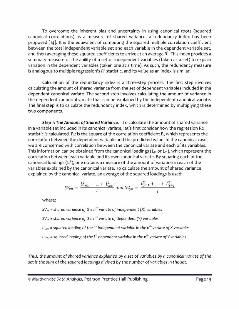
To overcome the inherent bias and uncertainty in using canonical roots (squared canonical correlations) as a measure of shared variance, a redundancy index has been proposed [14]. It is the equivalent of computing the squared multiple correlation coefficient between the total independent variable set and each variable in the dependent variable set, and then averaging these squared coefficients to arrive at an average R2. This index provides a summary measure of the ability of a set of independent variables (taken as a set) to explain variation in the dependent variables (taken one at a time). As such, the redundancy measure is analogous to multiple regression’s R2 statistic, and its value as an index is similar.

Calculation of the redundancy index is a three‐step process. The first step involves

calculating the amount of shared variance from the set of dependent variables included in the dependent canonical variate. The second step involves calculating the amount of variance in the dependent canonical variate that can be explained by the independent canonical variate. The final step is to calculate the redundancy index, which is determined by multiplying these two components.

Step 1: The Amount of Shared Variance. To calculate the amount of shared variance in a variable set included in its canonical variate, let’s first consider how the regression R2 statistic is calculated. R2 is the square of the correlation coefficient R, which represents the correlation between the dependent variable and the predicted value. In the canonical case, we are concerned with correlation between the canonical variate and each of its variables. This information can be obtained from the canonical loadings (LXi or LYi), which represent the correlation between each variable and its own canonical variate. By squaring each of the canonical loadings (Li2), one obtains a measure of the amount of variation in each of the variables explained by the canonical variate. To calculate the amount of shared variance explained by the canonical variate, an average of the squared loadings is used:

…

…

where:

SVxn = shared variance of the nth variate of independent (X) variables

SVyn = shared variance of the nth variate of dependent (Y) variables

L2XNI = squared loading of the ith independent variable in the nth variate of X variables

L2YNJ = squared loading of the jth dependent variable in the nth variate of Y variables

Thus, the amount of shared variance explained by a set of variables by a canonical variate of the set is the sum of the squared loadings divided by the number of variables in the set.


From our earlier example of credit card usage, the amount of shared variance for the first and the second canonical variates of independent variables can be calculated as:

0.82 0.75 0.35

3 0.45

0.30 0.69 0.79

3 0.40 Likewise, the amount of shared variance for the first and the second canonical variates of dependent variables is:

0.85 0.80 0.44

3 0.52

0.71 0.42 0.82

3 0.45 The first canonical variate explains 45 percent of the variance in consumer characteristics and the second canonical variate explains 40 percent. Together, the two canonical variates explain nearly 100 percent of the variance in consumer characteristics. For the credit card usage variables, the first canonical variate explains 52 percent of the variance and the second canonical variate explains 45 percent. When summing the two variates, almost 100 percent of variance in credit card usage is explained by the two canonical variates.

Step 2: The Amount of Explained Variance. The second step in calculating redundancy involves an estimate of the account of shared variance between the dependent and independent variates; namely, the canonical root. This is the squared correlation between the independent canonical variate and the dependent canonical variate. Recall that in our example the first pair of canonical variates had a canonical root of 85 percent and the second canonical root was 69 percent.

Step 3: The Redundancy Index. The redundancy index of a variate is then derived by

multiplying the two components (shared variance of the variate multiplied by the squared canonical correlation) to find the amount of shared variance explained by the opposite variate. To have a high redundancy index, one must have a high canonical correlation and a high degree of shared variance explained by its own variate. A high canonical correlation alone does not ensure a valuable canonical function. Redundancy indices are calculated for both the dependent and the independent variates, although in most instances the


researcher is concerned only with the variance extracted from the dependent variable set, which provides a much more realistic measure of the predictive ability of canonical relationships. The researcher should note that although the canonical correlation is the same for both variates in the canonical function, the redundancy index will most likely vary between the two variates, because each will have a differing amount of shared variance:

RI = SV * Rc2

The redundancy index of a canonical variate is the percentage of variance explained

by its own set of variables multiplied by the squared canonical correlation for the pair of variates. Thus, in our example, the redundancy indices for the independent variables explaining the dependent variables are:

RIx1: y = SVy1 x Rc12 = 0.52 x 0.85 ≈ 0.44 RIx2: y = SVy2 x Rc22 = 0.45 x 0.69 ≈ 0.31

The amounts of variance of the independent variables, explained by the dependent variables for the two functions, are:

RIy1: x = SVx1 x Rc12 = 0.45 x 0.85 ≈ 0.38 RIy2: y = SVx2 x Rc22 = 0.40 x 0.69 ≈ 0.28

That is, the first canonical variate for Consumer Characteristics explains 44 percent of the variance in Credit Card Usage and the second canonical variate explains 31 percent. Together they explain over 70 percent of the variance in the dependent variables. The first and the second canonical variates for Credit Card Usage explain 38 percent and 28 percent of the variance in Consumer Characteristics, respectively. Together they explain 66 percent of the variance in Consumer Characteristics.

What is the minimum acceptable redundancy index needed to justify the interpretation of canonical functions? Just as with canonical correlations, no generally accepted guidelines have been established. The researcher must judge each canonical function in light of its theoretical and practical significance to the research problem being investigated to determine whether the redundancy index is sufficient to justify interpretation. A test for the significance of the redundancy index has been developed [2], although it has not been widely utilized.


STAGE 5: INTERPRETING THE CANONICAL VARIATE If the canonical relationship is statistically significant and the magnitudes of the canonical root and the redundancy index are acceptable, the researcher still needs to make substantive interpretations of the results. Making these interpretations involves examining the canonical functions to determine the relative importance of each of the original variables in the canonical relationships. Three methods have been proposed: (1) canonical weights (standardized coefficients), (2) canonical loadings (structure correlations), and (3) canonical cross‐loadings.

CANONICAL WEIGHTS

The traditional approach to interpreting canonical functions involves examining the sign and the magnitude of the canonical weight assigned to each variable in its canonical variate. Variables with relatively larger weights contribute more to the variates, and vice versa. Similarly, variables whose weights have opposite signs exhibit an inverse relationship with each other, and variables with weights of the same sign exhibit a direct relationship. However, interpreting the relative importance or contribution of a variable by its canonical weight is subject to the same criticisms associated with the interpretation of beta weights in regression techniques. For example, a small weight may mean either that its corresponding variable is irrelevant in determining a relationship or that it has been partialed out of the relationship because of a high degree of multicollinearity. Another problem with the use of canonical weights is that these weights are subject to considerable instability (variability) from

Rules of Thumb 2

Choosing and Assessing Canonical Functions

• More than one canonical function can be derived, depending on the number of independent or dependent variables included

• The first function has the highest intercorrelation between the variates, the second function has the second-highest, and so forth

• Orthogonal rotation methods (e.g., Varimax) can increase the interpretability of canonical results, but it can also distort the fundamental logic of the method

• The canonical functions can be interpreted based on: • Their level of statistical significance • The size of the canonical correlation • The magnitude of the redundancy index

• The indices used varies based on the aims of the research problem and the guidelines within each discipline

• Canonical correlations can be judged by the same guidelines as factor loadings • Theoretical and practical significance are more important than statistical significance in determining the

minimum acceptable redundancy index


one sample to another. This instability occurs because the computational procedure for canonical analysis yields weights that maximize the canonical correlations for a particular sample of observed dependent and independent variable sets [10]. These problems suggest considerable caution in using canonical weights to interpret the results of a canonical analysis.

CANONICAL LOADINGS

Canonical loadings have been increasingly used as a basis for interpretation because of the deficiencies inherent in canonical weights. Canonical loadings, also called canonical structure correlations, measure the simple linear correlation between an original variable in the dependent or independent set and the set’s canonical variate. The canonical loading reflects the variance that the observed variable shares with the canonical variate and can be interpreted like a factor loading in assessing the relative contribution of each variable to each canonical function. The approach considers each independent canonical function separately and computes the within‐set variable‐to‐variate correlation. The larger the coefficient, the more important it is in deriving the canonical variate. Also, the criteria for determining the significance of canonical structure correlations are the same as with factor loadings (see Chapter 3).

Canonical loadings, like weights, may be subject to considerable variability from one sample to another. This variability suggests that loadings, and hence the relationships ascribed to them, may be sample‐specific, resulting from chance or extraneous factors [8]. Also, when using only canonical loadings for interpretation the risks increase that the application is closer to a univariate setting than to a multivariate one [13]. Although canonical loadings are considered relatively more valid than weights as a means of interpreting the nature of canonical relationships, the researcher must be cautious when using loadings for interpreting canonical relationships, particularly with regard to the external validity of the findings.

CANONICAL CROSS‐LOADINGS The computation of canonical cross‐loadings has been suggested as an alternative to canonical loadings [7]. This procedure involves correlating each of the variables directly with the other canonical variate, and vice versa. For example, each dependent variable would be correlated separately with the variate for the independent variables. Recall that conventional loadings correlate the variables with their respective variates after the two canonical variates (dependent and independent) are maximally correlated with each other. This may also seem similar to multiple regression, but it differs in that each independent variable, for example, is correlated with the dependent variate instead of a single dependent variable. Thus cross‐loadings provide a more direct measure of the dependent–independent


variable relationships by eliminating an intermediate step involved in conventional loadings. Some canonical analyses do not compute correlations between the variables and the variates. In such cases, the canonical weights are considered comparable but not equivalent for purposes of our discussion. The cross‐loadings can be expressed as:

Λxni: y = Rcn x Lxni Λynj: x = Rcn x Lxni

where

Λxni: y = cross‐loading of the ith independent variable in the nth variate X to the nth variate Y Λynj: x = cross‐loading of the jth dependent variable in the nth variate Y to the nth variate X Rcn = canonical correlation coefficient for the i

th canonical function Lxni = loading of the ith independent variable in the nth variate X Lxni = loading of the jth dependent variable in the nth variate Y

Thus, each canonical cross‐loading is equal to the product of canonical correlation coefficient for the nth canonical function and the canonical loading of the corresponding variable.

WHICH INTERPRETATION APPROACH TO USE

Several different methods for interpreting the nature of canonical relationships have been discussed. The question remains, however: Which method should the researcher use? Most often the researcher is constrained to the method(s) available in the statistical package being used. Canonical weights perform well in the multivariate setting because they adjust when the combination of the variable sets change [13]. However, they are valid only when collinearity is minimal. The canonical‐loadings approach is somewhat more representative than the use of weights, as was seen with factor analysis and discriminant analysis. Cross‐loadings and loadings are based on a linear relationship and thus have corresponding results. But cross‐loadings facilitate the transformation of a canonical model to a single latent construct which resembles Structural Equation Modeling [4]. Therefore, the cross‐loadings approach is preferred and whenever possible the loadings approach is recommended as the best alternative to the canonical cross‐loading method. Cross‐loadings are provided by many computer programs, but if the cross‐loadings are not available, the researcher is forced either to compute the cross‐loadings by hand or to rely on the interpretation of canonical loadings.


STAGE 6: VALIDATION AND DIAGNOSIS

As with other multivariate techniques, canonical correlation analysis should be subjected to validation methods to ensure that the results are specific not only to the sample data but can be generalized to the population. The most direct procedure is to create two subsamples of the data (if sample size allows) and perform the analysis on each subsample separately. Then the results can be compared for similarity of canonical functions, variate loadings, and the like. If marked differences are found, the researcher should consider additional investigation to ensure that the final results are representative of the population values, not solely those of a single sample. Another approach is to assess the sensitivity of the results to the removal of a dependent and/or independent variable. Because the canonical correlation procedure maximizes the correlation and does not optimize the interpretability, the canonical weights and loadings may vary substantially if one variable is removed from either variate. To ensure the stability of the canonical weights and loadings, the researcher should estimate multiple canonical correlations, each time removing a different independent or dependent variable. Although few diagnostic procedures have been developed specifically for canonical correlation analysis, the researcher should view the results within the limitations of the technique. Among the limitations that can have the greatest impact on the results and their interpretation are the following:

1. The canonical correlation reflects the variance shared by the linear composites of the sets of variables, not the variance extracted from the variables.

2. Canonical weights derived in computing canonical functions are subject to a great deal of instability.

3. Canonical weights are derived to maximize the correlation between linear composites, not the variance extracted.

4. The interpretation of the canonical variates may be difficult, because they are calculated to maximize the relationship, and aids for interpretation, such as rotation of variates in factor analysis, are limited.

Rules of Thumb 3

Interpreting and Validating Canonical Variates

• Canonical cross-loadings are preferred over canonical weights and canonical loadings when interpreting the results.

• If possible, the data should be split randomly into two subgroups, running canonical correlation analysis separately and comparing the results, in order to ensure the validity of the canonical solution.


5. It is difficult to identify meaningful relationships between the subsets of independent and dependent variables because precise statistics have not yet been developed to interpret canonical analysis, and we must rely on inadequate measures such as loadings or cross‐loadings [10].

These limitations are not meant to discourage the use of canonical correlation. Rather,

they are pointed out to enhance the effectiveness of canonical correlation as a research tool.

AN ILLUSTRATIVE EXAMPLE To illustrate the application of canonical correlation, we use variables drawn from the HBAT data‐base introduced in Chapter 1. Recall that the data consisted of a series of measures obtained on samples of HBAT customers. For this example, we chose the sample involving 200 customers (HBAT_200). The variables included ratings of HBAT on five measures of basic firm characteristics and respondents’ business relationship with HBAT (X1 to X5), 13 indicators reflecting perceptions of HBAT (X6 to X18), and five indicators of purchase outcome (X19 to X23), SPSS and Statit are used in the design and analysis of this example. Comparable results are obtained with other statistical programs available for commercial and academic use. The syntax and dataset of canonical correlation analysis is available on the text’s Web sites at www.pearsonglobaleditions. com/hair or www.mvstats.com.

This discussion of canonical correlation analysis follows the six‐stage process described earlier in the supplement. At each stage, the results illustrating the decisions in that stage are examined.

STAGE 1: OBJECTIVES OF CANONICAL CORRELATION ANALYSIS

In demonstrating the application of canonical correlation, 13 indicators of perceptions and 2 indicators of customers’ likelihood to do business with HBAT are used as input data. Both dependent and independent variables were assessed for meeting the basic assumptions underlying multivariate analyses. Among them, X14 and X18 are highly correlated with other variables. They are thus removed from the analysis due to their violation of multicollinearity. The HBAT ratings (X6 to X13 and X15 to X17) are designated as the set of independent variables. The set of dependent variables is defined as two variables—the likelihood of recommending HBAT and future purchases from HBAT (X20 and X21)

. The statistical problem involves identifying any relationships between the variates formed for customer perceptions of HBAT and the likelihood of doing business with HBAT in the future. This canonical model is illustrated in Figure 6.


STAGES 2 AND 3: DESIGNING A CANONICAL CORRELATION ANALYSIS AND TESTING THE ASSUMPTIONS The designation of the variables includes two metric‐dependent and 11 metric‐independent variables. The 11 variables resulted in an 18‐to‐1 ratio of observations to variables, exceeding the guideline of 10 observations per independent variable. The HBAT data set with 200 observations was used in this example. The sample size of 200 should not affect the estimates of sampling error markedly and thus should not impact the statistical significance of the results.

STAGE 4: DERIVING THE CANONICAL FUNCTIONS AND ASSESSING OVERALL FIT

The canonical correlation analysis was restricted to deriving two canonical functions because the dependent variable set contained only two indicators. To determine the number of canonical functions to include in the interpretation stage, the analysis focused on the level of statistical significance, the practical significance of the canonical correlation, and the redundancy indices for each variate.

STATISTICAL AND PRACTICAL SIGNIFICANCE

The first statistical significance test is for the canonical correlations of each of the two canonical functions. In this example, only the first canonical correlation is statistically significant (see Table 1). In addition to tests of each canonical function separately, multivariate tests of both functions were performed simultaneously. The test statistics employed included Wilks’ lambda, Pillai’s criterion, Hotelling’s trace, and Roy’s gcr. Table 1 also details the multivariate test statistics, which all indicate that the first canonical function, taken collectively, is statistically significant at the .01 level; the second canonical function fails to achieve significance level at the .05 level.

In addition to statistical significance, the canonical correlations show that only the first function is of sufficient size to be deemed practically significant. Because rotation is available only when there are at least two functions, rotation is not performed in this example.

REDUNDANCY ANALYSIS

A redundancy index is calculated for the independent and dependent variates of the first function in Table 2. As can be seen, the redundancy index for the dependent variate is substantial (.484). The independent variate, however, has a markedly lower redundancy index (.119), although in this case, because there is a clear delineation between dependent and independent variables, this


lower value is not unexpected or problematic. The low redundancy of the independent variate results from the relatively low shared variance in the independent variate (.204), not the canonical R2. From the redundancy analysis and the statistical significance tests, the first function should be accepted. The interested researcher should review Chapter 3, with attention to the discussion of scale development. Canonical correlation is in some ways a form of scale development, because the dependent and independent variates represent dimensions of the variable sets, similar to the scales developed with factor analysis. The primary difference is that these dimensions are developed to maximize the relationship between them, whereas factor analysis maximizes the explanation (shared variance) of the variable set.

STAGE 5: INTERPRETING THE CANONICAL VARIATES With the canonical relationship deemed statistically significant and the magnitude of the canonical root and the redundancy index acceptable, the researcher proceeds to making substantive interpretations of the results. Because the second function is considered statistically nonsignificant, it is excluded from further analysis and the interpretation phase. These interpretations involve examining the canonical function to determine the relative importance of each of the original variables in deriving the canonical relationships. The three methods for interpretation are (1) canonical weights (standardized coefficients), (2) canonical loadings (structure correlations), and (3) canonical cross‐loadings.

CANONICAL WEIGHTS

Table 4 contains the standardized canonical weights for each canonical variate of both the dependent and independent variables. As discussed earlier, the magnitude of the weights represents their relative contribution to the variate. The four variables with the highest canonical weights on the independent variate are X12 (Salesforce Image), X6 (Product Quality), X17 (Pricing Flexibility), and X11 (Product Line). The dependent variable order on the variate is X20 (Likelihood of Recommending), then X21 (Likelihood of Future Purchase). Recall that the weights obtained are typically unstable unless the collinearity among variables is minimal. In this example, X7 with X12 and X9 with X16 do share moderately high correlation (.788 and .741, respectively). Thus, the interpretation based on canonical weights is likely to be biased and therefore is not recommended in this example.


CANONICAL LOADINGS

Table 4 contains the canonical loadings for the dependent and independent variates for the first canonical function. The objective of maximizing the variates for the correlation between them results in variates “optimized” not for interpretation, but rather for prediction. This makes identification of relationships more difficult. In the first dependent variate, both variables have loadings exceeding .80, resulting in the high shared variance (.824). This indicates a high degree of intercorrelation among the two variables and suggests that both or either measures are representative of customer intentions to do business with HBAT.

The first independent variate has a quite different pattern, with loadings ranging from .036 to .661, with one independent variable (X13) even having a negative loading, although it is rather small and not of substantive interest. The four variables with the highest loadings on the independent variate are X11 (Product Line), X6 (Product Quality), X9 (Complaint Resolution), and X16 (Ordering and Billing). This variate partly corresponds to the dimensions extracted in factor analysis (see Chapter 3), but it would not be expected to fully match because the variates in canonical correlation are extracted only to maximize predictive objectives. As such, it should correspond more closely to the results from other dependence techniques.

There is a close correspondence to the multiple regression results summarized in

Chapter 4. Two of these variables (X6 and X11) were included in the stepwise regression analysis in which X21 (one of the two variables in the dependent variate) was the dependent variable. Thus, the first canonical function closely corresponds to the multiple regression results, with the independent variate representing the set of variables best predicting the two dependent measures. The researcher should also perform a sensitivity analysis of the independent variate to see whether the loadings change when an independent variable is deleted (see stage 6).

CANONICAL CROSS‐LOADINGS

Table 4 also includes the cross‐loadings for the two canonical functions. In studying the first canonical function, we see that both dependent variables (X20 and X21) exhibit high correlations with the independent canonical variate ‐ .717 and .674, respectively. This reflects the high shared variance between these two variables. By squaring these terms, we find the percentage of the variance for each of the variables explained by function 1. The results show that 51.4 percent of the variance in X20 and 45.4 percent of the variance in X21 is explained by function 1. Looking at the independent variables’ cross‐loadings, we see that variables X11 and X6 have the highest correlations with the dependent canonical variate ‐ .506 and .476, respectively. From this information, approximately 25.6 percent of the variance in X11 and 22.7 percent of variance in X6 are explained by the dependent variate (the 25.6% is obtained by squaring the


correlation coefficient, .506).

The final issue of interpretation is examining the signs of the cross‐loadings. All independent variables except X13 (Competitive Pricing) have a positive, direct relationship. The four highest cross‐loadings of the independent variate correspond to the variables with the highest canonical loadings as well. Thus all the relationships are positive except for one inverse relationship (X13).

STAGE 6: VALIDATION AND DIAGNOSIS

The last stage should involve a validation of the canonical correlation analyses through one of several procedures. Among the available approaches would be (1) splitting the sample into estimation and validation samples or (2) sensitivity analysis of the independent variables set. Table 5 contains the results of a sensitivity analysis in which the canonical loadings are examined for stability when individual independent variables are deleted from the analysis. As seen, the canonical loadings in our example are remarkably stable and consistent in each of the three cases where an independent variable (X6, X7, or X8) is deleted. The overall canonical correlations also remain stable. But the researcher examining the canonical weights (not presented in the table) would find widely varying results, depending on which variable was deleted. This reinforces the procedure of using the canonical loadings and cross‐loadings for interpretation purposes.

A MANAGERIAL OVERVIEW OF THE RESULTS

The canonical correlation analysis addresses two primary objectives: (1) identification of dimensions among the dependent and independent variable sets and (2) maximization of the relationship between the dimensions. From a managerial perspective, this provides the researcher with insights into the structure of the different variable sets as they relate to a dependence relationship. First, the results indicate that only a single relationship exists, supported by the lack of statistical significance and low practical significance of the second canonical function. In examining this relationship, we first see that the two dependent variables are quite closely related and create a well‐defined dimension for representing the outcomes of HBAT’s efforts. Second, this outcome dimension is fairly well predicted by the set of independent variables when acting as a set. The redundancy value of .484 would be an acceptable R2 for a comparable multiple regression. When interpreting the independent variate, we see that three variables, X11 (Product Line), X6 (Product Quality), and X9 (Complaint Resolution) provide the substantive contributions and thus are the key predictors of the outcome dimension. These should be the focal points in the development of any strategy directed toward impacting the outcomes of HBAT’s future actions.


SUMMARY

The concept of canonical correlation analysis and a decision‐making procedure for this technique have been introduced in this supplement. Basic guidelines for assessing the results are also included and an example of the application of canonical correlation analysis with the HBAT data set is presented to further clarify the methodological concepts.

Describe canonical correlation analysis and under‐stand its purpose. Canonical correlation analysis is a useful and powerful technique for exploring the relation‐ships among multiple dependent and independent variables. The technique is primarily descriptive, although it can be used for predictive purposes. Results obtained from a canonical analysis should suggest answers to questions concerning the number of ways in which the two sets of multiple variables are related, the strengths of the relationships, and the nature of the relationships defined. Canonical analysis enables the researcher to combine into a composite measure what otherwise might be an unmanageably large number of bivariate correlations between sets of variables. It is useful for identifying overall relationships between multiple independent and dependent variables, particularly when the researcher has little a priori knowledge about relationships among the sets of variables. Essentially, the researcher can apply canonical correlation analysis to a set of variables, select those variables (both independent and dependent) that appear to be significantly related, and run subsequent canonical correlations with the more significant variables remaining or perform individual regressions with these variables.

State the similarities and differences between multiple regression, discriminant analysis, factor analysis, and canonical correlation. Canonical correlation analysis is the most general form of the multivariate statistical techniques. It can have multiple dependent variables that can be metric or nonmetric. It is similar to multiple regression in that the goal of canonical correlation analysis is to quantify the strength of the relation‐ships between independent variables and dependent variable(s). It also resembles discriminant analysis in its ability to determine independent dimensions. Like factor analysis, canonical correlation analysis can create an optimized structure for a set of variables. However, canonical correlation analysis is unique in that it can integrate more than one dependent variable, which is not possible with multiple regression and discriminant analysis. Factor analysis gives details about the linear relationship between the measured variables and latent variables, but canonical correlation focuses more on the linear relationship between a pair of canonical variates.

Summarize the conditions that must be met for application of canonical correlation analysis. Strong theoretical support is needed for selecting and grouping variables, as well as determining the research objectives. However, it is of little importance to strictly define the latent variables into independent and dependent canonical variates, because the technique does not differentiate between the two sets when weighting both variates to


maximize the correlation. Even though canonical correlation analysis is relatively less demanding in meeting the underlying statistical assumptions, interpretability is improved if the assumptions are satisfied. These include linearly, normality, homoscedasticity, and multicollinearity. Missing data and outliers should also be avoided.

Define and compare canonical root measures and the redundancy index. A canonical root is the squared canonical correlation coefficient. It indicates the amount of shared variance between the two respective optimally weighted canonical variates. It tells the researcher the proportion of variance explained in the canonical variates but it does not differentiate how much variance is explained in each of the two sets of variables themselves. The canonical root is the same for both variates in the canonical function.

The redundancy index is the amount of variance in a canonical variate explained by the opposite canonical variate in the canonical function. It reflects how well the independent canonical variate predicts values of the dependent variables. The redundancy index is similar to a regression R2—high redundancy means high ability to predict. It suggests the ability of a set of independent variables to explain variation in the dependent variables, or vice versa. Thus, the redundancy indices are different for dependent and independent variates.

Compare the advantages and disadvantages of the three methods for interpreting the nature of canonical functions. The canonical function can be interpreted by the sign and the magnitude of the canonical weights assigned to each variable in its respective canonical variate. Variables with larger weights contribute more to the variates, and vice versa. Because canonical weights are derived to maximize the canonical correlations, they are subject to considerable instability from one sample to another. Also, weights may be distorted due to multicollinearity. Therefore, considerable caution is necessary if interpretation is based on canonical weights.

Canonical loadings measure the correlation between the original observed variables and its canonical variate. They can be interpreted like factor loadings. Variables with larger loadings are more important in deriving the canonical variate. Whereas weights are more suitable for prediction, loadings are better at explaining underlying constructs. Canonical loadings are considered more valid and stable than weights.

Canonical cross‐loadings measure the correlation between the original observed variables and their opposite variate (i.e., independent variables correlate to the dependent variate, dependent variables correlate to the independent variate). They offer more direct interpreta‐tions by eliminating an intermediate step of conventional loadings. However, computation of cross‐loadings is not as widely available as canonical loadings and weights in statistical programs.


Questions

1. Under what circumstances would you select canonical correlation analysis over multiple regression as the appropriate statistical technique?

2. What three criteria should you use in deciding which canonical functions should be interpreted? Explain the role of each.

3. How would you interpret a canonical correlation analysis? 4. What is the relationship among the canonical root, the redundancy index, and multiple

regression’s R2? 5. What are the limitations associated with canonical correlation analysis? 6. Why has canonical correlation analysis been used much less frequently than other

multivariate techniques?

Suggested Readings

A list of suggested readings illustrating issues and applications of canonical correlation in general is available on the Web at www.pearsonglobaleditions.com/hair or www.mvstats.com.

References

1. Alpert, Mark I., and Robert A. Peterson. 1972. On the Interpretation of Canonical Analysis. Journal of Marketing Research 9 (May): 187.

2. Alpert, Mark I., Robert A. Peterson, and Warren S. Martin. 1975. Testing the Significance of Canonical Correlations. Proceedings, American Marketing Association 37: 10. 117–19.

3. Aksin, Zeynep O., and Andrea Masini. 2008. Effective Strategies for Internal Outsourcing and Offshoring of 11. Business Services: An Empirical Investigation. Journal of Operations Management 26: 239–56. 12.

4. Bagozzi, R. P., C. Fornell, and D. F. Larcker. 1981. Canonical Correlation Analysis as a Special Case of a Structural Relations Model. Multivariate Behavioral 13. Research 16(4): 437–54.

5. Bartlett, M. S. 1941. The Statistical Significance of 14. Canonical Correlations. Biometrika 32: 29.

6. Van der Burg, Eeke, Jan de Leeuw, and Garmt Dijksterhuis. 1994. OVERALS: Nonlinear Canonical Correlation with K 15. Sets of Variables. Computational Statistics & Data Analysis 18: 141–63. 16.

7. Dillon, W. R., and M. Goldstein. 1984. Multivariate Analysis: Methods and Applications. New York: Wiley.


8. Green, P. E. 1978. Analyzing Multivari ate Data. Hinsdale, IL: Holt, Rinehart, & Winston. 9. Green, P. E., and J. Douglas Carroll. 1978. Mathematical Tools for Applied Multivariate Analysis. New York: Academic Press.

10. Lambert, Z., and R. Durand. 1975. Some Precautions in Using Canonical Analysis. Journal of Marketing Research 12 (November): 468–75.

11. Levine, Mark S. 1977. Canonical Analysis and Factor Comparison. Newbury Park, CA: Sage. 12. Lukas, Bryan A., and O. C. Ferrell. 2000. The Effect of Market Orientation on Product Innovation. Journal of Academy of Marketing Science 28: 239–47.

13. Rencher, Alvin C. 2002. Methods of Multivariate Analysis, 2d ed. New York: John Wiley and Sons.

14. Stewart, Douglas, and William Love. 1968. A General Canonical Correlation Index. Psychological Bulletin 70: 160–63.

15. Thompson, Bruce. 1984. Canonical Correlation Analysis: Uses and Interpretation. Newbury Park, CA: Sage.

16. Thompson, Bruce. 1991. A Primer on the Logic and Use of Canonical Correlation Analysis. Measurement and Evaluation in Counseling and Development 24: 80–95.

© Multiva

Figure Variate

F

F

Figure 2Credit C

ariate Data A

1 Relations in the Ca

Family size

Family Income

Credit History

2 CanoniCard Usage

Analysis, Pea

nship of Vanonical Fu

ConCha

cal Relatioe

arson Prent

Variables aunction

nsumer aracteristics

onship be

tice Hall Pub

and Canon

etween Co

blishing

nical Loadi

Credit Card Usage

onsumer C

ings with

Num

AveSpe

OutsBala

Characteris

Pag

the Canon

mber of Cards

rage Monthly nding

standing ance

stics and t

ge 35

nical

their

© Multiva

Figure 3the Hyp

ariate Data A

3 Canonicapothetical

Analysis, Pea

al LoadingExample

arson Prent

gs and Corr

tice Hall Pub

relations fo

blishing

or the Twoo Canonica

Pag

al Function

ge 36

ns of


Stage 1

Stage 2

Stage 3

Research ProblemSelecting and justifying variable sets

Determining research objectives

Research DesignObtaining appropriate sample size

Variables and their conceptual linkageHandling missing data and outliers

Assumptions of AnalysisStatistical consideration of

linearity, normality, homoscedasticity

and multicollinearity

No

Stage 4

Figure 4 Stages 1‐3 in the Canonical Correlation Analysis Decision Diagram


Stage 4

Stage 5

Stage 6

Stage 3

Deriving and Assessing Canonical FunctionsDetermining the number of function derived

Assessing the function(s) •Is it statistically significant?

•Is the magnitude of the relationship acceptable?•Is the size of redundancy index satisfactory?

Interpreting Canonical VariatesDetermining which method for interpreting

•Canonical Weights•Canonical Loadings

•Canonical Cross-Loadings

Validation and DiagnosisSplit samples into two groups

Separate analysis for subsamplesCompare for similarity of canonical indexes

Figure 5 Stages 4‐6 in the Canonical Correlation Analysis Decision Diagram


X21 Likelihood of Future Purchase from HBAT

X20 Likelihood of Recommending HBAT

X6 Product Quality

X7 E-commerce Activities/Website

X8 Technical Support

X9 Complaint Resolution

X10 Advertising

X11 Product Line

X12 Salesforce Image

X13 Competitive Pricing

X15 New Products

X16 Ordering and Billing

X17 Price Flexibility

Consumer Perceptions

Likelihood for Future Business

Figure 6 Canonical Correlation of Likelihood for Future Business with HBAT and Customers’ Perception about HBAT


Table 1 Canonical correlation analysis relating perceptions of HBAT to likelihood to do business with HBAT

Measures of overall Model Fit for Canonical Correlation Analysis Canonical Function

Canonical Correlation

Canonical R2 F Statistics Probability

1 .765 .585 9.956 .000 2 .203 .041 .807 .622

Multivariate Tests of Significance Statistic Value Approximate F

Statistic Probability

Wilks’ lambda .398 9.956 .000 Pillai’s trace .626 7.793 .000 Hotelling’s trace 1.454 12.291 .000 Roy’s gcr .585


Table 2 Calculation of the Redundancy Indices for the First Canonical Function

Variate/Variables Canonical

Loading Canonical Loading Squared

Average Loading Squared

Canonical R2

Redundancy Index

Dependent Variables

X20 Likelihood of recommending HBAT

.938 .880

X21 Likelihood of future purchases from HBAT

.881 .776

Dependent Variate 1.656 ≅.827 .585 .484

Independent Variables

X6 Product quality .622 .387 X7 E-commerce .393 .154 X8 Technical support .328 .108 X9 Complaint resolution .605 .366 X10 Advertising .336 .113 X11 Product line .661 .437 X12 Salesforce image .524 .275 X13 Competitive pricing -.291 .085 X15 New products .150 .023 X16 Ordering and billing .540 .292 X17 Pricing flexibility .036 .001

Independent Variate 2.239 ≅.204 .585 ≅.119


Table 3 Redundancy Analysis of Dependent and Independent Variates for Both Canonical Functions

Standardized Variance of the Dependent Variables Explained by

Their Own Canonical Variate (Shared Variance)

The Opposite Canonical Variate (Redundancy)

Canonical

Function

Percentage Cumulative

Percentage

Canonical

R2


Percentage

1 .827 .827 .585 .484 .484

Standardized Variance of the Independent Variables Explained by

Their Own Canonical Variate (Shared Variance)

The Opposite Canonical Variate (Redundancy)

Canonical

Function


Percentage

Canonical

R2


Percentage

1 .204 .204 .585 .119 .119


Table 4 Canonical Weights, Loadings and Cross‐Loadings for the Canonical Function

Canonical Weights Canonical Loadings

Canonical Cross-Loadings

Independent Variables X6 Product quality .631 .622 .476 X7 E-commerce -.139 .393 .301 X8 Technical support .161 .328 .251 X9 Complaint resolution .026 .605 .463 X10 Advertising -.120 .336 .257 X11 Product line .416 .661 .506 X12 Salesforce image .657 .524 .401 X13 Competitive pricing -.087 -.291 -.222 X15 New products -.013 .150 .114 X16 Ordering and billing -.043 .540 .413 X17 Pricing flexibility .421 .036 .028 Dependent Variables X20 Likelihood of recommending HBAT

.632 .938 .717


.462 .881 .674


Table 5 Sensitivity Analysis of the Canonical Correlation Results to Removal of an Independent Variable

Results after Deletion of Complete

Variate X6 X7 X8

Canonical correlation (R) .765 .668 .762 .756 Canonical root (R2) .585 .447 .581 .571 INDEPENDENT VARIATE Canonical loadings X6 Product quality .622 omitted .624 .630 X7 E-commerce .393 .452 omitted .398 X8 Technical support .328 .376 .329 omitted X9 Complaint resolution .605 .692 .607 .613 X10 Advertising .336 .384 .337 .340 X11 Product line .661 .756 .663 .670 X12 Salesforce image .524 .601 .526 .530 X13 Competitive pricing -.291 -.331 -.291 -.295 X15 New products .150 .173 .151 .151 X16 Ordering and billing .540 .621 .543 .546 X17 Pricing flexibility .036 .043 .037 .036 Shared variance .204 .243 .210 .219 Redundancy .120 .109 .122 .125 DEPENDENT VARIATE Canonical loadings X20 Likelihood of recommending HBAT

.938 .944 .941 .935


.881 .872 .876 .884

Shared variance .827 .825 .826 .828 Redundancy .484 .369 .480 .473

Canonical Correlation: A Supplement to Multivariate - MVSTATS

Documents

Transcript of Canonical Correlation: A Supplement to Multivariate - MVSTATS