Bastien Mussard · A short presentation (1) What I do : Quantum Mechanics I Wavefunction theories...

Developments in Electronic Structure Theory.

Bastien Mussard

Laboratoire de Chimie TheoriqueInstitut du Calcul et de la Simulation

Sorbonne Universites, Universite Pierre et Marie Curie

[email protected]/pagesperso/mussard/

www.lct.jussieu.fr/pagesperso/mussard/

A short presentation

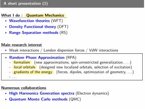
A short presentation (1)

What I do : Quantum MechanicsI Wavefunction theories (WFT)

I Density Functional theory (DFT)

I Range Separation methods (RS)

Main research interestI Weak interactions / London dispersion forces / VdW interactions

I Random Phase Approximation (RPA)- formalism (new approximations, spin-unrestricted generalization, . . .)- local orbitals (designed new localized orbitals, selection of excitation)- gradients of the energy (forces, dipoles, optimization of geometry, . . .)- . . .

Numerous collaborationsI High Harmonics Generation spectra (Electron dynamics)

I Quantum Monte Carlo methods (QMC)

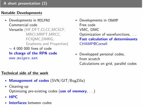
A short presentation (2)

Notable Developments

I Developments in MOLPRO

Commercial codeVersatile (HF,DFT,CI,CC,MCSCF,

MRCI,MRPT,MRCC,FCIQMC,DMRG,Gradients and Properties)

∼ 4 000 000 lines of codeIn charge of the RPA codewww.molpro.net

I Developments in CHAMP

Free codeVMC, DMCOptimization of wavefunctions, . . .Fast calculation of determinantsCHAMP@Cornell

I Developped personal codes,from scratchCalculations on grid, parallel codes

Technical side of the work

I Management of codes (SVN/GIT/BugZilla)

I Cleaning-upOptimizing pre-existing codes (use of memory, . . .)

I HPC

I Interfaces between codes

www.molpro.net

http://pages.physics.cornell.edu/~cyrus/champ.html

Context of my main research interest

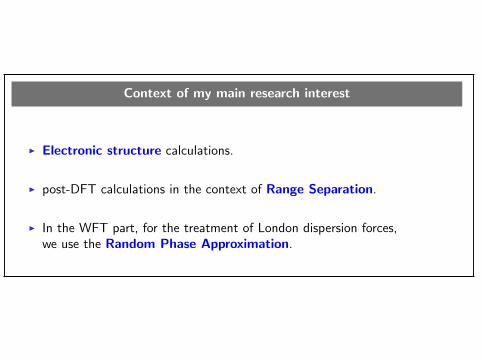
I Electronic structure calculations.

I post-DFT calculations in the context of Range Separation.

I In the WFT part, for the treatment of London dispersion forces,we use the Random Phase Approximation.

Range Separation : Motivation [Savin, Rec.dev. (1996)]

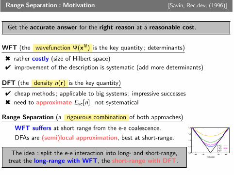
Get the accurate answer for the right reason at a reasonable cost.

WFT (the wavefunction Ψ(xN) is the key quantity ; determinants)

6 rather costly (size of Hilbert space)

4 improvement of the description is systematic (add more determinants)

DFT (the density n(r) is the key quantity)

4 cheap methods ; applicable to big systems ; impressive successes

6 need to approximate Exc [n] ; not systematical

Range Separation (a rigourous combination of both approaches)

WFT suffers at short range from the e-e coalescence.

DFAs are (semi)local approximation, best at short-range.

The idea : split the e-e interaction into long- and short-range,treat the long-range with WFT, the short-range with DFT.

1.0

1.1

1.2

1.3

1.4

−40 −20 20 40

θ (degree)

L = 1L = 2L = 3L = 4L = ∞

Range Separation : Realisation [Savin, Rec.dev. (1996)]

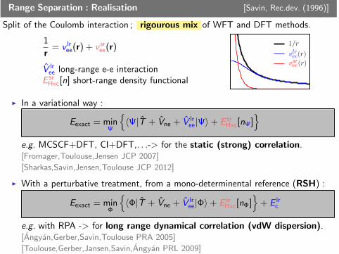
Split of the Coulomb interaction ; rigourous mix of WFT and DFT methods.

1

r= v lr

ee(r) + v sree(r)

V lree long-range e-e interaction

E srHxc[n] short-range density functional

1/r

vlree(r)

vsree(r)

I In a variational way :

Eexact = minΨ

{〈Ψ|T + Vne + V lr

ee|Ψ〉+ E srHxc[nΨ]

}e.g. MCSCF+DFT, CI+DFT,. . .-> for the static (strong) correlation.[Fromager,Toulouse,Jensen JCP 2007]

[Sharkas,Savin,Jensen,Toulouse JCP 2012]

I With a perturbative treatment, from a mono-determinental reference (RSH) :

Eexact = minΦ

{〈Φ|T + Vne + V lr

ee|Φ〉+ E srHxc[nΦ]

}+ E lr

c

e.g. with RPA -> for long range dynamical correlation (vdW dispersion).[Angyan,Gerber,Savin,Toulouse PRA 2005]

[Toulouse,Gerber,Jansen,Savin,Angyan PRL 2009]

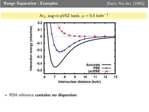
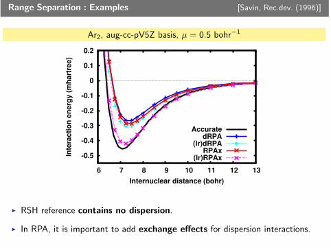
Range Separation : Examples [Savin, Rec.dev. (1996)]

Ar2, aug-cc-pV5Z basis, µ = 0.5 bohr−1

-0.5

-0.4

-0.3

-0.2

-0.1

0

0.1

0.2

6 7 8 9 10 11 12 13

Inte

rac

tio

n e

ne

rgy

(m

ha

rtre

e)

Internuclear distance (bohr)

AccuratePBE

(sr)PBE

I RSH reference contains no dispersion.

I In RPA, it is important to add exchange effects for dispersion interactions.

Range Separation : Examples [Savin, Rec.dev. (1996)]

Ar2, aug-cc-pV5Z basis, µ = 0.5 bohr−1

-0.5

-0.4

-0.3

-0.2

-0.1

0

0.1

0.2

6 7 8 9 10 11 12 13

Inte

rac

tio

n e

ne

rgy

(m

ha

rtre

e)

Internuclear distance (bohr)

AccuratedRPA

(lr)dRPARPAx

(lr)RPAx

I RSH reference contains no dispersion.

I In RPA, it is important to add exchange effects for dispersion interactions.

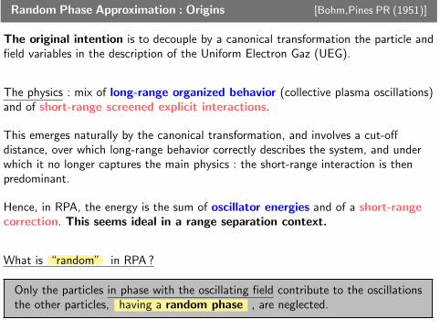
Random Phase Approximation : Origins [Bohm,Pines PR (1951)]

The original intention is to decouple by a canonical transformation the particle andfield variables in the description of the Uniform Electron Gaz (UEG).

The physics : mix of long-range organized behavior (collective plasma oscillations)and of short-range screened explicit interactions.

This emerges naturally by the canonical transformation, and involves a cut-offdistance, over which long-range behavior correctly describes the system, and underwhich it no longer captures the main physics : the short-range interaction is thenpredominant.

Hence, in RPA, the energy is the sum of oscillator energies and of a short-rangecorrection. This seems ideal in a range separation context.

What is “random” in RPA ?

Only the particles in phase with the oscillating field contribute to the oscillationsthe other particles, having a random phase , are neglected.

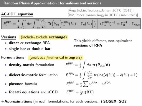
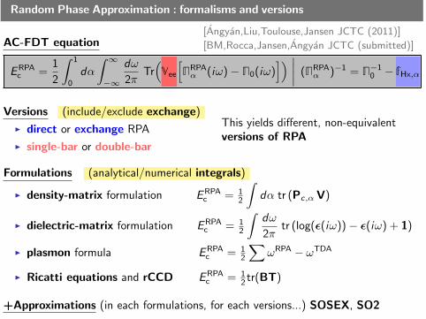
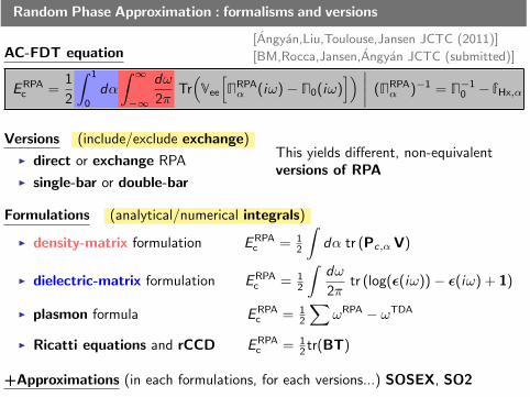
Random Phase Approximation : formalisms and versions

[Angyan,Liu,Toulouse,Jansen JCTC (2011)]

[BM,Rocca,Jansen,Angyan JCTC (submitted)]AC-FDT equation

ERPAc =

1

2

∫ 1

0

dα

∫ ∞−∞

dω

2πTr(Vee

[�RPAα (iω)− �0(iω)

]) ∣∣∣∣ (�RPAα )−1 = �−1

0 − fHx,α

Versions (include/exclude exchange)

I direct or exchange RPA

I single-bar or double-bar

This yields different, non-equivalentversions of RPA

Formulations (analytical/numerical integrals)

I density-matrix formulation ERPAc = 1

2

∫dα tr (Pc,α V)

I dielectric-matrix formulation ERPAc = 1

2

∫dω

2πtr (log(ε(iω))− ε(iω) + 1)

I plasmon formula ERPAc = 1

2

∑ωRPA − ωTDA

I Ricatti equations and rCCD ERPAc = 1

2 tr(BT)

+Approximations (in each formulations, for each versions...) SOSEX, SO2

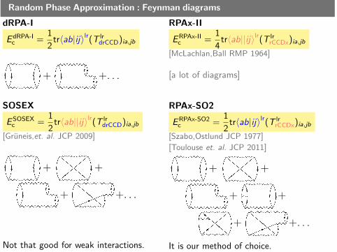
Random Phase Approximation : Feynman diagrams

dRPA-I

E dRPA-Ic =

1

2tr〈ab|ij〉lr(T lr

drCCD)ia,jb

+ +. . .

SOSEX

ESOSEXc =

1

2tr〈ab||ij〉lr(T lr

drCCD)ia,jb

[Gruneis,et. al. JCP 2009]

+ +

+ +. . .

Not that good for weak interactions.

RPAx-II

ERPAx-IIc =

1

4tr〈ab||ij〉lr(T lr

rCCDx)ia,jb

[McLachlan,Ball RMP 1964]

[a lot of diagrams]

RPAx-SO2

ERPAx-SO2c =

1

2tr〈ab|ij〉lr(T lr

rCCDx)ia,jb

[Szabo,Ostlund JCP 1977]

[Toulouse et. al. JCP 2011]

+ +

+ +

+ +. . .

It is our method of choice.

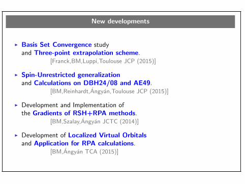
New developments

I Basis Set Convergence studyand Three-point extrapolation scheme.

[Franck,BM,Luppi,Toulouse JCP (2015)]

I Spin-Unrestricted generalizationand Calculations on DBH24/08 and AE49.

[BM,Reinhardt,Angyan,Toulouse JCP (2015)]

I Development and Implementation ofthe Gradients of RSH+RPA methods.

[BM,Szalay,Angyan JCTC (2014)]

I Development of Localized Virtual Orbitalsand Application for RPA calculations.

[BM,Angyan TCA (2015)]

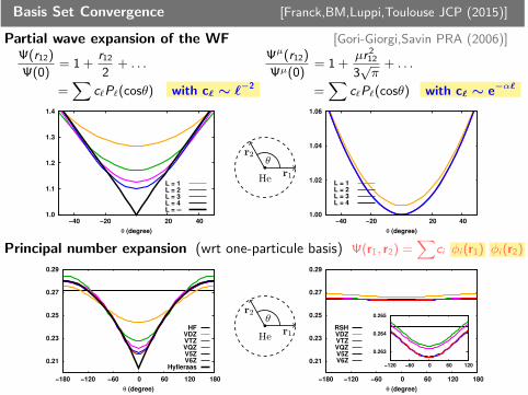
Basis Set Convergence [Franck,BM,Luppi,Toulouse JCP (2015)]

Partial wave expansion of the WF [Gori-Giorgi,Savin PRA (2006)]Ψ(r12)

Ψ(0)= 1 +

r12

2+ . . .

=∑

c`P`(cosθ) with c` ∼ `−2

Ψµ(r12)

Ψµ(0)= 1 +

µr 212

3√π

+ . . .

=∑

c`P`(cosθ) with c` ∼ e−α`

1.0

1.1

1.2

1.3

1.4

−40 −20 20 40

θ (degree)

L = 1L = 2L = 3L = 4L = ∞

Her1

r2θ

1.00

1.02

1.04

1.06

−40 −20 20 40

θ (degree)

L = 1L = 2L = 3L = 4

Principal number expansion (wrt one-particule basis) Ψ(r1, r2) =∑

ci φi (r1) φi (r2)

0.21

0.23

0.25

0.27

0.29

−180 −120 −60 0 60 120 180

θ (degree)

HFVDZVTZVQZV5ZV6Z

Hylleraas

Her1

r2θ

0.21

0.23

0.25

0.27

0.29

−180 −120 −60 0 60 120 180

θ (degree)

RSHVDZVTZVQZV5ZV6Z

0.263

0.264

0.265

−120 −60 0 60 120

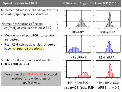
Spin-Unrestricted RPA [BM,Reinhardt,Angyan,Toulouse JCP (2015)]

Implemented most of the variants with anospinflip/spinflip block structure.

Normal distributions of errors(kcal/mol) of calculations on AE49.

⟩I Mean errors of post-RSH calculation

are better.

I Post-RSH calculations dist. of errorshave sharper distributions .

Similar results were obtained on theDBH24/08 dataset.

We argue that RPAx-SO2 is a goodmethod for a wide range of

applications.

0

0.04

0.08

0.12

-40 -20 0 20

HF+MP2

0

0.04

0.08

0.12

-40 -20 0 20

RSH+MP2

0

0.04

0.08

0.12

-40 -20 0 20

HF+dRPA-I

0

0.04

0.08

0.12

-40 -20 0 20

RSH+dRPA-I

0

0.04

0.08

0.12

-40 -20 0 20

HF+RPAx-SO2

0

0.04

0.08

0.12

-40 -20 0 20

RSH+RPAx-SO2

>cc-pVQZ (post-RSH : srPBE, µ = 0.5)

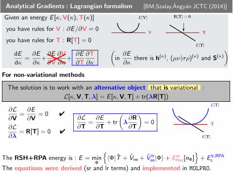
Analytical Gradients : Lagrangian formalism [BM,Szalay,Angyan JCTC (2014)]

Given an energy E [κ,V(κ),T(κ)]

you have rules for V : ∂E/∂V = 0

you have rules for T : R[T] = 0

energie

energie

(c)(b)(a)

parametreparametreparametre

energie

lagrangien

T TV

R[T] = 0E[V]

E[T] E[T]

L[T]

energie

energie

(c)(b)(a)


energie

lagrangien

T TV

R[T] = 0E[V]

E[T] E[T]

L[T]

dE

dκ=∂E

∂κ+∂E

∂V

∂V

∂κ×+∂E

∂T

∂T

∂κ

(in∂E

∂κthere is h(κ), (µν|σρ)(κ) and S(κ)

)For non-variational methods

The solution is to work with an alternative object that is variational :

L[κ,V,T,λ] = E [κ,V,T] + tr(λR[T])

∂L∂V

=∂E

∂V= 0 4

∂L∂λ

= R[T] = 0 4

∂L∂T

=∂E

∂T+ tr

(λ∂R

∂T

)= 0

energie

energie

(c)(b)(a)


energie

lagrangien

T TV

R[T] = 0E[V]

E[T] E[T]

L[T]

The RSH+RPA energy is : E = minΦ

{〈Φ|T + Vne + V lr

ee|Φ〉+ E srHxc[nΦ]

}+ E lr,RPA

c

The equations were derived (sr and lr terms) and implemented in MOLPRO.

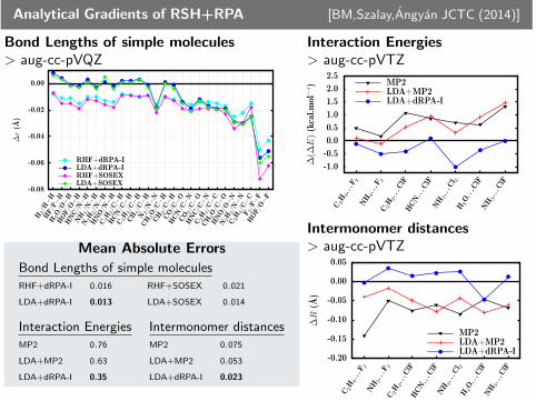
Analytical Gradients of RSH+RPA [BM,Szalay,Angyan JCTC (2014)]

Bond Lengths of simple molecules> aug-cc-pVQZ

-0.08

-0.06

-0.04

-0.02

0.00

H2/H

−HHF/F−H

H2O/O

−HHOF/O

−HHNC/N

−HNH3/N

−HN2H2/N

−HHNO/N

−HC 2

H2/C−H

HCN/C−H

C 2H4/C−H

CH4/C−H

N2/N

−NCH2O/C−H

CH2/C−H

CO/C−O

HCN/C−N

CO2/C−O

HNC/C−N

C 2H2/C−C

CH2O/C−O

HNO/O

−NN2H2/N

−NC 2

H4/C−C

F 2/F−F

HOF/O

−F

∆r

(Å)

RHF+dRPA-ILDA+dRPA-IRHF+SOSEXLDA+SOSEX

Mean Absolute Errors

Bond Lengths of simple moleculesRHF+dRPA-I 0.016 RHF+SOSEX 0.021

LDA+dRPA-I 0.013 LDA+SOSEX 0.014

Interaction Energies Intermonomer distancesMP2 0.76 MP2 0.075

LDA+MP2 0.63 LDA+MP2 0.053

LDA+dRPA-I 0.35 LDA+dRPA-I 0.023

Interaction Energies> aug-cc-pVTZ

-1.0

-0.5

0.0

0.5

1.0

1.5

2.0

2.5

C2H4. .

. F2

NH3. .

. F2

C2H2. .

. ClF

HCN. .

. ClF

NH3. .

. Cl 2

H2O. .

. ClF

NH3. .

. ClF

∆(∆

E)

(kca

l.m

ol−1) MP2

LDA+MP2LDA+dRPA-I

Intermonomer distances> aug-cc-pVTZ

-0.20

-0.15

-0.10

-0.05

0.00

0.05

C2H4. .

. F2

NH3. .

. F2

C2H2. .

. ClF

HCN. .

. ClF

NH3. .

. Cl 2

H2O. .

. ClF

NH3. .

. ClF

∆R

(Å)

MP2LDA+MP2LDA+dRPA-I

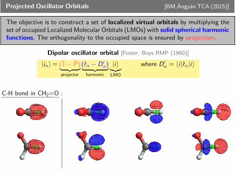
Projected Oscillator Orbitals [BM,Angyan TCA (2015)]

The objective is to construct a set of localized virtual orbitals by multiplying theset of occupied Localized Molecular Orbitals (LMOs) with solid spherical harmonicfunctions. The orthogonality to the occupied space is ensured by projection.

Dipolar oscillator orbital [Foster, Boys RMP (1960)]

|iα〉= (1− P)︸︷︷︸projector

(rα − D iα)︸︷︷︸

harmonic

|i〉︸︷︷︸LMO

where D iα = 〈i |rα|i〉

C-H bond in CH2=O :∣∣∣∣∣∣∣∣∣∣∣∣∣∣∣∣∣∣

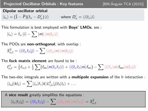
Projected Oscillator Orbitals : Key features [BM,Angyan TCA (2015)]

Dipolar oscillator orbital

|iα〉= (1− P)(rα − D iα) |i〉 where D i

α = 〈i |rα|i〉

This formulation is best employed with Boys’ LMOs, see :

|iα〉= rα |i〉−∑|m〉〈m|rα|i〉

The POOs are non-orthogonal, with overlap :

S ijαβ = 〈i |rαrβ |j〉 −

∑〈i |rα|m〉〈m|rβ |j〉

The fock matrix element are found to be :

f iiαβ = 12δαβ + 1

2

∑(fim〈m|rαrβ |i〉+ 〈i |rαrβ |m〉fmi )−

∑〈i |rα|m〉fmn〈n|rβ |i〉

The two-elec integrals are written with a multipole expansion of the lr interaction :

〈iαj |klβ〉 =∑〈iα|rγ |k〉Lijγδ〈j |rδ|lβ〉+ . . .

A nice result greatly simplifies the equations :

〈iα|rβ |j〉 = 〈i |rαrβ |j〉 −∑〈i |rα|m〉〈m|rβ |j〉 = S ij

αβ

Projected Oscillator Orbitals : RPA and C6 [BM,Angyan TCA (2015)]

The working equations are the local RPA Ricatti equations (i.e. local rCCD) withthe local excitation approximation and spherical average approximation.

RPA correlation energy

ERPA,lrc =

occ∑ij

4

9s i s j tr

(LijTij

)where s i =

∑Siiαα

C6 coefficients

E (2),lrc =

occ∑ij

4

9

s i s j

∆i + ∆jtr(LijLij

)=

occ∑ij

8

3

s i s j

∆i + ∆j

Fµdamp(D ij)

D ij 6

where ∆i = fii − f i/s i

-50

0

50

100

150

H2

HF

H2O

N2

CO

NH3

CH4

CO2

H2CO

N2O

C2H2

CH3OH

C2H4

CH3NH2

C2H6

CH3CHO

CH3OCH3

C3H6

HCl

HBr

H2S

SO2

SiH

4Cl 2

COS

CS2

CCl 4

Err

orin

the

mol

ecula

rC

6co

effici

ents

(%) LDA

PBE

RHF

RSHLDA

> aug-cc-pVTZ (RSH : µ = 0.5)

MA%E

LDA 59.8PBE 56.7RHF 15.2RSHLDA 11.8

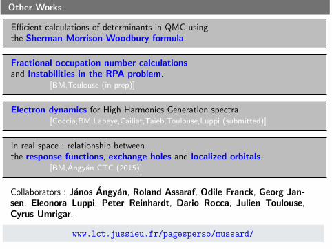
Other Works

Efficient calculations of determinants in QMC usingthe Sherman-Morrison-Woodbury formula.

Fractional occupation number calculationsand Instabilities in the RPA problem.

[BM,Toulouse (in prep)]

Electron dynamics for High Harmonics Generation spectra[Coccia,BM,Labeye,Caillat,Taieb,Toulouse,Luppi (submitted)]

In real space : relationship betweenthe response functions, exchange holes and localized orbitals.

[BM,Angyan CTC (2015)]

Collaborators : Janos Angyan, Roland Assaraf, Odile Franck, Georg Jan-sen, Eleonora Luppi, Peter Reinhardt, Dario Rocca, Julien Toulouse,Cyrus Umrigar.



Bastien Mussard · A short presentation (1) What I do : Quantum Mechanics I Wavefunction theories...

Documents

Transcript of Bastien Mussard · A short presentation (1) What I do : Quantum Mechanics I Wavefunction theories...