SPE/IADC 119882

Drilling Wells With Narrow Operating Windows Applying the MPD Constant Bottom Hole Pressure Technology – How Much the Temperature and Pressure Affects the Operation’s Design? M. Arnone, and P. Vieira, SPE, Weatherford International.

Copyright 2009, SPE/IADC Drilling Conference and Exhibition This paper was prepared for presentation at the SPE/IADC Drilling Conference and Exhibition held in Amsterdam, The Netherlands, 17–19 March 2009. This paper was selected for presentation by an SPE/IADC program committee following review of information contained in an abstract submitted by the author(s). Contents of the paper have not been reviewed by the Society of Petroleum Engineers or the International Association of Drilling Contractors and are subject to correction by the author(s). The material does not necessarily reflect any position of the Society of Petroleum Engineers or the International Association of Drilling Contractors, its officers, or members. Electronic reproduction, distribution, or storage of any part of this paper without the written consent of the Society of Petroleum Engineers or the International Association of Drilling Contractors is prohibited. Permission to reproduce in print is restricted to an abstract of not more than 300 words; illustrations may not be copied. The abstract must contain conspicuous acknowledgment of SPE/IADC copyright.

Abstract Narrow pore / fracture pressure gradient margins (operating window) is translated as a real drilling hazard scenario, where a slight change in the bottom hole pressure conditions can lead to an increase the Non Productive Time (NPT) due to the time spent in solve a possible fluid losses and/or gas kick situation, or even worst, dealing with occurrence of blowouts. In specific and non rare cases, deep formations with small gap between pore and fracture pressure are un-drillable with conventional drilling practices because the frictional losses pressure (difference between the dynamic and static pressure) is greater than the existent operating window. Constant Bottom Hole Pressure (CBHP), one of a number of variants of Managed Pressure Drilling (MPD) enables “walking the line” between pore and fracture pressure gradient. The objective is to drill with a fluid that bottom hole pressure is maintained constant, whether the fluid column is static or circulating. The loss of annulus flowing pressure when not circulating is counteracted by applied surface backpressure. The basic of Constant Bottom Hole Pressure (CBHP) methodology is to accurately determine the change in bottom hole pressure caused by dynamic effects and compensate with an equal change in annular wellhead pressure. The bottom hole temperature as well as the hydrostatic head of the drilling fluid column increases with the well depth and both parameters have opposing effect in the resultant static and dynamic equivalent density. An increase in the hydrostatic and dynamic pressures increases the equivalent fluid density due to compression but an increase in the temperature causes a reduction in the equivalent fluid density due to thermal expansion. Conventionally, these parameters considered together results in a cancellation of effects. In the reality, this assumption should be carefully reviewed. The effect of temperature in annular pressures, on a MPD CBHP operation through narrow operating windows, can not be ignored due to the potential impact. Precise estimation of static and dynamic equivalent fluid densities is of essential importance for a successful MPD CBHP operation through narrow operating windows. Introduction The IADC has recently updated the definition of Managed Pressure Drilling (MPD) as follow: MPD is an adaptive drilling process used to precisely control the annular pressure profile throughout the wellbore. The objectives are to ascertain the downhole pressure environment limits and to manage the annular hydraulic pressure profile accordingly. MPD is intended to avoid continuous influx of formation fluids to the surface. Any influx incidental to the operation will be safely contained using an appropriate process. The IADC definition for MPD also includes some key technical notes:

• MPD process employs a collection of tools and techniques which may mitigate the risks and costs associated with drilling wells that have narrow downhole environmental limits, by proactively managing

2 SPE/IADC 119882

the annular hydraulic pressure profile. • MPD may include control of back pressure, fluid density, fluid rheology, annular fluid level, circulating

friction, and hole geometry, or combinations thereof. • MPD may allow faster corrective action to deal with observed pressure variations. The ability to

dynamically control annular pressures facilitates drilling of what might otherwise be economically unattainable prospects.

At present date there are four recognized variations of MPD:

• Constant Bottom Hole Pressure (CBHP): Narrow Pore and fracture pressure gradient window present a drilling hazard. When the hole is being drilled or circulated, the additional circulating friction to hydrostatic head can result in formation fracture. When circulation in ceased, the hydrostatic pressure lies below the formation pore pressure. A kick-loss situation ensues, and nonproductive time (NPT), lost fluid cost and HSE risk escalate. This variation is applicable to avoid changes in Equivalent Circulating Density (ECD) by applying appropriate levels of surface backpressure, a technique that maintains constant the bottom hole pressure during the complete drilling operation.

• Pressurized Mud-Cap Drilling (PMCD): This variant of MPD enables the drilling process to continue without incurring the large drilling mud costs normally associated with losses, while also reducing well control risk resulting from difficulty in maintaining a fluid column as a primary barrier (no pore-facture pressure window is evident).

• Return Flow Control Drilling (HSE): Using an open to the atmosphere fluid return system when drilling with hazardous drilling fluids or in formations expected to have high concentrations of toxic gases, as hydrogen sulfide, raises health, safety and environmental concerns. The use of close system at surface and the right procedures reduces the risk to personnel, equipment and the environment from drilling and formation fluids and well control incidents.

• Dual Gradient (DG): The wellbore is drilled with two different annulus fluid gradients in place. Techniques to achieve a dual gradient include injecting a lower density fluid through a parasite string, through a concentric casing or actively pumping fluid returns from the seafloor through lines external to a seawater filled riser. In all cases the objective is to allow adjustment of the bottom hole pressure to within a predetermined range without changing the base weight of the drilling fluid.

Several un-drillable wells or extremely expensive wells can be easily drilled and profitable if the CBHP variant of MPD is used. In all the variants of MPD, but much more important in CBHP, an accurate estimation of equivalent circulating Density (ECD) and Bottom Hole Static and Circulating pressure are essential components of successful application of this technology. As the drilling fluid circulates through the wellbore and the hole drilled deeper, the fluid experiences different downhole conditions as a result in continuous changes in downhole pressure and temperature. In other words, the drilling fluid density measured at surface does not represent the drilling fluid density throughout the wellbore, and in consequence the static pressure exerted by the column of drilling fluid, the dynamic pressure exerted by the fluid while circulated and the frictional pressure losses estimation are affected by the effect of the real drilling fluid density (Demirdal, 2007). There are some real well cases where the operating window was not greater than 50 – 100 psi and the most efficient way how to drill through a section with that small difference between the pore and fracture pressure was to plan and apply MPD CBHP considering all the factors that use to affect the drilling fluid, as the formation pressure and temperature profile. Without these estimations, the result would be far from successful and dangerous situations as kick/losses scenarios incurred resulting in a wrong application of this technology. In this paper are presented the researches realized in terms of the drilling fluid density variation with pressure and temperature using laboratory test, analytical predictions of the drilling fluid circulating temperature, transient effects of the circulation on the drilling fluid density, MPD CBHP hydraulic simulations using the effect of temperature and pressure in the bottom hole circulating and static pressure determination and the operational procedures used to verify the hydraulic models during the application of this technology compensating at any time the usual error of use the same surface fluid density as constant in function of depth and time. In conclusion, in a narrow operating window environment, the consideration of the effect in the bottom hole circulating and static pressure by the temperature and pressure are extremely important in order to drill successfully a conventionally un-drillable well using MPD CBHP.

SPE/IADC 119882 3

Important Concepts Equivalent Static Density (ESD): the equivalent static density of a drilling fluid is an expression of the hydrostatic pressure term of the general equation (Ec. 1) exerted by a static column of fluid. Hydrostatic pressure is defined (Harris, 2005) as the pressure exerted at any point by a static column of liquid, and is a function of the density of the liquid and the height of the liquid column. Frequently, the calculation of the hydrostatic pressure is realized using the fluid density at standard conditions or at rig well site conditions. As the fluid density is affected by the formation pressure and temperature, the hydrostatic term calculation must be corrected using the variation in fluid density in order to obtain the real value of static bottom hole pressure (SBHP). The ESD is expressed in field units as follows:

hSBHP

ESD 052.0=ρ ,psi ……………………………(1)

Where the static bottom hole pressure (SBHP) is in psi and the static height of a static column of drilling fluid h in ft. Equivalent Circulating Density (ECD): this term is defined as the sum of the ESD of the drilling fluid and pressure loss in the annulus due to fluid flow. ECD is expressed in field units as follows:

hPfriction

ESDECD 052.0Δ

+= ρρ , psi …………………………(2)

Higher formation temperature cause thermal expansion of the drilling fluid and in consequence lower ESD and ECD, while higher formation pressures result in compression and increase in ESD and ECD. The effect of both (temperature and pressure), as opposite, are not necessarily canceled and the determination of the final effect is determinant at the moment when a MPD CBHP operation will be planned and applied.

The determination of the drilling fluid static and circulating temperature in function of depth During the drilling process, the fluid temperature at certain depth is not constant due to the thermal phenomena present during the circulation of the drilling fluid. There is heat transfer from the formation to the drilled hole due to the difference between the geothermal and the drilling fluid temperatures; this process can be analyzed in two parts: the first, the heat transfer between the fluid inside the drill string (moving from surface to bottom) and the fluid inside the annular space (moving from bottom to surface). Holmes and Swift developed a mathematical analytical model used today to predict the circulating drilling fluid temperature in stationary state in function of the depth inside the drill string and in the annular space while drilling or circulating the well. Even if there are several models more elaborated, normally needs solutions using numerical methods complicating the model. The results obtained by Holmes and Swift have been used in different situations and predicted successfully the bottom hole temperature verified using temperature logs. However, all the deductions and analytical expressions used to determine the drilling fluid temperature profile in the annular space have been used basically in vertical well. As is very common to find more applications of directional wells in the present, using the same methodology of Holmes and Swift, Acuña and Arnone obtained a mathematical expression adjusted to any well trajectory. These expressions are going to be used in this technical paper as reference as more general in terms of the well deviation and because as an analytical model, all the iterative calculations are avoided. The balance of energy conduces to the following differential equation to determine the temperature distribution in the annular space:

sa

lxt

lxta TGzcos1BeAe)L(T 21 +⎟⎟

⎠

⎞⎜⎜⎝

⎛+

−++= Ψ

δααδαδ ……………… (3)

This equation is analytically solved using simple calculation sheet and the solution will help to determine the fluid circulating temperature and in consequence the related affected density in order to establish the real Equivalent

4 SPE/IADC 119882

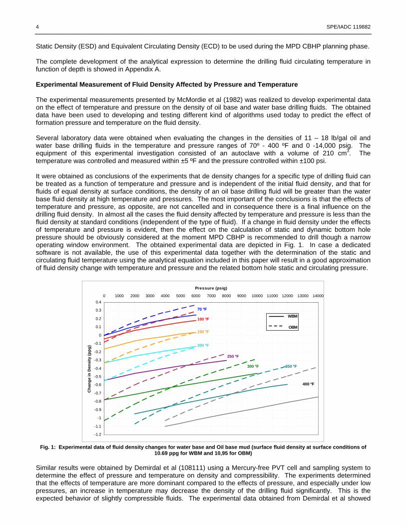
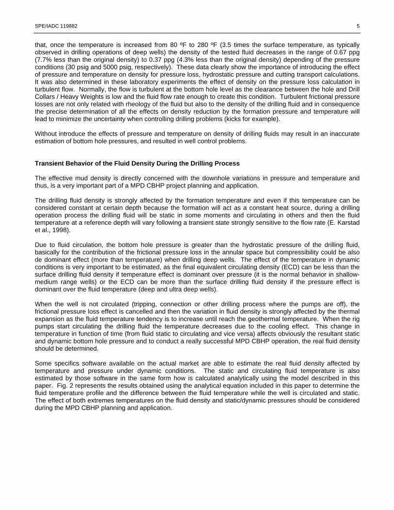
Static Density (ESD) and Equivalent Circulating Density (ECD) to be used during the MPD CBHP planning phase. The complete development of the analytical expression to determine the drilling fluid circulating temperature in function of depth is showed in Appendix A. Experimental Measurement of Fluid Density Affected by Pressure and Temperature The experimental measurements presented by McMordie et al (1982) was realized to develop experimental data on the effect of temperature and pressure on the density of oil base and water base drilling fluids. The obtained data have been used to developing and testing different kind of algorithms used today to predict the effect of formation pressure and temperature on the fluid density. Several laboratory data were obtained when evaluating the changes in the densities of 11 – 18 lb/gal oil and water base drilling fluids in the temperature and pressure ranges of 70º - 400 ºF and 0 -14,000 psig. The equipment of this experimental investigation consisted of an autoclave with a volume of 210 cm3. The temperature was controlled and measured within ±5 ºF and the pressure controlled within ±100 psi. It were obtained as conclusions of the experiments that de density changes for a specific type of drilling fluid can be treated as a function of temperature and pressure and is independent of the initial fluid density, and that for fluids of equal density at surface conditions, the density of an oil base drilling fluid will be greater than the water base fluid density at high temperature and pressures. The most important of the conclusions is that the effects of temperature and pressure, as opposite, are not cancelled and in consequence there is a final influence on the drilling fluid density. In almost all the cases the fluid density affected by temperature and pressure is less than the fluid density at standard conditions (independent of the type of fluid). If a change in fluid density under the effects of temperature and pressure is evident, then the effect on the calculation of static and dynamic bottom hole pressure should be obviously considered at the moment MPD CBHP is recommended to drill though a narrow operating window environment. The obtained experimental data are depicted in Fig. 1. In case a dedicated software is not available, the use of this experimental data together with the determination of the static and circulating fluid temperature using the analytical equation included in this paper will result in a good approximation of fluid density change with temperature and pressure and the related bottom hole static and circulating pressure.

-1.2

-1.1

-1

-0.9

-0.8

-0.7

-0.6

-0.5

-0.4

-0.3

-0.2

-0.1

0

0.1

0.2

0.3

0.40 1000 2000 3000 4000 5000 6000 7000 8000 9000 10000 11000 12000 13000 14000

Pressure (psig)

Cha

nge

in D

ensi

ty (p

pg)

70 ºF

100 ºF

150 ºF

200 ºF

250 ºF

300 ºF 350 ºF

400 ºF

WBM

OBM

Fig. 1: Experimental data of fluid density changes for water base and Oil base mud (surface fluid density at surface conditions of

10.69 ppg for WBM and 10,95 for OBM) Similar results were obtained by Demirdal et al (108111) using a Mercury-free PVT cell and sampling system to determine the effect of pressure and temperature on density and compressibility. The experiments determined that the effects of temperature are more dominant compared to the effects of pressure, and especially under low pressures, an increase in temperature may decrease the density of the drilling fluid significantly. This is the expected behavior of slightly compressible fluids. The experimental data obtained from Demirdal et al showed

SPE/IADC 119882 5

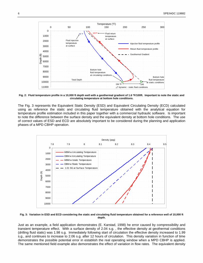
that, once the temperature is increased from 80 ºF to 280 ºF (3.5 times the surface temperature, as typically observed in drilling operations of deep wells) the density of the tested fluid decreases in the range of 0.67 ppg (7.7% less than the original density) to 0.37 ppg (4.3% less than the original density) depending of the pressure conditions (30 psig and 5000 psig, respectively). These data clearly show the importance of introducing the effect of pressure and temperature on density for pressure loss, hydrostatic pressure and cutting transport calculations. It was also determined in these laboratory experiments the effect of density on the pressure loss calculation in turbulent flow. Normally, the flow is turbulent at the bottom hole level as the clearance between the hole and Drill Collars / Heavy Weights is low and the fluid flow rate enough to create this condition. Turbulent frictional pressure losses are not only related with rheology of the fluid but also to the density of the drilling fluid and in consequence the precise determination of all the effects on density reduction by the formation pressure and temperature will lead to minimize the uncertainty when controlling drilling problems (kicks for example). Without introduce the effects of pressure and temperature on density of drilling fluids may result in an inaccurate estimation of bottom hole pressures, and resulted in well control problems. Transient Behavior of the Fluid Density During the Drilling Process The effective mud density is directly concerned with the downhole variations in pressure and temperature and thus, is a very important part of a MPD CBHP project planning and application. The drilling fluid density is strongly affected by the formation temperature and even if this temperature can be considered constant at certain depth because the formation will act as a constant heat source, during a drilling operation process the drilling fluid will be static in some moments and circulating in others and then the fluid temperature at a reference depth will vary following a transient state strongly sensitive to the flow rate (E. Karstad et al., 1998). Due to fluid circulation, the bottom hole pressure is greater than the hydrostatic pressure of the drilling fluid, basically for the contribution of the frictional pressure loss in the annular space but compressibility could be also de dominant effect (more than temperature) when drilling deep wells. The effect of the temperature in dynamic conditions is very important to be estimated, as the final equivalent circulating density (ECD) can be less than the surface drilling fluid density if temperature effect is dominant over pressure (it is the normal behavior in shallow-medium range wells) or the ECD can be more than the surface drilling fluid density if the pressure effect is dominant over the fluid temperature (deep and ultra deep wells). When the well is not circulated (tripping, connection or other drilling process where the pumps are off), the frictional pressure loss effect is cancelled and then the variation in fluid density is strongly affected by the thermal expansion as the fluid temperature tendency is to increase until reach the geothermal temperature. When the rig pumps start circulating the drilling fluid the temperature decreases due to the cooling effect. This change in temperature in function of time (from fluid static to circulating and vice versa) affects obviously the resultant static and dynamic bottom hole pressure and to conduct a really successful MPD CBHP operation, the real fluid density should be determined. Some specifics software available on the actual market are able to estimate the real fluid density affected by temperature and pressure under dynamic conditions. The static and circulating fluid temperature is also estimated by those software in the same form how is calculated analytically using the model described in this paper. Fig. 2 represents the results obtained using the analytical equation included in this paper to determine the fluid temperature profile and the difference between the fluid temperature while the well is circulated and static. The effect of both extremes temperatures on the fluid density and static/dynamic pressures should be considered during the MPD CBHP planning and application.

6 SPE/IADC 119882

101ºF

194 ºF 245

0

1000

2000

3000

4000

5000

6000

7000

8000

9000

10000

11000

0 50 100 150 200 250 300Temperature (°F)

Dep

th (f

t)

Fluid returntemperatureat surface

95 °F

Total Depth

Injection fluid temperature profile

Return fluid temperature profile

Geothermal Gradient

Bottom hole fluid temperature

at static conditions

Bottom holefluid temperatureat circulating conditions

Fluid injectiontemperatureat surface

T dynamic - static fluid conditionsΔ Fig. 2: Fluid temperature profile in a 10,000 ft depth well with a geothermal gradient of 1.6 ºF/100ft. Important to note the static and

circulating temperature at bottom hole conditions. The Fig. 3 represents the Equivalent Static Density (ESD) and Equivalent Circulating Density (ECD) calculated using as reference the static and circulating fluid temperature obtained with the analytical equation for temperature profile estimation included in this paper together with a commercial hydraulic software. Is important to note the difference between the surface density and the equivalent density at bottom hole conditions. The use of correct values of ESD and ECD are absolutely important to be considered during the planning and application phases of a MPD CBHP operation.

0

1000

2000

3000

4000

5000

6000

7000

8000

9000

10000

7.8 7.9 8 8.1 8.2 8.3 8.4 8.5

Density (ppg)

Dep

th (f

t)

WBM w /circulating Temperature

OBM w /circulating Temperature

WBM w /static Temperature

OBM w /Static Temperature

1.01 SG at Surface Temperature

Fig. 3: Variation in ESD and ECD considering the static and circulating fluid temperature obtained for a reference well of 10,000 ft depth.

Just as an example, a field application demonstrates (E. Karstad, 1998) he error caused by compressibility and transient temperature effect. With a surface density of 2.04 s.g. , the effective density at geothermal conditions (drilling fluid static) was 1.98 s.g. Immediately following start of circulation the effective density increased to 1.99 s.g., and continues to increase to 2.06 s.g. after 12 hours of circulation. This density variation in function of time demonstrates the possible potential error in establish the real operating window when a MPD CBHP is applied. The same mentioned field example also demonstrates the effect of variation in flow rates. The equivalent density

SPE/IADC 119882 7

changes more rapid for higher circulation rates and it tends to stabilize at higher value. For most practical purposes the equivalent density has stabilized within 12 hours of drilling fluid circulation. Technical Considerations for MPD CBHP planning

The MPD variant of Constant Bottom Hole Pressure (CBHP) enables “Walking the Line” between the pore and fracture pressure gradient while drilling the subject formation where severe losses and gas kicks are expected, having applicability also in exploratory wells where the operating window has high degree of uncertainty and in cases where a low reservoir damaging drilling fluid wants to be used but the maximum fluid density reachable is below the maximum expected formation pressure. The objective is to drill using a combination of such a mud weight and especial procedures, so that the bottom hole pressure is maintained constant, under dynamic or static conditions, and as demonstrated, considering the effects of formation temperature and pressure on the variations of drilling fluid properties as the density.

In addition, changing the Equivalent Mud Weight is instantaneous by the simple action of adjusting the circulation pump rate or the back pressure on the MPD choke in order to keep the control of the pressure profile in the wellbore, therefore any down hole hazardous conditions will be reduced.

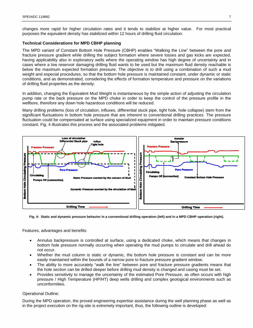
Many drilling problems (loss of circulation, influxes, differential stuck pipe, tight hole, hole collapse) stem from the significant fluctuations in bottom hole pressure that are inherent to conventional drilling practices. The pressure fluctuation could be compensated at surface using specialized equipment in order to maintain pressure conditions constant. Fig. 4 illustrates this process and the associated problems mitigated.

Bot

tom

Hol

e C

ircul

atin

g Pr

essu

re

Drilling Time

Fracture Pressure

Pore Pressure

Static Pressure exerted by the column of Mud

Dynamic Pressure exerted by the circulation of Mud

Circulating

Pumps Off (connection)

Loss of circulationDifferential Stuck pipe Influx

Tight hole

Bot

tom

Hol

e C

ircul

atin

g Pr

essu

re

Drilling Time

Fracture Pressure

Pore Pressure

Static Pressure exerted by the column of Mud

Dynamic Pressure exerted by the circulation of Mud

Circulating

Pumps Off (connection)

Loss of circulationDifferential Stuck pipe Influx

Tight holeB

otto

m H

ole

Circ

ulat

ing

Pres

sure

Drilling Time

Fracture Pressure

Pore PressureCirculating

Pumps Off (connection)

AnnularBackpressure

Constant Bottom Hole Pressure

Bot

tom

Hol

e C

ircul

atin

g Pr

essu

re

Drilling Time

Fracture Pressure

Pore PressureCirculating

Pumps Off (connection)

AnnularBackpressure

Constant Bottom Hole Pressure

Bot

tom

Hol

e C

ircul

atin

g Pr

essu

re

Drilling Time

Fracture Pressure

Pore Pressure

Static Pressure exerted by the column of Mud

Dynamic Pressure exerted by the circulation of Mud

Circulating

Pumps Off (connection)

Loss of circulationDifferential Stuck pipe Influx

Tight hole

Bot

tom

Hol

e C

ircul

atin

g Pr

essu

re

Drilling Time

Fracture Pressure

Pore Pressure

Static Pressure exerted by the column of Mud

Dynamic Pressure exerted by the circulation of Mud

Circulating

Pumps Off (connection)

Loss of circulationDifferential Stuck pipe Influx

Tight holeB

otto

m H

ole

Circ

ulat

ing

Pres

sure

Drilling Time

Fracture Pressure

Pore PressureCirculating

AnnularBackpressure

Pumps Off (connection) Constant Bottom Hole Pressure

Bot

tom

Hol

e C

ircul

atin

g Pr

essu

re

Drilling Time

Fracture Pressure

Pore PressureCirculating

AnnularBackpressure

Pumps Off (connection) Constant Bottom Hole Pressure

Fig. 4: Static and dynamic pressure behavior in a conventional drilling operation (left) and in a MPD CBHP operation (right). Features, advantages and benefits:

• Annulus backpressure is controlled at surface, using a dedicated choke, which means that changes in bottom hole pressure normally occurring when operating the mud pumps to circulate and drill ahead do not occur.

• Whether the mud column is static or dynamic, the bottom hole pressure is constant and can be more easily maintained within the bounds of a narrow pore to fracture pressure gradient window.

• The ability to more accurately “walk the line” between pore and fracture pressure gradients means that the hole section can be drilled deeper before drilling mud density is changed and casing must be set.

• Provides sensitivity to manage the uncertainty of the estimated Pore Pressure, as often occurs with high pressure / High Temperature (HP/HT) deep wells drilling and complex geological environments such as unconformities.

Operational Outline:

During the MPD operation, the proved engineering expertise assistance during the well planning phase as well as in the project execution on the rig-site is extremely important, thus, the following outline is developed:

8 SPE/IADC 119882

• The hydraulic flow modeling will determine the range or operational envelope within the limits of the pressure profile that is required to maintain a constant BHP. It establishes the maximum surface pressures or circulation pump rates required to accomplish an acceptable degree of overbalance during all the drilling procedures. Considering obviously the effect of temperature and pressure on the drilling fluid properties.

• The MPD CBHP equipment is basically formed by: A suitably specified Rotating Control device (RCD), a MPD choke manifold, a specific return line flow-meter if there is suspect of gas influx into the well and drill string floats.

• Specific operating procedures must be developed to consider events like connections, trips, coring, well control, etc., according to the drilling conditions to be experienced.

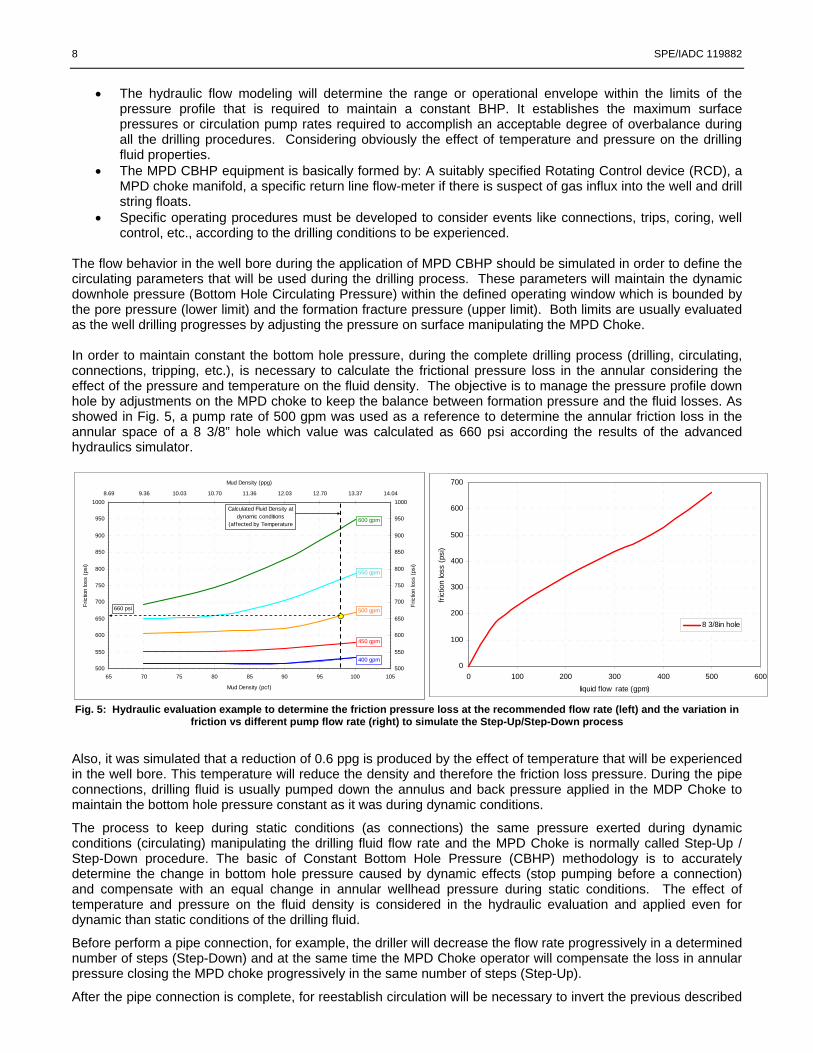
The flow behavior in the well bore during the application of MPD CBHP should be simulated in order to define the circulating parameters that will be used during the drilling process. These parameters will maintain the dynamic downhole pressure (Bottom Hole Circulating Pressure) within the defined operating window which is bounded by the pore pressure (lower limit) and the formation fracture pressure (upper limit). Both limits are usually evaluated as the well drilling progresses by adjusting the pressure on surface manipulating the MPD Choke. In order to maintain constant the bottom hole pressure, during the complete drilling process (drilling, circulating, connections, tripping, etc.), is necessary to calculate the frictional pressure loss in the annular considering the effect of the pressure and temperature on the fluid density. The objective is to manage the pressure profile down hole by adjustments on the MPD choke to keep the balance between formation pressure and the fluid losses. As showed in Fig. 5, a pump rate of 500 gpm was used as a reference to determine the annular friction loss in the annular space of a 8 3/8” hole which value was calculated as 660 psi according the results of the advanced hydraulics simulator.

500

550

600

650

700

750

800

850

900

950

1000

65 70 75 80 85 90 95 100 105

Mud Density (pcf)

Fric

tion

loss

(psi

)

500

550

600

650

700

750

800

850

900

950

10008.69 9.36 10.03 10.70 11.36 12.03 12.70 13.37 14.04

Mud Density (ppg)

Fric

tion

loss

(psi

)

400 gpm

450 gpm

500 gpm

550 gpm

600 gpm

Calculated Fluid Density at dynamic conditions

(affected by Temperature d P )

660 psi

0

100

200

300

400

500

600

700

0 100 200 300 400 500 600liquid flow rate (gpm)

frict

ion

loss

(psi

)

8 3/8in hole

500

550

600

650

700

750

800

850

900

950

1000

65 70 75 80 85 90 95 100 105

Mud Density (pcf)

Fric

tion

loss

(psi

)

500

550

600

650

700

750

800

850

900

950

10008.69 9.36 10.03 10.70 11.36 12.03 12.70 13.37 14.04

Mud Density (ppg)

Fric

tion

loss

(psi

)

400 gpm

450 gpm

500 gpm

550 gpm

600 gpm

Calculated Fluid Density at dynamic conditions

(affected by Temperature d P )

660 psi

0

100

200

300

400

500

600

700

0 100 200 300 400 500 600liquid flow rate (gpm)

frict

ion

loss

(psi

)

8 3/8in hole

Fig. 5: Hydraulic evaluation example to determine the friction pressure loss at the recommended flow rate (left) and the variation in

friction vs different pump flow rate (right) to simulate the Step-Up/Step-Down process

Also, it was simulated that a reduction of 0.6 ppg is produced by the effect of temperature that will be experienced in the well bore. This temperature will reduce the density and therefore the friction loss pressure. During the pipe connections, drilling fluid is usually pumped down the annulus and back pressure applied in the MDP Choke to maintain the bottom hole pressure constant as it was during dynamic conditions.

The process to keep during static conditions (as connections) the same pressure exerted during dynamic conditions (circulating) manipulating the drilling fluid flow rate and the MPD Choke is normally called Step-Up / Step-Down procedure. The basic of Constant Bottom Hole Pressure (CBHP) methodology is to accurately determine the change in bottom hole pressure caused by dynamic effects (stop pumping before a connection) and compensate with an equal change in annular wellhead pressure during static conditions. The effect of temperature and pressure on the fluid density is considered in the hydraulic evaluation and applied even for dynamic than static conditions of the drilling fluid.

Before perform a pipe connection, for example, the driller will decrease the flow rate progressively in a determined number of steps (Step-Down) and at the same time the MPD Choke operator will compensate the loss in annular pressure closing the MPD choke progressively in the same number of steps (Step-Up).

After the pipe connection is complete, for reestablish circulation will be necessary to invert the previous described

SPE/IADC 119882 9

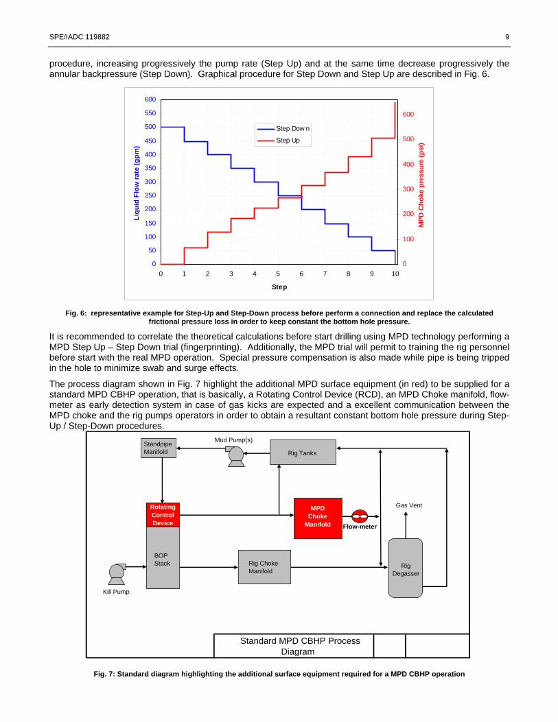
procedure, increasing progressively the pump rate (Step Up) and at the same time decrease progressively the annular backpressure (Step Down). Graphical procedure for Step Down and Step Up are described in Fig. 6.

0

50

100

150

200

250

300

350

400

450

500

550

600

0 1 2 3 4 5 6 7 8 9 10

Step

Liqu

id F

low

rate

(gpm

)

0

100

200

300

400

500

600

MPD

Cho

ke p

ress

ure

(psi

)

Step Dow n

Step Up

Fig. 6: representative example for Step-Up and Step-Down process before perform a connection and replace the calculated

frictional pressure loss in order to keep constant the bottom hole pressure.

It is recommended to correlate the theoretical calculations before start drilling using MPD technology performing a MPD Step Up – Step Down trial (fingerprinting). Additionally, the MPD trial will permit to training the rig personnel before start with the real MPD operation. Special pressure compensation is also made while pipe is being tripped in the hole to minimize swab and surge effects.

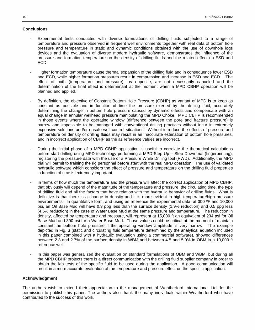
The process diagram shown in Fig. 7 highlight the additional MPD surface equipment (in red) to be supplied for a standard MPD CBHP operation, that is basically, a Rotating Control Device (RCD), an MPD Choke manifold, flow-meter as early detection system in case of gas kicks are expected and a excellent communication between the MPD choke and the rig pumps operators in order to obtain a resultant constant bottom hole pressure during Step-Up / Step-Down procedures.

RigDegasser

Rig Tanks

Rig ChokeManifold

MPD Choke

Manifold

RotatingControlDevice

BOPStack

Gas Vent

StandpipeManifold

Mud Pump(s)

Kill Pump

Standard MPD CBHP Process Diagram

Flow-meter

Fig. 7: Standard diagram highlighting the additional surface equipment required for a MPD CBHP operation

10 SPE/IADC 119882

Conclusions

- Experimental tests conducted with diverse formulations of drilling fluids subjected to a range of temperature and pressure observed in frequent well environments together with real data of bottom hole pressure and temperature in static and dynamic conditions obtained with the use of downhole logs devices and the evaluation of diverse modern hydraulic software, demonstrates the influence of the pressure and formation temperature on the density of drilling fluids and the related effect on ESD and ECD.

- Higher formation temperature cause thermal expansion of the drilling fluid and in consequence lower ESD

and ECD, while higher formation pressures result in compression and increase in ESD and ECD. The effect of both (temperature and pressure), as opposite, are not necessarily canceled and the determination of the final effect is determinant at the moment when a MPD CBHP operation will be planned and applied.

- By definition, the objective of Constant Bottom Hole Pressure (CBHP) as variant of MPD is to keep as

constant as possible and in function of time the pressure exerted by the drilling fluid, accurately determining the change in bottom hole pressure caused by dynamic effects and compensate with an equal change in annular wellhead pressure manipulating the MPD Choke. MPD CBHP is recommended in those events where the operating window (difference between the pore and fracture pressure) is narrow and impossible to be managed with conventional drilling practices without incur in extremely expensive solutions and/or unsafe well control situations. Without introduce the effects of pressure and temperature on density of drilling fluids may result in an inaccurate estimation of bottom hole pressures, and in incorrect application of CBHP as the as reference values are incorrect.

- During the initial phase of a MPD CBHP application is useful to correlate the theoretical calculations

before start drilling using MPD technology performing a MPD Step Up – Step Down trial (fingerprinting), registering the pressure data with the use of a Pressure While Drilling tool (PWD). Additionally, the MPD trial will permit to training the rig personnel before start with the real MPD operation. The use of validated hydraulic software which considers the effect of pressure and temperature on the drilling fluid properties in function of time is extremely important.

- In terms of how much the temperature and the pressure will affect the correct application of MPD CBHP,

that obviously will depend of the magnitude of the temperature and pressure, the circulating time, the type of drilling fluid and all the factors that have relation with the hydraulic behavior of drilling fluids. What is definitive is that there is a change in density and it is more evident in high temperature/high pressure environments. In quantitative form, and using as reference the experimental data, at 300 ºF and 10,000 psi, an Oil Base Mud will have 0.3 ppg less than the surface density (1.9% reduction) and 0.5 ppg less (4.5% reduction) in the case of Water Base Mud at the same pressure and temperature. The reduction in density, affected by temperature and pressure, will represent at 15,000 ft an equivalent of 234 psi for Oil Base Mud and 390 psi for a Water Base Mud. Those values could be critical at the moment of maintain constant the bottom hole pressure if the operating window amplitude is very narrow. The example depicted in Fig. 3 (static and circulating fluid temperature determined by the analytical equation included in this paper combined with a hydraulic evaluation using a commercial software), showed differences between 2.3 and 2.7% of the surface density in WBM and between 4.5 and 5.9% in OBM in a 10,000 ft reference well.

- In this paper was generalized the evaluation on standard formulations of OBM and WBM, but during all

the MPD CBHP projects there is a direct communication with the drilling fluid supplier company in order to obtain the lab tests of the specific fluid to be used during the application. A good communication will result in a more accurate evaluation of the temperature and pressure effect on the specific application.

Acknowledgment The authors wish to extend their appreciation to the management of Weatherford International Ltd. for the permission to publish this paper. The authors also thank the many individuals within Weatherford who have contributed to the success of this work.

SPE/IADC 119882 11

References Arnone M.: “Analysis and Simulation of the Gas Cut Mud Phenomena in the Drilling Operations of Directional Wells”, Master Science Thesis, presented to UCV, Caracas, Venezuela, 16 December 2003. Bjørkevoll K.S., Anfinsen T., Merlo A., Eriksen N. and Olsen E.: “Analysis of extended reach Drilling data Using an Advanced Pressure and Temperature Model”, IADC/SPE 62728, presented at the 2000 IADC/SPE Asia Pacific drilling Technology held in Kuala Lumpur, Malaysia, 11-13 September 2000. Bourgoyne Jr. A., Chenevert M., Millheim K. and Young Jr. F.S.: “ Applied Drilling Engineering”, SPE Textbook Series, Vol. 2, Chapter 4, 1991. Demirdal B., Miska S. and Takach N.: “Drilling Fluids Rheological and Volumetric Characterization Under Downhole Conditions”, SPE 108111, presented at the 2007 SPE Latin American and Caribbean Petroleum Engineering Conference held in Buenos Aires, Argentina, 15-18 April 2007. Foster J.K. and Steiner A.: “The Use of MPD and an Unweighted Fluid system for drilling ROP Improvement”, IADC/SPE 108343, presented at the 2007 IADC/SPE Managed Pressure Drilling and Underbalanced Operations Conference and Exhibition held in Galveston, Texas, U.S.A., 28-29 March 2007. Gau E., Booth M. and MacBeath N.: “Continued Improvements on High-Pressure/High-Temperature Drilling Performance on Wells With Extremelly Narrow Drilling Windows – Experiences From Mud Formulation to operational Practices, Shearwater Project”, IADC/SPE 59175, presented at the 2000 IADC/SPE Drilling Conference held in New Orleans, Louisiana, U.S.A., 23-25 February 2000. Hannegan D. and Fisher K.: “Managed Pressure Drilling in Marine Environments”, IPTC 10173, presented at the International Petroleum Technology Conference held in Doha, Qatar, 21-23 November 2005. Harris O.O. and Osisanya S.O.: “Evaluation of Equivalent Circulating Density of Drilling Fluids Under High-Pressure/High-Temperature Conditions”, SPE 97018, presented at the 2005 SPE Annual Technical Conference and Exhibition held in Dallas, Texas, U.S.A., 9-12 October 2005. International Association of Drilling Contractors (IADC), UBO and MPD Committee. Karstad E. and Aadnøy B.: “Density Behavior of Drilling Fluids During High Pressure High Temperature Drilling Operations”, IADC/SPE 47806, presented at the 1998 IADC/SPE Asia Pacific Drilling Technology Conference held in Jakarta, Indonesia, 7-9 September 1998. McMordie W.C., Bland R.G. and Hauser J.M.: “Effect of Temperature and Pressure on the Density of Drilling Fluids”, SPE 11114, presented at the 57th Annual Fall Conference and Exhibition of the Society of Petroleum Engineers of AIME held in New Orleans, LA., U.S.A., 26-29 September 1982. Osman E.A. and Aggour M.A.: “Determination of Drilling Mud Density Change with Pressure and Temperature Made Simple and Accurate by ANN”, SPE 81422, presented at the SPE 13th Middle east Oil Show and Conference held in Bahrain 5-8 April 2003. Nomenclature CBHP = Constant Bottom Hole Pressure Cp = Specific Heat Capacity D = Diameter, in ESD = Equivalent Static Density, ppg ECD = Equivalent Circulating Density, ppg G = Geothermal gradient, ºF/100 ft h = Depth, ft HP/HT = High Pressure / High Temperature L = Length, ft MPD = Managed Pressure Drilling m = Mass Flow Rate OBM = Oil Base Mud q = Heat Transfer

12 SPE/IADC 119882

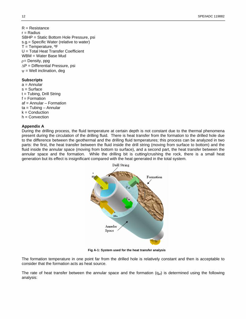
R = Resistance r = Radius SBHP = Static Bottom Hole Pressure, psi s.g.= Specific Water (relative to water) T = Temperature, ºF U = Total Heat Transfer Coefficient WBM = Water Base Mud ρ= Density, ppg ΔP = Differential Pressure, psi ψ = Well inclination, deg Subscripts a = Annular s = Surface t = Tubing, Drill String f = Formation af = Annular – Formation ta = Tubing – Annular k = Conduction h = Convection Appendix A During the drilling process, the fluid temperature at certain depth is not constant due to the thermal phenomena present during the circulation of the drilling fluid. There is heat transfer from the formation to the drilled hole due to the difference between the geothermal and the drilling fluid temperatures; this process can be analyzed in two parts: the first, the heat transfer between the fluid inside the drill string (moving from surface to bottom) and the fluid inside the annular space (moving from bottom to surface), and a second part, the heat transfer between the annular space and the formation. While the drilling bit is cutting/crushing the rock, there is a small heat generation but its effect is insignificant compared with the heat generated in the total system.

Fig A-1: System used for the heat transfer analysis

The formation temperature in one point far from the drilled hole is relatively constant and then is acceptable to consider that the formation acts as heat source. The rate of heat transfer between the annular space and the formation (qaf) is determined using the following analysis:

SPE/IADC 119882 13

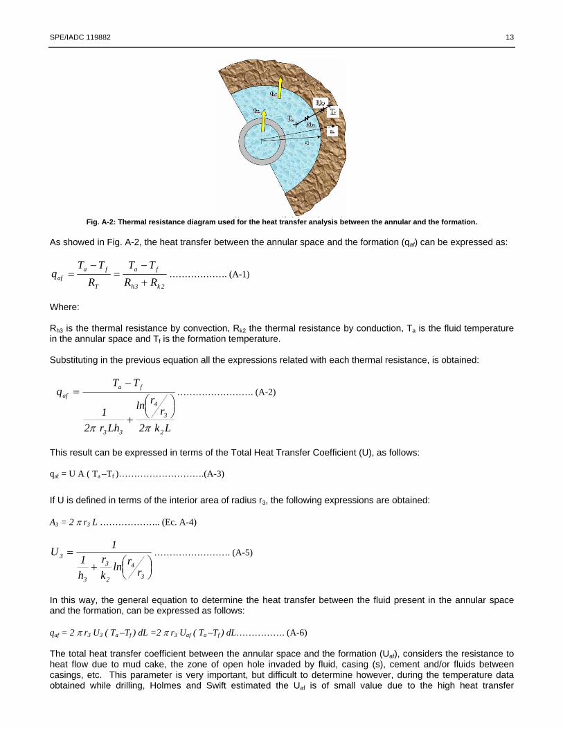
Fig. A-2: Thermal resistance diagram used for the heat transfer analysis between the annular and the formation.

As showed in Fig. A-2, the heat transfer between the annular space and the formation (qaf) can be expressed as:

2k3h

fa

T

faaf RR

TTR

TTq

+

−=

−= ………………. (A-1)

Where: Rh3 is the thermal resistance by convection, Rk2 the thermal resistance by conduction, Ta is the fluid temperature in the annular space and Tf is the formation temperature. Substituting in the previous equation all the expressions related with each thermal resistance, is obtained:

Lk2r

rln

Lhr21

TTq

2

3

4

33

faaf

ππ

⎟⎠⎞⎜

⎝⎛

+

−= ……………………. (A-2)

This result can be expressed in terms of the Total Heat Transfer Coefficient (U), as follows: qaf = U A ( Ta –Tf )……………………….(A-3)

If U is defined in terms of the interior area of radius r3, the following expressions are obtained: A3 = 2 π r3 L ……………….. (Ec. A-4)

⎟⎠⎞⎜

⎝⎛+

=

3

4

2

3

3

3

rrln

kr

h1

1U ……………………. (A-5)

In this way, the general equation to determine the heat transfer between the fluid present in the annular space and the formation, can be expressed as follows: qaf = 2 π r3 U3 ( Ta –Tf ) dL =2 π r3 Uaf ( Ta –Tf ) dL……………. (A-6) The total heat transfer coefficient between the annular space and the formation (Uaf), considers the resistance to heat flow due to mud cake, the zone of open hole invaded by fluid, casing (s), cement and/or fluids between casings, etc. This parameter is very important, but difficult to determine however, during the temperature data obtained while drilling, Holmes and Swift estimated the Uaf is of small value due to the high heat transfer

14 SPE/IADC 119882

resistance by the rock. They determined an average value for Uaf of 5.68 W/m2K (1 BTU/h ft2 F) The heat transfer between the fluid inside the drill string and the fluid in the annular space, can be determined using the following analysis:

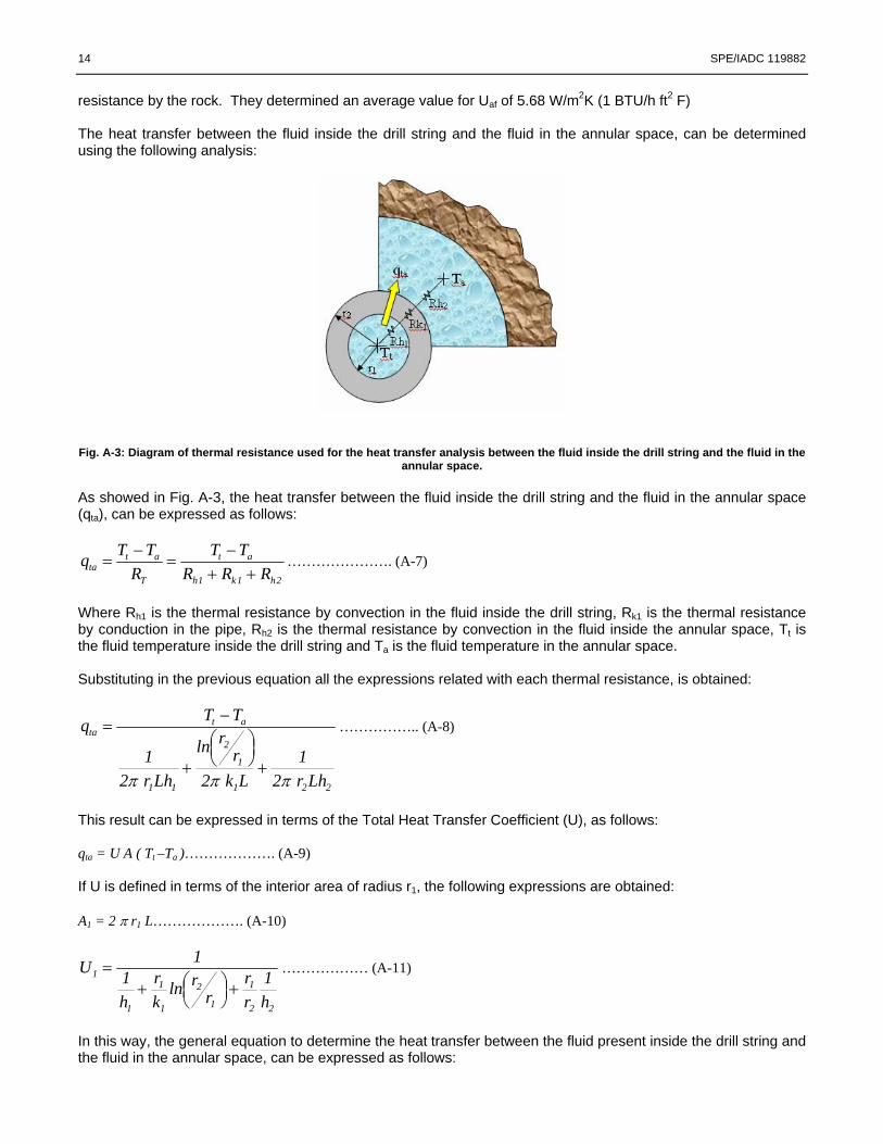
Fig. A-3: Diagram of thermal resistance used for the heat transfer analysis between the fluid inside the drill string and the fluid in the

annular space. As showed in Fig. A-3, the heat transfer between the fluid inside the drill string and the fluid in the annular space (qta), can be expressed as follows:

2h1k1h

at

T

atta RRR

TTR

TTq++

−=

−= …………………. (A-7)

Where Rh1 is the thermal resistance by convection in the fluid inside the drill string, Rk1 is the thermal resistance by conduction in the pipe, Rh2 is the thermal resistance by convection in the fluid inside the annular space, Tt is the fluid temperature inside the drill string and Ta is the fluid temperature in the annular space. Substituting in the previous equation all the expressions related with each thermal resistance, is obtained:

221

1

2

11

atta

Lhr21

Lk2r

rln

Lhr21

TTq

πππ+

⎟⎠⎞⎜

⎝⎛

+

−= …………….. (A-8)

This result can be expressed in terms of the Total Heat Transfer Coefficient (U), as follows: qta = U A ( Tt –Ta )………………. (A-9) If U is defined in terms of the interior area of radius r1, the following expressions are obtained: A1 = 2 π r1 L………………. (A-10)

22

1

1

2

1

1

1

1

h1

rr

rrln

kr

h1

1U+⎟

⎠⎞⎜

⎝⎛+

= ……………… (A-11)

In this way, the general equation to determine the heat transfer between the fluid present inside the drill string and the fluid in the annular space, can be expressed as follows:

SPE/IADC 119882 15

qta = 2 π r1 U1 ( Tt -Ta ) dL = 2 π r1 Uta ( Tt -Ta ) dL………………… (A-12)

Same as was expressed in the case of heat flow between the annular space and the formation, the total heat transfer coefficient between the fluid inside the drill string and the fluid in the annular space is difficult to determine. In the sensibilities realized by Holmes and Swift to simulate the circulating fluid temperature profile, it was used an average of Uta of 170 W/m2K (30 BTU/h ft2 F). The heat accumulation by the fluid in the annular space between the depths L and (L + dL) is expressed by:

)TT(cmqq dLLa

Laapa

dLLa

La

+•

+ −=− …………….. (A-13)

Where Cpa is the specific heat capacity of the fluid in the annular space, Ta the fluid temperature in the annular space evaluated between the depths L and L+dL. "ma” is the mass flow rate of annular fluid. Combining equations is obtained the total heat transferred through the annular space:

)TT(UD)TT(UDdLdT

cm faafhattata

apa −=−+•

ππ …………….. (A-14)

The formation temperature can be obtained using the following expressions: Tf = Ts + Gh ………………………… (A-15) Where Tf is the formation temperature, Ts the surface temperature of the fluid, G is the geothermal gradient and h the true vertical depth. A similar development for the fluid inside the drill string is obtained using the following heat balance:

)TT(UDdLdT

cm attatt

tpt −−=•

π ……………… (A-16)

Where Cpt is the specific heat capacity of the fluid inside the drill string, Ta is the fluid temperature in the annular space, Tt is the fluid temperature inside the drill string and “mt” is the mass flow rate of the fluid inside the drill string. Solution of the differential equations system Before proceed to obtain a mathematical expression to determine analytically the fluid temperature in function of depth, is convenient to use the following considerations:

- The diameter of drill string (Dt) and Dh (hole diameter) are function of L as the drill string use to have components of different diameter and the drilled hole/casings have different diameter, however dDt/dL = dDh/dL = 0 as the magnitudes are constant by section.

- The dog leg severity (in case of directional wells) can be low in terms that d2z/dL2 can be approximately zero. This consideration is true in straight sections of the hole even vertical, inclined or horizontal. In curve sections d2z/dl2 = -senψ/R, that can be approximately zero in long radius wells. For this analytical deduction, it will be considered, in case of deviated wells, that the build up rate is low.

With the described considerations, Holmes and swift developed a mathematical analytical model used today to predict the circulating drilling fluid temperature in stationary state in function of the depth inside the drill string and in the annular space while drilling or circulating the well. Even if there are several models more elaborated, normally needs solutions using numerical methods complicating the model. The results obtained by Holmes and Swift have been used in different situations and predicted successfully the bottom hole temperature verified using temperature logs. However, all the deductions and analytical expressions used to determine the drilling fluid temperature profile in the annular space have been used basically in vertical well. As is very common to find more applications of directional wells in the present, using the same methodology of Holmes and Swift, Acuña and

16 SPE/IADC 119882

Arnone obtained a mathematical expression adjusted to vertical and deviated wells. These expressions are going to be used in this technical paper as reference as more general in terms of the well deviation and because as a analytical model, all the iterative calculations are avoided. The balance of energy conduces to the following differential equation to determine the temperature distribution in the annular space.

fatf

aaata

att2a

2

TdL

dTT

dLdT

)(dL

Tdδδδδδδαδδ −−=−−−+ ………………… (A-17 )

Where:

tt

tatt

cm

hD•=

πδ ………..………… (A-18)

aa

afha

cm

hD•=

πδ ………………… (A-19)

aa

tt

cm

cm•

•

=α …………………… (A-20)

This equation was developed assuming that the physical and thermal properties of the formation does not vary with the temperature, the heat is transferred radially inside the formation and that the heat transfer in the hole is quicker compared with the heat transfer to the formation and in conclusion the solutions can be represented in stationary state. With the assumptions mentioned, equation 92 is linear of constant coefficients and the solution conduces to the following analytical expression of the fluid temperature in the annular space in function of the temperature:

sa

lxt

lxta TGzcos1BeAe)L(T 21 +⎟⎟

⎠

⎞⎜⎜⎝

⎛+

−++= Ψ

δααδαδ ………………… (A-21)

Where:

x1,2 = [ ]{ })1(2)1()1(21

tat2ata −+++±−+ αδδαδδαδδ ………………… (A-22)

There are several values for the constants A and B due to “da” and “dt” represents discontinue functions. The boundary conditions in each point of the discontinuity are represented equalizing the temperatures from one side and the other of the discontinuity for the case of the fluid inside the drill string and same for the fluid in the annular space. Two additional boundary conditions are the drilling fluid injection temperature that is normally known and the temperature of the fluid at drilling bit output point that is the same than the fluid temperature in the annular space at the same depth where the bit is located. The model is simplified if average values of “da” and “dt” are used, and then just one pair of values of A and B will exist. If Ti is the drilling fluid injection temperature at surface, A and B can be determined solving the following system of equations:

A(δa + αδt – x1) + B(δa + αδt – x2) + G11

ta⎟⎟⎠

⎞⎜⎜⎝

⎛+

−δδ

α+ Ts – Ti = 0………………… (A-23)

A(δa– x1)ex1H + B(δa– x2)ex

2H +

t

1δ

G cos ΨH = 0………………… (A-24)