Basics of Astrophysics - LAM

1

Basics of Astrophysics Chapters 4-6 Véronique Buat

Credit: NASA, ESA, R., F. Paresce, E. Young, the WFC3 Science Oversight Committee, and the Hubble Heritage Team

SPaCE-‐Astrophysics

Master de Physique, Aix-‐Marseille Université, France

2

Chapter 4 Elements of stellar physics

In this chapter we will obtain a physical understanding of the stars located on the main-‐sequence and their main properties. Observations led to relations between various quantities: for example a more massive star has a higher luminosity and a higher surface temperature.

Major progress in stellar physics were achieved in the years 1920-‐1940. It remains today a cornerstone of any baryonic astrophysics

I. Basic equations of stellar structure

A star is supposed to be a sphere of gas with self gravity and pressure gradients acting to create an equilibrium A. Hydrostatic equilibrium

1. Mass continuity

Let dMr be the mass inside the shell between the spheres of radius r and r+dr:

dMr = 4 π r2 ρ(r) dr (1)

2. Hydrostatic equilibrium

Let us now consider the forces exerted by pressure in the same shell.

If dA is the transverse area delimiting a small element in the shell, P the pressure at radius r and P+dP the pressure at radius r+dr, the forces acting are: PdA and –(P+dP) dA (the radial coordinate increasing outwards). So the net force is –dP dA.

This force pointing outwards (pressure increases inwards, dP<0) is balanced by gravity. The gravity force points toward the center:

F_grav= -‐G (Mr /r2) ρ(r) dr dA

The force balance condition for the hydrostatic equilibrium gives:

-‐dP dA-‐G (Mr /r2) ρ(r) dr dA=0 and dP(r) = -‐G (Mr /r2) ρ(r) dr (2)

Note: we can give order of magnitude estimates of the central pressure and temperature of the Sun (Pc and Tc) using the previous equation of hydrostatic equilibrium:

Msun~2 1030 kg, Rsun~ 7 108 m and Lsun ~4 1026 W

dP/dr ~-‐Pc/ Rsun

3

The other quantities are replaced by average values taken at half the total values:

Mr~Msun/2 at r~Rsun/2 , the equation reduces to the very approximate relation:

Pc/Rsun ~G [(Msun/2)/(Rsun/2)2 ] [Msun/(4/3 π Rsun3)]

And one finds Pc~6 1014 N m-‐2 which is 6 billions times higher than the pressure on the earth.

The inner temperature can be estimated since the gas inside the Sun behaves as a perfect gas : P = nkT.

Let us assume that the gas is only ionized hydrogen ,the number of particules per unit volume is 2ρ/mH and P = (2k/mH) ρ T .

If we take (arbitrarily) the central density to be twice the average one then

Pc = 4k/mH [Msun/(4/3 π Rsun3)] Tc and we obtain TC~107K

These numbers correspond to very good approximate values

3. Virial theorem for stars

In stars the gravitational pull is balanced by the pressure of the interior, this pressure is due to the thermal energy.

We start with equation (2) and multiply both sides by 4πr3 and integrate from 0 to R the outer radius of the star

integration by parts of the left side gives:

The first term is zero: the surface of the star is defined as the radius where the pressure goes to 0.

The second term is -‐3 times the volume averaged pressure multiplied by the total volume of the star, V. This term equals -‐3<P>V

The right side of the equation can be written

€

Egr =−GMr

r⎛

⎝ ⎜

⎞

⎠ ⎟

0

R

∫ 4π r2ρ dr

And corresponds to the total gravitational energy Egr of the star

We obtain:

€

4π r30

R

∫ dPdr

dr = 4π r30

R

∫ −GMr

r2ρ

⎛

⎝ ⎜

⎞

⎠ ⎟ dr

€

P4π r3[ ]0R− 3 4π r2

0

R

∫ P(r)dr = 4π r30

R

∫ −GMr

r2ρ

⎛

⎝ ⎜

⎞

⎠ ⎟ dr

4

<P> = -‐1/3 (Egr/V) (3)

This equation is one form of the virial theorem for a gravitationally bound system.

We consider now that the star is composed of a classical, mono-‐atomic and non relativistic gas of N particules

PV = N kT and Eth = 3/2 NkT

Thus P = 2/3 (Eth /V)

Substituting in equation (3) we find:

Eth = -‐1/2 Egr (4)

which is another, more common, form of the virial theorem

When a star contracts its gravitational energy becomes more negative and its thermal energy increases

E(tot)= Eth +Egr= ½ Egr and is negative, the star is bound.

Stars radiate away their energy E(tot) and Egr become more negative and the star has to collapse. This simple argument is valid as long as the stellar gas remain in the classical regime but fails when it enters the quantum regime.

We also know that nuclear reactions in the interior of the star is another major source of energy for the star. This nuclear energy is the major source of radiation of the star.

B. Energy transport

The high luminosity of stars is due to the nuclear reactions in the central regions. This energy must be transported outward. The energy transport mechanisms at work in stars are either radiative transport or convection. Conduction is only playing a role in stellar remnants.

If ε(r) is the rate of energy production per unit mass and time and Lr the total amount of energy flow across a sphere surface of radius r then

dLr= ε 4πr2 ρ dr (5)

It is the third equation of stellar structure

This equation gives the total luminosity of the star

€

L = 40

R

∫ πr2ρε dr

In average εsun= Lsun/Msun~2 10-‐4 W kg-‐1. It can be shown that such a high energy production cannot be sustained over the lifetime of the sun with only gravitational and thermal energies and that thermonuclear reactions are needed.

5

1. Radiative transfer inside stars

In chapter 5 we will establish the general equation of radiative transfer:

€

dIνds

= jν −αν Iν where αν is the absorption coefficient and jν the emission coefficient

We assume that the stellar atmosphere can be modeled locally as a plane parallel structure with quantities constant over horizontal planes.

s is an element along the ray path (the arrow on the figure) : ds = dz/cosθ=dz/µ

The specific intensity Iν is a function of z and µ only for this geometry

The radiative transfer equation becomes:

€

µdIνdz

= jν − αν Iν

The radiation flux (total energy of radiation coming from all directions at a point per unit area and per unit time)

€

Fν = Iν4π∫ cosθ dΩ with the plane parallel geometry dΩ= 2π sinθ dθ = -‐2π dµ

and

€

Fν = 2π Iν−1

1

∫ µ dµ

We assume the local thermodynamic equilibrium (LTE) throughout the stellar atmosphere:

Bν= jν / aν (Kirchoff law)

And

€

µ∂Iν∂z

= ανBν −αν Iν

We multiply both sides of the equation by µdΩ and integrate over all directions

€

4π∫ µ2 ∂Iν

∂zdΩ=

4π∫ ( ανBν − αν Iν )µ dΩ

6

which becomes

€

−1

1

∫ µ 2 ∂Iν∂z

dµ =−1

1

∫ ( ανBν −αν Iν )µ dµ

Bν is isotropic and the corresponding integral is equal to 0. Using the relation found chapter 3 (II.A) between the specific intensity and the energy density for an isotropic local radiation field:

Iν = c/4π uν and

and

€

c6π( ) ∂uν∂z = −

ανFν2π

€

∂uν∂z

=4πcdTdz

∂Bν∂T

with a radiation field assumed to be a black body

The radiation flux integrated over all frequencies becomes

€

F = Fν0

∞

∫ dν =−4π3

dTdz

1αν0

∞

∫ ∂Bν∂T

dν

One can define a mean absorption coefficient αR also known as the Rosseland mean

€

αR =

1αν0

∞

∫ ∂Bν∂T

dν

0

∞

∫ ∂Bν∂T

dν.

We often write αR=ρ χ ; χ is known as the opacity of the stellar matter

€

F =−4π3

dTdz

1αR

∂∂T

Bν0

∞

∫ dν⎛

⎝ ⎜

⎞

⎠ ⎟

F =−4π3

dTdz

1αR

∂∂T

σπT 4⎛

⎝ ⎜

⎞

⎠ ⎟

F =−163

dTdz

σαR

T 3

Let us go back to Lr the total amount of energy flow across a sphere surface of radius r

Lr = 4 π r2 F .

We take the formula giving F transforming z into r (along the radial axis which is also the local vertical axis of the plane parallel model)

€

dTdr

= −3Lr αR

16π r2acT 3 with ac = 4 σ (6)

It is the fourth equation of stellar structure if energy is carried outward by radiation transfer

7

2. Convection inside stars

Convection involves motions of the gas. When dT/dr is high the medium becomes instable and blobs of gas move, transporting heat.

We consider a blob of gas moving upward . We assume that the displacement is adiabatic.

If the density of the blob at the new position is lower than the density outside, the blob will continue to move, the system is unstable and convection takes place. Conversely, if the density of the blob at the new position is higher than the density outside, the blob will go back to its initial position

ρ, P à-‐-‐-‐-‐-‐-‐-‐∆r-‐-‐-‐-‐-‐-‐à ρ*, P’

ρ, P ρ’,P’

ρ*= ρ(P’/P)1/γ P’= P+dP/dr (∆r) to the linear order in ∆r,

and again to the linear order in ∆R

ρ*=ρ+(ρ/γP) (dP/dr) ∆r

on the other hand ρ’ = ρ+dρ/dr ∆r

using ρ= P m/kT (m being the mass of a particule of gas, P= nkT= ρ/m kT):

dρ/dr = (m/kT) (dP/dr)-‐(Pm/kT2) (dT/dr)

=ρ/P. (dP/dr)-‐ρ/T.(dT/dr)

and ρ’ = ρ+[ρ/P .(dP/dr)-‐ ρ/T. (dT/dr)] Δr

ρ*-‐ρ’= [-‐ρ/P . dP/dr. (1-‐1/γ)+ρ/T . dT/dr] ∆r

The atmosphere is stable (no convection) if ρ*>ρ’.

Both dT/dr and dP/dr are negative

€

dTdr

< (1− 1γ) TPdPdr

it is the Schwarzchild stability condition.

If the temperature gradient is steeper than this critical value, convection takes place. Convection being very efficient, the temperature gradient is not very different of the critical value inside the convection zone.

C. Nuclear energy production

The energy production rate is needed to solve the equations and to construct stellar models. In equation (5), dLr= ε 4πr2 ρ dr , ε is related to the nuclear energy production in the center of the star

8

We can easily show that the source of energy cannot be only gravitational and that one must invoke nuclear burning.

Suppose that the Sun has radiated the potential energy liberated by its contraction to its present state.

We saw that the thermal energy resulting from the contraction is Eth = -‐1/2 Egr.

The gravitational energy released by contraction is (3/5) (G Msun 2/Rsun ) (see exercise)

To estimate how long the Sun would have radiated this energy at its current luminosity we divide this energy by the solar luminosity

€

t ≈ 35GMsun

2

RsunLsun

Msun~2 1030 kg, Rsun~ 7 108 m and Lsun ~4 1026 W, G = 6.67 10-‐11 m3 kg-‐1s-‐2

And τ~2.86 1014 s ~107 years.

The first calculation of this timescale was performed by Kelvin and Helmoltz. At the end of the 19th century there was enough geological data to assert that the Earth (and therefore the Sun) was older than this.

Most of the nuclear energy of the Sun (and other stars on the Main Sequence) comes from a chain of reactions called the p-‐p chain which transforms 4 protons in a helium-‐4 nucleus.

p: proton, d: deuteron (proton+neutron), e+: positron, ν: neutrino

2(p+p) à 2 d +2 e++2 ν (2x 0.42 MeV)

The positron quickly annihilates with an electron, producing 2 –ray photons

2e++2e-‐ à 4 γ (+2x 1.02 MeV)

The deuteron merge with an other proton: 2(p+d )à 2 (3He+γ) (+2x 5.49 MeV)

Finally 3He+3He à 4He+p+p (+12.86 MeV)

The total energy release is due to the reaction:

4 p + 2 e-‐à He4+2ν and corresponds to 26.72 MeV, the two neutrinos escape and carry off 0.52 MeV.

Note that the chain described here is the PP1, other chains known as PP2 and PP3 first form beryllium and are only dominant for temperatures larger than 107 K.

The PP1 chain accounts for 86% of the Helium synthesis in the Sun.

If Carbon, Nitrogen and Oxygen are already present they can act as catalysts and helium-‐4 is synthetized by a completely different series of nuclear reactions, known as the CNO cycle.

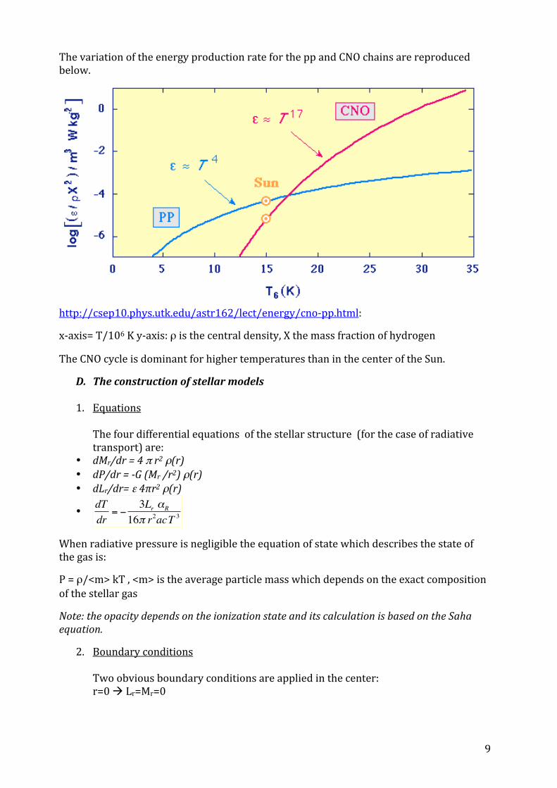
εPP ∝ X2ρ Tß ß is of the order of 4 for the pp chain and 17 for the CNO cycle

9

The variation of the energy production rate for the pp and CNO chains are reproduced below.

http://csep10.phys.utk.edu/astr162/lect/energy/cno-‐pp.html:

x-‐axis= T/106 K y-‐axis: ρ is the central density, X the mass fraction of hydrogen

The CNO cycle is dominant for higher temperatures than in the center of the Sun.

D. The construction of stellar models

1. Equations The four differential equations of the stellar structure (for the case of radiative transport) are:

• dMr/dr = 4 π r2 ρ(r) • dP/dr = -‐G (Mr /r2) ρ(r) • dLr/dr= ε 4πr2 ρ(r)

•

€

dTdr

= −3Lr αR

16π r2acT 3

When radiative pressure is negligible the equation of state which describes the state of the gas is:

P = ρ/<m> kT , <m> is the average particle mass which depends on the exact composition of the stellar gas

Note: the opacity depends on the ionization state and its calculation is based on the Saha equation.

2. Boundary conditions Two obvious boundary conditions are applied in the center: r=0 à Lr=Mr=0

10

At the surface of the star, pressure and temperature are much smaller than in the center r=R à Tr=0, Pr =0 and Mr=M

3. Standard solar model The structure of the Sun is well understood. The nuclear reactions were proved with neutrino studies. The central temperature is 16 million K. The average density of the sun is only slightly higher than water. The radiation transfer is both radiative (inner part) and convective (external shell)

• Core o radius = 0 to 200,000 km o Temperature(inner radius) = 15,000,000 K o Energy generated by nuclear fusion

• Radiation Zone o radius = 200,000 to 496,000 km o Temperature(inner radius) = 7,000,000 K o Energy transported by electromagnetic radiation

• Convection Zone o radius = 496,000 to 696,000 km o Temperature(inner radius) = 2,000,000 K o Energy transported by convection

From H. Bradt, Astrophysics Processes, Figure 4.5

11

E. Scaling laws along the Main Sequence

Dimensional approximations applied to the equation of stellar structure can be used to give rough estimates of the main parameters

ρ~M/R3

dP/dr = -‐G (Mr /r2) ρ(r)

dP/dr~-‐Pc/R (P~0 at the surface of the star).

This yields Pc~-‐GM/R (M/R3)∝M2/R4à P∝M2/R4

From the equation of state P = ρ/<m> kT : Tc~(GM2/R4) (<m>/k) (R3/M) and Tc∝M/R

Then L=4 π σ R2 T4 ∝R2M4/R4= M4/R2

dLr/dr= ε 4πr2 ρ(r) and εPP ∝ X2ρ Tß

dLr/dr~L/R gives L∝R3 (M/R3)2 Tß∝ Mß+2/Rß+3

Combining the two expressions of L:

€

L∝M2β+8β+1

For ß=4 it leads to L∝M3.2

Note: Alternatively from the equation of radiative transfer:

dT/dr =-‐3 L/(16 π r2). χρ/(ac T3)

One gets T/R ∝ L/R2 (M/R3) (1/T3) à L∝ (TR)4/M à L∝ M3 not very different from the previous one

Exercice: page 75Choudhuri, Maoz page 47 L versus T, age versus M

Mass and luminosity of nearby, binary stars can de determined.

The graph shows the results for the sun (red circle) and 121 binary stars. The line is the best fit relation corresponding to an exponent 3.9

http://www.astronomy.ohio-‐state.edu/~pogge/Ast162/Unit2/structure.html

12

F. Stellar evolution

As mentioned above combining the fundamental equations with the equations of state for a perfect gas and the Saha equation for the ionized medium and boundary conditions allow to build theoretical models of stars.

1. Hertsprung-‐Russell diagram

Stars can be plotted on a diagram with the logarithm of their luminosity (L) versus the logarithm of their temperature (T) as already shown in the previous chapter (L = 4 π R2 σ T4)

In practice we use observational quantities scaling as L and T. The temperature is also a proxy of the spectral type of a star.

The X-‐axis is most of the time a color magnitude, B-‐V, i.e the difference between the apparent B (blue) and V (visual or yellow) magnitude. It is also called color index (cf chapter 1). Assuming that the stellar emission is that of a black body of temperature T, hotter stars have smaller values of B-‐V . By convention, B-‐V decreases and log(T) increases to the left of the plot.

The Y-‐axis is usually an absolute magnitude (mostly in the V band), it scales as the inverse of the luminosity of the star. Absolute magnitude decreases and luminosity increases upward. Both the flux and the distance of the star have to be measured.

As shown earlier, luminosity and temperature are fundamental quantities for stars. They occupy a reduced area in the H-‐R diagram. Most of them are lying on the diagonal region thus called the Main Sequence (MS). The Sun is lying on the MS.

The H-‐R diagram is an evolutionary diagram, stars move in different regions during their lifetime and the relative number of stars in the different ‘branches’ are dictated by the time stars spend on each of them.

The MS corresponds to hydrogen burning in the core of the stars, the luminous hot stars (upper left) are the most massive (scaling law) and the largest (cf chapter 3). The low luminosity colder stars are the least massive. We refer to chapter 3 for the discussion of the size of the stars. Stars of constant radius are distributed along diagonals roughly parallel to the MS. The giant branch is represented on the figure below.

For a given temperature the star can belong to different branches and have different luminosities (and size). The spectra of stars (giving the spectral type) are also divided in

13

luminosity classes (main sequence or dwarfs (V), subgiants (IV), giants (III), bright giants (II) and supergiants (I)). The sun is a G2 V star.

On the right side diagram, the different luminosity classes are shown

The X-‐axis is the B-‐V colour index used as a measure of the temperature, the absolute magnitude is plotted on the Y-‐axis

Starting with the scaling laws:

Tc∝M/R, ρ~M/R3 and P∝M2/R4,

A giant star with the same temperature as a MS star (along a vertical in the H-‐R diagram) will have a lower density and pressure, its spectrum will reflect this as we will see later, therefore the luminosity classes correspond to specific spectral signatures.

The right side plot is an example of HR diagram for nearby stars with the main branches. It is the H-‐R colour-‐magnitude diagram of 16631 stars observed by the Hipparcos satellite. The large overdensity of the main sequence branch is due to the long time stars spent on this branch. The other overdensity in the giant branch correspond to the horizontal branch, which is also a stable, long phase of stellar life.

14

2. Evolution of single stars

Stars form from the molecular gas of the interstellar medium. They first collapse to densities at which nuclear burning of the hydrogen can start, the star starts its life on the Main Sequence.

a. Lifetime on the Main Sequence

A star spends most of its life on the MS. Once again dimensional approximations can be used to roughly estimate this duration

L ∝ E/tSP , where E is the energy emitted and tSP the time spent on the MS

L ∝ M/tSP since the energy emitted comes from nuclear reactions (E∝ M c2)

The lifetime of sun-‐like stars on the MS is ~1010 years, it is halfway through its main sequence lifetime.

tSP = 1010 (M/Msun) /(L/Lsun)

L scales approximately as M3,

tSP = 1010 (M/Msun)-‐2

The life of massive stars (106-‐107 years for > 10 Msun stars) is short compared to the age of the sun. The observation of such stars means that star formation is an on-‐going process in the Milky Way.

Stars less massive than the sun have ages close to that of the Universe (~14 Gyr)

b. Very brief description of the post main sequence evolution

• All through the main sequence stage, the compression of gravity is balanced by the outward pressure from the nuclear fusion reactions in the core. Eventually the hydrogen in the core is all converted to helium and the nuclear reactions stop.

• Gravity takes over and the core shrinks. The layers outside the core collapse too, the ones closer to the centre collapse quicker than the ones near the surface. As the layers collapses, the gas compresses and heats up. Eventually, the shell layer just outside the core gets hot and dense enough for fusion to start. The fusion in the layer just outside the core is called shell burning. This fusion is very rapid because the shell layer is still compressing and increasing in temperature, the mass of the helium core increases.

• The luminosity of the star increases from its main sequence value. The gas envelope surrounding the core puffs outward under the action of the extra outward pressure. As the star begins to expand it becomes a sub-‐giant and then a red giant. The most massive stars will become highly luminous super-‐giants.

• The contraction of the core is stopped when it becomes dense and hot enough to burn the helium. It yields heavier elements as carbon, oxygen and neon together with nuclear energy. Helium is burning in the core and hydrogen burning occurs in a shell outside the helium core. In low mass stars (like the Sun), the onset of helium fusion in the core can be very rapid, producing a burst of energy called a helium flash. Massive stars do not experience this flash.

• During their giant phases the stars eject large amounts of mass by means of stellar winds, these ejecta enrich the interstellar medium with elements heavier than

15

hydrogen and helium • Eventually the helium is depleted and continues to burn only in a shell around the

inert core of carbon and oxygen, hydrogen burning is still taking place at the outer edge

c. Last stages of the evolution Stars with an initial mass less than 8 Msun will then eject their diffuse envelope becoming a planetary nebula, the core shrinks and becomes a white dwarf. It is the destiny of the sun. Stars more massive than ~12 Msun provide sufficient temperature and pressure to initiate the burning of the carbon-‐oxygen core. The burning eventually led to an iron core, iron being the most stable nucleus, fusion will not lead to energy release. Indeed, for elements lighter than iron, nuclear fusion releases energy, for iron and all heavier elements nuclear fusion consumes energy, it is called the iron peak. Chemical elements lighter than iron (including iron) are produced by stellar nucleosynthesis, they are called primary elements. Gravity shrinks the core to such densities that iron is photo-‐desintegrated. The core collapses, a neutron star or a black hole is created and the envelope is ejected. Elements heavier than iron are created in the shock wave by a rapid capture of neutrons (r-‐process). These neutron rich nuclei are unstable and evolve in more stable nuclei with higher atomic number and same atomic mass. All the elements are dispersed in the interstellar medium. It is the supernova explosion. The cores of the more massive stars (> ~25 Msun)may collapse directly in a black hole and produce a gamma ray burst. However it strongly depends on the mass loss of these stars prior to the collapse and their evolution remains uncertain. Gamma-‐ray bursts were discovered 50 years ago. They occur about once per day on the sky. Their cosmological origin is now proved. They are so intense that they can be observed in the first giga year after the Big Bang. Their nature is still debated (supernova explosion, coalescence of two neutron stars into a black hole…) http://skyserver.sdss.org/dr1/en/astro/stars/stars.asp : evolution of a sun-‐like star

16

Some main sequence lifetimes for different stellar masses

25.0 Msun: 4 million years 15.0 Msun : 10-‐15 million years 5.0 Msun : 65 million years 3.0 Msun: 800 million years 2.25 Msun : 480 million years 1.5 Msun: 4.5 billionn years 1.00 Msun: 7-‐10 billion years 0.5 Msun: 25 billion years 0.10 Msun: 100 billion years

3. HR diagram and stellar evolution in clusters

a. Globular clusters

Globular clusters are tightly bound clusters of typically ~106 stars. These stars are old and they were formed in the early stages of the Galaxy (Milky Way) formation. They contain no gas and no new star. All the stars are mostly of the same age and have evolved in an unperturbed environment. It is a relatively simple case of a coeval population and its evolutionary state can be studied with their H-‐R diagram.

17

In the H-‐R diagram of the globular cluster M3 (Messier 3) the high mass stars in the upper part of the Main Sequence are missing. The lifetime of these stars is short compared to the age of the cluster. These stars have moved on the giant branch and the most massive ones collapsed in black holes, neutron stars and white dwarfs. The end of the Main Sequence is called the turn off point. A relatively large number of stars populate the so-‐called horizontal branch. These stars burn helium in their core in a stable way. The stars are initially more massive than the sun. The position of the turn off gives the age of the cluster, 10 Gyr for M3, the corresponding isochrone is plotted on the H-‐R diagram of M3.

b. Open clusters

Star birth occurs in clusters which originate from the fragmentation of molecular clouds. Typically these clusters are less massive than the globular clusters and are not gravitationally bound. Eventually they will disperse. The clusters visible today contain coeval populations of stars, younger than the ones present in the globular clusters. The interpretation of the H-‐R diagram of an open cluster is the same as for the globular clusters: the most massive stars evolved off the main sequence and the turn off point gives the age of the cluster. The main branches of the most popular clusters are plotted on the plot below, the ages at which stars leave the main sequence are indicated in red.

18

Appendix: Evolutionnary tracks for models of stars after the Main Sequence (from Iben, 1967 Annual review of Astronomy and Astrophysics, vol. 5, page 571 Model mass is shown next to the initial point (corresponding to zero age main sequence). Elapsed time between points are shown in the table below

Numbers in parentheses are powers of 10 by which entries are multiplied

References Astrophysics , decoding the cosmos, Irwin, Wiley Astrophysics in a nutshell, Maoz, Princeton University Press Astrophysical processes, Bradt, Cambridge University

19

Quiz to test your knowledge: if you cannot answer to these questions you must go back to your course before coming to the tutoring lecture related to this chapter. WARNING: answering to these questions does not mean that you know all you need to know about the chapter…. 1. Write the basic equations of the stellar structure: -‐mass continuity –hydrostatic

equilibrium-‐energy transport 2. What is the virial theorem? 3. Give the mass relation luminosity for stars (approximate law) 4. Relate the lifetime of a star on the main sequence to the solar mass and

luminosity 5. Explain how to interpret the HR diagram of stellar clusters

20

Chapter 5

The interstellar medium, interaction of light with matter

The medium between the stars is essentially empty: in the solar neighbourhood stellar density is 6 10-‐2 pc-‐3. The interstellar medium (ISM) is filled with a tenuous hydrogen and helium gas and a very small contribution of heavier atoms. These elements are either in atomic, molecular or ionized forms at various temperatures. Dust grains contain a large fraction of these heavier elements. These grains are mostly formed in the circumstellar environment of stars at the end of their life. Gas and dust are heated by photons emitted by stars. Interstellar grains absorb a large fraction of the photons emitted by stars and re-‐emitted corresponding energy thermally as mid-‐ and far-‐infrared photons (>5 µm). Molecules form on the surface of interstellar grains, in particular the most abundant hydrogen molecule H2. In this chapter we will introduce some major phases of the ISM, without any attempt to be exhaustive:

• Ionized gas. We will describe HII regions (even if a large fraction of the ionized gas does not reside in distinct HII regions): these nebulae of ionized gas are sometimes spectacular like the Orion nebula. The temperature of these regions is of the order of 104 K and densities range from 10 (diffuse regions) to 103-‐104 cm-‐3 (dense regions). The spectra of these regions are dominated by H and He recombination lines and collisionally excited, forbidden line emission from ions ([OII], [OIII], and [NII]). HII regions are also sources of thermal radio emission (free–free) from the ionized gas and of infrared emission due to warm dust. HII regions are formed by young massive stars with spectral type earlier than about B1 (Teff > 25 000 K), which emit photons beyond the Lyman limit (hν> 13.6 eV) and ionize and heat their surroundings.

• Neutral gas, atomic and molecular. We will focus on the cold diffuse HI clouds revealed by the 21 cm line of the atomic hydrogen (~100 K, ~50 cm-‐3) and on molecular clouds (~10 K, ~200 cm-‐3 in average) observed in the CO J=1-‐0 transition at 2.6 mm.

• Interstellar dust. The size of dust grains varies from nm to µm. Dust represents only ~1% of the mass of the interstellar medium but plays a large role in the physics and chemistry of the ISM. We mention here only some processes. Dust absorbs and scatters stellar light. The energy absorbed by dust grains heats them and is re-‐emitted in the mid-‐ and far-‐infrared. Almost half of all the energy emitted by stars in the Galaxy in the ultraviolet and visible is absorbed by dust, then re-‐emitted at much longer wavelengths. Dust grains also act as catalysts : the H2 molecule can also form on dust grains.

Before describing these different components we will present some elements of radiation transfer in different media.

21

I. Basics of radiation transfer theory

The light we see with our telescopes is a tiny fraction to what was generated. With no intervening matter the energy detected is only diminished by distance. With intervening matter, energy is transferred or shared. The radiation that is emitted in one region can be absorbed by other matter, which can thus be radiatively heated. In this way radiation can act a carrier of energy exchange between matter parcels that are otherwise too far apart to interact with each other. In other words: radiation is not only a diagnostic tool for us as astronomers, it is also (and perhaps even predominantly) a critical ingredient in the thermal balance of the objects we observe. A serious interpretation of observations therefore often forces us to learn about the emission, absorption and transport of radiation inside our objects of interest. We can also learn about the material within which energy transport is occurring. The theory of “radiative transfer” (also called “radiation transport”) is the theory of how radiation and matter interact.

A. Radiative transfer equation

1. Specific intensity

This quantity was already introduced in the previous chapters to describe stellar radiation. Let us consider radiation as a movement of photons along straight lines. In empty space photons do not encounter any obstacle and photons do not interact. So if we wish to measure the amount of radiation at some point r in space, we also have to specify in which direction we are “looking”. We already defined the specific intensity : it is the radiative energy per unit time per unit solid angle and per unit frequency (or wavelength) passing trough a unit area that is perpendicular to the direction of emission. It is usually called Iν.

Iν has units W m-‐2 Hz-‐1 sr-‐1 (or erg cm-‐2 s-‐1 Hz-‐1 sr-‐1). The formal definition of the specific intensity is

€

dE = Iνdν dAcos(θ) dΩ dt dE is the energy (erg or J) passing through dA The geometry is shown: dA cos(θ) is the projected area perpendicular to the direction we are looking.

a. Formal radiative transfer equation

Let us consider an incoming signal passing through a cloud (i.e a region with interstellar matter)

Iν Iν +d Iν

dr

22

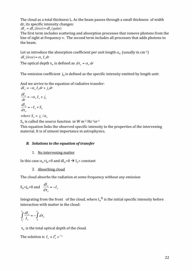
The cloud as a total thickness L. As the beam passes through a small thickness of width dr, its specific intensity changes:

€

dIν = dIν (loss)+ dIν (gain) The first term includes scattering and absorption processes that remove photons from the line of sight at frequency ν. The second term includes all processes that adds photons to the beam. Let us introduce the absorption coefficient per unit length αν (usually in cm-‐1)

€

dIν (loss) = αν Iνdr The optical depth τν is defined as

€

dτν = αν dr

The emission coefficient jν is defined as the specific intensity emitted by length unit: And we arrive to the equation of radiative transfer:

€

dIν = −αν Iνdr + jνdrdIνdr

= −αν Iν + jν

dIνdτν

= −Iν + Sν

where Sν = jν /αν

Sν is called the source function in W m-‐2 Hz-‐1sr-‐1 This equation links the observed specific intensity to the properties of the intervening material. It is of utmost importance in astrophysics.

B. Solutions to the equation of transfer 1. No intervening matter

In this case αν=jν=0 and dIν=0 à Iν= constant

2. Absorbing cloud

The cloud absorbs the radiation at some frequency without any emission

Sν=jν=0 and

€

dIνdτν

= −Iν

Integrating from the front of the cloud, where Iν0 is the initial specific intensity before interaction with matter in the cloud:

€

dIνIνIν

0

Iν

∫ = − dτν0

τν

∫

τν is the total optical depth of the cloud.

The solution is

€

Iν = Iν0 e−τν

23

The intensity diminishes exponentially with the optical depth. We will see below that this equation is used to describe the extinction of optical light in a dusty medium.

3. Emitting cloud

αν=0 and

€

dIνdr

= jν

Assuming that the emissive properties do not change along the line of sight (is independent of r), the solution is :

€

Iν = Iν0 + jν × r

4. Cloud in thermodynamic equilibrium

In thermodynamical equilibrium (TE) inside the cloud, the temperature is constant and the specific intensity is given by the Planck function Bν everywhere in the cloud.

The second relation is known as Kirchoff’s law and describes the thermodynamic equilibrium.

This case is not very realistic, a notable exception being the cosmic background radiation.

5. Emitting and absorbing cloud in local thermodynamic equilibrium

We must define the concept of LTE: local thermodynamic equilibrium. In this case, the matter has the properties of the TE but only locally. A good example is the interiors of stars. The densities are high enough for the radiation and matter to be trapped together locally and to be in equilibrium. One can define cells inside which the TE is verified but there is a global gradient of temperature from a cell to another one. In other words the TE is verified at some relevant size scale.

In case of LTE, the source function is the Planck function and there is a net flux of radiation through the cloud.

€

dIνdτν

= −Iν + Bν

Iν = Ae−τν + Bνif τ = 0, Iν

0 = A+BνIν = (Iν

0 − Bν )e−τν +Bν

Iν = Iν0 e−τν +Bν (1− e

−τν )

It is interesting to study specific circumstances:

• If τν>>1, the medium is called optically thick and Iν=Bν, we find again the thermodynamic equilibrium

• If τν<<1, the medium is called optically thin and

€

Iν ≈I ν0 (1− τν )+ Bν τν

€

0 = −αν Bν + jνand Bν = jν /αν = Sν

24

In a more general case Bν is replaced by the source function Sν

The observed intensity depends on the temperature and density of the foreground cloud

6. Emission and absorption lines

We have seen that the spectra of stars exhibit absorption lines, we will see in the next sections that emission lines are common in the spectrum of the interstellar medium.

Here we explain what are the conditions for a line to be seen in absorption or in emission:

We assume the simple case of a foreground cloud and a background source, forming a spectral line at a given frequency. We also assume that the transmission is perfect at all frequencies of the line.

€

Iν =I ν0 e−τν +Bν (1− e

−τν ) if Iν <Iν0 there is an absorption line, if Iν >Iν0, there is an emission line.

From the above equation:

€

I ν0 e−τν +Bν (1− e

−τν ) < Iν0

⇒ Iν0 > Bν

à absorption line

€

I ν0 e−τν +Bν (1− e

−τν ) > Iν0

⇒ Iν0 < Bν

à emission line

In other words if the temperature of the foreground cloud is less than the brightness of the source the line is seen in absorption, as it is the case for stars.

If the medium is cold as compared to the background source and thin:

€

Iν =I ν0 (1− τν )

Iν =I ν0 (1−ανL)

if L is the total length of the foreground cloud

The observed specific intensity gives information on the amount of matter in the foreground cloud (see problems)

If the temperature of the foreground cloud is higher than the brightness of the source the line is seen in emission. If there is no background source (Iν0=0) the line is always seen in emission (it will be the case for HI clouds).

25

II. Dust component: absorption and emission

Everywhere in the sky there is some evidence for dust. Dark bands are clearly visible in the Milky Way for example and any image taken with a filter in optical of nearby spiral galaxies exhibits some dark lanes due to dust obscuration.

A. General concepts

The decrease in the luminosity of a star when it is seen through a dust cloud is due to two different physical phenomena: the absorption of photons by the dust grains and the scattering of photons in directions other than the incident direction. The ensemble of these phenomena is called extinction. Extinction depends upon the grain composition, shape and size distribution and also upon the wavelength. The extinction A(λ) is expressed as the ratio of the emerging flux I(λ) and the incident flux I0 (λ):

€

A(λ)=− 2.5 log I(λ)I0(λ)⎛

⎝ ⎜

⎞

⎠ ⎟

Introducing the optical depth:

€

I(λ)=I0 (λ)e−τλ

One deduces

€

τλ =0.921A(λ)

The extinction curve or extinction law gives the variation of the extinction with wavelength (or the inverse of the wavelength). It is obtained by comparing the light of 2 stars assumed to be identical (same spectral type and class of luminosity) but seen along a different line of sight, i.e. a different amount of intervening matter. The stars are chosen to exhibit very different extinctions. Note that the measure of the absolute extinction is very difficult since stars are not sufficiently known for such a measure. Only the relative extinction curve is derived.

Usually the extinction curve is normalized to the difference of extinction in the B and V broad bands. This quantity is called colour excess:

EB-‐V = AB –AV and the extinction curve is given as A(λ)/EB-‐V, other normalisations like A(λ)/AV are also used.

The quantity AV/EB-‐V = RV is called the selective extinction. The average extinction curve for the Milky Way is given below. The average value of the selective extinction RV is found equal to 3.05 +\-‐ 0.15

The shape of the extinction curve and the value of the selective extinction are known to vary substantially along different directions. It is attributed to variations of grain properties.

26

Eλ-‐V= A(λ)-‐AV. The inverse of the wavelength is plotted on the x-‐axis, in the optical (where

the B and V bands lie) a rough approximation gives Eλ-‐V∝ 1/λ.

The extinction curve provides clues about the composition of the dust. The changes in slope as well as the obvious peak at 4.6 µm-‐1 (217.5 nm) can be compared to laboratory spectra to determine the material responsible. For the peak at 217.5 nm the best candidate is graphite or related particles.

Practically it is difficult to find a unique solution for the dust composition with the extinction curve only.

B. Composition of dust:

The size of grains is distributed along a continuum: Large grains are of the order of 0.1 µm in size, and very small grains of order of 0.01 µm.

A size distribution is commonly used since it works well to describe the dust characteristics: for a specie i the number of grains with size comprised between a and a+da is :

dni = Ai nH a-‐3.5 da amin<a<amax (amin≈0.05 µm, amax≈0.25 µm)

nH is the density of hydrogen nuclei, taken as a reference for abundance.

Carbons et silicates are assumed to be the main components of interstellar dust. Carbon easily form hydrogenated rings called Polycyclic Aromatic Hydrocarbons (PAHs). Their signature is found in the mid-‐IR spectra of the ISM (5-‐20 µm). Some examples of PAHs are given here

27

Whittet 2003: the total extinction curve predicted by the model fits very well the black points and solid curve. It is the sum of contributions from large composite grains of carbon and silicate (dot dashed curve), from small graphite grains (dashed curve) and from PAHs (dotted curve).

C. Optical depth and opacity of dust

We already introduced the optical depth, as a unitless parameter defined as

€

dτν =αν dr where αν is the absorption coefficient (cm-‐1) at a given frequency.

The infinitesimal variation of the optical depth is also given by

€

dτν =αν dr=σν ndr

where σν is the effective cross-‐section (cm2), n the density of particules (cm-‐3).

The total optical depth over the total line of sight through the source is given by:

€

τν =0

l

∫ σν ndr≈σν n l , where l is the total line of sight thickness of the medium (assuming

that the cross-‐section and the density are constant in the cloud)

Important Note: the optical depth provides a quantitative description of the opacity of a medium since it is related to the mean free path of the photons:

The mean free path is determined by considering a small cylinder with a volume V = π R2 l with a particule density n, an effective cross-‐section of the particules, σ. The probability that a photon will encounter a particule is Nσ/π R2 where N= n V is the total number of particules.

28

Illustration from J. Irwin, decoding the cosmos, Wiley

If we ensure that an interaction will occur:

1= nVσ/πR2 = nσl and the mean free path is given by l = 1/nσ

• if the optical depth is lower than 1, the medium is described as ‘optically thin’, the probability that a photon is absorbed or scattered is lower than 1

• if the optical depth is larger than 1, the medium is described as “optically thick” and the probability that a photon is absorbed or scattered even several times is very high

• if τν =1 the line of sight thickness is equal to the mean free path and the medium is just “optically thick”

The interaction of light with dust is difficult to model. The dust grains have irregular shapes, they span a range of size, have different composition etc…

A popular, simple modelling is the Mie theory which assumes that the grains are spherical. . The interaction is characterized by the extinction efficiency factor Qext(λ) as a function of x= 2πa/λ, a is the grain radius and λ the wavelength of the light.

Qext(λ) is the ratio between the effective cross-‐section of the grain to its geometric cross-‐section.

The optical depth is:

τ(λ) = n σ l = n Qext(λ) π a2 l

Efficiencies are defined for the scattering and absorption processes separately:

Qext=Qabs+Qsca

The albedo is the ratio between the scattering and extinction cross-‐section or equivalently (for the Mie theory) between Qsca and Qext

29

From Whittet, dust in the galactic environment, IoP

Absorption, scattering and extinction efficiency factors as a function of x=2πλ/a for a weakly absorbing grain. Peaks arise in the scattering component of Qext caused by resonances between wavelength and grain size and these will disappear when the contributions of grains with many different radii in a size distribution are summed

D. Interstellar dust emission

Interstellar grains are in general heated by the absorption of UV and visible radiation from stars. The balance of the energy absorbed by dust must re-‐emerge in the infrared. In typical regions, a steady state is reached and dust grains are heated at a temperature Td and re-‐emit the power they absorb. Typical values for Td are 10-‐20 K (for large grains (0.1 µm) and low density media). Their emission is expected in the infrared (according to the Wien law, dust emission is close to that of a black body as described below). Dust emission accounts for ~30% of the total emission of the Milky Way and can amount to nearly 100% in infrared luminous galaxies.

We first consider a perfect spherical large dust grain (radius a~0.1 µm), from the calculations in chapter 3 the power absorbed by the grain of efficiency factor Qabs and radius a is :

Labs = π a2 ∫ Qabs (λ) c uλ dλ= π a2 ∫ Qabs (λ) 4π Bλ dλ Bλ is the specific intensity of the interstellar radiation field. (Note that the calculations in chapter 3 are with respect to frequency and not to wavelength)

The grain emits a power:

Lem = 4 π a2 ∫ Qem (λ) π Bλ (Td) dλ

30

From Kirchoff’s law Qabs(λ) = Qem(λ), Qem(λ) is usually called the emissivity, Bλ (Td) is the Planck function. Q(λ) can be calculated, for instance with the Mie theory.

Most of the emission occurs and the far-‐infrared (FIR, λ> 30 µm) but begins in the mid-‐IR (λ> 5 µm) [the reader can check the corresponding temperature of the grain if a perfect Black Body emission is assumed] and QFIR(λ) ∝λ-‐ß, ß depends on the nature of the grain and is comprised between 1 and 2.

Note that the above calculations are based on a thermal equilibrium which is not satisfied for very small grains (a<~0.01 µm) whose temperature can fluctuate a lot. The mean temperature of these small grains is larger than that of large grains

Emission features centered at 3.3, 6.2, 7.7, 8.6 and 11.3 µm are clearly detected in the spectra of a wide variety of interstellar medium and in the global spectrum of external galaxies. These features are assigned to vibrational modes of the class of molecules called Polycyclic aromatic hydrocarbures (PAHs). It was confirmed by laboratory measurements. As mentioned above a large variety of PAHs is expected to be present in the ISM.

From Whittet, dust in the galactic environment, IoP:

observed and laboratory wavelengths of the principal features assigned to PAHs and the global spectrum of diffuse regions of the interstellar medium

31

III. Gas component

A. Ionized regions

1. Definition

Ionized atomic hydrogen regions, termed “HII Regions”, are composed of gas ionized by photons with energies above the hydrogen ionization energy of 13.6 eV (also called Lyman limit). “Classical HII Regions” are ionized by hot O or B stars (or clusters of such stars) and are associated with regions of recent massive-‐star formation. The ejected outer envelopes of hot remnant stellar cores are called « Planetary nebulae ». The physical origins of these types of gaseous nebulae are very different but the physics governing them is basically the same. In this course we refer to the classical HII regions ionized by young, massive stars. The UV, visible and IR spectra of HII regions are very rich in emission lines, collisionally excited lines of metal ions and recombination lines of Hydrogen and Helium. HII regions are also observed at radio wavelengths, emitting radio free-‐free emission from thermalized electrons and radio recombination lines from highly excited states of H, He, and some metals. At frequencies ν higher than ν0 = 13.6 eV, the absorption cross-‐section can be

approximated by:

€

σν ≈σ 0ν0ν

⎛

⎝ ⎜

⎞

⎠ ⎟ 3

Where σ0 is the absorption cross-‐section at the Lyman limit: σ0=6.3 10-‐18 cm-‐3

The typical optical depth of Lyman limit photons in an HII region is

τ = σ0 nH l, nH is the HI gas surface density,

in the mid-‐plane of the Milky Way nH ≈ 0.6 cm-‐3

An optical depth of unity corresponds to 0.09 pc, photons of higher energy can travel over larger distances before being absorbed (but less than 1 pc for most of the ionizing photons).

2. Size of HII regions

Let us consider a spherical region of constant density n. At a distance R of a star with an ionizing flux all the hydrogen is ionized. If the star produces dN ionizing photons per second, the radius of the region grows by dR where:

dN/dt = 4 π R2 n (dR/dt)

Ions and electrons recombine in the sphere at a rate α

dN/dt – (4/3 π R3) ne ni αrec = 4 π R2 n (dR/dt)

ne=ni=n (ne and ni are the electron an ion density respectively)

When ionization and recombination are at equilibrium dR/dt = 0, the radius is called RS (Stromgren sphere and radius):

32

dN/dt = Sion and

€

Rs =3Sion

4π n2αrec

⎛

⎝ ⎜

⎞

⎠ ⎟

1/ 3

It is the case of an ionization bounded HII region

From Osterbrock and Ferland: Astrophysics of gaseous nebulae and active galactic nuclei, 2006. Ne and Np are the electron and ion densities, the calculation is performed under case B of recombination (see below)

3. Recombination rates and lines

The recombination rates are calculated under specific assumptions. The recombination rate into each atomic state is calculated and all the recombination rates are summed to get the total αrec it is know as the case A recombination rate coefficient.

In galactic HII regions the gas is optically thick in the Lyman lines (recombination on the n=1 state) and the photons of the Lyman series are immediately re-‐absorbed by the gas. The recombination rate coefficient is thus calculated by excluding all the recombinations into the n=1 state, this case is called case B.

The most intense recombination line in an HII region is the Hα line at 656.3 nm, giving their characteristic red colour to these regions.

The radio recombination lines correspond to transitions between levels with very high quantum numbers (> ~30).

http://burro.astr.cwru.edu/Academics/Astr221/Light/spectra.html, energy diagram for the hydrogen atoms and the 3 first series (Lyman, Balmer, Paschen)

Osterbrock

33

3. Forbidden metal lines

In the gas at very low density, metastable energy levels of atoms and ions can be populated (they are de-‐excited by collisions in high density media), the decay is only possible through forbidden transitions not seen on earth. It is for example the case of the oxygen lines [OII] at 372,7 nm [OIII] at 495,9 and 500,7 nm which are commonly observed in HII regions.

B. Neutral regions

1. HI content, the 21 cm line of neutral hydrogen

Neutral regions have their hydrogen particles in the ground state. Hydrogen atom has a nuclear spin which is coupled to the angular momentum of the electron to form the total momentum F. This coupling is only important in the ground state when the electron is close to the nucleus. It results in an hyperfine splitting of the ground state: either the proton and electron spinning in the same sense (F =1), or the proton and electron spinning in opposite sense (F =0), the former orientation having the higher energy. The statistical weights of these two states are given by g = 2F + 1. Hence the spin-‐parallel state has a statistical weight of g2 = 3 and the spin-‐anti-‐parallel state has a statistical weight of g1 =1, where the subscripts, 2, and 1 refer to the upper and lower energy levels, respectively.

The 21 cm transition is sometimes called the spin-‐flip transition since de-‐excitation involves this process. The transition from F =1 to F = 0 is a forbidden transition.

The spontaneous emission probability is 2.87 10-‐15 s-‐1 and the radiative lifetime of the upper level is of the order of 107 years. The sub levels are in collisional equilibrium and thus at local thermal equilibrium. De-‐excitation by collisions substancially reduces the lifetime of the upper level

34

Since there is so much atomic hydrogen in space, it is possible to observe the resulting spectral line, the 21 cm line of hydrogen. Since the Local Thermal Equilibrium (LTE) applies for this line

€

Iν = Iν0 e−τν +Bν (1− e

−τν ) At low frequency the Planck function can be approximated (chapter 3)

€

Bν =2hν 3

c21

e(hν /kT ) −1≈2hν 3

c21

hν /kT≈2kν 2

c2T

The same formalism is applied to Iν even if it is not a Black Body emission. This is the definition of brightness temperature which is extended to include any astrophysical source, whether or not its emission approximates that of a black body. In this case the brightness temperature varies with the frequency

€

Tν = Tν0 e−τν +T (1− e−τν ) in the general case

Without a background source (i.e with only an HI cloud emitting at 21 cm)

€

Tν = T (1− e−τν )

The HI cloud are optically thin

€

Tν ≈ T τν T is the kinetic temperature of the gas

€

τν =σν n1l∫ dl =1/4σν nHI

l∫ dl =1/4σνNHI

σν is the effective cross section, n1 the number density of the lower level of the ground state (with statistical weight equal to ¼) and NHI the column density (cm-‐2) of H atoms.

Note: σν is proportional to 1/T and the line intensity does not depend on the temperature of the gas but only on NHI

2. Molecular clouds

In molecules, there are two specific types of transitions that can occur: rotational and vibrational transitions. Considering di-‐atomic molecules, if the two nuclei are different, then the molecule will have a permanent electric dipole. For example, in the CO molecule, the oxygen atom has a slight negative charge and the carbon atom has a slight positive charge. A radiation is emitted when a transition occurs from one rotational state to another. It is nevertheless necessary for an electric dipole to be present in order for a rotational change to produce a rotational spectral line. Rotational transitions correspond to the smallest energy changes in molecules and the lines have low frequencies (in the far-‐IR or mm part of the spectrum)

35

H2 molecules do not have electric dipole moments and they display no rotationally-‐induced electric dipole radiation. The much weaker quadrupole transitions require relatively high energy to excite which are not easily found in the interstellar medium. Therefore the most abundant molecule which trace the whole molecular content of the clouds cannot be observed directly. The alternative is to consider the next most abundant molecule, which is carbon monoxide. The CO(J=1-‐0) line at 2.6 mm is mostly observed. This rotational CO line is collisionally excited, and the species with which it collides will be the most abundant molecule, H2. The line is a strong line, is easily observed, and in fact, is often optically thick. Other CO lines may also be present, depending on excitation conditions (for example, there are lines at 1.3 mm, and 0.87 mm), and lines of the C18O and 13CO isotopes, which are weaker and optically thin, may also be observable. Therefore, a variety of CO lines provide important diagnostics of interstellar molecular clouds. References Astrophysics, decoding the cosmos, Irwin, Wiley The interstellar medium, Lequeux, Springer Dust in the galactic environment, Whittet, 2nd edition, IoP, series in Astronomy and Astrophysics

Quiz to test your knowledge: if you cannot answer to these questions you must go back to your course before coming to the tutoring lecture related to this chapter. WARNING: answering to these questions does not mean that you know all you need to know about the chapter…. 1. Write the radiation transfer equation, define all the components in the more

general case and for LTE conditions 2. Give the definition of the extinction in magnitude, how is defined the color

excess? 3. What ‘optically thick’ means?` 4. Calculate the radius of the Stroemgren sphere

36

Chapter 6

An introduction to galaxies Galaxies are the building blocks of the Universe. In cosmological studies, galaxies are considered as point sources with a mass. However, galaxies are very complex systems built from many separate components: stars, gas, dust, magnetic fields, black holes…. In galaxies, gas turns into stars of different luminosities and masses. Gas and stars, distributed sometimes in very different ways are called the luminous matter to contrast with the dark matter which we know only through the pull of its gravity. Each galaxy is the result of a long story starting with the formation of the dark matter halo, followed by the formation of stars and the evolution of their shape to become the objects we are observing in the nearby universe. In this chapter we will introduce the major concepts about the physics of galaxies, without any attempt to be exhaustive. Most of the illustrations come from the volume ‘Galaxies in the universe: an introduction’, by Sparke and Gallagher, Cambridge University press. All of them are available at: http://www.astro.wisc.edu/~sparke/book/webfigs.html

A. The Milky Way Any lecture on galaxies has to begin with our own Galaxy, called the Milky Way (MW). We are inside this large spiral galaxy, we have a close view of its stellar and gas content . A schematic side view of the Milky Way is given below together with a reconstitution of its main constituents

37

The most prominent features (in terms of luminosity) are disk and the bulge. The sun lies in the stellar thin disk, which is roughly circular. The central part of the Galaxy is called bulge and it hosts a black hole (MBH~ 4 106 Msun) in its nucleus. The radius of the disk is approximately 15 kpc (the Sun is lying about 8 kpc from the Galactic center). The scale height of the (thick) disk is approximately 1 kpc. Most of the stars and all the young massive ones lie in the thin disk whose scale height is a few hundreds of parsecs, the HI and H2 gas is lying in an even thinner layer (~100 pc from the midplane). Disk and bulge are rotating, the duration of a solar orbit is ~250 Myr. Stars and clouds of the (metal-‐poor) halo do not have any organized motion. Few more numbers about the MW: Disk luminosity: 15-‐20 109 Lsun Stellar mass in the disk: 60 109 Msun Bulge luminosity: 5 109 Lsun Stellar mass in the bulge: 20 109 Msun We will see that the orbital speed of gas and stars require the total mass to be more than the one measured for stars and gas. It is called dark matter, we usually assume that it is distributed in a spherical halo. The nature of this dark matter is essentially unknown and is one of the main fields of investigation of particle and theoretical physics today. B. The galaxy menagery Soon after the confirmation of their existence in the 1920s galaxies were classified by Hubble according to their morphology observed in optical (the only wavelength range observable at that time). He recognized three main types of galaxy: ellipticals, lenticulars, and spirals, with a fourth class, the irregulars, for galaxies that would not fit into any of the other categories. This classification is still used by astronomers working in the nearby or in the distant universe even if these classes are specifically defined for nearby, very luminous, systems. The popularity of the ‘Hubble sequence’ is explained by its link to important physical properties of galaxies as we will see below.

38

A modified form of the classical Hubble classification

• Elliptical galaxies appear as elliptical concentrations of stars on the sky, they are

smooth without any feature and with almost no sign of interstellar matter. They are classified as En with n=0-‐7. n is defined as n= 10(1-‐b/a), a and b are the measured major and minor axes of the ellipse. E0 looks circular on the sky. The apparent shape of an E galaxy depends on the direction from which it is seen. Ellipticals are predominantly found in rich clusters of galaxies. The largest of them, called cD galaxies, are found in the center of clusters. These system scan be 100 times more luminous than the MW when normal ellipticals have a typical luminosities a few times that of the MW. dE and dSph correspond to faint diffuse systems (not initially found by Hubble)

• Lenticular, S0 galaxies are located between ellipticals and spirals, they ressemble Ellipticals without dust, gas and spiral arms but they share with spirals a thin, fast rotating disk. About 30% of the local galaxies are classified E/S0

• Spiral galaxies all exhibit a more or less well defined spiral pattern in the disk. Their arms are outlined by bright, young (O, B) stars. Their bulge is structurally similar to an elliptical. There are two sequences of spirals : normal (S) and barred (SB) systems. In the barred spirals the spiral pattern ends at the end of a central bar whereas in normal spirals it ends either in an inner ring or continues to the center. The sequence Saà Sd is defined by the bulge to disk ratio which decreases from Sa to Sd. The arms become more open and the fraction of gas and young stars also increases from Sa to Sd. The Milky Way is probably an Sc galaxy (or an intermediate Sbc one). At the end of the spiral sequence Sm and SBm galaxies are Magellanic spirals named after their prototype the Large Magellanic Cloud, the spiral is often reduced to a single arm. About 70% of nearby galaxies are bright or moderately bright spirals Important note: the terms “early type” and “late type” are often used to describe the sequence from S0 to Sd (early to late type). It was originally justified by the increase of the fraction of young stars along this sequence and it was thought to be related to a life cycle of galaxies. This hypothesis is now discarded but the terms “early” and “late” have survived and may be confusing.

• Galaxies which did not fit into the previous categories were put in the irregular class by Hubble. Today we use this term for small, blue (with a lot of young stars) galaxies which lack any organization. The smallest of them are dwarf irregulars. Only About 3% of local galaxies are classified irregulars C. Luminosity of galaxies and stellar light distributions

1. Total luminosities

The definition of total luminosity for a galaxy is somewhat arbitrary since they do not have sharp edge. Nearby galaxies are spatially resolved most of the time and the convention is to measure their luminosity down to a given surface brightness of the order of 26 mag arcsec-‐2 . Total magnitudes are also defined by extrapolating the light emitted using the radial profile (see next section). In the distant universe and/or surveys at large

39

wavelengths, galaxies are often detected as point sources. In this case the luminosity is easier to measure. Small, faint galaxies are much more numerous than bright galaxies. The distribution of luminosities of the galaxies (or of a sub class of galaxies) is described by the luminosity function which is the number density of galaxies with a luminosity comprised between L and L+dL. A very common functional form (for stellar light only) was first proposed by Schechter in 1976 and is now called a Schechter function:

Φ(L) = dn/dL = Φ*/L* exp(-‐L/L*) (L/L*)α n is the galaxy density, Φ et Φ* are in Mpc-‐3 L et L* are expressed either in physical units or the solar luminosities. α is named the faint end slope.

The shape of the luminosity function is described by α and L*, the relative number of faint galaxies by α. Φ* is proportional to the space density of galaxies. Φ(L)

for local field galaxies : from Tempel et al. 2011, A&A 529, A53, SDSS DR7 survey

The luminosity function in the R band of local galaxies is shown above, the magnitudes are used instead of luminosity and the h parameter depends on the adopted cosmology (h~0.7). Spirals are much more numerous than ellipticals except at the bright end of the distribution.

40

2. Stellar light distributions

The surface brightness distribution of a galaxy I(r) is the amount of light per arcsec2 on the sky at a particular radius r from the center of the galaxy (this definition assumes an axisymetric distribution of the light):

Consider a small square patch of side D that is observed from a distance d, it subtends an angle α ≈ D/d

The surface brightness is:

€

I(r)= Fα2 =

L /(4πd2 )D2 /d2

=L

4πD2

I(r) is given in mag arcsec-‐2 or in Lsun pc-‐2, contours of constant surface brightness are called isophotes. Typical values for the center of galaxies are 18 mag arcsec-‐2 in the B band. The size of the galaxies is often defined by the isophote at 25 mag arcsec-‐2

a. Ellipticals and bulges

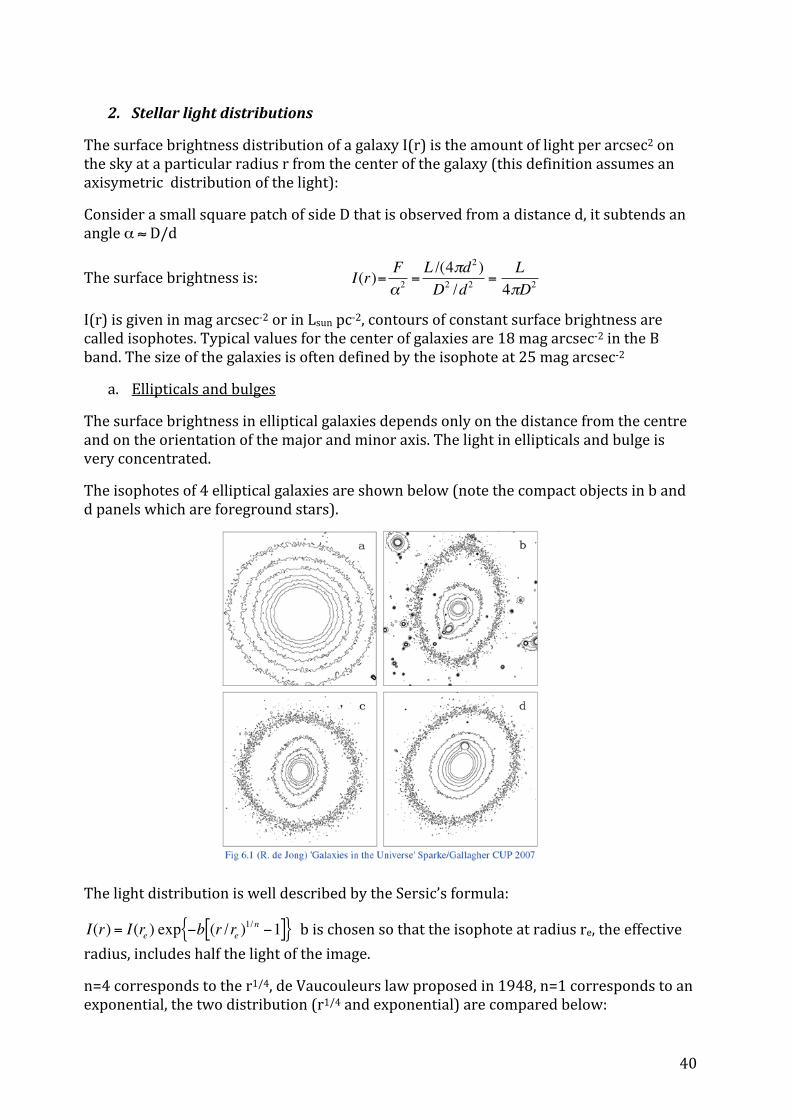
The surface brightness in elliptical galaxies depends only on the distance from the centre and on the orientation of the major and minor axis. The light in ellipticals and bulge is very concentrated.

The isophotes of 4 elliptical galaxies are shown below (note the compact objects in b and d panels which are foreground stars).

The light distribution is well described by the Sersic’s formula:

€

I(r) = I(re ) exp −b (r /re )1/n −1[ ]{ } b is chosen so that the isophote at radius re, the effective

radius, includes half the light of the image.

n=4 corresponds to the r1/4, de Vaucouleurs law proposed in 1948, n=1 corresponds to an exponential, the two distribution (r1/4 and exponential) are compared below:

41

Kormendy, in ‘secular evolution of disk galaxies’, Cambridge University Press 2013

Examples of fits with Sersic’s functions are shown above, they give excellent fits except in the internal parts which highlight the particularities of these galaxies: missing light o the right panel (M87), extra light in case of NGC 4458 and VCC 1185. A r1/4 law corresponds to a linear fit in the plots.

b. Spirals and lenticulars

They are characterized by a bright stellar disk.

42

In the above figure the isophotes of NGC7331 (left panel, adapted from Sparke & Gallagher fig 5.3), a Sb spiral, are measured on a R band image (right panel). They are almost circular near the center coming elliptical in the disk and perturbed by the spiral structure. If the disk is assumed to be circular and infinitely thin it appears as an ellipse with the axis ratio equal to cos (i) when it is seen at an angle I from face-‐on. Therefore the surface brightness can be corrected for the viewing angle: the disk is brighter by a factor 1/cos(i) than if the disk is seen face on. Then we can define a surface brightness I(r) at distance r from the center.

If we average over features like the spiral arms I(r) follows an exponential form:

€

I(r)= I(0)exp(−R /h)

The radial profile of NGC7331 is shown above (solid line), with the exponential fit (dashed line, with a scale height hR). Near the center, the contribution of the bulge put the surface brightness above the value predicted by the exponential fit.

D. Motions, masses of galaxies

Stars and gas in galaxies (i.e the baryonic matter) account for only a fraction of the mass of a galaxy and the only sure way to trace out the total mass is to study its gravitational effects. All the evidence of dark matter comes from gravitational studies at all scales. The large scale structure of the Universe is now described by modelling the gravitational effects of the dark matter alone. 1. Spirals

a. Rotation curves In spiral galaxies (including the Milky Way) the dominant motion for gas and stars is rotation, random speeds do not exceed ~10 km s-‐1. Radial velocities are determined from the measurements of Doppler shifts. Therefore they cannot be measured for face-‐on galaxies. When the viewing angle is known the rotation curve is deduced. The gas motion measurements are carried out with either the Hα line or the HI 21 cm line.

43

The figure below shows the rotation curve of several disk galaxies including that of the MW. They are all characterized by an increase of the velocity in the center and a plateau at larger distance

The constant value of the rotational speed to the observable edge of the galaxy is not explained by the distribution of the visible matter: For a circular orbit at radius r:

€

V 2 (r)r

=GM (r)r2

M(r) is the mass interior to radius r. V(r) must scale as 1/r at the edge of the galaxy, it is not observed, some matter must be added. In the center of the galaxy the bulge is dominating: taking it spherical with a constant density ρb

€

V 2 (r) =Gr43π r3ρb

V(r) scales as r in the central part of the galaxy, roughly consistent with the measurements. The rotation curve is explained by stars only, without introducing “dark matter” The rotation curve can give us the mass distribution in the outer parts of the galaxy:

€

M (r) =rV 2 (r)G

We can relate M(r) to the density ρ(r) by the equation of mass continuity (stellar structure, chapter 4):

€

dM (r)dr

= 4πr2 ρ(r)

If we take V(r) = V0 , dM(r)/dr = V02/G

€

ρ(r) =V02

4π Gr2

A constant radial velocity is consistent with a density distribution falling as 1/r2.

44

If we divide the galaxy in concentric spherical shells of thickness dr, the volume of each of them is 4π r2 dr, the mass of each cell remains constant. A significant amount of matter (not seen) has to be added to explain a flat rotation curve From van Albada et al. (1985), the rotation curve is measured with the Doppler shift of the HI 21 cm line. The rotation curve remains flat out to 30 kpc, the label ‘disk’ indicates the rotation curve expected from all the stars of the galaxy, ‘halo’ is for the dark matter halo contribution added to explain the rotation curve.

b. The Tully-‐Fisher relation This relation is used to measure distance of galaxies. It relates the luminosity of a galaxy to its peak rotation speed, called Vmax. The maximum speed rotation of a galaxy increases with is luminosity as L∝ Vmax4 Without dark matter the Tully Fisher relation can be approximately demonstrated: We assume that the distribution of stellar mass is similar to that of the surface brightness:

€

I(r)= I(0)exp(−R /h) The central brightness of galaxies does not vary a lot, we take it constant.

€

M ∝ hVmax2 approximately (Vmax is reached when r=h)

the total luminosity is expressed as

€

L= I(0)e−r /h0

∞

∫ 2π r dr

L = 2πI(0) e−r /h0

∞

∫ r dr

L = 2πI(0)h2

If there is no dark matter the M/L ratio is likely to be constant for similar stellar populations since both quantities are related to stars. We deduce L∝ Vmax4

45

However Vmax is mainly driven by the dark matter, so the Tully Fischer relation remains puzzling and argues for a tight relation between dark and luminous matter. The Tully Fischer relation is an important step in the cosmic distance ladder, Vmax is measured , the luminosity is deduced from the relation and compared to the observed flux to mesure the distance.

2 Vmax Note: in this plot all the galaxies are at the same distance

2. Ellipticals

In contrast to spirals, the stars in elliptical galaxies have random motions. As in spirals, the luminosity is linked to the velocity dispersion, more luminous galaxies having higher velocity dispersion. The relation (called Faber-‐Jackson relation) is also used to measure distances. The velocity dispersion is measured on the broadening of the absorption stellar lines. It is much difficult than measuring gas emission lines for spirals The mass of ellipticals is determined by using the virial theorem for a gravitational bound system: 2 EC+Egr=0 Ec= 3 M σr 2/2, M is the total mass of the galaxy, σr is the maximum radial velocity dispersion. Egr= -‐3/5 G M2/R 3 M σr 2 -‐3/5 G M2/R=0 à M=5 σr2 R/G A correlation is found between the velocity dispersion of stars and the mass of the central black hole of ellipticals and bulges. When stars are close to the central black hole their circular speed around the central black hole exceed the velocity dispersion of the surrounding stars whose motions are not influenced by the black hole.

46

V2(r) ≈ G MBH/r > σr Practically we must measure velocities within a radius lower than ~100 pc to apply this relation. The large masses inferred by this method are consistent with those expected for massive black holes. L. Ferrarese, adapted from Fig 6.23 Sparke & Gallagher

E. Gas distributions H I masses for single galaxies range up to a few 1010 Msun . It varies systematically along the Hubble sequence as follows: ellipticals generally have less than 107 Msun , and that is frequently in large configurations possibly acquired from outside. S0s may have a large range in H I mass, up to 109 solar masses. Sc's typically have several 109 solar masses. Magellanic spirals and irregulars often have more gas mass than in the visible stellar population. In most spirals, H I is detected well beyond the optical disk, and similar relative extents are not uncommon for very late Hubble types. This makes H I a powerful dynamical probe of dark-‐matter halos. As for H I, there are strong trends in CO luminosity with galaxy type. Molecular gas is especially important because these clouds are the immediate progenitors of star formation, and so there is a strong link between molecular mass and star-‐formation indicators as we will see in the next sub-‐section. The difference between atomic and molecular radial distributions in galaxies is striking (see figure below). While all components are expected to relate to star formation, the optical luminosity or the H gas ionised by young stars or the molecular distribution, follow an exponential distribution, the HI gas alone is extending much beyond the ``optical'' disk, in average by a factor 2 to 4 (RHI = 2-‐4 Ropt).

47

Bigiel+08 : the left panel shows the HI surface density of NGC 6946 (obtained in the 21cm line, the central panel the molecular (in the CO(1-‐0) line) distribution, and the right panel is the ultraviolet image (emission of young stars). The ellipse is fitted on the isophote measured at 25 mag arcsec-‐2 in the B band. The HI extends much beyond this isophote when all the op ultraviolet and CO emission is located inside

Radial variation of the surface densities of the CO, HI, B, Hα and radio continuum (also a tracer of stars) of NGC 6946 Combes, 1999, in "H2 in Space", Cambridge University Press,

F. Star formation in galaxies

The star formation rate (SFR) is defined as dM sun/dt in Msun yr-‐1 (or sometimes Msun Gyr-‐1). Its meaning depends on the spatial and temporal average assumed (or imposed by the observations). Surface densities of SFR are also defined. The efficiency of star formation, ε, is usually defined as: ε = SFR/Mgas and the depletion time is tdep = 1/ε. It is often compared to the free fall time tff or the crossing time through the galaxy or the galaxy orbital time.

48

Once molecular clouds are formed part of them are transformed into stars over short timescales as compared to the age of the universe (and of the galaxies). So the problem of star formation can be reduced to that of forming molecular gas.

In galaxies (at low and high redshift) the SFR is found to correlate with the total (HI+H2) neutral gas content.

This law is expected, the gas being the driver of star formation, but the tightness of the relation, its mathematical form as well as the efficiency of star formation deduced from it are intensively studied at every redshift and for different types of galaxies illustrating different regimes of star formation.

The law is commonly called ‘Schmidt-‐Kennicutt’ and first proposed by Schmidt in 1959 but intensively studied by Kennicutt.

Kennicutt (1998, ApJ 498, 541) proposed this law, averaged over whole galaxies :

∑SFR ∝ ∑gazn with n≈ 1.4, gas is for HI+H2 : the relation is non linear

The value of n remains discussed : main measurements are comprised between 1 and to 1.9.

This relation can be easily interpreted if one assume that the SFR is proportional to the gas density and inverse proportional to a characteristic timescale for star formation. Let us consider the free-‐fall time tff

tff = 1/(G ρ)0.5 (see below).

and SFR ∝ ρgaz/τff ∝ ρ1.5 which is a good approximation of the Schmidt-‐Kennicutt law. Kennicutt & Evans 2012

Blue line: n=1.4

Note: Free-‐fall time: τ ff

It is the timescale for a particule to fall on a mass M (gravitational collapse)

Let us consider this particule at a distance r of the center, the mass M is assumed to be spherically and homogeneously distributed:

The acceleration is given by: a(r) = G M(r)/r2

a(r)= G (4π/3)r3 (ρ/r2)= (4π/3) Grρ

49

The acceleration is assumed to stay constant with time to define the free-‐fall time as the time for a particule to fall a distance r:

tff = [2r/a(r) ]1/2= (3/2π)1/2/(Gρ)1/2

The numerator is equal to 0.7 and we approximate as unity:

tff ≈ 1/(Gρ)1/2

References Galaxies in the Universe: an introduction, Sparke & Gallagher, 2nd edition, Cambridge University Press Astronomy, a physical perspective, Kutner, 2nd edition, Cambridge University Press Fundamental Astronomy, Karttunen et al. , 5th edition, Springer

Quiz to test your knowledge: if you cannot answer to these questions you must go back to your course before coming to the tutoring lecture related to this chapter. WARNING: answering to these questions does not mean that you know all you need to know about the chapter…. 1. Enumerate the main morphological classes of galaxies 2. Explain what is a luminosity function and give its general shape 3. Show that a flat rotation curve induces the presence of dark matter 4. Describe the Tully-‐Fisher and Faber-‐Jackson relations

Basics of Astrophysics - LAM

Documents

Transcript of Basics of Astrophysics - LAM