11

1244-2005: DRC & LVS

Basic Geometry ProcessingBasic Geometry Processingand LVSand LVS

Andreas Kuehlmann

Course 244

Fall 2005

2244-2005: DRC & LVS

Basics in Geometry ProcessingBasics in Geometry Processing

22

3244-2005: DRC & LVS

LiteratureLiterature

• Ulrich Lauther: An O(n log n) algorithm for Boolean MaskOperations, 18th Design Automation Conference, 1981

• Thomas Szymanski, Christopher Van Wyk: Space EfficientAlgorithms for VLSI Artwork Analysis, 20th Design AutomationConference, 1983

• Thomas Szymanski, Christopher Van Wyk: Goalie: A SpaceEfficient System for VLSI Artwork Analysis, IEEE Design andTest of Computers, June 1985

• Kuang-Wei Chiang, Surendra Naharm Chi-Yuan Lo: Time-Efficient VLSI Artwork Analysis Algorithms in GOALIE2, IEEETrans. on CAD, June 1989

4244-2005: DRC & LVS

IntroductionIntroduction

• Efficient geometry processing key for multiple layout tasks,including– Design rule checking (DRC)– Circuit extraction

• Devices• Parasitics

– Layout manipulation for yield and other issues

• Key operations:– Boolean mask operations (AND, OR, XOR) for

• Auxiliary layers (e.g. gates of MOS transistors)• Secondary mask layers that can be derived (implantation)

– Measuring areas and edge lengths of regions– Checking distance of point from regions

33

5244-2005: DRC & LVS

Historical ApproachesHistorical Approaches

• Bitmaps– Represent each layer as matrix of individual bits

• Bit = 1 ⇔ represents layer is present (land)– Highly efficient for Boolean operations

• Implemented as Boolean operations on bits– Multiple problems:

• Does not scale for large layouts• Difficult for non-Manhattan geometries• Difficult for measuring tasks

– Use of special hardware proposed

• Representations of Boolean functions (e.g. BDDs, cube lists)– Similar to bitmap, mask is considered as Karnaugh map– Gives erratic behavior as size of Boolean function representation

is unpredictable

6244-2005: DRC & LVS

“Land”

“Sea”

AssumptionsAssumptions

• Geometries of individual layers are given as polygons– Set of directed edges

• Not necessarily Manhattan geometry -> angled edges

– Counter-clockwise orientation defines “inside” and “outside” ofregion

– Overlaps are permitted and are interpreted as “OR”

– “Holes” (also referred to as “sea”-areas versus “land”-areas) aredescribed by overlaps/connecting regions

• Example:

44

7244-2005: DRC & LVS

AssumptionsAssumptions

• Huge number of polygons to be processed– Billions per mask layer

– Scales roughly with integration density

– Thus “next generation” computers don’t help as they barely catchup with increasing integration density

• In-memory processing is hopeless with this data amount

• Solution:– Algorithms that exploits given computer architecture

• Small amount of fast accessible random access memory (RAM)

• Large amount of slower sequentially accessible memory (harddisk, tape)

8244-2005: DRC & LVS

Flow of ComputationFlow of Computation

Disk Disk

RAM

CPU

Disk

RAM

CPU

RAM

CPU …

• Sequential processing from disk to disk– Virtual memory management can mimic same behavior

55

9244-2005: DRC & LVS

Basic Basic Scanline Scanline AlgorithmAlgorithm

• Given:– Geometry information of set of layers in terms of edges

• ((xleft,yleft),(xright,yright))• xleft < xright, omit vertical edges as they can be inferred during

processing• Edge attribute indicated region (TOP, BOTTOM)

– Stored in “edge file” in canonical order, i.e.,• First criteria: non-decreasing xleft

• Second criteria: non-decreasing yleft

• Third criteria: non-decreasing slope

• Processing– Sweep vertical “scanline” from left to right over layout stopping at

positions xcurr

– Read edges from input file and insert into scanline for processing– Drop edges from scanline as soon as xright < xcurr

10244-2005: DRC & LVS

Simple Example for OR of Two MasksSimple Example for OR of Two Masks

Polygons: Edge file:

1

2

3

4

Scanline Stops:

Read 1&2 Read 3&4 Dump 1&2 Dump 3&4

66

11244-2005: DRC & LVS

Simple Example for OR of Two MasksSimple Example for OR of Two Masks

Output Processing:

Read 1&2 Read 3&4 Dump 1&2

Write 1’&2’

Dump 3&4

Write 3’&4’

Chop edges 3 and 4

because part fully inside region

12244-2005: DRC & LVS

Complexity of In-Core MemoryComplexity of In-Core Memory

• Assumption that chip density and thus edge density is equallydistributes– Assume processing area of size X x Y requires max N edges to be

stored simultaneously on scanline

– Doubling area to 2X x Y still required max N edges to be storedsimultaneously on scanline

– Doubling area again to 2X x 2Y requires max 2N edges to bestored simultaneously on scanline

( )O N• Hence: in-core memory complexity:

N 2NN

77

13244-2005: DRC & LVS

Output Region ClassificationOutput Region Classification

• Overlapping areas need to be identified

• Simple counting algorithm at each scanline stop using onecounter per layer– Set countlayer1 = countlayer2 = 0

– Start from -∞ and enumerate edges of layers along scanline

• Crossing bottom edge of layer1 : countlayer1++

• Crossing top edge of layer1 : countlayer1--

• Crossing bottom edge of layer2 : countlayer2++

• Crossing top edge of layer2 : countlayer2--

– For operation op area is part of layer1 op layer2 if BLACK = 1

• BLACK = (countlayer1 > 0) op (countlayer2 > 0)

• op ∈ {AND, OR, XOR, XNOR, NOT)• Whenever BLACK changes value, we cross true output edge

14244-2005: DRC & LVS

LautherLauther’’s Scanline s Scanline AlgorithmAlgorithmAlgorithm SCANLINE { // QUEUE = sorted stream from edge files xcurr=xleft(MIN(QUEUE)); OLDSCANLINE = ∅ do { NEWSCANLINE = ∅ while (xleft (MIN(QUEUE)) == xcurr) // fill new scanline NEWSCANLINE = NEWSCANLINE ∪ MIN(QUEUE) REMOVE MIN(QUEUE) }

OLDSCANLINE = MERGE(OLDSCANLINE, NEWSCANLINE) // see next OUTPUT all true edges with xright=xcurr DELETE from OLDSCANLINE all edges ending at xcurr xcurr = ∞

forall edge ∈ OLDSCANLINE { // find next position xcurr=MIN(xright(edge),xleft(MIN(QUEUE))

}

} until (xcurr = ∞)}

88

15244-2005: DRC & LVS

Merge OperatorMerge Operator

• Merges edges from OLDSCANLINE and NEWSCANLINE intoOLDSCANLINE

– For each adjacent pair of edges, if one of them is fromNEWSCANLINE then check for intersection

• If intersection occurs, edges are split– Left parts remains in OLDSCANLINE

– Right parts are added back to QUEUE

– Same check and split is performed for implicitly given verticaledges

• Back to example:

3

4

Edges 3 & 4 are split

at given scanline position

16244-2005: DRC & LVS

Example for Non-Example for Non-ManhattenManhatten Merging Merging

3

2

1

c

b

a

OLDSCANLINE NEWSCANLINE

OLDSCANLINE ={1,2,3}

NEWSCANLINE ={a,b,c}Merge steps: check (a,b)

check (b,1)

split at intersection

check (1,c)

delete 2

check (c,3)

split at intersection

99

17244-2005: DRC & LVS

Connectivity AnalysisConnectivity Analysis• Connectivity analysis is critical for circuit extraction

– Identifies connected components

• Adjacent regions in same layer

• Regions connected through via’s

• Terminal connections for MOS transistors

• Connections can be identified during scanline processing– However, connections on far right side cannot be predicted

• Problem especially for power/ground connections

Label 1

Label 2

Label 1

Label 2

18244-2005: DRC & LVS

Three-Step ApproachThree-Step Approach

• Forward “scanning phase” to assign temporary labels to regions– Result written in temporary file– Including information

• New label is started• Two labels are merged• Label Ends

• Backward “renaming phase”– Processing temporary file in reverse order (from right to left)– Final assignments of labels to regions

• “Resorting phase” to make output file edges canonical inreverse order– Similar to scanline algorithm

• Scanline “buffers” edges until they can be output

1010

19244-2005: DRC & LVS

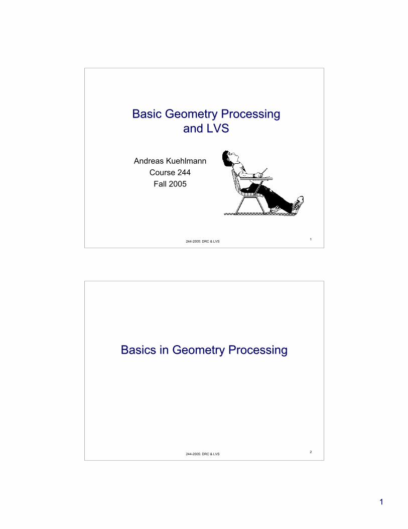
Forward Scanning PhaseForward Scanning Phase

• Maintain– L: Set of edges at current scanline position xcurr

• Count field for each edge records how many top and bottomedges on each side -> used for identifying regions

– S: Set of sets of edges that form a partition of L• Given unique label (integer between 1…m)

• Each set s ∈ S contains edges that are the boundary of aalready identified common output region

• Sets s1s2 ∈ S may be merged if during scanline move• S is maintained using UNION-FIND structure

• During processing produce temporary output file containing– Edge with label– Merging of two labels (merged label can be reused)– End of a label when region is processed

20244-2005: DRC & LVS

Processing of SProcessing of S

• When edge e becomes boundary (potential output edge)– Add e to corresponding set in S

– Create new s ∈ S for e if new region with new label

• When two boundary edges e1 and e2 intersect on scanline orcross scanline at the endpoint of a vertical boundary edge,– Write record for Merge e1 and e2

• When edge ceases to be boundary (results in output edge ewith e->xright=xcurr

– Write e(label) to temp file

• When set s ∈ S becomes empty– Write special record end(s)

1111

21244-2005: DRC & LVS

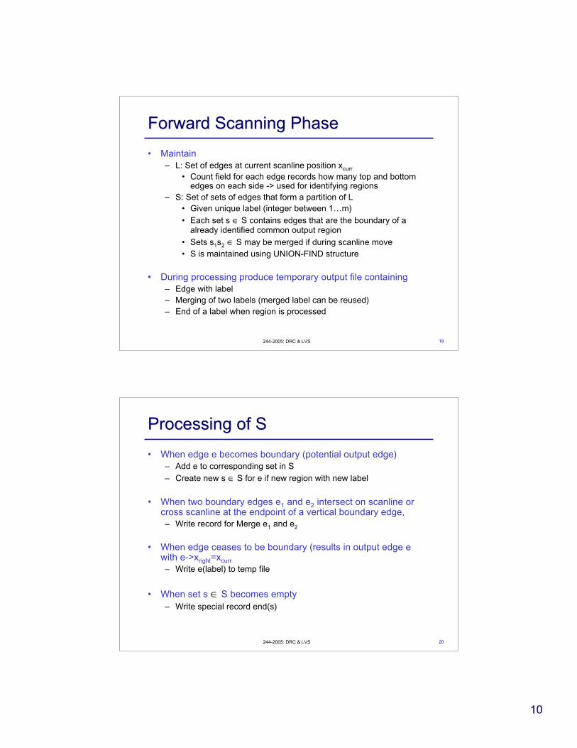
ExampleExample

0

0 {A,B}

2

2 {B,E},{C,D,F,G}

Xcurr S Output written

1

1 {B,E},{C,D} a(1)

a

4

4 {B,G,H,I} merge(2->1), e(1), d(1)

ed

5

5 {B,H,I,J} g(1)

g

7

7 ∅ b(1), j(1), end(1)

b

j

3

3 {B,E},{D,G,H,I} c(2), f(2)

fc

6

6 {B,J} i(1),h(1)

h

i

A

B

ED

CF

GI

H

J

K

22244-2005: DRC & LVS

Union-Find StructureUnion-Find Structure

• Three essential operations on elements x and y– Create-Set(x): Create a set containing a single element x

– Find-Set(x): Find the set that contains x

– Union(x,y): Merges the set containing x and another setcontaining y to a single set.After that operation:

– Find-Set(x) = Find-Set(y)

• Simple idea:– Put all elements in a tree data structure

– Root of tree is representative of set

– Root element points to itself

1

2

4

5

3

6

1212

23244-2005: DRC & LVS

Union-Find StructureUnion-Find Structure

Algorithm Create-Set(x) { create new vertex v

vertex->parent = vertex

}

x

1

2

43

Algorithm Find-Set(x) { while (x->parent != x) {

x = x->parent;

}

return x} x1

x2

x3

24244-2005: DRC & LVS

Implementation of MergeImplementation of Merge

Algorithm Merge(x,y) { x->parent = y->parent

}

1

2

3

4

5

• Problem:– May result in linear linked list, e.g.

– Merge(2,1)

– Merge(3,2)

– Merge(4,3)

– Merge(5,4)

– …

1313

25244-2005: DRC & LVS

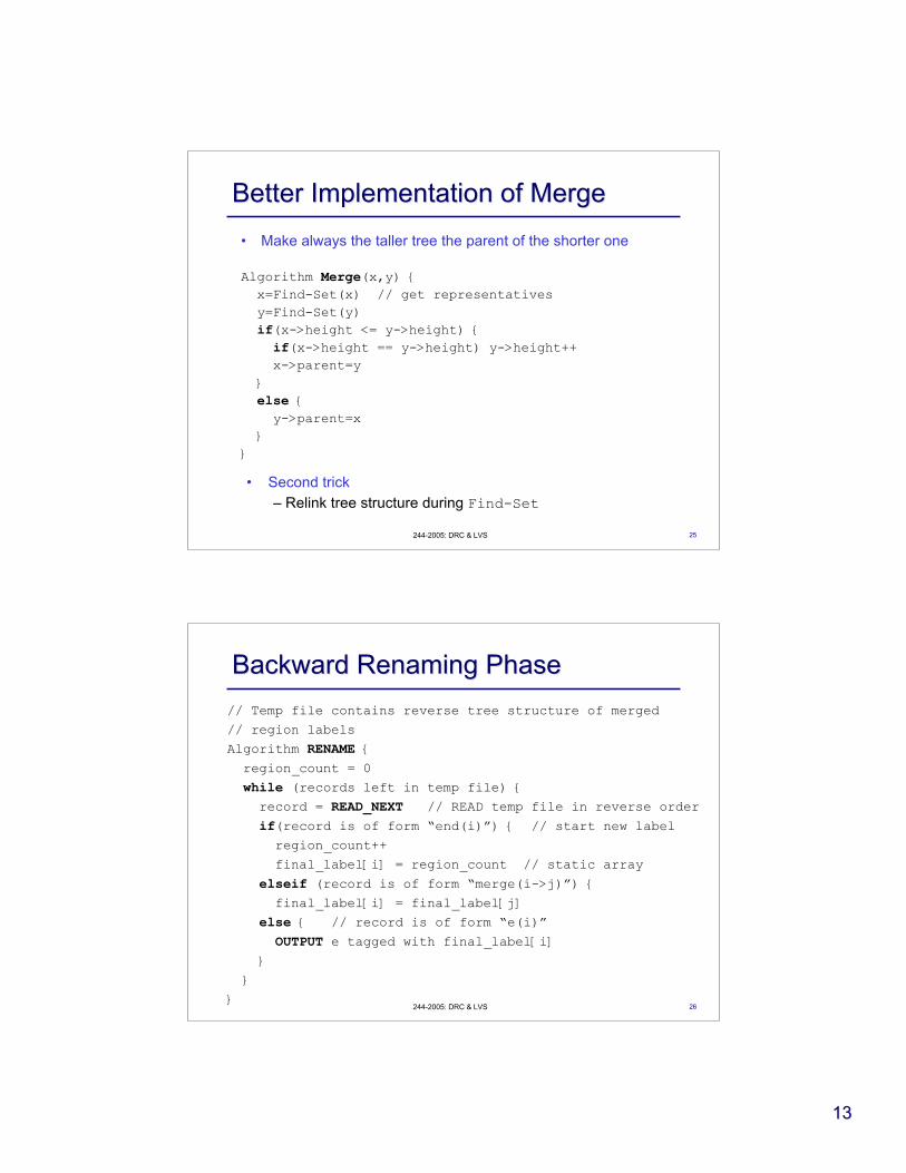
Better Implementation of MergeBetter Implementation of Merge

• Make always the taller tree the parent of the shorter one

Algorithm Merge(x,y) { x=Find-Set(x) // get representatives

y=Find-Set(y) if(x->height <= y->height) { if(x->height == y->height) y->height++ x->parent=y

} else { y->parent=x }

}

• Second trick– Relink tree structure during Find-Set

26244-2005: DRC & LVS

Backward Renaming PhaseBackward Renaming Phase

// Temp file contains reverse tree structure of merged

// region labels

Algorithm RENAME { region_count = 0

while (records left in temp file) { record = READ_NEXT // READ temp file in reverse order if(record is of form “end(i)”) { // start new label region_count++

final_label[i] = region_count // static array

elseif (record is of form “merge(i->j)”) { final_label[i] = final_label[j]

else { // record is of form “e(i)” OUTPUT e tagged with final_label[i] }

}

}

1414

27244-2005: DRC & LVS

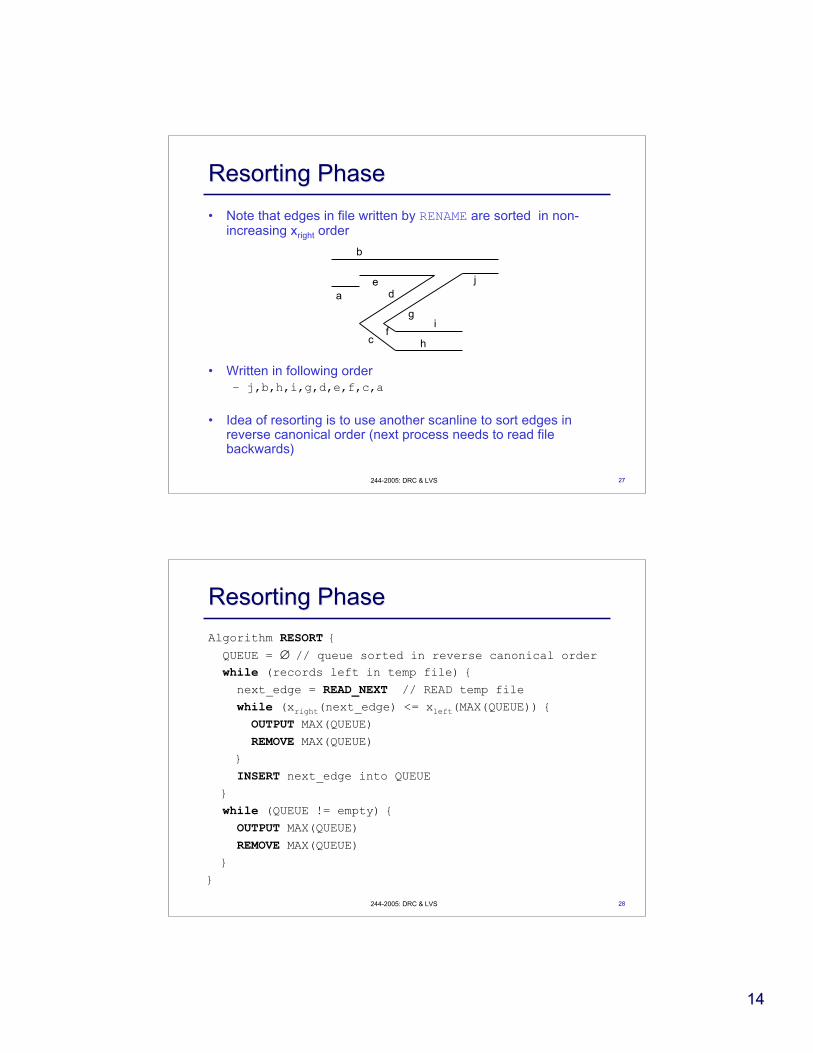
Resorting PhaseResorting Phase

• Note that edges in file written by RENAME are sorted in non-increasing xright order

• Written in following order– j,b,h,i,g,d,e,f,c,a

• Idea of resorting is to use another scanline to sort edges inreverse canonical order (next process needs to read filebackwards)

ae

d

g

b

j

fc h

i

28244-2005: DRC & LVS

Resorting PhaseResorting Phase

Algorithm RESORT { QUEUE = ∅ // queue sorted in reverse canonical order while (records left in temp file) { next_edge = READ_NEXT // READ temp file while (xright(next_edge) <= xleft(MAX(QUEUE)) { OUTPUT MAX(QUEUE) REMOVE MAX(QUEUE) }

INSERT next_edge into QUEUE }

while (QUEUE != empty) { OUTPUT MAX(QUEUE) REMOVE MAX(QUEUE) }

}

1515

29244-2005: DRC & LVS

Notes on Connectivity AnalysisNotes on Connectivity Analysis

• Algorithm is very general– Can handle multi-layer connectivities

• Process one scanline per layer in synchronous manner

• Maintain one set S for all layers

• Whenever via occurs between two layers

– Merge sets in S

• Use one temporary file and tag edge with layer number toseparate them during resorting phase

• Renaming and resorting phase can be pipelined

30244-2005: DRC & LVS

Diffusion

Polysilicon

Transistor IdentificationTransistor Identification

• MOS transistors are formed by intersection of diffusion andpolysilicon layer

Drain connection

Source connection

Gate connection

Active gate region

• Generate three edge files for transistor identification:– Active gate area (Poly & Diff) (trans_file)

– Polysilicon outside of active gate area (Poly & ^ Diff) (poly_file)

– Diffusion outside of active gate area (^Poly & Diff) (diff_file)

1616

31244-2005: DRC & LVS

Transistor IdentificationTransistor Identification

• Sweep scanline from left to right and process all transistoredges from trans file– For each edge processing:

• Maintain transistor record by transistor label

– Handles snaked and other weird transistors

• Read all diff edges and poly edge touching edge

• Build transistor record with using poly label, and diff label asconnection identifier for Gate, Drain and Source

– Check for illegal situations

• Transistor edge not adjacent to poly or diff edge

32244-2005: DRC & LVS

ImprovementsImprovements

• For large chips updating region counters become bottleneck– Requires a complete scanline sweep from bottom to top for each

xcurr

• Done after all edges starting at xcurr read in

• However regions change only locally– Processing of entire scanline is overkill

– Only required because of sea areas

• Solution: Convert layout into trapezoids– Reading of edges can be done in pairs

– Change area is now predictable

• Changes start as bottom of trapezoid

• Ends at top of trapezoid

1717

33244-2005: DRC & LVS

Design Rule CheckingDesign Rule Checking

• Most rules can be reduced to checking the maximum toleranceof an edge e1 from all other edges e2 with difference label– Checking can be reduced to checking both endpoints p or e1

• Search space can be reduced by excluding all edges e2 whichare father away than maximum design rule– W.l.o.g., assume we check for tolerance 1

– Split the horizontal chip into “swaths” of width 1

– Check for each endpoint p of edge e1 whether edge of somedifferent net lies within tolerance of 1

e1

p e2

34244-2005: DRC & LVS

Swath StructureSwath Structure

• Key of checking algorithm is that we need to check p onlyagainst edges with endpoints in swath i-1, i, or i+1

• Extend “lifetime” of edges during scanline algorithm to stayduring swath i+1, i, and i-1– Check endpoints in swath i

p

swath i-1

swath i

swath i+1

1818

35244-2005: DRC & LVS

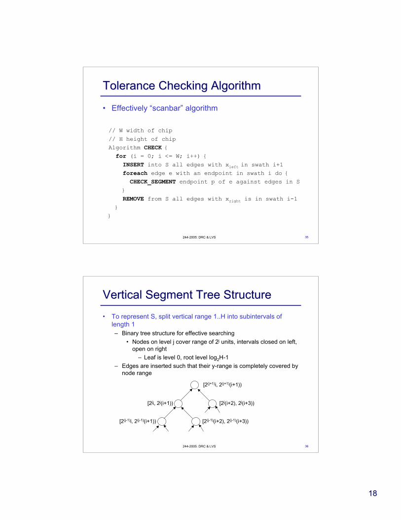
• Effectively “scanbar” algorithm

Tolerance Checking AlgorithmTolerance Checking Algorithm

// W width of chip

// H height of chip

Algorithm CHECK { for (i = 0; i <= W; i++) { INSERT into S all edges with xleft in swath i+1 foreach edge e with an endpoint in swath i do { CHECK_SEGMENT endpoint p of e against edges in S }

REMOVE from S all edges with xright is in swath i-1 }

}

36244-2005: DRC & LVS

Vertical Segment Tree StructureVertical Segment Tree Structure

• To represent S, split vertical range 1..H into subintervals oflength 1– Binary tree structure for effective searching

• Nodes on level j cover range of 2j units, intervals closed on left,open on right

– Leaf is level 0, root level log2H-1

– Edges are inserted such that their y-range is completely covered bynode range

[2(j+1)i, 2(j+1)(i+1))

[2ji, 2j(i+1)) [2j(i+2), 2j(i+3))

[2(j-1)i, 2(j-1)(i+1)) [2(j-1)(i+2), 2(j-1)(i+3))

1919

37244-2005: DRC & LVS

Vertical Segment Tree StructureVertical Segment Tree Structure

[0,4)

[0,2) [2,4)

[4,8)

[4,6) [6,8)

[0,8)

[0,1) [1,2) [2,3) [3,4) [4,5) [5,6) [6,7) [7,8)

e1(1,2) e3(3,4) e5(5,6) e7(7,8)

e6(6,7)e4(4,5)e2(2,3)

38244-2005: DRC & LVS

• Check interval that contains y(p) and its left and rightneighbor

Checking of Segment StructureChecking of Segment Structure

Algorithm CHECK_SEGMENT (p) { l = leaf in S that contains y(p)

while (l is not root(S)) { TEST p against all edges in l TEST p against all edges in l’s left neighbor TEST p against all edges in l’s right neighbor l = parent(l)

}

}

2020

39244-2005: DRC & LVS

ImprovementsImprovements

• Each endpoint is contained in two edges of polygons– If test is independent of slope, one can eliminate half of the tests,

e.d. test only

• bottom endpoint of left edge

• left endpoint of top edge

• top endpoint of right edge

• right endpoint of bottom edge

• On non-leaf segments, skip test of neighbors if y(p) is fatherthan interval border

• Edges in higher parts of S are checked more often– Use asymmetric segment tree with redundant entries for edges

40244-2005: DRC & LVS

Basic LVSBasic LVS

2121

41244-2005: DRC & LVS

LiteratureLiterature

• C. Ebeling and O. Zajicek: Validating VLSI Circuit Layout byWirelist Comparison, International Conference on ComputerAided Design (ICCAD-83) pp. 172-173, September 1983.

• C. Ebeling: Gemini II: A Second Generation Layout ValidationTool, IEEE International Conference on Computer Aided Design(ICCAD-88), pp. 322-325, November 1988

• M. Ohlrich, C. Ebeling, Eka Ginting and Lisa Sather: SubGemini:Identifying Subcircuits Using a Fast Subgraph IsomorphismAlgorithm, Design Automation Conference, June 1993. pp. 31-37

42244-2005: DRC & LVS

ProblemProblem

1. Compare two netlists on CMOS transistor level

System LevelSystem Level

Register Transfer LevelRegister Transfer Level

Gate LevelGate Level

Transistor LevelTransistor Level

Layout LevelLayout Level

Mask LevelMask Level

ComparisonComparison

Extracted Transistor Extracted Transistor NetlistNetlist

ExtractionExtraction

Layout LevelLayout Level

Transistor LevelTransistor Level

• Applications:• Layout verification

• Switch-level circuit simulation

• Functional equivalence checking

2222

43244-2005: DRC & LVS

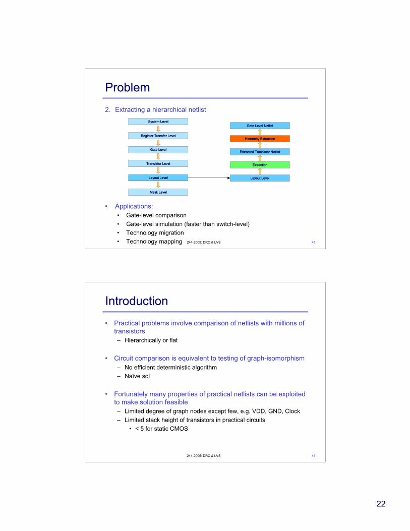
ProblemProblem

2. Extracting a hierarchical netlist

System LevelSystem Level

Register Transfer LevelRegister Transfer Level

Gate LevelGate Level

Transistor LevelTransistor Level

Layout LevelLayout Level

Mask LevelMask Level

Hierarchy ExtractionHierarchy Extraction

Gate Level Gate Level NetlistNetlist

ExtractionExtraction

Extracted Transistor Extracted Transistor NetlistNetlist

Layout LevelLayout Level

• Applications:• Gate-level comparison

• Gate-level simulation (faster than switch-level)

• Technology migration

• Technology mapping

44244-2005: DRC & LVS

IntroductionIntroduction

• Practical problems involve comparison of netlists with millions oftransistors– Hierarchically or flat

• Circuit comparison is equivalent to testing of graph-isomorphism– No efficient deterministic algorithm

– Naïve sol

• Fortunately many properties of practical netlists can be exploitedto make solution feasible– Limited degree of graph nodes except few, e.g. VDD, GND, Clock

– Limited stack height of transistors in practical circuits

• < 5 for static CMOS

2323

45244-2005: DRC & LVS

Graph PartitioningGraph Partitioning

• Use vertex invariants to classify vertices into equivalenceclasses– Based on attributes and degree of vertex

– Apply Hopcroft’s equivalence refinement until fixpoint reached

– Corresponding vertices in both graphs end up in one EC

Algorithm Partition { l(v) = initial label for vertex v

E’ = {(vi,vj) | l(vi)=l(vj)} do {

E = E’

E’= {(vi,vj) | l(vi)=l(vj) ∧ there is a pairwise mapping of all

adjacent vertices ui, uj suchthat

(ui,uj) ∈ E} } } while (E != E’)}

46244-2005: DRC & LVS

E3= {{v1},{v5},{v2},{v7},{v3},

{v6},{v4}}

{v4}E1= { , , }{v3,v6}{v1,v2,v5,v7}

v7v6v5

ExampleExample

v1 v2 v3

v4

v1 v2 v3

v7v6v5

v4

E2= {{v1,v5},{v2},{v7},{v3},

{v6},{v4}}

v1 v2 v3

v7v6v5

v4

2424

47244-2005: DRC & LVS

Using Neighbor SignaturesUsing Neighbor Signatures

v7v6v5

v1 v2 v3

v4

Sig(v1) = AAB

Sig(v2) = ABC

Sig(v3) = AABC

Sig(v4) = AB

Sig(v5) = AAB

Sig(v6) = AAAB

Sig(v7) = ABB

A

B

C

1. iteration:1. iteration:

v7v6v5

v1 v2 v3

v4

Sig(v1) = 3

Sig(v2) = 3

Sig(v3) = 4

Sig(v4) = 2

Sig(v5) = 3

Sig(v6) = 4

Sig(v7) = 3

Initialization:Initialization:

48244-2005: DRC & LVS

Using Neighborhood SignaturesUsing Neighborhood Signatures

v1 v2 v3

v7v6v5

Sig(v1) = ABD

Sig(v2) = ACF

Sig(v3) = BDEF

Sig(v4) = BC

Sig(v5) = ADE

Sig(v6) = AACE

Sig(v7) = ADC

A

B C

D E

Fv4

2. iteration:2. iteration:

v1 v2 v3

v7v6v5

Sig(v1) = G

Sig(v2) = B

Sig(v3) = C

Sig(v4) = F

Sig(v5) = A

Sig(v6) = D

Sig(v7) = E

A

B C

D E

Fv4

FixpointFixpoint::G

2525

49244-2005: DRC & LVS

ImplementationImplementation

• Hash signatures into computer word and store in linear array– May result in hash collisions, however, can be handled in post-

processing

• Sort array according to signature

• Single sweep over array to identify new boundaries ofequivalence classes– Refines old boundaries

• Refinements:– Second sorting criteria: size of the adjacent equivalence classes

– Refinement only on first top classes

• Idea: small equivalence classes lead to quick refinement oftheir neighbors

50244-2005: DRC & LVS

Implementation (2)Implementation (2)

Hash value for neighbors

Size of largestneighbor class

0x575467 4

0x575467 19

0x605566 2

0x605566 4

0x605566 34

0x946284 567

0x787734 7

0x787734 67

0x794383 424

0x805566 7

….

1. Sort array by signatures1. Sort array by signatures - neighbor class size as - neighbor class size as second criteria second criteria

2. Linear sweep to2. Linear sweep to mark class boundaries mark class boundaries

2626

51244-2005: DRC & LVS

Implementation (3)Implementation (3)

Hash value for neighbors

Size of largestneighbor class

0x605566 2

0x605566 4

0x605566 34

0x575476 4

0x575476 19

0x787734 7

0x787734 67

0x805566 7

0x794383 424

0x946284 567

….

3. Sort classes by smallest3. Sort classes by smallest neighbor class neighbor class

4. Update signatures for4. Update signatures for first n classes first n classes - e.g. classes of neighbor- e.g. classes of neighbor size 1 size 1

5. 5. Goto Goto 11

52244-2005: DRC & LVS

LVS AlgorithmLVS Algorithm

• Both circuits to be compared as bipartite graph– First set of vertices models transistors/gates

– Second set of vertices models nets

– Initial vertex invariants used for initial labeling

• Type of device for transistor/gate, number of terminals for net

• Terminal types (gate or drain/source)

• Length of smallest cycle containing vertex

P P

N

N

i2

i1

i1 i2

GND

VDD

g

gg

g d

d

d

dd d

d d

2727

53244-2005: DRC & LVS

LVS AlgorithmLVS Algorithm

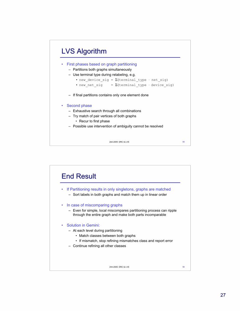
• First phases based on graph partitioning– Partitions both graphs simultaneously

– Use terminal type during relabeling, e.g.

• new_device_sig = Σ (terminal_type ⋅ net_sig)• new_net_sig = Σ (terminal_type ⋅ device_sig)

– If final partitions contains only one element done

• Second phase– Exhaustive search through all combinations

– Try match of pair vertices of both graphs

• Recur to first phase

– Possible use intervention of ambiguity cannot be resolved

54244-2005: DRC & LVS

End ResultEnd Result

• If Partitioning results in only singletons, graphs are matched– Sort labels in both graphs and match them up in linear order

• In case of miscomparing graphs– Even for simple, local miscompares partitioning process can ripple

through the entire graph and make both parts incomparable

• Solution in Gemini:– At each level during partitioning

• Match classes between both graphs

• If mismatch, stop refining mismatches class and report error

– Continue refining all other classes

2828

55244-2005: DRC & LVS

ImprovementsImprovements

• Dealing with series transistors– Serial transistors are exchangeable since no change of function

– Often done during late timing correction to accommodate for latearriving signals

– Solution: Keep them as one vertex and resolve later

- Can be done hierarchically

i2

P P

2

i2

i1

i1

GND

VDD

g

gg

g

d

dd d

d d

56244-2005: DRC & LVS

Improvements (2)Improvements (2)

• Symmetric circuit structures cause many iterations duringrefinements– E.g. ring oscillators, rotator circuits, highly regular data-paths

• Local matching– Checks pairs of already matched vertices and matches them based

on local information

• Partitioning done only on neighbor vertices

• Continues until no new matches found

• Interleaved with global repartitioning

• Miscompares can be refined by local matches– One circuit declared as golden

– Local matches applied on mismatched equivalence class

2929

57244-2005: DRC & LVS

SubcircuitSubcircuit Identification Identification

• Used in building hierarchy– Problem is now subgraph isomorphism

• Basic algorithm– Phase 1:

• Use graph partitioning to find candidate vector for eachsubcircuit S in circuit G

– Ensure that terminal net invariants are not used asconnectivity not known yet (corrupt vertices)

– Candidate vector stored as set of key vertices which arepotential matches

– Phase 2:• Continue relabeling phase of partitioning algorithm to confirm

matches in circuit– Done in parallel for all subcircuits (e.g. library)

58244-2005: DRC & LVS

ExampleExample

Subcircuit: Circuit:

P P

N

N

P P

N

N

N

N

P

S: G:

noncorrupt

corrupt

3030

59244-2005: DRC & LVS

Phase 1Phase 1

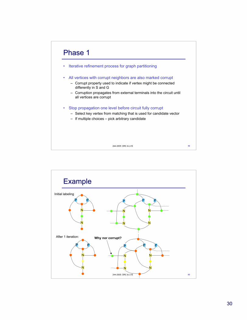
• Iterative refinement process for graph partitioning

• All vertices with corrupt neighbors are also marked corrupt– Corrupt property used to indicate if vertex might be connected

differently in S and G

– Corruption propagates from external terminals into the circuit untilall vertices are corrupt

• Stop propagation one level before circuit fully corrupt– Select key vertex from matching that is used for candidate vector

– If multiple choices – pick arbitrary candidate

60244-2005: DRC & LVS

ExampleExample

P P

N

N

P P

N

N

N

N

P

Initial labeling

Why nor corrupt?

P P

N

N

P P

N

N

N

N

P

After 1 iteration:

3131

61244-2005: DRC & LVS

Phase 2Phase 2

• Process candidate vector in G to confirm matches

• Modified partitioning algorithm– Starts from key vertices and matches them

– Propagate through both graphs S and G and update labelsaccording to modified relabeling function

– Ensure that other partitions do not spoil label function