Baseline Energy Consumption and Greenhouse Gas Emissions In Commercial Buildings in Australia Part 1 - Report November 2012

Council of Australian Governments (COAG) National Strategy on Energy Efficiency

Baseline Energy Consumption and Greenhouse Gas Emissions in Commercial Buildings in Australia – Part 1 - Report

Prepared by pitt&sherry with input from BIS Shrapnel and Exergy Pty Ltd

Published by the Department of Climate Change and Energy Efficiency

www.climatechange.gov.au

ISBN: 978-1-922003-81-2 © Commonwealth of Australia 2012 This work is licensed under the Creative Commons Attribution 3.0 Australia Licence. To view a copy of this license, visit http://creativecommons.org/licenses/by/3.0/au The Department of Climate Change and Energy Efficiency asserts the right to be recognised as author of the original material in the following manner:

or © Commonwealth of Australia (Department of Climate Change and Energy Efficiency) 2012. IMPORTANT NOTICE – PLEASE READ This document is produced for general information only and does not represent a statement of the policy of the Commonwealth of Australia. The Commonwealth of Australia and all persons acting for the Commonwealth preparing this report accept no liability for the accuracy of or inferences from the material contained in this publication, or for any action as a result of any person’s or group’s interpretations, deductions, conclusions or actions in relying on this material. Acknowledgment As part of the National Strategy on Energy Efficiency the preparation of this document was overseen by the Commercial Buildings Committee, comprising officials of the Department of Climate Change and Energy Efficiency, Department of Resources, Energy and Tourism and all State and Territory governments.

i

Table of Contents Index of Tables ................................................................................................. iii Index of Figures ................................................................................................. iv Glossary ........................................................................................................... v Abbreviations ................................................................................................... xi 1. Executive Summary ...................................................................................... 1

Overall Conclusions ...................................................................................... 9 2. Introduction ............................................................................................. 11

2.1 Background ..................................................................................... 11 2.2 Project Objectives and Scope ............................................................... 11 2.3 Policy Context .................................................................................. 13 2.4 The Project Team ............................................................................. 13

3. Overview of Methodology ............................................................................. 15 3.1 Stock Model ..................................................................................... 15 3.2 Energy Consumption Data .................................................................... 17 3.3 Data Analysis and Model Construction ..................................................... 19 3.4 Model Validation ............................................................................... 20 3.5 Statistical Confidence ........................................................................ 20 3.6 Key Assumptions ............................................................................... 21

4. Key Issues ................................................................................................ 24 4.1 The Building Stock ............................................................................. 24 4.2 Energy Performance Data .................................................................... 26 4.3 Model Scope and Resolution ................................................................. 29 4.4 Overarching Conclusions ..................................................................... 31

5. Offices .................................................................................................... 32 5.1 Introduction .................................................................................... 32 5.2 Stock Estimates - Offices ..................................................................... 32 5.3 Energy Intensity - Standalone Offices ...................................................... 35 5.4 Total Energy Consumption and Greenhouse Gas Emissions - Standalone Offices .. 40 5.5 Energy End Use - Offices ..................................................................... 42 5.6 State and Territory Estimates - Standalone Offices ..................................... 46 5.7 Government Owned Standalone Offices ................................................... 49 5.8 Conclusions - Offices .......................................................................... 51

6. Hotels .................................................................................................... 53 6.1 Introduction .................................................................................... 53 6.2 Stock Estimates - Hotels ...................................................................... 53 6.3 Energy Intensity - Hotels ..................................................................... 53 6.4 Total Energy Use and Greenhouse Gas Emissions - Hotels ............................. 55 6.5 Energy End Use - Hotels ...................................................................... 56 6.6 State and Territory Results - Hotels ........................................................ 57 6.7 Conclusions - Hotels ........................................................................... 59

7. Retail Buildings ......................................................................................... 60 7.1 Introduction .................................................................................... 60 7.2 Stock Estimates - Retail ...................................................................... 60 7.3 Energy Intensity - Retail ...................................................................... 64 7.4 Total Energy Consumption and Greenhouse Gas Emissions - Retail .................. 67 7.5 Energy End Use - Retail ....................................................................... 69 7.6 States and Territory Estimates - Retail .................................................... 69 7.7 Conclusions - Retail ........................................................................... 71

8. Hospitals ................................................................................................. 72 8.1 Introduction .................................................................................... 72 8.2 Stock Estimates - Hospitals .................................................................. 72 8.3 Energy Intensity - Hospitals .................................................................. 74 8.4 Total Hospital Energy Use and Greenhouse Gas Emissions ............................. 74 8.5 Energy End Use - Hospitals ................................................................... 75 8.6 State and Territory Estimates - Hospitals ................................................. 76 8.7 Conclusions - Hospitals ....................................................................... 78

9. Schools ................................................................................................... 79 9.1 Introduction .................................................................................... 79

ii

9.2 Stock Estimates - Schools .................................................................... 79 9.3 Energy Intensity - Schools .................................................................... 81 9.4 Total Energy Consumption and Greenhouse Gas Emissions - Schools ................ 81 9.5 Energy End Use - Schools ..................................................................... 82 9.6 State and Territory Estimates - Schools ................................................... 83 9.7 Conclusions - Schools ......................................................................... 85

10. Tertiary Education Buildings ......................................................................... 86 10.1 Introduction .................................................................................... 86 10.2 Stock Estimates - Tertiary Education ...................................................... 86 10.3 Energy Intensity - Tertiary Education Buildings .......................................... 89 10.4 Total Energy Consumption and Greenhouse Gas Emissions - Tertiary Education .. 91 10.5 Energy End Use - Universities ............................................................... 93 10.6 States and Territory Estimates - Tertiary Education .................................... 94 10.7 Conclusions - Tertiary Education ........................................................... 95

11. Public Buildings ......................................................................................... 96 11.1 Introduction .................................................................................... 96 11.2 Stock Estimates - Public Buildings .......................................................... 96 11.3 Energy Intensity - Public Buildings ........................................................ 100 11.4 Total Energy and Greenhouse Gas Emissions - Public Buildings ...................... 102 11.5 Energy End Use - Public Buildings ......................................................... 103 11.6 State and Territory Estimates - Public Buildings ........................................ 105 11.7 Conclusions - Public Buildings .............................................................. 108

Appendix A Statement of Requirements

Appendix B Bibliography

Appendix C Model Documentation

Appendix D Top-down Model Validation

Appendix E Statistical Analysis

iii

Index of Tables Table 1.1- Non-Residential, Non-Industrial Building Stock, Australia, 1999-2020 (floor area in ‘000m2) ........................................................................................................... 2 Table 1.2 - Total Energy Use and Greenhouse Gas Emissions: Australia, 1999-2000, Non-Residential Buildings ............................................................................................ 3 Table 1.3 - Australian Average Energy Intensity Trends by Building Type, 1999 – 2020 ...... 8 Table 3.1 - Energy Data Records and Individual Building Counts by Building Type ........... 18 Table 3.2 – Recommended Minimum Sample Sizes per Year .......................................... 21 Table 3.3 - Population Growth, 1999 to 2020 (millions) ............................................... 23 Table 5.1 - Stand-Alone Office Stock by State and Region, 1999 to 2020 (‘000 m2 NLA) ........ 33 Table 5.2 - Non-Stand-Alone Office Stock by State and Region, 1999 to 2020 (‘000m2 NLA) ... 34 Table 5.3 - Energy Use and Greenhouse Gas Emissions, Standalone Offices by Sub-Type, 1999-2020 ............................................................................................................. 41 Table 5.4 - Standalone Offices, Whole Buildings, Energy Consumption by Fuel, 1999 to 2020, Australia ........................................................................................................ 42 Table 5.5 - Standalone Office Tenancy Energy Consumption by State and Territory ............ 46 Table 5.6 - Standalone Office Base Building Energy Consumption by State and Territory ...... 46 Table 5.7 - Standalone Office Whole Buildings Energy Consumption by State and Territory ... 47 Table 5.8 - Privately Owned Standalone Office Tenancies, Average Energy Intensity by State, Territory and Region (n > 50/year), 1999 – 2012 ........................................................ 48 Table 5.9 - Privately Owned Standalone Office Base Buildings, Average Energy Intensity by State, Territory and Region (n > 50/year), 1999 – 2012 ............................................... 48 Table 5.10 - Privately Owned Standalone Office Whole Buildings, Average Energy Intensity by State, Territory and Region (n > 30/year), 1999 – 2012 ............................................... 48 Table 5.11 - Government Owned Standalone Office Tenancies, Average Energy Intensity by State, Territory and Region (n > 50/year), 1999 – 2012 ............................................... 49 Table 5.12 - Government Owned Standalone Office Whole Buildings, Average Energy Intensity by State, Territory and Region (n > 30/year), 1999 – 2012 ............................................ 50 Table 5.13 - Sample Size Summary, Government-Owned Offices by State and Region, All Periods .......................................................................................................... 51 Table 5.14 - Sample Size Summary, Privately-Owned Offices by State and Region, All Periods 52 Table 6.1 - Hotel Stock by State and Region, 1999 to 2020 (‘000 m2 NLA) ......................... 54 Table 6.2 - Hotels, Energy Consumption by Fuel, and GHG Emissions 1999 to 2020, Australia . 56 Table 6.3 - Hotel Energy Consumption by State and Territory .................................... 58 Table 6.4 - Hotels, Average Energy Intensity by State, Territory and Region (n > 5/year), 1999 – 2012 ............................................................................................................. 58 Table 7.1- Shopping Centre Stock Estimates by State and Region, 1999 – 2020 (‘000 m2 GFA) 61 Table 7.2- Supermarket Stock Estimates by State and Region, 1999 – 2020 (‘000 m2 GFA) ..... 62 Table 7.3 - Retail Strip Stock Estimates by State and Region, 1999 – 2020 (‘000 m2 GFA) ...... 63 Table 7.4 - Retail: Energy Use and Greenhouse Gas Emissions, 1999 – 2020 ....................... 67 Table 7.5 - Shopping Centre Total Energy Consumption by State, 2009 and 2020, PJ ........... 69 Table 7.6 - Shopping Centre Retail Tenancies Energy Consumption by State, 2009 and 2020, PJ ................................................................................................................... 70 Table 7.7 - Shopping Centre Base Building Energy Consumption by State, 2009 and 2020, PJ . 70 Table 7.8 - Supermarket Total Energy Consumption by State, 2009 and 2020, PJ ................ 70 Table 7.9 - Stand-alone Supermarket Energy Consumption by State, 2009 and 2020, PJ ....... 71 Table 8.1 – All Hospital Stock by State and Region, 1999 to 2020 (‘000 m2) ....................... 73 Table 8.2 - Total Energy Use and Greenhouse Gas Emissions, Hospitals, 1999-2020 ............. 75 Table 8.3 - Hospital Energy Consumption by State and Territory .................................... 77 Table 8.4 - Public Hospitals, Average Energy Intensity by State, Territory and Region (n >= 10/year), 1999 – 2012 ........................................................................................ 78 Table 9.1 - School Stock (public and private) by State and Region, 1999 to 2020 (‘000 m2 NLA) ................................................................................................................... 80 Table 9.2 - Total Energy Consumption and Greenhouse Gas Emissions, Schools, 1999-2020.... 82 Table 9.3 - Schools Energy Consumption by State and Territory ..................................... 84 Table 9.4 - Public Schools, Average Energy Intensity by State, Territory and Region (n >= 10/year), 1999 – 2012 ........................................................................................ 84 Table 10.1 - Stock Estimates, TAFE/VET Floor Area, 1999 – 2020, ‘000m2 ......................... 87 Table 10.2 - Stock Estimates, University Floor Area, 1999 – 2020, ‘000m2 ......................... 88 Table 10.3 - Total Energy Consumption and Greenhouse Gas Emissions, Vocational Education and Training (VET) Buildings, Australia, 1999 – 2020 ................................................... 91

iv

Table 10.4 - Total Energy Consumption by Fuel and Greenhouse Gas Emissions, Universities, Australia, 1999 – 2020 ........................................................................................ 92 Table 10.5 - Vocational Education and Training Buildings, Total Energy Consumption by State, 1999, 2009, 2020 .............................................................................................. 94 Table 10.6 - University Buildings, Total Energy Consumption by State, 1999, 2009, 2020 ...... 95 Table 11.1 - Public Building Stock by State and Region, 1999 to 2020 (‘000 m2 NLA) ............ 97 Table 11.2 - Law Court Stock by State and Region, 1999 to 2020 (‘000 m2 NLA) ................. 98 Table 11.3 - Correctional Centre Stock by State and Region, 1999 to 2020 (‘000 m2 NLA) ..... 99 Table 11.4 - Public Buildings, Energy Consumption by Fuel, and GHG Emissions, 1999 to 2020, Australia ....................................................................................................... 103 Table 11.5 - Total Energy Consumption, Fuel Use and Greenhouse Gas Emissions, Law Courts, Australia, 1999 – 2020 ....................................................................................... 104 Table 11.6 - Public Buildings, Average Energy Intensity by State, Territory and Region (where n>= 10/year), 1999 – 2012 .................................................................................. 106 Table 11.7- Public Buildings, Energy Consumption by State, 1999, 2009, 2020 (PJ) ............ 106 Table 11.8 - Law Courts, Average Energy Intensity by State (where n>=6/year), 1999 – 2011 107 Table 11.9- Law Courts, Energy Consumption by State, 1999, 2009, 2020 (PJ) .................. 107 Index of Figures Figure 1.1 - Total Energy Consumption by Building Type, 2009 (PJ, % shares) ...................... 5 Figure 1.2 - Total Energy Consumption by Building Type, 2020 (PJ, % shares) ...................... 5 Figure 1.3 - Total Energy Consumption: Non-Residential, Non-Industrial Buildings, Australia, 2009 to 2020 (PJ) ............................................................................................... 6 Figure 1.4 - Fuel Mix, All Buildings, 2009 (% shares) ..................................................... 6 Figure 1.5 - Offices (All), Electricity End Use Shares, 1999 - 2012 .................................... 7 Figure 1.6 - Projected Greenhouse Gas Emissions, All Non-Residential, Non-Industrial Buildings, 2009 to 2020 ..................................................................................................... 9 Figure 3.1 - NRBuild Model Schematic .................................................................... 16 Figure 3.2 - Greenhouse Gas Intensity of Electricity Supply by State, 2009 (kg CO2-e/kWh) ... 22 Figure 5.1 - Standalone Office Stock by State Historical and Projections, 1999 to 2020 ........ 35 Figure 5.2 - Non-Standalone Office Stock by State, Historical and Projections, 1999 to 2020 . 36 Figure 5.3 - Total Energy Intensity versus Area, All Offices........................................... 36 Figure 5.4 - Average Energy Intensity, Office Tenancies, Australia ................................. 37 Figure 5.5 - Average Energy Intensity, Office Base Buildings, Australia ............................ 38 Figure 5.6 - Whole Office Building Energy Intensity, Australia, cf Base Building + Tenancy Energy Intensity (MJ/m2.a) ................................................................................. 39 Figure 5.7 - Whole Office Building Energy Intensity, Australia, cf Base Building + Tenancy Energy Intensity without OSCAR data ..................................................................... 40 Figure 5.8 - Office Tenancies, Electricity End Use Shares, 1999 – 2012 ............................ 43 Figure 5.9 - Office Base Buildings, Electricity End Use Shares, 1999 – 2012 ....................... 44 Figure 5.10 - Office Base Buildings, Natural Gas End Use Shares, 1999 - 2012 .................... 44 Figure 5.11 - Offices (All), Electricity End Use Shares, 1999 - 2012 ................................. 45 Figure 5.12 - Offices (All), Natural Gas End Use Shares, 1999 - 2012 ............................... 45 Figure 6.1 - Hotel Energy Intensity, Australia (MJ/m2.a) .............................................. 55 Figure 6.2 - Hotels- Electrical End Use Shares, 1999 – 2012 .......................................... 57 Figure 6.3 - Hotels- Natural Gas End Use Shares, 1999 – 2012 ........................................ 57 Figure 8.1 - Hospitals Energy Intensity, Australia, (MJ/m2.a) ........................................ 74 Figure 8.2 - Hospitals- Electrical End Use Shares, 1999 – 2012 ....................................... 76 Figure 8.3 - Hospitals-Gas End Use Shares, 1999 – 2012 ............................................... 76 Figure 9.1 - Average Energy Intensity, Schools, Australia ............................................. 81 Figure 9.2 - ACT Schools, Electrical End Use Shares, 1999 – 2012 ................................... 83 Figure 9.3 - ACT Schools, Natural Gas End Use Shares, 1999 – 2012 ................................. 83 Figure 10.1 - Average Energy Intensity, VETs, Australia, 2003 – 2010 ............................... 90 Figure 10.2 - Average Energy Intensity, Universities, Australia, 2001 – 2011 ...................... 90 Figure 10.3 - VET Buildings– Fuel Shares, Australia 2010 .............................................. 92 Figure 10.4 - University Buildings Fuel Shares, Australia, 2009 ...................................... 93 Figure 10.5 - Universities- Electrical End Use Shares, Australia, 1999 – 2012 ..................... 93 Figure 11.1 - Public Building Average Energy Intensity, Australia, 2001 - 2010 (MJ/m2.a) .... 101 Figure 11.2 - Average Energy Intensity, Law Courts, Australia, 1999 - 2011 ...................... 102 Figure 11.3 - Law Courts- Electrical End Use Shares, Australia, 1999 - 2011 ..................... 105 Figure 11.4 - Law Courts- Natural Gas End Use Shares, Australia, 1999 – 2011 .................. 105

v

Glossary Abatement An activity that leads to a reduction in greenhouse gas emissions.

Activity In the context of energy efficiency, activity refers to the output associated with energy use when the output is not a physical product. An example is space heating or cooling in the residential and commercial sectors.

Base Building The common areas of a building which are served by central services.

Baseline A projected level of future emissions or energy use against which reductions by project activities could be determined; or the emissions or energy use that would occur without policy intervention.

Behaviour Energy user or equipment operator behaviours that affect energy consumption.

Bottom-up model A method of estimation whereby the individual components that make up a project are estimated separately. The individual results are then aggregated to produce an estimate of the entire project. In the context of this study, estimates of the energy use of individual buildings are aggregated to estimate the total energy use of all the relevant building stock.

Carbon dioxide equivalent (CO2-e)

Greenhouse gases include carbon dioxide, methane, and nitrous oxide, with each gas having different physical properties and global warming potential. It is conventional to express all gas emissions in “equivalent amounts of carbon dioxide” where “equivalent” means “having the same global warming potential over a period of 100 years”.

Co-generation Combined production of electricity and useful heat (for hot water or space heating) from the same process. Also known as combined heat and power.

Confidence level Using sample data to make conclusions and estimates about the population is not always going to be correct. For this reason, a measure of reliability has been built into the statistical inference. The confidence level is the proportion of times that an estimating procedure will be correct. In this project, the minimum sample size is that required in order to ensure that estimates based on this energy data will be correct 95% of the time.

Cost-effective A measure is cost effective when the present value of the benefits attributable to the measure exceeds the present value of the costs at a given discount rate. When these two values are expressed as a ratio (a benefit cost ratio or BCR), a cost effective measure will have a BCR of at least 1.

Database (or set) A collection of data records relating, in this context, to a particular building type.

Duty cycle The work or actions which an appliance or piece of equipment performs over a set period of time which is representative of the pattern of work or actions performed over the whole life of the appliance or equipment. The annual energy use of equipment is a function of numerous variables – one of the most important is the duty cycle.

Embedded generation Production of electricity from power stations which are connected to the distribution network (as opposed to the transmission network). Generally these range from small household solar PV systems to medium scale with capacity less than 30 MW. In Australia, distributed generation most often relates to diesel, gas (including cogeneration) or renewables (including solar, wind, micro hydro or biomass). Also referred to as “distributed generation”, or “on-site generation”.

Emissions The release of greenhouse gases to the atmosphere.

vi

Emissions intensity An amount of emissions (CO2-e) per a specified unit of output (e.g. GDP, sales revenue or goods produced).

End use technology/process data

Data regarding the nature of the stock of end-use and conversion technologies.

Energy conversion The process of converting energy from one form to another. Power stations for instance convert “primary” fuels or renewable energy into ‘secondary’ or ‘final’ forms, such as electricity. A boiler transforms coal, gas, electricity or other fuels into heat in the form of steam. Each conversion process involves losses of useful energy, with the greater the loss, the lower the energy efficiency.

Energy efficiency (general)

The amount of useful work that can be performed by an energy using system per unit of energy consumption. It is generally expressed as a ratio: useful output to energy input. A piece of equipment or system is described as more energy efficient to the extent that it performs more useful work for the same energy consumption, or else performs the same amount of useful work for less energy consumption. The concept is only applicable to narrowly defined energy using systems. For complex systems, such as a manufacturing plant, or a whole sector the number of energy using processes and variables affecting energy use are too great to measure energy efficiency in this strict sense.

Energy end use The point at which energy is used in the provision of a final product or service, rather than producing another form of energy.

Energy intensity The ratio of energy input to useful output.

Energy performance Measurable results relating to energy use and consumption. The term includes energy efficiency, energy intensity, energy conservation, fuel choice and greenhouse gas emissions resulting directly and indirectly from energy use.

Energy services Useful energy or work provided by an energy-using system. The services may include heating, cooling, mechanical work or electrical system outputs (computing, communications, etc).

Equipment level energy end use

The consumption of energy measures at the level of individual pieces of equipment at a site. The term is most commonly used to describe energy use, in residential and commercial buildings, manufacturing facilities or mine sites, disaggregated to the level of, for instance, a refrigerator, a chiller, a boiler, a kiln, or a grinding mill. Also referred to as “equipment energy end use”.

Environmental data A range of environmental or climate variables that may affect the efficiency of energy-using processes. Examples include “degree days” as a proxy for external heat loads on a structure, or “relative humidity” that may affect combustion efficiency.

Explanatory data A broad term covering information about factors that may influence energy efficiency and energy intensity, such as weather, duty cycle, prices, exchange rates and many other factors.

Field Data point of a certain type – such as ‘Financial Year’ or ‘Street Address’. Data records are comprised of such fields.

Finite population Where the population is not infinitely large. Generally, if the sample size is greater than 1% of the population, the population is assumed to be finite. In the calculations for the minimum number of buildings required, assuming an infinite population means that the minimum number of buildings required to achieve the prescribed confidence level and accuracy could exceed the actual number of buildings available in a particular region. In such a situation, the population is considered finite and the associated calculations assume finite population size.

vii

Fully Enclosed Covered Area (FECA)

The sum of all such areas at all building floor levels, including basements (except unexcavated portions), floored roof spaces and attics, garages, penthouses, enclosed porches and attached enclosed covered ways alongside buildings, equipment rooms, lift shafts, vertical ducts, staircases and any other fully enclosed spaces and usable areas of the building, computed by measuring from the normal inside face of exterior walls but ignoring any projections such as plinths, columns, piers, and the like which project from the normal inside face of exterior walls. It shall not include open courts, light wells, connecting or isolated covered ways and net open areas of upper portions of rooms, lobbies, halls, interstitial spaces and the like, which extend through the storey being computed (Altus Page Kirkland, 2012).

Final energy use The total amount of energy consumed in the final or end use energy sectors. It is equal to primary energy use less energy consumed or lost in conversion, transmission and distribution.

Fuel mix The mix of fuel types within a given amount of energy consumption.

Greenhouse gases The atmospheric gases responsible for causing global warming and climate change. The major greenhouse gases are carbon dioxide (CO2), methane (CH4), nitrous oxide (N20), hydrofluorocarbons (HFCs), perfluorocarbons (PFCs) and sulphur hexafluoride (SF6).

GreenPower Certified renewable energy that is delivered to an end user by an energy supplier.

Gross Floor Area (GFA) The sum of ‘fully enclosed covered area’ and ‘unenclosed covered area’ as defined.

Gross Lettable Floor Area Retail (GLAR)

The floor space contained within a retail tenancy measured from the internal finished surface of external building walls or passageways, but excluding features such as balconies and verandahs.

Infinite population Where the population is assumed to be infinitely large. Generally, if the sample size is less than 1% of the population, the population is assumed to be infinite.

Mean In computing numerical descriptive measures of the data, interest usually focuses on two measures: (1) a measure of the central, or average, value of the data and (2) a measure of the degree to which the observations are spread out about this average value. The mean measures the central location of the data, also expressed as the ‘average’ in this project.

Metrics Measurement units associated with a quantitative measure, such as ‘thousands of square metres of floor area’, or Petajoules (PJ) of energy.

Minimum energy performance standards (MEPS)

Regulatory requirements for appliances or equipment manufactured or imported to Australia to ensure a set level of energy efficiency performance is met or exceeded. MEPS typically cover appliances such as refrigerators, air conditioners and televisions.

Net Lettable Area (NLA) The sum of all lettable areas within a commercial type building, measured from the internal finished surfaces of permanent walls and from the internal finished surfaces of dominant portions of the permanent outer building walls, and including the area occupied by structural columns and engaged perimeter columns, as defined by the Property Council of Australia.

viii

Network losses Energy losses incurred in transporting energy over a network. It can include: heat lost through resistance in electricity wires, gas leaks, metering errors and theft. It can also include energy used in operating the network — such as gas consumed to run compressors in gas pipelines.

Online System for Comprehensive Activity Reporting (OSCAR)

A web-based data tool to record energy and emissions data for government program reporting. OSCAR standardises reporting from corporations and government. OSCAR calculates greenhouse gas emissions based on energy and emissions data.

Peak demand The maximum demand recorded in a given area. In the electricity market, to ensure reliability, supply capacity (generation and network) must be greater than the peak demand. Peak demand may only occur a few hours a year and is often driven by temperature due to heating and cooling loads. The term “peak load” is used interchangeably.

Population A population is the set of all items of interest in a statistical problem. For example, the population referred to in this project will be the actual number of buildings within a prescribed category, e.g. actual number of government owned office buildings in NSW.

Precinct A collection of buildings at the same location, often but not necessarily with the same owner. Schools, hospitals, universities, airports are all examples of precincts. Importantly for this study, building types (by function) may well vary within a precinct, and this variation is often not captured in statistical data.

Primary energy The total energy consumed of each primary fuel (in energy units) in both the transformation and end use sectors. It includes the use of primary fuels in transformation activities—notably the consumption of fuels used to produce petroleum products and electricity. It also includes own use and losses in the energy transformation sector. It excludes the consumption of secondary energy sources such as electricity and petroleum products.

Process energy use The level at which energy is used by individual systems or processes at a site. The term is most commonly used to describe energy use, in commercial buildings, manufacturing facilities or mine sites, disaggregated to the level of, for instance, cooling, steam production and grinding. Also referred to as “system level”.

Quality factors Changes in the nature, composition, performance specifications of inputs, processes or outputs. In this context, changes in qualitative factors or specifications can significantly affect measured energy consumption, particularly over longer periods of time. For example, it not strictly correct to compare the energy consumption of a house or a car from 1940 with one from 2012, as the nature of the house and car (in terms of the “services” they provide) has itself changed through time.

R2 A statistical measure that indicates the proportion of the variance in one data series that is attributable to the variance in another. Generally it is applied in this report to indicate the extent to which a best fit trendline (e.g., for average energy intensity) explains the variance in calculated data points.

Record A collection of data points or fields relating, in this context, to a single building in a single year.

ix

Regression Regression is used to predict the value of one variable on the basis of other variables. The coefficient of determination, denoted R2, measures the strength of the linear relationship between two variables. In this project, R2 is often predominantly used to describe the linear relationship between financial years and average EUI. The higher the value of R2, the better the model fits the data.

Renewables Energy sources that are constantly renewed by natural processes over a short recharge cycle. These include “flow” resources, such as solar, wind, wave and tidal energy, and some “storage” resources, including hydropower and some forms of biomass. Recharge cycles are generally limited to one year, to allow for seasonal restoration of dam storages and biomass resources, also this definition is contested.

Sample A sample is a set of data drawn from the population. In this project, the sample data is the energy data collating for each category. A descriptive measure of a sample is called a statistic. We use statistics to make inferences about the population (e.g., use the proportion of commercial buildings energy data collected to make inferences about general characteristics of all commercial buildings in Australia).

Standard deviation The standard deviation is a measure of variability that is expressed in the same units as the original data/observations, as is the mean. It is merely the square root of variance, which measures the variability of a set of quantitative data.

Standard Error The standard error referred to in this report is the standard deviation of the mean. It is also referred to as ‘accuracy’ in this report.

Stationary energy Energy produced and used by stationary equipment. Includes energy used for electricity generation; and fuels consumed in other sectors such as gas in the manufacturing and mining sectors and wood in the residential sector.

Stock A measure of the physical extent of buildings in Australia, such as the number or area of buildings.

Structural data Data that reveal, at the level of sectoral disaggregation being examined, changes in the composition of activity or the mix of production. For example data on end use equipment stocks layered by size, efficiency, age or other parameters. Structural factors vary by sector.

Top-down estimation In the context of this study, it is a method for estimating the overall or aggregate energy use of all the relevant building stock. Unlike a bottom-up estimation, it does not rely on estimating the individual components of a project and then adding them up.

T-test A t-test tests and estimates the difference between two population means by assuming the distribution is normal. T-tests are conducted wherever we have claimed or drawn conclusions about two means (e.g. the average EUI of capital cities buildings is higher than regional buildings) to test the difference between the two means. If the p-value of the test is small, we can conclude that there is sufficient evidence to infer that the average EUI of data set 1 is higher/lower (different) from the average EUI of data set 2. However, note that a t-test does not validate the source of the data or reliability of the data set, e.g. if certain numbers are self-reported without any clear standards or rules to which energy use is reported, the data might not be reliable at all.

x

Time of use Refers to the period, in the 24 hour day and the 7 day week, in which energy use occurs. Time of use is particularly important in the context of the contribution of a particular energy demand to overall peak load and, hence, to overall energy system cost.

Trigeneration The simultaneous production of electricity, useful heat (e.g. for domestic hot water or space heating) and useful coolth (generally, by feeding waste heat into an absorption chiller) for space cooling. Trigeneration systems can achieve extremely high conversion efficiencies of 90% or higher (meaning that less than 10% of the energy in the fuel is wasted).

Unenclosed Covered Area (UCA)

The sum of all such areas at all building floor levels, including roofed balconies, open verandahs, porches and porticos, attached open covered ways alongside buildings, undercrofts and usable space under buildings, unenclosed access galleries (including ground floor) and any other trafficable covered areas of the building which are not totally enclosed by full height walls, computed by measuring the area between the enclosing walls or balustrade (i.e. from the inside face of the U.C.A. excluding the wall or balustrade thickness). When the covering element (i.e. roof or upper floor) is supported by columns, is cantilevered or is suspended, or any combination of these, the measurements shall be taken to the edge of the paving or to the edge of the cover, whichever is the lesser. U.C.A. shall not include eaves overhangs, sun shading, awnings and the like where these do not relate to clearly defined trafficable covered areas, nor shall it include connecting or isolated covered ways (Altus Page Kirkland 2012).

Useful output The output that an energy-using system or process is intended to produce; that is, not the waste or byproducts generated by the process. For example, a lamp produces both light (the ‘useful’ output) and heat (generally a waste byproduct). Since in physics all energy is ultimately conserved, in one form or another, ‘useful energy’ refers to the fraction of the conserved energy that is able to provide energy services.

Z-score Z-score is also called a standard score. It has the effect of transforming the original distribution to one in which the mean becomes zero and the standard deviation becomes 1. A negative Z-score means that the original observation was below the mean. A positive Z-score means that the original observation was above the mean. The actual value corresponds to the number of standard deviations the observation is from the mean in that direction (positive or negative). The Z-score is dependent on the confidence level and standard error.

xi

Abbreviations ABARES Australian Bureau of Agricultural and Resource Economics and Sciences ABS Australian Bureau of Statistics AES Australian Energy Statistics ANZSIC Australian and New Zealand Standard Industrial Classification BREE Bureau of Resource and Energy Economics BCA Building Code of Australia COAG Council of Australian Governments CO2 Carbon Dioxide CO2-e Carbon Dioxide Equivalent DCCEE Department of Climate Change and Energy Efficiency DEWHA Department of Environment, Water, Heritage and the Arts GHG Greenhouse Gas GJ Gigajoule GWh Gigawatt hour HVAC Heating, ventilation and air conditioning EEDaF Energy Efficiency Data Framework EEO Energy Efficiency Opportunities program EWES Energy, Water and Environment Survey GFA Gross Floor Area GLAR Gross Lettable Area Retail HECS Household Energy Consumption Survey IEA International Energy Agency kWh Kilowatt hour kt Kilotonnes, or thousand tonnes LPG Liquefied petroleum gas MEPS minimum energy performance standards MJ Megajoule Mt Megatonne, or million tonnes MWh Megawatt hour NABERS National Australian Built Environment Rating System NEM National Energy Market NFEE National Framework for Energy Efficiency NLA Net Lettable Area NSEE National Strategy on Energy Efficiency NGERS National Greenhouse Energy Reporting Scheme OSCAR Online System for Comprehensive Activity Reporting PCA Property Council of Australia PJ Petajoule RET Department of Resources, Energy and Tourism TAFE Technical and Further Education TJ Terajoule TWh Terawatt hour UCA Unenclosed covered area UFA Usable Floor Area VET Vocational Education and Training

1

1. Executive Summary Context This project was commissioned by the Australian Government Department of Climate Change and Energy Efficiency (DCCEE) as part of a joint Commonwealth, State and Territory Government work program under the National Strategy on Energy Efficiency (NSEE). It aims to improve the availability of quantitative information on commercial buildings1 in Australia, their energy use and associated greenhouse emissions. It is intended to help ground the work of policy makers, analysts, industry, governments, researchers and a wide range of interested stakeholders in a well-founded and shared information base. Terms of reference for this project may be found at Appendix A. The need for improved data on energy use and efficiency in Australia has been recognised for some time. For example, in the National Framework on Energy Efficiency (NFEE) Stage 2 Consultation Report that was released in 2007, it was noted:

Fundamental to the development and successful implementation of any new measures under the NFEE will be a comprehensive set of energy efficiency data. Currently energy efficiency data is limited, with little information available about energy use in important parts of the economy, for example commercial buildings.2

Scope This report covers the majority of commercial building types in Australia including stand-alone offices (base buildings, tenancies, whole buildings), hotels, shopping centres (base buildings, tenancies, whole buildings), supermarkets (tenancies, whole buildings), hospitals, schools, vocational education and training (VET) buildings, universities and public buildings (including galleries, museums, libraries and law courts). This report includes estimates for the building stock, energy consumption by fuel and end use (where possible), and greenhouse gas emissions by State/Territory and region, from 1999 to 2020, with 2009 as the ‘base’ year.

Key Findings

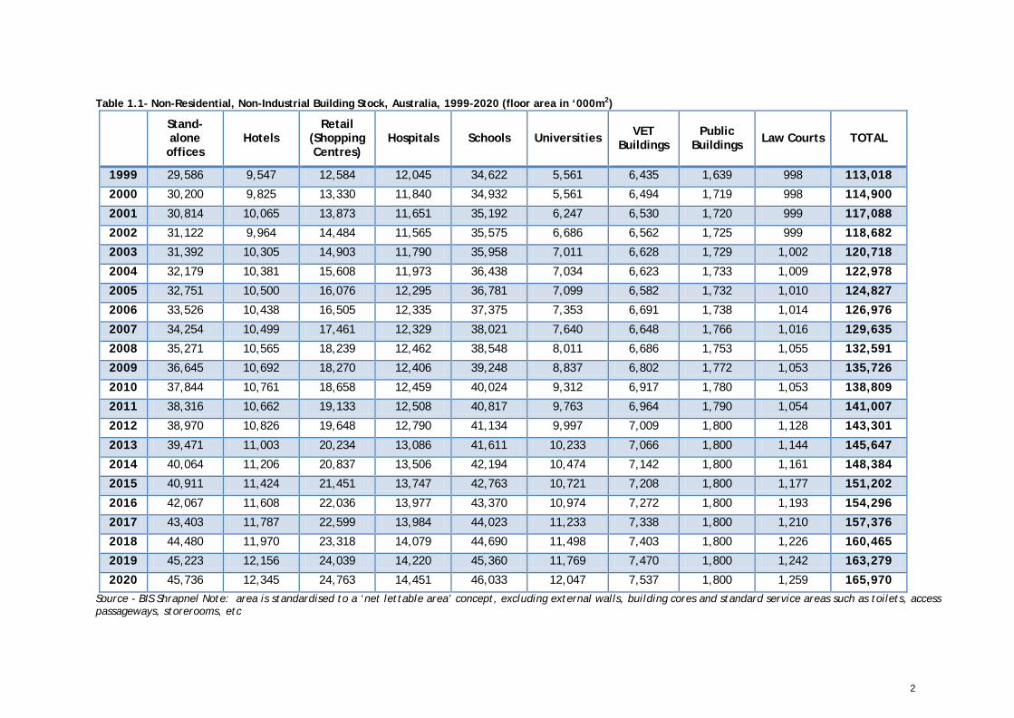
• Building Stock In 2009, the stock of commercial buildings that fall within the scope of this study amounted to just over 134 million m2 (see Table 1.1). A further 22 million m2 of ‘non-stand-alone’ office space was estimated to be in use in that same year (refer to Chapter 5 for details). The stock increased by 20% over the decade from 1999 and is projected to grow by a further 23% over the 11 years from 2009 to 2020. It should be noted that an attempt has been made to standardise area definitions to a ‘net lettable area’ (NLA), and in the case of retail buildings, gross lettable area-retail (GLAR). The difference between the Gross Floor Area and NLA of Buildings in the CBD could be as much as 25%.

1 Often referred to as ‘commercial buildings’, however in the building industry this phrase refers to buildings that are designed to earn a commercial rate of return on investment for their owners, whereas the set of buildings covered in this study includes many public buildings which do not share such an objective. 2 NFEE (2007), p. 13.

2

Table 1.1- Non-Residential, Non-Industrial Building Stock, Australia, 1999-2020 (floor area in ‘000m2)

Stand-alone offices

Hotels Retail

(Shopping Centres)

Hospitals Schools Universities VET Buildings

Public Buildings Law Courts TOTAL

1999 29,586 9,547 12,584 12,045 34,622 5,561 6,435 1,639 998 113,018

2000 30,200 9,825 13,330 11,840 34,932 5,561 6,494 1,719 998 114,900

2001 30,814 10,065 13,873 11,651 35,192 6,247 6,530 1,720 999 117,088

2002 31,122 9,964 14,484 11,565 35,575 6,686 6,562 1,725 999 118,682

2003 31,392 10,305 14,903 11,790 35,958 7,011 6,628 1,729 1,002 120,718

2004 32,179 10,381 15,608 11,973 36,438 7,034 6,623 1,733 1,009 122,978

2005 32,751 10,500 16,076 12,295 36,781 7,099 6,582 1,732 1,010 124,827

2006 33,526 10,438 16,505 12,335 37,375 7,353 6,691 1,738 1,014 126,976

2007 34,254 10,499 17,461 12,329 38,021 7,640 6,648 1,766 1,016 129,635

2008 35,271 10,565 18,239 12,462 38,548 8,011 6,686 1,753 1,055 132,591

2009 36,645 10,692 18,270 12,406 39,248 8,837 6,802 1,772 1,053 135,726

2010 37,844 10,761 18,658 12,459 40,024 9,312 6,917 1,780 1,053 138,809

2011 38,316 10,662 19,133 12,508 40,817 9,763 6,964 1,790 1,054 141,007

2012 38,970 10,826 19,648 12,790 41,134 9,997 7,009 1,800 1,128 143,301

2013 39,471 11,003 20,234 13,086 41,611 10,233 7,066 1,800 1,144 145,647

2014 40,064 11,206 20,837 13,506 42,194 10,474 7,142 1,800 1,161 148,384

2015 40,911 11,424 21,451 13,747 42,763 10,721 7,208 1,800 1,177 151,202

2016 42,067 11,608 22,036 13,977 43,370 10,974 7,272 1,800 1,193 154,296

2017 43,403 11,787 22,599 13,984 44,023 11,233 7,338 1,800 1,210 157,376

2018 44,480 11,970 23,318 14,079 44,690 11,498 7,403 1,800 1,226 160,465

2019 45,223 12,156 24,039 14,220 45,360 11,769 7,470 1,800 1,242 163,279

2020 45,736 12,345 24,763 14,451 46,033 12,047 7,537 1,800 1,259 165,970 Source - BIS Shrapnel Note: area is standardised to a ‘net lettable area’ concept, excluding external walls, building cores and standard service areas such as toilets, access passageways, storerooms, etc

3

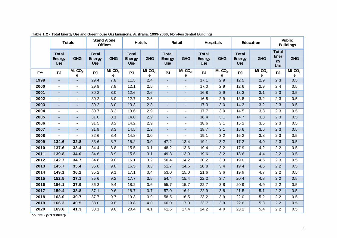
Table 1.2 - Total Energy Use and Greenhouse Gas Emissions: Australia, 1999-2000, Non-Residential Buildings

Totals Stand Alone Offices Hotels Retail Hospitals Education Public

Buildings

Total Energy

Use GHG

Total Energy

Use GHG

Total Energy

Use GHG

Total Energy

Use GHG

Total Energy

Use GHG

Total Energy

Use GHG

Total Energy

Use

GHG

FY: PJ Mt CO2-e PJ Mt CO2-

e PJ Mt CO2-e PJ Mt CO2-

e PJ Mt CO2-e PJ Mt CO2-

e PJ Mt CO2-e

1999 - - 29.4 7.8 11.5 2.4 - - 17.1 2.9 12.5 2.9 2.3 0.5

2000 - - 29.8 7.9 12.1 2.5 - - 17.0 2.9 12.6 2.9 2.4 0.5

2001 - - 30.2 8.0 12.6 2.6 - - 16.8 2.9 13.3 3.1 2.3 0.5

2002 - - 30.2 8.0 12.7 2.6 - - 16.8 2.9 13.8 3.2 2.3 0.5

2003 - - 30.2 8.0 13.3 2.8 - - 17.3 3.0 14.3 3.2 2.3 0.5

2004 - - 30.7 8.2 13.6 2.9 - - 17.7 3.0 14.5 3.3 2.3 0.5

2005 - - 31.0 8.1 14.0 2.9 - - 18.4 3.1 14.7 3.3 2.3 0.5

2006 - - 31.5 8.2 14.2 2.9 - - 18.6 3.1 15.2 3.5 2.3 0.5

2007 - - 31.9 8.3 14.5 2.9 - - 18.7 3.1 15.6 3.6 2.3 0.5

2008 - - 32.6 8.4 14.8 3.0 - - 19.1 3.2 16.2 3.8 2.3 0.5

2009 134.6 32.8 33.6 8.7 15.2 3.0 47.2 13.4 19.1 3.2 17.2 4.0 2.3 0.5

2010 137.6 33.4 34.4 8.8 15.5 3.1 48.2 13.6 19.4 3.2 17.9 4.2 2.2 0.5

2011 139.8 34.0 34.6 8.9 15.6 3.1 49.3 13.9 19.6 3.2 18.6 4.4 2.2 0.5

2012 142.7 34.7 34.8 9.0 16.1 3.2 50.4 14.2 20.2 3.3 19.0 4.5 2.3 0.5

2013 145.7 35.4 35.0 9.0 16.5 3.3 51.7 14.6 20.8 3.4 19.4 4.6 2.2 0.5

2014 149.1 36.2 35.2 9.1 17.1 3.4 53.0 15.0 21.6 3.6 19.9 4.7 2.2 0.5

2015 152.5 37.1 35.6 9.2 17.7 3.5 54.4 15.4 22.2 3.7 20.4 4.8 2.2 0.5

2016 156.1 37.9 36.3 9.4 18.2 3.6 55.7 15.7 22.7 3.8 20.9 4.9 2.2 0.5

2017 159.4 38.8 37.1 9.6 18.7 3.7 57.0 16.1 22.9 3.8 21.5 5.1 2.2 0.5

2018 163.0 39.7 37.7 9.7 19.3 3.9 58.5 16.5 23.2 3.9 22.0 5.2 2.2 0.5

2019 166.3 40.5 38.0 9.8 19.8 4.0 60.0 17.0 23.7 3.9 22.6 5.3 2.2 0.5

2020 169.6 41.3 38.1 9.8 20.4 4.1 61.6 17.4 24.2 4.0 23.2 5.4 2.2 0.5 Source - pitt&sherry

4

The modelled stock growth is a function of many factors, which vary between building types. These are described in chapters 5 to 11. However, a key underlying factor is the expectation of continued growth in Australia’s population and economy (see Section 3.6). Estimates of floor area per capita by building type are reported in the body of this Report. While there are variations by state and region in such calculations, they generally show consistent trends through time, providing a reasonable indicator of likely growth in the demand for floor area with a rising population. Other factors, such as changing population demographics, are also taken account, notably in the projections for hospital floor space (see Chapter 10 – Hospitals). For background on the stock model, please refer to Appendix C.

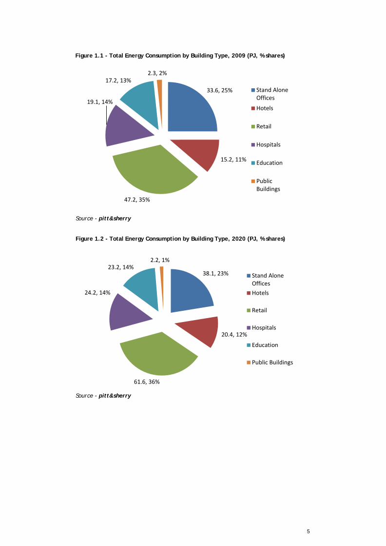
• Total Energy Consumption Total energy consumption3 in commercial buildings covered by this study is estimated to have been some 135 PJ in 2009, as shown in Table 1.2 above. This figure represents around 3.5% of the 3,907 PJ of gross final energy consumption in Australia in that year.4,5 Total energy consumption is expected to rise by 24% over the period 2009 to 2020, reaching just under 170 PJ by 2020. This reflects a combination of factors including a rising population, rising economic activity, a growing stock of commercial buildings and energy intensity trends that vary considerably by building type. Retail buildings accounted for the largest share of energy consumption in commercial buildings in 2009, consuming approximately 47 PJ or 35% of the total (see Figure 1.1). Office buildings represented the second largest share in 2009, with nearly 34 PJ or 25% of the total energy consumption. However, as discussed in Chapter 5, if ‘non-stand-alone’ offices are also considered, total energy consumption in offices in Australia could be significantly higher by approximately 26 PJ, and this would result in the total energy in all office building types in Australia above that of retail buildings. By 2020, the share of total energy consumption attributable to stand-alone offices is projected to fall to 23%, while retail’s share increases modestly (see Figure 1.2 below). This reflects the projection that energy intensity in offices may fall over the period to 2020, while growth in the office stock (25% by 2020 cf 2009) is slower than retail. By contrast, retail energy intensity is projected to increase, while at the same time as the retail stock grows more rapidly than offices (37% by 2020 cf 2009). The energy consumption shares attributable to other building types are expected to remain largely static. Expected growth in energy consumption by building type over the period from 2009 to 2020 is presented in Figure 1.3 below.

3 Note that all references to ‘energy consumption’ in this Report relate to the consumption of final energy sources, including electricity: conversion losses associated with the transformation of primary fuels into electricity are not included. 4 ABARES (2011), p. 17. 5 This figure is just under half that reported by ABARES for the total energy consumption of the ‘commercial and services’ sector of the economy in that year (287.4 PJ). However ABARES data includes energy consumption that is unrelated to buildings (such as transportation and process energy consumption), including significant energy using sectors such as waste water/sewage treatment. By contrast, this study only describes building-related energy use and does not cover all commercial building types. Appendix D provides further analysis of ‘top-down’ data, contrasting this with the bottom-up findings of this Report.

5

Figure 1.1 - Total Energy Consumption by Building Type, 2009 (PJ, % shares)

. Source - pitt&sherry

Figure 1.2 - Total Energy Consumption by Building Type, 2020 (PJ, % shares)

. Source - pitt&sherry

33.6, 25%

15.2, 11%

47.2, 35%

19.1, 14%

17.2, 13% 2.3, 2%

Stand AloneOffices

Hotels

Retail

Hospitals

Education

PublicBuildings

38.1, 23%

20.4, 12%

61.6, 36%

24.2, 14%

23.2, 14% 2.2, 1%

Stand AloneOfficesHotels

Retail

Hospitals

Education

Public Buildings

6

Figure 1.3 - Total Energy Consumption: Non-Residential, Non-Industrial Buildings, Australia,

2009 to 2020 (PJ)

Source - pitt&sherry

• Fuel Mix Electricity dominates the fuel mix for all commercial buildings in Australia, with a share of almost 83% in 2009 (see Figure 1.4 below). Given the relatively high average greenhouse gas intensity of electricity supply in Australia, this result largely explains why buildings exhibit a larger share of Australia’s greenhouse gas emissions than their share of energy use. Natural gas accounted for over 17% of the fuel mix in 2009, while LPG and diesel shares amounted to less than 1% in total. Figure 1.4 - Fuel Mix, All Buildings, 2009 (% shares)

. Source - pitt&sherry

0.0

20.0

40.0

60.0

80.0

100.0

120.0

140.0

160.0

180.0

2009

2010

2011

2012

2013

2014

2015

2016

2017

2018

2019

2020

Ener

gy (P

J)

Year

Public Buildings

Education

Hospitals

Retail

Hotels

Stand Alone Offices

82.4%

17.0%

0.6%

0.1%

Electricity

Gas

LPG

Diesel

7

While electricity is the dominant fuel (or energy source) for all the building types studied, the fuel mix does vary considerably by building type. Supermarkets, on average, use close to 100% electricity for their energy needs, while hospitals have the smallest electricity share, on average, at just over 49% in 2009 (balanced by a greater than 47% natural gas share).6 Offices are also electricity intensive, with an almost 90% electricity share in 2009, while shopping centres are similarly high at nearly 98% electricity. The fuel mix in offices has been largely static since 1999, with only a minor increase in the share of electricity at the expense of natural gas. Schools increased their share of electricity use on average from 72% in 1999 to more than 87% in 2009. Public buildings also increased their electricity use as a share of total energy, on average, from just under 60% in 1999 to a little over 70% by 2009, with natural gas shares falling in the same proportion. Looking forward to 2020, we expect the overall fuel mix across the stock of commercial buildings to be similar in 2020 as in the 2009 base year, with electricity continuing to hold around an 83% share of the fuel mix. Further analysis of the fuel mix by building type is provided in the Chapters 5-11. While a few of the data sets available to this study included records indicating use of GreenPower and/or on-site generation of renewable energy, there was insufficient data to draw statistically significant conclusions. Similarly, the data sets included no statistically significant information on the extent of cogeneration or trigeneration in buildings in Australia.

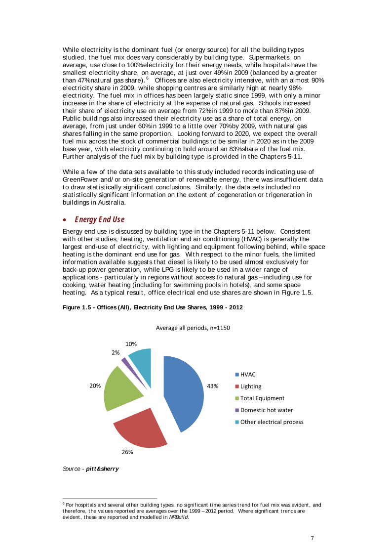
• Energy End Use Energy end use is discussed by building type in the Chapters 5-11 below. Consistent with other studies, heating, ventilation and air conditioning (HVAC) is generally the largest end-use of electricity, with lighting and equipment following behind, while space heating is the dominant end use for gas. With respect to the minor fuels, the limited information available suggests that diesel is likely to be used almost exclusively for back-up power generation, while LPG is likely to be used in a wider range of applications - particularly in regions without access to natural gas – including use for cooking, water heating (including for swimming pools in hotels), and some space heating. As a typical result, office electrical end use shares are shown in Figure 1.5. Figure 1.5 - Offices (All), Electricity End Use Shares, 1999 - 2012

. Source - pitt&sherry

6 For hospitals and several other building types, no significant time series trend for fuel mix was evident, and therefore, the values reported are averages over the 1999 – 2012 period. Where significant trends are evident, these are reported and modelled in NRBuild.

43%

26%

20%

2% 10%

Average all periods, n=1150

HVAC

Lighting

Total Equipment

Domestic hot water

Other electrical process

8

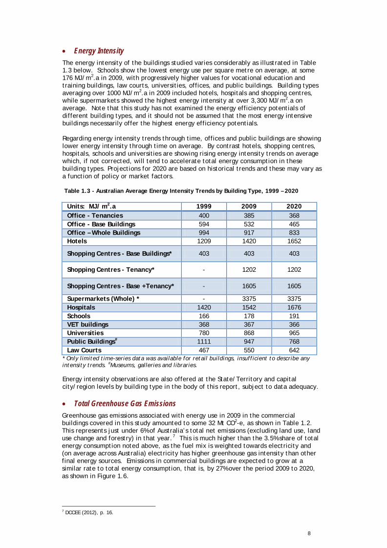
• Energy Intensity The energy intensity of the buildings studied varies considerably as illustrated in Table 1.3 below. Schools show the lowest energy use per square metre on average, at some 176 MJ/m2.a in 2009, with progressively higher values for vocational education and training buildings, law courts, universities, offices, and public buildings. Building types averaging over 1000 MJ/m2.a in 2009 included hotels, hospitals and shopping centres, while supermarkets showed the highest energy intensity at over 3,300 MJ/m2.a on average. Note that this study has not examined the energy efficiency potentials of different building types, and it should not be assumed that the most energy intensive buildings necessarily offer the highest energy efficiency potentials. Regarding energy intensity trends through time, offices and public buildings are showing lower energy intensity through time on average. By contrast hotels, shopping centres, hospitals, schools and universities are showing rising energy intensity trends on average which, if not corrected, will tend to accelerate total energy consumption in these building types. Projections for 2020 are based on historical trends and these may vary as a function of policy or market factors. Table 1.3 - Australian Average Energy Intensity Trends by Building Type, 1999 – 2020

Units: MJ/ m2.a 1999 2009 2020 Office - Tenancies 400 385 368 Office - Base Buildings 594 532 465 Office – Whole Buildings 994 917 833 Hotels 1209 1420 1652

Shopping Centres - Base Buildings* 403 403 403

Shopping Centres - Tenancy* - 1202 1202

Shopping Centres - Base +Tenancy* - 1605 1605

Supermarkets (Whole) * - 3375 3375 Hospitals 1420 1542 1676 Schools 166 178 191 VET buildings 368 367 366 Universities 780 868 965 Public Buildings# 1111 947 768 Law Courts 467 550 642

* Only limited time-series data was available for retail buildings, insufficient to describe any intensity trends. #Museums, galleries and libraries. Energy intensity observations are also offered at the State/Territory and capital city/region levels by building type in the body of this report, subject to data adequacy.

• Total Greenhouse Gas Emissions Greenhouse gas emissions associated with energy use in 2009 in the commercial buildings covered in this study amounted to some 32 Mt CO2-e, as shown in Table 1.2. This represents just under 6% of Australia’s total net emissions (excluding land use, land use change and forestry) in that year.7 This is much higher than the 3.5% share of total energy consumption noted above, as the fuel mix is weighted towards electricity and (on average across Australia) electricity has higher greenhouse gas intensity than other final energy sources. Emissions in commercial buildings are expected to grow at a similar rate to total energy consumption, that is, by 27% over the period 2009 to 2020, as shown in Figure 1.6.

7 DCCEE (2012), p. 16.

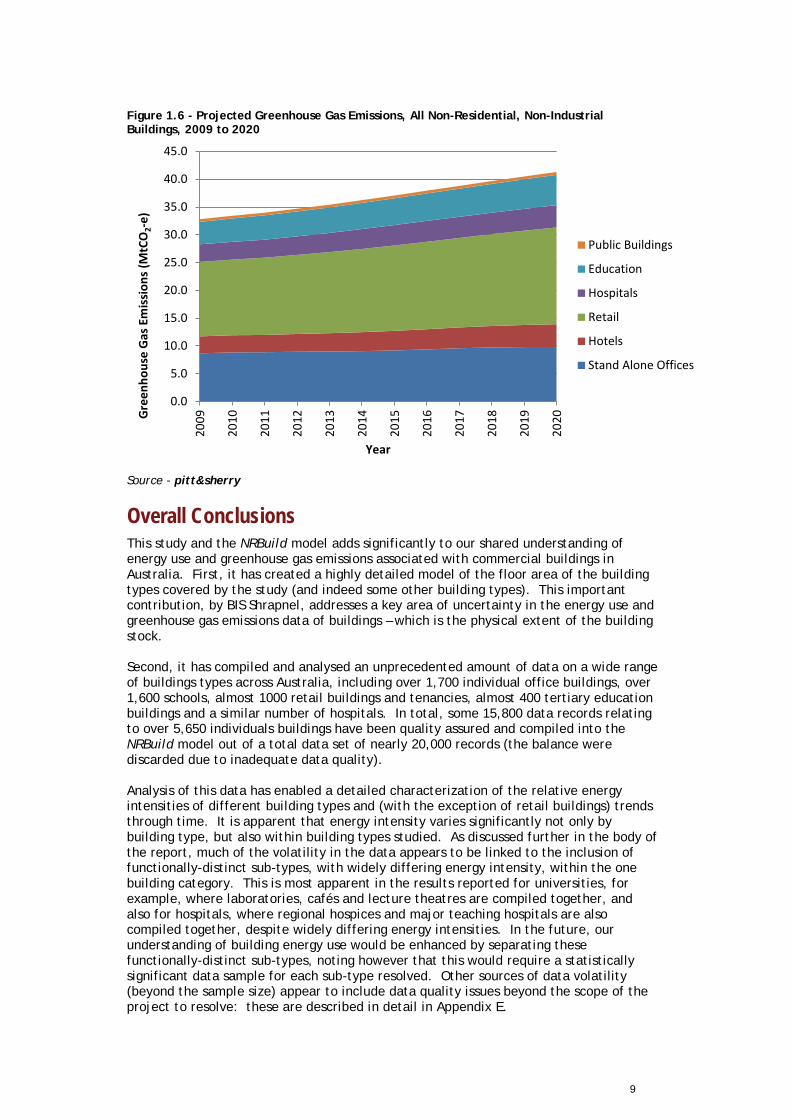
9

Figure 1.6 - Projected Greenhouse Gas Emissions, All Non-Residential, Non-Industrial Buildings, 2009 to 2020

Source - pitt&sherry

Overall Conclusions This study and the NRBuild model adds significantly to our shared understanding of energy use and greenhouse gas emissions associated with commercial buildings in Australia. First, it has created a highly detailed model of the floor area of the building types covered by the study (and indeed some other building types). This important contribution, by BIS Shrapnel, addresses a key area of uncertainty in the energy use and greenhouse gas emissions data of buildings – which is the physical extent of the building stock. Second, it has compiled and analysed an unprecedented amount of data on a wide range of buildings types across Australia, including over 1,700 individual office buildings, over 1,600 schools, almost 1000 retail buildings and tenancies, almost 400 tertiary education buildings and a similar number of hospitals. In total, some 15,800 data records relating to over 5,650 individuals buildings have been quality assured and compiled into the NRBuild model out of a total data set of nearly 20,000 records (the balance were discarded due to inadequate data quality). Analysis of this data has enabled a detailed characterization of the relative energy intensities of different building types and (with the exception of retail buildings) trends through time. It is apparent that energy intensity varies significantly not only by building type, but also within building types studied. As discussed further in the body of the report, much of the volatility in the data appears to be linked to the inclusion of functionally-distinct sub-types, with widely differing energy intensity, within the one building category. This is most apparent in the results reported for universities, for example, where laboratories, cafés and lecture theatres are compiled together, and also for hospitals, where regional hospices and major teaching hospitals are also compiled together, despite widely differing energy intensities. In the future, our understanding of building energy use would be enhanced by separating these functionally-distinct sub-types, noting however that this would require a statistically significant data sample for each sub-type resolved. Other sources of data volatility (beyond the sample size) appear to include data quality issues beyond the scope of the project to resolve: these are described in detail in Appendix E.

0.0

5.0

10.0

15.0

20.0

25.0

30.0

35.0

40.0

45.0

2009

2010

2011

2012

2013

2014

2015

2016

2017

2018

2019

2020G

reen

hous

e G

as E

mis

sion

s (M

tCO

2-e)

Year

Public Buildings

Education

Hospitals

Retail

Hotels

Stand Alone Offices

10

Despite the large amount of data compiled and analysed for this study, overall the data sample falls short of that required for statistically significant resolution of all of the building types and data fields set out in the terms of reference. The analytical ‘frame’ for this study (13 historical time periods, 15 geographical areas, 15 building sub-types, 2 ownership categories, 5 fuels, and up to 25 end-uses) demands some 730,000 unique and statistically significant observations. To achieve a confidence level of 95% that each of these observations is within 10% of the mean, a sample size of some 9700 building records would be required for each year. While the data collected for this study represents a substantial start on this task, the data records are unevenly distributed by year, region and building type. Very little historical data was available on retail buildings, for example, and these are amongst the most energy intensive of the commercial buildings studied. Also, the data set was too small to draw statistically significant conclusions about energy use trends at the sub-national level in most cases (although such conclusions are drawn where possible with respect to particular building types). Overall then, a key conclusion is that additional data capture and analysis is required for a complete analysis the building types covered in the terms of reference. At the same time, we note that some of the existing data limitations could be lifted with modest effort and cost, and without imposing any new reporting burdens, by measure such as:

• Improving data co-operation and sharing between agencies and levels of government in Australia

• Improving quality control in existing data collections and systems (such as OSCAR)

• Improving alignment between data owners with respect to key definitions and statistical concepts.

Also, data collection effort could be targeted to cover specific gaps in the existing data set. For example, a targeted data collection effort on the historical (1999 – 2010) energy consumption of retail buildings would enable a full description of that important building class. Similarly, for certain building types such as schools, the large overall data set includes almost census-like coverage of some states and territories and no data at all on others. A focused effort to capture the missing state/territory data would contribute much more to a statistically-significant picture than additional data collection in those states already well covered. Also, data collection effort could be prioritised towards those building types showing high and/or rising energy intensity and total energy consumption. These include supermarkets, other retail buildings, hospitals and hotels. By the same token, less effort would appear to be justified for schools, vocational education and training buildings and law courts.

11

2. Introduction 2.1 Background

This research was commissioned by the Australian Department of Climate Change and Energy Efficiency (DCCEE) as part of the joint Commonwealth, State and Territory work program under the National Strategy on Energy Efficiency (NSEE). The NSEE, which was approved by the Council of Australian Governments in July 2009, aims:

…to accelerate energy efficiency efforts, to streamline roles and responsibilities across levels of governments, and to help households and businesses prepare for the introduction of the Carbon Pollution Reduction Scheme.8

The NSEE is framed around four key themes:

1. Assisting households and businesses to transition to a low-carbon future

2. Reducing impediments to the uptake of energy efficiency

3. Making buildings more energy efficient

4. Government working in partnership and leading the way. Within the first theme, Measure 1.4.1 aims to “…improve data upon which national and jurisdictional energy efficiency policy development reporting and benchmarking can be based.”9 The work program to give effect this measure is known as the Energy Efficiency Data Project, which is managed by the Data Working Group (DWG) under the governance of Standing Council on Energy and Resources and chaired by the Federal Department of Resources, Energy and Tourism. The Energy Efficiency Data Project is aimed at:

…improving the evidence base for the development and evaluation of energy efficiency policies. The project will help achieve this by developing and implementing a plan for improving energy efficiency data collection and analysis, including methods to fill identified gaps. This will better inform the development, refinement and evaluation of new and existing energy efficiency policies.10

The Energy Efficiency Data Project comprises a range of data improvement projects, including this study (identified in its work program as ‘Activity E – Energy Use in Commercial Buildings’), which is managed by DCCEE. That Department issued a Request for Tender in October 2010, which was awarded in June 2011 to a consortium led by pitt&sherry in conjunction with major project partners Exergy Australia Pty Ltd and BIS Shrapnel, with peer review by the Sustainable Built Environment National Research Centre (see Section 2.4 - Project Team).

2.2 Project Objectives and Scope This research project involved the creation of a bottom-up model of energy use and greenhouse gas emissions associated with commercial buildings in Australia. Details on the methodology used to construct the model are provided in Appendix C. The model is known as NRBuild (Non-Residential Buildings) v.1.1, which has been developed for COAG and will be managed in the future by the DCCEE. The study period covers 1998-99 (financial year (FY) 1999) to 2019-20 (FY2020), with a ‘base year’ for model validation purposes of FY2009. 8 NSEE (2009), p. 4. 9 ibid, p. 13. 10 http://www.ret.gov.au/Documents/mce/energy-eff/nfee/committees/data/default.html , accessed 23 April 2012.

12

The building types/sub-types included are as follows:

• Offices (base buildings, tenancies, whole buildings)

• Hotels

• Shopping centres (base buildings, tenancies, whole buildings)

• Supermarkets (tenancies, whole buildings)

• Hospitals

• Schools

• TAFEs

• Universities

• Public buildings (incl. galleries, museums and libraries)

• Law courts

• Correctional centres. Building types not covered in this study include:

• Non-standalone offices

• Hotels and motels with fewer than 5 rooms

• Retail buildings outside enclosed shopping centres (other than supermarkets), including cafes, restaurants, pubs, clubs, retail shopping strips

• Health clinics and doctors’ surgeries

• Standalone aged care facilities

• Kindergartens/child care facilities

• Industrial buildings (including factories, warehouses, coolrooms and freezers)

• Data centres

• Laboratories (although some will be included under ‘Universities’)

• Religious buildings

• Transport-related buildings (airports, train stations, etc)

• All residential building types. The terms of reference for this study called for the stock and performance of privately-owned and government-owned offices, hospitals and educational buildings to be distinguished, and a separate report prepared. However, while some information is reported in the subsequent chapters, generally there was insufficient data on either the stock of these buildings by ownership type, or their energy performance, or both, to be able to draw significant conclusions. Similarly, while stock estimates for correctional centres are reported, there was insufficient data available to be able to characterise the energy performance of this stock and thus aggregate fuel consumption and greenhouse gas emissions are not estimated for this building type. For each of the building types studied, and for the period 1999 to 202011, this report estimates:

• Total energy consumption

• Energy consumption by base buildings and tenancies where relevant (offices, retail)

• Fuel consumption (electricity, natural gas, LPG and diesel)

• Renewable energy generation/consumption (where reported)

11 Data limitations prevented the estimation of historical values for retail buildings between 1999 and 2009.

13

• Energy end-use (where reported)

• Greenhouse gas emissions

• Floor area (and, in some cases, other ‘scale’ metrics such as hotel room numbers and hospital bed numbers).

These values were estimated nationally and for each state and territory, and also layered by capital cities and ‘regional’ (balance of state/territory). Some data records collected for this study contain additional fields beyond these ‘core’ requirements. The project outputs include:

1. This Report, summarising the key findings of the research and documenting the NRBuild model

2. The NRBuild model

3. A detailed building stock model constructed by BIS Shrapnel, which is incorporated in NRBuild in summary form.

2.3 Policy Context The need for improved data on energy use and efficiency in Australia has been recognised for some time. For example, in the Stage 2 Consultation Report that was released in 2007 under the National Framework on Energy Efficiency (NFEE) – the predecessor of the NSEE – it was noted:

Fundamental to the development and successful implementation of any new measures under the NFEE will be a comprehensive set of energy efficiency data. Currently energy efficiency data is limited, with little information available about energy use in important parts of the economy, for example commercial buildings.12

This sentiment was echoed more recently in the Report of the Prime Minister’s Task Group on Energy Efficiency, which states:

Without detailed information on what has worked or not in the past (and why), future actions are likely to be poorly targeted and wasteful. Innovation may be hindered because levels of uncertainty and risk are too high for investors. Without the capacity to track, analyse and project our energy efficiency performance we will not be able to measure progress towards national goals. This could result in substandard decisions about where to best invest limited public and private resources…

A large proportion of Australia’s low-cost abatement opportunities out to 2020 will involve unlocking opportunities in energy efficiency that are currently poorly understood. An effective framework of energy efficiency data and analysis to inform decisions and to target effort is essential.13

Finally this study - as the first comprehensive ‘baseline study’ that has been undertaken for the commercial buildings sector in Australia using primary data sources and analysis – is expected to contribute materially to a wider Energy Efficiency Data Framework in Australia. This Framework is being developed by the Australian, State and Territory Governments under the auspices of the Select Council on Climate Change, and in particular of the Data Working Group that reports ultimately to this Council.

2.4 The Project Team This study was undertaken by a consortium comprising:

12 NFEE (2007), p. 13. 13 DCCEE (2010), p. 84.

14

pitt&sherry • Phil Harrington, Principal Consultant – Climate Change, Project Manager

• Dr Hugh Saddler, Principal Consultant – Energy Strategies

• Dr Tony Marker, Senior Consultant – Building and Appliances

• Phil McLeod, Buildings Analyst

• Mark Johnston, Economist and Policy Analyst.

Exergy Australia Pty Ltd • Dr Paul Bannister, Director

• Chris Bloomfield, Director

• Alan Saunders, Project Manager

• Rosemary Barnes, Consultant

• Haibo Chen, Consultant

• Grace Foo, Consultant

• James Spears, Intern Energy Consultant.

BIS Shrapnel • Rob Mellor, Managing Director

• David Moore, Project Manager. The draft report and model findings were peer reviewed by:

Sustainable Built Environment National Research Centre • Dr Keith Hampson, Chief Executive Officer.

15

3. Overview of Methodology This section provides a brief overview of the methodology used in this research, and in particular the creation of the NRBuild model, version 1.1. For more details, please see Appendix C – Model Documentation. The high-level steps that were involved in this project can be summarised as follows:

1. Create a stock model of the relevant building types, by state, region, year and ownership type (where feasible and relevant)

• Backcast to 1999; forecast to 2020; validate model internally and externally

2. Capture and organise primary data on the energy performance of the relevant building types

• Data search/request; data compilation; data quality assurance

3. Undertake statistical analysis of energy data sets

• Create analytical ‘frame’ to match the required specifications (timeframe, spatial resolution, building sub-types, etc); regression analysis to establish trends through time for each sub-type; projections to 2020; compile sample size, standard deviations and other statistical indicators; end-use analysis;

4. Build an integrated stock and energy model

• Determine model functionality, user variables; integrate stock and energy/fuel intensities; calculate key outputs (energy use, greenhouse gas emissions) by year, region, building type and sub-type

5. Validate model

• Top-down analysis of energy consumption by fuel and building type; comparisons with other external research reports, independent data sources

6. Analyse and report findings. Schematically, this same process can be illustrated as shown in Figure 3.1 below.

3.1 Stock Model A bespoke stock model was created for this project by BIS Shrapnel, a firm with specialised expertise in analysis and forecasting in the construction sector. A building classification structure was developed, drawing largely on that used by the Australian Bureau of Statistics (ABS), which is based on the concept of the primary function of buildings. The primary metric used is floor space measured as ‘000m2 in terms of Net Lettable Area (NLA) or equivalent, except where otherwise specified. The data used to compile the estimate of commercial building stock is drawn from a wide array of different sources, with the different sources often not using a common definition of floor space. Adjustments have been made to some of the data provided in order that it approximates an NLA basis. Chapter 5 notes that there is considerable uncertainty surrounding floor area estimates in Australia.

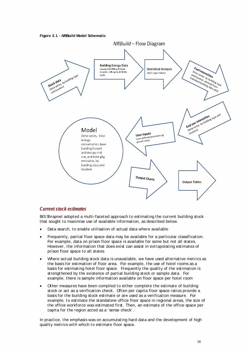
16

Figure 3.1 - NRBuild Model Schematic

Current stock estimates BIS Shrapnel adopted a multi-faceted approach to estimating the current building stock that sought to maximise use of available information, as described below.

• Data search, to enable utilisation of actual data where available

• Frequently, partial floor space data may be available for a particular classification. For example, data on prison floor space is available for some but not all states. However, the information that does exist can assist in extrapolating estimates of prison floor space to all states

• Where actual building stock data is unavailable, we have used alternative metrics as the basis for estimation of floor area. For example, the use of hotel rooms as a basis for estimating hotel floor space. Frequently the quality of the estimation is strengthened by the existence of partial building stock or sample data. For example, there is sample information available on floor space per hotel room

• Other measures have been compiled to either complete the estimate of building stock or act as a verification check. Often per capita floor space ratios provide a basis for the building stock estimate or are used as a verification measure. For example, to estimate the standalone office floor space in regional areas, the size of the office workforce was estimated first. Then, an estimate of the office space per capita for the region acted as a ‘sense check’.

In practice, the emphasis was on accumulating hard data and the development of high quality metrics with which to estimate floor space.

17

Historical stock estimates Backcasting the building stock is difficult and more imprecise than estimating the current building stock because of data limitations. The approach to backcasting the building stock was similar to that used to construct the estimates of the current building stock:

• Historical data was used where possible

• Classification metrics also provide a basis for backcasting data. For example, there is high quality historical data on the number of aged care places. This metric can be used as a basis for estimating floor space in historical periods. However, it is subject to the assumption that either the aged care place/floor space ratio is unchanged over time or can be estimated with reasonable accuracy

• Employment is a metric that can be used as a basis for estimating floor space and also for backcasting the stock estimates for some classifications. However, employment may be both volatile and cyclical. For this reason we have often smoothed the historical stock estimates when they have been derived from employment data or adjusted them to incorporate information from other sources such as building construction data or business numbers

• ABS building completion data can provide an insight into the pattern of changes in the building stock.

Forecast data The forecasts were based on a combination of existing BIS Shrapnel forecasts and more detailed sub-classification analysis. The intention was to forecast the underlying trend in floor space than cyclical ups and downs. The model also allows the easy input of alternative forecasts, either based on input of known projects or assumed percentage growth in floor space. The model provides a number of tailored ‘sense checks’ against which input forecasts can be checked. These vary between classifications, but normally include historical growth in floor space and also demographic benchmarks. Examples of the latter include retail floor space per capita, school floor space per school age person, prison floor space per prisoner. BIS Shrapnel has validated the building stock model through cross checking with other data sources and analysts, including further detailed comparisons with data from Geoscience Australia. However, we note that Geoscience Australia’s total stock estimates are significantly higher than ours, notwithstanding that the Geoscience model excludes hospitals and educational buildings. It is beyond the scope of this project to fully investigate this discrepancy.

3.2 Energy Consumption Data A feature of this study is that compiles a large amount of quality-assured primary data on actual building energy performance (along with some secondary data sources, as described below) to create a model of energy use in this sector. Some 20,000 records, each with up to 50 data fields (that is, up to 1 million data points) were initially compiled. With the quality assurance process described below, this number was reduced to some 15,800 records (relating to 5,650 individual buildings) that are utilised by the model (see Table 3.1). The number of records exceeds the number of individual buildings as some records relate to the same building in multiple time periods, while other records relate to tenancies within the same building. The sources of this data are described in more detail in Appendix D, but include:

• Energy audit data from Exergy Australia Pty Ltd, pitt&sherry and Energetics Pty Ltd

• NABERS ratings data provided by the NSW Office of Environment and Heritage

• Data provided directly by building owners and managers, including for numerous universities

18

• Data on government building energy use compiled in the OSCAR database14

• Data provided directly by government departments and agencies

• Public domain data from the public report of individual companies, institutions and industry associations.

An extensive quality assurance was conducted on these data inputs, as detailed in Appendix C. Despite this, in Chapter 3 – and in more detail in Appendix E – we note that there are still shortcomings in some of the data sets used in this study that have been beyond the scope of this study to address. Table 3.1 - Energy Data Records and Individual Building Counts by Building Type

Summary statistics on the building energy data used in the model:

Building type: Unique building count: Total record count:

Offices 1,715 4,308

Hotels 195 208

Retail 791 878

Retail - tenancies 261 1,102

Hospitals 352 972

Schools 1,641 6,475

Tertiary 385 1,274

Public buildings 28 235

Law courts 283 343

Totals 5,651 15,795 Source - pitt&sherry

Normalisation for Hours of Operation Where the data included significant information on operating hours (offices, retail), fuel use and energy use fields were normalised to the average hours of operation revealed in the relevant data set. For example, within retail tenancies, the data sets compiled for this study revealed mean values for operating hours per week of 59 for shopping centres and 96 for supermarkets15. Energy consumption by fuel and end-use was, therefore, factored for the deviation between the mean values and the actual, reported values for operating hours (the factor is described in the model as an ‘hour/s of operation energy intensity factor’). Records containing no information about operating hours were assumed to have the mean value and, therefore, not normalised. This normalisation process is important to be able to compare reported fuel and energy use intensity on a consistent basis with a building sub-type. A supermarket operating for 60 hours per week should use less energy than a supermarket operating for 120 hours per week, other things being equal. As discussed further in Appendix D, however, the 14 Online System for Comprehensive Activity Reporting. 15 Note that unweighted and area-weighted averages were compared, but differences between these values were typically small and therefore unweighted or simple averages were used for the normalisation process.

19

relationship between energy consumption and operating hours may not be linear, and in particular is less likely to be so as the value for hours of operation reaches extremes, due to the ‘fixed’ energy consumption of refrigeration, cool rooms, security lighting and other systems. Normalisations for other factors – such as climate – may also be relevant in certain circumstances. The NRBuild model is designed to facilitate a wide range of user investigations. For example, the ‘non-normalised’ energy data may be interrogated within the model, and the ‘energy intensity factor’ associated with hours of use may be varied by the user.16

3.3 Data Analysis and Model Construction The energy data sets were analysed according to the analytical ‘frame’ required for this study; that is, by building type and sub-type, ownership type (offices), year (data records covered the period 1999 to 2012), state and territory, region (capital city vs regional, or balance of state, with ACT treated a ‘capital city’ only). As discussed in Section 3.5 below, this analytical frame requires around 730,000 statistically valid observations to be fully populated and therefore completely resolved. For each combination of building type, ownership type, state, region and year, observations were calculated from the data sets regarding the intensity of use of individual fuels (electricity, gas, LPG, diesel and renewables, where revealed, or ‘total energy’, where fuel use is not revealed). Each observation is associated with the sample size (the number of separate records used) relied upon for that observation. A tool is provided within the model that enables the user to specify the minimum sample size per observation, with all values that fall below that sample size being eliminated from the analysis. This provides an initial tool for the model user to test and visualise the robustness of each analysis. The next step was to construct time-series analyses, including backcasting to 1999 and forecasting to 2020. For each building sub-type, a regression analysis was performed on at least the average national energy intensity time series, as this provided the largest data sample. In some cases, there was sufficient information on fuel mix changes through time to also be able to perform regression analyses. We note that regression analyses could be performed on many other parameters within model. The model includes a tool which enables the user to specify the minimum sample size relied upon for regression analyses. Generally, simple linear regressions provided adequate interpretation of data trends, although this varied greatly by building type and sub-type, as reported on in the relevant chapters below. The model then captures fitted trends in energy intensity and fuel mix over time, by building sub-type, with the stock trends for that building-type, to estimate the evolution of total fuel use, and hence greenhouse gas emissions over time. The model aims to balances ease of use with flexibility, to cater for a range of uses and users with different requirements and skill levels. Default values for all key variables are calculated from the data sets as described above, together with other factors such as the greenhouse gas intensity of electricity supply by state through time, and these are used to populate summary tables of energy use and greenhouse gas emissions. At the same time, more advanced users, or users with particular research needs, may substitute their own assumptions for key variables in order to understand the effect of these assumptions on energy use and/or emissions. This feature is limited to years after the ‘base year’ (FY2009), to ensure that historical values are not changed. The user-specifiable values (for each building sub-type) include:

• Greenhouse gas intensity of electricity supply by state by year

• Average energy intensity by year

• Fuel mix by year (including Green Power/onsite renewables share)

• Stock growth by year

16 Subject to confidentiality constraints.

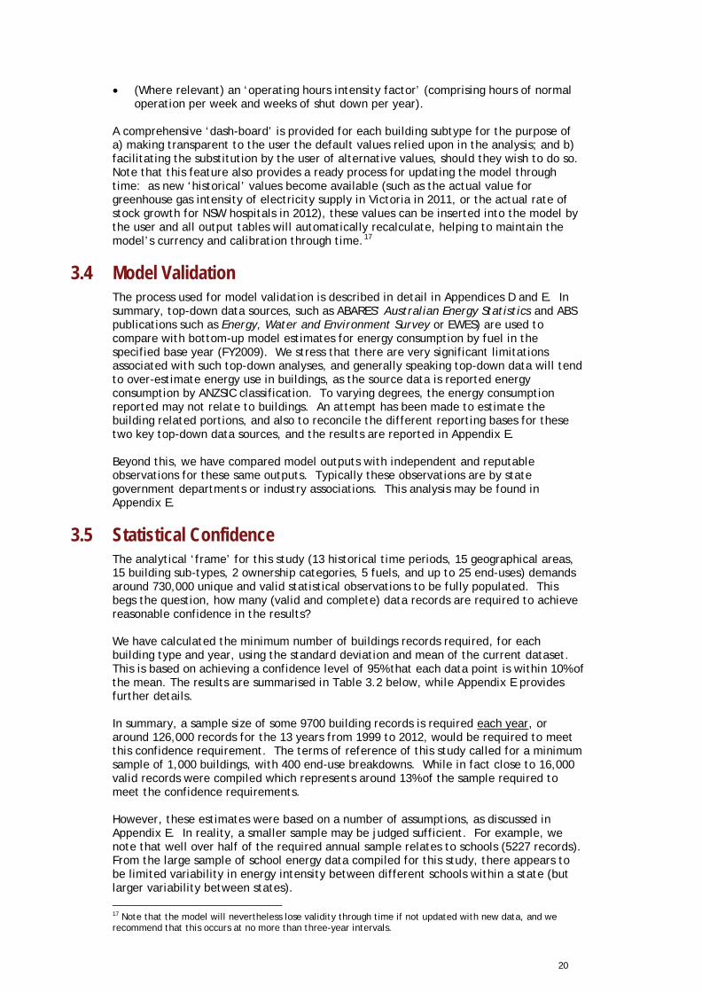
20

• (Where relevant) an ‘operating hours intensity factor’ (comprising hours of normal operation per week and weeks of shut down per year).

A comprehensive ‘dash-board’ is provided for each building subtype for the purpose of a) making transparent to the user the default values relied upon in the analysis; and b) facilitating the substitution by the user of alternative values, should they wish to do so. Note that this feature also provides a ready process for updating the model through time: as new ‘historical’ values become available (such as the actual value for greenhouse gas intensity of electricity supply in Victoria in 2011, or the actual rate of stock growth for NSW hospitals in 2012), these values can be inserted into the model by the user and all output tables will automatically recalculate, helping to maintain the model’s currency and calibration through time.17

3.4 Model Validation The process used for model validation is described in detail in Appendices D and E. In summary, top-down data sources, such as ABARES’ Australian Energy Statistics and ABS publications such as Energy, Water and Environment Survey or EWES) are used to compare with bottom-up model estimates for energy consumption by fuel in the specified base year (FY2009). We stress that there are very significant limitations associated with such top-down analyses, and generally speaking top-down data will tend to over-estimate energy use in buildings, as the source data is reported energy consumption by ANZSIC classification. To varying degrees, the energy consumption reported may not relate to buildings. An attempt has been made to estimate the building related portions, and also to reconcile the different reporting bases for these two key top-down data sources, and the results are reported in Appendix E. Beyond this, we have compared model outputs with independent and reputable observations for these same outputs. Typically these observations are by state government departments or industry associations. This analysis may be found in Appendix E.

3.5 Statistical Confidence The analytical ‘frame’ for this study (13 historical time periods, 15 geographical areas, 15 building sub-types, 2 ownership categories, 5 fuels, and up to 25 end-uses) demands around 730,000 unique and valid statistical observations to be fully populated. This begs the question, how many (valid and complete) data records are required to achieve reasonable confidence in the results? We have calculated the minimum number of buildings records required, for each building type and year, using the standard deviation and mean of the current dataset. This is based on achieving a confidence level of 95% that each data point is within 10% of the mean. The results are summarised in Table 3.2 below, while Appendix E provides further details. In summary, a sample size of some 9700 building records is required each year, or around 126,000 records for the 13 years from 1999 to 2012, would be required to meet this confidence requirement. The terms of reference of this study called for a minimum sample of 1,000 buildings, with 400 end-use breakdowns. While in fact close to 16,000 valid records were compiled which represents around 13% of the sample required to meet the confidence requirements. However, these estimates were based on a number of assumptions, as discussed in Appendix E. In reality, a smaller sample may be judged sufficient. For example, we note that well over half of the required annual sample relates to schools (5227 records). From the large sample of school energy data compiled for this study, there appears to be limited variability in energy intensity between different schools within a state (but larger variability between states). 17 Note that the model will nevertheless lose validity through time if not updated with new data, and we recommend that this occurs at no more than three-year intervals.

21

Therefore, it may suffice to compile a smaller data set for each state, but ensure that all states are covered (the current data set has no coverage of TAS, VIC, WA or SA). Also, annual data may not be required to establish valid time series trends; data points every three years may suffice. Table 3.2 – Recommended Minimum Sample Sizes per Year

Minimum sample size, per year

Offices 1508 Hotels 540 Hospitals 258 Schools 5227 University Buildings 679 VET Buildings 181 Shopping Centres 692 Supermarkets 319 Public Buildings 106 Law Courts 154 TOTAL AUSTRALIA 9664

Source – pitt&sherry/Exergy Australia. Assuming 13 regions are resolved with 95% confidence level and a 10% standard error and a finite population.

3.6 Key Assumptions

3.6.1 Greenhouse Gas Intensity of Electricity Supply An important assumption underpinning the greenhouse gas emissions projections is the greenhouse gas intensity of electricity supply. This varies widely by state and, in some cases, has also changed significantly in the period since 1999. The future path of this variable is highly uncertain, particularly at a state level. Some projections for Australia as a whole are contained in the Treasury modelling of the carbon pricing scheme.18 However these are not broken down by state. Also, there is increasing interconnection of states (at least from SA to Qld) and interstate trading of electricity within the National Energy Market (NEM), which is increasingly blurring the unique state-based greenhouse ‘signatures’ through time. As a result of this uncertainty, the NRBuild model makes the conservative assumption of no change in the 2010 values for greenhouse gas intensity of electricity supply by state out to 2020 (see Figure 3.2). However, these variables may be altered by the model user and unique values specified by year for each state and territory if desired. The greenhouse gas intensity of other fuels has been sourced from the National Greenhouse Accounts Factors Workbook 2011 and these are assumed to remain unchanged through to 2020.19

18 Federal Treasury (2011). 19 DCCEE (2011).

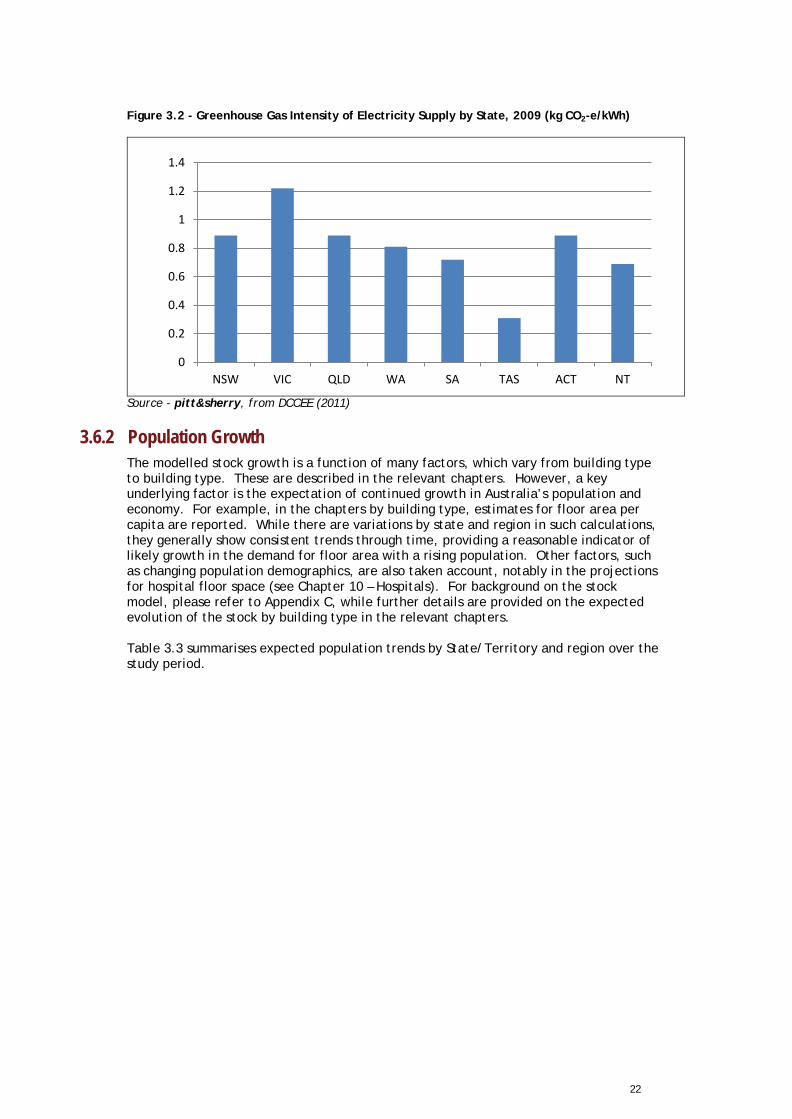
22

Figure 3.2 - Greenhouse Gas Intensity of Electricity Supply by State, 2009 (kg CO2-e/kWh)

Source - pitt&sherry, from DCCEE (2011)

3.6.2 Population Growth The modelled stock growth is a function of many factors, which vary from building type to building type. These are described in the relevant chapters. However, a key underlying factor is the expectation of continued growth in Australia’s population and economy. For example, in the chapters by building type, estimates for floor area per capita are reported. While there are variations by state and region in such calculations, they generally show consistent trends through time, providing a reasonable indicator of likely growth in the demand for floor area with a rising population. Other factors, such as changing population demographics, are also taken account, notably in the projections for hospital floor space (see Chapter 10 – Hospitals). For background on the stock model, please refer to Appendix C, while further details are provided on the expected evolution of the stock by building type in the relevant chapters. Table 3.3 summarises expected population trends by State/Territory and region over the study period.

0

0.2

0.4

0.6

0.8

1

1.2

1.4

NSW VIC QLD WA SA TAS ACT NT

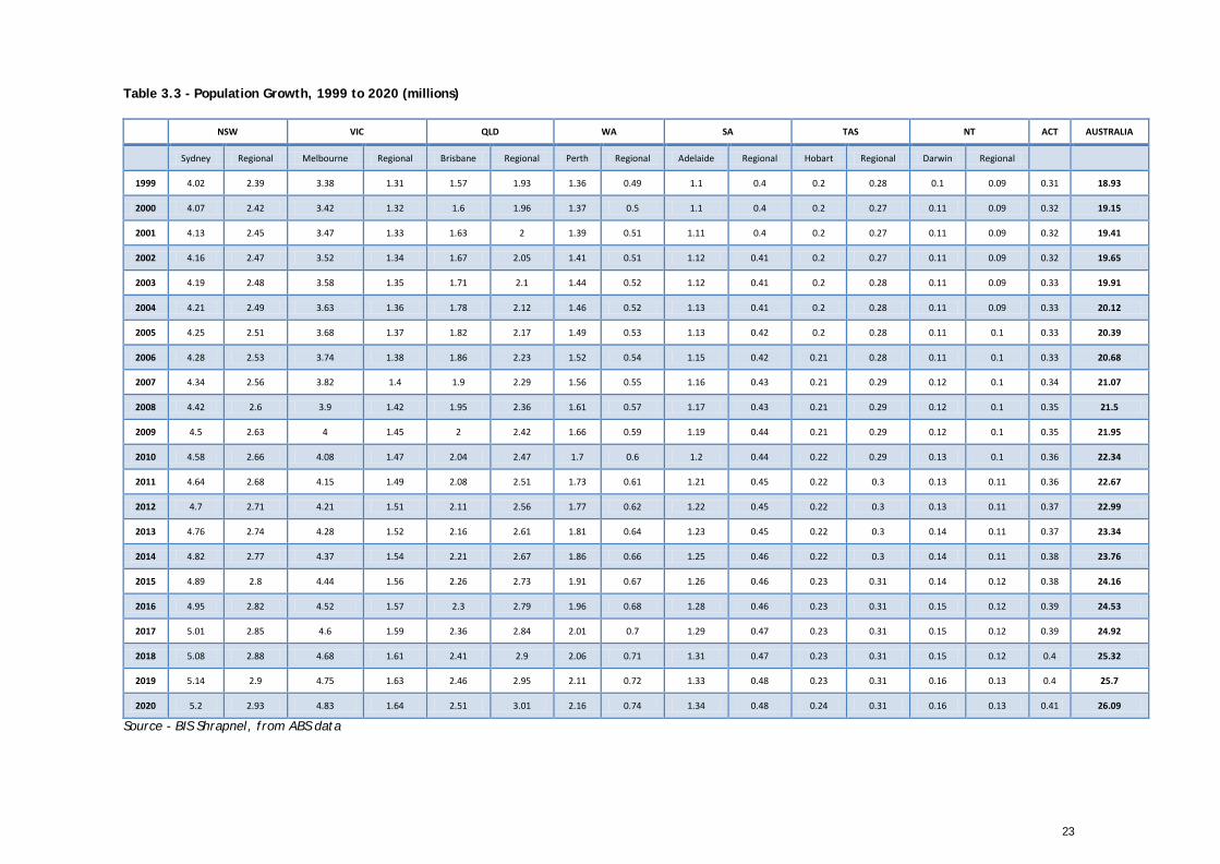
23

Table 3.3 - Population Growth, 1999 to 2020 (millions)

NSW VIC QLD WA SA TAS NT ACT AUSTRALIA

Sydney Regional Melbourne Regional Brisbane Regional Perth Regional Adelaide Regional Hobart Regional Darwin Regional

1999 4.02 2.39 3.38 1.31 1.57 1.93 1.36 0.49 1.1 0.4 0.2 0.28 0.1 0.09 0.31 18.93

2000 4.07 2.42 3.42 1.32 1.6 1.96 1.37 0.5 1.1 0.4 0.2 0.27 0.11 0.09 0.32 19.15

2001 4.13 2.45 3.47 1.33 1.63 2 1.39 0.51 1.11 0.4 0.2 0.27 0.11 0.09 0.32 19.41

2002 4.16 2.47 3.52 1.34 1.67 2.05 1.41 0.51 1.12 0.41 0.2 0.27 0.11 0.09 0.32 19.65

2003 4.19 2.48 3.58 1.35 1.71 2.1 1.44 0.52 1.12 0.41 0.2 0.28 0.11 0.09 0.33 19.91

2004 4.21 2.49 3.63 1.36 1.78 2.12 1.46 0.52 1.13 0.41 0.2 0.28 0.11 0.09 0.33 20.12

2005 4.25 2.51 3.68 1.37 1.82 2.17 1.49 0.53 1.13 0.42 0.2 0.28 0.11 0.1 0.33 20.39

2006 4.28 2.53 3.74 1.38 1.86 2.23 1.52 0.54 1.15 0.42 0.21 0.28 0.11 0.1 0.33 20.68

2007 4.34 2.56 3.82 1.4 1.9 2.29 1.56 0.55 1.16 0.43 0.21 0.29 0.12 0.1 0.34 21.07

2008 4.42 2.6 3.9 1.42 1.95 2.36 1.61 0.57 1.17 0.43 0.21 0.29 0.12 0.1 0.35 21.5

2009 4.5 2.63 4 1.45 2 2.42 1.66 0.59 1.19 0.44 0.21 0.29 0.12 0.1 0.35 21.95

2010 4.58 2.66 4.08 1.47 2.04 2.47 1.7 0.6 1.2 0.44 0.22 0.29 0.13 0.1 0.36 22.34

2011 4.64 2.68 4.15 1.49 2.08 2.51 1.73 0.61 1.21 0.45 0.22 0.3 0.13 0.11 0.36 22.67

2012 4.7 2.71 4.21 1.51 2.11 2.56 1.77 0.62 1.22 0.45 0.22 0.3 0.13 0.11 0.37 22.99

2013 4.76 2.74 4.28 1.52 2.16 2.61 1.81 0.64 1.23 0.45 0.22 0.3 0.14 0.11 0.37 23.34

2014 4.82 2.77 4.37 1.54 2.21 2.67 1.86 0.66 1.25 0.46 0.22 0.3 0.14 0.11 0.38 23.76

2015 4.89 2.8 4.44 1.56 2.26 2.73 1.91 0.67 1.26 0.46 0.23 0.31 0.14 0.12 0.38 24.16

2016 4.95 2.82 4.52 1.57 2.3 2.79 1.96 0.68 1.28 0.46 0.23 0.31 0.15 0.12 0.39 24.53

2017 5.01 2.85 4.6 1.59 2.36 2.84 2.01 0.7 1.29 0.47 0.23 0.31 0.15 0.12 0.39 24.92

2018 5.08 2.88 4.68 1.61 2.41 2.9 2.06 0.71 1.31 0.47 0.23 0.31 0.15 0.12 0.4 25.32

2019 5.14 2.9 4.75 1.63 2.46 2.95 2.11 0.72 1.33 0.48 0.23 0.31 0.16 0.13 0.4 25.7

2020 5.2 2.93 4.83 1.64 2.51 3.01 2.16 0.74 1.34 0.48 0.24 0.31 0.16 0.13 0.41 26.09

Source - BIS Shrapnel, from ABS data

24

4. Key Issues A full understanding of the energy consumption of commercial buildings in Australia requires adequate knowledge of at least five key parameters:

1. The structure of the sector (i.e., its physical nature including building numbers, total area, location, number of floors, etc; the fuel mix within the sector; the stock and nature of end use equipment such as lighting equipment, space conditioning equipment, etc; operational requirements and settings such as temperature set-points, ventilation rates, minimum lighting levels, etc)

2. Activity levels within the sector (the intensity of use of buildings, such as hours of operation, visitor or staff numbers, hospital bed numbers and separations, etc; and the intensity of use of end-use equipment within buildings)

3. The energy intensity of fuel use (fuel use per unit of structure or activity)

4. Explanatory factors (a wide range of variables that may help interpret observed trends, including climate data, energy prices)

5. The inter-relationships between these factors, so that causality can be established (for example, it may be revealed that larger hospitals use more energy per unit area than smaller hospitals, but is this because they have a higher turnover of patients, more patients per unit floor area, more medical equipment and higher rates of usage of such equipment, higher service levels (like temperature set points, lighting levels), or some combination of these factors.

However as noted in Chapter 3, there is a significant shortage of reliable, comprehensive and spatially disaggregated data in the public domain with respect to energy consumption and end use, correlated with activity levels and the structural composition of the built environment in Australia. While this study goes some way towards addressing this shortage, it represents a one-off study, which is not a substitute for an ongoing statistical data collection and analysis process. This chapter reviews the key issues, including uncertainties, in some detail. It covers issues with respect to:

1. The building stock

2. Energy performance data

3. The NRBuild model scope and resolution.

4.1 The Building Stock The aim of this study is to understand energy use in commercial and associated greenhouse gas emissions, in particular by building up ‘bottom up’ model of the intensity of energy use in different building types. However, a key and prior issue is the very considerable uncertainty that surrounds the nature and extent of the physical stock of buildings in Australia. There is no single or authoritative source that can be referred to in order to answer key questions such as:

• How many commercial buildings are there in Australia?

• How many square metres of commercial buildings are there?

• What is the break-down of the stock by function, size, age, location, ownership, tenancy or other key parameters?

• How are these parameters changing through time? Similarly, there is very limited information on the intensity of use of buildings (eg, hours of operation, building occupancy levels, occupant behaviours, etc), and yet these usage patterns will affect energy consumption in a significant manner.

25

The Australian Bureau of Statistics (ABS) conducts certain surveys including Building Approvals, Australia (ABS 2011a), Building Activity, Australia (ABS 2011b) and Construction Work Done, Australia, Preliminary (ABS 2011c). The building activity survey covers the value of construction of new buildings and alterations and additions to existing buildings. However, no data is captured (or at least published) on the physical result of this expenditure, such as a change in the number, area or quality of buildings comprising the extant building stock. For example, the flows of expenditure recorded may relate to the creation of new stock, the refurbishment of existing stock or even the demolition of stock. As a result, the ABS value of construction data cannot be used directly to estimate the building stock through time. It does, however, provide a validation source for estimates produced from other primary sources. The ABS also produces a range of data series which can be useful to support analysis of energy consumption and as a tool to either provide a proxy or a verification of the estimate of the building stock. For example, it produces a series on the number of hotel rooms,20 which is a useful analytical tool in its own right as well as being indicative of the floor area stock of hotels. The Property Council of Australia (PCA) and BIS Shrapnel both maintain important data sets with respect to commercial office buildings. PCA’s Office Market Report (available commercially online) covers approximately 4,500 office buildings in over 30 office markets around Australia, including historical data since January 1990 for total stock, vacancy, supply, withdrawals and net absorption, with a comprehensive list of future supply and development details. The spatial coverage of the model is wide, covering all central business districts and 17 regional centres, but it does not cover the whole of Australia. Other companies including property developers and managers, and bodies such as the Real Estate Institute of Australia (REIQ), the Facility Management Association (FMA), the Construction Forecasting Council and many others are likely to hold relevant data. However, such data are not always available in the public domain. For hospitals, the Institute of Health and Welfare maintains the ‘Australian hospital statistics’ series (AIHW 2011).

4.1.1 Building Stock Structure and Turnover For many policy applications, it is essential to understand factors such as:

• The rate of entry of new buildings into the stock

• The rate of demolition of existing buildings in the stock

• The extent of ‘major refurbishment’ of the existing stock, for example, a level of refurbishment sufficient to trigger the application of the current version of the Building Code of Australia

• The number of buildings by size, type and location

• The age profile of the stock (or distribution by ‘vintage’ year). At present, there are no statistical collections in the public domain that bear directly upon such questions. As a result, the stock model constructed for this study does not explicitly represent stock turnover, but rather the total stock in each time period. That is, the stock model is not able to be layered by the age or ‘vintage’ of the buildings, or to separately represent additions, refurbishments and retirements. Further, it estimates total floor area by building type, rather than building numbers layered by building size. Depending upon the context, both of these would be useful.

4.1.2 Floor Area Definitions A key uncertainty for the estimation of the floor area of commercial buildings in Australia – and hence for their energy intensity – is the inconsistent application of floor

20 ABS Catalogue 8635.0, Tourist Accommodation, Australia, Dec 2011.

26

area definitions in different data sets. Numerous floor area concepts are in use in Australia, with sectors (such as retail, commercial, education, hospitals) tending to use similar concepts within their sector21. However, depending upon the data source, it is very common that the conceptual basis of floor area estimates varies between building type and source, is inconsistently applied, or is simply unstated. Most of the OSCAR data sets relating to government owned or occupied buildings, including offices, hospitals, schools and tertiary buildings fall into this category. As there may be a 25% difference in floor area (m2) between a net lettable area (NLA) concept and a gross floor area (GFA) concept, this may introduce up to 25% error in energy intensity and, potentially, total energy consumption, estimates. In principle, this error could be eliminated if both the area estimation and the energy intensity estimation are conducted using the same conceptual construct for area. However, in practice, both the underlying data sources used for the stock model in this study, and many of the energy data records, are ambiguous on this key point. BIS Shrapnel has attempted to standardise all floor area estimates to a NLA basis, or approximate equivalent. This may tend to understate total energy consumption in the non-retail sectors as reported in this study. The differences in sources and definitions of data accessed by BIS Shrapnel also mean that inter-state and intra-state comparisons of floor space should be treated with caution. Although BIS Shrapnel has attempted to normalise the data, the normalisation process is only approximate.

4.2 Energy Performance Data Statistical information about energy consumption in Australia is collected through three primary processes. First, enterprises that consume at least 200 TJ of energy per year are required to report their consumption under the mandatory National Greenhouse and Energy Reporting (NGERS) legislation. NGERS is managed by the Clean Energy Regulator. This reporting process covers around 700 major enterprises involved in energy production, transformation or consumption, and is limited to controlling corporations that produce or consume at least 200 TJ of energy or individual sites that produce or consume 100 TJ. It is estimated that NGERS captures data on around 90% of Australia’s total energy consumption, although this energy is consumed by just 0.1% of Australia’s business enterprises.22 That is, it captures no data on the 99.9% of businesses that consume less that 200 TJ per year. Many sectors of the economy are likely to be wholly or largely absent from NGERS energy consumption data, with examples including agriculture, fishing and forestry; public administration and safety; administrative and support services; and education and training inter alia. It captures no data on the energy consumption of non-incorporated entities, which may include charities and other organisations that occupy commercial buildings. NGERS also does not capture any information on energy end-use, for example, what portion of the total energy consumption reported is associated with buildings.

Second, the ABS has recently commenced a new survey, the Energy, Water and Environment Survey (EWES) (ABS Publication 4660.0 - Energy, Water and Environment Management, 2008-09) which was sent to some 14,000 Australian businesses23. This publication was released for the first time in 2011 and is expected to be repeated at least every three years. This publication contains estimates of energy expenditure and usage by Australian businesses for 2008-09 inter alia. EWES provides valuable data on enterprise numbers, expenditure on fuels, fuel use by enterprise size and other parameters, for a number of sectors that may be defined, at least partially, as ‘commercial’. These sectors (and their relevant ANZSIC division code) include:

21 See, for example, the online publication, Property Council of Australia (PCA) Method of Measurement (A Summary), athttp://www.unisanet.unisa.edu.au/staff/peterrossini/Basic_Property_Resources.htm?http://www.unisanet.unisa.edu.au/staff/peterrossini/Basic_Property_Resources/Property%20Council%20of%20Australia%20(PCA)%20Method%20of%20Measurement%20(A%20Summary).htm accessed on 3 May 2012. 22 Personal communication with ABARES. 23 http://www.abs.gov.au/AUSSTATS/abs@.nsf/Lookup/4660.0Explanatory%20Notes12008-09?OpenDocument#PARALINK7

27

• Wholesale trade (Division F)

• Retail trade (Division G)

• Accommodation and food services (Division H)

• Information media and telecommunications (Division J)

• Auxiliary finance and insurance services (parts of Division K)

• Rental hiring and real estate services (Division L)

• Administrative and support services (Division N)

• Public order safety and regulatory services (Division O)

• Arts and recreation services (Division R)

• Other services (Division S).

However, the survey excludes certain sectors, many of which fall into the scope of this study, including:

• Agriculture

• Water Supply, Sewerage and Drainage Services

• Finance

• Insurance

• Public Administration

• Defence

• Private Households Employing Staff

• General Government.

Also, no information is available from this source on energy end use, and this prevents accurate disaggregation of total energy consumption within these sectors into that associated with commercial buildings (or end uses within those buildings), as distinct from other energy uses including transportation and process energy use. Nevertheless EWES helps to fill a gap left by NGERS, and that is coverage of the energy consumption of the very large number of smaller energy users in Australia. BREE therefore uses both the NGER and EWES data in a range of statistical techniques to estimate total consumption, which is validated in its energy balance process. In a third key process, ABARES/BREE produce each year the Australian Energy Statistics (AES). AES provides data on total annual energy consumption in ‘commercial and services’ sector, inter alia, by State and by fuel (ABARES 2011). AES draws on a wide range of primary data sources, chief of which is NGERS (replacing its own Fuel and Electricity Survey), and sector-specific surveys or data sources. However, the limitations of the AES for this study include that the data is not broken down by ANZSIC Division or enterprise, and does not reveal the portion of energy consumption attributable to energy use in commercial buildings (as distinct from other aspects of the operations of entities in the sector). No end-use information is available from this source. Importantly, however, AES is prepared following a full energy balance process that reconciles energy production, trade and intermediate and final consumption, which means that its aggregate values for energy consumption are robust. Beyond these data sources, there are a number of other data sources that provide some insights into building energy use. For example the Energy Efficiency Opportunities (EEO) program requires entities that consume more than 0.5 PJ (500 TJ) of energy annually to assess and report efficiency opportunities. Some of these entities will have energy consumption that is largely associated with commercial buildings (eg, banks, property groups, retailers). Indeed, it is estimated that some 25% of energy use in the

28

services sector is attributable to companies that report under EEO24. However, only aggregate national consumption by EEO companies is reported and no detailed end use or activity data (e.g. m2 of buildings) is published. Nevertheless, some individual EEO companies voluntarily reports additional information. An important data set has been compiled over time in NABERS, the National Australian Built Environment Rating System. A database of all assessments performed under NABERS has been compiled covering a range of building types including offices, hotels, and retail shopping centres (with others under development). Some of this data has been accessed for this project. For further information on the data sources used for this study, please refer to Appendix C.

4.2.1 Energy End Use by Building Type Within the overall paucity of statistical information on building energy performance, a particular gap is that there is no regular statistical collection that identifies the nature of energy end use in the commercial buildings sector. This contrasts greatly with the relatively rich understanding of energy end-use in residential buildings, resulting from numerous and regular ABS data collections25, along with detailed data on the stock and efficiency of new appliances resulting from the national minimum energy performance standards and labelling program. This study has compiled over 400 end-use breakdowns. However, given the large number of years, regions and building types covered in this study and resolved in the NRBuild model, this has proven sufficient only for broad averages to be compiled for end use for some building types, and none at all for some fuels and building types. A well targeted data survey focusing on energy end use could fill this knowledge gap, allowing greater resolution within the model and greater utility for policy analysis.

4.2.2 Data Quality While the data compiled for this study has been extensively quality assured, as described in Appendix C, to remove obvious errors, some data sources exhibit signs of bias or error that were beyond the scope of this research to resolve. In Appendix E we provide a formal statistical analysis of the compiled data sets. We note in particular that generally data on Commonwealth and state/territory government building energy use, compiled in the OSCAR database, contained numerous errors (which were able to be removed), but also exhibit unusual distributions between total energy use and floor area leading to atypical energy intensities, which may indicate error in the data as transcribed. An analysis of the reliability of OSCAR data, as compared to data from other sources, is included in Appendix E. Further, we note that the OSCAR data appears to be highly fragmented – with building information, energy consumption and scale data for the same building sometimes held in three separate locations – while key parameters (such as floor area definitions) are not specified. Many other data records are highly aggregated up to the level of government department or agency’ and fail to resolve details of individual buildings or locations. This severely limits the utility of this data for analytical purposes.

4.2.3 Improved Access to Existing Data Governments have for some time recognised the need to minimise the reporting burdens on business and other organisations, while at the same time capturing sufficient quality of information for the development and administration of public policy. A key ‘streamlining’ opportunity is to improve access to and sharing of data that is already being collected for different purposes, often by different agencies and different levels

24 RET, Continuing Opportunities Report 2010, p. 7. 25 For example: ABS Catalogue 3101.0, Australian Demographic Statistics, Sep 2011; ABS Catalogue 3236.0 Household and Family Projections, 2006 – 2031, Mar 2012; ABS Catalogue 8750.0 Dwelling Unit Commencements, Mar 2012; ABS Catalogue 5609.0 Housing Finance, Australia, Feb 2012; ABS Catalogue 4602.0.55.001 Environmental Issues: Energy Use and Conservation, Mar 2011.

29

of government, consistent with maintaining necessary confidentiality and privacy conditions. In practice, this may require different data owners to collaborate with the aim of standardising definitions and statistical approaches, agreeing appropriate mechanisms for managing confidentiality that avoid duplication of data collection, and improving ‘meta data’ on existing data collections – that is, providing wide access to detailed descriptions of the nature and content of different data collections. While important, limitations to data sharing based on confidentiality are often overstated. For example, data can be shared if it is made clear in advance to the businesses and other providers of data for one administrative purpose (such as the administration of specific programs at the different tiers of government) that data collected may be utilised for ‘public policy analysis’ purposes.

4.3 Model Scope and Resolution An important limitation on the accuracy and comprehensiveness of estimates in this study of total energy consumption (and greenhouse gas emissions) by commercial buildings in Australia is the scope of building types studied. As noted above, there are building types not covered by this project. As the energy consumption of these ‘missing’ buildings is indeterminate, it complicates the process of reconciling model outputs with top-down energy consumption data (see 3.3.1 and Appendix D). The priority gaps within the above set include non-stand-alone offices and other retail buildings, as this study notes there is a large floor area of these building types in Australia (see Chapters 5 and 7 respectively), and laboratories and data centres due to their high energy intensity. Second, we note (for example in Chapter 7 – Retail, but also in Chapter 10 – Tertiary Education) that a major cause of apparent year on year variation in average energy intensities within a building type is that the data sets that notionally represent a single building ‘type’ (“retail”, or even “shopping centres”, and “universities”) in fact cover a wide variety of functionally distinct sub-types, often with widely differing energy intensities. For example, we note in Chapter 10 that universities (and vocational education and training campuses) are best thought of as ‘precincts’ which contain many functionally distinct buildings. The energy intensity of a lecture theatre may be quite low, while the nuclear physics laboratory next door may have an energy intensity two orders of magnitude higher. As a further example, in Chapter 9 – Retail we point out that ‘shopping centre – tenancies’ similarly include very energy intensive fast food outlets, alongside quite low energy intensity office spaces and doctor’s consulting rooms. Relatedly, even within a single sub-type – such as ‘laboratories’ (which are not separately resolved in the NRBuild model at present) – this would include a wide range of functional energy intensities and quite probably usage patterns. One university laboratory may be used for a few hours per day, while another on the same campus may be testing samples on a 24/7 operating cycle. These examples serve to illustrate that a high degree of resolution of building function, activity levels, energy intensity and energy end-use is necessary to a) model total energy consumption ‘bottom up’, and b) to understand energy intensity or efficiency trends for particular building types. The greater the resolution of these factors, the higher the accuracy of the model.

4.3.1 Model Validation As discussed in Appendix D, an important opportunity for ‘top-down’ validation of the NRBuild model – despite inherent uncertainties in the process – is to compare model outputs over the 1999 – 2011 period with actual energy consumption data, as reported in Australian Energy Statistics (AES).26 However, the AES has recently been revised to 26 ABARES (2011b)

30

align energy consumption reporting with data from the National Greenhouse and Energy Reporting (NGER) system, in place of ABARES’ Fuel and Electricity Survey. While this change has been described as “…a major step forward in the development of energy statistics in Australia”27, in the short term it has created a discontinuity in the statistical time series for energy consumption. At the time of publication, AES data was only available for the financial years 2009 and 2010. This limits the ability to compare both absolute energy consumption values between NRBuild and AES over the historical time period to 1999 but also trends over time (such as relative growth rates between sectors). It is expected that future editions of AES will include historical revisions that will progressively remove this discontinuity. Once this has occurred, the opportunity should be taken to undertake a further model validation exercise.

4.3.2 Model Enhancements Numerous enhancements to the existing NRBuild model and its underlying data sets would improve its utility for analytical purposes. Some of these enhancements could be achieved with limited effort, while others would be dependent upon additional data capture. Key examples include:

Climate Zones The locational framework for this study was given as ‘states and territories’ and ‘capital cities and regions’. However, for many policy analyses, knowledge of the distribution of buildings and their energy consumption by climate zone is also important. The Building Code of Australia, for example, recognises eight climate zones and may apply different regulatory solutions in each. Building ratings tools often distinguish many more climate zones. Where possible, we have captured data on the post codes of the buildings comprised in the nearly 16,000 data records utilised in this study. However, not all data records include this information. Nevertheless, it would be possible to use this information to develop a picture of the distribution of building energy consumption by climate zone. We note, however, that no similar information currently exists with respect to the stock of buildings by post code. Estimates have been made (elsewhere) of the distribution of the stock of at least some building types by the eight climate zones in the Building Code of Australia.

Cogeneration and Trigeneration While this study aimed to compile data on the extent of cogeneration or trigeneration with the building stock, in fact very little such data was able to be obtained. It is not clear whether this represents the limited penetration of these technologies in the stock, or limitations in data collection processes, or both. However, there is colloquial evidence of increasing installation of these systems, and information regarding this would be relevant for many policy purposes. For example, these systems change the fuel mix used in buildings, and therefore, their greenhouse gas emissions, and also the apparent demand for ‘purchased’ fuels. Lacking on information on the extent of co- and tri-generation, data on fuel sales can be misleading indicator or final energy services consumed.

On-site Renewable Energy Generation, and Green Power purchases As with cogeneration, this study aimed to capture data on the extent of onsite renewable energy generation in the building stock and the extent of consumption of GreenPower. While some records contained such information, this was not sufficient to construct a statistically significant picture for any building type. This information is important for similar reasons to those noted above for cogeneration and trigeneration. On-site renewable energy generation will affect the greenhouse emissions attributable to individual buildings and sectors, while non-reporting of such generation may appear in statistical data as a reduction in energy consumption or intensity, rather than an increase in energy generation and consumption. This difference may be critical for 27 ibid, p. 1.

31

particular policy questions, and the importance of this issue is only likely to growth through time.

Time of Use Information, including peak load There is increasing awareness of the contribution of rising network costs to the overall level of electricity prices in particular in Australia. These costs in turn reflect rising peak as well as average demand for networked energy over time. It is therefore likely to be increasingly important through time to be able to model accurately the contribution of buildings to peak load, as well as the opportunities to reduce this contribution through various policy initiatives. At present the NRBuild model captures data on and models average energy consumption, rather than peak energy consumption. Thus, in future data collection exercises, the opportunity to capture time of use and load profile information should be investigated. We note that such information is already available to key agencies within the National Energy Market, and that a data collaboration exercise may lead to appropriate access to such information without any new data collection.

4.4 Overarching Conclusions This study and the NRBuild model make significant contributions to the understanding of energy use and greenhouse gas emissions associated with commercial buildings in Australia. It has compiled and analysed an unprecedented amount of data on a wide range of buildings types across Australia. At the same time, the study highlights the ongoing inadequacy of statistical information in Australia relating to:

• The nature of building stock and its evolution through time

• The nature of energy use and, in particular, end use within buildings. No one-off study or model build can fully compensate for adequate and ongoing collection and analysis of statistically significant data on buildings and their energy/greenhouse performance.

32

5. Offices 5.1 Introduction

This chapter presents key findings and underlying assumptions for offices, as modelled in NRBuild. It considers base buildings and tenancies separately. The scope of offices considered are ‘standalone’ offices, which are buildings whose primary function is as an office, with an area greater than 1000m2 NLA. Stock estimates for non-stand-alone offices are also presented in this Chapter. Total energy consumption and greenhouse gas emission estimates for offices are based on the sum of base building and tenancy energy consumption. As is discussed further below, the data records that were compiled for ‘whole buildings’ show a trend which appears inconsistent with that of base and tenancies. As the whole building data was less statistically significant, it was not relied upon for the NRBuild model. Please refer to Appendix E for more details.

5.2 Stock Estimates - Offices The stock of office space in Australia has been estimated by BIS Shrapnel, drawing on a wide range of data sources and estimation techniques, as described in Appendix C. The office classification is segmented into ‘standalone’ offices and ‘non-standalone’ offices. Standalone offices are defined as buildings whose predominant purpose is as an office and have a NLA of greater than 1,000m2. BIS Shrapnel has high quality data on standalone office space for Sydney, Melbourne, Brisbane, Perth, Adelaide and the ACT. Standalone office space in other geographic regions is calculated based on a combination of Property Council of Australia data, estimates of the office workforce, ABS information on building completions, partial information for some population centres (for example, local council sourced information), and limited mapping surveys. ‘Non-standalone’ office space is calculated by firstly calculating the office workforce not employed in standalone offices or in the education, health, retail, and tourist accommodation sectors (most office space for these sectors being captured in other classifications such as schools) and then assuming 20m2 office space per office worker with an allowance for vacancies. Note that for areas outside of Sydney, Melbourne, Brisbane, Perth, Adelaide and the ACT there is significant uncertainty regarding the proportion of office space accounted for by non standalone offices. Office space forecasts reflect detailed BIS Shrapnel forecasts for ‘standalone’ office space in Sydney, Melbourne, Brisbane, Perth, Adelaide and the ACT and forecasts for growth in the office workforce.

5.2.1 Stand-alone Offices In the base year of 2009, standalone offices are estimated to have comprised some 36.6 million square metres net lettable area across Australia as a whole (see Table 5.1 and also Figure 5.1). Historically, the stock grew at an average rate of 2.2% per year between 1999 and 2011, and it is projected to continue to grow to 2020 around 2% per year. While New South Wales comprises the largest share of the office stock by state, this share is expected to fall slightly over the 2009 to 2020 period, from 38.6% to 37.8%. Over the same period, while the shares of Queensland and Western Australia are expected to increase somewhat, from 14.3% to 15.2% (QLD) and from 8.4% to 9.2% (WA).

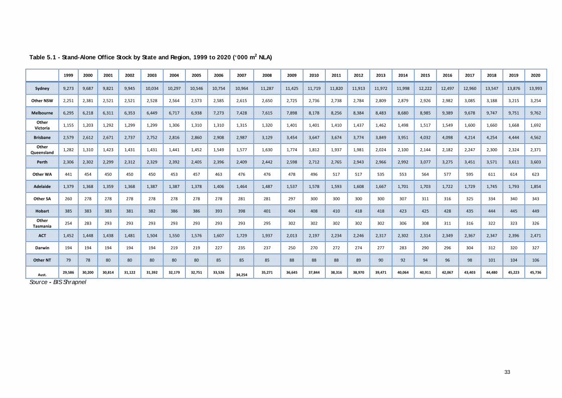
33

Table 5.1 - Stand-Alone Office Stock by State and Region, 1999 to 2020 (‘000 m2 NLA)

1999 2000 2001 2002 2003 2004 2005 2006 2007 2008 2009 2010 2011 2012 2013 2014 2015 2016 2017 2018 2019 2020

Sydney 9,273 9,687 9,821 9,945 10,034 10,297 10,546 10,754 10,964 11,287 11,425 11,719 11,820 11,913 11,972 11,998 12,222 12,497 12,960 13,547 13,876 13,993

Other NSW 2,251 2,381 2,521 2,521 2,528 2,564 2,573 2,585 2,615 2,650 2,725 2,736 2,738 2,784 2,809 2,879 2,926 2,982 3,085 3,188 3,215 3,254

Melbourne 6,295 6,218 6,311 6,353 6,449 6,717 6,938 7,273 7,428 7,615 7,898 8,178 8,256 8,384 8,483 8,680 8,985 9,389 9,678 9,747 9,751 9,762

Other Victoria 1,155 1,203 1,292 1,299 1,299 1,306 1,310 1,310 1,315 1,320 1,401 1,401 1,410 1,437 1,462 1,498 1,517 1,549 1,600 1,660 1,668 1,692

Brisbane 2,579 2,612 2,671 2,737 2,752 2,816 2,860 2,908 2,987 3,129 3,454 3,647 3,674 3,774 3,849 3,951 4,032 4,098 4,214 4,254 4,444 4,562

Other Queensland 1,282 1,310 1,423 1,431 1,431 1,441 1,452 1,549 1,577 1,630 1,774 1,812 1,937 1,981 2,024 2,100 2,144 2,182 2,247 2,300 2,324 2,371

Perth 2,306 2,302 2,299 2,312 2,329 2,392 2,405 2,396 2,409 2,442 2,598 2,712 2,765 2,943 2,966 2,992 3,077 3,275 3,451 3,571 3,611 3,603

Other WA 441 454 450 450 450 453 457 463 476 476 478 496 517 517 535 553 564 577 595 611 614 623

Adelaide 1,379 1,368 1,359 1,368 1,387 1,387 1,378 1,406 1,464 1,487 1,537 1,578 1,593 1,608 1,667 1,701 1,703 1,722 1,729 1,745 1,793 1,854

Other SA 260 278 278 278 278 278 278 278 281 281 297 300 300 300 300 307 311 316 325 334 340 343

Hobart 385 383 383 381 382 386 386 393 398 401 404 408 410 418 418 423 425 428 435 444 445 449

Other Tasmania 254 283 293 293 293 293 293 293 293 295 302 302 302 302 302 306 308 311 316 322 323 326

ACT 1,452 1,448 1,438 1,481 1,504 1,550 1,576 1,607 1,729 1,937 2,013 2,197 2,234 2,246 2,317 2,302 2,314 2,349 2,367 2,347 2,396 2,471

Darwin 194 194 194 194 194 219 219 227 235 237 250 270 272 274 277 283 290 296 304 312 320 327

Other NT 79 78 80 80 80 80 80 85 85 85 88 88 88 89 90 92 94 96 98 101 104 106

Aust. 29,586 30,200 30,814 31,122 31,392 32,179 32,751 33,526

34,254 35,271 36,645 37,844 38,316 38,970 39,471 40,064 40,911 42,067 43,403 44,480 45,223 45,736

Source - BIS Shrapnel

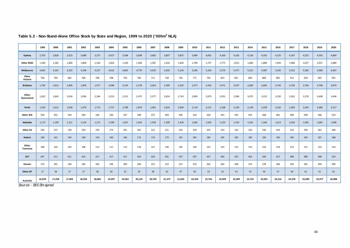
34

Table 5.2 - Non-Stand-Alone Office Stock by State and Region, 1999 to 2020 (‘000m2 NLA)

1999 2000 2001 2002 2003 2004 2005 2006 2007 2008 2009 2010 2011 2012 2013 2014 2015 2016 2017 2018 2019 2020

Sydney 2,703 2,828 2,923 3,080 3,275 3,427 3,508 3,608 3,682 3,807 3,875 3,984 4,062 4,100 4,165 4,136 4,102 4,155 4,187 4,253 4,593 4,864

Other NSW 1,583 1,582 1,860 1,860 1,540 1,856 1,540 1,560 1,587 1,634 1,664 1,709 1,747 1,775 1,815 1,846 1,889 1,944 1,986 2,027 2,057 2,080

Melbourne 4,065 4,161 4,255 4,338 4,527 4,632 4,665 4,779 4,925 5,050 5,140 5,290 5,336 5,379 5,477 5,551 5,487 5,342 5,322 5,585 5,989 6,407

Other Victoria 758 769 682 708 708 708 704 709 711 758 763 771 794 814 831 846 869 895 912 929 945 955

Brisbane 1,792 1,812 1,856 1,905 1,977 2,048 2,134 2,178 2,263 2,309 2,353 2,377 2,424 2,471 2,547 2,609 2,685 2,750 2,726 2,760 2,748 2,874

Other Queensland 1,832 1,842 2,034 2,096 2,184 2,253 2,351 2,475 2,577 2,654 2,743 2,809 2,873 2,931 2,996 3,075 3,152 3,230 3,301 3,370 3,408 3,446

Perth 1,593 1,612 1,630 1,674 1,713 1,757 1,798 1,874 1,961 2,024 2,069 2,118 2,131 2,108 2,169 2,199 2,258 2,326 2,383 2,443 2,480 2,517

Other WA 350 352 344 330 330 330 337 348 372 404 405 416 430 443 445 454 468 481 490 500 506 510

Adelaide 1,173 1,199 1,211 1,234 1,273 1,298 1,307 1,343 1,359 1,399 1,434 1,482 1,505 1,533 1,534 1,545 1,566 1,613 1,650 1,695 1,685 1,698

Other SA 240 237 239 250 259 274 291 302 315 321 326 329 333 333 333 333 336 344 352 359 363 368

Hobart 140 141 143 148 154 160 166 172 176 179 181 185 185 185 185 185 185 185 185 185 187 188

Other Tasmania 108 103 102 108 112 111 115 118 127 136 145 149 155 155 155 155 154 154 153 151 153 154

ACT 407 411 411 416 417 417 417 424 434 431 437 437 437 404 425 463 439 457 480 480 498 559

Darwin 179 181 184 184 185 196 200 206 221 222 237 252 262 264 268 272 278 284 292 301 304 309

Other NT 17 28 27 27 28 30 32 33 38 42 47 50 53 53 54 55 56 57 59 61 61 62

Australia 16,939 17,258 17,903 18,358 18,684 19,497 19,564 20,129 20,749 21,373 21,820 22,359 22,726 22,949 23,399 23,725 23,925 24,216 24,478 25,099 25,977 26,988

Source - BIS Shrapnel

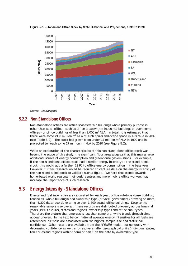
35

Figure 5.1 - Standalone Office Stock by State Historical and Projections, 1999 to 2020

. Source - BIS Shrapnel

5.2.2 Non Standalone Offices Non-standalone offices are office spaces within buildings whole primary purpose is other than as an office – such as office areas within industrial buildings or even home offices – or office buildings of less than 1,000 m2 NLA. In total, it is estimated that there were some 21.8 million m2 NLA of such non-stand-office space in Australia in 2009 (see Table 5.2). The stock has grown from under 17 million m2 NLA in 1999 and is projected to reach some 27 million m2 NLA by 2020 (see Figure 5.2). While an exploration of the characteristics of this non-stand-alone office stock was beyond the scope of this study, the significant floor area suggests that this may a large additional source of energy consumption and greenhouse gas emissions. For example, if the non-standalone office space had a similar energy intensity to the stand-alone stock, this would add a further 21 PJ to office energy consumption in the base year. However, further research would be required to capture data on the energy intensity of the non-stand-alone stock to validate such a figure. We note that trends towards home-based work, regional ‘hot-desk’ centres and more mobile office workers may increase the importance of such research.

5.3 Energy Intensity - Standalone Offices Energy and fuel intensities are calculated for each year, office sub-type (base building, tenancies, whole buildings) and ownership type (private, government) drawing on more than 4,300 data records relating to over 1,700 actual office buildings. Despite the reasonable sample size overall, these records are distributed unevenly across financial years (1999 to 2012), states and regions, ownership types and office sub- types. Therefore the picture that emerges is less than complete, while trends through time appear uneven. In the text below, national average energy intensities for all fuels are referenced, as these are associated with the highest sample size and statistical confidence. Other results are available from the NRBuild model, but generally with decreasing confidence as we try to resolve smaller geographical units (individual states, territories and regions within them) or partition the data by ownership type.

0

5000

10000

15000

20000

25000

30000

35000

40000

45000

50000

1999

2001

2003

2005

2007

2009

2011

2013

2015

2017

2019

('000

's N

LA)

Year

NT

ACT

Tasmania

SA

WA

Queensland

Victoria

NSW

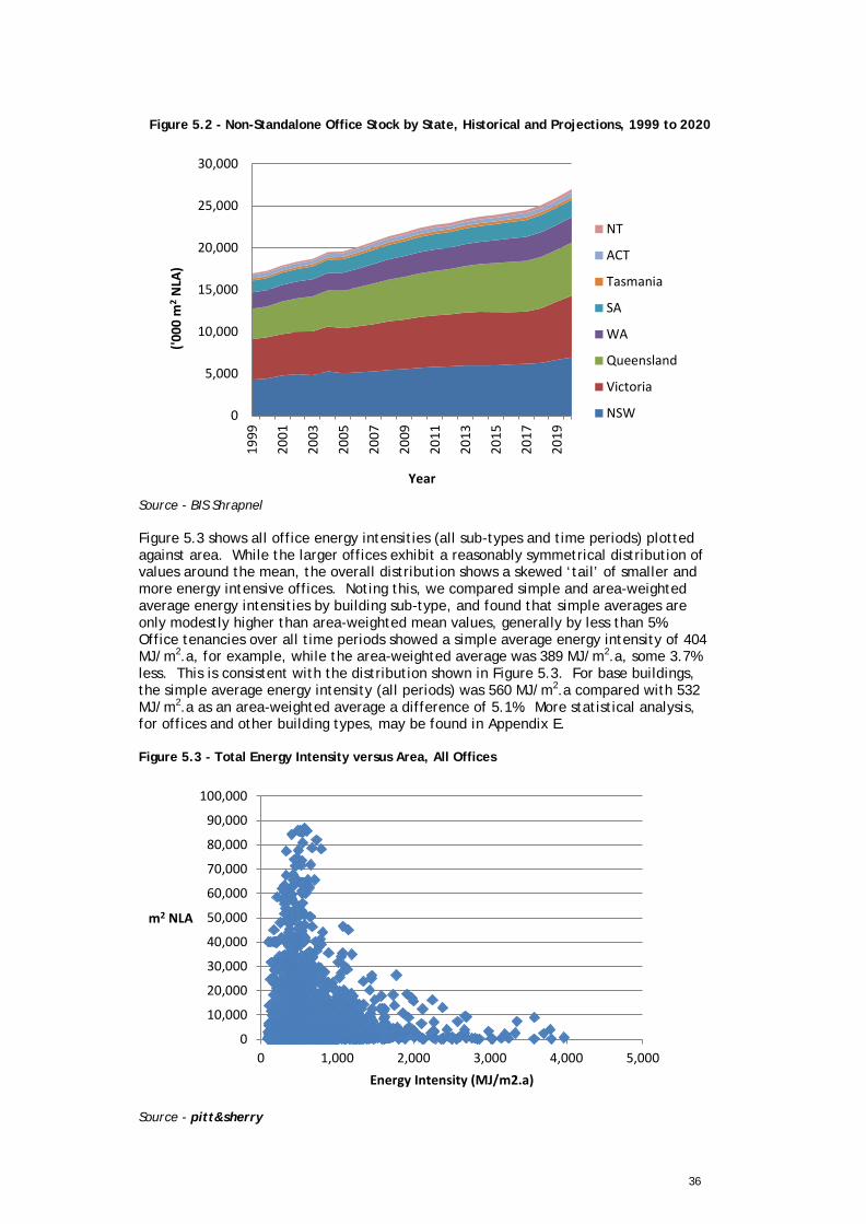
36

Figure 5.2 - Non-Standalone Office Stock by State, Historical and Projections, 1999 to 2020

. Source - BIS Shrapnel Figure 5.3 shows all office energy intensities (all sub-types and time periods) plotted against area. While the larger offices exhibit a reasonably symmetrical distribution of values around the mean, the overall distribution shows a skewed ‘tail’ of smaller and more energy intensive offices. Noting this, we compared simple and area-weighted average energy intensities by building sub-type, and found that simple averages are only modestly higher than area-weighted mean values, generally by less than 5%. Office tenancies over all time periods showed a simple average energy intensity of 404 MJ/m2.a, for example, while the area-weighted average was 389 MJ/m2.a, some 3.7% less. This is consistent with the distribution shown in Figure 5.3. For base buildings, the simple average energy intensity (all periods) was 560 MJ/m2.a compared with 532 MJ/m2.a as an area-weighted average a difference of 5.1%. More statistical analysis, for offices and other building types, may be found in Appendix E. Figure 5.3 - Total Energy Intensity versus Area, All Offices

. Source - pitt&sherry

0

5,000

10,000

15,000

20,000

25,000

30,000

1999

2001

2003

2005

2007

2009

2011

2013

2015

2017

2019

('000

m2 N

LA)

Year

NT

ACT

Tasmania

SA

WA

Queensland

Victoria

NSW

0

10,000

20,000

30,000

40,000

50,000

60,000

70,000

80,000

90,000

100,000

0 1,000 2,000 3,000 4,000 5,000

m2 NLA

Energy Intensity (MJ/m2.a)

37

For a more detailed examination of energy intensities, the data is broken down by office sub-type, state and region, ownership type and financial year.

5.3.1 Office Tenancies Figure 5.4 below shows the average annual energy intensity for office tenancies for the years 2001-2011, including linear regressions for the period back to 1999 and forward to 2020. In the base year of 2009, the average energy intensity of office tenancies in Australia is indicated to be around 385 MJ/m2.a. The results shown are based on area-weighted average energy intensities for all regions in Australia, for each year in which the sample size (n) was at least 95. On this basis, a trend was available for the years 2001 to 2011 informed by a total sample of 1,885 records totalling over 4 million m2 of office tenancies in Australia (all periods). Despite this, it can be seen that the values for average annual energy intensity vary considerably around the trend, although not by more than 50 MJ/m2.a in any year. This results in a very low R2 value of 0.04, indicating a very weak trend. 28 Further data capture would be required to establish trends with greater confidence. Despite this, we draw a weak conclusion that, on average, the energy intensity of office tenancies in Australia appears to have fallen modestly over the decade to 2011. The NRBuild model assumes this weak downward trend continues through to 2020, as it is reinforced by policy settings such as the Building Code of Australia and the Building Energy Efficiency Disclosure Act. Given the low confidence associated with national average energy intensity trends for office tenancies, the model does not rely upon finer ‘resolution’ results (for example comparing time series trends by ownership type, state or region), as progressively smaller sample sizes are available to support such results. However, sections 5.6 and 5.7 below report some results from the office tenancy analysis that differentiate average energy intensities by region or ownership type, where those results are supported by a sample size of at least 50 data records. Note that the user of the NRBuild model may specify their own ‘minimum n value’ and examine the results.

Figure 5.4 - Average Energy Intensity, Office Tenancies, Australia

....... Source - pitt&sherry

28 ‘R squared’ values vary between 0 and 1, with 1 indicating a perfect fit of data points to the trendline (all points appear exactly on the line). Progressively lower values indicate a poorer ‘fit’ of the data points to the trend and, as a result, lower confidence in the trendline itself.

R² = 0.0379

050

100150200250300350400450

1999

2001

2003

2005

2007

2009

2011

2013

2015

2017

2019

MJ/

m2 .a

Year

n>=95

Total n, all periods: 1885

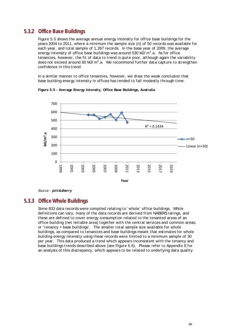
38

5.3.2 Office Base Buildings Figure 5.5 shows the average annual energy intensity for office base buildings for the years 2004 to 2011, where a minimum the sample size (n) of 50 records was available for each year, and total sample of 1,267 records. In the base year of 2009, the average energy intensity of office base buildings was around 530 MJ/m2.a. As for office tenancies, however, the fit of data to trend is quite poor, although again the variability does not exceed around 60 MJ/m2.a. We recommend further data capture to strengthen confidence in this trend. In a similar manner to office tenancies, however, we draw the weak conclusion that base building energy intensity in offices has tended to fall modestly through time. Figure 5.5 - Average Energy Intensity, Office Base Buildings, Australia

Source - pitt&sherry

5.3.3 Office Whole Buildings Some 833 data records were compiled relating to ‘whole’ office buildings. While definitions can vary, many of the data records are derived from NABERS ratings, and these are defined to cover energy consumption related to the tenanted areas of an office building (net lettable area) together with the central services and common areas, or ‘tenancy + base buildings’. The smaller total sample size available for whole buildings, as compared to tenancies and base buildings meant that estimates for whole building energy intensity using these records were limited to a minimum sample of 30 per year. This data produced a trend which appears inconsistent with the tenancy and base buildings trends described above (see Figure 5.6). Please refer to Appendix E for an analysis of this discrepancy, which appears to be related to underlying data quality.

R² = 0.1434

0

100

200

300

400

500

600

700

1999

2001

2003

2005

2007

2009

2011

2013

2015

2017

2019

MJ/

m2 .a

Year

n>50

Linear (n>50)

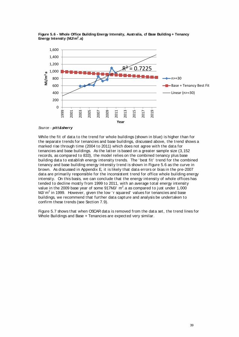
39

Figure 5.6 - Whole Office Building Energy Intensity, Australia, cf Base Building + Tenancy Energy Intensity (MJ/m2.a)

Source - pitt&sherry While the fit of data to the trend for whole buildings (shown in blue) is higher than for the separate trends for tenancies and base buildings, discussed above, the trend shows a marked rise through time (2004 to 2011) which does not agree with the data for tenancies and base buildings. As the latter is based on a greater sample size (3,152 records, as compared to 833), the model relies on the combined tenancy plus base building data to establish energy intensity trends. The ‘best fit’ trend for the combined tenancy and base building energy intensity trend is shown in Figure 5.6 as the curve in brown. As discussed in Appendix E, it is likely that data errors or bias in the pre-2007 data are primarily responsible for the inconsistent trend for office whole building energy intensity. On this basis, we can conclude that the energy intensity of whole offices has tended to decline mostly from 1999 to 2011, with an average total energy intensity value in the 2009 base year of some 917MJ/ m2.a as compared to just under 1,000 MJ/m2 in 1999. However, given the low ‘r squared’ values for tenancies and base buildings, we recommend that further data capture and analysis be undertaken to confirm these trends (see Section 7.9). Figure 5.7 shows that when OSCAR data is removed from the data set, the trend lines for Whole Buildings and Base + Tenancies are expected very similar.

R² = 0.7225

0

200

400

600

800

1,000

1,200

1,400

1,600

1999

2001

2003

2005

2007

2009

2011

2013

2015

2017

2019

MJ/

m2.

a

Year

n>=30

Base + Tenancy Best Fit

Linear (n>=30)

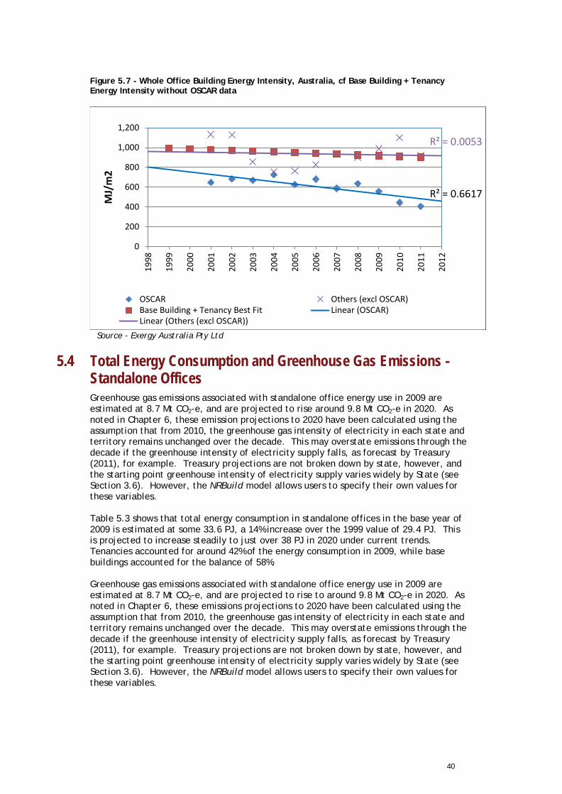
40

Figure 5.7 - Whole Office Building Energy Intensity, Australia, cf Base Building + Tenancy Energy Intensity without OSCAR data

..Source - Exergy Australia Pty Ltd

5.4 Total Energy Consumption and Greenhouse Gas Emissions - Standalone Offices Greenhouse gas emissions associated with standalone office energy use in 2009 are estimated at 8.7 Mt CO2-e, and are projected to rise around 9.8 Mt CO2-e in 2020. As noted in Chapter 6, these emission projections to 2020 have been calculated using the assumption that from 2010, the greenhouse gas intensity of electricity in each state and territory remains unchanged over the decade. This may overstate emissions through the decade if the greenhouse intensity of electricity supply falls, as forecast by Treasury (2011), for example. Treasury projections are not broken down by state, however, and the starting point greenhouse intensity of electricity supply varies widely by State (see Section 3.6). However, the NRBuild model allows users to specify their own values for these variables. Table 5.3 shows that total energy consumption in standalone offices in the base year of 2009 is estimated at some 33.6 PJ, a 14% increase over the 1999 value of 29.4 PJ. This is projected to increase steadily to just over 38 PJ in 2020 under current trends. Tenancies accounted for around 42% of the energy consumption in 2009, while base buildings accounted for the balance of 58%. Greenhouse gas emissions associated with standalone office energy use in 2009 are estimated at 8.7 Mt CO2-e, and are projected to rise to around 9.8 Mt CO2-e in 2020. As noted in Chapter 6, these emissions projections to 2020 have been calculated using the assumption that from 2010, the greenhouse gas intensity of electricity in each state and territory remains unchanged over the decade. This may overstate emissions through the decade if the greenhouse intensity of electricity supply falls, as forecast by Treasury (2011), for example. Treasury projections are not broken down by state, however, and the starting point greenhouse intensity of electricity supply varies widely by State (see Section 3.6). However, the NRBuild model allows users to specify their own values for these variables.

R² = 0.6617

R² = 0.0053

0

200

400

600

800

1,000

1,200

1998

1999

2000

2001

2002

2003

2004

2005

2006

2007

2008

2009

2010

2011

2012

MJ/

m2

OSCAR Others (excl OSCAR)Base Building + Tenancy Best Fit Linear (OSCAR)Linear (Others (excl OSCAR))

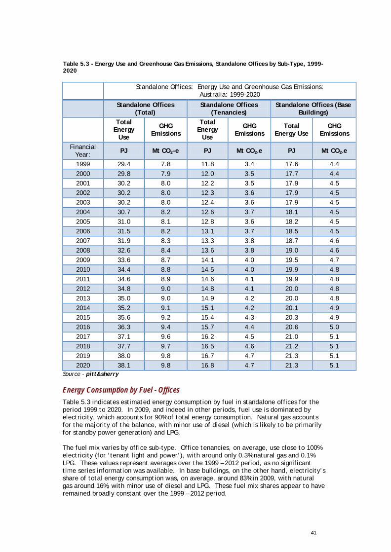
41

Table 5.3 - Energy Use and Greenhouse Gas Emissions, Standalone Offices by Sub-Type, 1999-2020

Standalone Offices: Energy Use and Greenhouse Gas Emissions:

Australia: 1999-2020

Standalone Offices

(Total) Standalone Offices

(Tenancies) Standalone Offices (Base

Buildings)

Total Energy

Use

GHG Emissions

Total Energy

Use

GHG Emissions

Total Energy Use

GHG Emissions

Financial Year: PJ Mt CO2-e PJ Mt CO2-e PJ Mt CO2-e

1999 29.4 7.8 11.8 3.4 17.6 4.4 2000 29.8 7.9 12.0 3.5 17.7 4.4 2001 30.2 8.0 12.2 3.5 17.9 4.5 2002 30.2 8.0 12.3 3.6 17.9 4.5 2003 30.2 8.0 12.4 3.6 17.9 4.5 2004 30.7 8.2 12.6 3.7 18.1 4.5 2005 31.0 8.1 12.8 3.6 18.2 4.5 2006 31.5 8.2 13.1 3.7 18.5 4.5 2007 31.9 8.3 13.3 3.8 18.7 4.6 2008 32.6 8.4 13.6 3.8 19.0 4.6 2009 33.6 8.7 14.1 4.0 19.5 4.7 2010 34.4 8.8 14.5 4.0 19.9 4.8 2011 34.6 8.9 14.6 4.1 19.9 4.8 2012 34.8 9.0 14.8 4.1 20.0 4.8 2013 35.0 9.0 14.9 4.2 20.0 4.8 2014 35.2 9.1 15.1 4.2 20.1 4.9 2015 35.6 9.2 15.4 4.3 20.3 4.9 2016 36.3 9.4 15.7 4.4 20.6 5.0 2017 37.1 9.6 16.2 4.5 21.0 5.1 2018 37.7 9.7 16.5 4.6 21.2 5.1 2019 38.0 9.8 16.7 4.7 21.3 5.1 2020 38.1 9.8 16.8 4.7 21.3 5.1

Source - pitt&sherry

Energy Consumption by Fuel - Offices Table 5.3 indicates estimated energy consumption by fuel in standalone offices for the period 1999 to 2020. In 2009, and indeed in other periods, fuel use is dominated by electricity, which accounts for 90% of total energy consumption. Natural gas accounts for the majority of the balance, with minor use of diesel (which is likely to be primarily for standby power generation) and LPG. The fuel mix varies by office sub-type. Office tenancies, on average, use close to 100% electricity (for ‘tenant light and power’), with around only 0.3% natural gas and 0.1% LPG. These values represent averages over the 1999 – 2012 period, as no significant time series information was available. In base buildings, on the other hand, electricity’s share of total energy consumption was, on average, around 83% in 2009, with natural gas around 16%, with minor use of diesel and LPG. These fuel mix shares appear to have remained broadly constant over the 1999 – 2012 period.

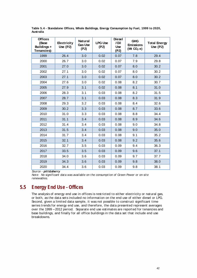
42

Table 5.4 - Standalone Offices, Whole Buildings, Energy Consumption by Fuel, 1999 to 2020, Australia

Offices (Base

Buildings + Tenancies):

Electricity Use (PJ)

Natural Gas Use

(PJ)

LPG Use (PJ)

Diesel/Oil Use (PJ)

GHG Emissions (Mt CO2-e)

Total Energy Use (PJ)

1999 26.4 3.0 0.02 0.07 7.8 29.4

2000 26.7 3.0 0.02 0.07 7.9 29.8

2001 27.0 3.0 0.02 0.07 8.0 30.2

2002 27.1 3.0 0.02 0.07 8.0 30.2

2003 27.1 3.0 0.02 0.07 8.0 30.2

2004 27.6 3.0 0.02 0.08 8.2 30.7

2005 27.9 3.1 0.02 0.08 8.1 31.0

2006 28.3 3.1 0.03 0.08 8.2 31.5

2007 28.7 3.1 0.03 0.08 8.3 31.9

2008 29.3 3.2 0.03 0.08 8.4 32.6

2009 30.2 3.3 0.03 0.08 8.7 33.6

2010 31.0 3.3 0.03 0.08 8.8 34.4

2011 31.1 3.4 0.03 0.08 8.9 34.6

2012 31.4 3.4 0.03 0.08 9.0 34.8

2013 31.5 3.4 0.03 0.08 9.0 35.0

2014 31.7 3.4 0.03 0.08 9.1 35.2

2015 32.1 3.4 0.03 0.08 9.2 35.6

2016 32.7 3.5 0.03 0.09 9.4 36.3

2017 33.5 3.5 0.03 0.09 9.6 37.1

2018 34.0 3.6 0.03 0.09 9.7 37.7

2019 34.3 3.6 0.03 0.09 9.8 38.0

2020 34.4 3.6 0.03 0.09 9.8 38.1 Source - pitt&sherry Note: No significant data was available on the consumption of Green Power or on-site renewables.

5.5 Energy End Use - Offices The analysis of energy end use in offices is restricted to either electricity or natural gas, or both, as the data sets included no information on the end use of either diesel or LPG. Second, given a limited data sample, it was not possible to construct significant time series trends for energy end use, and therefore, the data presented represent averages over the 1999 – 2012 period. Separate end use estimates are reported for tenancies and base buildings, and finally for all office buildings in the data set that include end use breakdowns.

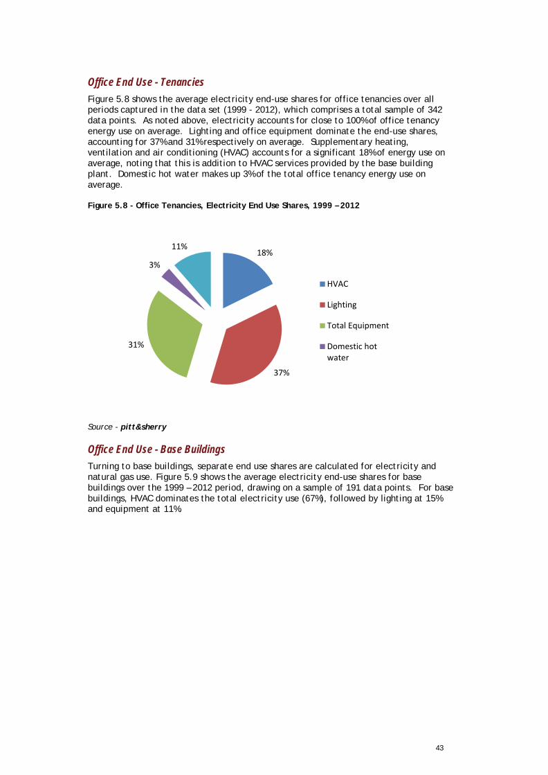
43

Office End Use - Tenancies Figure 5.8 shows the average electricity end-use shares for office tenancies over all periods captured in the data set (1999 - 2012), which comprises a total sample of 342 data points. As noted above, electricity accounts for close to 100% of office tenancy energy use on average. Lighting and office equipment dominate the end-use shares, accounting for 37% and 31% respectively on average. Supplementary heating, ventilation and air conditioning (HVAC) accounts for a significant 18% of energy use on average, noting that this is addition to HVAC services provided by the base building plant. Domestic hot water makes up 3% of the total office tenancy energy use on average.

Figure 5.8 - Office Tenancies, Electricity End Use Shares, 1999 – 2012 .

. Source - pitt&sherry

Office End Use - Base Buildings Turning to base buildings, separate end use shares are calculated for electricity and natural gas use. Figure 5.9 shows the average electricity end-use shares for base buildings over the 1999 – 2012 period, drawing on a sample of 191 data points. For base buildings, HVAC dominates the total electricity use (67%), followed by lighting at 15% and equipment at 11%.

18%

37%

31%

3%

11%

HVAC

Lighting

Total Equipment

Domestic hotwater

44

Figure 5.9 - Office Base Buildings, Electricity End Use Shares, 1999 – 2012

. Source - pitt&sherry With respect to natural gas, a smaller sample of 62 end use data points indicate that space heating is the dominant end use of natural gas in office base buildings, with an average end use share of almost half of gas use (49%), as shown in Figure 5.10. Domestic hot water accounts for around 8% of gas use, while a significant residual of ‘other gas use’ is not attributed to particular end uses in the data available to this study. Figure 5.10 - Office Base Buildings, Natural Gas End Use Shares, 1999 - 2012

. Source - pitt&sherry

67%

15%

11%

2% 4%

HVAC

Lighting

Total Equipment

Domestic hot water

Other electricalprocess

49%

8% 4%

39% Space Heating

Domestic Hot Water

Kitchen/ catering

Other gas use

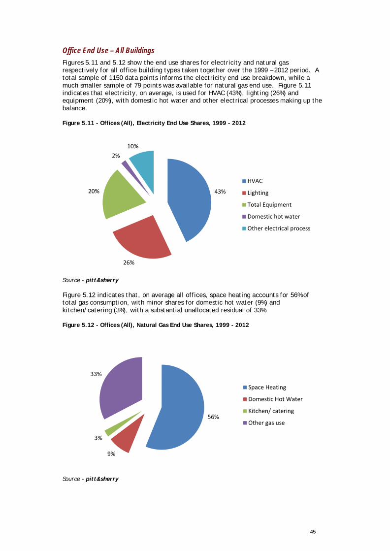
45

Office End Use – All Buildings Figures 5.11 and 5.12 show the end use shares for electricity and natural gas respectively for all office building types taken together over the 1999 – 2012 period. A total sample of 1150 data points informs the electricity end use breakdown, while a much smaller sample of 79 points was available for natural gas end use. Figure 5.11 indicates that electricity, on average, is used for HVAC (43%), lighting (26%) and equipment (20%), with domestic hot water and other electrical processes making up the balance. Figure 5.11 - Offices (All), Electricity End Use Shares, 1999 - 2012

. Source - pitt&sherry Figure 5.12 indicates that, on average all offices, space heating accounts for 56% of total gas consumption, with minor shares for domestic hot water (9%) and kitchen/catering (3%), with a substantial unallocated residual of 33%. Figure 5.12 - Offices (All), Natural Gas End Use Shares, 1999 - 2012

. Source - pitt&sherry

43%

26%

20%

2% 10%

HVAC

Lighting

Total Equipment

Domestic hot water

Other electrical process

56%

9%

3%

33%

Space Heating

Domestic Hot Water

Kitchen/ catering

Other gas use

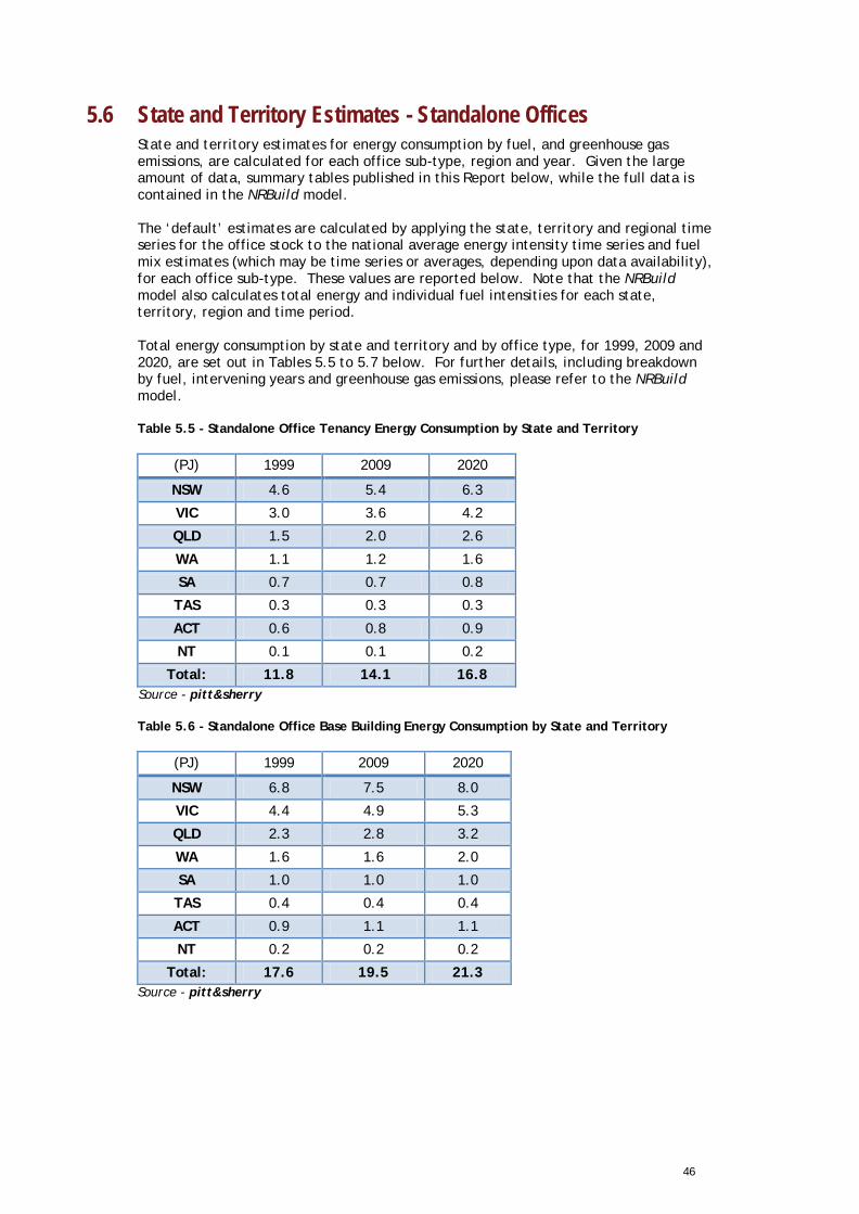
46

5.6 State and Territory Estimates - Standalone Offices State and territory estimates for energy consumption by fuel, and greenhouse gas emissions, are calculated for each office sub-type, region and year. Given the large amount of data, summary tables published in this Report below, while the full data is contained in the NRBuild model. The ‘default’ estimates are calculated by applying the state, territory and regional time series for the office stock to the national average energy intensity time series and fuel mix estimates (which may be time series or averages, depending upon data availability), for each office sub-type. These values are reported below. Note that the NRBuild model also calculates total energy and individual fuel intensities for each state, territory, region and time period. Total energy consumption by state and territory and by office type, for 1999, 2009 and 2020, are set out in Tables 5.5 to 5.7 below. For further details, including breakdown by fuel, intervening years and greenhouse gas emissions, please refer to the NRBuild model. Table 5.5 - Standalone Office Tenancy Energy Consumption by State and Territory

(PJ) 1999 2009 2020

NSW 4.6 5.4 6.3

VIC 3.0 3.6 4.2

QLD 1.5 2.0 2.6

WA 1.1 1.2 1.6

SA 0.7 0.7 0.8

TAS 0.3 0.3 0.3

ACT 0.6 0.8 0.9

NT 0.1 0.1 0.2

Total: 11.8 14.1 16.8 Source - pitt&sherry Table 5.6 - Standalone Office Base Building Energy Consumption by State and Territory

(PJ) 1999 2009 2020

NSW 6.8 7.5 8.0

VIC 4.4 4.9 5.3

QLD 2.3 2.8 3.2

WA 1.6 1.6 2.0

SA 1.0 1.0 1.0

TAS 0.4 0.4 0.4

ACT 0.9 1.1 1.1

NT 0.2 0.2 0.2

Total: 17.6 19.5 21.3 Source - pitt&sherry

47

Table 5.7 - Standalone Office Whole Buildings Energy Consumption by State and Territory

(PJ) 1999 2009 2020

NSW 11.5 13.0 14.4

VIC 7.4 8.5 9.5

QLD 3.8 4.8 5.8

WA 2.7 2.8 3.5

SA 1.6 1.7 1.8

TAS 0.6 0.6 0.6

ACT 1.4 1.8 2.1

NT 0.3 0.3 0.4

Total: 29.4 33.6 38.1 Source - pitt&sherry

5.6.1 State, Territory and Regional Energy Intensity Calculation - Offices It was noted above that the NRBuild model also calculates total energy and individual fuel intensities for each state, territory, region and time period, subject to data availability. However, the overall sample size (for all the data sets) is generally too small to allow meaningful regression analyses for the evolution of energy intensity (or fuel mix) at the level of each state, territory or region. Indeed, for some combinations of building type and state/territory/region, there are no data records at all. However, where sufficient data is available, we report energy intensities by state/territory, as an average over the 1999 – 2012 time period, along with the underlying sample size. These may provide useful comparisons, but care should be exercised in their interpretation due to limited statistical significance. These results are summarised in Tables 5.8 to 5.10 below for privately owned offices. Data for government-owned offices is shown in Section 5.7 below. Where no values are shown, this indicates that either no data was available for that state, territory or region, or otherwise the data sample that fell below the minimum noted. Note that the NRBuild model allows the user to test their preferred values for energy intensity over time (after the base year of 2009). Values relevant to a particular state, territory or region could inserted in the model, for any building type or sub-type, and the modelled total energy and greenhouse calculations would be valid for that state, territory or region only. Modelled outputs for other states/regions would not, however, be valid. Note also that, with respect to the tables below, the model user may specify their own minimum ‘n’ values, as alternatives to those shown.

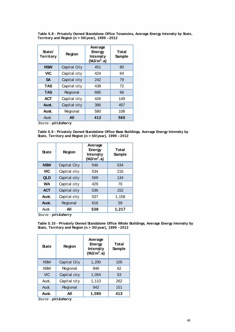
48

Table 5.8 - Privately Owned Standalone Office Tenancies, Average Energy Intensity by State, Territory and Region (n > 50/year), 1999 – 2012

State/ Territory Region

Average Energy

Intensity (MJ/m2.a)

Total Sample

NSW Capital City 451 80

VIC Capital city 424 64

SA Capital city 242 79

TAS Capital city 438 72

TAS Regional 685 66

ACT Capital city 426 149

Aust. Capital city 386 457

Aust. Regional 580 108

Aust. All 412 565 Source - pitt&sherry Table 5.9 - Privately Owned Standalone Office Base Buildings, Average Energy Intensity by State, Territory and Region (n > 50/year), 1999 – 2012

State Region

Average Energy

Intensity (MJ/m2.a)

Total Sample

NSW Capital City 546 534

VIC Capital city 534 216

QLD Capital city 569 134

WA Capital city 429 70

ACT Capital city 536 152

Aust. Capital city 537 1,158

Aust. Regional 616 59

Aust. All 538 1,217 Source - pitt&sherry Table 5.10 - Privately Owned Standalone Office Whole Buildings, Average Energy Intensity by State, Territory and Region (n > 30/year), 1999 – 2012

State Region

Average Energy

Intensity (MJ/m2.a)

Total Sample

NSW Capital City 1,290 105

NSW Regional 846 62

VIC Capital city 1,054 53

Aust. Capital city 1,113 262

Aust. Regional 942 151

Aust. All 1,085 413 Source - pitt&sherry

49

5.7 Government Owned Standalone Offices This section reports the modelled results for average energy intensities of the government-owned segment of the offices data set, by building type. As above, the data shown is an average of the 1999 to 2012 period due to insufficient time series information, and values are only shown where the sample size they are based on exceeds the minimum threshold specified. These results are then compared with the results for the privately-owned office stock, as reported above. Note that it was not possible to construct estimates of total energy consumption or greenhouse gas emissions within the government-owned portion of the stock, not because of insufficient data on average energy intensities, but rather due to a lack of the data on the physical extent of the government-owned office stock. This data does not appear to be reported in any consolidated format, and although BIS Shrapnel was able to estimate the stock for certain states and certain years, no overall stock model could be constructed. Also, we would expect the government-owned portion of the office stock to decline markedly since 1999, at least in some states and territories, due to extensive sale and lease-back initiatives by all governments. We note, in Section 6.9 below, the uncertainty about the extent of the government-owned office stock is one data hurdle that should be able to be cleared with further collaboration between the Commonwealth and states and territories. Tables 5.11 and 5.12 below show the average energy intensities of the government-owned office buildings (tenancies and whole buildings respectively) in the data set, by state, territory and region, over the period 1999 – 2012, along with the sample sizes underpinning these observations. As above, where no values are shown, this indicates that either no data was available for that state, territory or region, or otherwise the data sample that fell below the minimum noted. Note that no significant data was available on the energy intensity of government owned office base buildings. Table 5.11 - Government Owned Standalone Office Tenancies, Average Energy Intensity by State, Territory and Region (n > 50/year), 1999 – 2012

State Region

Average Energy

Intensity (MJ/m2.a)

Total Sample

SA Capital city 374 668

SA Regional 310 200

ACT Capital city 392 84

NT Capital city 333 207

NT Regional 323 87

Aust. Capital city 381 988

Aust. Regional 329 332

Aust. All 377 1,320 Source - pitt&sherry

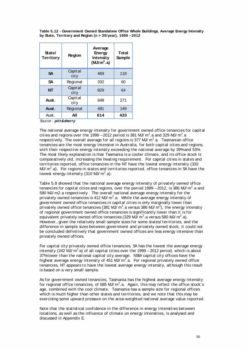
50

Table 5.12 - Government Owned Standalone Office Whole Buildings, Average Energy Intensity by State, Territory and Region (n > 30/year), 1999 – 2012

State/ Territory Region

Average Energy

Intensity (MJ/m2.a)

Total Sample

SA Capital city 469 118

SA Regional 332 60

NT Capital city 829 64

Aust. Capital city 648 271

Aust. Regional 481 149

Aust. All 614 420 Source - pitt&sherry The national average energy intensity for government owned office tenancies for capital cities and regions over the 1999 – 2012 period is 381 MJ/m2.a and 329 MJ/m2.a respectively. The overall average for all regions is 377 MJ/m2.a. Tasmanian office tenancies are the most energy intensive in Australia, for both capital cities and regions, with their respective energy intensity exceeding the national average by 39% and 53%. The most likely explanation is that Tasmania is a cooler climate, and its office stock is comparatively old, increasing the heating requirement. For capital cities in states and territories reported, office tenancies in the NT have the lowest energy intensity (333 MJ/m2.a). For regions in states and territories reported, office tenancies in SA have the lowest energy intensity (310 MJ/m2.a). Table 5.8 showed that the national average energy intensity of privately owned office tenancies for capital cities and regions, over the period 1999 – 2012, is 386 MJ/m2.a and 580 MJ/m2.a respectively. The overall national average energy intensity for the privately owned tenancies is 412 MJ/m2.a. While the average energy intensity of government owned office tenancies in capital cities is only marginally lower than privately owned office tenancies (381 MJ/m2.a versus 386 MJ/m2), the energy intensity of regional government owned office tenancies is significantly lower than it is for equivalent privately owned office tenancies (329 MJ/m2.a versus 580 MJ/m2.a). However, given the relatively small sample sizes for some states/territories, and the difference in sample sizes between government and privately owned stock, it could not be concluded definitively that government owned offices are less energy intensive than privately owned offices. For capital city privately owned office tenancies, SA has the lowest the average energy intensity (242 MJ/m2.a) of all capital cities over the 1999 – 2012 period, which is about 37% lower than the national capital city average. NSW capital city offices have the highest average energy intensity of 451 MJ/m2.a. For regional privately owned office tenancies, NT appears to have the lowest average energy intensity, although this result is based on a very small sample. As for government owned tenancies, Tasmania has the highest average energy intensity for regional office tenancies, of 685 MJ/m2.a. Again, this may reflect the office stock’s age, combined with the cool climate. Tasmania has a sample size for regional offices which is much higher than other states and territories, and we note that this may be exercising some upward pressure on the area-weighted national average value reported. Note that the statistical confidence in the difference in energy intensities between locations, as well as the influence of climate on energy intensities, is analysed and discussed in Appendix E.

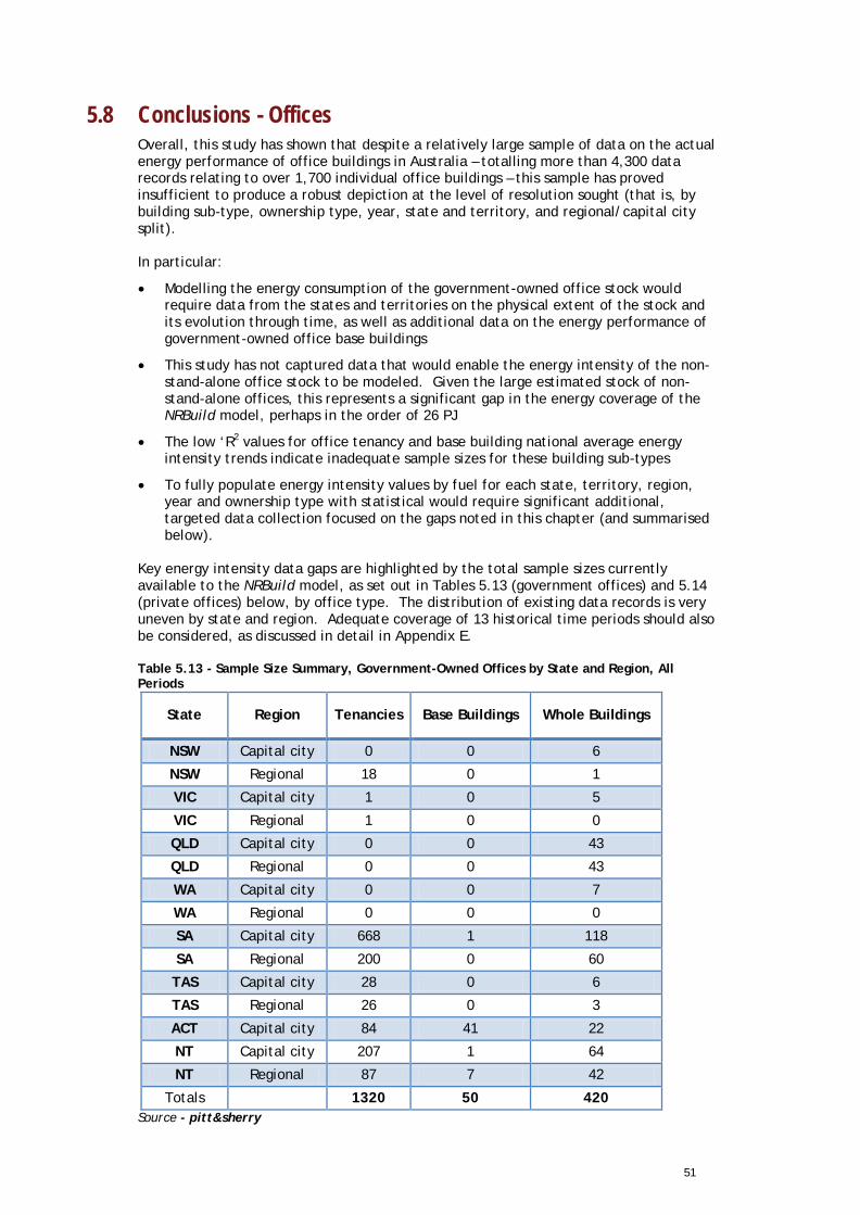
51

5.8 Conclusions - Offices Overall, this study has shown that despite a relatively large sample of data on the actual energy performance of office buildings in Australia – totalling more than 4,300 data records relating to over 1,700 individual office buildings – this sample has proved insufficient to produce a robust depiction at the level of resolution sought (that is, by building sub-type, ownership type, year, state and territory, and regional/capital city split). In particular:

• Modelling the energy consumption of the government-owned office stock would require data from the states and territories on the physical extent of the stock and its evolution through time, as well as additional data on the energy performance of government-owned office base buildings

• This study has not captured data that would enable the energy intensity of the non-stand-alone office stock to be modeled. Given the large estimated stock of non-stand-alone offices, this represents a significant gap in the energy coverage of the NRBuild model, perhaps in the order of 26 PJ

• The low ‘R2 values for office tenancy and base building national average energy intensity trends indicate inadequate sample sizes for these building sub-types

• To fully populate energy intensity values by fuel for each state, territory, region, year and ownership type with statistical would require significant additional, targeted data collection focused on the gaps noted in this chapter (and summarised below).

Key energy intensity data gaps are highlighted by the total sample sizes currently available to the NRBuild model, as set out in Tables 5.13 (government offices) and 5.14 (private offices) below, by office type. The distribution of existing data records is very uneven by state and region. Adequate coverage of 13 historical time periods should also be considered, as discussed in detail in Appendix E. Table 5.13 - Sample Size Summary, Government-Owned Offices by State and Region, All Periods

State Region Tenancies Base Buildings Whole Buildings

NSW Capital city 0 0 6

NSW Regional 18 0 1

VIC Capital city 1 0 5

VIC Regional 1 0 0

QLD Capital city 0 0 43

QLD Regional 0 0 43

WA Capital city 0 0 7

WA Regional 0 0 0

SA Capital city 668 1 118

SA Regional 200 0 60

TAS Capital city 28 0 6

TAS Regional 26 0 3

ACT Capital city 84 41 22

NT Capital city 207 1 64

NT Regional 87 7 42

Totals 1320 50 420 Source - pitt&sherry

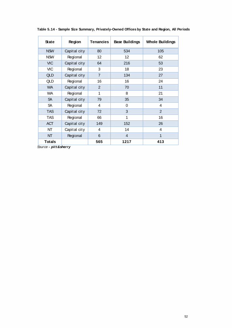
52

Table 5.14 - Sample Size Summary, Privately-Owned Offices by State and Region, All Periods

State Region Tenancies Base Buildings Whole Buildings

NSW Capital city 80 534 105

NSW Regional 12 12 62

VIC Capital city 64 216 53

VIC Regional 3 18 23

QLD Capital city 7 134 27

QLD Regional 16 16 24

WA Capital city 2 70 11

WA Regional 1 8 21

SA Capital city 79 35 34

SA Regional 4 0 4

TAS Capital city 72 3 2

TAS Regional 66 1 16

ACT Capital city 149 152 26

NT Capital city 4 14 4

NT Regional 6 4 1

Totals 565 1217 413 Source - pitt&sherry

53

6. Hotels 6.1 Introduction

This chapter presents key findings and underlying assumptions for hotels/motels, as modelled in NRBuild. The scope includes hotels and motels with at least 5 rooms but excludes serviced apartments. It also excludes hotels which are part of casinos, but where the hotel energy could not be separated from the casino building’s total energy. For the hotel/motel stock, in addition to there being a limited time series of energy data, the sample size of hotels with energy data was relatively small.

6.2 Stock Estimates - Hotels The stock of hotel/motel space in Australia has been estimated by BIS Shrapnel, drawing on a wide range of data sources and estimation techniques, as summarised in Chapter 4, with further detail in Appendix C. Hotel/motel floor space is calculated based on the number of hotel/motel rooms. The rooms data is sourced from the ABS (ABS Cat 8635.0), but the geographic segmentation is limited by the fact that several fields are not published at a detailed level for hotel star ratings because of confidentiality issues. The measure of accommodation floor space is intended not just to cover the actual rooms but all areas associated with servicing those rooms, including related office space, conference facilities, and dining facilities. The following ratios were applied to room numbers to estimate total floor space of hotels/motels:

• 1-2 star hotel/motel rooms, 35m2 per room

• 3 star hotel/motel rooms, 40m2 per room

• 4 star hotel/motel rooms, 70m2 per room

• 5 star hotel/motel, 85m2 per room.

In the base year of 2009, hotels/motels are estimated to have comprised some 10.7 million m2 net lettable area across Australia as a whole (see Table 6.1). Historically, the stock grew at an average rate of 1.1% per year between 1999 and 2011, and it is projected to continue to grow to 2020 at around 1.6% per year. New South Wales comprises the largest share of the hotel/motel stock by state, however, that share is expected to fall slightly from 38.6% to 37.7% over the 2009 to 2020 period. As for offices over the same period, the shares of Queensland and Western Australia are expected to increase, from 14.2% to 15.2% (QLD) and from 8.4% to 9.3% (WA).

6.3 Energy Intensity - Hotels Energy and fuel intensities are calculated for each year drawing on 208 data records relating to 195 actual hotels. The sample size is reasonably small, and records are distributed unevenly across financial years (1999 to 2012), and states and regions. For example, there are data records for the year 2000, but none between 2000 and 2005, while about 50% of the total data records are for the years 2010 and 2011.

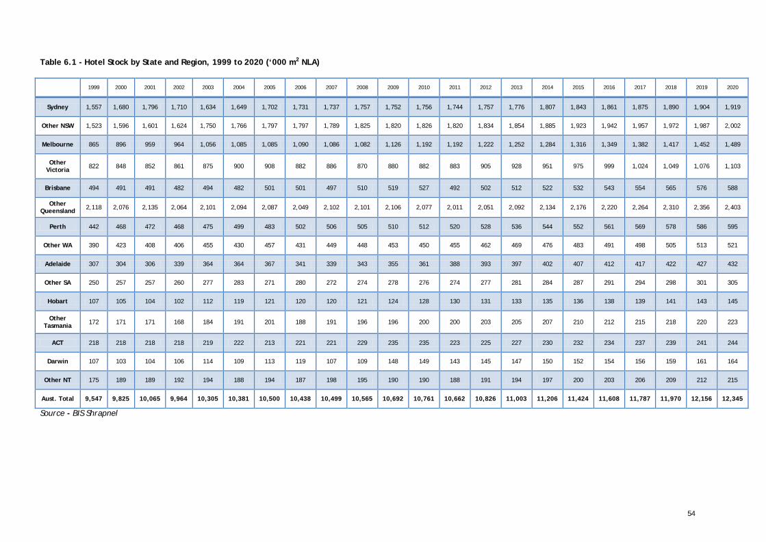
54

Table 6.1 - Hotel Stock by State and Region, 1999 to 2020 (‘000 m2 NLA)

1999 2000 2001 2002 2003 2004 2005 2006 2007 2008 2009 2010 2011 2012 2013 2014 2015 2016 2017 2018 2019 2020

Sydney 1,557 1,680 1,796 1,710 1,634 1,649 1,702 1,731 1,737 1,757 1,752 1,756 1,744 1,757 1,776 1,807 1,843 1,861 1,875 1,890 1,904 1,919

Other NSW 1,523 1,596 1,601 1,624 1,750 1,766 1,797 1,797 1,789 1,825 1,820 1,826 1,820 1,834 1,854 1,885 1,923 1,942 1,957 1,972 1,987 2,002

Melbourne 865 896 959 964 1,056 1,085 1,085 1,090 1,086 1,082 1,126 1,192 1,192 1,222 1,252 1,284 1,316 1,349 1,382 1,417 1,452 1,489

Other Victoria 822 848 852 861 875 900 908 882 886 870 880 882 883 905 928 951 975 999 1,024 1,049 1,076 1,103

Brisbane 494 491 491 482 494 482 501 501 497 510 519 527 492 502 512 522 532 543 554 565 576 588

Other Queensland 2,118 2,076 2,135 2,064 2,101 2,094 2,087 2,049 2,102 2,101 2,106 2,077 2,011 2,051 2,092 2,134 2,176 2,220 2,264 2,310 2,356 2,403

Perth 442 468 472 468 475 499 483 502 506 505 510 512 520 528 536 544 552 561 569 578 586 595

Other WA 390 423 408 406 455 430 457 431 449 448 453 450 455 462 469 476 483 491 498 505 513 521

Adelaide 307 304 306 339 364 364 367 341 339 343 355 361 388 393 397 402 407 412 417 422 427 432

Other SA 250 257 257 260 277 283 271 280 272 274 278 276 274 277 281 284 287 291 294 298 301 305

Hobart 107 105 104 102 112 119 121 120 120 121 124 128 130 131 133 135 136 138 139 141 143 145

Other Tasmania 172 171 171 168 184 191 201 188 191 196 196 200 200 203 205 207 210 212 215 218 220 223

ACT 218 218 218 218 219 222 213 221 221 229 235 235 223 225 227 230 232 234 237 239 241 244

Darwin 107 103 104 106 114 109 113 119 107 109 148 149 143 145 147 150 152 154 156 159 161 164

Other NT 175 189 189 192 194 188 194 187 198 195 190 190 188 191 194 197 200 203 206 209 212 215

Aust. Total 9,547 9,825 10,065 9,964 10,305 10,381 10,500 10,438 10,499 10,565 10,692 10,761 10,662 10,826 11,003 11,206 11,424 11,608 11,787 11,970 12,156 12,345

Source - BIS Shrapnel

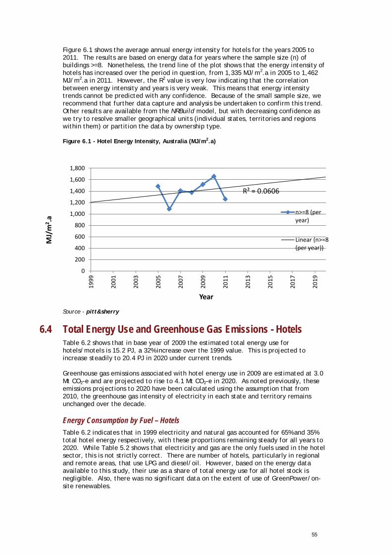
55

Figure 6.1 shows the average annual energy intensity for hotels for the years 2005 to 2011. The results are based on energy data for years where the sample size (n) of buildings >=8. Nonetheless, the trend line of the plot shows that the energy intensity of hotels has increased over the period in question, from 1,335 MJ/m2.a in 2005 to 1,462 MJ/m2.a in 2011. However, the R2 value is very low indicating that the correlation between energy intensity and years is very weak. This means that energy intensity trends cannot be predicted with any confidence. Because of the small sample size, we recommend that further data capture and analysis be undertaken to confirm this trend. Other results are available from the NRBuild model, but with decreasing confidence as we try to resolve smaller geographical units (individual states, territories and regions within them) or partition the data by ownership type. Figure 6.1 - Hotel Energy Intensity, Australia (MJ/m2.a)

Source - pitt&sherry

6.4 Total Energy Use and Greenhouse Gas Emissions - Hotels Table 6.2 shows that in base year of 2009 the estimated total energy use for hotels/motels is 15.2 PJ, a 32% increase over the 1999 value. This is projected to increase steadily to 20.4 PJ in 2020 under current trends. Greenhouse gas emissions associated with hotel energy use in 2009 are estimated at 3.0 Mt CO2-e and are projected to rise to 4.1 Mt CO2-e in 2020. As noted previously, these emissions projections to 2020 have been calculated using the assumption that from 2010, the greenhouse gas intensity of electricity in each state and territory remains unchanged over the decade.

Energy Consumption by Fuel – Hotels Table 6.2 indicates that in 1999 electricity and natural gas accounted for 65% and 35% total hotel energy respectively, with these proportions remaining steady for all years to 2020. While Table 5.2 shows that electricity and gas are the only fuels used in the hotel sector, this is not strictly correct. There are number of hotels, particularly in regional and remote areas, that use LPG and diesel/oil. However, based on the energy data available to this study, their use as a share of total energy use for all hotel stock is negligible. Also, there was no significant data on the extent of use of GreenPower/on-site renewables.

R² = 0.0606

0

200

400

600

800

1,000

1,200

1,400

1,600

1,800

1999

2001

2003

2005

2007

2009

2011

2013

2015

2017

2019

MJ/

m2 .a

Year

n>=8 (peryear)

Linear (n>=8(per year))

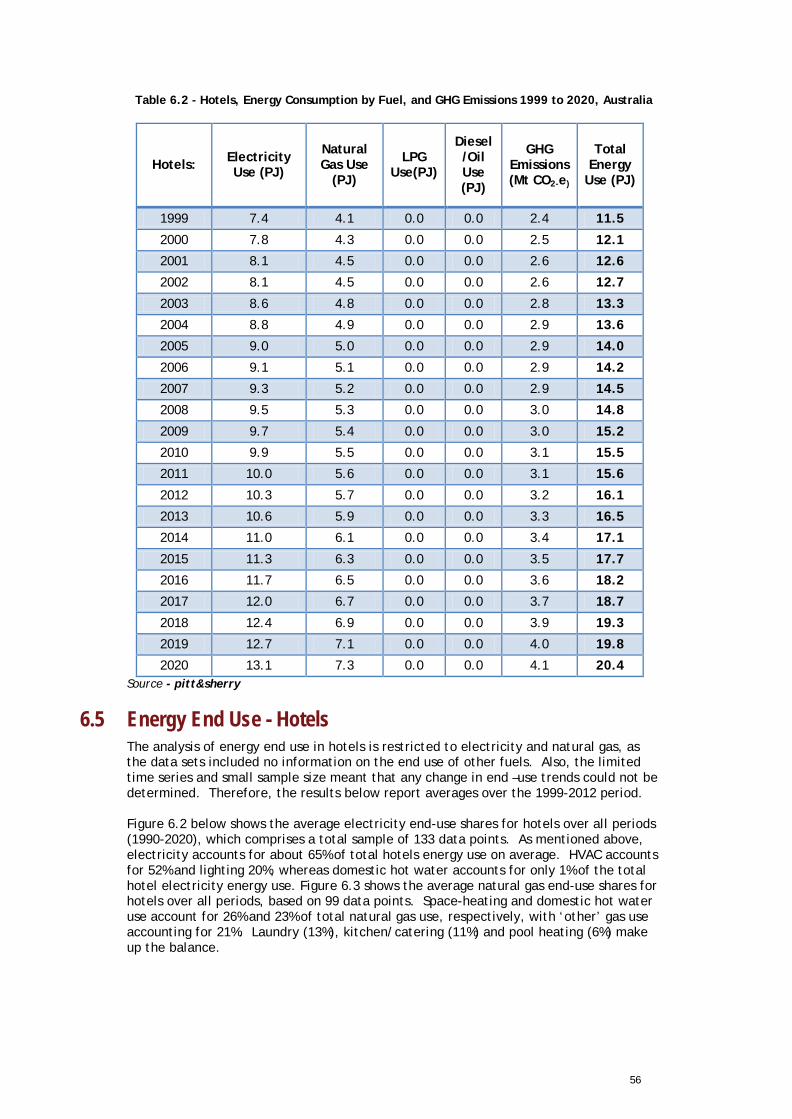
56

Table 6.2 - Hotels, Energy Consumption by Fuel, and GHG Emissions 1999 to 2020, Australia

Hotels: Electricity Use (PJ)

Natural Gas Use

(PJ)

LPG Use(PJ)

Diesel/Oil Use (PJ)

GHG Emissions (Mt CO2-e)

Total Energy

Use (PJ)

1999 7.4 4.1 0.0 0.0 2.4 11.5

2000 7.8 4.3 0.0 0.0 2.5 12.1

2001 8.1 4.5 0.0 0.0 2.6 12.6

2002 8.1 4.5 0.0 0.0 2.6 12.7

2003 8.6 4.8 0.0 0.0 2.8 13.3

2004 8.8 4.9 0.0 0.0 2.9 13.6

2005 9.0 5.0 0.0 0.0 2.9 14.0

2006 9.1 5.1 0.0 0.0 2.9 14.2

2007 9.3 5.2 0.0 0.0 2.9 14.5

2008 9.5 5.3 0.0 0.0 3.0 14.8

2009 9.7 5.4 0.0 0.0 3.0 15.2

2010 9.9 5.5 0.0 0.0 3.1 15.5

2011 10.0 5.6 0.0 0.0 3.1 15.6

2012 10.3 5.7 0.0 0.0 3.2 16.1

2013 10.6 5.9 0.0 0.0 3.3 16.5

2014 11.0 6.1 0.0 0.0 3.4 17.1

2015 11.3 6.3 0.0 0.0 3.5 17.7

2016 11.7 6.5 0.0 0.0 3.6 18.2

2017 12.0 6.7 0.0 0.0 3.7 18.7

2018 12.4 6.9 0.0 0.0 3.9 19.3

2019 12.7 7.1 0.0 0.0 4.0 19.8

2020 13.1 7.3 0.0 0.0 4.1 20.4 Source - pitt&sherry

6.5 Energy End Use - Hotels The analysis of energy end use in hotels is restricted to electricity and natural gas, as the data sets included no information on the end use of other fuels. Also, the limited time series and small sample size meant that any change in end –use trends could not be determined. Therefore, the results below report averages over the 1999-2012 period.

Figure 6.2 below shows the average electricity end-use shares for hotels over all periods (1990-2020), which comprises a total sample of 133 data points. As mentioned above, electricity accounts for about 65% of total hotels energy use on average. HVAC accounts for 52% and lighting 20%, whereas domestic hot water accounts for only 1% of the total hotel electricity energy use. Figure 6.3 shows the average natural gas end-use shares for hotels over all periods, based on 99 data points. Space-heating and domestic hot water use account for 26% and 23% of total natural gas use, respectively, with ‘other’ gas use accounting for 21%. Laundry (13%), kitchen/catering (11%) and pool heating (6%) make up the balance.

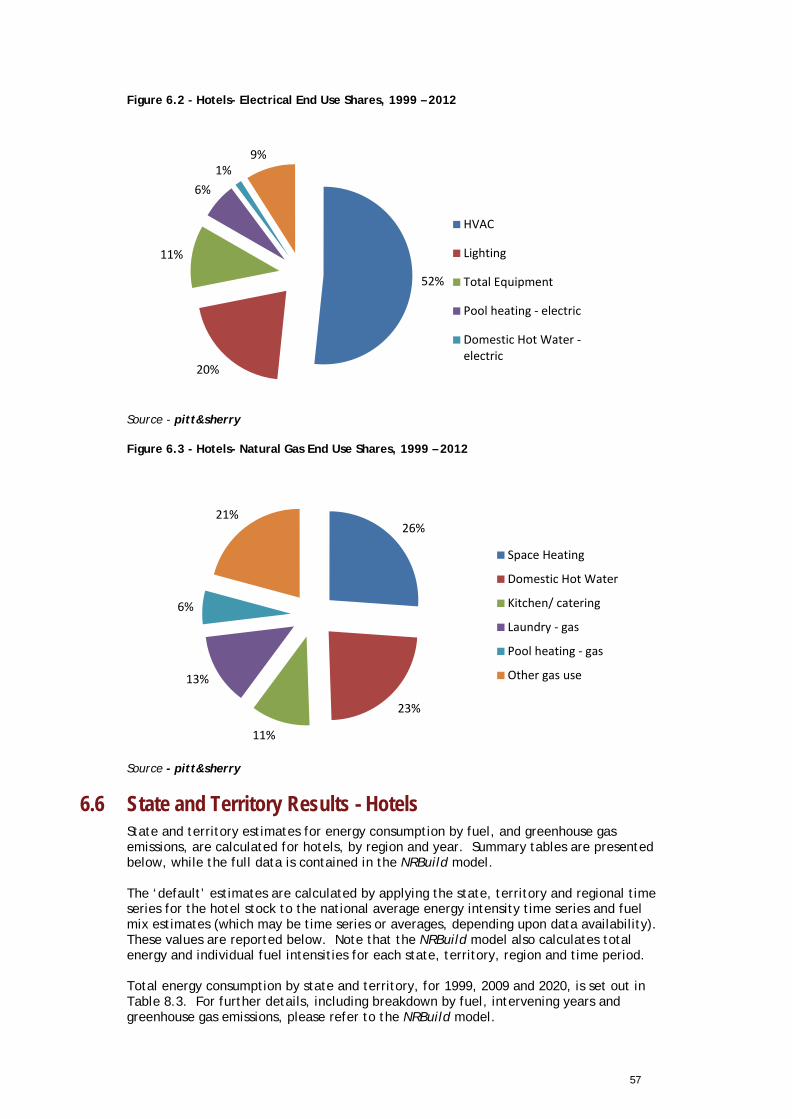
57

Figure 6.2 - Hotels- Electrical End Use Shares, 1999 – 2012

. Source - pitt&sherry Figure 6.3 - Hotels- Natural Gas End Use Shares, 1999 – 2012

. Source - pitt&sherry

6.6 State and Territory Results - Hotels State and territory estimates for energy consumption by fuel, and greenhouse gas emissions, are calculated for hotels, by region and year. Summary tables are presented below, while the full data is contained in the NRBuild model. The ‘default’ estimates are calculated by applying the state, territory and regional time series for the hotel stock to the national average energy intensity time series and fuel mix estimates (which may be time series or averages, depending upon data availability). These values are reported below. Note that the NRBuild model also calculates total energy and individual fuel intensities for each state, territory, region and time period. Total energy consumption by state and territory, for 1999, 2009 and 2020, is set out in Table 8.3. For further details, including breakdown by fuel, intervening years and greenhouse gas emissions, please refer to the NRBuild model.

52%

20%

11%

6% 1%

9%

HVAC

Lighting

Total Equipment

Pool heating - electric

Domestic Hot Water -electric

26%

23%

11%

13%

6%

21%

Space Heating

Domestic Hot Water

Kitchen/ catering

Laundry - gas

Pool heating - gas

Other gas use

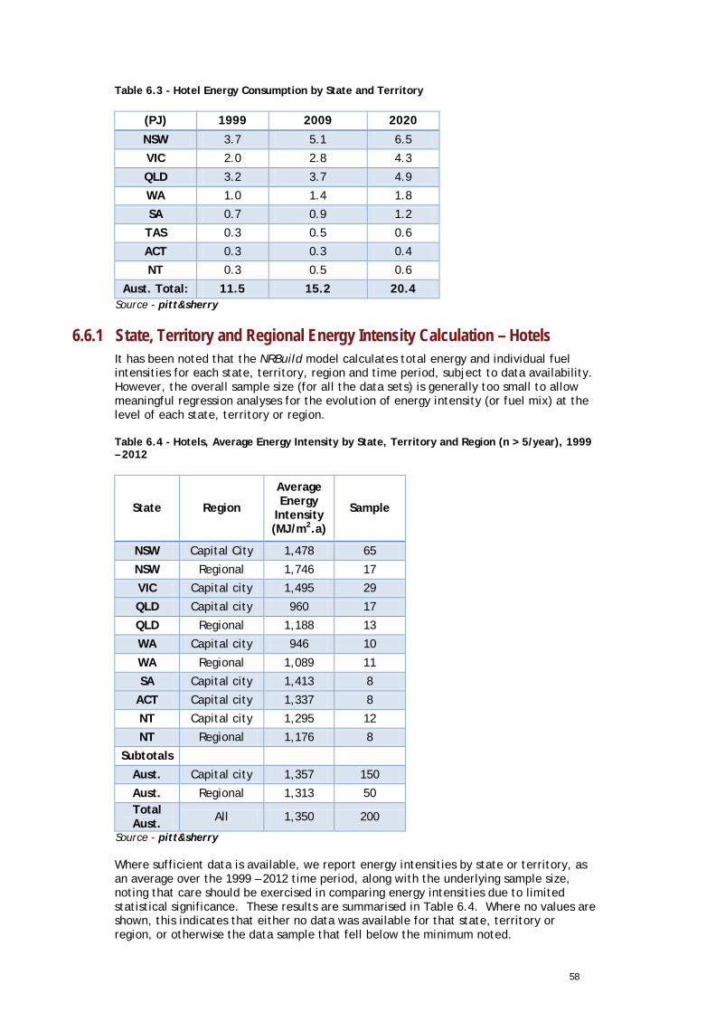
58

Table 6.3 - Hotel Energy Consumption by State and Territory

(PJ) 1999 2009 2020

NSW 3.7 5.1 6.5

VIC 2.0 2.8 4.3

QLD 3.2 3.7 4.9

WA 1.0 1.4 1.8

SA 0.7 0.9 1.2

TAS 0.3 0.5 0.6

ACT 0.3 0.3 0.4

NT 0.3 0.5 0.6

Aust. Total: 11.5 15.2 20.4 Source - pitt&sherry

6.6.1 State, Territory and Regional Energy Intensity Calculation – Hotels It has been noted that the NRBuild model calculates total energy and individual fuel intensities for each state, territory, region and time period, subject to data availability. However, the overall sample size (for all the data sets) is generally too small to allow meaningful regression analyses for the evolution of energy intensity (or fuel mix) at the level of each state, territory or region. Table 6.4 - Hotels, Average Energy Intensity by State, Territory and Region (n > 5/year), 1999 – 2012

State Region

Average Energy

Intensity (MJ/m2.a)

Sample

NSW Capital City 1,478 65

NSW Regional 1,746 17

VIC Capital city 1,495 29

QLD Capital city 960 17

QLD Regional 1,188 13

WA Capital city 946 10

WA Regional 1,089 11

SA Capital city 1,413 8

ACT Capital city 1,337 8

NT Capital city 1,295 12

NT Regional 1,176 8

Subtotals Aust. Capital city 1,357 150

Aust. Regional 1,313 50 Total Aust. All 1,350 200

Source - pitt&sherry

Where sufficient data is available, we report energy intensities by state or territory, as an average over the 1999 – 2012 time period, along with the underlying sample size, noting that care should be exercised in comparing energy intensities due to limited statistical significance. These results are summarised in Table 6.4. Where no values are shown, this indicates that either no data was available for that state, territory or region, or otherwise the data sample that fell below the minimum noted.

59

As previously noted, the NRBuild model allows the user to test their preferred values for energy intensity over time (after the base year of 2009) and specify their own minimum ‘n’ values. The capital city and regional national averages are very similar at 1,357 MJ/m2 and 1,313 MJ/m2, respectively, however, the sample size for regions is very low (no data for some locations). For the capital cities, WA has the lowest average energy intensity (946 MJ/m2.a) which is about 30% lower than the national average. For regions, the average energy intensity ranges from 1,089 MJ/m2.a (WA) to 1,746 MJ/m2.a (NSW). Note that the statistical confidence in the difference in energy intensities between locations is analysed in Appendix E.

6.7 Conclusions - Hotels This analysis of the energy performance of hotels in Australia is based on a limited data sample of some 208 records, which is close to the minimum sample required for 95% confidence with 10% standard error, but only for a single period and region. It is insufficient for an analysis that aims to resolve 15 regions and 13 time periods. Thus, the key requirement to lift the statistical validity of this analysis is to capture more data.

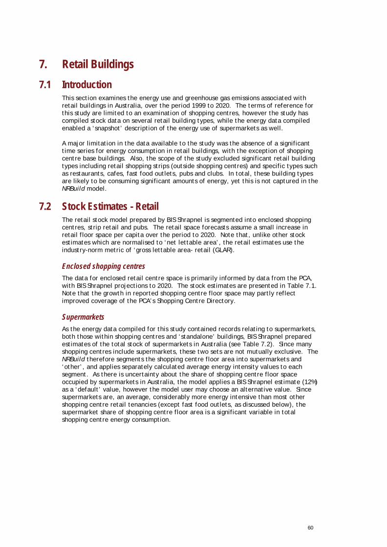
60

7. Retail Buildings 7.1 Introduction

This section examines the energy use and greenhouse gas emissions associated with retail buildings in Australia, over the period 1999 to 2020. The terms of reference for this study are limited to an examination of shopping centres, however the study has compiled stock data on several retail building types, while the energy data compiled enabled a ‘snapshot’ description of the energy use of supermarkets as well. A major limitation in the data available to the study was the absence of a significant time series for energy consumption in retail buildings, with the exception of shopping centre base buildings. Also, the scope of the study excluded significant retail building types including retail shopping strips (outside shopping centres) and specific types such as restaurants, cafes, fast food outlets, pubs and clubs. In total, these building types are likely to be consuming significant amounts of energy, yet this is not captured in the NRBuild model.

7.2 Stock Estimates - Retail The retail stock model prepared by BIS Shrapnel is segmented into enclosed shopping centres, strip retail and pubs. The retail space forecasts assume a small increase in retail floor space per capita over the period to 2020. Note that, unlike other stock estimates which are normalised to ‘net lettable area’, the retail estimates use the industry-norm metric of ‘gross lettable area- retail (GLAR).

Enclosed shopping centres The data for enclosed retail centre space is primarily informed by data from the PCA, with BIS Shrapnel projections to 2020. The stock estimates are presented in Table 7.1. Note that the growth in reported shopping centre floor space may partly reflect improved coverage of the PCA’s Shopping Centre Directory.

Supermarkets As the energy data compiled for this study contained records relating to supermarkets, both those within shopping centres and ‘standalone’ buildings, BIS Shrapnel prepared estimates of the total stock of supermarkets in Australia (see Table 7.2). Since many shopping centres include supermarkets, these two sets are not mutually exclusive. The NRBuild therefore segments the shopping centre floor area into supermarkets and ‘other’, and applies separately calculated average energy intensity values to each segment. As there is uncertainty about the share of shopping centre floor space occupied by supermarkets in Australia, the model applies a BIS Shrapnel estimate (12%) as a ‘default’ value, however the model user may choose an alternative value. Since supermarkets are, an average, considerably more energy intensive than most other shopping centre retail tenancies (except fast food outlets, as discussed below), the supermarket share of shopping centre floor area is a significant variable in total shopping centre energy consumption.

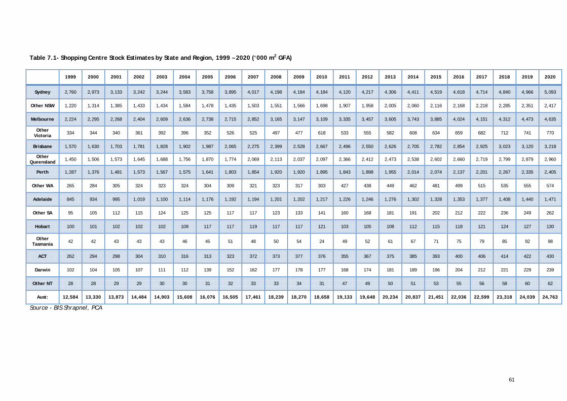
61

Table 7.1- Shopping Centre Stock Estimates by State and Region, 1999 – 2020 (‘000 m2 GFA)

1999 2000 2001 2002 2003 2004 2005 2006 2007 2008 2009 2010 2011 2012 2013 2014 2015 2016 2017 2018 2019 2020

Sydney 2,760 2,973 3,133 3,242 3,244 3,583 3,758 3,895 4,017 4,198 4,184 4,184 4,120 4,217 4,306 4,411 4,519 4,618 4,714 4,840 4,966 5,093

Other NSW 1,220 1,314 1,385 1,433 1,434 1,584 1,478 1,435 1,503 1,551 1,566 1,698 1,907 1,958 2,005 2,060 2,116 2,168 2,218 2,285 2,351 2,417

Melbourne 2,224 2,295 2,268 2,404 2,609 2,636 2,738 2,715 2,852 3,165 3,147 3,109 3,335 3,457 3,605 3,743 3,885 4,024 4,151 4,312 4,473 4,635

Other Victoria 334 344 340 361 392 396 352 526 525 497 477 618 533 555 582 608 634 659 682 712 741 770

Brisbane 1,570 1,630 1,703 1,781 1,828 1,902 1,987 2,065 2,275 2,399 2,528 2,667 2,496 2,550 2,626 2,705 2,782 2,854 2,925 3,023 3,120 3,218

Other Queensland 1,450 1,506 1,573 1,645 1,688 1,756 1,870 1,774 2,069 2,113 2,037 2,097 2,366 2,412 2,473 2,538 2,602 2,660 2,719 2,799 2,879 2,960

Perth 1,287 1,376 1,481 1,573 1,567 1,575 1,641 1,803 1,854 1,920 1,920 1,895 1,843 1,898 1,955 2,014 2,074 2,137 2,201 2,267 2,335 2,405

Other WA 265 284 305 324 323 324 304 309 321 323 317 303 427 438 449 462 481 499 515 535 555 574

Adelaide 845 934 995 1,019 1,100 1,114 1,176 1,192 1,194 1,201 1,202 1,217 1,226 1,246 1,276 1,302 1,328 1,353 1,377 1,408 1,440 1,471

Other SA 95 105 112 115 124 125 125 117 117 123 133 141 160 168 181 191 202 212 222 236 249 262

Hobart 100 101 102 102 102 109 117 117 119 117 117 121 103 105 108 112 115 118 121 124 127 130

Other Tasmania 42 42 43 43 43 46 45 51 48 50 54 24 49 52 61 67 71 75 79 85 92 98

ACT 262 294 298 304 310 316 313 323 372 373 377 376 355 367 375 385 393 400 406 414 422 430

Darwin 102 104 105 107 111 112 139 152 162 177 178 177 168 174 181 189 196 204 212 221 229 239

Other NT 28 28 29 29 30 30 31 32 33 33 34 31 47 49 50 51 53 55 56 58 60 62

Aust: 12,584 13,330 13,873 14,484 14,903 15,608 16,076 16,505 17,461 18,239 18,270 18,658 19,133 19,648 20,234 20,837 21,451 22,036 22,599 23,318 24,039 24,763

Source - BIS Shrapnel, PCA

62

Table 7.2- Supermarket Stock Estimates by State and Region, 1999 – 2020 (‘000 m2 GFA)

1999 2000 2001 2002 2003 2004 2005 2006 2007 2008 2009 2010 2011 2012 2013 2014 2015 2016 2017 2018 2019 2020

Sydney 985 1,007 1,028 1,051 1,074 1,098 1,122 1,146 1,172 1,198 1,225 1,253 1,274 1,300 1,327 1,364 1,401 1,439 1,478 1,516 1,556 1,596

Other NSW 818 833 848 862 878 893 909 925 941 957 973 989 1,000 1,009 1,020 1,031 1,041 1,051 1,061 1,071 1,080 1,090

Melbourne 1,237 1,264 1,292 1,324 1,356 1,387 1,419 1,452 1,486 1,522 1,559 1,596 1,623 1,649 1,677 1,709 1,739 1,769 1,800 1,830 1,861 1,892

Other Victoria 284 291 297 302 306 312 318 324 330 335 339 345 350 354 358 362 366 370 374 378 382 386

Brisbane 572 589 607 626 646 679 698 717 738 761 785 809 822 837 854 874 893 912 933 953 974 994

Other Queensland 576 595 615 636 657 665 689 715 740 764 789 816 830 845 862 881 901 920 938 957 975 993

Perth 546 555 564 575 585 596 606 618 628 639 651 662 676 691 708 728 747 764 783 803 822 842

Other WA 180 183 186 188 190 192 196 198 201 204 206 209 214 218 224 229 234 239 244 248 253 258

Adelaide 410 413 417 421 424 427 430 434 437 441 445 449 452 456 460 466 472 477 483 489 494 500

Other SA 145 147 148 149 150 152 154 155 156 158 159 160 161 163 164 165 167 168 169 171 172 174

Hobart 73 73 74 74 74 75 75 75 76 76 77 77 78 79 80 80 81 82 83 83 84 84

Other Tasmania 98 98 98 98 99 99 99 100 100 100 100 101 101 102 103 103 104 105 105 106 106 107

ACT 117 117 118 118 119 119 120 120 121 121 121 122 123 125 127 128 130 131 133 135 136 138

Darwin 34 35 35 35 35 35 35 36 36 36 36 37 37 38 39 40 41 42 43 44 45 46

Other NT 32 32 32 32 32 32 32 32 32 32 32 32 33 33 34 35 36 37 37 38 39 40

Australia 6,106 6,232 6,360 6,491 6,625 6,762 6,903 7,047 7,194 7,345 7,499 7,657 7,775 7,900 8,036 8,198 8,354 8,507 8,664 8,822 8,980 9,138

Source - BIS Shrapnel

63

Table 7.3 - Retail Strip Stock Estimates by State and Region, 1999 – 2020 (‘000 m2 GFA)

1999 2000 2001 2002 2003 2004 2005 2006 2007 2008 2009 2010 2011 2012 2013 2014 2015 2016 2017 2018 2019 2020

Sydney 6,351 6,321 6,310 6,428 6,620 6,493 6,513 6,706 6,817 6,855 7,047 7,254 7,459 7,514 7,556 7,624 7,701 7,779 7,859 7,937 8,015 8,092

Other NSW 4,401 4,389 4,385 4,406 4,481 4,403 4,601 4,730 4,750 4,883 4,991 4,945 4,819 4,831 4,840 4,858 4,880 4,904 4,928 4,949 4,970 4,990

Melbourne 6,040 6,110 6,302 6,290 6,315 6,466 6,506 6,763 6,856 6,739 7,028 7,450 7,398 7,491 7,552 7,631 7,717 7,778 7,853 7,925 7,997 8,069

Other Victoria 2,994 3,006 3,036 3,037 3,022 3,043 3,122 2,975 3,012 3,088 3,177 3,076 3,221 3,247 3,266 3,290 3,315 3,334 3,357 3,380 3,403 3,426

Brisbane 2,253 2,313 2,314 2,391 2,481 2,518 2,528 2,570 2,549 2,681 2,701 2,646 2,947 3,020 3,055 3,110 3,174 3,241 3,305 3,368 3,431 3,493

Other Queensland 3,388 3,464 3,477 3,494 3,566 3,588 3,593 3,905 3,838 3,916 4,235 4,326 4,213 4,301 4,354 4,429 4,513 4,597 4,679 4,766 4,853 4,940

Perth 2,138 2,169 2,162 2,128 2,196 2,284 2,284 2,187 2,266 2,319 2,455 2,582 2,717 2,766 2,817 2,899 2,977 3,027 3,079 3,160 3,240 3,318

Other WA 914 929 935 945 971 997 1,037 1,064 1,084 1,113 1,149 1,183 1,086 1,106 1,126 1,155 1,177 1,191 1,210 1,233 1,257 1,281

Adelaide 1,864 1,794 1,769 1,771 1,725 1,747 1,736 1,788 1,830 1,860 1,892 1,923 1,941 1,964 1,964 1,976 1,988 1,996 2,008 2,020 2,033 2,045

Other SA 747 744 751 758 763 775 797 816 823 838 853 863 853 857 852 851 851 849 849 848 846 845

Hobart 361 366 370 373 378 376 372 387 391 407 417 416 439 445 451 453 455 456 458 461 464 466

Other Tasmania 610 616 620 624 629 632 641 651 661 667 668 708 688 692 692 691 692 691 692 691 690 690

ACT 420 444 449 454 473 475 484 489 524 537 589 600 647 649 653 658 662 666 673 675 677 680

Darwin 68 76 86 94 107 119 105 107 112 110 118 129 152 149 149 154 158 159 159 160 160 160

Other NT 112 119 129 137 147 155 160 166 172 185 194 214 209 211 214 222 229 233 237 242 247 251

Australia: 32,659 32,862 33,095 33,328 33,873 34,072 34,481 35,305 35,683 36,199 37,515 38,316 38,789 39,242 39,542 40,002 40,489 40,902 41,345 41,816 42,283 42,746

Source - BIS Shrapnel

64

Strip retail, pubs ‘Strip retail’ floor area is calculated by taking total BIS estimates of total retail (excluding pubs) and subtracting enclosed retail centres (see Table 7.3). Total retail space is estimated by applying a ratio of around 2.5 m2 to 2.6m2 per capita. This ratio is higher than those typically used by retail industry analysts because the definition of total retail space used here is broader than that typically used by retail analysts. For example, it includes an allowance of around 0.3m2 per capita for office services provided in ‘retail’ space (such as real estate agents) and motor vehicle retail – the exact ratio used varies between centres. Pubs fall within the retail classification, although they are outside the terms of reference for this study. Neverthless we have developed separate stock estimates of pub space as a sub-classification. The estimates are of a low quality, being based on a small sample of hard data for the Sydney and Melbourne Local Government Authorities (LGAs), and then using space per person employed as a proxy to create estimates for space in other parts of the country. Limitations of using employment as a metric include the different opening hours of pubs and significant part/time casual workforce. We have assumed that there is an average of 45m2 per pub employee. Note that the energy performance of these buildings is not modelled, as they fell outside the study’s terms of reference, however the stock estimates compiled provide a starting point for the development of additional model segments for these building types in the future. As noted, the stock estimates are not mutually exclusive, as supermarkets may be found both in shopping centres and retail shopping strips. We estimate that, on average, some 22% of shopping centre floor area is occupied by supermarkets. The balance of the supermarket stock is assumed to be ‘standalone’ buildings.

7.3 Energy Intensity - Retail There was insufficient energy consumption data available for this study to make a robust analysis of energy performance trends in the retail sector at the degree of resolution desired – particularly over the historical period back to 1999. While the study captured a total of 1,980 records relating to 1,052 individual buildings in the sector, this data was heavily weighted towards the 2011 financial year and also unevenly distributed by building type. Some time series data was available for shopping centre base buildings (172 records), but insufficient for statistically valid analysis when disaggregated by year, state and region. For this reason, the analysis of the energy performance of the retail stock largely represents a ‘snapshot’ in time. Further targeted data capture would be required to populate a time series model, as recommended in Section 7.8 below. Energy intensity and fuel mix ‘default’ estimates are therefore simple averages of the data available. As for other building types, the NRBuild model enables the user to specify alternative values for energy intensity and fuel mix, including projections over the period to 2020. Despite this limitation, the study has enabled useful comparative analysis of the energy intensity of different retail building types. This, in addition to the stock estimates, should help target future research.

Hours of Operation As noted in Section 3.2 above, the retail energy data sets were normalised for hours of operation. Average values for hours of operation were calculated from those records that revealed this information, while those that did not reveal any values for hours of operation were assumed to have the average value. Reported fuel consumption for each record was then factored up or down as a function of the ratio of average hours to reported hours. As a result, the reported values for energy intensity may be directly compared. For all shopping centre retail areas, the average value for hours of operation was just over 79 hours per week. However, this segmented into an average of over 96 hours/week for supermarkets located in shopping centres, and just over 59 hours/week for other retail tenancies.

65

For base and whole buildings, average values for hours of operation were just over 61 hours/week for shopping centres and almost 100 hours/week for supermarkets.

7.3.1 Energy Intensity - Shopping Centres Shopping centre energy intensity estimates are sub-divided into tenancies (supermarkets and others), base buildings and whole buildings.

Retail Tenancies 853 data records relating to retail tenancies (other than supermarkets) were collated, representing just under 200,000 m2 of retail space. These records related primarily to 2010 (638 records) and 2011 (215 records). By contrast, most states and regions are covered by this data, with the exceptions of Perth, Hobart and Darwin. The tenancy types vary from fast food outlets and cafes (in shopping centres), to large-surface general retailers and micro-sized specialty shops and include many of the most common retail chains represented across Australia. The average size of these tenancies is 229 m2 GLAR, although the median (or central) value is just 97 m2 GLAR. The average energy intensity of this sample was 915 MJ/m2a. As with other such calculations, the average value represents the area-weighted average of all states and regions. Given the limited overall data sample, there are few significant estimates available for energy intensity at the state, territory or regional level. However, it appears that the average energy intensity of retail tenancies in capital cities is some 13% higher than those in regional areas, at around 960 MJ/m2.a as compared to around 850 MJ/m2.a in regional areas. Significant average values are recorded for Brisbane (1,011 MJ/m2.a; n=517) and regional Queensland (881 MJ/m2.a; n=310) only. Not surprisingly, given likely climate effects, these values are modestly higher than the national averages. When the retail tenancy energy intensity values were sorted from highest to lowest, it was immediately apparent that the most energy intensive retail tenancies (in shopping centres) are fast food outlets. These outlets typically occupy a limited floor area (including the ‘hole in the wall’ variety, eg, less than 10 m2 GLAR) yet feature significant cooking, heating, display lighting and refrigeration – all energy intensive processes. As a result, energy intensities as high as 48,000 MJ/m2.a are revealed in the data set, with values near or above 10,000 MJ/m2.a reasonably common. Note that the skewed distribution of energy intensities within the sample (and, most likely, within the actual retail stock) highlights the value of area-weighted averages. Examining the set of all shopping centres tenancies, for example, shows an area-weighted average energy intensity of 915 MJ/m2.a, as noted above, but a simple or unweighted average value of 1,550 MJ/m2.a, some 41% higher. The latter value over-estimates the average energy performance of the retail stock, as it is skewed towards the smaller area of very high energy-intensity retailers, such as the fast food outlets noted.

Base Buildings Turning to retail shopping centre base buildings, the data set comprises 172 records. The data covers the period 2007 to 2011, and the average values reported below are averages over these 5 years. The average floor area associated with these records is substantially larger than for the retail tenancies, at almost 12,700 m2 GFA, while the media floor area is around 2,750 m2 GLAR. This indicates that the sample includes a smaller number of large shopping centres and a larger number of smaller ones. Based on this data, the national average energy intensity value for shopping centre base buildings is just over 400 MJ/m2.a. As with the retail tenancies, the average energy intensity of capital city shopping centre base buildings appears higher than those in regional areas, at almost 450 MJ/m2.a for capital cities on average (n=82), as compared

66

with around 350 MJ/m2.a for regional areas (n=90). Given the modest overall sample, no significant intensity values are reported by state and territory.

Whole Buildings Records relating to shopping centre whole buildings were limited to just 35, albeit that they covered more than 1.1 million m2 GLAR. They relate to the years 2007 – 2011. This set was judged too small for valid statistical analysis, and therefore – as with offices - ‘whole building’ calculations represent the sum of base buildings plus retail tenancies. As noted above, the retail tenancy energy intensity values represent the area-weighted average of supermarket and other retail types. On this basis, and assuming 12% of shopping centre floor area is represented by supermarkets, the national average energy intensity of whole shopping centres is just over 1,600 MJ/m2.a. This result is sensitive to the assumption for supermarket area, as supermarket tenancies are considerably more energy intensive than the average retail tenancy (as discussed further below). This value may be varied by the user in the NRBuild model, within reason, noting that any value above about 40% (supermarket share of shopping centre floor area) would imply that all supermarkets in Australia were located in shopping centres.

7.3.2 Energy Intensity - Supermarkets Some 839 data records were compiled for supermarkets, comprising 594 whole building observations and 245 supermarket retail tenancies (i.e, those located in shopping centres). The data relates almost exclusively to financial year 2011 and represents a total of over 2 million m2 GFA. The sample is reasonably broadly distributed by state and region, with no data on supermarket tenancies for Hobart and regional NT (where the stock of supermarkets in shopping centres is likely to be limited in any case), and with limited data for supermarket whole buildings in Perth (n=1), Darwin (n=2) and Hobart (n=4). Beginning with the supermarkets within shopping centres, the area-weighted national average energy intensity of these supermarkets was just over 3,300 MJ/m2.a, while the simple average value was less than 2% higher at around 3,370 MJ/m2.a, suggesting a reasonably uniform distribution of intensity values within the sample. In contrast to general retail tenancies, the average energy intensity of supermarkets in shopping centres in regional areas was higher (at around 3,520 MJ/m2.a; n=101) compared with those in capital cities (at around 3,150 MJ/m2.a; n=144). At the level of states and territories, the cooler climates appear to show lower energy intensities, such around 2,600 MJ/m2.a for Melbourne, regional Victoria and the ACT; and just under 3,000 MJ/m2.a for regional Tasmania. While no end-use breakdowns were available for retail buildings, we note that supermarket energy consumption is dominated firstly by space cooling needs, and then by refrigeration and lighting, which in turn create further space cooling needs. Therefore the cooler climates have a natural advantage in this regard. By contrast, the highest energy intensity values (for supermarkets in shopping centres) are found in the warmer climates of WA (close to 3,900 MJ/m2.a; n=37) and QLD (over 3,600 MJ/m2.a in Brisbane, n=47; and over 3,800 MJ/m2.a in regional Queensland, n=24). Only one data point was available for Darwin, and this was over 3,900 MJ/m2.a.

Turning to standalone supermarkets, the national average energy intensity was 3,375 MJ/m2.a, with a similar pattern of slightly higher averages in regional areas (around 3,560 MJ/m2.a, n=276) when compared with capital cities (around 3,200 MJ/m2.a, n=318). Likewise, the higher average energy intensity values are found in the warmer regions, such as over 4,600 MJ/m2.a in regional QLD (n=46), and close to 4,100 in regional WA (n=47); while the cooler climate show lower average values, including around 2,600 MJ/m2.a for Melbourne (n=104), around 2,900 MJ/m2.a for regional Victoria (n=52) and regional SA (n=16), and around 3,000 MJ/m2.a for regional Tasmania (n=21).

67

Note that the statistical confidence in the difference in energy intensities between locations is analysed in Appendix E.

7.4 Total Energy Consumption and Greenhouse Gas Emissions - Retail

7.4.1 All Retail Table 7.4 shows that total energy use in the retail buildings covered by the study is estimated to have been some 47.2 PJ in the base year of 2009. Table 7.4 - Retail: Energy Use and Greenhouse Gas Emissions, 1999 – 2020

Shopping Centres (Total)

Shopping Centres (Base

Building)

Shopping Centres

(Tenancies)

Supermarkets (Total)

Supermarkets (Stand Alone) TOTALS

Total Energy

Use

GHG (Mt

CO2-e)

Total Energy

Use

GHG (Mt

CO2-e)

Total Energy

Use

GHG (Mt

CO2-e)

Total Energy

Use

GHG (Mt

CO2-e)

Total Energy

Use

GHG (Mt CO2-

e)

Total Energy

Use (PJ)

GHG Emissions (Mt CO2-e)

1999 - - 5.1 1.4 - - - - - - - -

2000 - - 5.4 1.5 - - - - - - - -

2001 - - 5.6 1.6 - - - - - - - -

2002 - - 5.8 1.6 - - - - - - - -

2003 - - 6.0 1.7 - - - - - - - -

2004 - - 6.3 1.8 - - - - - - - -

2005 - - 6.5 1.8 - - - - - - - -

2006 - - 6.7 1.8 - - - - - - - -

2007 - - 7.0 1.9 - - - - - - - -

2008 - - 7.3 2.0 - - - - - - - -

2009 29.3 8.3 7.4 2.0 22.0 6.3 25.3 7.3 17.9 5.1 47.2 13.4

2010 29.9 8.4 7.5 2.0 22.4 6.4 25.8 7.4 18.3 5.2 48.2 13.6

2011 30.7 8.6 7.7 2.1 23.0 6.5 26.2 7.5 18.6 5.3 49.3 13.9

2012 31.5 8.8 7.9 2.1 23.6 6.7 26.7 7.6 18.9 5.4 50.4 14.2

2013 32.5 9.1 8.2 2.2 24.3 6.9 27.1 7.7 19.2 5.5 51.7 14.6

2014 33.4 9.4 8.4 2.3 25.0 7.1 27.7 7.9 19.6 5.6 53.0 15.0

2015 34.4 9.7 8.6 2.3 25.8 7.3 28.2 8.0 20.0 5.7 54.4 15.4

2016 35.4 9.9 8.9 2.4 26.5 7.5 28.7 8.2 20.3 5.8 55.7 15.7

2017 36.3 10.2 9.1 2.5 27.2 7.7 29.2 8.3 20.7 5.9 57.0 16.1

2018 37.4 10.5 9.4 2.5 28.0 8.0 29.8 8.5 21.1 6.0 58.5 16.5

2019 38.6 10.8 9.7 2.6 28.9 8.2 30.3 8.6 21.4 6.1 60.0 17.0

2020 39.7 11.2 10.0 2.7 29.8 8.5 30.8 8.8 21.8 6.2 61.6 17.4 Source - pitt&sherry Notes: No statistically significant data on the energy consumption of supermarkets or shopping centres tenancies was available prior to 2009. 'Shopping Centres (Total)' includes supermarkets inside shopping centres. Supermarkets in shopping centres are included in 'Shopping Centres (Tenancies)'. 'Supermarkets (Total)' represents the all supermarkets, including those in shopping centres, while 'Supermarkets (Standalone)' are net of those in shopping centres.

Greenhouse gas emissions associated with this energy use are estimated at 13.4 Mt CO2-e. By 2020, energy consumption in these buildings is expected to increase by a substantial 32% over this 2009 base, to around 62 PJ, while greenhouse gas emissions are

68

expected to reach 17.4 Mt CO2-e in the same year. Since the study assumes constant energy intensity in these buildings over the forecast period, and also a constant fuel mix (as a result of the data limitations noted above), these projections reflect expected growth trends in the building stock, as described in Section 7.2 above. No attempt was made to backcast energy consumption in periods prior to the base year, given the lack of the energy intensity data for period back to 1999. Significant additional data capture would be required populate the retail building modules in NRBuild model back to 1999.

7.4.2 Shopping Centres Table 7.4 also shows that estimated energy consumption in shopping centres in the base year of 2009 was around 29.3 PJ, with the majority of this energy use (22 PJ) attributable to retail tenancies – including an assumption of 12% supermarket floor area within shopping centres, with the balance (around 7.4 PJ) attributable to base building energy consumption. Note that these estimates include the energy attributable to the estimated 12% of shopping centre floor area occupied by supermarkets. These values are expected to increase, in line with growth in the underlying building stock, to just under 40 PJ in 2020 in total, with around 30 PJ attributable to tenancies and the balance to base buildings. In terms of greenhouse gas emissions, we estimate around 8.3 Mt CO2-e for all shopping centres in 2009, with around 8.3 Mt CO2-e attributable to tenancies, and some 11.2 Mt CO2-e in 2020, of which around 8.5 Mt CO2-e is attributable to tenancies. As noted earlier, there is uncertainty about the area of supermarkets within shopping centres in Australia: values higher than the assumed 12% would tend to increase estimates for total energy and greenhouse gas emissions. We would characterise the estimates for 2009 as ‘medium’ confidence, while the projections for 2020 are ‘low’ confidence, given the data limitations described above.

Fuel Mix Noting the data limitations above, only an average fuel mix observations were available for shopping centres, rather than time series. Taking all shopping centres as a whole, the average fuel mix is dominated by electricity at around 97.5%, with the balance accounted for by natural gas. Within shopping centre tenancies, electricity’s share on average is even higher, at over 99% (natural gas is the balance). Implied in these results is a somewhat lower electricity share for shopping centre base buildings, which we estimate at just under 93% on average, with the balance attributable to natural gas. No significant use of diesel or LPG was noted. No statistically significant end use information was available in this data set, however it is likely that the modest amounts of gas consumed in shopping centres are associated with space heating, cooking and domestic hot water applications.

7.4.3 Supermarkets Supermarket energy consumption and greenhouse gas emissions are presented for ‘standalone’ supermarkets (those outside shopping centres) and all supermarkets (including those inside shopping centres). The latter estimates may therefore not be added to the shopping centre estimates, as this would double count the supermarkets in shopping centres. Table 7.4 shows that we estimate total supermarket energy consumption in 2009 to have been around 25.3 PJ, of which around 17.9 PJ is estimated to have been consumed in standalone supermarkets, and the balance in supermarkets in shopping centres. Total supermarket energy consumption is projected to increase by some 22% to 2020, reaching almost 31 PJ, of which almost 22 PJ is attributable to standalone supermarkets. In terms of greenhouse gas emissions, total emissions associated with supermarkets are estimated at around 7.3 Mt CO2-e in 2009, of which just over 5 PJ is attributable to the standalone supermarkets. By 2020, these values are expected to increase to around 8.8

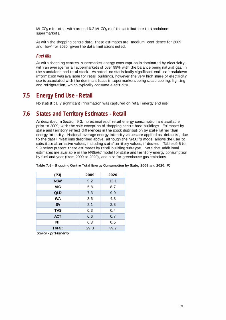
69

Mt CO2-e in total, with around 6.2 Mt CO2-e of this attributable to standalone supermarkets. As with the shopping centre data, these estimates are ‘medium’ confidence for 2009 and ‘low’ for 2020, given the data limitations noted.

Fuel Mix As with shopping centres, supermarket energy consumption is dominated by electricity, with an average for all supermarkets of over 99%, with the balance being natural gas, in the standalone and total stock. As noted, no statistically significant end-use breakdown information was available for retail buildings, however the very high share of electricity use is associated with the dominant loads in supermarkets being space cooling, lighting and refrigeration, which typically consume electricity.

7.5 Energy End Use - Retail No statistically significant information was captured on retail energy end use.

7.6 States and Territory Estimates - Retail As described in Section 9.3, no estimates of retail energy consumption are available prior to 2009, with the sole exception of shopping centre base buildings. Estimates by state and territory reflect differences in the stock distribution by state rather than energy intensity. National average energy intensity values are applied as ‘defaults’, due to the data limitations described above, although the NRBuild model allows the user to substitute alternative values, including state/territory values, if desired. Tables 9.5 to 9.9 below present these estimates by retail building sub-type. Note that additional estimates are available in the NRBuild model for state and territory energy consumption by fuel and year (from 2009 to 2020), and also for greenhouse gas emissions.

Table 7.5 - Shopping Centre Total Energy Consumption by State, 2009 and 2020, PJ

(PJ) 2009 2020

NSW 9.2 12.1

VIC 5.8 8.7

QLD 7.3 9.9

WA 3.6 4.8

SA 2.1 2.8

TAS 0.3 0.4

ACT 0.6 0.7

NT 0.3 0.5

Total: 29.3 39.7 Source - pitt&sherry

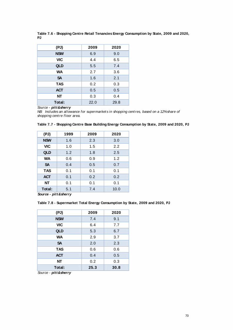
70

Table 7.6 - Shopping Centre Retail Tenancies Energy Consumption by State, 2009 and 2020, PJ

(PJ) 2009 2020

NSW 6.9 9.0

VIC 4.4 6.5

QLD 5.5 7.4

WA 2.7 3.6

SA 1.6 2.1

TAS 0.2 0.3

ACT 0.5 0.5

NT 0.3 0.4

Total: 22.0 29.8 Source - pitt&sherry NB: Includes an allowance for supermarkets in shopping centres, based on a 12% share of shopping centre floor area.

Table 7.7 - Shopping Centre Base Building Energy Consumption by State, 2009 and 2020, PJ

(PJ) 1999 2009 2020

NSW 1.6 2.3 3.0

VIC 1.0 1.5 2.2

QLD 1.2 1.8 2.5

WA 0.6 0.9 1.2

SA 0.4 0.5 0.7

TAS 0.1 0.1 0.1

ACT 0.1 0.2 0.2

NT 0.1 0.1 0.1

Total: 5.1 7.4 10.0 Source - pitt&sherry

Table 7.8 - Supermarket Total Energy Consumption by State, 2009 and 2020, PJ

(PJ) 2009 2020

NSW 7.4 9.1

VIC 6.4 7.7

QLD 5.3 6.7

WA 2.9 3.7

SA 2.0 2.3

TAS 0.6 0.6

ACT 0.4 0.5

NT 0.2 0.3

Total: 25.3 30.8 Source - pitt&sherry

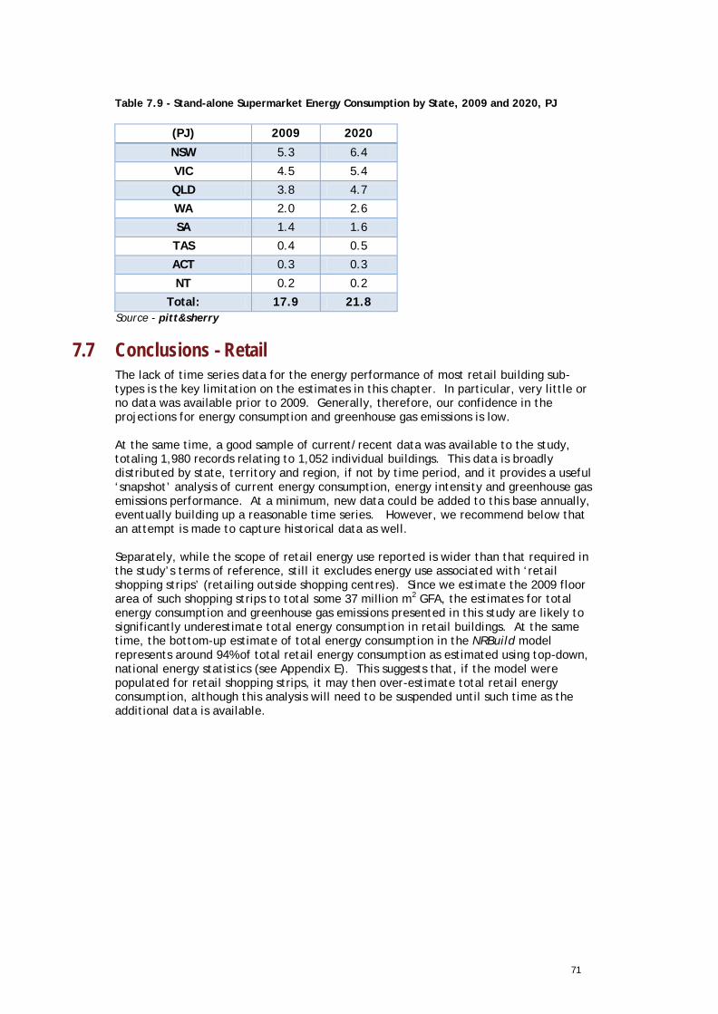
71

Table 7.9 - Stand-alone Supermarket Energy Consumption by State, 2009 and 2020, PJ

(PJ) 2009 2020

NSW 5.3 6.4

VIC 4.5 5.4

QLD 3.8 4.7

WA 2.0 2.6

SA 1.4 1.6

TAS 0.4 0.5

ACT 0.3 0.3

NT 0.2 0.2

Total: 17.9 21.8 Source - pitt&sherry

7.7 Conclusions - Retail The lack of time series data for the energy performance of most retail building sub-types is the key limitation on the estimates in this chapter. In particular, very little or no data was available prior to 2009. Generally, therefore, our confidence in the projections for energy consumption and greenhouse gas emissions is low. At the same time, a good sample of current/recent data was available to the study, totaling 1,980 records relating to 1,052 individual buildings. This data is broadly distributed by state, territory and region, if not by time period, and it provides a useful ‘snapshot’ analysis of current energy consumption, energy intensity and greenhouse gas emissions performance. At a minimum, new data could be added to this base annually, eventually building up a reasonable time series. However, we recommend below that an attempt is made to capture historical data as well. Separately, while the scope of retail energy use reported is wider than that required in the study’s terms of reference, still it excludes energy use associated with ‘retail shopping strips’ (retailing outside shopping centres). Since we estimate the 2009 floor area of such shopping strips to total some 37 million m2 GFA, the estimates for total energy consumption and greenhouse gas emissions presented in this study are likely to significantly underestimate total energy consumption in retail buildings. At the same time, the bottom-up estimate of total energy consumption in the NRBuild model represents around 94% of total retail energy consumption as estimated using top-down, national energy statistics (see Appendix E). This suggests that, if the model were populated for retail shopping strips, it may then over-estimate total retail energy consumption, although this analysis will need to be suspended until such time as the additional data is available.

72

8. Hospitals 8.1 Introduction

This chapter presents key findings and underlying assumptions for hospitals, as modelled in NRBuild. No energy data was available for private hospitals. Based on the energy data captured for public hospitals/healthcare facilities, average energy intensity figures were calculated which were applied to all (public and private) stock to estimate total energy consumption and greenhouse gas emissions.

8.2 Stock Estimates - Hospitals The stock of hospital space in Australia has been estimated by BIS Shrapnel, drawing on data sources and estimation techniques, as summarised in Chapter 3, with further detail in Appendix C. In the BIS Shrapnel stock model, the healthcare classification is divided into public hospitals, private acute care hospitals, private day hospitals and other health care. However, the NRBuild model only covers the major public and private hospitals, as described below.

Public hospital floor space estimates Floor space estimates for public hospitals are based on data sourced from state and territory health authorities, which have then been adjusted to normalise for definitional differences. In some states, information on the number of hospital beds (as defined by the Australian Institute of Health and Welfare (AIHW)) has been used to proxy public hospital space. The average space is assumed to be around 171m2 per public hospital bed in 2010, although for most states, there was limited information on the capital city/regional split of floor area.

Private hospital floor space estimates Private hospital floor space has been calculated by multiplying the number of beds by assumed m2/ bed. The number of hospital beds is sourced from the AIHW. However, a sample of private hospitals showed wide variation in floor space per bed. For private acute care hospitals, the assumed average space per bed is 100m2 -120m2.

Hospital floor space forecasts The hospital floor space forecasts are based on several factors, including information on existing projects. Other factors include estimates for the number of patient days. Data on patient days per population by 5 year age group is available from the AIHW. This data is combined with forecasts for population by 5 year age group to produce an estimate of the trend in the number of patient days based purely on demographic factors. This figure is then adjusted qualitatively to take account of the fact that improved medical procedures should result in shorter hospital stays over time and likely funding constraints for hospital construction. In the base year of 2009, hospitals are estimated to have comprised some 12.4 million m2 across Australia as a whole (see Table 8.1). Historically, the stock growth fluctuated between 1999 and 2011, with stock numbers actually decreasing in some years as a result of demolitions and subsequent rebuilds. However from 2009, it projected to grow to 2020 at around 2% per year. New South Wales comprises the largest share of all hospital stock by state/territory, however, this share is expected to fall slightly over the 2009 to 2020 period, from 32.8% to 32.3%. Over the same period, the shares of Queensland and Western Australia are expected to increase, from 20% to 21% (QLD) and from 12.2% to 13.3% (WA).

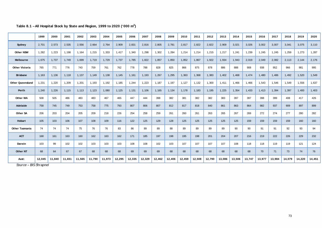
73

Table 8.1 – All Hospital Stock by State and Region, 1999 to 2020 (‘000 m2)

1999 2000 2001 2002 2003 2004 2005 2006 2007 2008 2009 2010 2011 2012 2013 2014 2015 2016 2017 2018 2019 2020

Sydney 2,701 2,573 2,535 2,556 2,664 2,764 2,909 2,831 2,816 2,805 2,781 2,817 2,822 2,822 2,909 3,021 3,026 3,002 3,007 3,041 3,075 3,110

Other NSW 1,282 1,223 1,198 1,164 1,215 1,333 1,417 1,340 1,298 1,302 1,284 1,214 1,214 1,215 1,217 1,241 1,239 1,245 1,245 1,259 1,273 1,287

Melbourne 1,675 1,737 1,749 1,699 1,719 1,729 1,737 1,785 1,822 1,857 1,850 1,852 1,867 1,922 1,934 1,943 2,019 2,049 2,082 2,113 2,144 2,176

Other Victoria 765 771 776 743 759 761 762 778 788 828 825 866 875 878 886 888 908 938 952 966 981 995

Brisbane 1,163 1,136 1,118 1,137 1,149 1,138 1,145 1,161 1,193 1,267 1,295 1,363 1,368 1,383 1,402 1,468 1,474 1,480 1,486 1,492 1,520 1,549

Other Queensland 1,231 1,220 1,209 1,201 1,193 1,192 1,185 1,244 1,223 1,187 1,197 1,127 1,132 1,300 1,411 1,466 1,466 1,543 1,546 1,549 1,556 1,637

Perth 1,240 1,226 1,115 1,113 1,123 1,080 1,125 1,131 1,106 1,165 1,134 1,178 1,183 1,195 1,225 1,354 1,433 1,413 1,394 1,397 1,400 1,403

Other WA 508 505 486 483 483 467 465 447 444 398 382 381 382 382 383 397 397 398 399 408 417 426

Adelaide 758 745 749 753 758 775 793 807 806 807 812 817 818 840 861 863 864 982 937 909 897 899

Other SA 206 203 204 205 209 218 226 254 258 259 261 260 261 263 265 267 269 272 274 277 280 282

Hobart 105 103 106 107 108 109 116 122 125 129 128 125 125 125 125 125 159 159 159 159 160 160

Other Tasmania 74 74 74 75 76 76 83 86 89 89 88 89 89 89 89 90 90 91 91 92 93 94

ACT 168 161 163 160 162 163 162 171 185 197 198 195 198 201 204 207 216 219 222 226 229 232

Darwin 103 99 102 102 103 103 103 108 108 102 103 107 107 107 107 108 118 118 119 119 121 124

Other NT 68 64 67 67 68 68 68 69 69 69 68 68 68 68 68 68 68 70 71 73 74 76

Aust: 12,045 11,840 11,651 11,565 11,790 11,973 12,295 12,335 12,329 12,462 12,406 12,459 12,508 12,790 13,086 13,506 13,747 13,977 13,984 14,079 14,220 14,451

Source - BIS Shrapnel

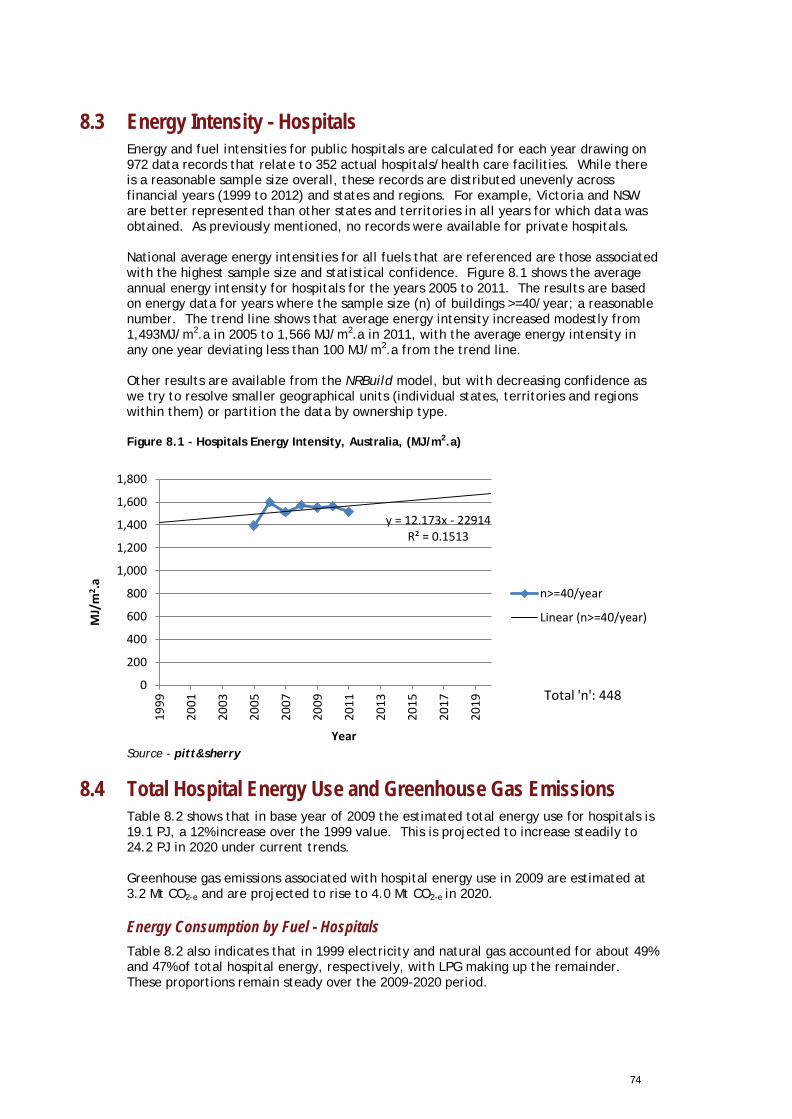
74

8.3 Energy Intensity - Hospitals Energy and fuel intensities for public hospitals are calculated for each year drawing on 972 data records that relate to 352 actual hospitals/health care facilities. While there is a reasonable sample size overall, these records are distributed unevenly across financial years (1999 to 2012) and states and regions. For example, Victoria and NSW are better represented than other states and territories in all years for which data was obtained. As previously mentioned, no records were available for private hospitals. National average energy intensities for all fuels that are referenced are those associated with the highest sample size and statistical confidence. Figure 8.1 shows the average annual energy intensity for hospitals for the years 2005 to 2011. The results are based on energy data for years where the sample size (n) of buildings >=40/year; a reasonable number. The trend line shows that average energy intensity increased modestly from 1,493MJ/m2.a in 2005 to 1,566 MJ/m2.a in 2011, with the average energy intensity in any one year deviating less than 100 MJ/m2.a from the trend line. Other results are available from the NRBuild model, but with decreasing confidence as we try to resolve smaller geographical units (individual states, territories and regions within them) or partition the data by ownership type. Figure 8.1 - Hospitals Energy Intensity, Australia, (MJ/m2.a)

..

Source - pitt&sherry

8.4 Total Hospital Energy Use and Greenhouse Gas Emissions Table 8.2 shows that in base year of 2009 the estimated total energy use for hospitals is 19.1 PJ, a 12% increase over the 1999 value. This is projected to increase steadily to 24.2 PJ in 2020 under current trends. Greenhouse gas emissions associated with hospital energy use in 2009 are estimated at 3.2 Mt CO2-e and are projected to rise to 4.0 Mt CO2-e in 2020.

Energy Consumption by Fuel - Hospitals Table 8.2 also indicates that in 1999 electricity and natural gas accounted for about 49% and 47% of total hospital energy, respectively, with LPG making up the remainder. These proportions remain steady over the 2009-2020 period.

y = 12.173x - 22914 R² = 0.1513

0

200

400

600

800

1,000

1,200

1,400

1,600

1,800

1999

2001

2003

2005

2007

2009

2011

2013

2015

2017

2019

MJ/

m2 .a

Year

n>=40/year

Linear (n>=40/year)

Total 'n': 448

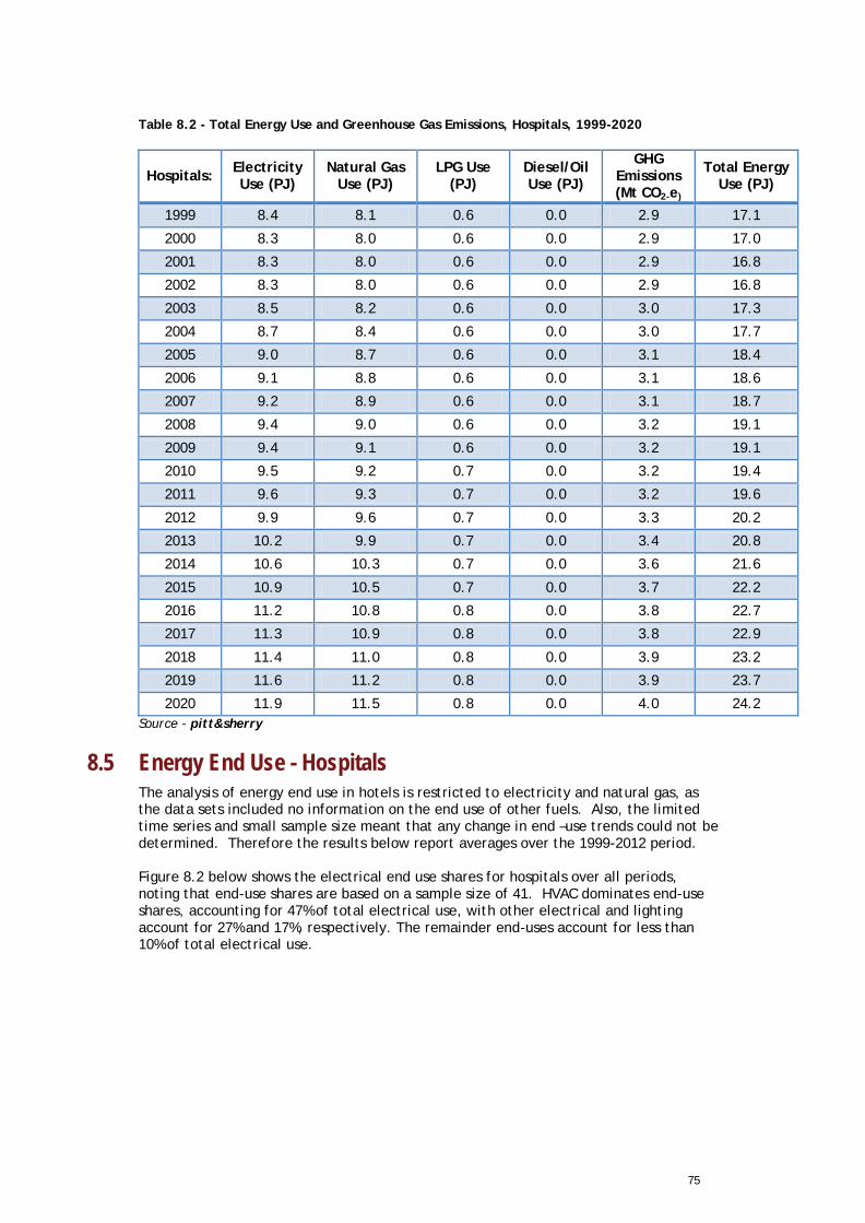
75

Table 8.2 - Total Energy Use and Greenhouse Gas Emissions, Hospitals, 1999-2020

Hospitals: Electricity Use (PJ)

Natural Gas Use (PJ)

LPG Use (PJ)

Diesel/Oil Use (PJ)

GHG Emissions (Mt CO2-e)

Total Energy Use (PJ)

1999 8.4 8.1 0.6 0.0 2.9 17.1

2000 8.3 8.0 0.6 0.0 2.9 17.0

2001 8.3 8.0 0.6 0.0 2.9 16.8

2002 8.3 8.0 0.6 0.0 2.9 16.8

2003 8.5 8.2 0.6 0.0 3.0 17.3

2004 8.7 8.4 0.6 0.0 3.0 17.7

2005 9.0 8.7 0.6 0.0 3.1 18.4

2006 9.1 8.8 0.6 0.0 3.1 18.6

2007 9.2 8.9 0.6 0.0 3.1 18.7

2008 9.4 9.0 0.6 0.0 3.2 19.1

2009 9.4 9.1 0.6 0.0 3.2 19.1

2010 9.5 9.2 0.7 0.0 3.2 19.4

2011 9.6 9.3 0.7 0.0 3.2 19.6

2012 9.9 9.6 0.7 0.0 3.3 20.2

2013 10.2 9.9 0.7 0.0 3.4 20.8

2014 10.6 10.3 0.7 0.0 3.6 21.6

2015 10.9 10.5 0.7 0.0 3.7 22.2

2016 11.2 10.8 0.8 0.0 3.8 22.7

2017 11.3 10.9 0.8 0.0 3.8 22.9

2018 11.4 11.0 0.8 0.0 3.9 23.2

2019 11.6 11.2 0.8 0.0 3.9 23.7

2020 11.9 11.5 0.8 0.0 4.0 24.2 Source - pitt&sherry

8.5 Energy End Use - Hospitals The analysis of energy end use in hotels is restricted to electricity and natural gas, as the data sets included no information on the end use of other fuels. Also, the limited time series and small sample size meant that any change in end –use trends could not be determined. Therefore the results below report averages over the 1999-2012 period. Figure 8.2 below shows the electrical end use shares for hospitals over all periods, noting that end-use shares are based on a sample size of 41. HVAC dominates end-use shares, accounting for 47% of total electrical use, with other electrical and lighting account for 27% and 17%, respectively. The remainder end-uses account for less than 10% of total electrical use.

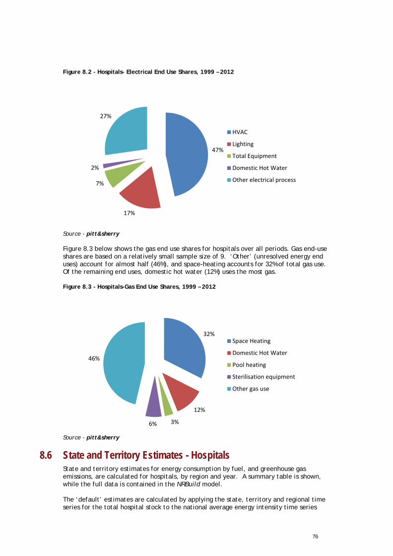
76

Figure 8.2 - Hospitals- Electrical End Use Shares, 1999 – 2012

. Source - pitt&sherry Figure 8.3 below shows the gas end use shares for hospitals over all periods. Gas end-use shares are based on a relatively small sample size of 9. ‘Other’ (unresolved energy end uses) account for almost half (46%), and space-heating accounts for 32% of total gas use. Of the remaining end uses, domestic hot water (12%) uses the most gas. Figure 8.3 - Hospitals-Gas End Use Shares, 1999 – 2012

. Source - pitt&sherry

8.6 State and Territory Estimates - Hospitals State and territory estimates for energy consumption by fuel, and greenhouse gas emissions, are calculated for hospitals, by region and year. A summary table is shown, while the full data is contained in the NRBuild model. The ‘default’ estimates are calculated by applying the state, territory and regional time series for the total hospital stock to the national average energy intensity time series

47%

17%

7%

2%

27%

HVAC

Lighting

Total Equipment

Domestic Hot Water

Other electrical process

32%

12%

3% 6%

46%

Space Heating

Domestic Hot Water

Pool heating

Sterilisation equipment

Other gas use

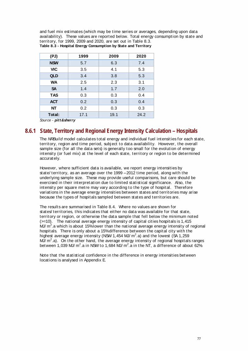
77

and fuel mix estimates (which may be time series or averages, depending upon data availability). These values are reported below. Total energy consumption by state and territory, for 1999, 2009 and 2020, are set out in Table 8.3. Table 8.3 - Hospital Energy Consumption by State and Territory

(PJ) 1999 2009 2020

NSW 5.7 6.3 7.4

VIC 3.5 4.1 5.3

QLD 3.4 3.8 5.3

WA 2.5 2.3 3.1

SA 1.4 1.7 2.0

TAS 0.3 0.3 0.4

ACT 0.2 0.3 0.4

NT 0.2 0.3 0.3

Total: 17.1 19.1 24.2 Source - pitt&sherry

8.6.1 State, Territory and Regional Energy Intensity Calculation – Hospitals The NRBuild model calculates total energy and individual fuel intensities for each state, territory, region and time period, subject to data availability. However, the overall sample size (for all the data sets) is generally too small for the evolution of energy intensity (or fuel mix) at the level of each state, territory or region to be determined accurately. However, where sufficient data is available, we report energy intensities by state/territory, as an average over the 1999 – 2012 time period, along with the underlying sample size. These may provide useful comparisons, but care should be exercised in their interpretation due to limited statistical significance. Also, the intensity per square metre may vary according to the type of hospital. Therefore variations in the average energy intensities between states and territories may arise because the types of hospitals sampled between states and territories are. The results are summarised in Table 8.4. Where no values are shown for states/territories, this indicates that either no data was available for that state, territory or region, or otherwise the data sample that fell below the minimum noted (>=10). The national average energy intensity of capital cities hospitals is 1,415 MJ/m2.a which is about 15% lower than the national average energy intensity of regional hospitals. There is only about a 15% difference between the capital city with the highest average energy intensity (NSW 1,454 MJ/m2.a) and the lowest (SA 1,259 MJ/m2.a). On the other hand, the average energy intensity of regional hospitals ranges between 1,039 MJ/m2.a in NSW to 1,684 MJ/m2.a in the NT, a difference of about 62%. Note that the statistical confidence in the difference in energy intensities between locations is analysed in Appendix E.

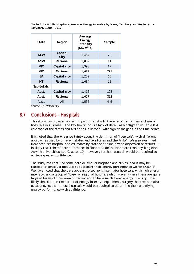
78

Table 8.4 - Public Hospitals, Average Energy Intensity by State, Territory and Region (n >= 10/year), 1999 – 2012

State Region

Average Energy

Intensity (MJ/m2.a)

Sample

NSW Capital City 1,454 28

NSW Regional 1,039 21

VIC Capital city 1,393 67

VIC Regional 1,677 271

SA Capital city 1,259 10

NT Regional 1,684 18

Sub-totals: Aust. Capital city 1,415 123

Aust. Regional 1,657 322

Aust. All 1,536 445 Source - pitt&sherry

8.7 Conclusions - Hospitals This study has provided a starting point insight into the energy performance of major hospitals in Australia. The key limitation is a lack of data. As highlighted in Table 8.4, coverage of the states and territories is uneven, with significant gaps in the time series. It is noted that there is uncertainty about the definition of ‘hospitals’, with different approaches used by different states and territories and the AIHW. We also examined floor area per hospital bed estimates by state and found a wide dispersion of results. It is likely that this reflects differences in floor area definitions more than anything else. As with universities (see Chapter 10), however, further research would be required to achieve greater confidence. The study has captured some data on smaller hospitals and clinics, and it may be feasible to construct modules to represent their energy performance within NRBuild. We have noted that the data appears to segment into major hospitals, with high energy intensity, and a group of ‘base’ or regional hospitals which – even where these are quite large in terms of floor area or beds – tend to have much lower energy intensity. It is likely that data on the extent of energy intensive equipment, surgery theatres and also occupancy levels in these hospitals would be required to determine their underlying energy performance with confidence.

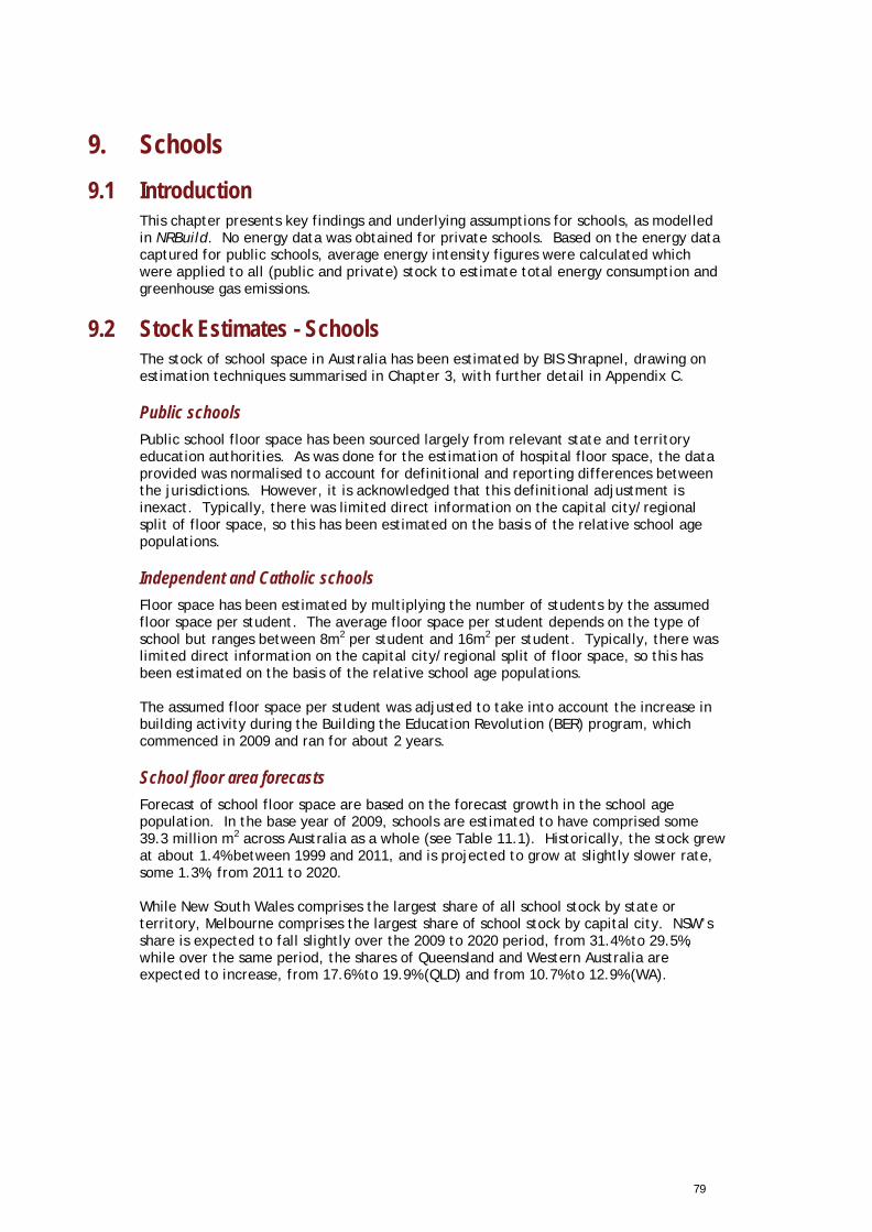
79

9. Schools 9.1 Introduction

This chapter presents key findings and underlying assumptions for schools, as modelled in NRBuild. No energy data was obtained for private schools. Based on the energy data captured for public schools, average energy intensity figures were calculated which were applied to all (public and private) stock to estimate total energy consumption and greenhouse gas emissions.

9.2 Stock Estimates - Schools The stock of school space in Australia has been estimated by BIS Shrapnel, drawing on estimation techniques summarised in Chapter 3, with further detail in Appendix C.

Public schools Public school floor space has been sourced largely from relevant state and territory education authorities. As was done for the estimation of hospital floor space, the data provided was normalised to account for definitional and reporting differences between the jurisdictions. However, it is acknowledged that this definitional adjustment is inexact. Typically, there was limited direct information on the capital city/regional split of floor space, so this has been estimated on the basis of the relative school age populations.

Independent and Catholic schools Floor space has been estimated by multiplying the number of students by the assumed floor space per student. The average floor space per student depends on the type of school but ranges between 8m2 per student and 16m2 per student. Typically, there was limited direct information on the capital city/regional split of floor space, so this has been estimated on the basis of the relative school age populations. The assumed floor space per student was adjusted to take into account the increase in building activity during the Building the Education Revolution (BER) program, which commenced in 2009 and ran for about 2 years.

School floor area forecasts Forecast of school floor space are based on the forecast growth in the school age population. In the base year of 2009, schools are estimated to have comprised some 39.3 million m2 across Australia as a whole (see Table 11.1). Historically, the stock grew at about 1.4% between 1999 and 2011, and is projected to grow at slightly slower rate, some 1.3%, from 2011 to 2020. While New South Wales comprises the largest share of all school stock by state or territory, Melbourne comprises the largest share of school stock by capital city. NSW’s share is expected to fall slightly over the 2009 to 2020 period, from 31.4% to 29.5%, while over the same period, the shares of Queensland and Western Australia are expected to increase, from 17.6% to 19.9% (QLD) and from 10.7% to 12.9% (WA).

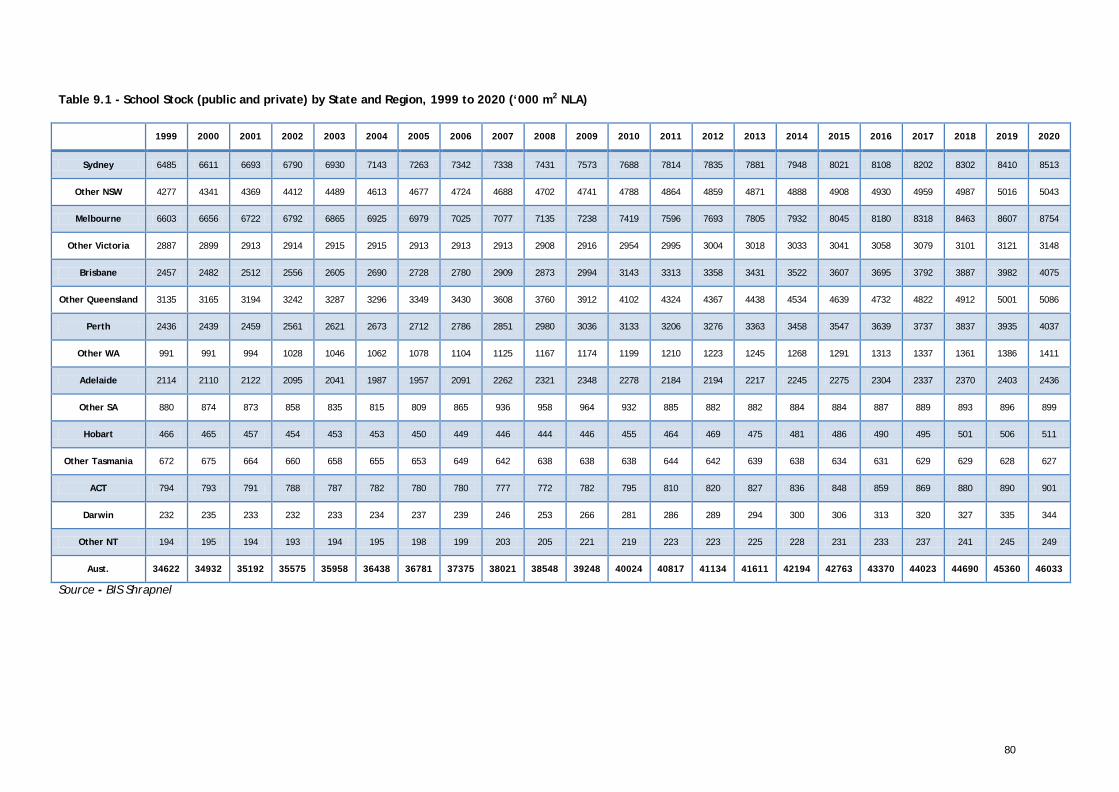
80

Table 9.1 - School Stock (public and private) by State and Region, 1999 to 2020 (‘000 m2 NLA)

1999 2000 2001 2002 2003 2004 2005 2006 2007 2008 2009 2010 2011 2012 2013 2014 2015 2016 2017 2018 2019 2020

Sydney 6485 6611 6693 6790 6930 7143 7263 7342 7338 7431 7573 7688 7814 7835 7881 7948 8021 8108 8202 8302 8410 8513

Other NSW 4277 4341 4369 4412 4489 4613 4677 4724 4688 4702 4741 4788 4864 4859 4871 4888 4908 4930 4959 4987 5016 5043

Melbourne 6603 6656 6722 6792 6865 6925 6979 7025 7077 7135 7238 7419 7596 7693 7805 7932 8045 8180 8318 8463 8607 8754

Other Victoria 2887 2899 2913 2914 2915 2915 2913 2913 2913 2908 2916 2954 2995 3004 3018 3033 3041 3058 3079 3101 3121 3148

Brisbane 2457 2482 2512 2556 2605 2690 2728 2780 2909 2873 2994 3143 3313 3358 3431 3522 3607 3695 3792 3887 3982 4075

Other Queensland 3135 3165 3194 3242 3287 3296 3349 3430 3608 3760 3912 4102 4324 4367 4438 4534 4639 4732 4822 4912 5001 5086

Perth 2436 2439 2459 2561 2621 2673 2712 2786 2851 2980 3036 3133 3206 3276 3363 3458 3547 3639 3737 3837 3935 4037

Other WA 991 991 994 1028 1046 1062 1078 1104 1125 1167 1174 1199 1210 1223 1245 1268 1291 1313 1337 1361 1386 1411

Adelaide 2114 2110 2122 2095 2041 1987 1957 2091 2262 2321 2348 2278 2184 2194 2217 2245 2275 2304 2337 2370 2403 2436

Other SA 880 874 873 858 835 815 809 865 936 958 964 932 885 882 882 884 884 887 889 893 896 899

Hobart 466 465 457 454 453 453 450 449 446 444 446 455 464 469 475 481 486 490 495 501 506 511

Other Tasmania 672 675 664 660 658 655 653 649 642 638 638 638 644 642 639 638 634 631 629 629 628 627

ACT 794 793 791 788 787 782 780 780 777 772 782 795 810 820 827 836 848 859 869 880 890 901

Darwin 232 235 233 232 233 234 237 239 246 253 266 281 286 289 294 300 306 313 320 327 335 344

Other NT 194 195 194 193 194 195 198 199 203 205 221 219 223 223 225 228 231 233 237 241 245 249

Aust. 34622 34932 35192 35575 35958 36438 36781 37375 38021 38548 39248 40024 40817 41134 41611 42194 42763 43370 44023 44690 45360 46033

Source - BIS Shrapnel

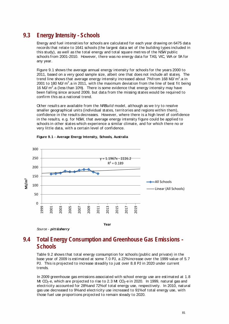
81

9.3 Energy Intensity - Schools Energy and fuel intensities for schools are calculated for each year drawing on 6475 data records that relate to 1641 schools (the largest data set of the building types included in this study), as well as the total energy and total square metres of the NSW public schools from 2001-2010. However, there was no energy data for TAS, VIC, WA or SA for any year. Figure 9.1 shows the average annual energy intensity for schools for the years 2000 to 2011, based on a very good sample size, albeit one that does not include all states. The trend line shows that average energy intensity increased about 7% from 168 MJ/m2.a in 2001 to 180 MJ/m2.a in 2011, with the maximum deviation from the line of best fit being 16 MJ/m2.a (less than 10%). There is some evidence that energy intensity may have been falling since around 2009, but data from the missing states would be required to confirm this as a national trend. Other results are available from the NRBuild model, although as we try to resolve smaller geographical units (individual states, territories and regions within them), confidence in the results decreases. However, where there is a high level of confidence in the results, e.g. for NSW, that average energy intensity figure could be applied to schools in other states which experience a similar climate, and for which there no or very little data, with a certain level of confidence. Figure 9.1 - Average Energy Intensity, Schools, Australia

.

Source - pitt&sherry

9.4 Total Energy Consumption and Greenhouse Gas Emissions - Schools Table 9.2 shows that total energy consumption for schools (public and private) in the base year of 2009 is estimated at some 7.0 PJ, a 22% increase over the 1999 value of 5.7 PJ. This is projected to increase steadily to just over 8.8 PJ in 2020 under current trends. In 2009 greenhouse gas emissions associated with school energy use are estimated at 1.8 Mt CO2-e, which are projected to rise to 2.3 Mt CO2-e in 2020. In 1999, natural gas and electricity accounted for 28% and 72% of total energy use, respectively. In 2010, natural gas use decreased to 9% and electricity use increased to 91% of total energy use, with those fuel use proportions projected to remain steady to 2020.

y = 1.1967x - 2226.2 R² = 0.189

0

50

100

150

200

250

300

1999

2001

2003

2005

2007

2009

2011

2013

2015

2017

2019

MJ/

m2

Year

All Schools

Linear (All Schools)

82

Table 9.2 - Total Energy Consumption and Greenhouse Gas Emissions, Schools, 1999-2020

Schools: Electricity Use (PJ)

Natural Gas Use (PJ)

LPG Use (PJ)

Diesel/Oil Use (PJ)

GHG Emissions (Mt CO2-e)

Total Energy Use (PJ)

1999 4.1 1.6 0.0 0.0 1.3 5.7

2000 4.2 1.6 0.0 0.0 1.3 5.8

2001 4.3 1.6 0.0 0.0 1.4 5.9

2002 4.3 1.7 0.0 0.0 1.4 6.0

2003 4.3 1.9 0.0 0.0 1.4 6.1

2004 4.6 1.7 0.0 0.0 1.4 6.3

2005 4.7 1.7 0.0 0.0 1.5 6.4

2006 5.0 1.5 0.0 0.0 1.5 6.5

2007 5.4 1.2 0.0 0.0 1.6 6.7

2008 5.9 0.9 0.0 0.0 1.7 6.8

2009 6.1 0.9 0.0 0.0 1.8 7.0

2010 6.4 0.7 0.0 0.0 1.9 7.2

2011 6.7 0.7 0.0 0.0 1.9 7.4

2012 6.8 0.7 0.0 0.0 2.0 7.5

2013 6.9 0.7 0.0 0.0 2.0 7.6

2014 7.0 0.7 0.0 0.0 2.0 7.8

2015 7.2 0.8 0.0 0.0 2.1 7.9

2016 7.3 0.8 0.0 0.0 2.1 8.1

2017 7.5 0.8 0.0 0.0 2.2 8.3

2018 7.6 0.8 0.0 0.0 2.2 8.4

2019 7.8 0.8 0.0 0.0 2.3 8.6

2020 8.0 0.8 0.0 0.0 2.3 8.8 Source - pitt&sherry

9.5 Energy End Use - Schools Due to limited data, the analysis of energy end use in schools is restricted to the ACT and to electricity and natural gas only. Furthermore, because of that limited data sample, it was not possible to construct significant time series trends for energy end use, and therefore the data presented represent averages over the 1999 – 2012 period.

Figures 9.2 and 9.3 below shows the average electricity and average gas end-use shares for ACT schools, which are based on a total sample of 334 data points. Lighting and equipment dominate the electrical end-use shares, accounting for 40% and 30% respectively on average. HVAC accounts for a significant 27% of electrical energy use on average, while domestic hot water makes up 4% of the total school electricity energy use on average. HVAC also accounts for the overwhelming majority (92%) of gas end-use shares with domestic hot water making up the remaining 8%.

It is expected that energy end use shares in some other states/territories would quite different to those indicated for the ACT. A significant proportion of ACT schools’ energy is used for space-conditioning, most of which is for heating (gas). On the other hand, in the NT there is little or no heating needed but a significant cooling requirement which relies on electricity.

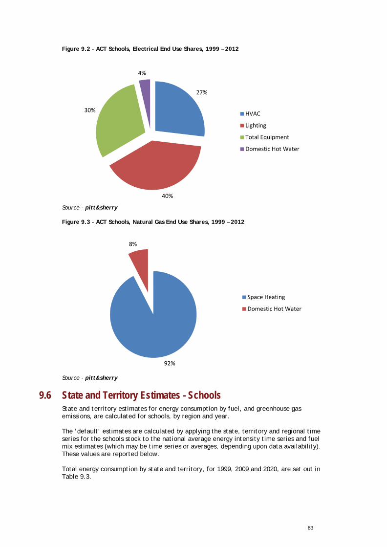
83

Figure 9.2 - ACT Schools, Electrical End Use Shares, 1999 – 2012

. Source - pitt&sherry

Figure 9.3 - ACT Schools, Natural Gas End Use Shares, 1999 – 2012

. Source - pitt&sherry

9.6 State and Territory Estimates - Schools State and territory estimates for energy consumption by fuel, and greenhouse gas emissions, are calculated for schools, by region and year. The ‘default’ estimates are calculated by applying the state, territory and regional time series for the schools stock to the national average energy intensity time series and fuel mix estimates (which may be time series or averages, depending upon data availability). These values are reported below.

Total energy consumption by state and territory, for 1999, 2009 and 2020, are set out in Table 9.3.

27%

40%

30%

4%

HVAC

Lighting

Total Equipment

Domestic Hot Water

92%

8%

Space Heating

Domestic Hot Water

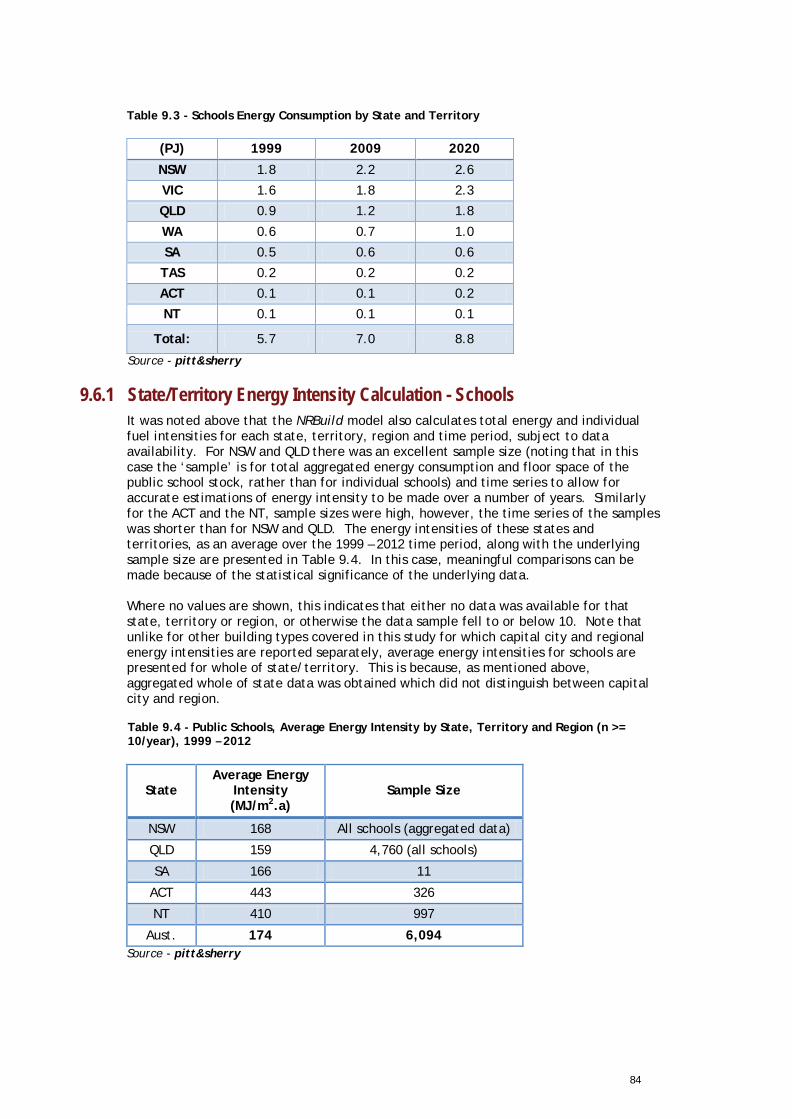
84

Table 9.3 - Schools Energy Consumption by State and Territory

(PJ) 1999 2009 2020

NSW 1.8 2.2 2.6

VIC 1.6 1.8 2.3

QLD 0.9 1.2 1.8

WA 0.6 0.7 1.0

SA 0.5 0.6 0.6

TAS 0.2 0.2 0.2

ACT 0.1 0.1 0.2

NT 0.1 0.1 0.1

Total: 5.7 7.0 8.8

Source - pitt&sherry

9.6.1 State/Territory Energy Intensity Calculation - Schools It was noted above that the NRBuild model also calculates total energy and individual fuel intensities for each state, territory, region and time period, subject to data availability. For NSW and QLD there was an excellent sample size (noting that in this case the ‘sample’ is for total aggregated energy consumption and floor space of the public school stock, rather than for individual schools) and time series to allow for accurate estimations of energy intensity to be made over a number of years. Similarly for the ACT and the NT, sample sizes were high, however, the time series of the samples was shorter than for NSW and QLD. The energy intensities of these states and territories, as an average over the 1999 – 2012 time period, along with the underlying sample size are presented in Table 9.4. In this case, meaningful comparisons can be made because of the statistical significance of the underlying data. Where no values are shown, this indicates that either no data was available for that state, territory or region, or otherwise the data sample fell to or below 10. Note that unlike for other building types covered in this study for which capital city and regional energy intensities are reported separately, average energy intensities for schools are presented for whole of state/territory. This is because, as mentioned above, aggregated whole of state data was obtained which did not distinguish between capital city and region.

Table 9.4 - Public Schools, Average Energy Intensity by State, Territory and Region (n >= 10/year), 1999 – 2012

State Average Energy

Intensity (MJ/m2.a)

Sample Size

NSW 168 All schools (aggregated data)

QLD 159 4,760 (all schools)

SA 166 11

ACT 443 326

NT 410 997

Aust. 174 6,094 Source - pitt&sherry

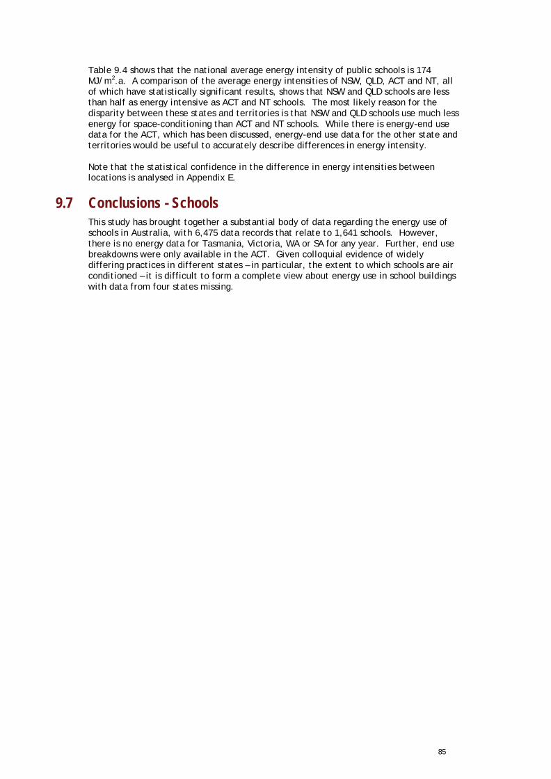
85

Table 9.4 shows that the national average energy intensity of public schools is 174 MJ/m2.a. A comparison of the average energy intensities of NSW, QLD, ACT and NT, all of which have statistically significant results, shows that NSW and QLD schools are less than half as energy intensive as ACT and NT schools. The most likely reason for the disparity between these states and territories is that NSW and QLD schools use much less energy for space-conditioning than ACT and NT schools. While there is energy-end use data for the ACT, which has been discussed, energy-end use data for the other state and territories would be useful to accurately describe differences in energy intensity. Note that the statistical confidence in the difference in energy intensities between locations is analysed in Appendix E.

9.7 Conclusions - Schools This study has brought together a substantial body of data regarding the energy use of schools in Australia, with 6,475 data records that relate to 1,641 schools. However, there is no energy data for Tasmania, Victoria, WA or SA for any year. Further, end use breakdowns were only available in the ACT. Given colloquial evidence of widely differing practices in different states – in particular, the extent to which schools are air conditioned – it is difficult to form a complete view about energy use in school buildings with data from four states missing.

86

10. Tertiary Education Buildings 10.1 Introduction

This section examines the energy consumption of tertiary education buildings in Australia. For the most part, the analysis deals with ‘precinct’ level information for Vocational Education and Training (VET) campuses (also known as TAFEs in some states) and university campuses. Depending upon the data source, individual buildings are not always resolved in reporting of total energy consumption and floor area. Some data on individual buildings within campuses is captured in the NRBuild model, although this data is generally treated as confidential. We note that precinct level data fails to distinguish between functionally diverse building types, from lecture theatres to physics laboratories, although the energy intensity of these building types is likely to vary greatly. Further, the energy data sources compiled for this study do not resolve the intensity of use of buildings, such as annual hours of use/operation, although this is likely to vary considerably between buildings, tertiary institutions and possibly states and territories.

10.2 Stock Estimates - Tertiary Education A stock model for tertiary education floor area was constructed by BIS Shrapnel, drawing on a wide range of data sources. As with most of the stock estimates, these are based on a ‘net lettable area’ equivalent concept, although there is significant uncertainty about the conceptual basis used in underlying data sources. A commonly used metric in universities is ‘Usable Floor Area’ (UFA), which means areas “directly used for Teaching and Research or support purposes”. 29 However a recent presentation to the Tertiary Education Facilities Management Association (TEFMA) Space Management Workshop, noted that eight tertiary institutions surveyed “…did not define or interpret their data codes in the same way or undertake benchmark reporting in the same way”, and that the results “varied so much that it wouldn’t be possible to use them accurately to complete the annual TEFMA benchmark survey…”.30 Examples of inconsistent reporting included the treatment of canteens, refectories, childcare facilities, circulation spaces, corridors and foyers, noting that many of these spaces may sometimes be used as ‘informal learning spaces’ in addition to their primary functions.

VET Public VET floor space is calculated using data provided by educational authorities for states and territories where available. A proxy based on student numbers is used where actual floor space data is not available, and for private VET providers. The National Centre for Vocational Education Research provides data on VET student numbers. The floor space for VET is estimated using the number of students and an average of the floor space per student of 3-6m2 per student. VET space forecasts are based in large part on analysis of the VET participation of the population by 5 year age group and forecast demographic trends.

29 S. Jones and J. Schumann, TEFMA Space Planning Guidelines and Go8 Data Dictionary, March 2011, accessed online at http://leishman-associates.com.au/tefmaspace2011/downloads/IntroductiontoSpaceDefinitionsWorkshop_000.pdf on 3 May 2012. 30 ibid.

87

Table 10.1 - Stock Estimates, TAFE/VET Floor Area, 1999 – 2020, ‘000m2

1999 2000 2001 2002 2003 2004 2005 2006 2007 2008 2009 2010 2011 2012 2013 2014 2015 2016 2017 2018 2019 2020

Sydney 1,071 1,077 1,063 1,051 1,051 1,052 1,032 1,092 1,063 1,063 1,058 1,061 1,066 1,071 1,077 1,084 1,090 1,096 1,102 1,108 1,114 1,120

Other NSW 985 989 979 967 967 972 955 1,013 973 954 950 952 957 961 966 972 977 983 988 994 999 1,004

Melbourne 1,143 1,143 1,157 1,174 1,189 1,180 1,150 1,150 1,167 1,189 1,240 1,290 1,300 1,310 1,320 1,334 1,345 1,357 1,369 1,381 1,394 1,406

Other Victoria 795 798 808 819 835 818 803 803 797 812 816 828 835 841 848 856 864 871 879 887 895 903

Brisbane 482 493 495 498 506 499 499 498 503 506 513 522 526 531 537 546 555 564 572 580 589 597

Other Queensland 694 710 712 732 734 733 739 737 734 726 735 748 754 761 771 783 796 808 820 832 844 856

Perth 352 361 378 370 371 366 372 360 359 371 397 423 428 434 442 451 459 466 474 482 489 497

Other WA 125 128 133 130 132 134 136 137 140 148 170 173 175 177 180 184 187 190 193 197 200 203

Adelaide 381 383 387 396 406 422 435 431 426 425 416 406 407 407 407 410 412 413 415 417 419 421

Other SA 145 145 146 147 149 148 152 150 149 149 149 152 153 152 153 154 154 155 156 156 157 158

Hobart 52 52 52 54 57 59 63 67 70 71 73 74 74 74 73 73 73 73 73 72 72 72

Other Tasmania 81 83 85 89 94 99 104 108 112 114 120 123 123 123 122 122 122 122 121 121 120 120

ACT 82 83 85 86 88 93 95 97 101 103 107 109 110 110 111 112 112 113 113 114 115 116

Darwin 15 15 16 15 15 15 16 16 16 17 19 20 20 20 21 21 22 22 22 23 23 23

Other NT 33 33 33 33 33 33 33 33 38 38 39 36 37 37 38 39 39 40 40 41 42 42

Aust. 6,435 6,494 6,530 6,562 6,628 6,623 6,582 6,691 6,648 6,686 6,802 6,917 6,964 7,009 7,066 7,142 7,208 7,272 7,338 7,403 7,470 7,537

Source - BIS Shrapnel

88

Table 10.2 - Stock Estimates, University Floor Area, 1999 – 2020, ‘000m2

1999 2000 2001 2002 2003 2004 2005 2006 2007 2008 2009 2010 2011 2012 2013 2014 2015 2016 2017 2018 2019 2020

Sydney 1,157 1,157 1,300 1,385 1,436 1,416 1,404 1,465 1,548 1,664 1,858 1,970 2,077 2,128 2,178 2,231 2,284 2,338 2,394 2,451 2,510 2,570

Other NSW 486 486 546 612 664 675 690 702 730 765 816 860 895 916 938 959 982 1,005 1,028 1,052 1,076 1,101

Melbourne 1,171 1,171 1,316 1,404 1,469 1,524 1,535 1,595 1,720 1,835 1,998 2,110 2,222 2,275 2,329 2,383 2,440 2,497 2,556 2,616 2,678 2,741

Other Victoria 269 269 302 332 358 378 379 403 437 457 471 483 504 516 528 540 552 565 578 591 605 619

Brisbane 617 617 693 740 759 763 771 798 836 859 931 1,019 1,070 1,095 1,121 1,147 1,174 1,202 1,230 1,259 1,288 1,318

Other Queensland 348 348 391 411 422 471 555 571 518 506 569 587 616 632 647 662 678 694 711 728 746 764

Perth 548 548 616 654 716 734 760 790 811 868 968 1,036 1,086 1,112 1,139 1,166 1,194 1,223 1,252 1,282 1,313 1,344

Other WA 0 0 0 0 0 0 0 0 0 0 0 0 0 0 0 0 0 0 0 0 0 0

Adelaide 375 375 421 433 463 491 491 514 548 567 598 626 653 669 684 700 717 733 750 768 786 804

Other SA 1 1 1 1 1 1 1 1 3 4 4 3 0 0 0 0 0 0 0 0 0 0

Hobart 129 129 145 154 156 190 183 183 188 178 179 184 192 196 201 205 210 215 220 225 230 235

Other Tasmania 1 1 1 1 1 1 1 1 3 4 4 3 0 0 0 0 0 0 0 0 0 0

ACT 270 270 304 327 355 252 228 228 216 229 356 352 366 375 383 392 401 410 420 429 439 449

Darwin 189 189 212 231 210 139 100 100 82 76 84 78 82 83 85 87 89 91 93 96 98 100

Other NT 0 0 0 0 0 0 0 0 0 0 0 0 0 0 0 0 0 0 0 0 0 0

Aust. 5,561 5,561 6,247 6,686 7,011 7,034 7,099 7,353 7,640 8,011 8,837 9,312 9,763 9,997 10,233 10,474 10,721 10,974 11,233 11,498 11,769 12,047

Source - BIS Shrapnel

89

Universities Actual university floor space data is available for 17 universities, including most of the major universities on a GFA basis. This was adjusted to an NLA basis. Where floor space data is unavailable, floor space has been estimated using data on the number of internal full-time students, sourced from Department of Education, Employment and Workplace Relations and an estimated usable NLA per internal full-time student ratio of 14-15m2 per student. The backcast estimates have been derived using information on internal full time student numbers.

10.2.1 Stock Estimates - VET Table 10.1 provides the stock estimates for VET floor area by state, territory and region for the period 1999 to 2020. In the base year of 2009, it is estimated that there were almost 6.7 million m2 of VET building floor area in Australia, only 4% more than the 1999 estimate of around 6.4 million m2. 56% of the stock is located in capital cities.

Over the period 2009 to 2020, somewhat faster growth in floor area of 14% over the period is expected (reflecting an expectation of increasing participation and population). This would see total floor area reaching some 7.6 million m2 by 2020.

10.2.2 Stock Estimates - Universities Table 10.2 presents the stock estimates for university floor area. In 2009, we estimate there were around 8.8 million m2 of university floor area across Australia. In contrast to TAFE campuses, some 79% of the floor area is located in capital cities. Also in contrast to TAFEs, the floor area of universities grew very rapidly over the 1999 to 2009 period, by 59%, representing a cumulative annual growth rate of 4.7% on average. The projections for 2020 show continued and reasonably rapid growth, albeit at the more modest pace of 2.5% per year on average, to reach almost 12.4 million m2 by 2020.

10.3 Energy Intensity - Tertiary Education Buildings The analysis of energy and fuel intensity in tertiary buildings is based on 1277 data records, relating to 388 individual buildings. Over all periods, the data coverage includes more than 14 million m2 of floor area although, some of this floor area represents time series data for the same building. The VET data provides significant observations over the 2003 to 2010 period (total n=148), but is geographically restricted, relating mostly to WA, SA, NSW and Tas in that order, with no data on the other states. Data from the early part of this time series is dominated by one state, WA. The universities data set is larger (total n=1,238), provides significant results observations over the 2001 – 2011 period, and covers most regions except Perth and the NT.

10.3.1 Energy Intensity - VET Buildings Figure 10.1 shows that, on average, the trend in energy intensity in VET buildings over the period 2003 – 2010 has been quite flat at around 365 MJ/m2.a. A slightly declining trend may have been evident in the absence of the 2010 result which, due to the limited sample size in that year (n=41), is being dragged upwards by results from one climate zone, Adelaide. With additional data capture, particularly for the ‘missing’ states noted above, a more robust trend may be able to be established. The outlier result in 2010 also contributes to a very low ‘R2’ value, indicating a reasonable degree of ‘scattering’ of data points around the trend. However, we note that annual variability around the trend never exceeds 37 MJ/m2.a, or around 10% of the average value.

90

Figure 10.1 - Average Energy Intensity, VETs, Australia, 2003 – 2010

Source - pitt&sherry

10.3.2 Energy Intensity - University Buildings Figure 10.2 shows the trend over 2001 to 2011 in the national average energy intensity of university buildings in Australia. It shows a modest increase through time, rising from an estimated 780 MJ/m2.a in 1999 to around 869 MJ/m2.a by the base year of 2009. The minimum sample that informs this trend in each year is 49 data records. As with other regressions for average energy intensity, the R2 value is very low, and in this case there are significant outlier values (eg, 2008) that vary by around 25% from the trend line. Figure 10.2 - Average Energy Intensity, Universities, Australia, 2001 – 2011

. Source - pitt&sherry An investigation of the causes of the apparent instability in the average energy intensity of university buildings through time has revealed that the primary cause is that the mix of different building sub-types within the data sample changes from year to year. The energy data includes the sub-type ‘laboratories’ within the overall ‘universities’ building type. Individual laboratories vary very widely in their energy intensity (in our data set, between 10 MJ/m2.a to over 7,500 MJ/m2.a), depending largely on their type/purpose (the low values are often ‘agricultural research stations’, for example). As the energy intensity data captured for this study is essentially a random sample in each year, the mix of building sub-types within any given sample can vary, leading to significant changes in the measured average energy intensity. This indicates that the model should resolve these building subtypes separately, with separate stock and energy intensity observations. For further statistical analysis, refer to Appendix E.

R² = 0.0002 050

100150200250300350400450

1999

2001

2003

2005

2007

2009

2011

2013

2015

2017

2019

MJ/

m2 .a

Year

n>=9

Linear(n>=9)

R² = 0.041 0

200

400

600

800

1,000

1,200

1999

2001

2003

2005

2007

2009

2011

2013

2015

2017

2019

MJ/

m2 .a

Year

n>=49

Linear (n>=49)

91

10.4 Total Energy Consumption and Greenhouse Gas Emissions - Tertiary Education

10.4.1 VET Buildings Table 10.3 summarises total energy use by fuel and greenhouse gas emissions associated with VET buildings in Australia. Total energy consumption in the base year of 2009 was around 2.5 PJ, and indeed this figure has been largely static over the period from 1999. This reflects the slow growth in the stock of such buildings, together with the flat trend in energy intensity noted above. Total energy consumption is projected to rise slowly, reaching around 2.8 PJ in 2020. Greenhouse gas emissions are also largely static at around 0.6 Mt CO2-e. The average fuel mix in VET buildings is dominated by electricity, at around 81% (see Figure 10.3), with the majority of the balance accounted for by natural gas (17%) and minor use of LPG (2%). Table 10.3 - Total Energy Consumption and Greenhouse Gas Emissions, Vocational Education and Training (VET) Buildings, Australia, 1999 – 2020

Tertiary - VET:

Electricity Use (PJ)

Natural Gas Use (PJ) LPG Use (PJ) Diesel/Oil

Use (PJ)

GHG Emissions (Mt CO2-e)

Total Energy

Use (PJ)

1999 1.9 0.40 0.05 0.00 0.6 2.4

2000 1.9 0.4 0.0 0.0 0.6 2.4

2001 1.9 0.4 0.0 0.0 0.6 2.4

2002 2.0 0.4 0.0 0.0 0.6 2.4

2003 2.0 0.4 0.0 0.0 0.6 2.4

2004 2.0 0.4 0.0 0.0 0.6 2.4

2005 2.0 0.4 0.0 0.0 0.6 2.4

2006 2.0 0.4 0.1 0.0 0.6 2.5

2007 2.0 0.4 0.0 0.0 0.6 2.4

2008 2.0 0.4 0.1 0.0 0.6 2.5

2009 2.0 0.4 0.1 0.0 0.6 2.5

2010 2.1 0.4 0.1 0.0 0.6 2.5

2011 2.1 0.4 0.1 0.0 0.6 2.6

2012 2.1 0.4 0.1 0.0 0.6 2.6

2013 2.1 0.4 0.1 0.0 0.6 2.6

2014 2.1 0.4 0.1 0.0 0.6 2.6

2015 2.1 0.5 0.1 0.0 0.6 2.6

2016 2.2 0.5 0.1 0.0 0.6 2.7

2017 2.2 0.5 0.1 0.0 0.7 2.7

2018 2.2 0.5 0.1 0.0 0.7 2.7

2019 2.2 0.5 0.1 0.0 0.7 2.7

2020 2.2 0.5 0.1 0.0 0.7 2.8 Source - pitt&sherry

92

Figure 10.3 - VET Buildings– Fuel Shares, Australia 2010

. Source - pitt&sherry

10.4.2 Universities Table 10.4 shows that in the base year of 2009, estimated total energy use for university buildings was around 7.7 PJ, a substantial 79% increase over 1999. By 2020, total energy consumption is projected to increase by a further 50%, to reach around 11.6 PJ. Table 10.4 - Total Energy Consumption by Fuel and Greenhouse Gas Emissions, Universities, Australia, 1999 – 2020

Tertiary (University):

Electricity Use (PJ)

Natural Gas Use

(PJ)

LPG Use (PJ)

Diesel/Oil Use (PJ)

GHG Emissions (Mt CO2-e)

Total Energy Use (PJ)

1999 3.0 1.3 0.0 0.0 1.0 4.3

2000 3.0 1.3 0.0 0.0 1.0 4.4

2001 3.4 1.5 0.0 0.0 1.1 5.0

2002 3.7 1.7 0.0 0.0 1.2 5.4

2003 3.9 1.8 0.0 0.0 1.3 5.7

2004 4.0 1.8 0.0 0.0 1.3 5.8

2005 4.1 1.8 0.0 0.0 1.3 5.9

2006 4.2 1.9 0.0 0.0 1.3 6.2

2007 4.5 2.0 0.0 0.0 1.4 6.5

2008 4.7 2.1 0.0 0.0 1.5 6.9

2009 5.3 2.4 0.0 0.0 1.6 7.7

2010 5.6 2.5 0.1 0.0 1.7 8.2

2011 5.9 2.7 0.1 0.0 1.8 8.6

2012 6.1 2.7 0.1 0.0 1.9 8.9

2013 6.3 2.8 0.1 0.0 2.0 9.2

2014 6.6 2.9 0.1 0.0 2.0 9.6

2015 6.8 3.0 0.1 0.0 2.1 9.9

2016 7.0 3.1 0.1 0.0 2.2 10.2

2017 7.2 3.2 0.1 0.0 2.2 10.5

2018 7.5 3.3 0.1 0.0 2.3 10.9

2019 7.7 3.5 0.1 0.0 2.4 11.3

2020 8.0 3.6 0.1 0.0 2.5 11.6 Source - pitt&sherry

81%

17% 2%

ElectricityGasLPG

93

This growth reflects both the rapid expansion of university floor area historically, which is projected to continue albeit at a more moderate pace, along with rising energy intensity. We note there is uncertainty about both of these key drivers. University enrolments – particularly by overseas students – have declined in recent years, while significant efforts are being made by most campuses to improve their energy efficiency. In 2009 greenhouse gas emissions associated with energy use in university buildings are estimated at 1.6 Mt CO2-e, and are projected to rise to some 2.5 Mt CO2-e in 2020. The average fuel mix is expected to remain steady throughout the entire period at around 71% electricity and 28% natural gas, with minor use of LPG (see Figure 10.4). Figure 10.4 - University Buildings Fuel Shares, Australia, 2009

. Source - pitt&sherry

10.5 Energy End Use - Universities The data compiled for this study included a limited number of end-use breakdowns (n=96). This information was limited to electrical end use, and the values reported represent averages over the 1999 – 2012 time period. Figure 10.5 shows the average electricity end-use shares. Heating, ventilation and air conditioning (HVAC) dominates at around 50%, while lighting (18%), equipment (15%) and process energy use (e.g., in laboratories, 15%), account for the majority of the balance. Figure 10.5 - Universities- Electrical End Use Shares, Australia, 1999 – 2012

Source - pitt&sherry

71%

28%

1%

Electricity Natural Gas LPG

50%

18%

15%

2%

15%

HVAC

Lighting

Total Equipment

Domestic Hot Water

Other electrical process

94

10.6 States and Territory Estimates - Tertiary Education

10.6.1 Vocational Education and Training As noted in Section 12.3.1 above, the overall data sample for VET buildings available to this study was limited, with a total of 148 records used in the model. The sample is weighted towards WA and SA, with very limited for NSW and TAS and no data for the other states and territories. As a result, it is difficult to draw any conclusions about relative energy intensities between states, territories and regions. Nevertheless, the data suggests that capital city VET buildings are on average somewhat more energy intensive than those in regional areas, at around 470 MJ/m2.a as compared to around 370 MJ/m2.a for the latter. Tasmania appears to be much more energy intensive than other states, at over 800 MJ/m2.a, although this is based on a single campus accounting for around 10% of the estimated stock in that state. Table 10.3 provides an overview of the NRBuild estimates for total energy consumption by states and territories for VET buildings. Estimates are based on the national average energy intensities reported above as the default, distributed by state according the stock shares shown in Table 10.1. As with other building types, the NRBuild model allows the user to test alternative values for energy intensity, including by state. Estimate for greenhouse gas emissions and energy consumption by fuel for the intervening years and by region within states and territories are also available in the model. Table 10.5 - Vocational Education and Training Buildings, Total Energy Consumption by State, 1999, 2009, 2020

(PJ) 1999 2009 2020

NSW 0.8 0.7 0.8

VIC 0.7 0.8 0.8

QLD 0.4 0.5 0.5

WA 0.2 0.2 0.3

SA 0.2 0.2 0.2

TAS 0.0 0.1 0.1

ACT 0.0 0.0 0.0

NT 0.0 0.0 0.0

Total: 2.4 2.5 2.8 Source - pitt&sherry

10.6.2 Universities The data sample available to this study for universities was considerably larger than for VET buildings, thanks to excellent co-operation from a number of Australian universities, with 1,238 records in total. The sample covers all states, territories and regions except Perth and the Northern Territory. A data sample of at least 49 was available for each year between 2001 and 2011. Despite this, the data sample was not large enough to establish separate time series trends for energy intensity by state, territory and region. However, if we examine the average energy intensities over the whole period at that level of resolution, we note that capital city universities appear to be more than twice as energy intensive, on average, as those in regional areas, at over 860 MJ/m2.a (n=757) compared with around 420 MJ/m2.a (n=481) for the latter. Universities in Victoria appear to be the most energy intensive, at over 1,100 MJ/m2.a, although the sample is small (n=10), while the ACT also reports a similar value (n=13). Adelaide also reports an above average energy intensity of around 900 MJ/m2.a (n=111). Tasmania’s average energy intensity is below the national average, at around 700 MJ/m2.a in the capital (n=160) and less than 600 MJ/m2.a in regional areas (n=189).

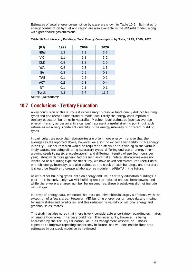
95

Estimates of total energy consumption by state are shown in Table 10.5. Estimates for energy consumption by fuel and region are also available in the NRBuild model, along with greenhouse gas emissions. Table 10.6 - University Buildings, Total Energy Consumption by State, 1999, 2009, 2020

(PJ) 1999 2009 2020

NSW 1.3 2.3 3.5

VIC 1.1 2.1 3.2

QLD 0.8 1.3 2.0

WA 0.4 0.8 1.3

SA 0.3 0.5 0.8

TAS 0.1 0.2 0.2

ACT 0.2 0.3 0.4

NT 0.1 0.1 0.1

Total: 4.3 7.7 11.6 Source - pitt&sherry

10.7 Conclusions - Tertiary Education A key conclusion of this study is it is necessary to resolve functionally distinct building types and end uses to understand or model accurately the energy consumption of tertiary education buildings in Australia. Precinct level estimates (such as average energy intensity across an entire campus) represent a useful starting point, but such estimates mask very significant diversity in the energy intensity of different building types. In particular, we note that laboratories are often more energy intensive that the average results reported above, however we also find extreme variability in this energy intensity. Further research would be required to attribute this finding to the various likely causes, including differing laboratory types, differing end-use of energy (from growing seeds to particle accelerators), and differing intensity of use (eg, hours per year), along with more generic factors such as climate. While laboratories were not identified as a building type for this study, we have nevertheless captured useful data on their energy intensity, and also estimated the stock of such buildings, and therefore it should be feasible to create a laboratories module in NRBuild in the future. As with other building types, data on energy end use in tertiary education buildings is poor. In this study, only two VET building records included end use breakdowns, and while there were are larger number for universities, these breakdowns did not include natural gas. In terms of energy data, we noted that data on universities is largely sufficient, with the exception of a few states. However, VET building energy performance data is missing for many states and territories, and this reduces the validity of national energy and greenhouse estimates. This study has also noted that there is very considerable uncertainty regarding estimates of ‘usable floor area’ in tertiary buildings. This uncertainty, however, is being addressed by the Tertiary Education Facilities Management Association. This is expected to improve reporting consistency in future, and will also enable floor area estimates in our stock model to be reviewed.

96

11. Public Buildings 11.1 Introduction

This chapter presents key findings and underlying assumptions for public buildings, law courts and correctional centres, as modelled in NRBuild. The scope of public buildings covered includes museums, galleries and libraries. As discussed below, however, there was only a limited data sample on each and therefore they have been modelled as a single ‘public buildings’ type. Law courts were modelled separately, and while stock estimates for correctional centres are presented, no usable energy intensity data on such centres was captured in this study and therefore this building type is not modelled.

11.2 Stock Estimates - Public Buildings Museums The museum floor space estimates are based on data from the Sydney Floor Space and Employment Survey, the Melbourne Census of Land Use and Employment Survey and the Perth Land Use and Employment Survey as well as data from individual museums where available. In addition, the DCCEE publishes information on the floorspace of Commonwealth operated museums, which was used. This method means that the floor space data for the main museums is included in the museum floor space estimates but that the floor space for a large number of smaller museums is excluded. The large number of different data sources also means that definitional issues are likely to significantly affect state comparisons of floor space.

Galleries The gallery floor space estimates have been compiled using a similar methodology to that for museums. The estimates are based on a combination of data from the Sydney Floor Space and Employment Survey, the Melbourne Census of Land Use and Employment Survey and the Perth Land Use and Employment Survey as well as data from individual museums where available, and data from the DCCEE for Commonwealth operated galleries. This method means that the floor space data for the main galleries is included in the museum floor space estimates but that the floor space for a large number of smaller galleries is excluded. As for museums, the large number of different data sources means that definitional issues are likely to affect state comparisons of floor space.

Libraries The floor space estimates for libraries are based on a number of different data sources. Where possible, information is sourced for the main national and state libraries on a site basis. ABS Cat 8561.0 includes information on the number of local government libraries and employment in local government libraries, which has been used to generate estimates for the floor area of local government libraries. The trend in library floor space is forecast to be flat.

Table 11.1 shows that public buildings (museums, galleries and libraries together) are estimated to have comprised some 1.8 million m2 NLA across Australia in the base year of 2009. There was limited information from which to develop historical public building stock estimates. The floor stock estimates have been adjusted for known developments, but otherwise the stock is assumed to be constant to 2020. New South Wales comprises the largest share (23.5%) of the public buildings by state.

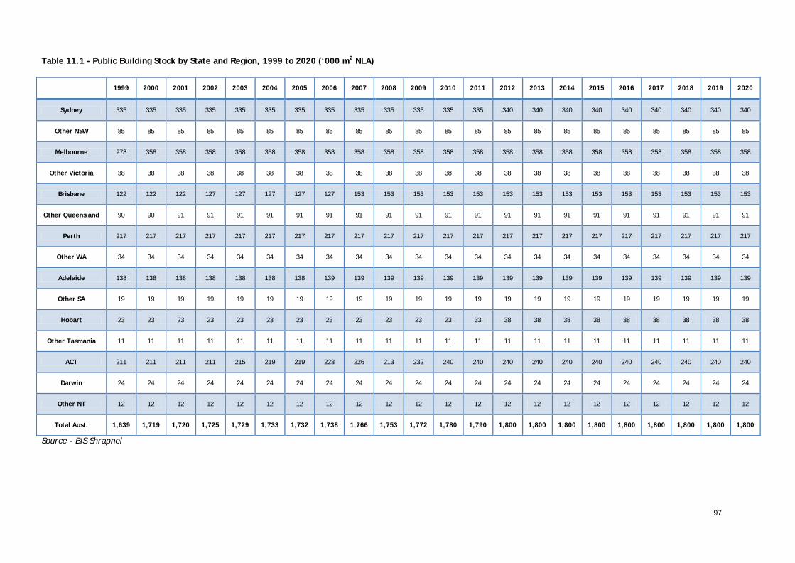
97

Table 11.1 - Public Building Stock by State and Region, 1999 to 2020 (‘000 m2 NLA)

1999 2000 2001 2002 2003 2004 2005 2006 2007 2008 2009 2010 2011 2012 2013 2014 2015 2016 2017 2018 2019 2020

Sydney 335 335 335 335 335 335 335 335 335 335 335 335 335 340 340 340 340 340 340 340 340 340

Other NSW 85 85 85 85 85 85 85 85 85 85 85 85 85 85 85 85 85 85 85 85 85 85

Melbourne 278 358 358 358 358 358 358 358 358 358 358 358 358 358 358 358 358 358 358 358 358 358

Other Victoria 38 38 38 38 38 38 38 38 38 38 38 38 38 38 38 38 38 38 38 38 38 38

Brisbane 122 122 122 127 127 127 127 127 153 153 153 153 153 153 153 153 153 153 153 153 153 153

Other Queensland 90 90 91 91 91 91 91 91 91 91 91 91 91 91 91 91 91 91 91 91 91 91

Perth 217 217 217 217 217 217 217 217 217 217 217 217 217 217 217 217 217 217 217 217 217 217

Other WA 34 34 34 34 34 34 34 34 34 34 34 34 34 34 34 34 34 34 34 34 34 34

Adelaide 138 138 138 138 138 138 138 139 139 139 139 139 139 139 139 139 139 139 139 139 139 139

Other SA 19 19 19 19 19 19 19 19 19 19 19 19 19 19 19 19 19 19 19 19 19 19

Hobart 23 23 23 23 23 23 23 23 23 23 23 23 33 38 38 38 38 38 38 38 38 38

Other Tasmania 11 11 11 11 11 11 11 11 11 11 11 11 11 11 11 11 11 11 11 11 11 11

ACT 211 211 211 211 215 219 219 223 226 213 232 240 240 240 240 240 240 240 240 240 240 240

Darwin 24 24 24 24 24 24 24 24 24 24 24 24 24 24 24 24 24 24 24 24 24 24

Other NT 12 12 12 12 12 12 12 12 12 12 12 12 12 12 12 12 12 12 12 12 12 12

Total Aust. 1,639 1,719 1,720 1,725 1,729 1,733 1,732 1,738 1,766 1,753 1,772 1,780 1,790 1,800 1,800 1,800 1,800 1,800 1,800 1,800 1,800 1,800

Source - BIS Shrapnel

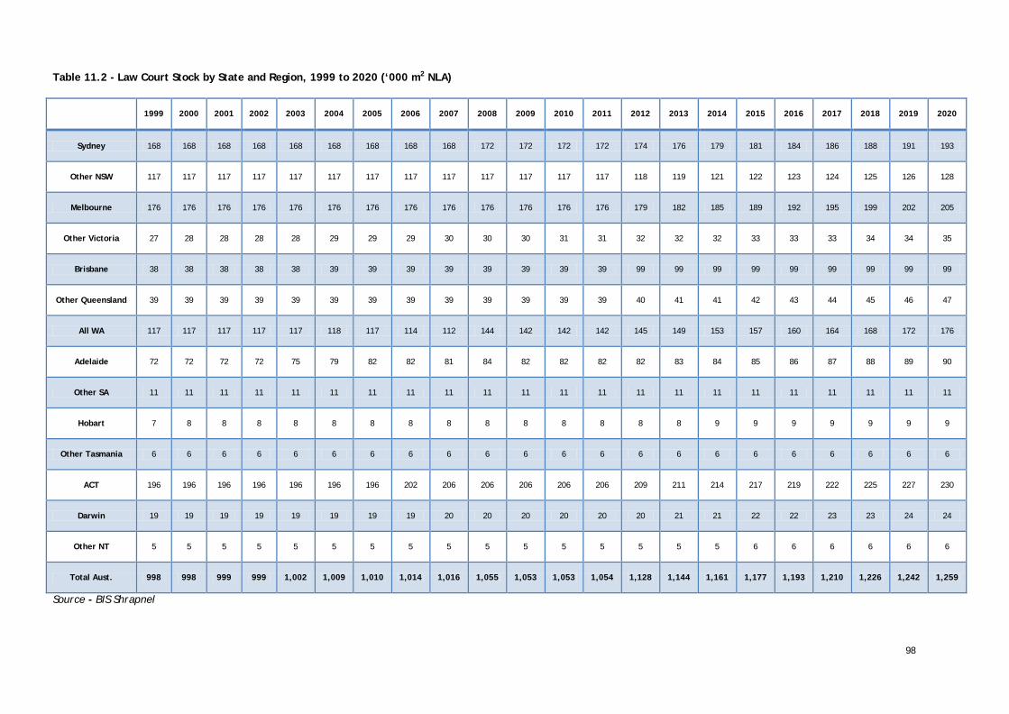
98

Table 11.2 - Law Court Stock by State and Region, 1999 to 2020 (‘000 m2 NLA)

1999 2000 2001 2002 2003 2004 2005 2006 2007 2008 2009 2010 2011 2012 2013 2014 2015 2016 2017 2018 2019 2020

Sydney 168 168 168 168 168 168 168 168 168 172 172 172 172 174 176 179 181 184 186 188 191 193

Other NSW 117 117 117 117 117 117 117 117 117 117 117 117 117 118 119 121 122 123 124 125 126 128

Melbourne 176 176 176 176 176 176 176 176 176 176 176 176 176 179 182 185 189 192 195 199 202 205

Other Victoria 27 28 28 28 28 29 29 29 30 30 30 31 31 32 32 32 33 33 33 34 34 35

Brisbane 38 38 38 38 38 39 39 39 39 39 39 39 39 99 99 99 99 99 99 99 99 99

Other Queensland 39 39 39 39 39 39 39 39 39 39 39 39 39 40 41 41 42 43 44 45 46 47

All WA 117 117 117 117 117 118 117 114 112 144 142 142 142 145 149 153 157 160 164 168 172 176

Adelaide 72 72 72 72 75 79 82 82 81 84 82 82 82 82 83 84 85 86 87 88 89 90

Other SA 11 11 11 11 11 11 11 11 11 11 11 11 11 11 11 11 11 11 11 11 11 11

Hobart 7 8 8 8 8 8 8 8 8 8 8 8 8 8 8 9 9 9 9 9 9 9

Other Tasmania 6 6 6 6 6 6 6 6 6 6 6 6 6 6 6 6 6 6 6 6 6 6

ACT 196 196 196 196 196 196 196 202 206 206 206 206 206 209 211 214 217 219 222 225 227 230

Darwin 19 19 19 19 19 19 19 19 20 20 20 20 20 20 21 21 22 22 23 23 24 24

Other NT 5 5 5 5 5 5 5 5 5 5 5 5 5 5 5 5 6 6 6 6 6 6

Total Aust. 998 998 999 999 1,002 1,009 1,010 1,014 1,016 1,055 1,053 1,053 1,054 1,128 1,144 1,161 1,177 1,193 1,210 1,226 1,242 1,259

Source - BIS Shrapnel

99

Table 11.3 - Correctional Centre Stock by State and Region, 1999 to 2020 (‘000 m2 NLA)

1999 2000 2001 2002 2003 2004 2005 2006 2007 2008 2009 2010 2011 2012 2013 2014 2015 2016 2017 2018 2019 2020

Sydney 172 179 190 196 197 200 214 221 225 231 240 239 247 250 253 257 261 264 268 272 275 279

Other NSW 102 106 113 116 116 118 126 131 132 136 140 139 143 145 146 148 150 151 153 154 156 158

Melbourne 77 83 88 93 99 100 98 99 110 114 118 123 127 128 131 133 135 137 139 141 143 145

Other Victoria 30 32 34 35 37 37 36 37 41 42 43 44 45 46 46 47 47 48 48 49 49 49

Brisbane 89 98 102 99 112 114 112 108 103 104 117 121 121 121 121 121 121 121 121 121 121 121

Other Queensland 110 120 125 121 137 135 134 129 125 125 141 146 158 174 174 174 174 174 174 174 174 174

Perth 78 83 87 97 108 109 111 112 112 112 114 114 118 120 124 127 130 134 137 141 144 148

Other WA 29 30 32 35 39 39 40 40 40 40 40 40 41 42 43 45 46 47 48 49 49 50

Adelaide 48 48 48 48 48 48 48 49 49 49 49 50 50 50 50 50 50 50 50 50 51 51

Other SA 58 58 58 58 58 59 59 60 60 60 60 61 61 61 61 61 61 61 61 61 62 62

Hobart 14 14 17 17 18 17 16 17 21 22 22 21 21 21 21 21 21 21 21 21 21 21

Other Tasmania 4 4 4 4 4 4 4 4 4 4 4 4 4 4 4 4 4 4 4 4 4 4

ACT 2 2 2 3 4 4 4 4 4 4 6 12 12 12 12 12 12 12 12 12 12 12

Darwin 12 14 14 14 14 14 14 14 15 15 16 19 19 20 20 27 27 27 34 34 34 34

Other NT 14 14 14 14 14 14 14 14 14 14 14 14 14 14 14 14 14 14 14 14 14 14

Total Aust. 837 882 927 949 1,003 1,009 1,030 1,036 1,054 1,072 1,122 1,148 1,181 1,209 1,221 1,242 1,254 1,265 1,284 1,296 1,309 1,322

Source - BIS Shrapnel

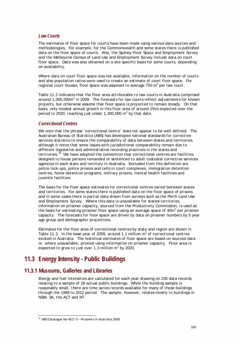
100

Law Courts The estimates of floor space for courts have been made using various data sources and methodologies. For example, for the Commonwealth and some states there is published data on the floor space of courts. Also, the Sydney Floor Space and Employment Survey and the Melbourne Census of Land Use and Employment Survey include data on court floor space. Data was also obtained on a site specific basis for some courts, depending on availability. Where data on court floor space was not available, information on the number of courts and also population ratios were used to create an estimate of court floor space. For regional court houses, floor space was assumed to average 750 m2 per law court. Table 11.2 indicates that the floor area attributable to law courts in Australia comprised around 1,000,000m2 in 2009. The forecasts for law courts reflect adjustments for known projects, but otherwise assume that floor space is projected to remain steady. On that basis, only modest annual growth in this floor area of around 2% is expected over the period to 2020, reaching just under 1,300,000 m2 by that date.

Correctional Centres We note that the phrase ‘correctional centre’ does not appear to be well defined. The Australian Bureau of Statistics (ABS) has developed national standards for corrective services statistics to ensure the comparability of data between states and territories, although it notes that some issues with jurisdictional comparability remain due to different legislative and administrative recording practices in the states and territories.31 We have adopted the convention that correctional centres are facilities designed to house persons remanded or sentenced to adult custodial corrective services agencies in each state and territory in Australia. Excluded from this definition are police lock-ups, police prisons and cells in court complexes, immigration detention centres, home detention programs, military prisons, mental health facilities and juvenile facilities. The basis for the floor space estimates for correctional centres varied between states and territories. For some states there is published data on the floor space of prisons and in some cases there is partial data drawn from surveys such as the Perth Land Use and Employment Survey. Where this data is unavailable for states/territories, information on prisoner capacity, sourced from the Productivity Commission, is used as the basis for estimating prisoner floor space using an average space of 40m2 per prisoner capacity. The forecasts for floor space are driven by data on prisoner numbers by 5 year age group and demographic projections. Estimates for the floor area of correctional centres by state and region are shown in Table 11.3. In the base year of 2009, around 1.1 million m2 of correctional centres existed in Australia. The historical estimates of floor space are based on sourced data or, where unavailable, proxied using information on prisoner capacity. Floor area is expected to grow to just over 1.3 million m2 by 2020.

11.3 Energy Intensity - Public Buildings

11.3.1 Museums, Galleries and Libraries Energy and fuel intensities are calculated for each year drawing on 235 data records relating to a sample of 28 actual public buildings. While the building sample is reasonably small, there are time series records available for many of these buildings through the 1999 to 2012 period. The sample, however, relates mostly to buildings in NSW, SA, the ACT and NT.

31 ABS Catalogue No 4517.0 – Prisoners in Australia 2008.

101

Figure 11.1 shows the average annual energy intensity for public buildings for the years 2001-2011, including linear regressions for the period back to 1999 and forward to 2020. The results shown are based on area-weighted average energy intensities for all regions in Australia, for each year in which the sample size (n) was at least 9. In the base year of 2009, the average energy intensity of public buildings in Australia is indicated to be just over 1,000 MJ/m2.a. It can be seen, however, that the trend is for a steady fall in the energy intensity of public buildings over time. The results show a reasonable R2 value of 0.623, with the maximum deviation from the trend being 50 MJ/m2.a. As the trend is based on a relatively small sample size, further data capture would be required to establish trends with greater confidence. The libraries within this data set appeared to be less energy intensive than the average public building, at just under 600 MJ/m2.a, although this result is based on a limited sample (n=14). Museums and galleries also appear to sub-divide into two sets: the larger, national institutions which have higher energy intensity, and smaller private galleries (and buildings such as aviation or motor museums) with quite low energy intensity. This suggests that ideally these building types would be modeled separately. Figure 11.1 - Public Building Average Energy Intensity, Australia, 2001 - 2010 (MJ/m2.a)

Source - pitt&sherry

11.3.2 Law Courts The sample of law courts examined for energy intensity calculations comprised two data types. First, some 341 records were compiled relating to identified court buildings across most states and territories (except regional areas of Vic, WA and SA) over the 1999 – 2011 period. In 2009, these data records covered a total of some 43,000 m2 of actual courts in Australia. Second, we were able to access some ‘agency level’ data that provided total fuel consumption and floor area for the entire Australia-wide portfolio of courts relating to the Family Court of Australia, Law Courts Ltd, the Administrative Appeal Tribunal and Fair Work Australia. This data is not broken down by state, but in total covered the energy consumption of an additional 45,000 m2 of actual court space in Australia in 2009. Thus the total data sample covered around 10% of court floor area in 2009 and a higher share in earlier years (18% in 2001, for example).

R² = 0.623

0

200

400

600

800

1,000

1,200

1999

2001

2003

2005

2007

2009

2011

2013

2015

2017

2019

MJ/

m2 .a

Year

n>=9

Linear (n>=9)

Total n value, all periods: 227

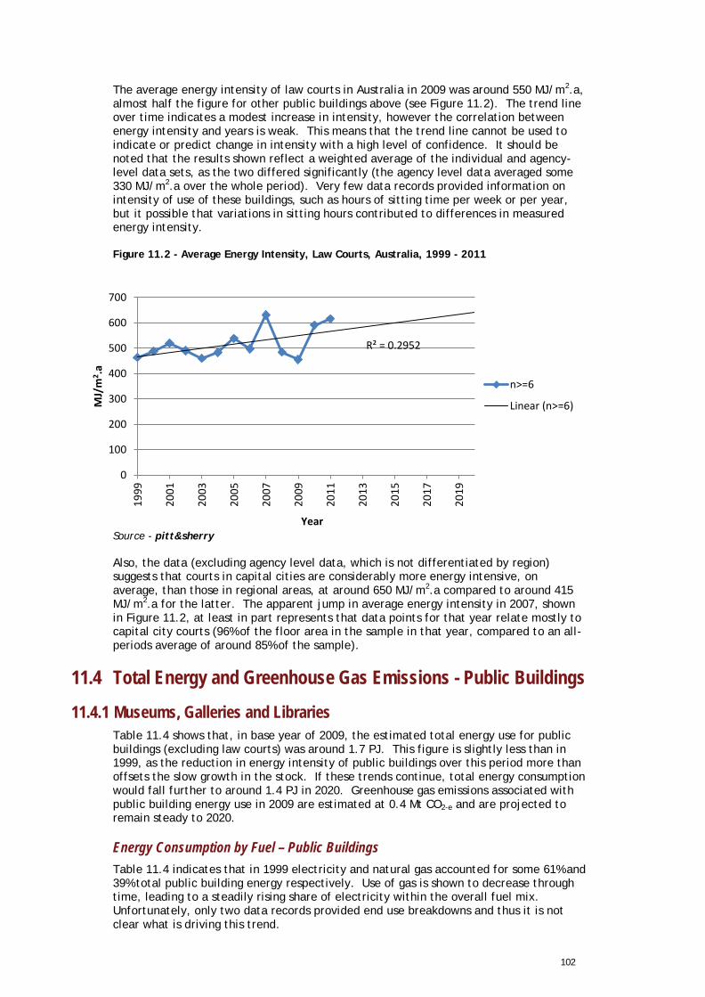
102

The average energy intensity of law courts in Australia in 2009 was around 550 MJ/m2.a, almost half the figure for other public buildings above (see Figure 11.2). The trend line over time indicates a modest increase in intensity, however the correlation between energy intensity and years is weak. This means that the trend line cannot be used to indicate or predict change in intensity with a high level of confidence. It should be noted that the results shown reflect a weighted average of the individual and agency-level data sets, as the two differed significantly (the agency level data averaged some 330 MJ/m2.a over the whole period). Very few data records provided information on intensity of use of these buildings, such as hours of sitting time per week or per year, but it possible that variations in sitting hours contributed to differences in measured energy intensity.

Figure 11.2 - Average Energy Intensity, Law Courts, Australia, 1999 - 2011

Source - pitt&sherry Also, the data (excluding agency level data, which is not differentiated by region) suggests that courts in capital cities are considerably more energy intensive, on average, than those in regional areas, at around 650 MJ/m2.a compared to around 415 MJ/m2.a for the latter. The apparent jump in average energy intensity in 2007, shown in Figure 11.2, at least in part represents that data points for that year relate mostly to capital city courts (96% of the floor area in the sample in that year, compared to an all-periods average of around 85% of the sample).

11.4 Total Energy and Greenhouse Gas Emissions - Public Buildings

11.4.1 Museums, Galleries and Libraries Table 11.4 shows that, in base year of 2009, the estimated total energy use for public buildings (excluding law courts) was around 1.7 PJ. This figure is slightly less than in 1999, as the reduction in energy intensity of public buildings over this period more than offsets the slow growth in the stock. If these trends continue, total energy consumption would fall further to around 1.4 PJ in 2020. Greenhouse gas emissions associated with public building energy use in 2009 are estimated at 0.4 Mt CO2-e and are projected to remain steady to 2020.

Energy Consumption by Fuel – Public Buildings Table 11.4 indicates that in 1999 electricity and natural gas accounted for some 61% and 39% total public building energy respectively. Use of gas is shown to decrease through time, leading to a steadily rising share of electricity within the overall fuel mix. Unfortunately, only two data records provided end use breakdowns and thus it is not clear what is driving this trend.

R² = 0.2952

0

100

200

300

400

500

600

700

1999

2001

2003

2005

2007

2009

2011

2013

2015

2017

2019

MJ/

m2 .a

Year

n>=6

Linear (n>=6)

103

Table 11.4 - Public Buildings, Energy Consumption by Fuel, and GHG Emissions, 1999 to 2020, Australia

Public Buildings:

Electricity Use (PJ)

Natural Gas Use

(PJ) LPG Use (PJ) Diesel/Oil

Use (PJ)

GHG Emissions (Mt CO2-e)

Total Energy Use (PJ)

1999 1.1 0.7 0.0 0.0 0.3 1.8

2000 1.1 0.7 0.0 0.0 0.4 1.9

2001 1.1 0.7 0.0 0.0 0.4 1.9

2002 1.2 0.7 0.0 0.0 0.4 1.8

2003 1.2 0.7 0.0 0.0 0.4 1.8

2004 1.2 0.6 0.0 0.0 0.4 1.8

2005 1.2 0.6 0.0 0.0 0.4 1.8

2006 1.2 0.6 0.0 0.0 0.4 1.7

2007 1.2 0.6 0.0 0.0 0.4 1.7

2008 1.2 0.5 0.0 0.0 0.4 1.7

2009 1.2 0.5 0.0 0.0 0.4 1.7

2010 1.2 0.5 0.0 0.0 0.3 1.7

2011 1.2 0.5 0.0 0.0 0.3 1.6

2012 1.2 0.4 0.0 0.0 0.3 1.6

2013 1.2 0.4 0.0 0.0 0.3 1.6

2014 1.2 0.4 0.0 0.0 0.3 1.5

2015 1.2 0.4 0.0 0.0 0.3 1.5

2016 1.2 0.3 0.0 0.0 0.3 1.5

2017 1.1 0.3 0.0 0.0 0.3 1.5

2018 1.1 0.3 0.0 0.0 0.3 1.4

2019 1.1 0.3 0.0 0.0 0.3 1.4

2020 1.1 0.3 0.0 0.0 0.3 1.4 Source - pitt&sherry

11.4.2 Law Courts Table 11.5 indicates that, in the base year of 2009, total energy consumption in law courts in Australia was around 0.6 PJ, about a 20% increase over the (low) 1999 base of just around 0.5PJ. Further modest growth to around 0.8 PJ is expected by 2020. Greenhouse gas emissions were similarly low, at around 100 kt CO2-e in 2009.

Energy Consumption by Fuel – Law Courts In term of fuel use, Table 11.5 indicates that law courts use close to 82% electricity, on average, and over 18% natural gas. While not shown in this table, the data available to NRBuild also indicates that very small amounts of LPG and diesel are used in courts, but less than 1 MJ/m2.a, on average, of either fuel.

11.5 Energy End Use - Public Buildings

11.5.1 Museums, Galleries and Libraries Energy end-use data was obtained for two public buildings only, which was not sufficient to undertake any meaningful analysis of energy energy-use.

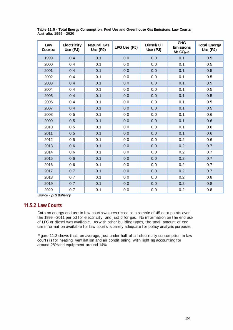
104

Table 11.5 - Total Energy Consumption, Fuel Use and Greenhouse Gas Emissions, Law Courts, Australia, 1999 – 2020

Law Courts:

Electricity Use (PJ)

Natural Gas Use (PJ) LPG Use (PJ) Diesel/Oil

Use (PJ)

GHG Emissions Mt CO2-e

Total Energy Use (PJ)

1999 0.4 0.1 0.0 0.0 0.1 0.5

2000 0.4 0.1 0.0 0.0 0.1 0.5

2001 0.4 0.1 0.0 0.0 0.1 0.5

2002 0.4 0.1 0.0 0.0 0.1 0.5

2003 0.4 0.1 0.0 0.0 0.1 0.5

2004 0.4 0.1 0.0 0.0 0.1 0.5

2005 0.4 0.1 0.0 0.0 0.1 0.5

2006 0.4 0.1 0.0 0.0 0.1 0.5

2007 0.4 0.1 0.0 0.0 0.1 0.5

2008 0.5 0.1 0.0 0.0 0.1 0.6

2009 0.5 0.1 0.0 0.0 0.1 0.6

2010 0.5 0.1 0.0 0.0 0.1 0.6

2011 0.5 0.1 0.0 0.0 0.1 0.6

2012 0.5 0.1 0.0 0.0 0.2 0.6

2013 0.6 0.1 0.0 0.0 0.2 0.7

2014 0.6 0.1 0.0 0.0 0.2 0.7

2015 0.6 0.1 0.0 0.0 0.2 0.7

2016 0.6 0.1 0.0 0.0 0.2 0.7

2017 0.7 0.1 0.0 0.0 0.2 0.7

2018 0.7 0.1 0.0 0.0 0.2 0.8

2019 0.7 0.1 0.0 0.0 0.2 0.8

2020 0.7 0.1 0.0 0.0 0.2 0.8 Source - pitt&sherry

11.5.2 Law Courts Data on energy end use in law courts was restricted to a sample of 45 data points over the 1999 – 2011 period for electricity, and just 6 for gas. No information on the end use of LPG or diesel was available. As with other building types, the small amount of end use information available for law courts is barely adequate for policy analysis purposes. Figure 11.3 shows that, on average, just under half of all electricity consumption in law courts is for heating, ventilation and air conditioning, with lighting accounting for around 28% and equipment around 14%.

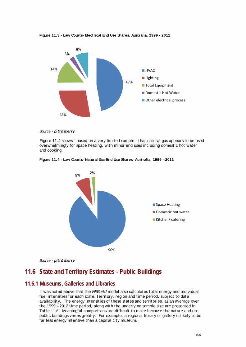
105

Figure 11.3 - Law Courts- Electrical End Use Shares, Australia, 1999 - 2011

. Source - pitt&sherry Figure 11.4 shows – based on a very limited sample - that natural gas appears to be used overwhelmingly for space heating, with minor end uses including domestic hot water and cooking. Figure 11.4 - Law Courts- Natural Gas End Use Shares, Australia, 1999 – 2011

. Source - pitt&sherry

11.6 State and Territory Estimates - Public Buildings

11.6.1 Museums, Galleries and Libraries It was noted above that the NRBuild model also calculates total energy and individual fuel intensities for each state, territory, region and time period, subject to data availability. The energy intensities of these states and territories, as an average over the 1999 – 2012 time period, along with the underlying sample size are presented in Table 11.6. Meaningful comparisons are difficult to make because the nature and use public buildings varies greatly. For example, a regional library or gallery is likely to be far less energy intensive than a capital city museum.

47%

28%

14%

3% 8%

HVAC

Lighting

Total Equipment

Domestic Hot Water

Other electrical process

90%

8% 2%

Space Heating

Domestic hot water

Kitchen/ catering

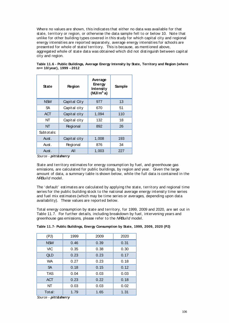
106

Where no values are shown, this indicates that either no data was available for that state, territory or region, or otherwise the data sample fell to or below 10. Note that unlike for other building types covered in this study for which capital city and regional energy intensities are reported separately, average energy intensities for schools are presented for whole of state/territory. This is because, as mentioned above, aggregated whole of state data was obtained which did not distinguish between capital city and region. Table 11.6 - Public Buildings, Average Energy Intensity by State, Territory and Region (where n>= 10/year), 1999 – 2012

State Region

Average Energy

Intensity (MJ/m2.a)

Sample

NSW Capital City 977 13

SA Capital city 670 51

ACT Capital city 1,094 110

NT Capital city 132 18

NT Regional 892 26

Subtotals: Aust. Capital city 1,008 193

Aust. Regional 876 34

Aust. All 1,003 227 Source - pitt&sherry State and territory estimates for energy consumption by fuel, and greenhouse gas emissions, are calculated for public buildings, by region and year. Given the large amount of data, a summary table is shown below, while the full data is contained in the NRBuild model. The ‘default’ estimates are calculated by applying the state, territory and regional time series for the public building stock to the national average energy intensity time series and fuel mix estimates (which may be time series or averages, depending upon data availability). These values are reported below.

Total energy consumption by state and territory, for 1999, 2009 and 2020, are set out in Table 11.7. For further details, including breakdown by fuel, intervening years and greenhouse gas emissions, please refer to the NRBuild model. Table 11.7- Public Buildings, Energy Consumption by State, 1999, 2009, 2020 (PJ)

(PJ) 1999 2009 2020

NSW 0.46 0.39 0.31

VIC 0.35 0.38 0.30

QLD 0.23 0.23 0.17

WA 0.27 0.23 0.18

SA 0.18 0.15 0.12

TAS 0.04 0.03 0.03

ACT 0.23 0.22 0.18

NT 0.03 0.03 0.02

Total: 1.79 1.65 1.31 Source - pitt&sherry

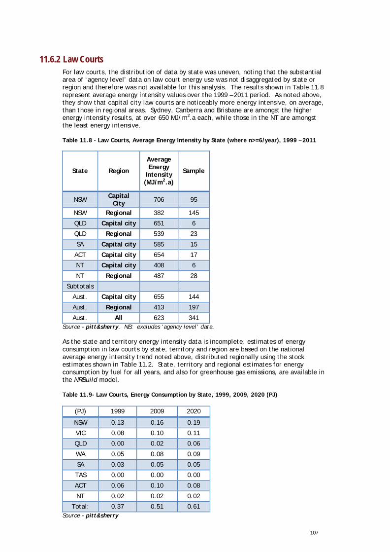
107

11.6.2 Law Courts For law courts, the distribution of data by state was uneven, noting that the substantial area of ‘agency level’ data on law court energy use was not disaggregated by state or region and therefore was not available for this analysis. The results shown in Table 11.8 represent average energy intensity values over the 1999 – 2011 period. As noted above, they show that capital city law courts are noticeably more energy intensive, on average, than those in regional areas. Sydney, Canberra and Brisbane are amongst the higher energy intensity results, at over 650 MJ/m2.a each, while those in the NT are amongst the least energy intensive. Table 11.8 - Law Courts, Average Energy Intensity by State (where n>=6/year), 1999 – 2011

State Region

Average Energy

Intensity (MJ/m2.a)

Sample

NSW Capital City 706 95

NSW Regional 382 145

QLD Capital city 651 6

QLD Regional 539 23

SA Capital city 585 15

ACT Capital city 654 17

NT Capital city 408 6

NT Regional 487 28

Subtotals Aust. Capital city 655 144

Aust. Regional 413 197

Aust. All 623 341 Source - pitt&sherry. NB: excludes ‘agency level’ data. As the state and territory energy intensity data is incomplete, estimates of energy consumption in law courts by state, territory and region are based on the national average energy intensity trend noted above, distributed regionally using the stock estimates shown in Table 11.2. State, territory and regional estimates for energy consumption by fuel for all years, and also for greenhouse gas emissions, are available in the NRBuild model. Table 11.9- Law Courts, Energy Consumption by State, 1999, 2009, 2020 (PJ)

(PJ) 1999 2009 2020

NSW 0.13 0.16 0.19

VIC 0.08 0.10 0.11

QLD 0.00 0.02 0.06

WA 0.05 0.08 0.09

SA 0.03 0.05 0.05

TAS 0.00 0.00 0.00

ACT 0.06 0.10 0.08

NT 0.02 0.02 0.02

Total: 0.37 0.51 0.61 Source - pitt&sherry

108

11.7 Conclusions - Public Buildings While it appears that public buildings, as defined, have been reducing their energy intensity through time, the conclusions in this study are based on a limited sample, with public buildings from Vic, Tas, WA and Qld not included in the data set. Second, it was noted that there appear to be differing energy intensities within the set, with larger, national institutions (galleries and museums) being more energy intensive, and libraries and less formal museums (such as motor and aircraft museums) being much less energy intensive. Ideally, these types of buildings would be modelled separately, although we note that the total energy consumption in public buildings is low, suggesting this may not need to be prioritised. Further, we note that this study has uncovered no statistically significant end use information for public buildings. We understand the Government Property Group may hold useful data with respect to public and government-owned buildings, but this data was not made available to this study. With respect to law courts, the analysis in this study is based on a large sample with only regional areas of some states unrepresented. We have noted that the study incorporates ‘agency level’ data that does not resolve individual buildings or states and also shows a much lower energy intensity than other data sources. This data set (from OSCAR) could be reviewed for accuracy, as recommended in Chapter 5. Finally, with respect to correctional centres, we note that data limitations prevented the construction of an energy module within NRBuild. Some data was captured for three correctional centres, although none of these records was complete. We note that with the co-operation of the states and territories, it should be possible to compile a more complete data set for correctional centres in future.

Appendix A - Statement of Requirements Appendix B - Bibliography Appendix C - Model Documentation Appendix D - Top-down Model Validation Appendix E - Statistical Analysis The above appendixes are in Part 2 of the publication.