© 2009 Key Curriculum Press 1

Barnsley’s Fractal Fern

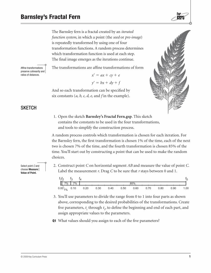
The Barnsley fern is a fractal created by an iterated

function system, in which a point (the seed or pre-image)

is repeatedly transformed by using one of four

transformation functions. A random process determines

which transformation function is used at each step.

The fi nal image emerges as the iterations continue.

The transformations are affi ne transformations of form

x� � ax � cy � e

y� � bx � dy � f

And so each transformation can be specifi ed by

six constants (a, b, c, d, e, and f in the example).

SKETCH

1. Open the sketch Barnsley’s Fractal Fern.gsp. This sketch

contains the constants to be used in the four transformations,

and tools to simplify the construction process.

A random process controls which transformation is chosen for each iteration. For

the Barnsley fern, the fi rst transformation is chosen 1% of the time, each of the next

two is chosen 7% of the time, and the fourth transformation is chosen 85% of the

time. You’ll start out by constructing a point that can be used to make the random

choices.

2. Construct point C on horizontal segment AB and measure the value of point C.

Label the measurement r. Drag C to be sure that r stays between 0 and 1.

85%7%7%

1%

t5

t4

t3

t2

t1

0.20 0.40 0.60 0.80 1.000.00 0.10 0.30 0.50 0.70 0.90

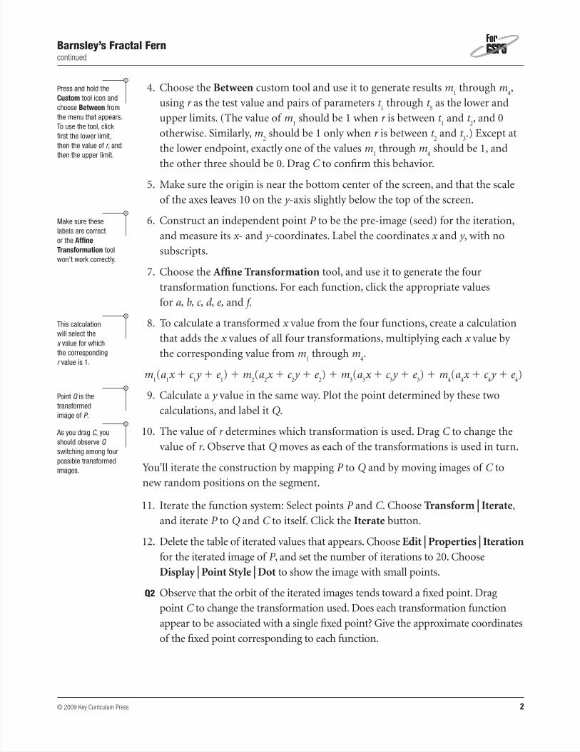
3. You’ll use parameters to divide the range from 0 to 1 into four parts as shown

above, corresponding to the desired probabilities of the transformations. Create

fi ve parameters, t1 through t

5, to defi ne the beginning and end of each part, and

assign appropriate values to the parameters.

Q1 What values should you assign to each of the fi ve parameters?

Affi ne transformations preserve colinearity and ratios of distances.

Select point C and choose Measure⏐Value of Point.

© 2009 Key Curriculum Press 2

Barnsley’s Fractal Fern continued

4. Choose the Between custom tool and use it to generate results m1 through m

4,

using r as the test value and pairs of parameters t1 through t

5 as the lower and

upper limits. (The value of m1 should be 1 when r is between t

1 and t

2, and 0

otherwise. Similarly, m2 should be 1 only when r is between t

2 and t

3.) Except at

the lower endpoint, exactly one of the values m1 through m

4 should be 1, and

the other three should be 0. Drag C to confi rm this behavior.

5. Make sure the origin is near the bottom center of the screen, and that the scale

of the axes leaves 10 on the y-axis slightly below the top of the screen.

6. Construct an independent point P to be the pre-image (seed) for the iteration,

and measure its x- and y-coordinates. Label the coordinates x and y, with no

subscripts.

7. Choose the Affi ne Transformation tool, and use it to generate the four

transformation functions. For each function, click the appropriate values

for a, b, c, d, e, and f.

8. To calculate a transformed x value from the four functions, create a calculation

that adds the x values of all four transformations, multiplying each x value by

the corresponding value from m1 through m

4.

m1(a

1x � c

1y � e

1) � m

2(a

2x � c

2y � e

2) � m

3(a

3x � c

3y � e

3) � m

4(a

4x � c

4y � e

4)

9. Calculate a y value in the same way. Plot the point determined by these two

calculations, and label it Q.

10. The value of r determines which transformation is used. Drag C to change the

value of r. Observe that Q moves as each of the transformations is used in turn.

You’ll iterate the construction by mapping P to Q and by moving images of C to

new random positions on the segment.

11. Iterate the function system: Select points P and C. Choose Transform⏐Iterate,

and iterate P to Q and C to itself. Click the Iterate button.

12. Delete the table of iterated values that appears. Choose Edit⏐Properties⏐Iteration

for the iterated image of P, and set the number of iterations to 20. Choose

Display⏐Point Style⏐Dot to show the image with small points.

Q2 Observe that the orbit of the iterated images tends toward a fi xed point. Drag

point C to change the transformation used. Does each transformation function

appear to be associated with a single fi xed point? Give the approximate coordinates

of the fi xed point corresponding to each function.

Press and hold the Custom tool icon and choose Between from the menu that appears. To use the tool, click fi rst the lower limit, then the value of r, and then the upper limit.

Make sure these labels are correct or the Affi ne Transformation tool won’t work correctly.

This calculation will select the x value for which the corresponding r value is 1.

Point Q is the transformed image of P.

As you drag C, you should observe Q switching among four possible transformed images.

© 2009 Key Curriculum Press 3

Barnsley’s Fractal Fern continued

13. The initial orbit that appears uses only a single transformation because the

images of C are not yet taking on new random positions. Select the iterated

image of P and choose Edit⏐Properties⏐Iteration. Change the number

of iterations to 5000, and click the radio button labeled Random locations on iterated paths.

14. Drag point C so the fourth function is used to generate point Q from P.

Q3 Move P to different locations on the fern, and describe the effect of this

transformation function in terms of the shape of the fern.

Q4 Similarly, activate each of the other transformation functions, and describe the

effect of these functions.

Q5 Where are the fi xed points of the four transformations in terms of the shape of

the fern?

Q6 Change the t parameters so the fi rst transformation is never used. What’s the

difference in the new shape? Describe the role of the fi rst transformation.

Q7 Determine and describe the role of each of the other transformations in

generating the image.

EXPLORE MORE

Q8 Determine the effect of the various constants in specifying the fern’s shape.

Q9 Modify the fern transformations so that the leaves of the fern are opposite each

other, instead of alternating.

Q10 Make other minor changes to the function system to produce a modifi ed

shape. (Be prepared to undo your changes—not all function systems generate

interesting results.)

Similar iterated function systems can generate a wide variety of fractals. For instance,

consider a system of three functions that have the following effects.

• Dilate the pre-image point by a scale factor of one-half toward the point (6, 0)

• Dilate the pre-image point by a scale factor of one-half toward the point (�6, 0)

• Dilate the pre-image point by a scale factor of one-half toward the point (0, 10)

Q11 Write down the transformation functions for these three transformations.

The image looks better with 10,000 iterations, if this number of iterations doesn’t slow your computer down too much.

To fi nd a fi xed point of a transformation, drag P until P and Q coincide.

© 2009 Key Curriculum Press 4

Barnsley’s Fractal Fern continued

Q12 Modify a copy of the fern sketch to use these transformations, with equal

probabilities for all three transformations. What fi gure results?

Q13 Build a similar iterated function system with four transformations, dilating the

pre-image by a factor of 0.44 toward one of the points (0, 0), (1, 0), (0, 1), (1, 1)

with equal probability. Describe the resulting fi gure.

Q14 Research Barnsley’s method and fractal compression. Report your fi ndings.