Fractal Antennae and Coherence

Juan A. ValdiviaCode 692,

Nasa Goddard Space Flight CenterGreenbelt, MD 20771

alejo@roselott.gsfc.nasa.gov(301) 286-3545

December 16, 1997

Abstract

Fractal antennae have very special properties:

(1) They are broad band antennae, i.e. they radiate, and detect, verye�ciently for a wide range of frequencies. The frequency range is speci�edby the smallest and largest size present in the antenna. The radiation,and hence the detection, e�ciency depends slowly on frequency betweenthese two limits.

(2) They can display considerable gain over normal dipole type of an-tennae and this gain depends slowly on frequency over a large frequencyrange. This antenna gain can be related to the spatio-temporal structureof the radiation pattern.

(3) They can display spatial structure. The spatial structure is alsorelated to the antenna gain, as the antenna concentrate radiated powerin certain postions and now in others. This spatial structure can be veryuseful when directionality is required.

1 Fractal Antennae and Coherence

For the purposes of this work, we assume that a fractal antenna can be formedas an array of "small" line elements having a fractal distribution in space. Suchdescription is consistent with our understanding of fractal discharges and light-ning observations as discussed by LeVine and Meneghini [1978], Niemeyer et

al. [1984], Sander [1986], Williams [1988], and Lyons [1994]. Appendix A de-velops the theory for the calculation of the �elds produced by a fractal antennacomposed of small line elements and for the calculation of the array factor inthe far �eld of the fractal.

1

Fractals are characterized by their dimension. It is the key structural pa-rameter describing the fractal and is de�ned by partitioning the volume wherethe fractal lies into boxes of side ". We hope that over a few decades in ", thenumber of boxes that contain at least one of the discharge elements will scale asN (") � "�D. It is easy to verify that a point will have D = 0, a line will haveD = 1 and a compact surface will have D = 2 . The box counting dimension[Ott, 1993] is then de�ned by

D 'lnN (")

ln(1")

(1)

For a real discharge there is only a �nite range over which the above scaling lawwill apply. If " is too small, then the elements of the discharge will look likeone-dimensional line elements. Similarly, if " is too large, then the discharge willappear as a single point. It is, therefore, important to compute D only in thescaling range, which is hopefully over a few decades in ". The fractal dimensionwill be an important parametrization for the fractal discharge models that wewill explore later, and will impact signi�cantly the intensity and spatial structureof the radiated pattern.

We consider a fractal antenna as a non uniform distribution of radiatingelements (Fig. 1). Each of the elements contributes to the total radiated powerdensity at a given point with a vectorial amplitude and phase, i.e.

E �E� � (NXn=1

Anei�n ) � (

NXm=1

Anei�m )� =

Xn;m

(An �A�m)e

i(�n��m) (2)

The vector amplitudes An represent the strength and orientation of each of theindividual elements, while the phases �n are in general related to the spatialdistribution of the individual elements over the fractal, e.g. for an oscillatingcurrent of the form ei!t the phases vary as � � kr where k = !

cand r is the

position of the element in the fractal.In the sense of statistical optics, we can consider the ensemble average of Eq.

(2), using an ergodic principle, over the spatial distribution P (�1; �2;�3;:::;A1;A2;A3; :::)of the fractal elements [Goodman, 1985]. For simplicity we assume that the dis-tributions for each of the elements are independent, and also the same, hence

G =NXn;m

D(An �A

�m)e

i(�n��m)E= N2(

DjAj2

EN

+N � 1

NjhAij

2 ��ei����2)By requiring that

DjAj

2E= jhAij

2= 1 we obtain that the ensemble average

is

hE �E�i � G = N2(1

N+N � 1

N

��ei����2)If the distribution of the phases is uniform (e.g. random) then < ei� >= 0 andG = 1=N . On the other hand, if there is perfect coherence we have < ei� >= 1

2

Figure 1: A spatially nonuniform distribution of radiators, each contributiongto the total radiation �eld with a given phase.

and G = 1. In general, a fractal antenna will display a power law distributionin the phases P�(�) � ��� (multiplied by the factor 1 � e��

��

so it is �niteat the origin), where � = 0 corresponds to the uniform distribution case and� ! 1 corresponds to perfect coherence. Figure 2 shows the plot of

��ei����as a function of �: It can be seen that a power law distribution of phases, orsimilarly a power law in the spatial structure, gives rise to partial coherence.

If the distribution of the vector amplitudes does not satisfy the above re-lations, e.g. the radiators are oriented in arbitrary directions, then the power

density will be less coherent due toDjAj2

E� jhAij2. A similar result can be

achieved by having a power law distribution in the amplitudes. In conclusion,the radiation �eld from a power law distribution of phases will have a pointwhere the phases from the radiators will add up almost (partially) coherentlyshowing a signi�cant gain over a random distribution of phases. Hence theconcept of a fractal antenna.

The partial coherence of the radiators depends on the spatial power lawdistribution. Such a power law distribution of phases can be visualized withthe help of Cantor sets [Ott, 1993]. A family of Cantor sets is constructed bysuccessively removing the middle � < 1 fraction from an interval, taken as [0,1],and repeating the procedure to the remaining intervals (see Fig. 3). At the nth

step, a radiator is placed at the mid-point of each of the remaining intervals.Note that for � = 0 we obtain a uniform distribution of elements, but for � 6=

0 the radiators are non-uniformly distributed, and in fact the spatial distributionfollows a power law that can be described by its fractal dimension. Suppose thatfor " we require N (") intervals to cover the fractal, then it is clear that with"0

! "2(1 � �) we would require 2N ("

0

) intervals to cover the fractal. But the

3

2 4 6 8 10a

0.2

0.4

0.6

0.8

1

» < E >»2

N2

Figure 2: A plot of��ei����2 as a function of �.

fractal is the same, therefore, N (") = 2N ("0

). From the scaling N (") � "�D weobtain that the dimension is given by

D = �ln 2

ln(1��2 )

We can go further, and write a formula for the radiation �eld due to the��Cantor set of radiators. Note that if at the nth step we have the radiatorsplaced at the sequence of points Sn = fxiji = 1; :::; 2n�1g then at the nth+1 stepeach radiator at xi will be replaced by two radiators at xi�

12n+1 (1��)

n�1(1+�)generating the sequence Sn+1 = fxiji = 1; :::; 2ng. Since we start with S1 = f12gthe sequences Sn at the nth step are trivially constructed. The radiation �eld(see Eq. (1)) from this ��Cantor set at the nth step can then be written as

E =nX

m=1

(�1)m�meikLa xm+i�m (3)

where k = !c, L is the spatial extent of the fractal, a = bx � br is the angular

position of the detector, and �m (taken as zero) is the phase of the mth element.The radiators are given a strength proportional to the measure �i (or length)of the segment which de�nes it.

The space dependence of the radiation �elds is plotted in Fig. (4)a-b for� = 1=3 (D = 0:63) and � = 0 (D = 1) respectively, where the sets have beentaken to the 5th level. The most relevant issue for our purposes is the fact thatthere is a direction at which phases add coherently (partially) for � = 1=3 whilethis does not happen for the homogeneous case � = 0.

4

AND SO ON

Figure 3: The construction of the fractal distribution of the radiators from the��Cantor set.

-6 -4 -2 2 4 6 2pkLa

0.5

1

1.5

2

2.5

3E2 h=1ê6 D=0.63

-6 -4 -2 2 4 6 2pkLa

0.5

1

1.5

2

2.5

3E2 h=0 D=1

Figure 4: The spatial dependence of the radiation �elds for (a) � = 1=3, D =0:63 and (b) � = 0, D = 1.

Therefore, partial coherence occurs naturally in systems that have power-law spatial distributions. We are now ready to turn to the properties of fractalantennae with propagating currents. Speci�cally, how tortuosity and branchingcan increase the radiated �eld intensity in some locations as compared withsingle dipole antennae.

2 Radiation and Simple Fractal Models

To illustrate the properties of fractal antennae compared to those of simpledipole radiators, we take the fractal antenna as composed of small line elementsand compute its far �eld radiation pattern. For an oscillating current I(t) =Ioe

�i!t that propagates with speed � =v/c along the antenna, the contribution

5

from each line element to the total radiation �eld is (from Eq. (1))

crEn(r; t)

Io= e�i!teikr

�bLn(1� �an)

eikpnbneiksn� (eikLnanei

kLn� � 1) (4)

where an = bLn�br, pn is the position of the beginning of the line element from theorigin, and bn = bpn �br. Radiation occurs when there is a change in the directionof the propagating current. Also note that mathematically we can describe aradiator with a nonpropagating current in the non-physical limit � !1.

In general, the radiation pattern of an antenna can be e�ectively excited,only by certain frequencies corresponding to the characteristic length scales ofthe antenna, e.g. kL � 1 (see Eq. (4)). Therefore, if there is no characteristicsize, as in the case of a power law structure, then the antenna will generatean e�ective radiation pattern for a whole range of frequencies controlled by thesmaller and largest spatial scale. Such antenna is called a broad band antenna,and that is why fractal antennae are so important in many applications.

By spatially superposing these line radiators we can study the propertiesof simple fractal antennae. Of special interest, to our high altitude lightningwork, is to compare the radiation pattern of these fractal models with a simple(meaning one line element) dipole antenna.

2.1 Gain Due to Tortuosity

The �rst element in understanding fractal antennae is the concept of tortuosityin which the path length between two points is increased by requiring that thesmall line elements are no longer colinear. A simple tortuous model is displayedin Fig. 5, where the parameter " represents the variation from the simple dipolemodel (line radiator), i.e. the dipole is recovered as "! 0.

Except for the propagation e�ect, we can observe that this antenna (Fig. 5)can be considered as the contribution from a long line element (a dipole) plus thecontribution from a Cantor set of radiators as described in the previous section(see Eq. (3)). Therefore, the tortuosity naturally increases the radiation �eldintensity, at least in some direction, as compared with the single dipole element.

The �eld can be written for the structure of 5, with the help of Eq. (4), asthe superposition of the 2N line elements, and is given by the normalized �eld

E(") =�(eiklaxei

kl� � 1)

(1� �ax)bx+ �eiklaxei

kl� (eik"ayei

"kl� � 1)

(1� �ay)by + : : : (5)

where l = LN

is the length of the small segments composing the tortuous path,and ax = bx � br and ay = by � br. It is clear that in the limit "! 0 we recover thesingle dipole radiation pattern. The e�ect of the tortuosity can now be posedas the behavior of the normalized P(") = E(") �E�(") for " 6= 0. In general theanalysis can be simpli�ed in the limit for small ", i.e. P(") ' P(0)+P0(0)"+ : : :.Of course P(0) is the dipole contribution, and P0(0)" is the change in the radiatedpower density due to tortuosity. The dipole has a maximum in the radiated

6

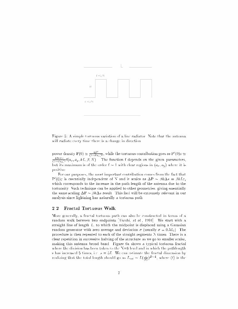
Figure 5: A simple tortuous variation of a line radiator. Note that the antennawill radiate every time there is a change in direction.

power density P(0) ' 4�2

(1��ax)2, while the tortuous contribution goes as P0(0)" '

4�kL"(1��ax)2

f(ax; ay; kL; �;N ) . The function f depends on the given parameters,

but its maximum is of the order f � 1 with clear regions in (ax; ay) where it ispositive.

For our purposes, the most important contribution comes from the fact thatP0(0)" is essentially independent of N and it scales as �P � �k�s = �kL";which corresponds to the increase in the path length of the antenna due to thetortuosity. Such technique can be applied to other geometries, giving essentiallythe same scaling �P � �k�s result. This fact will be extremely relevant in ouranalysis since lightning has naturally a tortuous path.

2.2 Fractal Tortuous Walk

More generally, a fractal tortuous path can also be constructed in terms of arandom walk between two endpoints [Vecchi, et al., 1994]. We start with astraight line of length L, to which the midpoint is displaced using a Gaussianrandom generator with zero average and deviation � (usually � = 0:5Li). Theprocedure is then repeated to each of the straight segments N times. There is aclear repetition in successive halving of the structure as we go to smaller scales,making this antenna broad band. Figure 6a shows a typical tortuous fractalwhere the division has been taken to the N=8 level and in which the pathlengths has increased 5 times, i.e. s = 5L. We can estimate the fractal dimension byrealizing that the total length should go as Ltot � L( s

h`i )D�1, where h`i is the

7

average segment size. This formulation is completely equivalent to Eq. (1).We let an oscillating current, e.g. Ioei!t; propagate along the fractal, but in

real applications we can imagine the oscillating current lasting for only a �nitetime 1=�. In order to have a �nite current pulse propagating through the fractalrandom walk, we let I(t) = Io(e��t�e� t)(1+cos(!t))�(t) with ! = 2��nf and�(t) as the step function. Here nf represent the number of oscillations duringthe decay time scale 1/� . We chose the decay parameters as � = 103 s�1 and = 2 � 105 s�1, hence =� = 200, which correspond to realistic parametersfor lightning [Uman, 1987]. The radiated power density is then computed usingEq. (12) and is shown in Fig. 6b for nf = 5 and � = 0:1 at the position ax = 0,ay = 0; r = 60 km. The dipole equivalent is given by the dashed lines in all 3panels. The peak in the radiated power density is about 10 times larger than for

the dipole case, which agrees well with the results P0(0)"P(0) � 2���s

c�nf � 10 even

though the e�ect from the tortuosity is not small. The larger path length ofthe tortuous discharge produces an increase in the radiation as compared witha dipole radiator. Of course there is a limit due to energy conservation, but inpractical applications we are well under it. The increase in the high frequencycomponents of the radiated �eld power spectrum (Fig. 6c), as compared withthe dipole antenna, will be responsible for the spatially structured radiationpattern.

Figure 6: The fractal random walk (a) and its instantaneous radiated powerdensity (b) as well as its power spectrum (c). The dashed lines represent thebehavior of the single dipole.

The far �eld array factor R = �RdtE2 (de�ned in Appendix A) and the

8

peak power density depend on the path length, or equivalently on the numberN of divisions of the fractal. Figure 7b shows the array factor as a function ofthe path length for the fractal shown in Fig. 7a. Here nf = 5 so that the peakof the array factor is at ax = 0 and ay = 0. There is a clear increase in the arrayfactor from the tortuous fractal as compared with the single dipole.

Figure 7: (a) The tortuous discharge. (b) The array factor dependence, nor-malized to the dipole, on the pathlength.

Therefore, the e�ect of tortuosity can increase the radiated power density atcertain locations as compared to a single dipole antenna.

Another important concept related to fractal antennae is the spatial struc-ture of the radiation �eld. We can see from the array factor, Eq. (13), thatfor large nf f [�; �] ' e�� (2 + cos(�� )). The spatial dependence of the array

factor will be determined by the factor ���r

cover the fractal. Consequently, the

radiation pattern will have spatial structure when ���r

c> 2�; which translate

into nf > 50. Figure 8b shows the array factor at the height h = 60 km for thedischarge structure shown in Fig. 8a with nf = 200. Therefore, such a tortu-ous fractal can also display a spatial structure in the radiation pattern. But itis more natural for the spatial structure to be generated through a branchingprocess as we will see in the next section.

There is an energy constraint that limits the degree of tortuosity of a fractallightning discharge since we cannot radiate more energy than what is initiallystored as separated charge. Also, if the line elements of the antenna given by Fig.5 get too close together, then their contribution to the radiated �eld will tendto cancel each other. Therefore, there is an optimal number of elements forming

9

Figure 8: The fractal structure (a) and its array factor(b) showing clear spatialstructure in the radiation pattern.

an antenna, and this optimal number translates into an optimal dimension ofthe fractal, more on this later.

2.3 Branching and Spatial Structure

Another element in understanding fractal antennae is the concept of branching.Take the simple branching element shown in Fig. 9 where the current is dividedbetween the two branching elements. We can compute the radiation �eld, for apropagating current Ioei!t, as

E(") = bx�(eik`axei k`� � 1)

(1� �ax)+by�eik`axei k`�

(1� �ay)

1

2f(eik`"ayei

"k`� �1)�(e�ik`"ayei

"k`� �1)g : : :

(6)where ` = L=2 and " is the variation from the single dipole, i.e. we recover thedipole as "! 0.

Again, the analysis can be simpli�ed in the limit for small ", i.e. P(") 'P(0) + P0(0)" + : : : . Of course P(0) is the dipole contribution, and P0(0)"

10

Figure 9: A simple branching situation in which we distribute the current amongthe branching elements.

is the change in the radiated power density due to the line branching. The

dipole has a maximum in the radiated power density P(0) ' 4�2

(1��ax)2, while

the branching contribution goes as P0(0)" ' �kL"

(1��ax)2f(ax; ay; kL; �;N ). The

function f depends on the given parameters, but its maximum is of the orderf � 1 with clear regions in (ax; ay) where it is positive. Therefore, the branchingprocess can give rise to an increase in the radiated power density at certainposition. Of course this increase is due to the increase in the path length.This e�ect will saturate as " is increased passed one, since then the strongestcontribution will come from the dipole radiator given by 2"L.

A interesting and manageable broadband antenna can be described in termsof the Weierstrass functions [Werner and Werner, 1995]. We take successivebranching elements, as shown in Fig. 10a, where we distribute the current ateach branching point so that the branching element keeps a fraction � of thecurrent. The nth branching element is displaced by a factor "n with respect tothe origin. If we concentrate only on the contribution from the last branchingset, as shown in Fig. 10a, we can write the �eld as

Ex �NXn=1

"n(do�2) cos(kl"nay + �n(�))

�n(�) =kl

�"n�1(2 + ")

where we have rede�ned � = "do�2 and ay = cos � . In the limit � !1 and N!1 we obtain the Weierstrass function that is continuous but not di�erentiable,i.e. is a fractal, and furthermore, its dimension in the sense given by Eq. ( 1)is do. For the purpose of illustration we truncate the above sum to N = 8. InFig. 10b, we show the dependence of the �eld as a function of ay � [�1; 1] withax = 0 for � ! 1. The parameters values are shown in the �gure caption.

11

Figure 10c shows the gain factor given by

G =max jEj2

12

Rday jEj

2

as a function of the dimension do � [0; 1]. We chose this range since the fractalalready has a dimension 1 in the perpendicular directions, i.e. D=1+do.

Figure 10: The branching process to produce a Weierstrass radiation pattern.(a) The brunching process with the branching length increasing as "nL and thecurrent decreasing as �nIo. (b) the radiation pattern with � !1 given perfectcoherence. (c) The gain vs the dimension. It also contains the parameters usedin all 3 �gures. (d) Patial coherence for � = 0:1.

Note the increase in the gain as a function of dimension. In general, there isan optimal value of D that generates the highest power density and that doesnot necessarily has to be for D = 2. In Fig. 10b all the elements from theantenna add up coherently at ay = 0, hence providing perfect coherence. Fora �nite � < 1 the propagation brings a di�erent phase shift at each element.Figure 10d shows the e�ect for � = 0:1 as a function of �. Note that at no pointthere is perfect coherence, but there is clear partial coherence. The peak valueof E2 is actually sensitive to �.

12

Even though fractal antennae naturally lead to the concept of an increasein the peak radiated power, it also has a second important consequence dueto branching. As we have seen in the case of the Wiertrauss function, fractalantennae naturally result in the generation of a spatial structure in the radiatedpower density. This interplay between the spatial structure and the increase inthe peak radiated power are the essential ingredients of fractal antennae andwhy they are so important. A clear example can be illustrated in Fig. 10dwhere there are multiple relevant peaks of the radiated power in space.

3 Modeling Lightning as a Fractal Antenna

The hypothesis of this work is that the structure of the red sprites can beattributed to the fact that the power density generated by lightning does nothave the smooth characteristics expected from the dipole model of Eq. 7, butthe structured form expected from a fractal antenna [ Kim and Jaggard, 1986;Werner et al., 1995]. Previous studies of lightning assumed that the RF �eldscausing the atmospheric heating and emissions, were produced by an horizontaldipole cloud discharge moment M that generates an electric �eld at the heightz, given by

E =M

4��oz3+

1

4��ocz2dM

dt+

1

4��oc2z

d2M

dt2(7)

where c is the velocity of light and �o is the permitivity of free space. It is im-portant to realize that a lightning discharge must be horizontal, as in intracloudlightning, to project the energy upwards into the lower ionosphere. A verticaldischarge, as in cloud-to-ground lightning, will radiate its energy horizontallyas a vertical antenna.

It is obvious that such a horizontal dipole results in electric �elds that varysmoothly with distance. However, it is well known that lightning dischargesfollow a tortuous path [LeVine and Meneghini, 1978]. It was shown [ Williams,1988] that intracloud discharges resemble the well known Lichtenberg patternsobserved in dielectric breakdown. In fact a time-integrated photograph of a sur-face leader discharge is illustrated by Figure 11 . These patterns have been re-cently identi�ed as fractal structures of the Di�usion Limited Aggregate (DLA)type with a fractal dimension D � 1:6 [Sander, 1986; Niemeyer et al., 1984].

As noted previously, the tortuous path increase the e�ective dipole moment,since now the pathlength along the discharge is longer that the Euclidean dis-tance. To understand this analogy, we construct a tortuous walk between twopoints separated by a distance R as shown in Fig 12. Take the tortuous pathas N small steps of averaged step length Lo � R, then the total path length Salong the tortuous discharge is

S � NLo � (R

Lo)D�1R

where the number of small steps is N � ( RLo)D with D as the box counting

dimension [Ott, 1993]. As we have seen before, the change in the path length

13

Figure 11: Time-integrated photograph of a surface leader discharge (Lichten-berg pattern) [Niemeyer et al., 1984]

increases the radiated power density as E2 = E2o + �k(S � R) where E2

o � �2

Therefore, for R � 10 km (typical for an intracloud discharge), Lo � 50 m,

� = 0:1, and D � 1:6, with obtain E2

E2o� 1 + kR

�(( R

Lo)D�1 � 1) � 1 + 5f(kHz)

where f is the frequency of the current.This is only an analogy, but it gives us good intuition that a fractal lightning

discharge will produce an increase in the radiated �eld intensity, at least locally,as compared with a dipole model and a spatially structured radiation pattern.A fractal dielectric discharge of size R can be modeled as a set of non-uniformlydistributed small current line elements [ Niemeyer et al., 1984] that representthe steps of the discharge breakdown as it propagates during an intracloudlightning discharge. The size of the elementary current steps is about Lo � 50m [Uman, 1987]. As a current pulse propagates along this horizontal fractaldischarge pattern it radiates energy upwards (see Appendix A on how the �eldsare calculated) as well as downward.

To determine the extent over which the non-uniformity of the lightning dis-charge current a�ects the power density structure projected in the lower iono-sphere, we will now construct a simple fractal model of the lightning dischargethat will yield a spatio-temporal radiation pattern at the relevant heights.

3.1 Fractal Lightning: Stochastic Model

We want to generate a fractal model that can be parametrized by its fractal di-mension. For this purpose, we followNiemeyer et al. [1984] who proposed a two

14

Figure 12: Tortuous path between two point.

dimensional stochastic dielectric discharge model that naturally leads to fractalstructures. In this model the fractal dimension D can be easily parametrizedby a parameter �. Femia et al. [1993] found experimentally that the propa-gating stochastic Lichtenberg pattern is approximately an equipotential. Then,the idea is to create a discrete discharge pattern that grows stepwise by addingan adjacent grid point to the discharge pattern generating a new bond. Thenew grid point, being part of the discharge structure, will have the same poten-tial as the discharge pattern. Such local change will a�ect the global potentialcon�guration, see Fig. 13.

The potential for the points not on the discharge structure is calculated byiterating the discrete two dimensional Laplace's equation

r2� = 0�i;j =

14 (�i+1;j + �i�1;j + �i;j+1 + �i;j�1)

until it converges. This method reproduces the global in uence of a given dis-charge pattern as it expands. The discharge pattern evolves by adding an ad-jacent grid point. The main assumption here is that an adjacent grid pointdenoted by (l,m) has a probability of becoming part of the discharge patternproportional to the � power of the local electric �eld, which translates to

p(i; j) =��i;jPl;m

��l;m

in terms of the local potential. Here we have assumed that the potential atthe discharge is zero. The structure generated for � = 1, corresponding to aLichtenberg pattern, is shown in Fig. 14.

15

������

������������

������

������

������

���

������

������

���

������

������

���

���

���

������

���

���

���

������

������

������

������

Figure 13: Diagram of the discrete discharge model.

The color coding corresponds to the potential. Figure 15 shows a plot ofN (") vs. Log(") for the fractal discharge of Fig. 14, i.e. � = 1:0. Againthe scaling behavior only occurs over a few decades, but it is very clear. Thedimension of this structure is D ' 1:6.

Note that this model, and also the dimension of the discharge, is parametrizedby �. Intuitively we expect that when � = 0 the discharge will have the sameprobability of propagating in any direction, therefore, the discharge will be acompact structure with a dimension D = 2. If � ! 1 then the discharge willgo in only one direction, hence D = 1. Between these two limits, the dimensionwill be the function D(�) shown in Fig 16. As an example the correspondingstructure generated for � = 3 (Fig 17) has a dimension of D = 1:2.

To compute the radiated �elds, we must describe the current along each ofthe segments of the fractal discharge. We start with a charge Qo at the centerof the discharge. The current is then discharged along each of the dendriticarms. At each branching point we chose to ensure conservation of current, butintuitively we know that a larger fraction of the current will propagate alongthe longest arm. Suppose that a current Io arrives at a branching point, andif Li is the longest distance along the ith branching arm, we intuitively expectthat the current on the ith arm should be proportional to L�i . Therefore, wesatisfy charge (or current) conservation if the current along the ith branchingarm is

Ii =L�iPj L

�j

16

Figure 14: Fractal discharge generated with � = 1.

3.2 Computing the Fields from the Fractal Structure

A current pulse propagates along the horizontal (in the x-y plane) 2 dimensionalfractal discharge structure, e.g. I(x; t) = I(t � s

v ) generating radiation �elds.The radiation �eld is the superposition, with the respective phases, of the smallline current elements. The intracloud current pulse is taken as a series of trainpulses that propagate along the arms of the antenna

I(t) = Io(e��t � e� t)(1 + cos(!t))�(t)

with ! = 2��nf and �(t) as the step function. Here nf represent the numberof oscillations during the decay time scale 1/�. We chose the decay parametersas � = 103 s�1 and = 2 � 105 s�1, hence =� = 200, which correspond torealistic parameters for lightning [Uman, 1987]. The total charge discharged isthen Q = Io=�, which for Io = 100 kA gives Q � 100 C. As we have seen before,we require nf � 100 to create the spatial structures so that the exponentialdecay e��t can be considered as the envelope of the oscillating part.

On a given position the time dependence of the �eld intensity E2 has afractal structure, as it is shown in Fig. 18a for the stochastic discharge modelwith � = 3. The frequency spectrum of the electric �eld is shown in Fig.18b. It is very important to realize that the relevant frequencies are below afew hundred kHz. By restricting the �eld frequencies to below a few hundredkHz, the analysis is greatly simpli�ed, since then the conductivity and dielectrictensors can be considered as independent of time in the lower ionosphere (seeAppendix B).

The large conductivity of the ground at these frequencies can be included byassuming to �rst order an image discharge of opposite current below a perfectly

17

Figure 15: The plot of lnN (�) vs 1�for � = 1.

conductive plane. The primary discharge is taken to be at zo = 5 km above theground. This parameter is not very relevant, since we are interested in the �eldat heights of about h � 80 km, therefore, moving the discharge from 5 to 10 kmwill only change the �eld strength by a marginal 10%.

3.3 How does the Fractal Dimension A�ect the Field Pat-tern?

For a 2-dimensional fractal structure, we expect that the strength of the radiatedpower density depends on the fractal structure, i.e. its fractal dimension. If thestrength of the k Fourier component is Ak then the �eld in the far �eld [ Jackson1975] at r along the axis of the fractal will be given by

E �

ZdkAk

Z�

d�R(�) sin(k�)

where d� (the fractal measure) is the contribution of the fractal from a givenpolar position (�,�). R(�) is the phase contribution from the elements of thefractal at position (�,�) and in the far �eld should be proportional to the direc-tion of the local current. Note that a radially propagating uniform 2 dimensionalcurrent structure will generate no �eld at the axis since contributions to R(�)from di�erent parts of the fractal will cancel each other.

The cross section of the fractal at a given radius � will resemble a Cantor setin � � [0; 2�], and the phase contribution will be given by S(�) =

R�d�R(�; �)

which will be �nite for an asymmetrical fractal. The integration can be carried asa Lebesgue integral or as a Riemann-Stieltjes integral over this pseudo-Cantor

18

Figure 16: The dimension of the stochastic model as a function of � with theestimated error bars.

set [Royden, 1963]. Note that if the fractal is uniformly distributed along �,corresponding to D=2, then S(�) = 0. Similarly, for a delta function at � =�o corresponding to D=1, S(�) gives a positive contribution. S(�) is a verycomplicated function that depends on the details of the current distributionalong the fractal. In an average sense we can suppose that S(�) � f(D) wheref(D = 1) = 1 and f(D = 2) = 0 but f can be greater than one for other valuesas has been investigated in previous sections when branching and propagationoccurs. Therefore,

E�f(D)

ZdkAk

Z�

dm(�) I(�) sin(k�)

where dm(�) represents the amount of the fractal between � and � + d� andI(�) is the averaged current over � at radius �. A fractal will have a mass upto a radius � given by m(�) = ( �

Lo)D by noting that a 2 dimensional antenna

will have more elements than a one dimensional fractal. In general, due to thebranching process, some of the current does not reach the radius R. But forsimplicity, if all of the current reaches the end of the fractal at radius R, thendm(�) I(�) = d�. In such case, the above integral gives

E�f(D)

Zdk k�1Ak(1 � cos(kR))

19

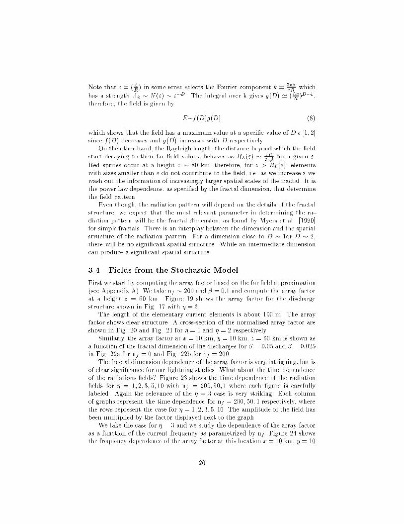
Note that " = ( `R) in some sense selects the Fourier component k = 2��

"Rwhich

has a strength Ak � N (") � "�D . The integral over k gives g(D) ' (LoR)D�1;

therefore, the �eld is given by

E�f(D)g(D) (8)

which shows that the �eld has a maximum value at a speci�c value of D � [1; 2]since f(D) decreases and g(D) increases with D respectively.

On the other hand, the Rayleigh length, the distance beyond which the �eldstart decaying to their far �eld values, behaves as RL(") �

"R2�� for a given ".

Red sprites occur at a height z � 80 km, therefore, for z > RL("); elementswith sizes smaller than " do not contribute to the �eld, i.e. as we increase z wewash out the information of increasingly larger spatial scales of the fractal. It isthe power law dependence, as speci�ed by the fractal dimension, that determinethe �eld pattern.

Even though, the radiation pattern will depend on the details of the fractalstructure, we expect that the most relevant parameter in determining the ra-diation pattern will be the fractal dimension, as found by Myers et al. [1990]for simple fractals. There is an interplay between the dimension and the spatialstructure of the radiation pattern. For a dimension close to D � 1or D � 2,there will be no signi�cant spatial structure. While an intermediate dimensioncan produce a signi�cant spatial structure.

3.4 Fields from the Stochastic Model

First we start by computing the array factor based on the far �eld approximation(see Appendix A). We take nf � 200 and � = 0:1 and compute the array factorat a height z = 60 km. Figure 19 shows the array factor for the dischargestructure shown in Fig. 17 with � = 3.

The length of the elementary current elements is about 100 m. The arrayfactor shows clear structure. A cross-section of the normalized array factor areshown in Fig. 20 and Fig. 21 for � = 1 and � = 2 respectively.

Similarly, the array factor at x = 10 km, y = 10 km, z = 60 km is shown asa function of the fractal dimension of the discharges for � = 0:05 and � = 0:025in Fig. 22a for nf = 0 and Fig. 22b for nf = 200.

The fractal dimension dependence of the array factor is very intriguing, but isof clear signi�cance for our lightning studies. What about the time dependenceof the radiations �elds? Figure 23 shows the time dependence of the radiation�elds for � = 1; 2; 3; 5; 10 with nf = 200; 50; 1 where each �gure is carefullylabeled. Again the relevance of the � = 3 case is very striking. Each columnof graphs represent the time dependence for nf = 200; 50; 1 respectively, wherethe rows represent the case for � = 1; 2; 3; 5; 10. The amplitude of the �eld hasbeen multiplied by the factor displayed next to the graph.

We take the case for � = 3 and we study the dependence of the array factoras a function of the current frequency as parametrized by nf : Figure 24 showsthe frequency dependence of the array factor at this location x = 10 km, y = 10

20

km, z = 60 km. Initially the array factor increases linearly with nf as expectedbut then it starts to oscillate as the spatial variation of the �eld pattern becomesrelevant.

In conclusion, the fractal nature of the discharges, being a simple randomwalk or a stochastic discharge model, leads naturally to an increase in the peakpower density as compared with the dipole model. This increase is related to theincrease in the antenna path length, or tortuosity, and on the branching process.It will be shown later that this gain in peak power density leads to a signi�cantreductions in the discharge properties (e.g. charge, peak current) required toproduce the observed sprite emissions. Furthermore, if the discharge has a highfrequency component, as expected from an acceleration and deceleration processin each of the single steps, then the radiation pattern can show spatial structure.This spatial structure of the lightning induced radiation pattern will be relatedto the spatial structure of the red sprites in the next chapter.

4 Appendix A: Fields from a Fractal Structure

The �elds from a line element can be solve with the help of the Hertz Vector[Marion and Heald, 1980]. In order to solve Maxwell's equations we de�ne, inempty space, the vector function Q [ Marion and Heald, 1980] that is relatedto the current density J and the charge density � as

J = �@Q

@t

� = r �Q

Note that Q solves the continuity equation trivially, and furthermore, it can beused to de�ne another vector function, namely the Hertz vector �(x; t); as

r2��1

c2@2�

@t2= �4�Q

where the �elds are then de�ned as

B(x; t) =1

cr�

@�(x; t)

@t

E(x; t) = r�r��(x; t)

The time-Fourier transformed Maxwell's equations, with Q(x; !) = i!J(x; !)

and J(x; !) = bLI(l; !); can be solved with the help of the Hertz vector �,

�(x; !) =i

!

Z L

0

J(l; !)eik

x�lbL x�lbL dl (9)

where the line element has orientation L and length L, and is parametrized byl � [0; L]. Values with the hatb indicate unit vectors, variables in bold indicatevectors, ! is the frequency, k = !

c. The time dependence can be found by

inverting the above equation.

21

4.1 Fields from a Fractal Antennae

A current pulse propagates with speed � = vcalong a fractal structure. At the

nth line element with orientation Ln and length Ln, which is parametrized byl � [0; Ln], the current is given by I(l; sn; t) = Io(t�

sn+lv ) where sn is the path

length along the fractal (or if you prefer a phase shift). The radiation �eld isthe superposition, with the respective phases, of the small line current elementsthat form the fractal. For a set frn;Ln; I(sn; t) jn = 0; :::; Ng of line elements,such as shown in the example diagram of Fig. 25, the Hertz vector is given by

�(x; !) =Xfng

bLn i

!

Z Ln

0

Io(!)ei!v(sn+l) e

ikkrn�lbLnkk rn � lbLn kdl (10)

where rn is the vector from the beginning of the nth line element to the �eldposition x, ! is the frequency and k = !

c.

We must realize that in general Eq. 10 for � is very complicated, but weare interested in the far �eld of the small line elements (rn � L). Therefore,we can take the far �eld approximation of the small line elements to obtain aclosed form solution for the Fourier transformed �elds as

B(x; !) = �Xfng

k2eikrn

rnf(sn; !; rn)[1 +

i

(krn)](bLn � brn)

E(x; !) = �P

fngk2eikrn

rnf(sn; !; rn)[(1 +

i(krn)

+ i2

(krn)2)cLn

�brn(bLn � brn)(1 + 3i(krn)

+ 3i2

(krn)2]

where the geometric factor is given by

f(sn; !; rn) =i

!

Z Ln

0Io(sn; l; !)e

�i(bLn�brn)kldl = ieicvsn

!Io(!)

Z Ln

0ei(

cv�(bLn�brn)k)ldl

f(sn; !; rn) =�Io(!)ei

!vsn

ck2(1� �(bLn � brn)) (1� ei(cv�(bLn�brn)k)Ln)

Note that even though we are in the far �eld of the small line elements, wecan be in fact in the intermediate �eld with respect to the global fractal struc-ture. Therefore, phase correlations over the fractal can be extremely relevant,and produce spatially nonuniform radiation �elds. We then invert the Fouriertransform of the �eld to real time and obtain the spatio-temporal radiationpattern due to the fractal discharge structure

B(x; t) =Xfng

�(bLn � brn)crn(

cv� (bLn � brn)) [Io(� ) jt��1t��2

+c

rnI1(� ) j

t��1t��2

]

E(x; t) =P

fng1

crn(cv�(bLn �brn)) [(Io(� ) jt��1t��2 +

crnI1(� ) j

t��1t��2 +

c2

r2nI2(� ) j

t��1t��2)

bLn�brn(bLn � brn)(Io(� ) jt��1t��2

+ 3crnI1(� ) j

t��1t��2 +

3c2

r2nI2(� ) j

t��1t��2)]

(11)

22

where

I1(t) =

Z t

�1

d�Io(� )

I2(t) =

Z t

�1d�

Z �

�1d�

0

Io(�0

)

can be calculated exactly for the current described above, and where

�1 =rnc+snv

�2 =rn + (bLn � brn)Ln

c+sn + Ln

v+ (bLn � brn)Ln

c

The value of �1 and �2 correspond to the causal time delays from the two endpoints of the line element.

Before �nishing this section we want to mention that there is an inherentsymmetry in the radiation �elds. In general we will assume that the current isgiven by I(t) = Ioe

��t(1� cos(2�n�t))�(t) where �(t) is the step function, andn � 1. Note that the total charge discharged by this current is Q=Io=� where1=� is the decay time of the current. But since the current propagates along thefractal, the radiation �elds at a given position in space will last for a time givenby � = s

v + � where s is the largest path length along the fractal. The �elds

are invariant as long as �t , L�v and r� are kept constant in the transformation.

Such scaling can become relevant in studying the properties of radiation �eldsfrom fractal antennae.

In general we will use the power density S(W=m2) = c"oE2(V=m); where

1/c"o is the impedance of free space, as a natural description for the amount ofpower radiated through a cross-sectional area.

4.2 The Far �eld

The far �eld is approximately given by

E(x; t) =Xfng

�Io(� ) jt��1t��2

crn(1� �(bLn � brn)) (12)

In general we are going to use a current pulse de�ned as I(t) = Io(e��t �

e� t)(1 + cos(!t))�(t) with ! = 2��nf and �(t) as the step function. Here nfrepresent the number of oscillations during the decay time scale 1/� . We chosethe decay parameters as � = 103 s�1 and = 2 � 105 s�1, hence =� = 200,which correspond to realistic parameters for lightning [Uman, 1987].

As a measure of the amount of energy radiated to a given point in the far�eld, we can de�ne an array factor as R(x; y; z) � �

RE2dt: From Eq. (12 ) we

can write this array factor as

R '�2�2

4(4 + 5�2 + �4)

Xn;m

bLn � bLm InIm(1� �an)(1 � �am)rnrm

ff [��� fn � � fm

�� ; �]+

23

f [��� in � � im

�� ; �]� f [��� fn � � im

�� ; �]� f [��� in � � fm

�� ; �]g (13)

f [�; �] = e�� [2 + 2�2 + (�2 � 2) cos(�� ) + 3� sin(�� )]

where � in = �( rnc+ sn

v ) corresponds to the parameters from the beginning (i)of the line element, and similarly for the endpoint (f). Also � = 2�nf and In isthe current strength of the nth element. The array factor can be normalized bymaximum in the array factor corresponding to the single dipole, i.e.,

Ro '�2I2o A

4(1� �a)2h2

where A = f3�4��2f [ 1

�v(��r�L);�]

2(4+5�2+�4) g ' 1; with �r ' Lbx � br as the di�erence in

distance between the beginning and end points of the dipole to the detectorposition. h is the height of the detector.

References

[1] Atten, P., A. Saker, IEEE Trans. Electr. Insulation, 28, 230, 1993.

[2] Bell, T. F., V. P. Pasko, and U. S. Inan, Runaway electrons as a source ofRed Sprites in the mesosphere, Geophys. Res. Lett., 22, 2127{2130, 1995.

[3] Bethe, H. A., and J. Ashkin, Passage of radiations through matter, inExperimental Nuclear Physics (ed. E. Segre) Wiley, New York 1953, pp.166{357.

[4] Boeck, W. L., O. H. Vaughan, Jr., R. Blakeslee, B. Vonnegut, and M.Brook, Lightning induced brightening in the airglow layer, Geophys. Res.Letts., 19(2), 99{102, 1992.

[5] Bossipio, D. J., E. R. Williams, S. Heckman, W. A. Lions, I. T. Baker, andR. Boldi, Sprites, ELF transients, and positive ground strokes, Science,269, 1088{1091, 1995.

[6] Brasseur, G., and S. Solomon, Aeronomy of the Middle Atmosphere, D.Reidel, Norwell, Mass., 1984.

[7] Cartwright, D. C, Total Cross Sections for the Excitation of the TripletStates in Molecular Nitrogen, Phys. Rev., A2, 1331{1347, 1970.

[8] Cartwright, D. C, S. Trajamar, A. Chutjian, and W. Williams, Electronimpact excitation of the electronic states of N2. II. Integral cross sectionsat incident energies from 10 to 50 eV, Phys. Rev., A16, 1041{1051, 1977.

[9] Cartwright, D. C., Vibrational Populations of the Excited States of N2Under Auroral Conditions, J. Geophys. Res., A83, 517{531, 1978.

24

[10] Connor, J. W., and R. J. Hastie, Relativistic limitation on runaway elec-trons, Nucl. Fusion, 15, 415{424, 1975.

[11] Daniel, R. R., and S. A. Stephens, Cosmic-ray-produced electrons andgamma rays in the atmosphere, Rev. Geophys. Space Sci., 12, 233{258,1974.

[12] Dreicer, H., Electron and ion runaway in a fully ionized gas. II, Phys. Rev.,117, 329{342, 1960.

[13] Farrel, W. M., and M. D. Desch, Cloud-to-stratosphere lightning dis-charges: a radio emission model, Geophys. Res. Lett., 19(7), 665{668, 1992.

[14] Farrel, W. M., and M. D. Desch, Reply to comment on "Cloud-to-stratosphere lightning discharges: a radio emission model", Geophys. Res.Lett., 20(8), 763{764, 1993.

[15] Femia, H., L. Niemeyer, V. Tucci, Fractal Characteristics of electrical dis-charges: experiments and simulations, J. Phys. D: Appl. Phys., 26, p. 619,1993.

[16] Fishman, G. J., P. N. Bhat, R. Mallozzi, et al., Discovery of intense gamma-ray ashes of atmospheric origin, Science, 264, 1313{1316, 1994.

[17] Franz, R. C., R. J. Memzek, and J. R. Winckler, Television image of alarge upward electrical discharge above a thunderstorm system, Science,249, 48{51, 1990.

[18] Freund, R. S., Electron Impact and Excitation Functions for the and Statesof N2, J. Chem. Phys., 54, 1407-1409, 1971.

[19] Gilmore, F. R., R. R. Laher, and P. J. Espy, Franck-Condon factors, r-centroids, electronic transition moments, and Einstein coe�cients for manynitrogen and oxygen systems, J. Phys. Chem. Ref. Data, 21, 1005{1067,1992.

[20] Goodman, J. W., Statistical Optics, Wiley-interscience, 1985.

[21] Greenblatt, G. D., J. J. Orlando, J. B. Burkholder and A. R. Ravishankara,Absorption Measurements of Oxygen between 330 and 1140 nm, J. Geo-phys. Res., 95, 18,577{18,582, 1990.

[22] Gurevich, On the theory of runaway electrons, JETP, 39, 1996{2002, 1960;Sov. Phys. JETP, 12, 904{912, 1961.

[23] Gurevich, A. V., Nonlinear phenomena in the Ionosphere, Springer, 1978

[24] Gurevich A. V., G. M. Milikh, and R. Roussel-Dupre, Runaway electronsmechanism of the air breakdown and preconditioning during thunderstorm,Phys. Lett. A, 165, 463, 1992.

25

[25] Gurevich A. V., G. M. Milikh, and R. Roussel-Dupre, Nonuniform runawaybreakdown, Phys. Lett. A, 187, 197, 1994.

[26] Gurevich, A. V., J. A. Valdivia, G. M. Milikh, K. Papadopoulos, Run-away electrons in the atmosphere in the presence of a mangetic �eld, RadioScience, 31, 6, p. 1541, 1996.

[27] Hale, L. C., and M. E. Baginski, Current to the ionosphere following alightning stroke, Nature, 329, 814{816, 1987.

[28] Hampton, D. L., M. J. Heavner, E. M.Wescott, and D. D. Sentman, Opticalspectral characteristics of sprites, Geophys. Res. Lett., 23, 89{92, 1996.

[29] Handbook of Chemistry and Physics, 64{th Edition, Ed. R. C. Weast, CRCPress, Boca Raton, Florida, 1983{1984.

[30] Handbook of Geophysics and Space Environment, 64{th Edition, Ed. A. S.Jursa, Air Force Geophysics Laboratory, US Air Force, 1985.

[31] Huang, K., Statistical Mechanics, Wiley, 1987.

[32] Jackson, J. D., Classical Electrodynamics, Wiley, 1975.

[33] Jaggard, D. L., On fractal electrodynamics, In Recent Advancements in

Electromagnetic Theory, edited by H. N. Kritikos and D. L. Jaggard, p.183, Springer-Verlag, New York, 1990.

[34] Kerr, R. A., Atmospheric scientists puzzle over high-altitude ashes, Sci-ence, 264, 1250{1251, 1994.

[35] Kim, Y., and D. L. Jaggard, The fractal random array, Proceedings of theIEEE, 74, 1986.

[36] Krider, E. P., On the electromagnetic �elds, pointing vector, and peakpower radiated by lightning return strokes, J. Geophys. Res., 97, 15913{15917, 1992.

[37] Krider, E. P., On the peak electromagnetic �elds radiated by lightningreturn strokes toward the middle atmosphere, J. Atmos. Electr., 14, 17{24,1994.

[38] Le Vine, D. M., and R. Meneghini, Simulations of radiation from lightningreturn strokes: the e�ects of tortuosity Radio Science, 13, 801{810, 1978.

[39] Lebedev, A. N., Contribution to the theory of runaway electrons, Sov. Phys.JETP, 21, 931{933, 1965.

[40] Lenoble, J., Atmospheric Radiative Transfer, A. Deepak Publishing, Hamp-ton, Virginia, 1993

[41] Longmire, C. L., On the electromagnetic pulse produced by nuclear expul-sion, IEEE Trans. Antenna Propag., 26, 3{13, 1978.

26

[42] Luther, F. M., and R. J. Gelinas, E�ect of molecular multiple scatteringand surface albedo on atmosphere photodissociation rate, J. Geophys. Res.,81, 1125{1138, 1976.

[43] Lyons, W. A., Characteristics of luminous structures in the stratosphereabove thunderstorms as imaged by low-light video, Geophys. Res. Lett., 21,875{878, 1994.

[44] Lyons, W. A., Sprite observations above the U.S. High Plains in relationto their parent thunderstorm systems, J. Geophys. Res., 101, D23, 29641-29652, 1996.

[45] Marion, J. B., M. A. Heald, Classical Electromagnetic Radiation, HarcourtBrace Jovanovich, 1980.

[46] McCarthy, M. P., and G. K. Parks, Om the modulation of X-ray uxes inthunderstorms, J. Geophys. Res., 97, 5857{5864, 1992.

[47] Massey, R. S., and D. N. Holden, Phenomenology of trans-ionoisphericpulse pairs, Radio Science, 30(5), 1645, 1995.

[48] Mende, S. B., R. L. Rairden, G. R. Swenson and W. A. Lyons, SpriteSpectra; N2 1 PG Band Identi�cation, Geophys. Res. Lett., 22, 1633{2636,1995.

[49] Milikh, G. M., K. Papadopoulos, and C. L. Chang, On the physics of highaltitude lightning, Geophys. Res. Lett., 22, 85{88, 1995.

[50] Morill, J. S., and W. M. Benesh, Auroral N2 emissions and the e�ect ofcollisional processes on N2 triplet state vibrational populations, J. Geophys.Res., 101, 261{274, 1996.

[51] Nemzek,, R. J., and J. R. Winckler, Observation and integration of fastsub-visual light pulses from the night sky, Geophys. Res. Lett., 16, 1015{1019, 1989.

[52] Nicolet, M., R. R. Meier, and D. E. Anderson, Radiation Field in theTroposphere and Stratosphere | II. Numerical Analysis, Planet. Space.Sci., 30, 935{941, 1982.

[53] Niemeyer L., L. Pietronero, H. J. Wiesmann, Fractal Dimension of Dielec-tric Breakdown, Phys. Rev. Lett., 52, 12, p. 1033, 1984.

[54] Ogawa, T., and M. Brook, The mechanism of the intracloud lightning dis-charge, J. Geophys. Res., 69, 5141{5150, 1964.

[55] Ott, E, Chaos in dynamical systems, Cambridge University Press, 1993.

[56] Papadopoulos, K., G. Milikh, A. Gurevich, A. Drobot, and R. Shanny,Ionization rates for atmospheric and ionospheric breakdown, J. Geophys.Res., 98(A10), 17,593{17,596, 1993a.

27

[57] Papadopoulos, K., G. Milikh, and P. Sprangle, Triggering HF breakdown ofthe atmosphere by barium release, Geophys. Res. Lett.,20, 471{474, 1993b.

[58] Papadopoulos, K., G. Milikh, A. W. Ali, and R. Shanny, Remote pho-tometry of the atmosphere using microwave breakdown, J. Geophys. Res.,99(D5), 10387{10394, 1994.

[59] Papadopoulos, K., G. M. Milikh, J. A. Valdivia, Comment on "Can gammaradiation be produced in the electrical environment above thunderstorms",Geophys., Res. Lett., 23, 17, p. 2283, 1996.

[60] Pasko, V. P., U. S. Inan, Y. N. Taranenko, and T. Bell, Heating, ionizationand upward discharges in the mesosphere due to intense quasi-electrostaticthundercloud �elds, Geophys. Res. Lett.,22, 365{368, 1995.

[61] Rowland, H. L., R. F. Fernsler, and P. A. Bernhardt, Ionospheric break-down due to lightning driven EMP, submitted to J. Geophys. Res., 1994.

[62] Roussel-Dupre R. A. , A. V. Gurevich, T. Tunnel, and G. M. Milikh, Kinetictheory of runaway breakdown, Phys Rev. E, 49, 2257, 1994.

[63] Roussel-Dupre, R. A., A. V., Gurevich, On runaway breakdown and upwardpropagating discharges, J. Geophys. Res., 101, 2297{2311, 1996.

[64] Royden, H. L., Real Analysis, Prentice Hall, 1963.

[65] Sander, L. M., Fractal growth process, Nature, 322, 1986.

[66] Sentman, D. D., and E. M. Wescott, Observations of upper atmosphericoptical ashes recorded from an aircraft, Geophys. Res. Lett., 20, 2857{2860, 1993.

[67] Sentman, D. D., The middle atmosphere: a porous bu�er separating thelower and upper atmospheres (abstract), EOS Trans. AGU, 75, SpringMeeting Suppl., p. 49, 1994.

[68] Sentman, D. D., E. M. Wescott, D. L. Osborne, D. L. Hampton, and M. J.Heavner, Preliminary results from the sprites94 aircraft campaign, 1, redsprites, Geophys. Res. Lett., 22, 1205{1208, 1995.

[69] Short, R., P. Lallement, D. Papadopoulos, T. Wallace, A. Ali, P. Koert,R. Shanny, and C. Stewart, Physics studies in arti�cial ionospheric mirror(AIM) related phenomena, Tech. Rep. GL{TR{90{0038, Geophysics Lab.,Air Force Systems Command, Hansom Air Force Base, Mass, 1990.

[70] Taranenko, Y., R. Roussel-Dupre, High altitude discharges and gamma-ray ashes: a manifestation of runaway air breakdown, Geophys., Res. Lett.,23, 5, p.571, 1996.

28

[71] Tsang, K., K. Papadopoulos, A. Drobot, P. Vitello, T. Wallace, and R.Shanny, RF ionization of the lower ionosphere, Radio Science., 20(5), 1345{1360, 1991.

[72] Uman, M. A., The Lightning Discharge, Academic Press, Orlando 1987.

[73] Van Zyl, B., and W. Pendleton Jr., , and production in e| + N2 collisions,J. Geophys. Res., 100, 23,755{23,762, 1995.

[74] Vaughan, Jr., O. H., R. Blakeslee, W. L. Boeck, B. Vonnegut, M. Brook,and J. McKune, Jr., A cloud-to-space lightning as recorded by the SpaceShuttle payload-bay TV cameras, Mon. Weather Rev., 120, 1459{1461,1992.

[75] Vecchi, G., D. Labate, F. Canavero, Fractal approach to lightning radiationon a tortuous channel, Radio Science, 29, p. 691, 1994.

[76] Werner, D. H., and P. L. Werner, On the synthesis of fractal radiationpatterns, Radio Science, 30, 29{45, 1995.

[77] Wescott, E. M., D. Sentman, D. Osborne, D. Hampton, M. Heavner, Pre-liminaryResults from the Sprite94 aircraft campaign, 2, blue jets, Geophys.Res. Lett., 22, 10, p.1213, 1995.

[78] Williams, E. R., The electri�cation of thunder storms, Scienti�c American,88{99, November 1988.

[79] Wilson, C. T. R., The acceleration of -particles in strong electric �elds suchas those of thunderclouds, Proc. Cambridge Phys. Soc., 22, 534{538, 1924.

[80] Winckler, J. R., R. C. Franz, and R. J. Nemzek, Fast low{level light pulsesfrom the night sky observed with the SKYFLASH program, J. Geophys.Res., 98(D5), 8775{8783, 1993.

[81] Winckler, J. R., Further observations of cloud-ionosphere electrical dis-charges above thunderstorms, J. Geophys., Res., 100, 14335, 1995.

[82] Winckler, J. R., W. A. Lyons, T. E. Nelson, and R. J. Nemzek, New high-resolution ground-based studies of sprites, J. Geophys. Res., 101, 6997,1996.

29

Figure 17: Fractal discharge generated for � = 3 .

30

Figure 18: (a) The �eld power density due to the stochastic discharge model ata given position as a function time (b) and the frequency spectrum of the �eld.

31

Figure 19: The array factor for � = 3.

Figure 20: Cross-section of the ar-ray factor for � = 1:

Figure 21: Cross-section of the ar-ray factor for � = 2:

32

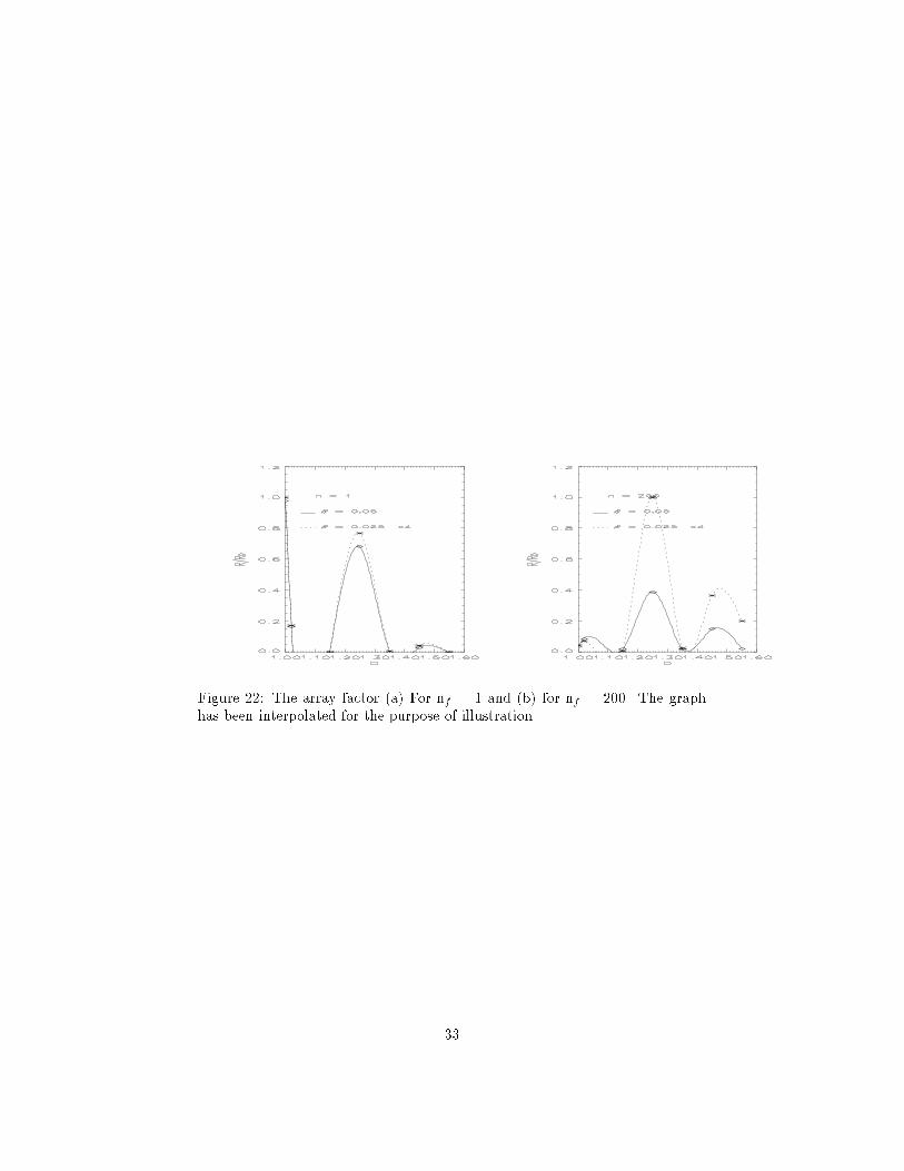
Figure 22: The array factor (a) For nf = 1 and (b) for nf = 200. The graphhas been interpolated for the purpose of illustration.

33

Figure 23: The time dependence of the radiation �elds for the fractal models.See explanation in text.

34

Figure 24: The array factor as a function of nf for � = 3:

35

Figure 25: A diagram that explains all the variables and coe�cients

36