Banks, Shadow Banking, and Fragility∗

Stephan Luck† Paul Schempp‡

September 30, 2014

This paper studies a banking model of maturity transformation in whichregulatory arbitrage induces the existence of shadow banking next to regu-lated commercial banks. We derive three main results: First, the relativesize of the shadow banking sector determines the stability of the financialsystem. If the shadow banking sector is small relative to the capacity ofsecondary markets for shadow banks’ assets, shadow banking is stable. Inturn, if the sector grows too large, it becomes fragile: an additional equi-librium emerges that is characterized by a panic-based run in the shadowbanking sector. Second, if regulated commercial banks themselves operateshadow banks, the parameter space in which a run on shadow banks mayoccur is reduced. However, once the threat of a crisis reappears, a crisis inthe shadow banking sector spreads to the commercial banking sector. Third,in the presence of regulatory arbitrage, a safety net for banks may fail toprevent a banking crisis. Moreover, the safety net may be tested and mayeventually become costly for the regulator.

JEL: G21, G23, G28

∗We are very thankful for Martin Hellwig’s extensive advice and support. We explicitly thank Jean-Edouard Colliard for very helpful comments. Moreover, we also thank Tobias Adrian, Markus Brun-nermeier, Brian Cooper, Christian Hellwig, Sebastian Pfeil, Jean-Charles Rochet, Eva Schliephake,and Ansgar Walther. This paper was awarded the Young Economist Prize at the 1st ECB Forumon Central Banking 2014 in Sintra, Portugal. Financial support by the Alexander von HumboldtFoundation and the Max Planck Society is gratefully acknowledged.

†stephan.luck@princeton.edu‡schempp@coll.mpg.de

1. Introduction

This paper contributes to the theoretical understanding of how shadow banking activities

can set the stage for a financial crisis. Maturity and liquidity mismatch in unregulated

financial intermediation – often described as shadow banking – were a key ingredient to

the 2007-09 financial crisis (Brunnermeier, 2009; FCIC, 2011). Prior to the crisis, the

shadow banking sector was largely involved in financing long-term real investments such

as housing. With an increase in delinquency rates of subprime mortgages, uncertainty

about the performance of returns of those investments emerged. This led to various

kinds of run-like events in the shadow banking sector, including the collapse of the

market for asset-backed commercial papers (ABCP) (Kacperczyk and Schnabl, 2009;

Covitz et al., 2013), the counterparty runs on Bear Stearns and Lehman Brothers in tri-

party repo (Copeland et al., 2011; Krishnamurthy et al., 2014), and the large-scale run

on the money market fund industry in the aftermath of the Lehman failure (Kacperczyk

and Schnabl, 2013; Schmidt et al., 2014). The turmoil in the shadow banking sector

ultimately translated into broader financial-sector turmoil in which several commercial

banks were on the brink of failure. Ultimately, governments and central banks had to

intervene on a large scale.

We develop a model in which shadow banking emerges alongside commercial banking

in order to circumvent financial regulation. We show that if the shadow banking sector

grows too large, fragility arises in the sense that panic-based runs may occur. The size

of the shadow banking sector is crucial because it determines the volume of assets being

sold on the secondary market in case of a run. We assume that arbitrage capital in

this market is limited. Therefore, if the shadow banking sector is too large relative

to available arbitrage capital, fire-sale prices are depressed due to cash-in-the-market

pricing, and self-fulfilling runs become possible. Moreover, if shadow banking activities

are intertwined with activities of commercial banks, a crisis in the shadow banking sector

may also trigger a crisis in the regulated banking sector. Eventually, the efficacy of

existing safety nets for regulated banks may be undermined. By considering regulatory

arbitrage, our model challenges the view that a credible deposit insurance may eliminate

adverse run equilibria in model with maturity transformation at no cost.

The term “shadow banking” was coined during the 2007-09 financial crisis in order to

describe financial intermediation activities that were unknown to a broader public prior

to the crisis.1 However, the term is imprecise and ambiguous, and its definition varies

1The expression was first used by Paul McCulley at the Jackson Hole Symposium in Wyoming, who

described shadow banking as “the whole alphabet soup of levered up non-bank investment conduits,

vehicles, and structures”(McCulley, 2007).

1

substantially even within the academic debate. Among the most prominent definitions

are the ones by Pozsar et al. (2013), by the Financial Stability Board (FSB, 2013), and by

Claessens and Ratnovski (2014).2 Building on these definitions, we use the term “shadow

banking” to describe banking activities (risk, maturity, and liquidity transformation)

that take place outside the regulatory perimeter of banking and do not have direct

access to public backstops, but may require backstops to operate.

Prior to the crisis, shadow banking had evolved as a popular alternative to commercial

banking in order to finance long-term real investments via short-term borrowing. E.g.,

asset-backed securities (ABS) were financed through asset-backed commercial papers

(ABCP). While the shadow banking sector had a stable record prior to the crisis, its

activities expanded rapidly in the years up to the crisis (see, e.g., FCIC, 2011; FSB,

2013; Claessens et al., 2012).3

The 2007-09 financial crisis began when an increase in delinquency rates of subprime

mortgages induced uncertainty about the performance of ABS. In August 2007, BNP

Paribas suspended convertibility of three of its funds that were exposed to risk of sub-

prime mortgages bundled in ABS, and there was a sharp contraction of short-term

funding of off-balance sheet conduits such as ABCP conduits and structured investment

vehicles (SIVs) that financed their ABS holdings by issuing ABCP and medium-term

notes (Kacperczyk and Schnabl, 2009). The empirical evidence suggests that this con-

traction resembled the essential features of a run-like event or a rollover freeze in the

ABCP market (see Covitz et al., 2013). Due to the breakdown of the ABCP market and

due to continuing bad news from the housing market, the institutions that produced

ABS got into trouble. This culminated in the counterparty runs on Bear Stearns in

March 2008 in tri-party repo, and finally in the collapse of Lehman Brothers in Septem-

ber 2008.4 The failure of Lehman Brothers caused further turmoil, including “Reserve

2Pozsar et al. (2013) define shadow banking as “credit, maturity, and liquidity transformation without

direct and explicit access to public sources of liquidity or credit backstops”. The FSB (2013) describes

shadow banking as “credit intermediation involving entities and activities (fully or partially) outside

the regular banking system”. Finally, Claessens and Ratnovski (2014) propose the label “shadow

banking” for “all financial activities, except traditional banking, which require a private or public

backstop to operate”. All approaches describe shadow banking as financial activities that are similar

to those of traditional banks. While the FSB emphasizes regulatory aspects, the other two address

the access to or the need for backstops. Our definition borrows from all three and tries to combine

the different aspects.3The only MMF that ever broke the buck before Lehman’s default was the “Community Bankers Money

Fund” (see Kacperczyk and Schnabl (2013)). Shadow banking activities had been evolving since the

1970s and experienced a growth boost in the 1990s when MMFs expanded their investments from

government and corporate bonds towards ABS also.4In the direct aftermath of the crisis, the academic debate had – due to the availability of data –

2

Primary Fund” breaking the buck, thus finally triggering a full-blown run on the money

market fund industry (Kacperczyk and Schnabl, 2013; Schmidt et al., 2014). Our model

contributes to the theoretical understanding for why sharp contraction in short-term

funding may occur in the shadow banking sector. In particular, our model offers a ra-

tionale of how regulatory arbitrage may set the stage for panic-based runs such as the

run on ABCP conduits and MMFs in the 2007-09 crises, and how such runs can also

adversely affect the regulated banking sector – even in the absence of runs on commercial

banks.

We discuss a simple banking model of maturity transformation in the tradition of

Diamond and Dybvig (1983) and Qi (1994) in order to illustrate how shadow banking

can sow the seeds of a financial crisis. In our model, commercial banks’ liabilities are

covered by a deposit insurance. Because this might induce moral hazard on the part

of the banks, they are subject to regulation, which induces regulatory costs for the

banks. The shadow banking sector competes with commercial banks in offering maturity

transformation services to investors. In contrast to commercial banks, shadow banking

activities are neither covered by the safety net nor burdened with regulatory costs.

Our first key result is that the relative size of the shadow banking sector determines

its stability. If the short-term financing of shadow banks breaks down, they are forced

to sell their securitized assets on a secondary market. The liquidity in this market is

limited by the budget of arbitrageurs. If the size of the shadow banking sector is small

relative to the capacity of this secondary market, shadow banks can sell their assets at

face value in case of a run. Because they can raise a sufficient amount of liquidity in

this way, a run does not constitute an equilibrium. However, if the shadow banking

sector is too large, the arbitrageurs’ budget does not suffice to buy all assets at face

value. Instead, cash-in-the-market pricing a la Allen and Gale (1994) leads to depressed

fire-sale prices in case of a run. Because shadow banks cannot raise a sufficient amount

of liquidity, self-fulfilling runs constitute an equilibrium. Depressed fire-sale prices are

reminiscent of theories on the limits to arbitrage (see, e.g., Shleifer and Vishny, 1997,

2011) and give rise to multiple equilibria in our model.

As a second key result we find that if commercial banks themselves operate shadow

banks, a larger size of the shadow banking sector is sustainable. In this case, the shadow

banking sector indirectly benefits from the safety net for commercial banks. Because of

largely focused on the run on repo (Gorton and Metrick, 2012). Copeland et al. (2011) as well as

Krishnamurthy et al. (2014) point out that the repo market experienced a margin spiral in the sense

of Brunnermeier and Pedersen (2009), but did not necessarily experience a run. The counterparty

runs on Bear Stearns in tri-party repo programs in March 2008 and the run on Lehman Brother in

September 2008 are exceptions.

3

this safety net, bank depositors never panic and banks thus have additional liquid funds

to support their shadow banks. This enlarges the parameter space for which shadow

banking is stable. However, once the threat of a crisis reappears, a crisis in the shadow

banking sector also harms the sector of regulated commercial banking.

Finally, the third important result is that a safety net for banks may not only be

unable to prevent a banking crisis in the presence of regulatory arbitrage. In fact,

it may become tested and costly for the regulator (or taxpayer). If banks and shadow

banking are separated, runs only occur in the shadow banking sector, while the regulated

commercial banking sector is unaffected. If they are intertwined, a crisis in the shadow

banking sector translates into a system-wide crisis and ultimately the safety net becomes

tested, and eventually costly, for its provider. This is at odds with the view that safety

nets such as a deposit insurance are an effective measure to prevent panic-based banking

crises. In traditional banking models of maturity transformation, such as Diamond

and Dybvig (1983) and Qi (1994), credible deposit insurance can break the strategic

complementarity of investors and eliminate adverse run equilibria at no costs, as it is

never tested. The efficacy of such safety nets was widely agreed upon until recently;

see, e.g., Gorton (2012) on “creating the quiet period”. We show that this may not be

the case when regulatory arbitrage is possible. Regulatory arbitrage may undermine the

efficacy of safety nets.

For most parts of this paper we treat the shadow banking sector as consisting of one

vertically integrated institution. However, we show that our model can be extended such

that its structure is closer to the actual shadow banking sector in the US prior to the

crisis, see also Figure 5. We mostly follow and simplify the descriptions by (Pozsar et

al., 2013) and show that all results hold when we consider a shadow banking sector that

consists of investment banks (broker dealers), ABCP conduits such as special investment

vehicles (SIVs) and money market mutual funds (MMFs) instead of single shadow banks.

This also allows us to derive separate conditions for runs from investors on MMFs and

for runs from MMFs on ABCP conduits.

The main contribution of this paper is to show how regulatory arbitrage-induced

shadow banking can contribute to the evolution of financial crises. We illustrate how

shadow banking activities undermine the effectiveness of a safety net that is installed to

prevent self-fulfilling bank runs. Moreover, we show how shadow banking may make the

safety net costly for the regulator in case of a crisis. We argue that the understanding

of how shadow banking activities contribute to the evolution of systemic risk is not only

key to understanding the recent financial crisis. Our results indicate that circumvention

of regulation can generally have severe adverse consequences on financial stability. We

4

argue that it is an essential part of any analysis of the efficacy of regulatory interventions

to consider the extent of possible regulatory arbitrage. Thus, this paper is not only

concerned with the 07-09 crisis but attempts to make more general point on the dangers

associated with regulatory arbitrage. This may be of importance for those economies in

which shadow banking is booming such as currently in China (see Awrey, 2015; Dang

et al., 2014).

While the simple nature of our model keeps the analysis tractable, we exclude certain

features that might be considered relevant. In our view, the most important ones are the

following two: First, in our model, a financial crisis is a purely self-fulfilling phenomenon.

We do not claim that the turmoils in summer 2007 were a pure liquidity problem. Clearly,

ABCP conduits had severe solvency problems as a consequence of increased delinquency

rates. However, this paper is an attempt to demonstrate how the structure of the

financial system can set the stage for a severe fragility: because of maturity mismatch

in a large shadow banking sector without an explicit safety net, small shocks can lead to

large repercussions. Second, by focusing on regulatory arbitrage as the sole reason for

the existence of shadow banking, we ignore potential positive welfare effects of shadow

banking and securitization. There are several other rationales for why shadow banking

exists: securitization can be an effective instrument to share macroeconomic interest

rate risk (Hellwig, 1994) or to cater to the demand for safe debt (Gennaioli et al., 2013);

it can make assets marketable by overcoming adverse selection problems (Gorton and

Pennacchi, 1990, 1995; Dang et al., 2013); and it can increase the efficiency of bankruptcy

processes (Gorton and Souleles, 2006). In contrast, we focus on the regulatory arbitrage

hypothesis which has received considerable support by the empirical findings of Acharya

et al. (2013). Therefore, it is important to keep in mind that whenever we speak of

shadow banking and its consequences for financial stability, we mainly address shadow

banking that originates from regulatory arbitrage. However, the fragility that we find

in our model may arguably also exists in a different context.

There is a fast-growing literature on theoretical aspects of shadow banking. Our

modeling approach is related to the paper by Martin et al. (2014). However, their

focus lies the run on repo and on the differences between bilateral and tri-party repo

in determining the stability of single financial institutions. In turn, we focus on ABCP

and system-wide crises. The paper by Bolton et al. (2011) is the first contribution to

provide an origination and distribution model of banking with multiple equilibria in

which adverse selection is contagious over time. Gennaioli et al. (2013) provide a model

in which the demand for safe debt drives securitization. In their framework, fragility in

the shadow banking sector arises when tail-risk is neglected.

5

Other contributions that deal with shadow banking are Ordonez (2013), Goodhart et

al. (2012, 2013), and Plantin (2014). Ordonez focuses on potential moral hazard on the

part of banks. In his model, shadow banking is potentially welfare-enhancing as it allows

to circumvent imperfect regulation. However, it is only stable if shadow banks value their

reputation and thus behave diligently; it becomes fragile otherwise. The emphasis of

Goodhart et al. lies on incorporating shadow banking into a general equilibrium model.

Plantin studies the optimal prudential capital regulation when regulatory arbitrage is

possible. In contrast to all three, we focus on the destabilizing effects of shadow banking

in the sense that it gives rise to run equilibria.

This paper proceeds as follows: In Section 2, we illustrate the baseline model of

maturity transformation. In Section 3, we extend the model by a shadow banking sector

and analyze under which conditions fragility arises. In Section 4, we show how the

results change when commercial banks themselves operate shadow banks. Finally, we

analyze different types of runs in the shadow banking sector in Section 5, and conclude

in Section 6.

2. A Model of Intergenerational Banking

Our baseline model is an overlapping-generation version of the model of maturity trans-

formation by Diamond and Dybvig (1983) which was first introduced by Qi (1994).

There is an economy that goes through an infinite number of time periods t ∈ Z.

There exists a single good that can be used for consumption as well as investment. In

each period t, a new generation of investors is born, consisting of a unit mass of agents.

Each investor is born with an endowment of one unit of the good, and her lifetime is

three periods: (t, t+ 1, t+ 2). Upon birth, all investors are identical, but in period t+ 1,

their type is privately revealed: With a probability of π, an investor is impatient and her

utility is given by u(ct+1). With a probability of 1 − π, the investor is patient and her

utility is given by u(ct+2). Assume that the function u(·) is strictly increasing, strictly

concave, twice continuously differentiable, and satisfies the following Inada conditions:

u′(0) =∞, and u′(∞) = 0.

In each period t, there are two different assets (investment technologies): a short

asset (storage technology), and a long asset (production technology). The short asset

transforms one unit of the good at time t into one unit of the good at t+1, thus effectively

storing the good. The long asset is represented by a continuum of investment projects.

An investment project is a metaphor for an agent who is endowed with a project (e.g.,

an entrepreneur with a production technology or a consumer who desires to finance a

6

house), but has no funds she can invest.

There is no aggregate, but only idiosyncratic return risk: each investment project

requires one unit of investment in t and yields a stochastic return of Ri units in t +

2. The return Ri is the realization of an independently and identically distributed

random variable R, characterized by a probability distribution F . F is continuous and

strictly increasing on some interval [R,R] ⊂ R+, with E[Ri] = R > 1. We assume that

the realization of an investment project’s long-term return, Ri, is privately revealed to

whoever finances the project.

The idiosyncratic return risk of the long asset implies that financial intermediaries

dominate a financial markets solution in terms of welfare because of adverse selection

in the financial market.5 In turn, unlike participants of a financial market, a financial

intermediary will not be subject to these problems as he is able to diversify and create

assets that are not subject to asymmetric information.

Finally, an investment project may be physically liquidated prematurely in t + 1,

yielding a liquidation return of `Ri/R, where ` ∈ (0, 1/R). The liquidation return

of a project thus depends on the project’s stochastic long-term return. The average

liquidation return of a project is equal to `.

Intergenerational Banking

In the following, we describe the mechanics of intergenerational banking and derive

steady state equilibria, closely following Qi (1994). We assume that there is a banking

sector operating in the economy, consisting of identical infinitely lived banks that take

deposits and make investments. It is assumed that the law of large numbers applies at

the bank level, i.e., a bank neither faces uncertainty regarding the fraction of impatient

investors nor regarding the aggregate return of the long asset.

In each period t ∈ Z, banks receive new deposits Dt. They sign a demand-deposit

contract with investors which specifies a short and a long interest rate. Per unit of

deposit, an investor is allowed either to withdraw rt,1 units after one period, or rt,2 units

after two periods. In period t, banks yield the returns from the last period’s investment

in storage, St−1, and the returns from investment in the production technology in the

second but last period, It−2. They can use these funds to pay out withdrawing investors

and to make new investment in the production and in the storage technology.

We are interested in steady states of this intergenerational banking. A steady state is

5Because asset quality is not observable, there is only one market price. Impatient consumers with

high-return assets have an incentive to liquidate them instead of selling them, and patient consumers

with low-return assets have an incentive to sell. This drives the market price below average return

and inhibits the implementation of the first-best.

7

given by a collection of payoffs, i.e., a short and a long interest rate, (r1, r2), a deposit

decision D, and an investment decisions I and S. We are only interested in those steady

states in which investors deposit all their funds in the banks, D = 1, and the total

investment in the storage and production technology does not exceed new deposits, i.e.,

S + I ≤ D.6 This yields the investment constraint

S + I ≤ 1. (1)

Moreover, we restrict attention to those steady states in which only impatient consumers

withdraw early. We will show later that these withdrawal decisions as well as the deposit

decision are actually optimal choices in a steady state equilibrium. In such a steady

state, banks have to pay πr1 units to impatient investors and (1− π)r2 units to patient

consumers in every period. Since payoffs and investments are limited by returns and

new deposits, the following resource constraint must hold:

πr1 + (1− π)r2 + S + I ≤ RI + S + 1. (2)

This constraint can be simplified to obtain a simple feasibility condition for steady-state

payoffs:

Definition 1 (Steady-state Payoff). A steady-state payoff (r1, r2) is budget feasible if

πr1 + (1− π)r2 ≤ (R− 1)I + 1. (3)

In a next step, we want to select the optimal steady state among the set of budget

feasible steady states. Our objective is to choose the steady state that maximizes the

welfare of a representative generation of investors, or equivalently, the expected utility

of one representative investor. We can partition this analysis by deriving the optimal

investment behavior of banks in a first step, and then addressing the optimal interest

rates. We see that the budget constraint (3) is not influenced by S. Thus, the banks’

optimal investment behavior follows directly:

Lemma 1 (Optimal Investment). The optimal investment behavior of banks is given by

I = 1 and S = 0, i.e., there is no investment in storage. The budget constraint reduces

to

πr1 + (1− π)r2 ≤ R. (4)

6Steady states with S+I > D also exists, but in those equilibria, banks have some wealth which is kept

constant over time, the net returns of which are payed out to investors each period. This scenario

does not appear particularly plausible or interesting.

8

The intergenerational feature of banking implies that storage is not needed for the

optimal provision of liquidity. Any investment in storage would be inefficient and would

hence imply a deterioration.

We can now derive the optimal steady-state payoffs (r1, r2), i.e., the optimal division

between long and short interest rate. It is straightforward to see that the first-best

steady-state payoff is given by perfect consumption smoothing, (rFB1 , rFB2 ) = (R,R).

However, the first-best cannot be implemented as it is not incentive compatible. The

incentive-compatibility and participation constraints are given by

r1 ≤ r2, (5)

r21 ≤ r2, (6)

and r2 ≥ R. (7)

Constraint (5) ensures that patient investors wait until the last period of their life-

time instead of withdrawing early and storing their funds. Constraint (6) ensures that

patient investors do not withdraw early and re-deposit their funds. By this type of

re-investment, investors can earn the short interest rate twice. As long as net returns

are positive, the latter condition is stronger, implying that the yield curve must not

be decreasing. Finally, constraint (7) ensures that investors do not engage in private

investment and side-trading. In fact, this condition is the upper bound to the side-

trading constraint. The adverse selection problem induced by the idiosyncratic return

risk relaxed this constraint, but the constraint will turn out not to be binding anyhow.

Obviously, constraint (6) is violated in the first-best, inducing patient investors to

withdraw early and to deposit their funds in the banks a second time. In the second-

best, constraints (4) and (6) are binding, resulting in a flat yield curve, r2 = r21. Following

Equation (4), the interest rate is such that

πr1 + (1− π)r21 = R. (8)

Proposition 1 (Qi 1994). In the second-best steady state, the intergenerational banking

sector collects the complete endowment, D = 1, and exclusively invests in the long-asset,

I = 1. In exchange, banks offer demand-deposit contracts with a one-period interest rate

given by

r∗1 =

√π2 + 4(1− π)R− π

2(1− π), (9)

and a two-period interest rate given by

r∗2 = r∗12. (10)

9

It holds that r∗2 > R > r∗1 > 1. Unlike in the Diamond and Dybvig (1983) model, the

first-best and the second-best do not coincide. The intergenerational structure introduces

the new IC constraint that the long interest rate must be sufficiently larger than the short

one in order to keep patient investors from withdrawal and reinvestment.7

Steady-State Equilibrium

Until now, we have not formally specified the game in a game-theoretic sense. Consider

the infinite game where in each period t ∈ Z, investors born in period t decide whether to

deposit, and investors born in t− 1 decide whether to withdraw or to wait for one more

period. We do not engage in a full game-theoretic analysis. In particular, we do not

characterize all equilibria of this game, but only focus on the equilibrium characterized

by the above steady state, and analyze potential deviations. Banks are assumed to

behave mechanically according to this steady state.

Lemma 2. The second-best steady state constitutes an equilibrium of the infinite game.

If all investors deposit their funds in the banks, and if only impatient consumers with-

draw early, it is in fact individually optimal for each investor to do the same. The

second-best problem already incorporates the incentive compatibility constraints as well

as the participation constraint. Patient investors have no incentive to withdraw early,

given that all other patient investors behave in the same way and given that new in-

vestors deposit in the bank. Nor do investors have an incentive to invest privately in

the production or storage technology, as the bank offers a weakly higher long-run return

that R.

Fragility

We will now study the stability of intergenerational banking in the absence of a deposit

insurance. Models of maturity transformation such as Diamond and Dybvig (1983) and

Qi (1994) may exhibit multiple equilibria in their subgames. Strategic complementarity

between the investors may give rise to equilibria in which all investors withdraw early,

i.e., bank run equilibria.

In the following, we analyze the subgame starting in period t under the assumption

that behavior until date t − 1 is as in the second-best steady-state equilibrium. We

derive the condition under which banks might experience a run by investors, i.e., the

condition for the existence of a run equilibrium in the period-t subgame. In the case

7However, the intergenerational structure also relaxes the feasibility constraint. Although the yield

curve is allowed to be decreasing in the model of Diamond and Dybvig (1983), the second-best of

intergenerational banking dominates the first-best of Diamond and Dybvig (1983) for a large set of

utility functions because banks do not have to rely on inefficient storage.

10

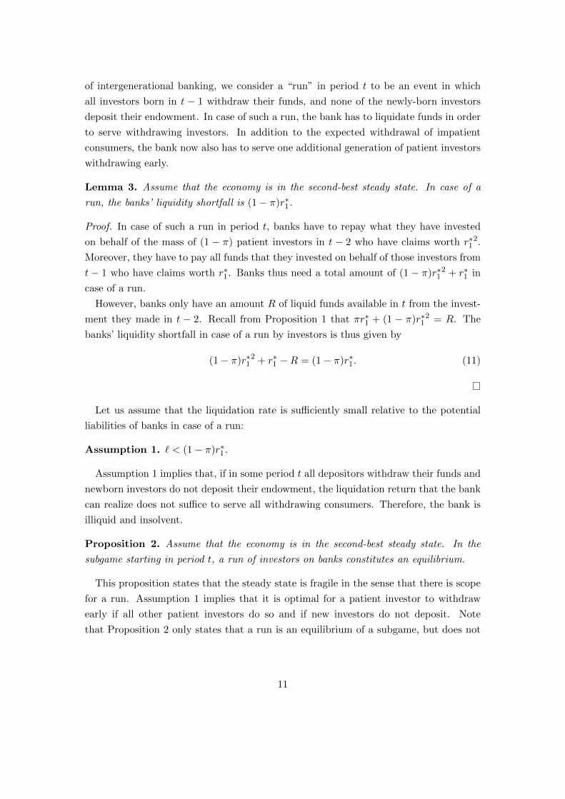
of intergenerational banking, we consider a “run” in period t to be an event in which

all investors born in t − 1 withdraw their funds, and none of the newly-born investors

deposit their endowment. In case of such a run, the bank has to liquidate funds in order

to serve withdrawing investors. In addition to the expected withdrawal of impatient

consumers, the bank now also has to serve one additional generation of patient investors

withdrawing early.

Lemma 3. Assume that the economy is in the second-best steady state. In case of a

run, the banks’ liquidity shortfall is (1− π)r∗1.

Proof. In case of such a run in period t, banks have to repay what they have invested

on behalf of the mass of (1 − π) patient investors in t − 2 who have claims worth r∗12.

Moreover, they have to pay all funds that they invested on behalf of those investors from

t − 1 who have claims worth r∗1. Banks thus need a total amount of (1 − π)r∗12 + r∗1 in

case of a run.

However, banks only have an amount R of liquid funds available in t from the invest-

ment they made in t − 2. Recall from Proposition 1 that πr∗1 + (1 − π)r∗12 = R. The

banks’ liquidity shortfall in case of a run by investors is thus given by

(1− π)r∗12 + r∗1 −R = (1− π)r∗1. (11)

Let us assume that the liquidation rate is sufficiently small relative to the potential

liabilities of banks in case of a run:

Assumption 1. ` < (1− π)r∗1.

Assumption 1 implies that, if in some period t all depositors withdraw their funds and

newborn investors do not deposit their endowment, the liquidation return that the bank

can realize does not suffice to serve all withdrawing consumers. Therefore, the bank is

illiquid and insolvent.

Proposition 2. Assume that the economy is in the second-best steady state. In the

subgame starting in period t, a run of investors on banks constitutes an equilibrium.

This proposition states that the steady state is fragile in the sense that there is scope

for a run. Assumption 1 implies that it is optimal for a patient investor to withdraw

early if all other patient investors do so and if new investors do not deposit. Note

that Proposition 2 only states that a run is an equilibrium of a subgame, but does not

11

say anything about equilibria of the whole game. However, our emphasis lies on the

stability/fragility of the steady-state equilibrium.

An important insight from Diamond and Dybvig (1983) and Qi (1994) is that a credible

deposit insurance may actually eliminate the adverse equilibrium at no cost. If the

insurance is credible, it eliminates the strategic complementarity and is thus never tested.

In fact, this is also true in the setup described above. Assume that there is a regulator

that can cover the liquidity shortfall in any contingency, including a full-blown bank run.

In the context of our model, this amounts to assuming that the regulator has funds of

(1 − π)r∗1 − ` at its disposal in any period. Whenever patient investors are guaranteed

an amount r∗1 by the regulator, they do not have an incentive to withdraw early.8 In

contrast, this does not hold in the presence of regulatory arbitrage, as we will show in

the following sections.

3. Banks and Shadow Banks

We now extend the model described above by three elements: First, we make the as-

sumption that commercial banks are covered by a safety net, but are also subject to

regulation and therefore have to bear regulatory costs. Second, there are unregulated

shadow banks that compete with banks by also offering maturity transformation ser-

vices. Investors can choose whether to deposit their funds in a bank or in the shadow

bank. Depositing in the shadow bank is associated with some opportunity cost that

varies across investors. Third, there is a secondary market in which shadow banks can

sell their assets to arbitrageurs. The amount of liquidity in this market is assumed to

be exogenous.

In the following, we describe the extended setup in detail and derive the steady-

state equilibrium, before analyzing whether the economy is stable or whether it features

multiple equilibria and panic-based runs may occur.

Commercial Banking and Regulatory Costs

From now on, we assume that commercial banks are covered by a safety net that is pro-

vided by some unspecified regulator, ruling out runs in the commercial banking sector.9

Because of this safety net, banks are not disciplined by their depositors, such that – in a

8We ignore the possibility for suspension of convertibility. Diamond and Dybvig (1983) already indicate

that suspension of convertibility is critical if there is uncertainty about the fraction of early and late

consumers. Moreover, as Qi (1994) shows, suspension of convertibility is also ineffective if withdrawing

depositors are paid out by new depositors.9The regulator is assumed to have sufficient funds to provide a safety net. Moreover, he can commit

to actually applying the safety net in case it is necessary, i.e., in case of a run.

12

richer model – moral hazard could arise. We therefore assume that banks are regulated

(e.g., they are subject to a minimum capital requirement). This is assumed to be costly

for the bank. In what follows, we will not model the moral hazard explicitly and assume

that regulatory costs are exogenous. However, in Appendix A we provide an extension

of our model in which we illustrate how moral hazard may arise from the existence of the

safety net, and why costly regulation is necessary to prevent moral hazard. The presence

of a credible deposit insurance implies that depositors have no incentive to monitor their

bank. Because banks have limited liability, this gives bankers an incentive to engage

in excessive risk-taking or to invest in assets with private benefits. This in turn calls

for regulatory interventions, e.g., in the form of minimal capital requirements which are

costly for bank managers.

We assume that banks have to pay a regulatory cost γ per unit invested in the long

asset, resulting in a gross return of R− γ. We further assume that regulatory costs are

not too high, i.e., even after subtracting the regulatory costs, the long asset is still more

attractive than storage.

Assumption 2. R > 1 + γ.

Because of the lower gross return, banks can now only offer a per-period interest rate

rb such that

πrb + (1− π)r2b = R− γ. (12)

Under this regulation, the interest rate on bank deposits is explicitly given by

rb =

√π2 + 4(1− π)(R− γ)− π

2(1− π). (13)

The banking sector thus functions like the banking sector in the previous section. The

only difference is that banks cannot transfer the gross return R to investors, but only

the return net of regulatory cost, R− γ.

Shadow Banks

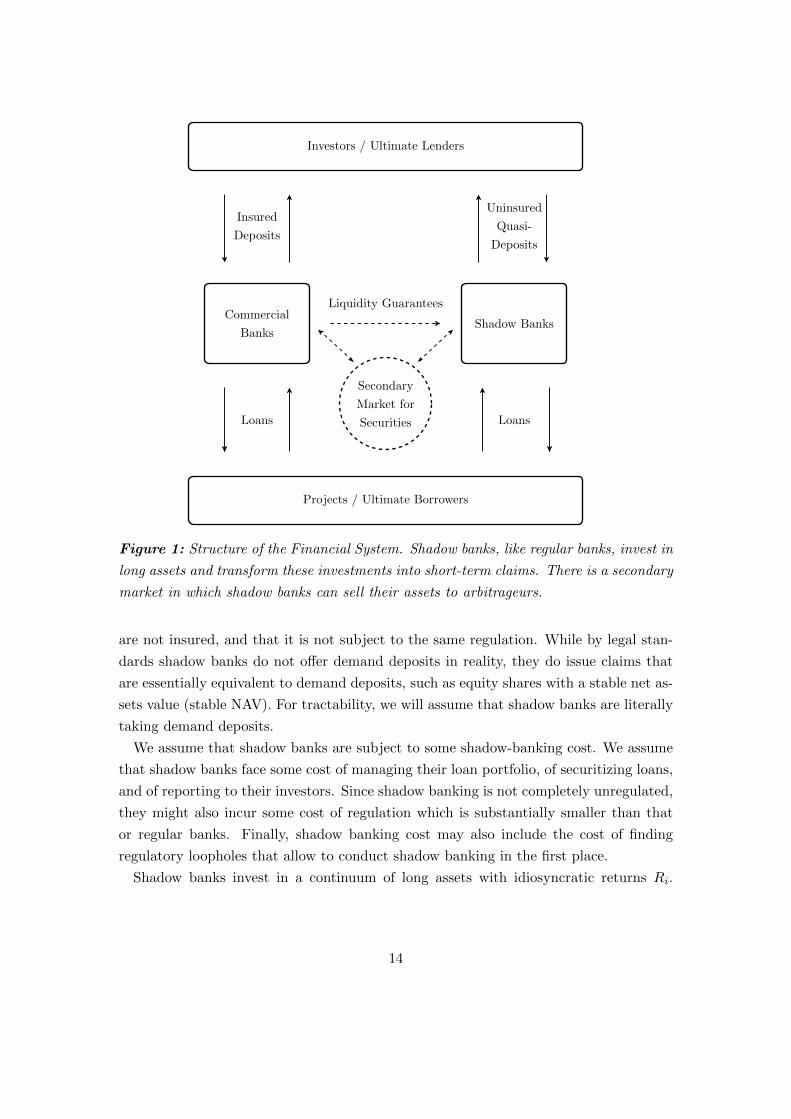
We now introduce a shadow banking sector that also offers credit, liquidity, and matu-

rity transformation to investors. We start out with very simple structure of the financial

system, see Figure 1. Shadow banks, like regular banks, invest in long assets and trans-

form these investments into short-term claims. In this section, we do not distinguish

between different actors in the shadow banking sector, but assume that there is one

representative, vertically integrated institution that we call shadow bank. This shadow

bank is essentially identical to a commercial bank, with the exception that its deposits

13

Investors / Ultimate Lenders

Projects / Ultimate Borrowers

Commercial

Banks

Insured

Deposits

Loans

Shadow Banks

Uninsured

Quasi-

Deposits

Loans

Secondary

Market for

Securities

Liquidity Guarantees

Figure 1: Structure of the Financial System. Shadow banks, like regular banks, invest in

long assets and transform these investments into short-term claims. There is a secondary

market in which shadow banks can sell their assets to arbitrageurs.

are not insured, and that it is not subject to the same regulation. While by legal stan-

dards shadow banks do not offer demand deposits in reality, they do issue claims that

are essentially equivalent to demand deposits, such as equity shares with a stable net as-

sets value (stable NAV). For tractability, we will assume that shadow banks are literally

taking demand deposits.

We assume that shadow banks are subject to some shadow-banking cost. We assume

that shadow banks face some cost of managing their loan portfolio, of securitizing loans,

and of reporting to their investors. Since shadow banking is not completely unregulated,

they might also incur some cost of regulation which is substantially smaller than that

or regular banks. Finally, shadow banking cost may also include the cost of finding

regulatory loopholes that allow to conduct shadow banking in the first place.

Shadow banks invest in a continuum of long assets with idiosyncratic returns Ri.

14

As the law of large numbers is assumed to apply, the return of their portfolio is R.

Similar to regulatory costs, shadow banking is assumed to come with a per-unit cost

of ρ. Therefore, the per-unit return of assets in the shadow banking sector is R − ρ.

Similar to the regulatory cost γ, we also assume that the shadow-banking cost is not too

high, i.e., even after subtracting the shadow-banking cost, the long asset is still more

attractive than storage:

Assumption 3. R > 1 + ρ.

Given this shadow-banking cost, shadow banks offer a per-period interest rate rsb to

investors such that

πrsb + (1− π)r2sb = R− ρ, (14)

implying a return of

rsb =

√π2 + 4(1− π)(R− ρ)− π

2(1− π). (15)

Secondary Markets and Arbitrageurs

There exists a secondary market for the shadow banks’ assets. The potential buyers on

this market are arbitrageurs who have an outside option with a risk-free return of r,

i.e., they are willing to buy the shadow banks’ assets at a price that offers them a safe

return of at least r. Arbitrageurs can be thought of as experts (pension funds, hedge

funds) that do not necessarily hold such assets in normal times, but purchase them if

they are available at some discounts and thus promise gains from arbitrage. Moreover,

we assume that arbitrageurs do not want to deposit their funds in shadow banks because

their outside option is more attractive:

Assumption 4. r > rsb.

This reservation interest rate implies that arbitrageurs’ reservation price for an asset

with a return of R− ρ is given by pa = (R− ρ)/r.

Assume that there is no market power on any side of the secondary market. Moreover,

there is a fixed amount of cash in this market. We assume that arbitrageurs have a total

budget of A, implying that cash-in-the-market pricing can occur. The equilibrium supply

and price of shadow banks’ assets on the secondary market will be derived below.

The idea behind this assumption is that not every individual or institution has the

expertise to purchase these financial products. Moreover, the equity and collateral of

these arbitrageurs is limited, so they cannot borrow and invest infinite amounts.10

10See Shleifer and Vishny (1997) for a theory on the limits to arbitrage.

15

Upon birth, investors can choose whether to deposit their endowment in a regulated

bank or in a shadow bank. Depositing at shadow bank comes at some opportunity

cost. We assume that investors are initially located at a regulated bank. Switching to a

shadow bank comes at a cost of si, where si is independently and identically distributed

according to the distribution function G. We assume that G is a continuous function

that is strictly increasing on its support R+, and that G(0) = 0. The switching cost is

assumed to enter into the investors’ utility additively separable from the consumption

utility.

This switching cost should not be taken literally. One can think of these costs as mon-

itoring or screening costs for investors that become necessary when choosing a shadow

bank (e.g., an MMF) as these are not protected by a deposit insurance (see Appendix A

for more details). For simplicity, we have assumed that all depositors have the same size.

However, we could alternatively come up with a model where investors have different

endowments (see Appendix B). It is very plausible that the ratio of switching costs to

the endowment is lower for larger investors (e.g., for corporations that need to store

liquid funds of several millions for a few days). Another interpretation is the forgone

service benefits that depositors lose when leaving commercial banks, such as payment

services and ATMs.

Investors’ Behavior

Given the interest rates of commercial banks, rb, of shadow banks, rsb, and given the

switching cost distribution G, we can pin down the size of the shadow banking sector.

Lemma 4. Assume that banks offer an interest rate rb and shadow banks offer an

interest rate of rsb, as specified above. Then there exists a unique threshold s∗ such that

an investor switches to a shadow bank if and only if si ≤ s∗. The mass of investors

depositing in the shadow banking sector is given by G(s∗). It holds that s∗ = f(γ, ρ),

where fγ > 0 and fρ < 0.

Proof. Take rb and rsb as described above. We know rb decreases in γ, and rsb decreases

ρ. Staying at a commercial bank provides an investor with an expected consumption

utility of EUb = πu(rb) + (1 − π)u(r2b ). Switching to a shadow bank is associated with

an expected consumption utility of EUsb = πu(rsb) + (1 − π)u(r2sb). Observe that EUb

decreases in γ and EUsb decreases in ρ.

An investor with switching cost si switches to the shadow banking sector if EUb <

EUsb−si. This implies that all investors with si ≤ EUsb−EUb switch to shadow banks.

We define s∗ ≡ f(γ, ρ) = EUsb(ρ)−EUb(γ). A mass G(s∗) of each generation’s investors

switches to shadow banks, and a mass 1 − G(s∗) stays at commercial banks. Because

16

u is twice continuously differentiable, it holds that ∂EUb/∂γ < 0 and ∂EUsb/∂ρ > 0.

Thus, f is a continuously differentiable function with fγ > 0 and fρ < 0.

An investor with si = s∗ is indifferent between depositing at a bank or a shadow bank.

All investors with lower switching costs choose a shadow; their mass is given by G(s∗).

The size of the shadow banking sector increases in the regulatory cost γ and decreases

in the shadow-banking cost ρ. For the case of logarithmic utility, the switching point is

given by s∗ = (2− π)γ − ρ.

We are now equipped to characterize the economy’s steady state equilibrium:

Proposition 3. In the second-best steady-state equilibrium, the intergenerational bank-

ing sector collects an amount of deposits Db = 1 − G(s∗) in each period, and invests

all funds in the long-asset, Ib = 1−G(s∗). They offer demand-deposit contracts with a

per-period interest rate of

rb =

√π2 + 4(1− π)(R− γ)− π

2(1− π). (16)

Shadow banks collect an amount of deposits Dsb = G(s∗) and exclusively invest in ABS,

Isb = 1−G(s∗). They offer a demand-deposit contracts with a per-period interest rate of

rsb =

√π2 + 4(1− π)(R− ρ)− π

2(1− π). (17)

It holds that s∗ = f(γ, ρ), where fγ > 0 and fρ < 0. There are no assets traded in the

secondary market.

Proposition 3 described the steady state in which regulated commercial banks and

shadow banks coexist. The interest rates are given by rb and rsb and depend on γ and

ρ, which determines the size of the shadow banking sector as described by Lemma 4. It

is important to notice that, in this steady-state equilibrium, no assets are being sold to

arbitrageurs on the secondary market, as there are no gains from trade.

3.1. Fragility of Shadow Banks

As in the previous section, we now study the stability of shadow banks. We analyze

the subgame starting in period t under the assumption that behavior until date t − 1

is as in the steady-state equilibrium specified in Proposition 3. We derive the condition

under which shadow banks might experience a run by investors, i.e., the condition for

the existence of a run equilibrium in the period-t subgame.

Because deposits in the shadow banking sector are not insured, a run on shadow

banks is not excluded per se. However, as will become clear below, runs only occur if

17

the shadow banking sector is too large. Generally, there are two types of runs that could

potentially take place in the adverse equilibrium of the t = 1 subgame.

In our model, a run is the event where all old investors withdraw their funds from

shadow banks, and new investors do not deposit any new funds. Whether a run on

shadow banks constitutes an equilibrium depends on whether shadow banks can raise

enough liquidity in the secondary market to serve all their obligations.

Lemma 5. Assume that the economy is in the second-best steady state. In case of a run

on shadow banks, their liquidity shortfall is given by G(s∗)(1− π)rsb.

Proof. See proof of Lemma 3. (1 − π)rsb is the relative liquidity shortfall, the amount

of missing liquidity per unit of investment in the shadow banking sector.

In order to cover this shortfall, shadow banks can either sell their investment of period

t−1 to the arbitrageurs, or they can liquidate these assets.11 We assume that liquidation

of assets will never be enough to cover the shortfall:

Assumption 5. ` < (1− π)rsb.

This assumption implies that the liquidation value is sufficiently smaller than the long-

run net return R− ρ. Similar to Assumption 1, also in the case of shadow banks, which

pay a per-period interest of rsb, liquidation cannot be used to serve investors.

In the last section, the assumption of a low liquidation value implied that (in the

absence of a deposit insurance) a run on banks can always occur. The presence of arbi-

trageurs who are willing to buy shadow banks’ assets in a secondary market implies that

the threat of a run is not necessarily omnipresent. We will show that the arbitrageurs’

valuation of these assets and, more importantly, the size of their budget determines

whether run equilibria exist.

Lemma 6. Assume that the economy is in the second-best steady state. A run on shadow

banks constitutes an equilibrium of the period-t subgame if

R− ρr

< (1− π)rsb. (18)

If the arbitrageurs’ outside option is very profitable, they are only willing to pay a

low price. If this price is lower than the relative liquidity shortfall, a run is always

11Liquidation is not essential to our model. It also goes through in case liquidation is not possible; we

can just set ` = 0.

18

self-fulfilling. Shadow banks have to sell their assets, and the resulting revenue does

not suffice to serve all investors because the arbitrageurs’ valuation and thus the market

price are too low.

From now on, we will assume that the arbitrageurs’ outside option is not too profitable,

i.e., their reservation price is sufficiently large:

Assumption 6. (R− ρ)/r ≥ (1− π)rsb.

Observe that, in case of a run shadow banks’ supply is partially inelastic as they have

to cover their complete liquidity shortfall. There are two cases to be considered: In the

first case, the arbitrageurs’ funds are sufficient to purchase all funds the shadow banks

sell at face value, while in the second case, the arbitrageurs’ budget is not sufficient and

the price is determined by cash-in-the-market pricing. Runs on shadow banks constitutes

an equilibrium only in this second case.

Proposition 4. Assume that the economy is in the second-best steady state. A run on

shadow banks constitutes an equilibrium of the period-t subgame if and only if

G(s∗) >A

(1− π)rsb≡ ξ. (19)

Proof of Proposition 4. Assume that investors collectively withdraw funds from shadow

banks and deposit no new funds in period t. It will be optimal for a single investor also

to withdraw if the shadow banks become illiquid and insolvent in t.

Recall from Lemma 5 that the liquidity shortfall of shadow banks in case of a run is

given by LS = G(s∗)(1− π)rsb. Liquidating all assets would yield G(s∗)`. According to

Assumption 5, this will always be less than the liquidity shortfall. Shadow banks will

never be able to cover the liquidity shortfall by liquidating their assets.

The relevant question is whether shadow banks can raise sufficient funds by selling

their assets to arbitrageurs. There are two conditions which are jointly necessary and

sufficient: First, the funds of arbitrageurs have to exceed the liquidity shortfall, and

second, the arbitrageurs’ valuation of shadow banks’ assets has to exceed the liquidity

shortfall. The second condition is met by assumption.

Regarding the first condition, there are two cases to be considered: In the first case, the

arbitrageurs’ funds exceed the liquidity shortfall. Because the shortfall by assumption is

lower than the valuation of arbitrageurs, their funds are sufficient to purchase all funds

the shadow banks sell at the reservation price. In the second case, the arbitrageurs’

budget is not sufficient, and the price is determined by cash-in-the-market pricing.

19

The first case is given by A ≥ (1 − π)rsbG(s∗). All assets held by shadow banks can

be sold at the arbitrageurs’ reservation price pa = (R− ρ)/r. Because the arbitrageurs’

valuation of shadow banks’ assets as well as the amount of cash in the market exceeds

the shadow banks’ potential liquidity needs, all investors could be served in case of a run.

It thus is a strictly dominant strategy for each old patient investor not to withdraw, and

for new investors to deposit new funds, and a run does not constitute an equilibrium.

The second case is given by A < (1−π)rsbG(s∗). In this case, shadow banks cannot sell

all their assets at the arbitrageurs’ reservation price. If all existing investors withdraw

and no new investors deposit, shadow banks cannot raise the required funds to fulfill

their obligations by selling their assets because the amount of assets on the secondary

market exceeds the budget of arbitrageurs. The asset price drops below the reservation

price and shadow banks are forced to sell their entire portfolio. Still, shadow banks

can only raise a total amount A of liquidity, which is insufficient to serve withdrawing

investors. It follows that, in this case, it is optimal for old and new investors to withdraw

and not to deposit, respectively. A run thus constitutes an equilibrium if and only if the

stated condition is satisfied.

The key mechanism giving rise to multiple equilibria is cash-in-the-market pricing

(see, e.g., Allen and Gale, 1994) in the secondary market for long assets. It results from

limited arbitrage capital and is related to the notion of limits to arbitrage (see, e.g.,

Shleifer and Vishny (1997)). The fact that there are not enough arbitrageurs (and that

these arbitrageurs cannot raise enough funds) to purchase all assets of the shadow banks

can induce the price of assets to fall short of pa. This implies that shadow banks may

in fact be unable to serve their obligations once they sell all their long-term securities

prematurely. This, in turn, makes it optimal for investors to run on shadow banks once

all other investors run.

In order to illustrate the role of limited availability of arbitrage capital we examine

the hypothetical fire-sale price. Cash-in-the-market pricing describes a situation where

the buyers’ budget constraint is binding and the supply is fixed. The price adjusts such

that demand balances the fixed supply. If the arbitrageurs’ budget is a binding resource

constraint, the price p is such that

pG(s∗) = A. (20)

The fire-sale price is a function of the amount of assets that are on the market in case

of a run on the shadow banking sector, which is given by the size of the shadow banking

sector G(s∗). The price is given by

20

00

pa = (R− ρ)/r

(1− π)rsb

`

p

G(s∗)ξ A/`

Stability Fragility

Unique equilibrium

Multiple equilibria

Figure 2: Fire-sale Prices. This graph depicts the potential fire-sale prices of shadow

banks’ securities. Whenever G(s∗) ≤ ξ = A/(1−π)rsb, arbitrageurs’ funds suffice to pur-

chase all assets of shadow banks at face value. In the unique equilibrium of the period-t

subgame, there are no panic-based withdrawals from shadow banks. In turn, if G(s∗) > ξ,

the funds of arbitrageurs are insufficient, and the period-t subgame has multiple equilib-

ria. If all investors withdraw from shadow banks, the price in the secondary market drops

to the red line.

p(s∗) =

(R− ρ)/r if G(s∗) ≤ ξ,

A/G(s∗) if G(s∗) ∈ (ξ, A/`] ,

` if G(s∗) > A/`.

(21)

The equilibrium fire-sale prices as a function of the size of the shadow banking sector

is illustrated in Figure 2.

Whether the period t subgame has multiple equilibria ultimately depends on the

parameters ρ and γ, as they determine the size of the shadow banking sector. This

is depicted in Figure 3. Whenever the regulatory costs γ exceed the shadow-banking

costs ρ (i.e., above the 45 degree line), the shadow banking sector has positive size

in equilibrium, i.e. G(s∗) > 0. However, as long as the shadow banking sector is

small relative to the arbitrageurs’ budget, it is stable. Only when regulatory costs γ are

21

00

R− 1

γ

R− 1 ρ

No Shadow Banking

G(s∗) = 0

Stable

Shadow Banking

0 < G(s∗) < ξ

Fragility

G(s∗) > ξ

Figure 3: Existence of Equilibria. This figure visualizes the equilibrium characteristics

of the financial system for different values of γ and ρ. For γ < ρ, shadow banking is

not made use of in equilibrium, as it is dominated by commercial banking. If γ > ρ, the

shadow banking sector has positive size. As long as the difference γ− ρ is small, shadow

banking is stable. If the difference increases, the size of the shadow banking sector also

increases and finally introduces fragility into the financial system.

sufficiently larger than shadow-banking cost ρ does the size G(s∗) of the shadow banking

sector exceed the critical threshold ξ, and shadow banking becomes fragile.

3.2. Liquidity Guarantees

So far, there has been no connection between the regulated commercial banking sector

and the shadow banking sector; both sectors compete for the investors’ funds. We now

assume that commercial banks themselves actively engage in shadow banking: They en-

gage in shadow banking through off-balance sheet subsidiaries, i.e., they operate shadow

banks as documented in Acharya et al. (2013). Our model provides a positive analysis,

the fact that banks engage in shadow banking themselves does not result from optimal

behavior in our setup. We assume that commercial banks explicitly or implicitly pro-

vide their shadow banks with liquidity guarantees. They may have strong incentives to

support their conduits in case of distress, e.g., in order to protect their reputation, see

22

Segura (2014). Moreover, we assume that commercial banks can sell their assets on the

same secondary market as shadow banks.12

As above, we assume that the commercial banks’ demand-deposit liabilities are covered

by a credible safety net. This safety net being credible implies that commercial banks

do not experience runs by investors. Patient investors who are located at a commercial

bank will thus never withdraw their funds early.

Liquidity guarantees imply that in case of a run on shadow banks, commercial banks

supply them with liquid funds. This increases the critical size up to which the shadow

banking sector is stable. However, this comes with an unfavorable side effect: Once this

critical size is exceeded and shadow banks experience a run, the crisis spreads to the

commercial banking sector and makes the safety net costly.

Proposition 5. Assume that the economy is in the second-best steady state described

in Proposition 3 and all shadow banks are granted liquidity guarantees by commercial

banks. A run of investors on shadow banks constitutes an equilibrium of the subgame

starting in period t if and only if

G(s∗) >max[A, `] + 1

(1− π)rsb + 1≡ ϑ, (22)

where s∗ = f(γ, ρ). It holds that ϑ > ξ.

Proof. In case of a run, the shadow banks’ need for liquidity is given as above by

G(s∗)(1− π)rsb.

Banks can sell their loans on the same secondary market in case of a crisis. Still, the

total endowment of arbitrageurs in this market is given by A. Therefore, either banks

and shadow banks sell their assets in the secondary market, or both types of institutions

liquidate their assets. They jointly still only raise an amount A from selling long-term

securities on the secondary market or ` units from liquidating all long assets. The

maximum amount they can raise is thus max[A, `]. On top, commercial banks also have

an additional amount 1−G(s∗) of liquid funds available since new investors still deposit

their endowment at commercial banks because of the safety net for commercial banks.

The liquidity guarantees by commercial banks can satisfy the shadow banks’ liquidity

needs in case of a run if

max[A, `] + (1−G(s∗)) ≥ G(s∗)(1− π)rsb, (23)

12It is not straightforward that banks can sell their loans on the ABS market. In case of a crisis, however,

banks might try to securitize their loan portfolio in order to sell it.

23

which is equivalent to

G(s∗) ≤ max[A, `] + 1

(1− π)rsb + 1= ϑ. (24)

If G(s∗) ≤ ϑ, the liquidity guarantees suffice to satisfy the liquidity needs in case of a

run, so a run does not constitute an equilibrium. If G(s∗) > ϑ, the liquidity guarantees

do suffice to satisfy the liquidity needs in case of a run, and a run does constitute an

equilibrium.

If commercial banks themselves operate shadow banks and provide them with liquidity

guarantees, the parameter space in which shadow banking is stable is enlarged compared

to a situation without liquidity guarantees, i.e., the critical threshold for the size of the

shadow banking sector ϑ is now larger than ξ, the threshold in the absence of liquidity

guarantees. This shift is also depicted in Figure 4. The reason for this result is that banks

have additional liquid funds, even in case of a crisis: Because of the deposit insurance,

they always receive funds from new depositors, and their patient depositors never have

an incentive to withdraw early.

00

p

G(s∗)

(R− ρ)/r

ξ

(1− π)rsb

`

A/`

Stability Fragility

Unique equilibrium

Multiple equilibria

ϑ

Figure 4: Fire-sale Prices under Liquidity Guarantees. This graph depicts the potential

fire-sale price of securities in case regulated commercial banks provide liquidity guarantees

to shadow banks. The critical size above which multiple equilibria exist moves from ξ to

ϑ.

24

In traditional banking models, policy tools like a deposit insurance eliminate self-

fulfilling adverse equilibria at no cost. This is not necessarily true in our model: once

the shadow banking sector exceeds the size ϑ, a run in the shadow banking sector

constitutes an equilibrium despite the safety net for commercial banks, and despite the

liquidity guarantees of banks. Shadow banks – by circumventing the existing regulation

– place themselves outside the safety net and are thus prone to runs. If the regulated

commercial banks offer liquidity guarantees, a crisis in the shadow banking sector also

spreads to the regulated banking sector. Ultimately, self-fulfilling adverse equilibria are

not necessarily eliminated by the safety net and may become costly.

Corollary 1. Assume that G(s∗) > ϑ, and assume banks provide liquidity guarantees to

shadow banks. In case of a run in the shadow banking sector, the safety net for regulated

commercial banks is tested and the regulator must inject an amount

G(s∗)(1− π)rsb −max[A, `] > 0. (25)

Proof. This corollary follows directly from the proof of Proposition 5. G(s∗)(1 − π)rsb

denotes the liquidity need of shadow banks in case of a run, and max[A, `] denotes

the amount that shadow banks can raise by selling or liquidating their assets. While

commercial banks may cover part of the shadow banks’ liquidity short-fall by fulfilling

their liquidity guarantees, this amount also has to be compensated by the regulator

because otherwise banks cannot serve their depositors in the future.

If the regulated commercial banking and the shadow banking sector are intertwined, a

crisis may not be limited to the shadow banking sector, but also spread to the commercial

banks, thus testing the safety net. Ultimately, the regulator has to step in and cover

the commercial banks’ liabilities. Therefore, the model challenges the view that policy

measures like a deposit insurance necessarily are an efficient mechanism for preventing

self-fulfilling crises. Historically, safety nets such as a deposit insurance schemes were

perceived as an effective measure to prevent panic-based banking crises. The view is

supported by traditional banking models of maturity transformation such as Diamond

and Dybvig (1983) and Qi (1994). In the classic models of self-fulfilling bank runs, a

credible deposit insurance can break the strategic complementarity in the withdrawal

decision of bank customers at no cost. We show that this may not be the case when

regulatory arbitrage is possible and regulated and unregulated banking activities are

intertwined.

25

4. MMFs, ABCP Conduits, and SPV

In the last section we presented a model in which the shadow banking sector consisted

of one vertically integrated, representative shadow bank. We will now consider a shadow

banking sector that offers credit, liquidity, and maturity transformation to investors

through vertically separated institutions. This structure of the shadow banking sector

(compare Figure 5) is exogenous in our model. It is empirically motivated; we selectively

follow and simplify the descriptions by Pozsar et al. (2013). Altogether, the actors of the

shadow banking system invest in long assets and transform these investments into short-

term claims. However, we distinguish between different actors in the shadow banking

sector.

In our setup, shadow banking consists of special purpose vehicles (SPVs), ABCP

conduits, and money market mutual funds (MMFs). Investment banks securitize assets

such as loans (i.e., the long assets in our model) via SPVs, thereby transforming them

into asset-backed securities (ABS). Through diversified investments, they eliminate the

idiosyncratic risk of loans and conduct risk transformation. Note that SPVs typically do

not lend to firms or consumers directly, but rather purchase loans from loan originators

such as mortgage agencies or commercial banks.

SPVs buy long assets with idiosyncratic returns, transform them into ABS, and sell

them to ABCP conduits. The empirically motivated narrative is that investment banks

use SPVs to purchase loans from loan originators such as mortgage brokers or commer-

cial banks. These SPVs bundle the claims into securitized loans (ABS), successfully

diversifying the idiosyncratic return risk. Securitization makes the long assets tradable

by eliminating the adverse selection problem that is associated with idiosyncratic return

risk. For simplicity, we assume that the shadow-banking cost ρ occurs at this stage.

Thus, the ABS that are sold by SPVs have a return of R− ρ.

ABCP conduits purchase these securitized assets with long maturities (ABS) and

finance their business by issuing short-term claims that they sell to MMFs. To put

it more technically, ABCP conduits (such as structured investment vehicles (SIVs))

purchase ABS and finance themselves through asset-backed commercial papers (ABCPs),

which they sell to MMFs.13 ABCP conduits hence conduct maturity transformation.

Maturity transformation is the central element and the key service of banking in our

model, and it is the main source of fragility.

For investors, MMFs are the door to the shadow banking sector as they transform

short-term debt (such as ABCP) into claims that are essentially equivalent to demand

13ABCP conduits also use other securities to finance their activities, such as medium term notes. For

simplicity, we focus on ABCPs.

26

Investors / Ultimate Lenders

Projects / Ultimate Borrowers

Commercial

Banks

Insured

Deposits

Loans

MMF

ABCP conduit

SPV

Quasi-

deposits

ABCP

ABS

Loans

Secondary

Market for

Securities

Liquidity Guarantees

Service division in the

shadow banking sector

Liquidity

transformation

Maturity

transformation

Risk transformation

(securitization)

Loan origination by

commercial banks

or mortgage brokers

Figure 5: Detailed Structure of Shadow Banking. The structure of the shadow banking

sector is mostly exogenous in our model; we selectively follow and simplify the descrip-

tions by Pozsar et al. (2013). Shadow banking consists of special purpose vehicle (SPVs),

ABCP conduits such as structured investment vehicles (SIVs), and money market mu-

tual funds (MMFs). SPVs transform assets into asset-backed securities (ABS) in order

to make them tradable, i.e., they conduct risk and liquidity transformation (securitiza-

tion). ABS have a long maturity; they are bought by ABCP conduits. ABCP conduits,

in turn, use short-term debt to finance these long-term assets; they sell asset-backed com-

mercial papers (ABCP) to MMFs, i.e., they conduct maturity transformation. MMFs

are the door to the shadow banking sector: They offer deposit-like claims to investors,

such as shares with a stable net assets value (NAV), thus conducting another form of

liquidity transformation. Finally, there is a secondary market in which ABS can be sold

to arbitrageurs.

27

deposits, such as equity shares with a stable net assets value (stable NAV). MMFs thus

conduct liquidity transformation. Again, we will assume that MMFs are literally taking

demand deposits.

At the heart of the shadow banking sector is the maturity transformation by ABCP

conduits. ABCP conduits purchase securitized assets (ABS) from investment banks’

SPVs. As described above, these assets have a return of R − ρ and a maturity of two

periods. ABCP conduits can finance themselves by borrowing from MMFs via ABCPs.

Moreover, they can also sell ABS to arbitrageurs in the secondary market as specified

above. ABCP conduits may be legally independent entities, but they are largely founded

and run by regulated banks in order to engage in unregulated off-balance sheet maturity

transformation (Acharya et al., 2013). Because such maturity transformation is very

fragile, banks stabilize their conduits by providing them with liquidity guarantees. In

this section, we assume that ABCP conduits are fully insured through such liquidity

guarantees.

Investors can access the services of the shadow banking sector via MMFs, which are

assumed to intermediate between investors and ABCP conduits.14 MMFs offer demand-

deposit contracts to investors while purchasing short-term claims on ABCP conduits.15

MMFs offer a per-period interest rate rmmf to investors and purchase ABCP (short-term

debt) with a per-period return rabcp. Competition among MMFs and among ABCP

conduits implies that rmmf = rabcp = rsb. Investors face the same situation as described

in the last section, and the size of the shadow banking sector is again given by G(s∗).

In the following, we will analyze the fragility of the different institutions within the

shadow banking sector. First, we will assume that MMFs have perfect support by a

sponsor and analyze under which condition a run of MMFs on ABCP conduits constitutes

an equilibrium. Second, we will relax the assumption of sponsor support and analyze

under which conditions investors might run on MMFs.

4.1. Runs on ABCP Conduits

As in the previous section, we now study the stability of the shadow banking sector. We

analyze the subgame starting in period t under the assumption that behavior until date

t − 1 is as in the steady-state equilibrium specified in Proposition 3. We again analyze

the case in which banks grant liquidity guarantees to the shadow banking sector, in

14This is equivalent to assuming that investors face large transaction costs or do not have the expertise

to buy ABCP directly.15A MMF typically sells shares to investors, and the fund’s sponsor guarantees a stable NAV, i.e., it

guarantees to buy back shares at a price of one at any time. As mentioned above, the stable NAV

implies that an MMF share is a claim that is equivalent to a demand-deposit contract.

28

this case to ABCP conduits. Moreover, we assume for the moment that MMFs receive

absolutely credible sponsor support, implying that investors will never run on MMFs.

We derive the condition under which ABCP conduits might experience a run by MMFs,

i.e., the condition for the existence of a run equilibrium in the period-t subgame.

Proposition 6. Assume that the economy is in the second-best steady state described

in Proposition 3 and all ABCP conduits are granted liquidity guarantees by commercial

banks. A run of MMFs on ABCP conduits constitutes an equilibrium of the subgame

starting in period t if and only if

G(s∗) >max[A, `] + 1

(1− π)rsb + 1≡ ϑ, (26)

where s∗ = f(γ, ρ). It holds that ϑ > ξ.

Proof. See the proof of Proposition 5. MMFs have the same type of claims that investors

had in the last section, and the ABCP conduits have the same liabilities and assets, i.e.,

the same maturity structure, that shadow banks had before.

Proposition 6 is the equivalent to Proposition 4. If commercial banks engage in off-

balance sheet activities, i.e., if banks themselves operate ABCP conduits and provide

them with liquidity guarantees, the critical threshold for the size of the shadow banking

sector is ϑ. Again, deposit insurance does not eliminate self-fulfilling adverse equilibria

at no cost. If the shadow banking sector exceeds the size ϑ, a run in the shadow banking

sector constitutes an equilibrium despite the safety net for commercial banks, and despite

the liquidity guarantees of banks. By running off-balance sheet conduits and providing

them with liquidity guarantees, banks circumvent the existing regulation and abuse their

safety net.

The equivalent to Corollary 1 also holds in this setup:

Corollary 2. Assume that G(s∗) > ϑ, and assume banks provide liquidity guarantees

to ABCP conduits. In case of a run in the shadow banking sector, the safety net for

regulated commercial banks is tested and the regulator must inject an amount

G(s∗)(1− π)rsb −max[A, `] > 0. (27)

Because the liquidity guarantees that commercial banks provide to ABCP conduits

induces contagion of the regulated banking sector, a crisis becomes costly for the regu-

lator.

29

4.2. Runs on MMFs

In the previous sections, we ruled out runs on MMFs by assuming that they have credible

support by a sponsor. Credible sponsor support means that even if all investors withdraw

their funds from an MMF, the sponsor is able to provide sufficient liquidity to the MMF

such that it can serve all investors. Recall that we use the narrative that MMFs are

literally offering demand-deposit contracts. In practice, an MMF issues equity shares,

and its sponsor guarantees stable NAV for theses shares, i.e., it promises to buy these

shares at face value in case of liquidity problems.

We now relax the assumption that the guarantee is always credible. We explicitly

model the credibility of the guarantee by assuming that the sponsors have m units

of liquidity per unit of investment in the MMF that they can provide in case of a

crisis. Moreover, we keep the assumption of existing liquidity guarantees. We show that

providing mG(s∗) units only credibly prevents a run on MMFs if this amount is sufficient

to fill the liquidity shortfall in case of a run of investors on MMFs, which in turn triggers

a run of MMFs on ABCP conduits.

Proposition 7. Assume that the economy is in the second-best steady state equilibrium

described in Proposition 3. Assume further that all ABCP conduits are granted liquidity

guarantees by commercial banks, and that per unit of investment, MMFs receive m units

of liquidity support from their sponsor. A run of investors on MMFs may occur whenever

G(s∗) >max[A, `] + 1

(1− π)rsb + 1−m= ν > ϑ. (28)

If the ν > G(s∗) > ϑ, investors never run on MMFs. However, MMFs might run on

ABCP conduits, which then draw on the sponsor support.

Proof. Observe that once an MMF needs liquid funds because investors withdraw un-

expectedly, it will stop rolling over ABCP. Now, whenever the shadow banking sector

exceeds the critical threshold ϑ, a run of MMFs on ABCP conduits is self-fulfilling, as

ABCP conduits will make losses only in this case. This is therefore a necessary condition

for a run by investors on MMFs. If it is not satisfied, MMFs are always able to fulfill their

obligations by stopping the rollover of ABCP, making it a weakly dominant strategy for

patient investors not to withdraw early. However, it is not a sufficient condition.

Observe that the resulting liquidity shortfall for the MMFs is given by

[(1− π)rsb + 1]G(s∗)−max[A, `]− 1. (29)

Therefore, a run of investors on MMFs constitutes an equilibrium only if

mG(s∗) < [(1− π)rsb + 1]G(s∗)−max[A, `]− 1. (30)

30

The result builds on the fact that sponsor support is like a liquidity backstop. If there

is a run by MMFs on ABCP conduits, MMFs will make losses. This additionally triggers

a run of investors on MMFs if the sponsor is not able to cover these losses. Again, losses

depend on the fire-sale price. The fire-sale price, in turn, depends on the amount of

assets sold in case of a run by MMFs on ABCP conduits, which is determined by the

size of the shadow banking sector. If the shadow banking sector is so large that runs

by MMFs on ABCP conduits occur, but not so large that losses cannot be covered by

the sponsors, investors do not run. This is the case for ν > G(s∗) > ϑ. In turn, if the

shadow banking sector size exceeds ν, a run by MMFs on ABCP conduits will always

be accompanied by a run of investors on MMFs because sponsor support is insufficient

to cover losses in case of a run.

5. Conclusion

The main contribution of this paper is to show how regulatory arbitrage-induced shadow

banking can sow the seeds of a financial crisis. We illustrate how shadow banking

activities undermine the effectiveness of a safety net that is installed to prevent a financial

crisis. Moreover, we show how regulatory arbitrage may even induce the safety net to

be costly for the regulator (or taxpayer) in case of a crisis.

Our model features multiple equilibria. The key mechanism giving rise to multiple

equilibria is cash-in-the-market pricing in the secondary market for shadow banks’ long-

term securities which results from limited availability of arbitrage capital. Cash-in-the-

market pricing leads to depressed fire-sale prices if there are too many assets on the

market. The amount of assets is thus crucial in determining whether shadow banking

is fragile or not. In turn, the amount of assets sold in case of a run on shadow banks

is determined by the size of the shadow banking sector. Therefore, multiple equilibria

only exist if the shadow banking sector is large.

As indicated earlier, our model lacks certain features that might be considered relevant

that should be considered in future research. First, a financial crisis is a purely self-

fulfilling phenomena in our model, while fundamental values do play a role in reality.

However, this paper is an attempt to demonstrate how the structure of the financial

system can set the stage for severe fragility: Because of maturity mismatch in a large

shadow banking sector without access to a safety net, small shocks can lead to large

repercussions. Second, by focusing on regulatory arbitrage as the sole reason for the

existence of a shadow banking, we ignore potential positive welfare effects of shadow

31

banking and securitization, such as catering to the demand for liquid assets or improving

risk allocation. However, the fragility that arises in the context of regulatory arbitrage

arguably also exists for other types of banking activities outside the regulatory perimeter.

Despite the simple nature of our model, we can still draw some conclusions. Our key

finding is that the size of the shadow banking sector plays a crucial role for the stability

of the financial system. However, the actual quantities of shadow banking activities are

not completely clear to academics and regulators. Therefore, a first important implica-

tion of our model is that the size of the shadow banking sector (or, more precisely, the

magnitude of maturity mismatch in the shadow banking sector) and the interconnected-

ness of banking and shadow banking should be variables that regulating authorities keep

track of. The Global Shadow Banking Monitoring Report 2013 16 displays a very valuable

step in the right direction. Still, the report calls for devoting even more resources to

tackling concrete data issues. Our model can be taken as an argument in support of this

view.

We make a strong case for why regulatory arbitrage poses a severe risk to financial sta-

bility. However, it would be wrong to conclude that regulation should thus be reduced.17

One needs to keep in mind that – under the presumption that regulation is in place for

a good reason – it is not regulation itself that poses a problem, but the circumvention

of regulation. If the regulator insures depositors in order to eliminate self-fulfilling runs

of depositors, she may need to impose some regulation on banks in order to prevent

moral hazard. Regulatory arbitrage may eventually reintroduce the possibility of runs.

However, this does not alter the fact that it is a good idea to aim at preventing runs in

the first place.

Under the premise that regulatory arbitrage cannot be prevented at all, our model

indicates that financial stability may not always be reached by providing a safety net and

regulating banks. One may consider a richer set of policy interventions that go beyond

safety nets and regulation. E.g., the government or the central bank may have the ability

to intervene on the secondary market in case of a crisis. However, such interventions are

likely to give rise to different problems as they may change incentives ex-ante, e.g., they

may give rise to excessive collective maturity mismatch as in Farhi and Tirole (2012).

A richer model than ours would be needed to analyze such effects consistently.

In turn, under the premise that regulatory arbitrage can be prevented or can be made

more difficult, we argue that it should be prevented or at least reduced. Given that reg-

ulatory arbitrage can be very costly in terms of creating systemic risk, it should be made

16FSB (2013).17There are also argument against strict regulation, building on reputation concerns or charter value

effects, see, e.g., Ordonez (2013).

32

very costly to those who are conducting it. While this may sound self-evident at first,

a glimpse at the history of bank regulation and its loopholes should be a reminder that

regulatory arbitrage and the associated risks have not always been a major concern.18

The regulatory response to the 2007-09 financial crisis has tried to deal with many

of the aspects in which shadow banking has contributed to the crisis by circumventing

regulation. However, it is less clear what arbitrage of current regulation may look like,

particularly because shadow baking activities are of great and still growing importance,

especially in emerging countries such as China (Awrey, 2015; Dang et al., 2014). We

argue that in a dynamic world with constant financial innovation, regulatory arbitrage

is not adequately dealt with by focusing on regulatory loopholes of the past only. In

contrast, prudential supervision calls for strong awareness and constant monitoring of

newly developing forms of regulatory arbitrage.

18See, e.g., Jones (2000) for an early analysis of how the Basel requirements were circumvented.

33

References

Acharya, Viral V., Philipp Schnabl, and Gustavo Suarez (2013). “Securitization without

Risk Transfer”. Journal of Financial Economics 107, 515–536.

Allen, Franklin, and Douglas Gale (1994). “Limited Market Participation and Volatility

of Asset Prices”. American Economic Review 84, 933–955.

Awrey, Dan (2015). “Law and Finance in the Chinese Shadow Banking System”. Cornell

International Law Journal, forthcoming.

Bolton, Patrick, Tano Santos, and Jose A. Scheinkman (2011). “Outside and Inside

Liquidity”. Quarterly Journal of Economics 126, 259–321.

Brunnermeier, Markus K. (2009). “Deciphering the Liquidity and Credit Crunch 2007-

2008”. Journal of Economic Perspectives 23, 77–100.

Brunnermeier, Markus K., and Lasse H. Pedersen (2009). “Market Liquidity and Funding

Liquidity”. Review of Financial Studies 22, 2201–2238.

Claessens, Stijn, and Lev Ratnovski (2014). “What is Shadow Banking?” IMF Working

Paper 14/25.

Claessens, Stijn, Zoltan Poszar, Lev Ratnovski, and Manmohan Singh (2012). “Shadow

Banking: Economics and Policy”. IMF Staff Discussion Note.

Copeland, Adam, Antoine Martin, and Michael Walker (2011). “Repo Runs: Evidence

from the Tri-Party Repo Market”. Federal Reserve Bank of New York Staff Reports.

Covitz, Daniel, Nellie Liang, and Gustavo A. Suarez (2013). “The Evolution of a Finan-

cial Crisis: Panic in the Asset-Backed Commercial Paper Market”. The Journal of

Finance LXVII, 815–847.

Dang, Tri Vi, Gary B. Gorton, and Bengt Holmstrom (2013). “Ignorance, Debt and

Financial Crises”. Working Paper.

Dang, Tri Vi, Honglin Wang, and Aidan Yao (2014). “Chinese Shadow Banking: Bank-

Centric Misperceptions”. Hong Kong Institute for Monetary Research Working Pa-

per No. 22/2014.

Diamond, Douglas W., and Philip H. Dybvig (1983). “Bank Runs, Deposit Insurance,

and Liquidity”. Journal of Political Economy 91, 401–419.

Farhi, Emmanuel, and Jean Tirole (2012). “Collective Moral Hazard, Maturity Mismatch

and Systemic Bailouts”. American Economic Review 102, 60–93.

FCIC – Financial Crisis Inquiry Commission (2011). The Financial Crisis Inquiry Re-

port. Washington D.C.: Printing Office of the US Government.

FSB – Financial Stability Board (2013). Global Shadow Banking Monitoring Report 2013.

Basel: Bank for International Settlement.

34

Gennaioli, Nicola, Andrei Shleifer, and Robert W. Vishny (2013). “A Model of Shadow

Banking”. The Journal of Finance LXVIII, 1331–1363.

Goodhart, Charles A. E., Anil K Kashyap, Dimitrios P. Tsomocos, and Alexandros P.

Vardoulakis (2012). “Financial Regulation in General Equilibrium”. NBER Working

Paper No. 17909.

Goodhart, Charles A. E., Anil K. Kashyap, Dimitrios P. Tsomocos, and Alexandros P.

Vardoulakis (2013). “An Integrated Framework for Analyzing Multiple Financial

Regulations”. International Journal of Central Banking 9, 109–143.

Gorton, Gary B. (2012). Misunderstanding Financial Crises. Oxford University Press.

Gorton, Gary B., and Andrew Metrick (2012). “Securitized Banking and the Run on

Repo”. Journal of Financial Economics 104, 425–451.

Gorton, Gary B., and George Pennacchi (1990). “Financial Intermediaries and Liquidity

Creation”. The Journal of Finance XLV, 49–71.

(1995). “Banks and Loan Sales: Marketing Nonmarketable Assets”. Journal of

Monetary Economics 35, 389–411.

Gorton, Gary B., and Nicholas S. Souleles (2006). “Special Purpose Vehicles and Secu-

ritization”. In: The risks of financial institutions. Ed. by Rene M. Stulz, and Mark

Carey. University of Chicago Press.

Hellwig, Martin (1994). “Liquidity Provision, Banking, and the Allocation of Interest

Rate Risk”. European Economic Review 38, 1363–1389.

Holmstrom, Bengt, and Jean Tirole (1997). “Financial Intermediation, Loanable Funds,

and the Real Sector”. Quarterly Journal of Economics 112, 663–691.

Jones, David (2000). “Emerging Problems with the Basel Capital Accord: Regulatory

Capital Arbitrage and Related Issues”. Journal of Banking & Finance 24, 35–58.

Kacperczyk, Marcin, and Philipp Schnabl (2009). “When Safe Proved Risky: Commercial

Paper during the Financial Crisis of 2007-2009”. Journal of Economic Perspectives

24, 29–50.

(2013). “How Safe are Money Market Funds?” The Quarterly Journal of Eco-

nomics 218, 1073–1122.

Krishnamurthy, Arvind, Stefan Nagel, and Dmitry Orlov (2014). “Sizing Up Repo”. The

Journal of Finance, forthcoming.

Martin, Antoine, David Skeie, and Ernst-Ludwig von Thadden (2014). “Repo Runs”.

Review of Financial Studies 27, 957–989.

McCulley, Paul A. (2007). Teton Reflections. url: http : / / www . pimco . com / EN /

Insights/Pages/GCBFAugust-September2007.aspx (visited on 09/18/2014).

35

Ordonez, Guillermo (2013). “Sustainable Shadow Banking”. NBER Working Paper No.

19022.

Plantin, Guillaume (2014). “Shadow Banking and Bank Capital Regulation”. Review of

Financial Studies, forthcoming.

Pozsar, Zoltan, Tobias Adrian, Adam Ashcraft, and Hayley Boesky (2013). “Shadow

Banking”. Federal Reserve Bank of New York Economic Policy Review, 1–16.

Qi, Jianping (1994). “Bank Liquidity and Stability in an Overlapping Generations Model”.

Review of Financial Studies 7, 389–417.

Schmidt, Lawrence, Allan Timmermann, and Russ R. Wermers (2014). “Runs on Money

Market Mutual Funds”. Working Paper.

Segura, Anatoli (2014). “Why did Sponsor Banks Rescue their SIVs? A Signaling Model

of Rescues”. Working Paper.

Shleifer, Andrei, and Robert W. Vishny (1997). “The Limits of Arbitrage”. The Journal

of Finance LII, 35–55.

(2011). “Fire Sales in Finance and Macroeconomics”. Journal of Economic Per-

spectives 25, 29–48.

36

Appendix A Moral Hazard and Regulatory Costs

In the model described above, regulatory costs enter as an exogenous parameter γ. In

this section, we extend the model by a few aspects to provide a foundation for this

assumption. We show that once a bank is covered by a safety net that is in place to

prevent self-fulfilling runs (e.g., a deposit insurance), the bank will not be disciplined

by investors and will have incentives to invest in a riskier project with private benefits.

The regulator thus needs to impose a minimum capital requirement in order to ensure

that the bank behaves diligently. As raising capital is assumed to be costly for the bank

(e.g., due to dilution costs), the overall return a bank will make will be reduced by the

regulation. We recommend reading this part only after having finished reading Section 4.

Let us assume that commercial banks as well as shadow banks are run by owner-

managers. Assume that bank managers receive some constant private benefit w (per

unit of deposits) as long as their (shadow) bank is operating. If the bank goes bankrupt,

the manager loses his bank and his income. The manager discounts the future at rate

δ < 1, his discounted income over his (infinite) lifetime is given by w/(1 − δ). Now

assume that next to the short asset and the long asset described in the beginning of

Section 2, bank managers also have access to an additional production technology that

we call “private asset”. This private asset is similar to the long asset, but it has the

property that, with some probability α, the asset defaults completely. In addition, this

asset produces some private benefit b (per unit) for the bank manager. We assume that

the long asset associated with a private benefit is never socially optimal, i.e.,

R > (1− α)R+ b. (31)

This structure is reminiscent of how moral hazard is introduced by e.g. Holmstrom

and Tirole (1997).

If the manager invests in the private asset instead of the long asset, the bank still

offers the same demand deposit contract as in the standard case. The bank can serve its

depositors with probability 1 − α, but with probability α it defaults. We assume that

investors can observe what the manager is doing. However, this monitoring is associated

with private costs for the investors. We assume that these monitoring costs vary across

investors and each investor i has some monitoring costs si which are drawn from G(s).

These monitoring costs are equivalent to the switching costs introduced in the main part

of the paper.

There are three different environments that a (shadow) bank can operate in: In the

first environment, the manager holds no equity and his depositors are not protected by a

37

deposit insurance. In the second environment, the manager does not hold (inside) equity

either, but his depositors are protected by a deposit insurance. In the third environment,

the manager does hold an equity position e.

Let us consider the case without equity and without deposit insurance first. The

absence of deposit insurance induces investors to monitor the manager and to withdraw

(or not deposit) their funds if the manager misbehaves. Therefore, the manager will

behave diligently.19

In contrast, in the presence of a deposit insurance scheme, investors do not care about

what the manager is doing. If the manager has no “skin in the game” (i.e., if he has no

inside equity), he chooses the private asset iff

b > [1− (1− α)δ]w

(1 + δ). (32)

If this inequality is satisfied, the deposit insurance becomes tested, i.e. has to cover

claims, with probability α. The regulator therefore has an incentive to ensure diligence

of the manager by regulating him. While there are multiple ways to regulate a bank

manager, we assume that the regulation requires the bank to hold a minimal amount of

equity e per unit of deposits.

This changes the manager’s incentives. Because he now has “skin in the game”, he

will behave diligently whenever

e > b− [1− (1− α)δ]w

(1 + δ). (33)

By choosing an equity requirement e ≡ b− [1− (1− α)δ]w/(1 + δ) per unit of deposit,

the regulator can ensure diligence.

Formally, incorporating this moral hazard and the resulting regulation into the frame-

work of banking and shadow banking in Section 4 works in the following way: There

exists a sector of commercial banking which is covered by a safety net and regulated to

prevent moral hazard. Bank managers have to raise equity, and this is costly, e.g., due

to dilution costs. We define the cost of raising e units of equity to be the regulatory cost

γ.

There also exists an unregulated shadow banking sector which is not subject to this

capital requirement. However, there is a shadow-banking cost of ρ. In addition, investors

who choose to deposit their funds with the shadow banks have to spend the monitoring

cost si. As shown in Section 4, only investors with costs si < s∗ will choose to invest in

the shadow banking sector.

19For tractability, we abstract from the strategic interaction between investors which arises because

monitoring has positive externalities.

38

Appendix B Heterogeneous Investors

In the main part of the paper, we assumed that all investors have the same size (endow-

ment of one unit). The heterogeneity among investors consists in the switching costs si

that are distributed according to some distribution function G in the population. We

argued that there are several reasons why investors have heterogeneous switching costs,

and that the only necessary feature of the model is that switching costs relative to the

investors’ budget is heterogeneous.

In this appendix we want to show that we obtain qualitatively similar results if we

assume that all investors have identical switching costs, but different endowments. For

simplicity, let us assume that the investors’ endowment is either high, xi = xh, or low,

xi = xl. The fraction of “large investors”, i.e., with a high endowment, is given by p.

The switching cost is assumed to be identical across investors, si = s. For convenience,

we assume that switching costs are monetary, i.e., the utility from receiving c units from

a shadow bank is given by u(c− s).For an investor with endowment xi, the expected utility of depositing at a commercial

bank is given by

EUb(xi) = πu(xirb) + (1− π)u(xir2b ), (34)

while the utility from depositing at a shadow bank is given by

EUsb(xi) = πu(xirsb − s) + (1− π)u(xir2sb − s). (35)

Again, an investor chooses the shadow bank if EUsb(xi) > EUb(xi). If the endowments

and the switching costs are such that EUsb(xh) > EUb(xh) and EUsb(xl) < EUb(xl), all

large investors choose the shadow banking sector, while all small investors stay with the

commercial banks. The size of the shadow banking sector is thus given by the fraction

of “large investors”, p. And the size of the commercial banking sector is thus given by

the fraction of “small investors”, 1− p.

39