Bank of Canada Banque du Canada

Working Paper 2005-38 / Document de travail 2005-38

An Empirical Analysis of Foreign ExchangeReserves in Emerging Asia

by

Marc-André Gosselin and Nicolas Parent

ISSN 1192-5434

Printed in Canada on recycled paper

Bank of Canada Working Paper 2005-38

December 2005

An Empirical Analysis of Foreign ExchangeReserves in Emerging Asia

by

Marc-André Gosselin and Nicolas Parent

International DepartmentBank of Canada

Ottawa, Ontario, Canada K1A 0G9mgosselin@bankofcanada.canparent@bankofcanada.ca

The views expressed in this paper are those of the authors.No responsibility for them should be attributed to the Bank of Canada.

iii

Contents

Acknowledgements. . . . . . . . . . . . . . . . . . . . . . . . . . . . . . . . . . . . . . . . . . . . . . . . . . . . . . . . . . . . ivAbstract/Résumé. . . . . . . . . . . . . . . . . . . . . . . . . . . . . . . . . . . . . . . . . . . . . . . . . . . . . . . . . . . . . . . v

1. Introduction . . . . . . . . . . . . . . . . . . . . . . . . . . . . . . . . . . . . . . . . . . . . . . . . . . . . . . . . . . . . . . 1

2. Stylized Facts . . . . . . . . . . . . . . . . . . . . . . . . . . . . . . . . . . . . . . . . . . . . . . . . . . . . . . . . . . . . . 2

3. Review of the Empirical Literature . . . . . . . . . . . . . . . . . . . . . . . . . . . . . . . . . . . . . . . . . . . . 4

4. Empirical Analysis. . . . . . . . . . . . . . . . . . . . . . . . . . . . . . . . . . . . . . . . . . . . . . . . . . . . . . . . . 8

4.1 Methodology . . . . . . . . . . . . . . . . . . . . . . . . . . . . . . . . . . . . . . . . . . . . . . . . . . . . . . . . . 9

4.2 Results: cointegration analysis . . . . . . . . . . . . . . . . . . . . . . . . . . . . . . . . . . . . . . . . . . 11

4.3 Results: error-correction model . . . . . . . . . . . . . . . . . . . . . . . . . . . . . . . . . . . . . . . . . 16

5. Discussion . . . . . . . . . . . . . . . . . . . . . . . . . . . . . . . . . . . . . . . . . . . . . . . . . . . . . . . . . . . . . . 17

5.1 Exchange rate misalignment . . . . . . . . . . . . . . . . . . . . . . . . . . . . . . . . . . . . . . . . . . . . 18

5.2 Loss of monetary control . . . . . . . . . . . . . . . . . . . . . . . . . . . . . . . . . . . . . . . . . . . . . . 18

5.3 Sterilization costs . . . . . . . . . . . . . . . . . . . . . . . . . . . . . . . . . . . . . . . . . . . . . . . . . . . . 19

5.4 Implications for the U.S. dollar. . . . . . . . . . . . . . . . . . . . . . . . . . . . . . . . . . . . . . . . . . 19

6. Conclusion . . . . . . . . . . . . . . . . . . . . . . . . . . . . . . . . . . . . . . . . . . . . . . . . . . . . . . . . . . . . . . 20

References. . . . . . . . . . . . . . . . . . . . . . . . . . . . . . . . . . . . . . . . . . . . . . . . . . . . . . . . . . . . . . . . . . . 22

Appendix A. . . . . . . . . . . . . . . . . . . . . . . . . . . . . . . . . . . . . . . . . . . . . . . . . . . . . . . . . . . . . . . . . . 25

Appendix B . . . . . . . . . . . . . . . . . . . . . . . . . . . . . . . . . . . . . . . . . . . . . . . . . . . . . . . . . . . . . . . . . . 28

Appendix C . . . . . . . . . . . . . . . . . . . . . . . . . . . . . . . . . . . . . . . . . . . . . . . . . . . . . . . . . . . . . . . . . . 30

iv

Acknowledgements

This paper received helpful comments from James Haley, Robert Lafrance, René Lalonde,

Danielle Lecavalier, Jean-François Perrault, Eric Santor, Larry Schembri, Raphael Solomon, and

participants at a seminar held by the Bank of Canada. The authors would like to thank Hali Edison

for sharing detailed International Monetary Fund results, Taha Jamal for valuable research

assistance, and Glen Keenleyside for careful editorial review.

v

Abstract

Over the past few years, the ability of the United States to finance its current account deficit has

been facilitated by massive purchases of U.S. Treasury bonds and agency securities by Asian

central banks. In this process, Asian central banks have accumulated large stockpiles of

U.S.-dollar foreign exchange reserves. How far is the current level of reserves from that predicted

by the standard macroeconomic determinants? The authors answer this question by using

Pedroni’s (1999) panel cointegration tests as the basis for the estimation of a long-run reserve-

demand function in a panel of eight Asian emerging-market economies. This is a key innovation

relative to the existing research on international reserves modelling: although the data are

typically I(1), the literature ignores this fact and makes statistical inference based on unadjusted

standard errors. While the authors find evidence of a positive structural break in the demand for

international reserves by Asian central banks in the aftermath of the financial crisis of 1997–98,

their results indicate that the actual level of reserves accumulated in 2003–04 was still in excess

relative to that predicted by the model. Therefore, as long as historical relationships hold, a

slowdown in the rate of accumulation of reserves is likely. This poses negative risks for the U.S.

dollar. However, both the substantial capital losses that Asian central banks would incur if they

were to drastically change their holding policy and the evidence that the currency composition of

reserves evolves only gradually mitigate the risks of a rapid depreciation of the U.S. dollar

triggered by Asian central banks.

JEL classification: C23, F31, G15Bank classification: Econometric and statistical methods; International topics; Financial stability

Résumé

Ces dernières années, la capacité des États-Unis à financer le déficit de leur balance des paiements

courants a été favorisée par les achats massifs d’obligations du Trésor américain et de titres

d’agences américaines par les banques centrales asiatiques. Celles-ci ont ainsi amassé d’énormes

réserves de dollars É.-U. Dans quelle mesure le niveau actuel de leurs réserves de change diffère-

t-il de celui que justifient les déterminants macroéconomiques habituels? Les auteurs répondent à

cette question en recourant aux tests de cointégration sur données de panel proposés par Pedroni

(1999) pour estimer la fonction de demande à long terme de réserves d’un groupe de

huit économies émergentes d’Asie. Leur démarche novatrice se distingue de l’approche

privilégiée jusqu’ici dans les travaux consacrés à la modélisation des réserves de change, où les

auteurs tirent leurs inférences statistiques sans tenir compte du fait que les données sont

généralement de type I(1) et, donc, sans corriger les écarts-types. Bien que l’étude montre qu’une

vi

rupture structurelle positive soit survenue dans la demande de réserves internationales émanant

des banques centrales asiatiques au lendemain de la crise financière de 1997-1998, il reste que le

niveau des réserves en 2003 et en 2004 demeure supérieur aux projections du modèle utilisé. En

conséquence, dans la mesure où les relations déduites des données historiques sont toujours

valables, on peut s’attendre à un ralentissement du rythme d’accumulation des réserves. Cette

évolution serait défavorable au dollar américain. Néanmoins, comme une révision radicale de la

politique que les banques centrales asiatiques suivent en matière de réserves leur ferait subir de

lourdes pertes en capital et que la composition en devises des réserves a tendance à ne se modifier

que graduellement, le risque qu’elles déclenchent une dépréciation rapide du dollar américain est

limité.

Classification JEL : C23, F31, G15Classification de la Banque : Méthodes économétriques et statistiques; Questionsinternationales; Stabilité financière

1

1. Introduction

Over the past few years, the ability of the United States to finance its current account

deficit has been facilitated by massive purchases of U.S. Treasury bonds and agency

securities by Asian central banks. In this process, Asian central banks have accumulated

large stockpiles of U.S.-dollar foreign exchange reserves.

Central banks cannot accumulate reserves indefinitely. Excessive reserve hoarding entails

significant sterilization costs, since the negative spread between the interest earned on

reserves and the interest paid on the country’s public debt increases with reserve

accumulation. Moreover, if capital flows are not sterilized, sustained reserve

accumulation will, at some point, generate inflationary pressures that could increase the

risk of domestic financial crises. On the other hand, if these central banks decide to stop

accumulating U.S.-dollar reserves, they could trigger an abrupt depreciation of the U.S.

dollar and a sharp rise in interest rates.1 Given the potential impact on global interest

rates, growth, and financial stability, the issue of Asian reserve accumulation is of

considerable importance.

How far is the current level of reserves from that given by the standard macroeconomic

determinants? In this paper, we answer this question by using Pedroni’s (1999) panel

cointegration tests as the basis for the estimation of a long-run reserve-demand function

in a panel of eight Asian emerging-market economies: China, India, Indonesia, Korea,

Malaysia, the Philippines, Singapore, and Thailand. This is a significant econometric

improvement relative to the existing research on international reserves modelling:

although the data are typically I(1), the literature ignores this fact and makes statistical

inference based on unadjusted standard errors.

In line with the literature, we find that the level of reserve holdings can be explained by a

few key macroeconomic factors. However, while our model accounts for a positive

1 For instance, Warnock and Warnock (2005) estimate that, had foreign official flows been zero over the past twelve months, long rates would currently be 60 basis points higher in the United States.

2

structural break in the demand for international reserves by Asian central banks in the

aftermath of the financial crisis of 1997–98, it cannot explain the large accumulation of

international reserves by these institutions in 2003–04.

This result suggests that, ceteris paribus, a slowdown in the speed of accumulation of

reserves is likely (even if exchange rate policies in this area remain unchanged). Taken

alone, this factor implies potential downward pressures on the U.S. dollar. However, the

risks of large capital losses on Asian central banks’ balance sheets mitigate somewhat the

risks of a rapid depreciation of the U.S. dollar triggered by Asian central banks.

This paper is organized as follows. In section 2, we review some key stylized facts

regarding the accumulation of international reserves in emerging Asia. In section 3, we

discuss recent findings from the empirical literature on foreign exchange reserves. In

section 4, we present our empirical model and results. In section 5, we discuss our

findings. Section 6 offers some conclusions.

2. Stylized Facts

Global reserve purchases topped $441 billion in 2003. According to Bank for

International Settlements (BIS) estimates, these purchases financed 83 per cent of the

U.S. current account deficit in that year, with private investors funding the remainder

(Higgins and Klitgaard 2004). At the end of 2003, central bank holdings of dollar assets

were equivalent to more than half of marketable U.S. Treasury debt outstanding. As

Figure A1 in Appendix A shows, developing Asia almost doubled its level of reserves

between 1999 and 2003, holding more reserves in 2003 than all developed countries

taken together. According to the International Monetary Fund (IMF), of the roughly

$1.2 trillion increase in global reserves from the end of 1999 to the end of 2003,

$582 billion reflects purchases by developing countries in Asia. The share of global

reserves held by emerging-market countries rose from 37 per cent in 1990 to 61 per cent

in 2002, with emerging Asia accounting for much of the increase.

3

Figure A2 shows international reserves deflated by GDP in selected Asian emerging-

market economies. Reserves show an upward trend even after economic size is taken into

account. As the empirical analysis will show, increasing openness to international trade is

a key factor behind this tendency. Reserves increased significantly in economies with

limited exchange rate flexibility and those with managed floating exchange rates.2 In

absolute terms, the increase is most significant in China and Korea; between 1980 and

2003, reserves rose by $405 billion for China and $152 billion for Korea. Within

emerging Asia, the share of international reserves held by China and Korea rose sharply

from 8 to 45 per cent and from 9 to 17 per cent, respectively (Figure A3).

Several indicators have been used to evaluate whether reserve holdings are sufficient.3

Scaled against short-term external debt, output, or imports, international reserves in

emerging Asia have increased markedly (Table 1).

Table 1: International Reserves in Emerging Asia

Reserves 1980 1990 2000 2001 2002 2003

Total minus golda 33 129 593 654 790 1010

Scaled by: Short-term debt 0.7 2.9 3.3 4.2 4.5 GDP 4% 10% 22% 24% 27% 31% Importsb 2 4 6 7 8 9 a. In billions of U.S. dollars. b. In months of import coverage.

The ratio of reserves to short-term external debt measures the capacity of a country to

service its external liabilities in the forthcoming year, should external financing

conditions deteriorate sharply. According to the Greenspan-Guidotti rule, a ratio above

one signals that a country holds an adequate level of reserves to face the risk of a

financial crisis, while a ratio below one may suggest a vulnerable capital account.4 The

2 See Table A1 in Appendix A for exchange rate regime classifications in emerging Asia. 3 See Bird and Rajan (2003) for a discussion. 4 See Greenspan (1999) and BIS (2000).

4

rationale is that, if reserves exceed short-term debt, then a country can be expected to

meet its obligations in the coming year and thus avoid rollover problems stemming from

liquidity concerns. Figure A4 shows that in Indonesia, Korea, the Philippines, Singapore,

and Thailand the ratio of reserves to short-term external debt was either around one or

significantly below one before 1997. By 2003, however, with the exception of the

Philippines, where the ratio remained fairly stable throughout the sample, all countries

experienced an improvement in their capacity to face short-term liabilities. China and

India display the highest ratio in 2003, with, respectively, 10.2 and 5.4, up from 3.6 and

2.6 in 1997.

The ratio of reserves to imports is considered as a proxy for a country’s current account

vulnerability. The ratio measures the number of months a country is able to finance its

current level of imports. Normally, a ratio of 3 and 4 would be considered adequate

(Fisher 2001). The current ratio of reserves to imports shows that emerging Asia is able

to finance nine months of imports, pointing again to substantial reserve accumulation.

When examining similar ratios, Mendoza (2004) concludes that reserve management in

many countries in emerging Asia is motivated by a desire to self-insure against a

financial crisis.

Although these ratios provide a good measure of reserve adequacy in terms of a country’s

resiliency when facing a potential financial crisis, they do not provide an upper bound for

reserve holdings. Nevertheless, such high ratios suggest that the reserve buildup in

emerging Asia may have reached a point where some slowdown in the rate of

accumulation could be warranted. Is it possible to explain the current level of foreign

exchange reserves with standard macroeconomic determinants? The remainder of this

paper examines this issue.

3. Review of the Empirical Literature

Emerging-market economies hold reserves as a buffer stock to smooth unexpected and

temporary imbalances in international payments. In determining the optimal level of

reserves, the monetary authority will seek to balance the macroeconomic adjustment

5

costs incurred if reserves are exhausted (crisis-prevention motive) with the opportunity

cost of holding reserves (Heller 1966).5 In theory, a country can decide to accumulate

foreign exchange reserves to eliminate all or some of its consumption volatility. In this

case, the level of reserves will increase with a country’s risk aversion and output

volatility.

Empirical research on international reserves (Heller and Khan 1978; Edwards 1985;

Lizondo and Mathieson 1987; Landell-Mills 1989; and Lane and Burke 2001) establishes

a relatively stable long-run demand for reserves based on a limited set of explanatory

variables. The determinants of reserve holdings reported in the literature can be grouped

into five categories: economic size, current account vulnerability, capital account

vulnerability, exchange rate flexibility, and opportunity cost. Table 2 lists potential

explanatory variables for each of these categories.

Table 2: Empirical Determinants of Reserve Holdings

Determinants Explanatory Variables

Economic size GDP, GDP per capita

Current account vulnerability Share of imports or exports in output, volatility of export receipts

Capital account vulnerability Financial openness: ratio of capital flows or broad money to GDP, short-term external debt, foreigners’ equity position

Exchange rate flexibility Volatility of the exchange rate

Opportunity cost Interest rate differentials

In theory, the volume of international financial transactions, and therefore reserve

holdings, should increase with economic size. In the literature, GDP and GDP per capita

are used as indicators of economic size. The vulnerability of the current account can be

captured by such measures as trade openness and export volatility. In the long run, central

banks will increase their reserves in response to a greater exposure to external shocks.

5 There is considerable evidence in the literature on early warning systems that higher reserves reduce both the likelihood of a crisis and its depth if it does occur (Berg and Patillo 1999). Note that, if macroeconomic policies are not sustainable, reserve holdings may only postpone the inevitable crisis (Krugman 1979).

6

For this reason, the level of reserves should be positively correlated with an increase in

both exports and imports.6 Capital account vulnerability increases with financial

openness and potential for resident-based capital flight from the domestic currency.

Consequently, reserves should be positively correlated with such variables as the ratio of

capital flows to GDP and the ratio of broad money to GDP (which signals the potential

demand for foreign assets from domestic sources). Exchange rate flexibility is usually

important: it reduces the demand for reserves, since central banks no longer need a large

stockpile of reserves to manage a pegged exchange rate. Because there is a “fear of

floating,” flexibility is generally measured by the actual volatility of the exchange rate.

There is an opportunity cost of holding reserves, because the monetary authority swaps

high-yield domestic assets for low-yield foreign ones. It corresponds to the difference

between the yield on reserves and the marginal productivity of an alternative investment.

This variable is, however, often insignificant in the empirical literature, likely reflecting

measurement problems (Edwards 1985).

The IMF (2003) recently studied a simple empirical model that incorporates various

determinants of reserve holdings. The model is estimated using a large panel that covers

122 emerging-market economies with annual data from 1980 to 1996. In the study, real

GDP per capita, the population level, the ratio of imports to GDP, and the volatility of the

exchange rate are found to be statistically significant determinants of real reserves.7

Predicted values from this model over the 1997–2002 period reveal that international

reserves in Latin America are not excessive, while those in emerging Asia have increased

more than warranted by the determinants since 2001. The IMF concludes that foreign

exchange reserves in emerging Asia have reached a point where some slowdown in the

rate of accumulation is needed.

As Mendoza (2004) shows, it is reasonable to assume that most Asian countries increased

their level of reserves for self-insurance purposes in the aftermath of the Asian financial

6 In the shorter run, however, foreign exchange intervention may be required to maintain a currency peg so that reserves are positively correlated with the trade balance (i.e., positively correlated with exports but negatively correlated with imports). 7 Measures of capital account vulnerability and opportunity cost were insignificant.

7

crisis.8 Similarly, Lizondo and Mathieson (1987) find that the debt crisis of the early

1980s in Latin America produced a structural break in the demand for reserves. Given

that the Asian crisis is likely to have led to significant changes in the relationship

between variables, a question that naturally stems from the IMF study is that of structural

stability. The IMF’s predictions for the 1997–2002 period could be questionable, given

that they are based on parameter estimates from the 1980–96 sample. When we run

various robustness tests using the IMF’s data set, however, we do not find any statistical

evidence of a break in the patterns of the correlations among the variables.9 This could

reflect the fact that the IMF’s data set covers a wide array of monetary regimes for which

the average coefficients are stable.

Still, the idea that there have been structural breaks in the demand for international

reserves for some countries in emerging Asia is confirmed by Aizenman, Lee, and Rhee

(2004). Using data for Korea, they find evidence of a break in the pattern of hoarding of

international reserves in the post-1997 period. The authors claim that the self-insurance

motive became stronger following the crisis. More specifically, they find that trade

openness is significant in explaining international reserves before the crisis, but that it

loses significance after the crisis. They argue that this is consistent with the increased

relative importance of financial openness. To examine whether increased external

financial exposure is a driving factor behind reserve buildup in the post-crisis period, they

consider foreigners’ fsequity positions and short-term external debts as additional

explanatory variables. They find that coefficients on these variables become significant

after the crisis, supporting the view that Korea raised its level of reserves to increase its

insurance against sudden stops of capital flows.

Aizenman and Marion (2002, 2004) investigate the interpretations of the relatively high

demand for reserves by countries in emerging Asia and the relatively low demand by

some other developing countries (e.g., Latin America). In addition to the variables listed 8 Lee (2005) develops a quantitative framework to bring forward the insurance motive for holding international reserves. In his model, the self-insurance value of reserves can be approximated by the cost of obtaining an equivalent insurance in the market. 9 When estimating the IMF’s model through 2002, we do not find any significant time effects in the intercept or slope coefficients.

8

in Table 2, they examine the role of political uncertainty and corruption as determinants

of reserve holdings.10 Using a theoretical model, they show that sovereign risk, costly tax

collection to cover fiscal liabilities, and loss aversion (defined as the tendency of agents

in an economy to be more sensitive to reductions in consumption than to increases) lead

to a relatively large precautionary demand for international reserves. They further

conclude that the recent large buildup of international reserves in emerging Asia is

motivated by the experience of the Asian crisis.11

Another popular explanation for the high level of reserves is export competitiveness as a

development strategy. Dooley, Folkerts-Landau, and Garber (2004) argue that reserve

accumulation reflects the intervention of Asian central banks who want to prevent their

currency from appreciating against the U.S. dollar in order to promote export-led growth.

However, using lagged export growth and deviations from predicted purchasing-power

parity in addition to the standard determinants, Aizenman and Lee (2005) find limited

support for the mercantilist motive. Rather, their overall results are in line with the

precautionary demand, even for China.

4. Empirical Analysis

The empirical literature focuses on examining equations for foreign exchange reserves

from either very large panels or single countries. We estimate a long-run equation that

applies to emerging Asia as a whole. Our sample covers China, India, Indonesia, Korea,

Malaysia, the Philippines, Singapore, and Thailand.12 Focusing on these countries is of

greater relevance to the issue of global reserves accumulation, since the recent buildup in

reserves is concentrated in that part of the world. This focus also addresses the question

of reserve accumulation more thoroughly than by studying a sample of countries with

10 Political uncertainty is measured by the estimated probabilities of leadership change from a multinomial logit. The political corruption index is from the International Country Risk Guide. 11 The fact that some countries will choose to hold more reserves in the aftermath of a crisis could also be explained by starting-point differences. The low level of reserves in Latin America is consistent with a desire to reduce inflation in that region. In emerging Asia, inflation is already low, so the emphasis is on bringing output back to potential. 12 We do not include Japan in the analysis, since studies generally find that the behaviour of emerging-market economies diverges from that of industrial economies, with external variability being a more important factor of reserve demand for the former. Hong Kong and Taiwan are excluded due to lack of data.

9

fundamentally different policy regimes, as the IMF (2003) does. Given that the Asian

crisis appears to have led to structural breaks in the patterns of the correlations among the

variables, we also allow for breaks in the intercept and slope coefficients in the post-1997

period. The data are annual and span from 1980 to 2003; the model includes country

fixed effects. The estimated model is:

∑=

+++=K

ktitikkiti exy

1,,,, βδα , (1)

where yi,t is the dependent variable, xi,t contains the explanatory variables, k is the number

of regressors, i the number of countries, t the number of time periods, and ei,t a stationary

disturbance term.

4.1 Methodology

Although the data are typically I(1), the existing literature ignores this fact and makes

statistical inference based on unadjusted standard errors. It is well known in time-series

econometrics that t-statistics of spurious regressions are biased upwards. We formally

address the issue of non-stationarity by using panel cointegration tests.

Kao (1999) and Pedroni (1999) derive residual-based panel cointegration tests. Kao’s

tests allow for no heterogeneity among the regressors, meaning that the covariance

matrices must be the same across countries. Although Pedroni’s tests relax this

assumption, Gutierrez (2003) finds that, for panels with a short time dimension, Kao’s

tests have higher power than Pedroni’s. Using the Newey-West (1987) method to

estimate the asymptotic covariance matrices for each country, we compute an F test for

the equality of covariance matrices across countries. For some countries, we reject the

null hypothesis of equality of matrices. This justifies the use of Pedroni’s tests.

Pedroni (1999) derives seven different panel cointegration statistics. Of these seven

residual-based statistics, four are based on pooling along the within-dimension (panel L,

D, Phillips-Perron (PP), and augmented Dickey-Fuller (ADF) stats), and three are based

10

on pooling along the between-dimension (group D, PP, and ADF stats).13 Appendix B

reports the precise form for each of these seven statistics. In all cases, these statistics can

be constructed using the residuals of the cointegrating regression (1) in combination with

various nuisance parameter estimators that can be obtained from these

( 211

ˆiL , 2

,~

TNσ , iλ̂ , 2*,

~TNs , and 2*ˆis ; see Appendix B). We compute these statistics by following

the five steps suggested by Pedroni (1999):

1. Estimate the panel cointegration regression (i.e., equation (1)) and collect the

residuals, denoted tie ,ˆ .

2. Difference the original series for each member (∆yi,t, ∆xi,t) and compute the

residuals from the differenced regression, denoted ti,η̂ .

3. Calculate the long-run variance of ti,η̂ ( 211

ˆiL ) using the Newey-West (1987)

estimator.

4. Using the residuals, tie ,ˆ , of the original cointegrating regression, estimate the

appropriate autoregression choosing either of the following forms: (a) for the non-

parametric statistics, estimate titiiti ee ,1,, ˆˆˆˆ µγ += − and use the residuals to compute

iλ̂ and 2ˆis ; the individual and panel long-run variances of ti,µ̂ , denoted 2ˆ iσ and

2,

~TNσ , respectively, can then be computed. Or, (b) for the parametric statistics,

estimate *,

1,,1,, ˆˆˆˆˆˆ ti

K

kktikitiiti

i

eee µγγ +∆+= ∑=

−− and use the residuals to compute the

simple variance of *,ˆ tiµ , denoted 2*ˆis , as well as the contemporaneous panel

variance estimator, denoted 2*,

~TNs .

13 As Pedroni (1999, 657–58) notes: “A consequence of this distinction arises in terms of the autoregressive coefficients, (i,, of the estimated residuals under the hypothesis of cointegration. For the within-dimension statistics the test for the null of no cointegration is implemented as a residual-based test of the null hypothesis H0: (i=1 for all i, versus the alternative hypothesis H1: (i=(<1 for all i, so that it presumes a common value for (i=(. By contrast, for the between-dimension statistics the null of no cointegration is implemented as a residual-based test of the null hypothesis H0: (i=1 for all i, versus the alternative hypothesis H1: (i<1 for all i, so that it does not presume a common value for (i=( under the alternative hypothesis.”

11

5. Using each of these parts, construct the statistics from Appendix B and apply the

appropriate mean and variance adjustment terms from Pedroni (1999, Table 2,

p. 666) to standardize the tests to an N(0,1) distribution.14

4.2 Results: cointegration analysis

Since only the I(1) variables can be considered as potential regressors in the cointegrating

space, we first check the order of integration of the variables commonly used in the

literature. To do so, we use the Im, Pesaran, and Shin (IPS 2003) panel unit root test.

Based on the mean of the individual ADF statistics of each country in the panel, the IPS

test assumes that all series are non-stationary under the null hypothesis. Lags of the

dependent variable are introduced to allow for serial correlation in the errors.

The dependent variable is the log of total reserves minus gold divided by nominal GDP

(res). As Figure A1 shows, controlling for economic size is not sufficient to remove the

upward trend in reserves. One potential reason for this is increasing openness to trade,

which renders the economy more vulnerable to external shocks, since imbalances in

payments can be more substantial. As such, we consider import propensity (imports

divided by GDP, imp) and the volatility of export receipts (10-year moving standard

deviation, v(x)) as explanatory variables that capture current account vulnerability.15 In

the capital account vulnerability category, we consider the ratio of short-term external

debt to GDP (debt) and the ratio of broad money to GDP (M2). The other potential

explanatory variables we consider include exchange rate volatility (12-month moving

standard deviation of per cent change, v(er)) and opportunity cost (interest rate

differentials, cost). Table 3 reports the results for the IPS test.

14 Pedroni (2004) shows that, following an appropriate standardization, each of these statistics will be distributed as standard normal when both the time series and cross-sectional dimensions of the panel grow large. 15 We use the same definition of the volatility of export receipts as the IMF (2003). This allows us to better isolate the effect of the different methodologies.

12

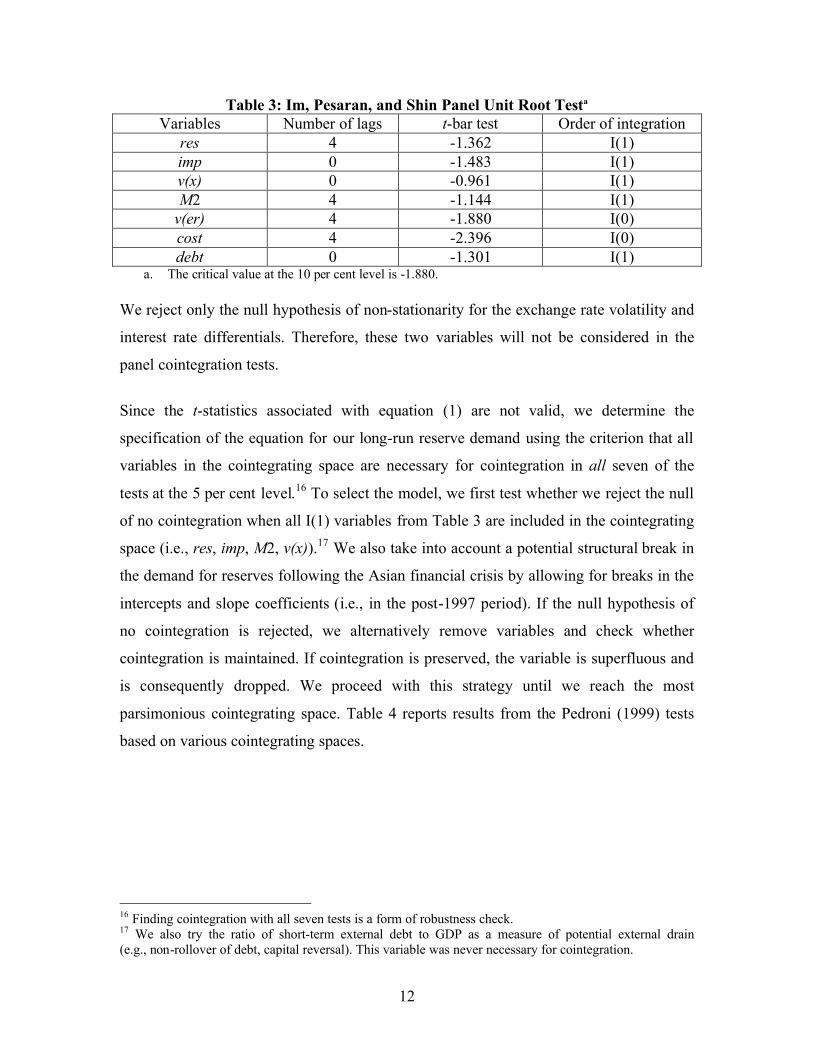
Table 3: Im, Pesaran, and Shin Panel Unit Root Testa

Variables Number of lags t-bar test Order of integration res 4 -1.362 I(1) imp 0 -1.483 I(1) v(x) 0 -0.961 I(1) M2 4 -1.144 I(1)

v(er) 4 -1.880 I(0) cost 4 -2.396 I(0) debt 0 -1.301 I(1)

a. The critical value at the 10 per cent level is -1.880. We reject only the null hypothesis of non-stationarity for the exchange rate volatility and

interest rate differentials. Therefore, these two variables will not be considered in the

panel cointegration tests.

Since the t-statistics associated with equation (1) are not valid, we determine the

specification of the equation for our long-run reserve demand using the criterion that all

variables in the cointegrating space are necessary for cointegration in all seven of the

tests at the 5 per cent level.16 To select the model, we first test whether we reject the null

of no cointegration when all I(1) variables from Table 3 are included in the cointegrating

space (i.e., res, imp, M2, v(x)).17 We also take into account a potential structural break in

the demand for reserves following the Asian financial crisis by allowing for breaks in the

intercepts and slope coefficients (i.e., in the post-1997 period). If the null hypothesis of

no cointegration is rejected, we alternatively remove variables and check whether

cointegration is maintained. If cointegration is preserved, the variable is superfluous and

is consequently dropped. We proceed with this strategy until we reach the most

parsimonious cointegrating space. Table 4 reports results from the Pedroni (1999) tests

based on various cointegrating spaces.

16 Finding cointegration with all seven tests is a form of robustness check. 17 We also try the ratio of short-term external debt to GDP as a measure of potential external drain (e.g., non-rollover of debt, capital reversal). This variable was never necessary for cointegration.

13

Table 4: Panel Cointegration Tests (1980–2003)a Cointegrating space Panel

L-stat Panel D-stat

Panel pp-stat

Panel adf-stat

Group D-stat

Group pp-stat

Group adf-stat

1. res, imp*, M2t-1*, v(x)* -2.346 3.396 2.870 3.001 4.484 3.856 4.108

2. res, imp*, M2 t-1*, v(x) -1.935 2.614 2.016 2.164 3.730 3.013 3.277

3. res, imp*, M2 t-1* -1.809 1.854 1.019 1.170 2.705 1.552 1.885

4. res, imp*, M2 t-1, v(x) -1.302 1.730 0.891 1.044 2.810 1.729 1.999

5. res, imp, M2 t-1*, v(x) -1.642 2.149 1.662 1.760 3.247 2.686 2.927

a. All reported values are distributed N(0,1) under the null hypothesis of no cointegration. Critical values at the 10, 5, and 1 per cent level are 1.645, 1.96, and 2.575, respectively. res is total reserves minus gold deflated by nominal GDP (in logs), imp is the ratio of imports to GDP (in logs), M2t-1 is the lagged ratio of broad money to GDP (in logs), and v(x) is the volatility of export receipts. “*” means that a structural break in the slope coefficient is allowed. The underlying regression model also includes country fixed effects.

With specifications 1 and 2, we reject the null hypothesis of no cointegration at the 5 per

cent level. The break in the coefficient of v(x) is therefore superfluous and this variable

can be excluded from the cointegrating space. From specifications 3, 4, and 5, we note

that the other variables and the breaks are not redundant, since removing any of them

reverses the conclusion of the test. Structural breaks in the coefficients of imports to GDP

and money to GDP are therefore necessary to reject the null hypothesis of no

cointegration. This supports the hypothesis of post-crisis break and points to evidence of

a change in central bank behaviour.

Thus, the most parsimonious specifications yielding cointegration include the ratio of

imports to GDP, the ratio of broad money to GDP (lagged, due to potential endogeneity),

the volatility of export receipts, and breaks in the coefficients of imports to GDP as well

as the ratio of broad money to GDP in the post-crisis period (specification 2). The fact

that each of these variables is required to reject the null hypothesis of no cointegration is

evidence that the regressors are statistically significant long-run determinants of reserve

holdings.18 From this, we obtain the following ordinary least squares estimates (d1997 is a

dummy variable that is equal to 1 after 1997 and 0 otherwise):

18 We find that, in addition to being stationary, the residuals from this specification, except for those from India, are all normally distributed according to the Shapiro-Wilk and Shapiro-Francia tests for normality.

14

titititititi xvdMMdimpimpres ,19971,1,1997,,, )(15.0278.0289.033.051.0 ⋅+⋅⋅+⋅+⋅⋅−⋅= −− . (2)

We find a positive coefficient on the ratio of imports to GDP and the ratio of broad

money to GDP. The volatility of export receipts also exhibits a positive coefficient. The

potential for resident-based capital flight from the domestic currency seems to play an

increasingly important role in determining reserve holdings in emerging Asia, since the

coefficient associated with the ratio of broad money to GDP rises by 0.78 in the post-

1997 period. This is consistent with an increasing role for the self-insurance motive

against potential internal drain. Current account developments have, however, less of an

impact on reserve holdings following the Asian crisis, as the coefficient associated with

import propensity declines in the second subperiod. These results are in line with those of

Aizenman, Lee, and Rhee (2004), who find evidence that the rapid integration of Korea

with the global financial system has increased the weight of financial openness and

reduced the weight of trade openness in accounting for the patterns of international

reserves.

We use this demand equation to assess the extent to which international reserves diverge

from their usual economic determinants. The level of reserves predicted by this set of

explanatory variables should not be considered an optimal or desirable level. Rather, it

corresponds to the level of reserves consistent with macroeconomic conditions. Appendix

C provides graphs of the actual and predicted values for each country.

In China (Figure C1), reserves topped US$408 billion in 2003. This is surprisingly lower

than the US$422 billion predicted by the determinants. Elsewhere in Asia, reserves are

slightly above the level suggested by the demand equation: by about US$32 billion in

India, US$2 billion in Korea, US$6 billion in Indonesia, US$11 billion in Malaysia,

US$3 billion in the Philippines, US$6 billion in Thailand, and US$6 billion in Singapore.

On balance, with a positive gap of US$52 billion, reserve holdings in emerging Asia as a

whole are slightly above the level given by their determinants in 2003.

15

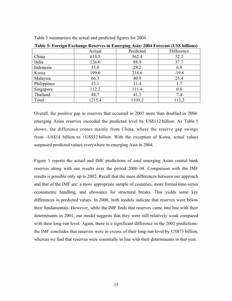
Table 5 summarizes the actual and predicted figures for 2004.

Table 5: Foreign Exchange Reserves in Emerging Asia: 2004 Forecast (US$ billions) Actual Predicted Difference China 614.5 562.4 52.1 India 126.6 88.9 37.7 Indonesia 35.0 28.2 6.8 Korea 199.0 218.6 -19.6 Malaysia 66.3 40.9 25.4 Philippines 13.1 11.4 1.7 Singapore 112.2 111.4 0.8 Thailand 48.7 41.3 7.4 Total 1215.4 1103.2 112.2

Overall, the positive gap in reserves that occurred in 2003 more than doubled in 2004:

emerging Asian reserves exceeded the predicted level by US$112 billion. As Table 5

shows, the difference comes mainly from China, where the reserve gap swings

from -US$14 billion to +US$52 billion. With the exception of Korea, actual values

surpassed predicted values everywhere in emerging Asia in 2004.

Figure 1 reports the actual and IMF predictions of total emerging Asian central bank

reserves along with our results over the period 2000–04. Comparison with the IMF

results is possible only up to 2002. Recall that the main differences between our approach

and that of the IMF are: a more appropriate sample of countries, more formal time-series

econometric handling, and allowance for structural breaks. This yields some key

differences in predicted values. In 2000, both models indicate that reserves were below

their fundamentals. However, while the IMF finds that reserves came into line with their

determinants in 2001, our model suggests that they were still relatively weak compared

with their long-run level. Again, there is a significant difference in the 2002 predictions:

the IMF concludes that reserves were in excess of their long-run level by US$73 billion,

whereas we find that reserves were essentially in line with their determinants in that year.

16

Figure 1: Predicted Reserves in Emerging Asia (2000–04)

Total Reserves(billions of US dollars)

561 578

674

840

1103

486543

678

892

1215

509 540605

400

500

600

700

800

900

1000

1100

1200

1300

2000 2001 2002 2003 2004

BoC Actual IMF

Overall, our model allows for a higher long-run level of reserves in the post-crisis period.

Still, the very strong pace of reserve accumulation over the past two years has put the actual

level of reserves in excess of US$52 and US$112 billion in 2003 and 2004, respectively.

4.3 Results: error-correction model

We further examine the cointegrating vector by estimating a fixed-effects panel error-

correction model for the per cent change in the ratio of reserves to GDP:

∑=

−− +∆+−−+=∆K

kititkktitiiti xyyy

1,1,1, )ˆ( ξψςωφ . (3)

This also allows us to examine the explanatory power of stationary variables that were

dismissed from the cointegration analysis; i.e., exchange rate volatility and opportunity

cost. In addition to these determinants, we consider changes in the variables of the

cointegrating space. Results provide additional evidence of cointegration, with a strongly

significant error-correction term of -0.56 (Table 6). Four lags of the dependent variable

are needed to account for the autoregressive persistence of the series. The residuals are

white noise according to the Ljung-Box Q-statistics. At 56 per cent per year, adjustment

is fairly rapid. These results are broadly consistent with those of Ford and Huang (1994),

who obtain a rate of adjustment of 52 per cent per year for China. Quite surprisingly,

17

aside from lagged values of the dependent variable, none of the aforementioned variables

are statistically significant.

Table 6: Panel Error-Correction Model Coefficient t-stat ecmt-1 -0.56 -5.58 dlres_gdp t-1 0.18 1.89 dlres_gdp t-2 0.08 0.87 dlres_gdp t-3 0.15 1.95 dlres_gdp t-4 -0.10 -1.45 dum crisis 0.36 3.66 R2 40% LB-Q(1) 0.595 LB-Q(4) 0.857

5. Discussion

In this section, we put our results into a broader perspective by examining other costs of

holding reserves that our model cannot take into account. We then discuss the

implications for the U.S. dollar.

Even if reserves had been in line with the identified long-run determinants up to 2004,

there would still be a risk that some key elements are missed by our empirical approach.

Indeed, overaccumulation of reserves entails domestic costs that our model cannot take

into account. These include exchange rate misalignment, loss of monetary control, and

sterilization costs. Taking these costs into account would reduce the desired level of

international reserves, such that the gap relative to actual reserves would be even larger.

Examining the empirical role of such domestic costs is difficult for various reasons. First,

instances of excessive reserves are virtually nonexistent over history. Indeed, until

relatively recently, it was common wisdom that a country with conditional access to

global capital markets would benefit from holding international reserves that were as

large as possible to insure against the risk of capital reversals or sudden stops. Thus, it is

very difficult to empirically establish a causal link between excessive reserve

accumulation and the probability of domestic financial crises based on an historical data

set that reflects an entirely different paradigm. Second, from an econometric perspective,

18

these costs are endogenous. They are the consequence, not the cause, of excessive

reserves. As such, any proxy for these costs cannot be used to explain reserves unless

they have some kind of forward-looking or expected component. To address these issues,

we would need to perform policy or welfare analyses under a general-equilibrium

framework.

5.1 Exchange rate misalignment

Excessive reserves may be harmful when the rapid accumulation is a consequence of

adopting and maintaining a fixed exchange rate, as seems to be the case for some Asian

countries (Osakwe and Schembri 1998). Fixed exchange rates and higher reserves may

indeed increase the vulnerability to a crisis, since economic agents may perceive them as

an implicit guarantee and may not take sufficient insurance against exchange rate

variability. Moreover, an undervalued exchange rate can have harmful effects on growth

and welfare, by reducing consumption, inducing overinvestment in the traded goods

sector, lowering domestic investment, and excessively increasing exposure to external

shocks.19

5.2 Loss of monetary control

The rapid accumulation of reserves can generate inflation. The authorities’ ability to

sterilize capital inflows is limited. For instance, in China in 2004, only about half of the

liquidity arising from the increase in international reserves was sterilized. Rapid credit

expansion and higher inflation could also lead to speculative bubbles, which might

jeopardize domestic financial stability. The longer the authorities attempt to resist market

pressures, the more difficult it becomes for them to retain monetary control. At some

point, Asian central banks will have to either abandon their efforts to peg their currencies

or lose control of monetary and financial expansion. Prasad, Rumbaugh, and Wang

(2005) highlight these different costs and argue that it is typically better to allow the

required adjustment to take place through changes in the nominal exchange rate than

19 Global savings could be misallocated, with overinvestment in export industries in Asia and under-investment in the traded goods sector in the United States.

19

through inflation. Inflationary dynamics can pose serious risks because expectations of

rising inflation can become entrenched, particularly in developing economies.

5.3 Sterilization costs

Sterilization is costly, being roughly equal to the interest paid on the country’s public

debt minus the interest earned on reserves (typically, the interest rate on the

U.S. Treasury debt). To the extent that domestic interest rates are above the rate of return

on the reserve asset, the holding of reserves entails quasi-fiscal costs. According to the

IMF, the cost of sterilizing a reserve accumulation of 10 per cent of GDP can range from

zero to 1 per cent of GDP, depending on the interest spread and the expected exchange

rate depreciation. In order to continuously sterilize inflows, the monetary authority has to

offer ever-increasing interest rates, which would dampen domestic demand.

Consequently, economic growth would likely be reduced following an episode of

massive and prolonged sterilization.

5.4 Implications for the U.S. dollar

Overall, our empirical results for 2003 and 2004, combined with the aforementioned cost

considerations, indicate that, ceteris paribus, a slowdown in the speed of accumulation of

reserves is likely. This implies negative risks for the U.S. dollar. Although the error-

correction model suggests that adjustment can be relatively quick, changes in holding

policies might actually be very gradual in the current context. Indeed, the amount of

reserve assets held by Asian central banks is so large that any change in holding policies

could have a substantial impact on the U.S. dollar and consequently on the balance sheets

of Asian central banks. To avoid large capital losses, Asian central banks will be very

cautious when slowing the rate of reserve accumulation. The recent decision by the Bank

of China to adopt a new basket to which to peg its currency reflects this cautious

approach. As a result, the chances of Asian central banks triggering a rapid depreciation

of the U.S. dollar are not very high.

The currency composition of reserve stocks may pose an additional risk for the U.S.

dollar. It is possible that, from the standpoint of international diversification, the

20

portfolios of Asian central banks would reveal an overweight in dollar assets.20 Ceteris

paribus, diversifying away from the dollar would reduce capital losses in the event of a

reduction in reserve holdings (autonomous or coming from a currency revaluation). There

are signs that central banks are currently losing their appetite for U.S. debt, as they appear

to be reducing their dollar holdings in favour of the euro. For instance, a recent survey of

59 central banks by Pringle and Carver (2005) shows that, in 2004, 70 per cent of

respondents increased their euro holdings, while 52 per cent reduced their dollar

holdings. This is, however, only anecdotal evidence. Data on the currency breakdown of

central banks’ balance sheets is confidential, precluding any formal analysis of the

currency composition of reserves.

Using unpublished IMF-World Bank data, a study by Dooley, Lizondo, and Mathieson

(1989), updated by Eichengreen and Mathieson (2000), examines the determinants of the

currency composition of reserves for developing countries. They find that the

composition of reserves is responsive to the choice of currency peg, the identity of the

dominant trading partner, and the composition of foreign debt. More importantly, they

find that the currency composition of reserves is remarkably stable over time. This is not

surprising, given that variables such as trading relationships and the composition of

foreign debt give evidence of substantial inertia. Thus, the currency composition of

reserves appears to evolve only gradually, so that a radical currency reallocation of

reserves is not very likely to happen within a short period of time. Therefore, although

the outlook for the U.S. dollar may not be favourable from the standpoint of the currency

composition of reserves, risks of an abrupt dollar depreciation coming from this factor

remain limited.

6. Conclusion

We have examined the issue of reserve accumulation by central banks in emerging Asia

by estimating a reserve-demand function in a panel of eight Asian emerging-market

economies. Although we accounted for a structural break in the demand for reserves in

20 BIS data reveal that dollar-denominated securities accounted for roughly 70 per cent of total reserves at the end of 2003.

21

the aftermath of the Asian financial crisis, our model could not explain the very strong

pace of reserve accumulation in the past two years. This suggests that, as long as

historical relationships continue to hold, a slowdown in the pace of reserve accumulation

is likely. This finding implies negative risks for the U.S. dollar. However, the substantial

capital losses that Asian central banks would incur if they were to drastically change their

holding policy mitigate the risks of a rapid depreciation of the U.S. dollar triggered by

Asian central banks.

As a future step to this research, it would be useful to have a more rigorous framework in

which to characterize the potential dilemma facing monetary authorities when

accumulating large stockpiles of reserves; i.e., abandon the currency peg or lose control

of monetary and financial expansion. To develop this type of framework, we would need

to construct a theoretical model in which central banks seek to simultaneously minimize

the risks of external as well as internal crises. The empirical counterpart of such a model

could be based on finding an interval for the level of reserve holdings such that the

probability of external and internal crises is simultaneously minimized.

Another area of research could be to examine the interactions between the financial

system and the process of foreign exchange reserve accumulation. Aizenman and Lee

(2005) investigate the micro foundations of the precautionary demand for reserves along

the lines of the Diamond and Dybvig (1983) bank-run model. Also, Velasco (1987)

argues that foreign exchange reserves can be used to support failing banks and other

financial institutions. This suggests that some financial variables, like average non-

performing loans, or the number of bank closures/mergers, could have predictive power

for reserves.

22

References

Aizenman, J. and J. Lee. 2005. “International Reserves: Precautionary Versus Mercantilist Views: Theory and Evidence.” NBER Working Paper No. 11366.

Aizenman, J., Y. Lee, and Y. Rhee. 2004. “International Reserves Management and

Capital Mobility: Policy Considerations and a Case Study of Korea.” NBER Working Paper No. 10534.

Aizenman, J. and N. Marion. 2002. “The High Demand for International Reserves in the

Far East: What’s Going On?” Journal of the Japanese and International Economies 17(3): 370–400.

________. 2004. “International Reserve Holdings with Sovereign Risk and Costly Tax

Collection.” Economic Journal 114(497): 569–91. Bank for International Settlements (BIS). 2000. “Managing Foreign Debt and Liquidity

Risks.” Policy Paper No. 8, BIS Monetary and Economic Department, Basel. Berg, A. and C. Patillo. 1999. “Are Currency Crises Predictable? A Test.” International

Monetary Fund Staff Papers 46(2): 107–28. Bird, G. and R. Rajan. 2003. “Too Much of a Good Thing? The Adequacy of

International Reserves in the Aftermath of Crises.” World Economy 26(6): 873–91. Diamond, D.W. and P.H. Dybvig. 1983. “Bank Runs, Deposit Insurance, and Liquidity.”

Journal of Political Economy 91(3): 401–19. Dooley, M.P., D. Folkerts-Landau, and P. Garber. 2004. “The Revived Bretton Woods

System.” International Journal of Finance and Economics 9(4): 307–13. Dooley, M.P., J.S. Lizondo, and D.J. Mathieson. 1989. “The Currency Composition of

Foreign Exchange Reserves.” IMF Staff Papers 36: 385–434. Edwards, S. 1985. “On the Interest-Rate Elasticity of the Demand for International

Reserves: Some Evidence from Developing Countries.” Journal of International Money and Finance 4(2): 287–95.

Eichengreen, B. and D.J. Mathieson. 2000. “The Currency Composition of Foreign

Exchange Reserves: Retrospect and Prospect.” IMF Working Paper. Fisher, S. 2001. “Opening Remarks.” IMF/World Bank International Reserves: Policy

Issues Forum, Washington DC, 28 April.

23

Ford, J.L. and G. Huang. 1994. “The Demand for International Reserves in China: An ECM Model with Domestic Monetary Disequilibrium.” Economica 61(243): 379–97.

Greenspan, A. 1999. “Currency Reserves and Debt.” Remarks by Chairman Alan

Greenspan before the World Bank Conference on Recent Trends in Reserve Management, Washington, 29 April.

Gutierrez, L. 2003. “On the Power of Panel Cointegration Tests: A Monte Carlo

Comparison.” Economics Letters 80(1): 105–11. Heller, H.R. 1966. “Optimal International Reserves.” Economic Journal 76(302):

296–311. Heller, R.H. and M.S. Khan. 1978. “The Demand for International Reserves Under Fixed

and Floating Exchange Rates.” International Monetary Fund Staff Papers 25(4): 623–49.

Higgins, M. and T. Klitgaard. 2004. “Reserve Accumulation: Implications for Global

Capital Flows and Financial Markets.” Federal Reserve Bank of New York Current Issues in Economics and Finance 10(10): 1–8.

Im, K.S., M.H. Pesaran, and Y. Shin. 2003. “Testing for Unit Roots in Heterogeneous

Panels.” Journal of Econometrics 115(1): 53–74. International Monetary Fund (IMF). 2003. “Are Foreign Exchange Reserves in Asia Too

High?” World Economic Outlook (September): 64–77. Kao, C. 1999. “Spurious Regression and Residual-Based Tests for Cointegration in Panel

Data.” Journal of Econometrics 90(1): 1–44. Krugman, P. 1979. “A Model of Balance-of-Payments Crises.” Journal of Money, Credit,

and Banking 11(3): 311–25. Landell-Mills, J.M. 1989. “The Demand for International Reserves and their Opportunity

Cost.” International Monetary Fund Staff Papers 36(3): 107–32. Lane, P.R. and D. Burke. 2001. “The Empirics of Foreign Reserves.” Open Economy

Review 12(4): 423–34. Lee, J. 2005. “Insurance Value of International Reserves, an Option Pricing Approach.”

International Monetary Fund, Washington. Lizondo, J. and D. Mathieson. 1987. “The Stability of the Demand for International

Reserves.” Journal of International Money and Finance 6(3): 251–82.

24

Mendoza, R.U. 2004. “International Reserve-Holding in the Developing World: Self Insurance in a Crisis-Prone Era?” Emerging Markets Review 5(1): 61–82.

Newey, W.K. and K.D. West. 1987. “A Simple Positive-Definite Heteroskedasticity and

Autocorrelation Consistent Covariance Matrix.” Econometrica 55(3): 703–8. Osakwe, P. and L. Schembri. 1998. “Currency Crises and Fixed Exchange Rates in the

1990s: A Review.” Bank of Canada Review (Autumn): 23–38. Pedroni, P. 1999. “Critical Values for Cointegration Tests in Heterogeneous Panels With

Multiple Regressors.” Oxford Bulletin of Economics and Statistics, special issue: 653–70.

________. 2004. “Panel Cointegration: Asymptotic and Finite Sample Properties of

Pooled Time Series Tests with an Application to the PPP Hypothesis.” Economic Theory 20(3): 597–625.

Prasad, E., T. Rumbaugh, and Q. Wang. 2005. “Putting the Cart Before the Horse?

Capital Account Liberalization and Exchange Rate Flexibility in China.” International Monetary Fund Policy Discussion Paper.

Pringle, R. and N. Carver. 2005. “Trends in Reserve Management – Results of a Survey

of Central Banks.” In RBS Reserve Management Trends 2005. London: Central Banking Publications Ltd.

Velasco, A. 1987. “Financial Crises and Balance of Payments Crises: A Simple Model of

the Southern Cone Experience.” Journal of Development Economics 27(1-2): 263–83.

Warnock, F. and V.C. Warnock. 2005. “International Capital Flows and U.S. Interest

Rates.” International Finance Discussion Paper No. 840, Board of Governors of the Federal Reserve System.

25

Appendix A: Stylized Facts

Figure A1: Global Reserve Stocks (billions of U.S. dollars)

0

500

1000

1500

2000

2500

Develo

ped c

ountr

ies Japa

n

Euro ar

ea

Develo

ping c

ountr

ies Africa

Asia

Europ

e

Middle

East

Wes

tern H

emisp

here

19992003

Figure A2: International Reserves as a Percentage of GDP

0%5%

10%15%20%25%30%35%40%45%50%

1981

1983

1985

1987

1989

1991

1993

1995

1997

1999

2001

2003

0%5%10%15%20%25%30%35%40%45%50%

China

India

Indonesia

Korea

Malaysia

Philippines

Thailand

26

Figure A3: Regional Distribution of Reserves

Figure A4: Ratio of Reserves to Short-Term External Debt

0

2

4

6

8

10

12

1990

1991

1992

1993

1994

1995

1996

1997

1998

1999

2000

2001

2002

2003

China

India

Indonesia

South Korea

Malaysia

Philippines

Thailand

Singapore

1980

8%

20%

16%

9%13%

9%

5%

20%

2003

45%

11%4%

17%

5%

2%

5%11%

China

India

Indonesia

Korea

Malaysia

Philippines

Thailand

Singapore

27

28

Appendix B: Panel Cointegration Statistics (Pedroni 1999)

1. Panel v-stat:

1

21,

1 1

211

2/32 ˆˆ−

−= =

−

∑ ∑ ti

N

i

T

ti eLNT

2. Panel r-stat: ( )∑ ∑∑ ∑= =

−−

−

−= =

− −∆

N

i

T

tititiiti

N

i

T

ti eeLeLNT

1 1,1,

211

1

21,

1 1

211

ˆˆˆˆˆˆ λ

3. Panel pp-stat: ( )∑ ∑∑ ∑= =

−−

−

−= =

− −∆

N

i

T

tititiiti

N

i

T

tiTN eeLeL

1 1,1,

211

2/1

21,

1 1

211

2,

ˆˆˆˆˆˆ~ λσ

4. Panel adf-stat: ∑ ∑∑ ∑= =

−−

−

−= =

−∗ ∆

N

i

T

ttitiiti

N

i

T

tiTN eeLeLs

1 1

*,

*1,

211

2/1

2*1,

1 1

211

2, ˆˆˆˆˆ~

5. Group r-stat: ( )∑∑ ∑=

−

−

= =−

− −∆

T

tititi

N

i

T

iti eeeTN

1,1,

1

1 1

21,

2/1 ˆˆˆˆ λ

6. Group pp-stat: ( )∑∑ ∑=

−

−

= =−

− −∆

T

tititi

N

i

T

ttii eeeN

1,1,

2/1

1 1

21,

22/1 ˆˆˆˆˆ λσ

7. Group adf-stat: ∑∑ ∑=

−

−

= =−

− ∆

T

ttiti

N

i

T

ttii eeesN

1

*,

*1,

2/1

1 1

2*1,

2*2/1 ˆˆˆˆ

29

where,

∑∑+=

−=

+

−=T

ststiti

k

s ii

i

ks

T 1,,

1

ˆˆ1

11ˆ µµλ ,

∑=

≡T

ti tiT

s1

22,

ˆ1ˆ µ ,

iii s λσ ˆ2ˆˆ 22 += ,

∑=

−≡N

iiiTN L

N 1

2211

2, ˆˆ1~ σσ ,

∑=

≡T

ttii T

s1

2*,

2* 1ˆ µ ,

∑=

≡N

iiTN s

Ns

1

2*2*, ˆ1~

,

∑∑ ∑+=

−= =

+

−+=T

ststiti

T

t

k

s itii

i

ks

TTL

1,,

1 1

2,

211 ˆˆ

11

2ˆ1ˆ ηηη ,

and where the residuals µ and η are obtained from the following regressions:

titiiti ee ,1,, ˆˆˆˆ µγ += − ,

*,

1,,1,, ˆˆˆˆˆˆ ti

K

kktikitiiti

i

eee µγγ ∑=

−− +∆+= ,

∑=

+∆=∆M

mtitmimti xby

1,,, ˆˆ η .

30

Appendix C: Predicted Reserves

Figure C1: China

China Reserves(billions of U.S. dollars)

0

100

200

300

400

500

600

700

1981

1983

1985

1987

1989

1991

1993

1995

1997

1999

2001

2003

Actual Predicted

Figure C2: India

India Reserves(billions of U.S. dollars)

0

20

40

60

80

100

120

140

1981

1983

1985

1987

1989

1991

1993

1995

1997

1999

2001

2003

Actual Predicted

31

Figure C3: Indonesia

Indonesia Reserves(billions of U.S. dollars)

0

5

10

15

20

25

30

35

4019

81

1983

1985

1987

1989

1991

1993

1995

1997

1999

2001

2003

Actual Predicted

Figure C4: Korea

Korea Reserves(billions of U.S. dollars)

0

50

100

150

200

250

1981

1983

1985

1987

1989

1991

1993

1995

1997

1999

2001

2003

Actual Predicted

32

Figure C5: Malaysia

Malaysia Reserves(billions of U.S. dollars)

0

10

20

30

40

50

60

70

1981

1983

1985

1987

1989

1991

1993

1995

1997

1999

2001

2003

Actual Predicted

Figure C6: Philippines

Philippines Reserves(billions of U.S. dollars)

0

2

4

6

8

10

12

14

16

1981

1983

1985

1987

1989

1991

1993

1995

1997

1999

2001

2003

Actual Predicted

33

Figure C7: Thailand

Thailand Reserves(billions of U.S. dollars)

0

10

20

30

40

50

60

1981

1983

1985

1987

1989

1991

1993

1995

1997

1999

2001

2003

Actual Predicted

Figure C8: Singapore

Singapore Reserves(billions of U.S. dollars)

0

20

40

60

80

100

120

1981

1983

1985

1987

1989

1991

1993

1995

1997

1999

2001

2003

Actual Predicted

34

Figure C9: Total

Emerging Asia Reserves(billions of U.S. dollars)

0

200

400

600

800

1000

1200

140019

81

1983

1985

1987

1989

1991

1993

1995

1997

1999

2001

2003

Actual Predicted

Bank of Canada Working PapersDocuments de travail de la Banque du Canada

Working papers are generally published in the language of the author, with an abstract in both officiallanguages. Les documents de travail sont publiés généralement dans la langue utilisée par les auteurs; ils sontcependant précédés d’un résumé bilingue.

Copies and a complete list of working papers are available from:Pour obtenir des exemplaires et une liste complète des documents de travail, prière de s’adresser à :

Publications Distribution, Bank of Canada Diffusion des publications, Banque du Canada234 Wellington Street, Ottawa, Ontario K1A 0G9 234, rue Wellington, Ottawa (Ontario) K1A 0G9E-mail: publications@bankofcanada.ca Adresse électronique : publications@banqueducanada.caWeb site: http://www.bankofcanada.ca Site Web : http://www.banqueducanada.ca

20052005-37 Quantity, Quality, and Relevance:

Central Bank Research, 1990–2003 P. St-Amant, G. Tkacz, A. Guérard-Langlois, and L. Morel

2006-36 The Canadian Macroeconomy and the Yield Curve:An Equilibrium-Based Approach R. Garcia and R. Luger

2005-35 Testing the Parametric Specification of the DiffusionFunction in a Diffusion Process F. Li

2005-34 The Exchange Rate and Canadian Inflation Targeting C. Ragan

2005-33 Does Financial Structure Matter for theInformation Content of Financial Indicators? R. Djoudad, J. Selody, and C. Wilkins

2005-32 Degree of Internationalization and Performance:An Analysis of Canadian Banks W. Hejazi and E. Santor

2005-31 Forecasting Canadian GDP: Region-Specificversus Countrywide Information F. Demers and D. Dupuis

2005-30 Intertemporal Substitution in Macroeconomics: Evidence froma Two-Dimensional Labour Supply Model with Money A. Dib and L. Phaneuf

2005-29 Has Exchange Rate Pass-Through Really Declined in Canada? H. Bouakez and N. Rebei

2005-28 Inflation and Relative Price Dispersion in Canada:An Empirical Assessment A. Binette and S. Martel

2005-27 Inflation Dynamics and the New Keynesian Phillips Curve:An Identification-Robust Econometric Analysis J.-M. Dufour, L. Khalaf, and M. Kichian

2005-26 Uninsured Idiosyncratic Production Risk with Borrowing Constraints F. Covas

2005-25 The Impact of Unanticipated Defaults in Canada’s Large Value Transfer System D. McVanel

2005-24 A Search Model of Venture Capital, Entrepreneurship,and Unemployment R. Boadway, O. Secrieru, and M. Vigneault

2005-23 Pocket Banks and Out-of-Pocket Losses: Links between Corruptionand Contagion R.H. Solomon