Banco Hidraulico
84
University of Puerto Rico, Mayagüez Campus Department of Chemical Engineering Mayagüez, Puerto Rico Hydraulic Bench: Jet Impact, Flow through Orifices and Flow through Weirs INQU 4034-020 Fabiola Semidei Ortiz (leader) Carla Serrano Vélez (leader) Emmanuel Chamorro (assistant) Humberto González (assistant)
-
Upload
emmanuel-jesus-chamorro -
Category
Documents
-
view
277 -
download
1
Transcript of Banco Hidraulico
University of Puerto Rico, Mayagüez Campus
Department of Chemical Engineering
Mayagüez, Puerto Rico
Hydraulic Bench: Jet Impact, Flow through Orifices and Flow through Weirs
INQU 4034-020
Fabiola Semidei Ortiz (leader)
Carla Serrano Vélez (leader)
Emmanuel Chamorro (assistant)
Humberto González (assistant)
Date experimental work started: 3/17/2014
Date experimental work ended: 3/24/2014
Date written report is submitted: 4/2/2014

Table of ContentsTable of Contents........................................................................................................................................2
List of Tables...............................................................................................................................................4
List of Figures.............................................................................................................................................5
Summary.....................................................................................................................................................8
Goals and Objectives...................................................................................................................................9
Goals 9
Objectives 9
Nomenclature............................................................................................................................................10
Theory.......................................................................................................................................................12
Fluids 12
Macroscopic Mass & Momentum Balance 13
Jet Impact 15
Bernoulli’s Equation 16
Torricelli’s Law 18
“Vena Contracta” Effect 19
Flow Through Orifice: Steady State 20
Flow Through Orifice: Unsteady State 22
Safety Aspects...........................................................................................................................................24
General Aspects 24
Specific Aspects 24
Equipment Description..............................................................................................................................26
Hydraulic Bench 26
Jet Impact Equipment27
Orifice and Weirs Equipment 28
Experimental Procedure............................................................................................................................30
2

Hydraulic Bench 30
Jet Impact 30
Flow through orifice 31
Steady State.......................................................................................................................................32
Unsteady State...................................................................................................................................32
Rectangular weir 32
Data Sheet.................................................................................................................................................34
Sample Calculations..................................................................................................................................40
Jet Impact (Plane target) 40
Flow through orifice (Steady State) 42
Flow through orifice (Unsteady State) 45
Flow through a rectangular Weir 47
Results.......................................................................................................................................................49
Jet Impact 49
Plane Target.........................................................................................................................................49
Hemispherical Target...........................................................................................................................50
Flow through Orifices 52
Flow through Rectangular Weirs 56
Discussion of Results................................................................................................................................61
Conclusions and Recommendations..........................................................................................................63
References.................................................................................................................................................64
Appendix...................................................................................................................................................64
3

List of TablesTable 1: Data Used for Sample Calculations.................................................................................40
Table 2: Flow Difference for all Weights......................................................................................41
Table 3: Experimental Data for a height of 0.353m......................................................................42
Table 4: Volumetric flow rate data for Steady State.....................................................................44
Table 5: Data for determination of CD..........................................................................................45
Table 6: Data for the determination of CD....................................................................................47
Table 7: Comparison between theoretical slope and experimental slope......................................49
Table 8: Comparison between slopes............................................................................................50
Table 9: Comparison between slopes............................................................................................51
Table 10: Comparison between slopes..........................................................................................51
Table 11: Squared horizontal distance vs. vertical distance..........................................................52
Table 12: Discharge and velocity coefficients per height selected................................................53
Table 13: Squared volumetric flow vs height................................................................................53
Table 14: Slope, CD, AO, CD, theo, diameter and error percentage............................................53
Table 15: Difference of squared heights, radius area, CD, exp, CD, theo, slope, error percentage................................................................................................................................................55
Table 16: Calculated volumetric flows, height and height raised to the (3/2)th power.................56
Table 17: Error percentage for CD................................................................................................57
Table 18: Volumetric flows and heights........................................................................................57
Table 19: Volumetric flows and heights........................................................................................58
Table 20: Error percentage for CD................................................................................................59
Table 21: Volumetric flows and heights........................................................................................59
Table 22: Error percentage for CD................................................................................................60
4

List of FiguresFigure 1: Toothpaste....................................................................................................................................11
Figure 2: Quicksand.....................................................................................................................................12
Figure 3:Plot of Shearing Stress (τ) versus Rate of Shearing Strain (du/dy)...............................................12
Figure 4: Macroscopic model of a fluid.......................................................................................................13
Figure 5: Macroscopic balance in a changing area, with force balance......................................................14
Figure 6: Plane taget body diagram.............................................................................................................14
Figure 7: Fluid through changing area model..............................................................................................16
Figure 8: Flow through Orifice....................................................................................................................18
Figure 9: Fluid through a tube with an orifice.............................................................................................19
Figure 10: Fluid exiting tank through an orifice covering distance x and y................................................20
Figure 11: Rectangular Weir with length L and water height H..................................................................22
Figure 12 Safety Goggles.............................................................................................................................23
Figure 13: Lab Coat.....................................................................................................................................23
Figure 14: Stairs...........................................................................................................................................24
Figure 15: Electric Hazard...........................................................................................................................24
Figure 16: Vernier Needle...........................................................................................................................25
Figure 17: Acetone.......................................................................................................................................25
Figure 18: Hydraulic Bench Apparatus.......................................................................................................26
Figure 19: Jet Impact Diagram....................................................................................................................27
Figure 20: Jet Impact Apparatus..................................................................................................................27
Figure 21: Jet Impact Targets......................................................................................................................27
Figure 22: Jet Impact Standardized Weights..............................................................................................27
Figure 23: Orifice and Weir Apparatus Diagram........................................................................................28
Figure 24: Weir Apparatus...........................................................................................................................28
Figure 25: Orifices.......................................................................................................................................29
Figure 26: Weir Instruments........................................................................................................................29
Figure 27: Hydraulic Bench.........................................................................................................................30
Figure 28: Jet Impact Apparatus..................................................................................................................31
Figure 29: Flow through Orifice Front View...............................................................................................31
5

Figure 30: Flow over Weir...........................................................................................................................33
Figure 31: Flow through an Orifice for h=0.381 (m)..................................................................................43
Figure 32: Q2 (m6/s2) vs h (m) plot data for tank water height..................................................................44
Figure 33: Flow through an orifice (Unsteady State)..................................................................................46
Figure 34: Plot of Q vs H3/2 for different positions......................................................................................47
Figure 35: Mass vs. the difference of the squares of the volumetric flows.................................................49
Figure 36: Mass vs. the difference of the squares of the volumetric flows................................................50
Figure 37: Mass vs. the difference of the squares of the volumetric flows: plane target...........................51
Figure 38: Mass vs. the difference of the squares of the volumetric flows.................................................51
Figure 39: The three different flows selected for the orifice experiment vs. height....................................52
Figure 40: Squared horizontal distance vs. vertical distance.......................................................................54
Figure 41: Squared horizontal distance vs. vertical distance.......................................................................54
Figure 42: Squared horizontal distance vs. vertical distance.......................................................................55
Figure 43: Time vs. difference of squared heights......................................................................................56
Figure 44: Volumetric flow vs. H3/2...........................................................................................................57
Figure 45: Q (m3/s) vs H3/2 (m3/2)............................................................................................................58
Figure 46: Volumetric flow vs. H3/2...........................................................................................................59
Figure 47: Volumetric flow vs. H3/2...........................................................................................................60
6

SummaryThree experiments were conducted with the purpose of observing the abidance by the
laws of conservation of mass, energy and momentum of fluids: jet impact on targets of different
geometries, flow through an orifice, and flow over a rectangular weir.
For the jet impact experiment, a water target with two different geometries (plane and
hemispherical), were compared. A much greater force was needed to counteract the force
produced by a jet impacting a hemispherical target rather than a plane target. Linear relations
between mass added (mp) and flow rates (Q2 – Qi2) gave R2 values ranging from 0.979 to 0.982.
The error percentages obtained were in the range 18.1% and 31.51% for the plane target for the
first and second trials, respectively, and in the range of 12.3% and 18.13% for the first and
second trials, respectively, for the hemispherical target.
The discharge coefficient (CD) and velocity coefficient (CV) were obtained for flow
through an orifice. The CD values were obtained under steady and unsteady state conditions.
Different length measurements were taken in order to obtain the CV values. The error percentages
for the CD values were 17.78% for steady state and 18.91% for unsteady state. The error
percentages for CV values range from 5.73% to 19.82%.
In the last part of the experiment, the relation between the volumetric flow rate and the
H3/2 was studied for rectangular weir. The error percentages for the discharge coefficient (CD)
were obtained to be 16.67% at the opening height and 2.13% at the middle height for the first
run, and 3.41% at the opening height and 13.39% at the middle height for the second run. After
the experimental procedure was completed it was concluded that the fluid behavior was affected
7

by the geometries. Also, that the discharge and velocity coefficient can be determined using the
Bernoulli equation.
Goals and Objectives
Goals
The goal of this experiment was to study the different principles of fluid theory such as mass,
momentum and mechanical energy balances and implement them in different geometries.
Objectives
The goal previously mentioned, was reached by accomplishing different experiments and
applying its respective laws trough the Jet impact, Flux by Orifice and Flux by Weir
experiments. The theory equations that describe the force executed by a water jet impact over
targets of different geometries. Also the discharge coefficient (CD) and the speed coefficient (CV)
of a orifice were determined. A relationship between the height of the water and the flow of
water entering a weir was determine as well and compared with literature results.
8

NomenclatureSymbol Definition Units
A flow area m2
a acceleration m/s2
A0 Orifice Area m2
AR Cross Sectional Area m2
Avc Area “Vena Contracta” m2
Contraction Factor -
Discharge Coefficient -
Velocity Factor -
9

F force kg/m s2
force of the solid surface on the fluid kg/m s2
gravity force vector m/s2
H height m
h vertical distance m
m mass kg
mass flow rate kg/s
rate of increase of momentum Kg m/s
total mass of the fluid kg
P pressure kg/m s2
Q Volumetric Flow Rate m3/s
surface of the plane m2
t time s
u velocity m/s
vector symbol -
V fluid Velocity m/s
velocity of the fluid m/s
Vi Ideal Velocity m/s
Vvc Velocity Vena Contracta m2/s
x horizontal distance m
y vertical distance m
10

z fluids height above a reference point M
γ shear strain rate
shear viscosity Pa*s or kp·s/cm2
ρ fluid density Kg/m3
shear stress Pa
Theory
FluidsA fluid is a substance that deforms continuously when acted on by a shearing stress of
any magnitude. Shearing stress is a force applied tangential to a surface. It is important to note
that when applying a shear stress to some solids, for example some metals, they will have an
initial deformation but not continuous. This is why it is categorized as a solid and not a fluid.
There are other substances that are categorized as fluids but act somewhat as solids. A good
example is a household product, toothpaste.
Figure 1: Toothpaste
With a small shear stress applied, it acts as a solid; but after a certain amount of shear stress is
applied, it will act as a fluid. Another example could be quicksand (mixture of sand and water)
where the harder a shear stress is applied, the more viscous it becomes.
11

Figure 2: Quicksand
Fluids with similar characteristics as these are called Non-Newtonian fluids. If shearing stress
versus rate of shearing strain is plotted, it can be seen that the viscosity of these fluids is not
linearly proportional to shear stress. For Newtonian fluids it can be seen, in this same plot, that
the viscosity is linearly proportional to shear stress.
Figure 3:Plot of Shearing Stress (τ) versus Rate of Shearing Strain (du/dy)
These fluids are named after Sir Isaac Newton (1642-1727) who explored various aspects of
fluid resistance, for example viscosity. Based upon his observations, he defined the relationship
between shear stress and shear rate of a fluid subjected to mechanical stress.
Eq.1
12

Where τ is the shear stress, µ is the viscosity, and du/dy is the derivative of the velocity parallel
to the direction of the shear stress.
As seen in Newton’s Law of Viscosity, the viscosity is independent of the shear rate; therefore
this law does not apply to Non-Newtonian fluids.
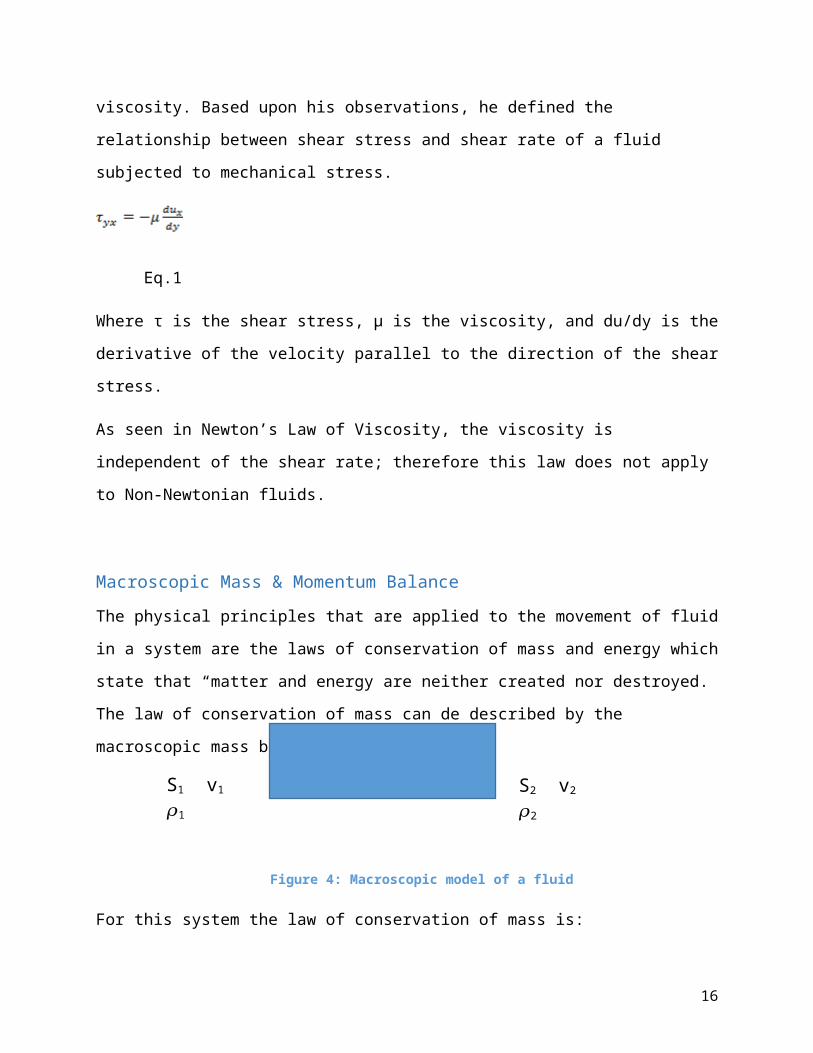
Macroscopic Mass & Momentum BalanceThe physical principles that are applied to the movement of fluid in a system are the laws of
conservation of mass and energy which state that “matter and energy are neither created nor
destroyed. The law of conservation of mass can de described by the macroscopic mass balance in
a system.
For this system the law of conservation of mass is:
Eq. 2
Where is the rate of increase of mass, is the rate of mass entering, and is
the rate of mass exiting.
In a steady state system, where there is no accumulation of mass occurring, the macroscopic
mass balance is:
Eq. 3
The law of conservation of energy is described by a macroscopic momentum balance on a fluid
entering a system.
13
S1 v1 𝜌1 S2 v2 𝜌2
Figure 4: Macroscopic model of a fluid
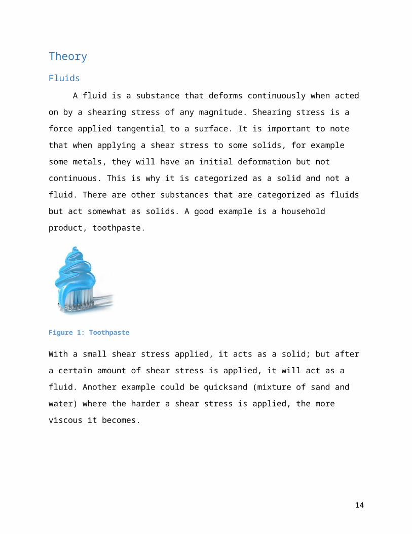
Figure 5: Macroscopic balance in a changing area, with force balance
The law of conservation of momentum is:
Eq. 4
Where is the rate of increase of momentum, is the rate of momentum entering,
is the rate of momentum exiting, is the pressure force on the fluid at
entrance, is the pressure force on fluid at exit, is the force of solid surface on fluid,
and is the force of gravity on fluid.
For this experiment, it is necessary to make some simplifications to this equation. We assume a
steady state system, an open to atmosphere system (no pressure differences), a fluid with
constant density, and the only component of interest being the y axis.
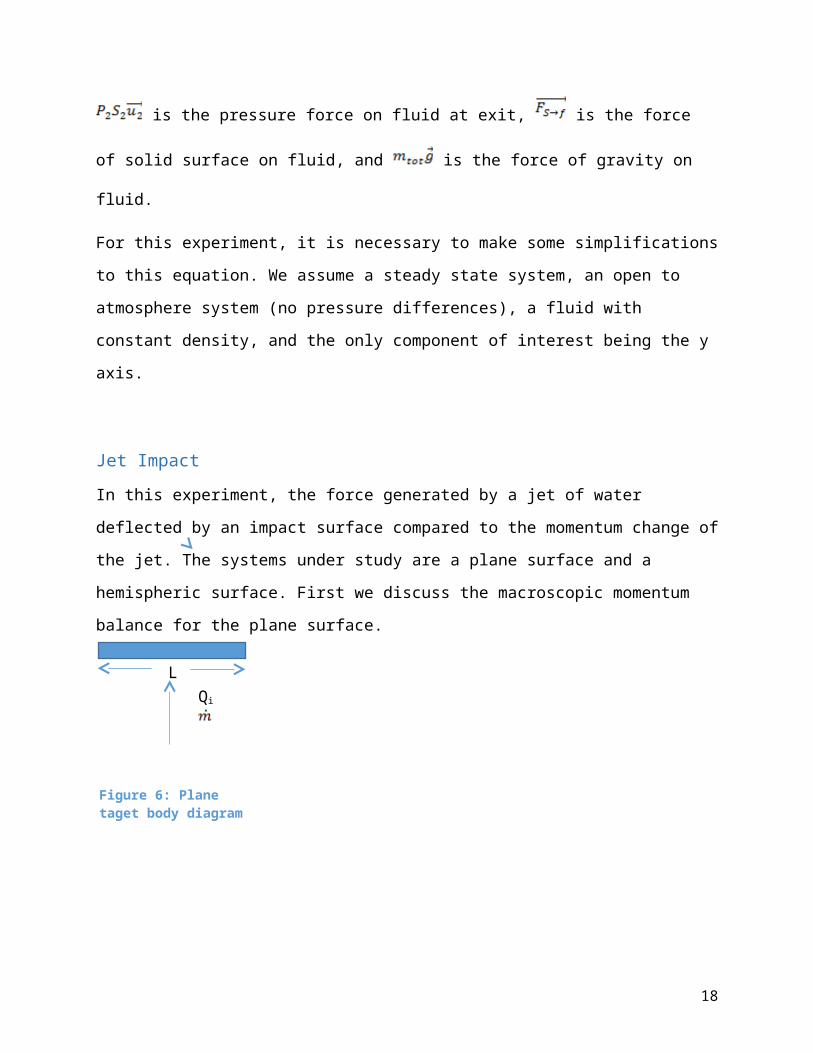
Jet ImpactIn this experiment, the force generated by a jet of water deflected by an impact surface compared
to the momentum change of the jet. The systems under study are a plane surface and a
hemispheric surface. First we discuss the macroscopic momentum balance for the plane surface.
14
LQi
Figure 6: Plane taget body diagram

Fiure. 6 shows a plane surface of length L in which Qi is the volumetric flow, m ̇ is the mass
flow, and V1y is the velocity in the Y direction. .Here we see that when the flow in the Y impacts
the plane surface, the fluid separates into the X direction, therefore, V2y = 0. The macroscopic
momentum balance for this system is:
Eq. 5
Where A is the area of the jet, mtarget is the mass of the target, mweight dish is the mass of the weight
dish, mp is the applied mass, g is the gravity, and mjet is the jet mass. In the calibration experiment
no mass was applied, making mp = 0. Then we can say that:
Eq. 6
When applying a mass to the top of the plane surface, the macroscopic momentum balance can
be simplified to:
Eq. 7
Where Qi was taken from the calibration experiment and Q was the new measured volumetric
flow. Solving for the applied mass:
Eq. 8
15
For the hemispheric surface the same method is used. Here it is important to note that the
average velocity entering <v1> is equal to the average velocity exiting <v2>:
Eq. 9
Making the macroscopic momentum balance:
Eq. 10
Since :
Eq. 11
Adding a weight:
Eq. 12
16

Bernoulli’s Equation
Daniel Bernoulli (1700-1782), a Swiss mathematician and physicist was very influential to the
studies of fluid mechanics. This is all thanks to his principle that states that a rise (fall) in
pressure in a flowing fluid must always be accompanied by a decrease (increase) in the speed,
and conversely, an increase (decrease) in the speed of the fluid results in a decrease (increase) in
the pressure. We study a fluid moving through a system in which a pressure difference occurs as
a result of a change in area.
Figure 7: Fluid through changing area model
Figure 7 shows a fluid with velocity v1 entering though tube of area A1 experiencing pressure P1
and passing with velocity v2 through the contraction of area A2 experiencing pressure P2.
Assuming that the fluid is incompressible and non-viscous and that the flow is smooth (without
turbulence), we can make an energy balance, we come up with Bernoulli’s Equation:
Eq. 13
Where P1 is the pressure experienced at the entrance of the tube, 𝜌is the density of the fluid, v1 is
the velocity of the fluid at the entrance, g is the gravity, z1 is the height at the entrance, P2 is the
pressure experienced at the exit of the tube, v2 is the velocity of the fluid at the exit, and z2 is the
height at the exit.
17
It is important to notice that v2>v1, therefore P2<P1. If both sides of the equation are multiplied by 𝜌, the equation gives us:
Eq. 14
is the pressure energy term, is the kinetic energy per unit volume, is the potential
energy per unit volume term.
Torricelli’s Law
Evangelista Torricelli (1608-1647), an Italian physicist and mathematician, influenced fluid
dynamics by relating the speed of a fluid exiting a cylinder though a small opening with the
height of the fluid above the opening.
Figure 8: Flow through Orifice
Figure 8 shows a fluid flowing through a cylinder and exiting out an orifice at the bottom of the
cylinder. P1 is the pressure at the top of the cylinder, v1 is the velocity of the fluid at the top of the
18

cylinder, z1 is the height of the fluid at the top of the cylinder, 𝜌is the density of the fluid, P2 is
the pressure at the orifice, v2 is the velocity of the fluid at the exit of the orifice, z2 is the height of
the fluid at the orifice. Torricelli’s law states that the velocity of a fluid through an orifice at the
bottom of a cylinder filled to depth h is the same as the speed of that body. This relationship can
be derived with Bernoulli’s equation for an incompressible fluid (𝜌is constant) with frictionless
and steady flow. A notation that will be used is . It is important to remember that the
system is open to atmospheric pressure, therefore . Also the velocity at the top of
the cylinder is negligible, . Deriving the Bernoulli equation from Eq. 13 for this system:
Eq. 15
This gives us:
Eq. 16
Where vi is the ideal velocity.
“Vena Contracta” Effect
“Vena contracta” is the narrowest central flow region of a jet that occurs just downstream to the
orifice of a valve.
19
Figure 9: Fluid through a tube with an orifice
The measurement of the ideal velocity, discussed above, is affected by any type of loss in the
system and by the difference in area between the orifice and the “vena contracta”. In this system
the loss is due to contraction. The factors used to correct the calculations of the ideal velocity are
the velocity factor, Cv, and the contraction factor, Cc.
Eq. 17
Where vactual is the real velocity and videal is the ideal velocity calculated from Eq. 16.
Eq. 18
Where Avc is the area of the “vena contracta” and Ao is the area of the orifice.
The real volumetric flow can also be calculated with these correction factors:
Eq. 19
20

Where vvc is the velocity of the fluid passing though the “vena contracta.”
Defining CD, the discharge factor, as:
Eq. 20
We get that:
Eq. 21
Flow Through Orifice: Steady State
The fluid exiting the recipient through the orifice covers a distance in the X and Y-axes over a
certain amount of time.
Figure 10: Fluid exiting tank through an orifice covering distance x and y
The distance in the Y-axis can be defined as:
21

Eq. 22
Where t is the time for the stream to cover the distance y in the Y-axis.
The distance x in the X-axis covered in that amount of time is:
Eq. 23
Where v is the velocity of the stream.
Solving Eq. 22 for time:
Eq. 24
Combining Eq. 23 and Eq. 24 and solving for velocity:
Eq. 25
Substituting in the Eq. 17:
22

Eq. 26
Leaving x on one side and y on the other side of the equation gives:
Eq. 27
Flow Through Orifice: Unsteady State
In contrast to steady state, during unsteady state no water is being poured into the tank, making
the height dependent on time. In this case, the flow of water exiting the orifice is the same to the
rate of reduction of the volume of water in the tank:
Eq. 28
Where AR is the sectional area of the recipient.
Integrating:
Eq. 29
Flow through a Rectangular Weir
23

A weir is a barrier used to intercept the flow of a liquid in a stream in order to alter its flow. It is
used mostly in rivers to prevent flooding, make them navigable, and to be able to measure the
flow. In our experiment a rectangular notch was studied.
Figure 11: Rectangular Weir with length L and water height H
We changed Eq. 16 for this system by making h=H, where H is the height of the liquid above the
weir, and making vi=v, where v is the velocity of the liquid. The volumetric flow of the liquid is
expressed as:
Eq. 30
Where Q is the volumetric flow of the liquid in the weir and A is the area of the weir.
Substituting in Eq. 26 for v, we get:
Eq. 31
Eq. 32
Integrating Eq. 31:
24

Eq. 33
Eq. 34
It is important to note that the volumetric flow rate of the liquid is linearly proportional to the
height of the liquid above the weir elevated to 3/2, .
Safety Aspects
General Aspects
When people are working in a laboratory there are certain rules that must be followed in
order to create a place safe for all the workers of the laboratory. As a primary rule the worker of
the laboratory must wear appropriate clothing (jeans/long pants,
shirts with sleeves and closed shoes) and also adequate protective
gear like lab coat (Figure 13 ) and safety
goggles (Figure 12 ). If the worker had
long hair, it should be tied. Food, drinks
and smoking are prohibited in the laboratory. Also it’s a responsibility
of all the members of the laboratory to know the location of safety
equipment like the eye wash stations, fire extinguishers, first aid kits,
spill control kits, etc. In case that the laboratory worker will be exposed
to a reactant, he has the responsibility to study and know all the
physical properties of the substance. To do this the worker must refer to the hazard rating chart
or to the MSDS (Material Safety Data Sheet) book. Also it is important to know the locations of
the table of the emergency phone numbers, if it is possible the person can carry this phone
25
Figure 12 Safety Goggles
Figure 13: Lab Coat

number in their personal phone to make the an emergency procedure more effective. While
working in the lab, awareness of the people and equipment in your surroundings is a necessary
precaution.
Specific Aspects
For the hydraulic bench experiment there are other safety aspects that the laboratory
worker must know before beginning the experiment. This
experiment takes place in the second floor of the laboratory;
therefore the worker must be conscious of the stairs (Figure
14 ) and handrails . To avoid any accident use the handrails
to go down or upstairs. Also beware of the second floor
handrails because they are very low, even for a person with
an average height. Since this experiment consists of working
with water, there are some preventing rules that workers must follow to avoid spills and
electrical mishaps. So it is extremely important to be completely dry before work with the
electricity.
26
Figure 15: Electric Hazard
Figure 16: Vernier Needle
Figure 14: Stairs
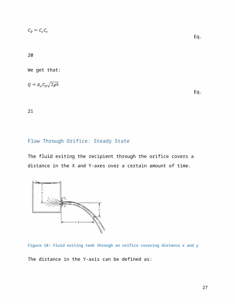
Figure 17: Acetone
Equipment Description
Hydraulic Bench
For each of the experiments performed the hydraulic bench was the source of water flow,
it was necessary to provide a uniform flow of water that could be regulated according to required
conditions. The equipment consists of a measurement tank, a reserve tank, a pump, and the
devices necessary to measure and control the liquid flow as shown in Figure 18. The pump,
which was connected to the reserve tank of 140 L water was suction form the reserve tank and
sent through the tube to the discharge zone. Flexible tubes were used to make the connections of
the hydraulic bench to apparatus used for the specific experiment. The discharge valve controlled
water flow through the tube. The water discharged by the equipment connected to the hydraulic
bench went to the measures tanks. Those tanks were discharged into the reserve tank through
tube. The discharge tube avoids the overflow of the measure tanks. The level of water was
determined introducing a properly marked wood stick via tube. The equipment was turned on
using the electric interrupter.
27
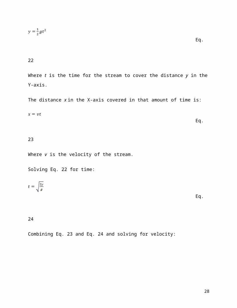
Figure 18: Hydraulic Bench Apparatus
Every time an experiment is performed, it is necessary to check the water level in this tank
to make sure there is enough liquid. It is not sealed hermetically, so work carefully to prevent
water spills. The total volume of water in the tanks can be determined using a calibrated wooden
stick, which is lowered into the tank to make the measurement
Jet Impact Equipment
The jet impact apparatus shown in Figure 19 is an acrylic cylinder with a 1-cm internal diameter
vertical nozzle (2) that is connected to the discharge on top of the hydraulic bench with tube (1).
The water flowing through the nozzle hits a specially shaped target (3) connected to a weight
tray (5) on the lid of the cylinder. An indicator (6) shows the equilibrium position of the weight
tray. When weights are placed on the tray, the water flow must be increased to compensate for
this increase of weight and reach equilibrium again.
28

To maintain constant (atmospheric) pressure within the cylinder, the valve on the lid (8)
must be opened. Water flows out of the apparatus through a drain (7) and fall into the
measurement tank on the hydraulic bench, where the volumetric flow rate can be measured either
with a volumetric flask or with the tanks themselves. While conducting this, weights (Figure 22 )
are used to determine the force needed to counteract the increase in flow rate and experiment
different targets are used throughout the experimentation flat and spherical (Figures 21).
Figure 21: Jet Impact Targets
Figure 22: Jet Impact Standardized Weights
29
Figure 19: Jet Impact Diagram
Figure 20: Jet Impact Apparatus

Orifice and Weirs Equipment
In the apparatus used for flow through orifices and weirs (see Figures 23 and 24), the
water enters the tank through the flexible tube and copper U turn (1). A ring at the top of the
main tank holds the tube in place.
Figure 23: Orifice and Weir Apparatus Diagram
Figure 24: Weir Apparatus
An internal tube inside the main tank prevents it to overflow 11. The main tank has two
exits. The main exit can be closed when necessary (2) (e.g. when working with orifice). The
30
Weir

other exit is for the installation of the orifices (3). A crystal tube located on one side of the tank
can measure the height of the water level inside the main tank (4). Water flows from the main
tank to the discharge tank, and then flows back to the measurement tank through a drain (5). If
the main exit is left open water will flow directly from the main tank to the discharge tank
through grids (6) and over the weir (7). Finally, it will flow into the measure tank. The Vernier
scale (9) is placed on top of the rails (8) and is used to measure the vertical distance of the water
over the weir.
Experimental Procedure
Hydraulic Bench
For every experiment the process began by making sure the water tank was at the correct
water level utilizing the calibrated wooden stick. Afterwards the adequate connections to the
apparatus that was be used for specific experiment was made utilizing the flexible tubes, and
making sure that the water discharged into the tank.
31
Figure 26: Weir Instruments Figure 25: Orifices

Figure 27: Hydraulic Bench
Jet Impact
For this experiment two trials were done, with an hemispherical and plane target. The jet
impact apparatus was carefully located on place. The lid of the cylinder was removed in order to
install the plane target, the first to be used. Afterwards the lid was closed and the cylinder was
calibrated using a bubble meter. The pump was started before the apparatus was leveled. The
control valve was opened slowing as the water entered the apparatus. The water flow was
regulated until the weight tray was close to the indicator in the lid as for the initial equilibrium
obtained.
The initial volumetric flow rate, Qi, was measured with any mass over the target. This
was attained by taking the average time for a certain quantity of volume to be collected in the
tank. The initial flow rate was acquired with no weight added to the tray and it became the
reference measurement for the flow.
The maximum allowed weight was located on the weight tray. The water flow was
adjusted again to reach the equilibrium position showed by the indicator. Once steady state is
reached, the new volumetric flow is measured. The same procedure was done but each time with
eight equal intervals from zero grams up until the maximum weight established.
32

After water flow was stopped, the plane target was removed. The hemispherical target
was installed and the same procedure was done for it.
Figure 28: Jet Impact Apparatus
Flow through orifice
Figure 29: Flow through Orifice Front View
Steady State
As with every part of this experiment, the first thing to do was to check whether the
reserve tank had enough water in it. This was done using a graduated wooden rod. The flow
through orifice device was placed over the hydraulic bench so that the water discharge leaving
the device was poured inside the measurement tank. The device should be completely leveled.
Water leaving tank A was be directed to the drain using a flexible hose. The discharge pipe of
the hydraulic bench was connected with tank A. For the first part of this experiment, which was
33

the steady state part, the height indicator was placed on the rails. The proper orifice was installed
and it was made sure that stopper #2 was in place. The needle of the height indicator was placed
so it coincided with the center of the orifice and that was set as zero. The indicator was then
moved about 10cm from the orifice. Water flow was established by opening the valve and it was
allowed to reach steady state. Once SS was reached, the needle of the height indicator was
moved so that it coincided with the center of the water jet. The height and horizontal distance
from the orifice was measured and recorded. These measurements were repeated until the
maximum possible horizontal distance was reached. Once this was done, the volumetric flow
rate was determined using a graduated cylinder and a timer. Next, the valve was closed a little
and the water level in tank A allowed to reach steady state once more. The same measurements
were made for this new volumetric flow rate. The valve was closed some more each time a set of
measurements was completed until the water level in tank A was below the orifice and no more
water flowed out of it.
Unsteady State
For the unsteady state part of the experiment the valve was completely opened until water
level in tank A reached its maximum. At this point, the valve was closed and the pump turned
off. The measurements in this part of the experiment consisted in recording the time the water
level took to go down a certain amount. In our case it was approximately a half inch. These
measurements were taken until the tank was about half empty.
Rectangular weir
Once more, water level in reserve tank was checked with the wooden rod to make sure
there was enough water to perform the experiment. (Refer to Figure 23) The flow through a weir
device was placed on the hydraulic bench so that the water leaving the device was poured on the
measuring tank. The device was then leveled. After exit #3 was tightly closed, exit #2 was
opened. Dispersion meshes were placed close to exit #2. The discharge pipe of the hydraulic
bench was connected with tank A in order to fill the tank with water. The height indicator was
placed on the rails. The straight needle used for the orifice flow was replaced with a hook needle.
The rectangular weir was installed and tightly screwed in place to prevent water from filtering
through. The hook needle was placed so that it was resting on top of the rectangular weir and this
was set as zero. The height indicator was moved approximately to the center of the rails and the
water flow was started. Water flow was adjusted to that it was going over the weir. Once it
34

reached steady state the height indicator was placed so that the bottom part of the hook touched
the water surface. This height measurement was recorded. Water flow was determined using a
graduated cylinder and a timer. Water flow was increased and steps repeated until the valve was
completely open
. Figure 30: Flow over Weir
Data SheetData Sheets
Jet Impact Trial 1
Plane Surface
Without weight Temp. 26.5
35

With Weights
weight mass (kg) volume (m^3) time (s) volumetric flow (m^3/s)
0.0350.00154 6.73
0.0002283220.00176 7.720.00175 7.67
0.070.00152 5.28
0.0002801510.00168 6.020.0016 5.85
0.1050.001585 5.17
0.0003004020.00172 5.730.00154 5.23
0.140.00145 4.23
0.0003433970.00145 4.160.00164 4.84
0.1750.001545 3.73
0.0004174240.00188 4.480.00159 3.8
0.210.00199 4.45
0.0004405810.00161 3.620.0015 3.49
0.2450.00183 3.76
0.0004928840.00184 3.730.00185 3.71
0.280.00184 3.36
0.0005191180.00179 3.570.00183 3.6
Hemisferical Surface
Without Weight
gravity (m/s^2)
density (kg/m^3) area
volume(m^3)
time(s)
ideal volumetric flow (m^3/s)
9.80665
995.7286
7.85398E-05
1.39E-03 9.330.000145913
1.56E-03 10.73
gravity (m/s^2) density (kg/m^3) volume (m^3) time (s)ideal volumetric flow (m^3/s)
9.80665
996.649
0.00144 12.540.0001147310.00165 14.4
0.00174 15.16
36

1.60E-03 11.16
With Weights
weight mass(kg) volume(m^3) time(s) volumetric flow
0.061.50E-03 6.64
0.0002360111.55E-03 6.071.66E-03 7.32
0.121.74E-03 6.29
0.0002897851.72E-03 5.811.70E-03 5.73
0.181.49E-03 4.43
0.0003461771.63E-03 4.691.72E-03 4.85
0.241.60E-03 4.25
0.0003791041.70E-03 4.461.79E-03 4.7
0.31.60E-03 3.97
0.0004051591.70E-03 4.211.70E-03 4.16
0.361.68E-03 4.02
0.0004181641.80E-03 4.31.86E-03 4.45
0.421.67E-03 3.84
0.0004561181.68E-03 3.611.76E-03 3.76
0.481.62E-03 3.29
0.0005023181.75E-03 3.431.74E-03 3.45
Jet Impact Trial 2
Plane Surface Temp=26.5°C
Without weight
gravity (m/s^2)density (kg/m^3) volume(m^3) time(s)
ideal volumetric flow(m^3/s)
9.80665996.649 1.19E-03 11.15
0.000104417
1.26E-03 12.34
1.25E-03 12
37

with weight weight mass (kg) volume (m^3) time (s) volumetric flow (m^3/s)
0.0350.00177 8.37
0.0002092091.79E-03 8.530.00168 8.12
0.070.00188 6.38
0.0003029411.82E-03 5.841.93E-03 6.38
0.1051.62E-03 4.59
0.0003545241.74E-03 4.811.72E-03 4.93
0.141.72E-03 4.12
0.000416771.83E-03 4.441.75E-03 4.16
0.1751.67E-03 3.91
0.0004416371.70E-03 3.881.88E-03 4.09
0.211.48E-03 3
0.0004814861.53E-03 3.311.54E-03 3.15
0.2451.63E-03 3.03
0.000542161.46E-03 2.691.55E-03 2.84
0.281.77E-03 3.3
0.0005668711.70E-03 2.841.68E-03 2.97
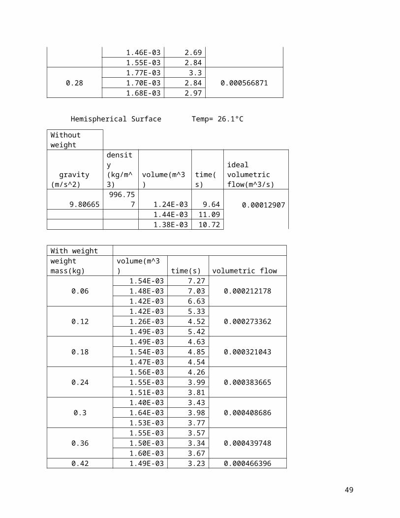
Hemispherical Surface Temp= 26.1°C
Without weight
gravity (m/s^2)density (kg/m^3) volume(m^3) time(s)
ideal volumetric flow(m^3/s)
9.80665 996.757 1.24E-03 9.64 0.00012907
1.44E-03 11.09 1.38E-03 10.72
With weightweight mass(kg) volume(m^3) time(s) volumetric flow
0.061.54E-03 7.27
0.0002121781.48E-03 7.031.42E-03 6.63
38

0.121.42E-03 5.33
0.0002733621.26E-03 4.521.49E-03 5.42
0.181.49E-03 4.63
0.0003210431.54E-03 4.851.47E-03 4.54
0.241.56E-03 4.26
0.0003836651.55E-03 3.991.51E-03 3.81
0.31.40E-03 3.43
0.0004086861.64E-03 3.981.53E-03 3.77
0.361.55E-03 3.57
0.0004397481.50E-03 3.341.60E-03 3.67
0.421.49E-03 3.23
0.0004663961.64E-03 3.621.76E-03 3.63
0.481.60E-03 3.22
0.0004911731.65E-03 3.311.64E-03 3.43
Orifice Steady State
volume (m^3) time (s) Q(m^3/s) h (m) x(m) y (m)
6.30E-04 40.58 1.55773E-05
0.35306
0.053975 05.80E-04 37.07 0.0762 0.002545.70E-04 36.63 0.1016 0.00508
0.127 0.008890.1524 0.013970.1778 0.019304
3.25E-04 22.36 0.3048
0.05715 0.0009653.10E-04 21.36 0.08255 0.00508
39

1.46307E-05
3.00E-04 20.21 0.1143 0.0111760.14605 0.016764
0.1778 0.025908
0.2032 0.0323853.20E-04 23.83
1.34904E-05
0.25654
0.0555625 0.0043183.10E-04 23.01 0.0762 0.0062992.90E-04 21.37 0.1016 0.01016
0.127 0.0173990.1524 0.0246380.1778 0.032639
Orifice- Unsteady State
Weir Trial 1
volume (m^3) time (s) volumetric flow (m^3/s) H(m) H(m) half of weir
1.60E-03 2.65.86E-04 0.045847 0.05081.74E-03 3.1
1.81E-03 3.111.44E-03 2.94
5.05E-04 0.0419862 0.046991.29E-03 2.471.49E-03 2.961.40E-03 3.53
4.02E-04 0.0343408 0.03811.61E-03 3.971.60E-03 3.971.52E-03 6.83 2.18E-04 0.02413 0.0254
h (m) t (s)0.3556 00.3429 29.280.3302 61.120.3175 91.840.3048 122.630.2921 153.780.2794 185.130.2667 217.89
0.254 253.930.2413 289.38
40

1.54E-03 7.191.47E-03 6.774.70E-04 18.19
2.51E-05 0.00889 0.0090176.55E-04 26.214.70E-04 19.09
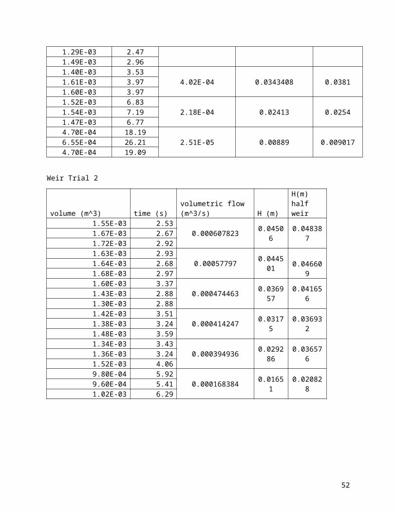
Weir Trial 2
volume (m^3) time (s) volumetric flow (m^3/s) H (m)H(m) half weir
1.55E-03 2.530.000607823 0.04506 0.0483871.67E-03 2.67
1.72E-03 2.921.63E-03 2.93
0.00057797 0.0445010.046609
1.64E-03 2.681.68E-03 2.971.60E-03 3.37
0.000474463 0.036957 0.0416561.43E-03 2.881.30E-03 2.881.42E-03 3.51
0.000414247 0.03175 0.0369321.38E-03 3.241.48E-03 3.591.34E-03 3.43
0.000394936 0.029286 0.0365761.36E-03 3.241.52E-03 4.069.80E-04 5.92
0.000168384 0.01651 0.0208289.60E-04 5.411.02E-03 6.29
Sample Calculations
Jet Impact (Plane target)
For the sample calculations of the Jet Impact (Plane target) experiment, information from Table
2 was used regarding the first trial of experimentation. In order to obtain the experimental slope,
the impacted area must be calculated. The assumption that the diameter of the jet is the same as
that of the nozzle all the way through must be made to achieve this. The diameter of the nozzle is
0.01m.
Table 1: Data Used for Sample Calculations
Second trial
41

26.5°C
Weight: 0kg
V (m3) t (s)
0.00144 12.54
0.00165 14.4
0.00174 15.16
Weight: 0.28kg
V (m3) t (s)
0.00184 3.36
0.00179 3.57
0.00183 3.6
The following sample calculations will be performed using data from Table 10, which is taken
from table 2.
- Initial volumetric flow rate (with 0kg) is obtained dividing the volume inside a calibrated
cylinder by the time it took to fill that volume:
- Volumetric flow rate (with 0.28kg) is obtained the same way as the previous step with the
only difference being that there is more weight added:
- Squared volumetric flow rate difference is obtained squaring the volumetric flow rate at
all the different weights and subtracting the squared initial flow rate:
Results for all weights are shown in Table 11:
42

Table 2: Flow Difference for all Weights
mp
Q2-Qi2
0.035 3.9E-08
0.070 6.53E-08
0.105 7.71E-08
0.140 1.05E-07
0.175 1.61E-07
0.210 1.81E-07
0.245 2.3E-07
0.280 2.56E-07
- Theoretical Slope:
Density of water at 26.5°C was obtained from Table 2-28 of Perry’s Chemical Engineers’
Handbook. The gravity of Earth, g, was obtained from Appendix F.2 of BSL’s book.
The percent error between the experimental and the theoretical slope was calculated as follows:
43
Flow through orifice (Steady State)
Values of height on the x and y directions were obtained. The values used to perform all
calculations were obtained from flow through orifice first trial. The values of the x and y
direction was obtained in inches; the conversion to meter is (1 in = 0.0254 m), the calculation is:
- For the plot of vs. (y)
Calculation of
Graphs of vs. y were constructed in order to calculate the experimental velocity
coefficient (Figure 31). Again, linear regressions were made to each graph.
Table 12 shows the data for the height of 0.353m.
Table 3: Experimental Data for a height of 0.353m
x2/h (m) y (m)
0.008251574 0
0.016446043 0.00254
0.02923741 0.00508
0.045683453 0.00889
0.065784173 0.01397
0.089539568 0.019304
44

Figure 31: Flow through an Orifice for h=0.381 (m)
From Figure 21 the value of the slope is:
The calculation of the velocity coefficient is performed by the following equation:
The theoretical value of the velocity coefficient is 0.98
The error percentage for the velocity coefficient was calculated
A volumetric flow rate value was calculated for three different heights. For the height of
13.9 in, the following volumetric flow rate was obtained:
Calculation of
45
errorthCv
thCvCv %100)(
)((exp)
%73.5100980.0
980.0036.1

Graphs of Q2 vs. h (m) were constructed in order to calculate the experimental discharge
coefficient. Again linear regressions are made.
Table 4: Volumetric flow rate data for Steady State
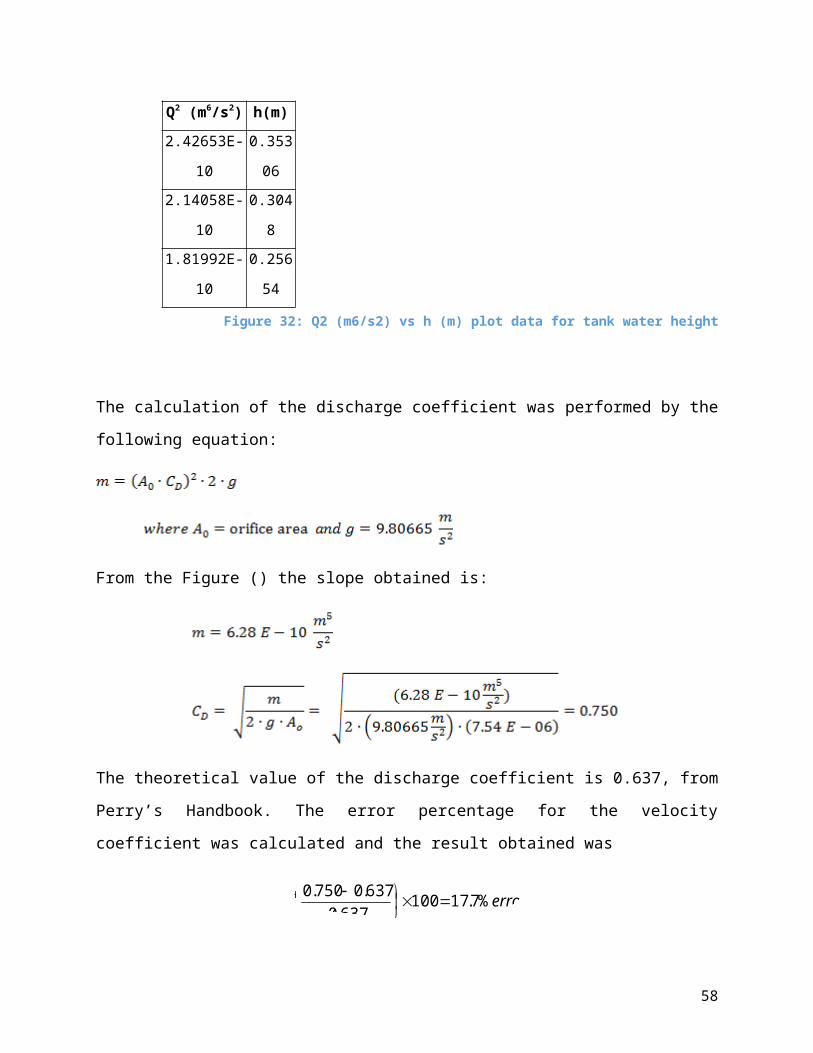
Figure 32: Q2 (m6/s2) vs h (m) plot data for tank water height
The calculation of the discharge coefficient was performed by the following equation:
From the Figure () the slope obtained is:
Q2 (m6/s2) h(m)
2.42653E-10 0.35306
2.14058E-10 0.3048
1.81992E-10 0.25654
46

The theoretical value of the discharge coefficient is 0.637, from Perry’s Handbook. The error
percentage for the velocity coefficient was calculated and the result obtained was
Flow through orifice (Unsteady State)
The heights inside the tank were measured in inches and
the conversion to meters is the same as steady state. The result in meter was 0.3556 m.
Calculating , where h1 = 0.3556 m and is the reference height
Table 5: Data for determination of CD
h (m)(h1
1/2-h1/2)
Time
(s)
0.3556 0 0
0.3429 0.010745422 29.28
0.3302 0.021691745 61.12
0.3175 0.032850677 91.84
0.3048 0.044235111 122.63
0.2921 0.055859296 153.78
0.2794 0.067739049 185.13
0.2667 0.079892007 217.89
0.254 0.092337934 253.93
0.2413 0.105099097 289.38
47
error%7.17100637.0
637.0750.0

Figure 33: Flow through an orifice (Unsteady State)
A graph of t (s) vs. was constructed in order to calculate the experimental
discharge coefficient see figure ( ). The slope obtained is:
The slope is defined as:
AR is the reservoir area, which is calculated as follows:
Tank Length= 0.283 m and tank Width= 0.127 m
Solving for CD:
48
The theoretical value of the discharge coefficient is 0.637.The error percentage for the velocity
coefficient was calculated as previous parts and the result obtained was 18.91%.
Flow through a rectangular Weir
The height values were measured in inches. A conversion was performed to obtain all
values with meters units as follows:
0.0458 m
Calculation of :
A graph of Q (m3/s) vs. was constructed in order to obtain a linear regression equation
(Figure)
Table 6: Data for the determination of CD
Figure 34: Plot of Q vs H3/2 for different positions.
Q (m3/s)H3/2
(opening)
H3/2
(middle)
5.86E-04 0.0098 0.0114
5.05-05 0.0086 0.0101
4.02-04 0.0063 0.0074
2.18E-04 0.0037 0.0040
2.51E-05 0.0008 0.0008
49

From Figure the slope obtained for the H(3/2) opening is:
Solving for CD
The theoretical value of the discharge coefficient is 0.6 obtained from the Perry’s Handbook.
The error percentage for the velocity coefficient was calculated as previous parts and the result
was 16.66%.
50

Results
Jet ImpactThe jet impact experiment consisted of a jet hitting two different targets: a plane and a
hemispherical one.
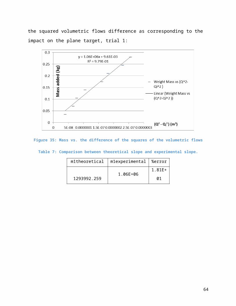
Plane TargetFor the first trial, several weights were placed in order to manipulate the flow and thus
counteract the weight. The following graph illustrates the linear relationship between the weight
and the squared volumetric flows difference as corresponding to the impact on the plane target,
trial 1:
Figure 35: Mass vs. the difference of the squares of the volumetric flows
Table 7: Comparison between theoretical slope and experimental slope.
m1theoretical m1experimental %error
1293992.259 1.06E+06 1.81E+01
51
Hemispherical TargetWhile for the hemispherical target the behavior, which requires more weight to counteract the jet
force than with the plane target, is the following:
Figure 36: Mass vs. the difference of the squares of the volumetric flows
Table 8: Comparison between slopes
m2theoretical m2experimental %error
2587984.519 2.27E+06 1.23E+01
While, for the second trial, the respective behaviors for the plane and hemispherical
targets:
52

Figure 37: Mass vs. the difference of the squares of the volumetric flows: plane target.
Table 9: Comparison between slopes
m1theoretical m1experimental Error %
1293992.259 886296 31.51
Figure 38: Mass vs. the difference of the squares of the volumetric flows
Table 10: Comparison between slopes
m2theoretical m2experimental %error
2588264.961 2.10E+06 18.86
53

Flow through Orifices
Two methods were applied to this experiment: steady and unsteady state analyses. In the
case of flow through orifices, steady state method, with a constant flow which is varied
thrice:
Figure 39: The three different flows selected for the orifice experiment vs. height.
Table 11: Squared horizontal distance vs. vertical distance
14 in
x^2/h (m) y (m)
0.008251574 0
0.016446043 0.00254
0.02923741 0.00508
0.045683453 0.00889
0.065784173 0.01397
0.089539568 0.019304
12 in
0.010715625 0.000965
0.022357292 0.00508
54

0.0428625 0.011176
0.069982292 0.016764
0.103716667 0.025908
0.135466667 0.032385
10 in
0.012033957 0.004318
0.022633663 0.006299
0.040237624 0.01016
0.062871287 0.017399
0.090534653 0.024638
0.123227723 0.032639
Table 12: Discharge and velocity coefficients per height selected.
m,experimental Cv,experimental Cv,theoretical Error %
T,water
(°C)
4.2946 1.036170835 0.98 5.731718 28.4
Second Height
3.9914 0.998924422 0.98 1.931063 28.4
Third Height
3.814 0.976473246 0.98 0.359873 29.6
Table 13: Squared volumetric flow vs height
Q2 (m6/s2) h (m)
2.42653E-10 0.35306
2.14058E-10 0.3048
1.81992E-10 0.25654
Table 14: Slope, CD, AO, CD, theo, diameter and error percentage
m,experimenta
l Cd,experimental Ao (m2) g (m/s2) Cd,theoretical Diameter (m) Error %
55

6.28E-10 0.750287153 7.5418E-06 9.80665 0.637 0.0030988 17.78448245
Figure 40: Squared horizontal distance vs. vertical distance
Figure 41: Squared horizontal distance vs. vertical distance
56

Figure 42: Squared horizontal distance vs. vertical distance
For the unsteady state method, a specific height was selected and water was let to flow
through the orifice without a flow entering the reservoir. Time was recorded for every
half inch:
Table 15: Difference of squared heights, radius area, CD, exp, CD, theo, slope, error percentage
(h1)1/2 - (h)1/2 Ar (m2) Cd,experimental g (m^2/s) m,experimental Ao Cd,theo %error
0 0.034597 0.757451957 9.80665 2735
7.54E-
06 0.637 18.90926
0.010745422
0.021691745
0.032850677
0.044235111
0.055859296
0.067739049
0.079892007
0.092337934
0.105099097
57
Flow through Rectangular Weirs
Next, the flow through weirs was studied. Data from water heights at the top of the weir
entrance and at half the distance between the weir and the first metallic mesh were
collected in two trials:
A) First Trial
At the top of the weir entrance:
Table 16: Calculated volumetric flows, height and height raised to the (3/2)th power
volumetric flow (m3/s) H (m) Q (m3/s) H3/2 (m3/2)
5.86E-04 0.045847 5.86E-04 0.00981672
5.05E-04 0.0419862 5.05E-04 0.008603197
4.02E-04 0.0343408 4.02E-04 0.006363787
2.18E-04 0.02413 2.18E-04 0.003748314
58
Figure 43: Time vs. difference of squared heights

2.51E-05 0.00889 2.51E-05 0.00083821
Figure 44: Volumetric flow vs. H3/2
Table 17: Error percentage for CD
m,experimental L (m) g (m^2/s) Cd,experimental Cd,theoretical %error
6.20E-02 0.03 9.80665 0.699981171 0.6 16.66353
At half the distance:
Table 18: Volumetric flows and heights
Q (m3/s) H3/2 (m3/2)
0.000585582 0.011449739
0.000505147 0.010186105
0.000401722 0.007436823
0.000217956 0.004048094
2.51497E-05 0.000856235
59
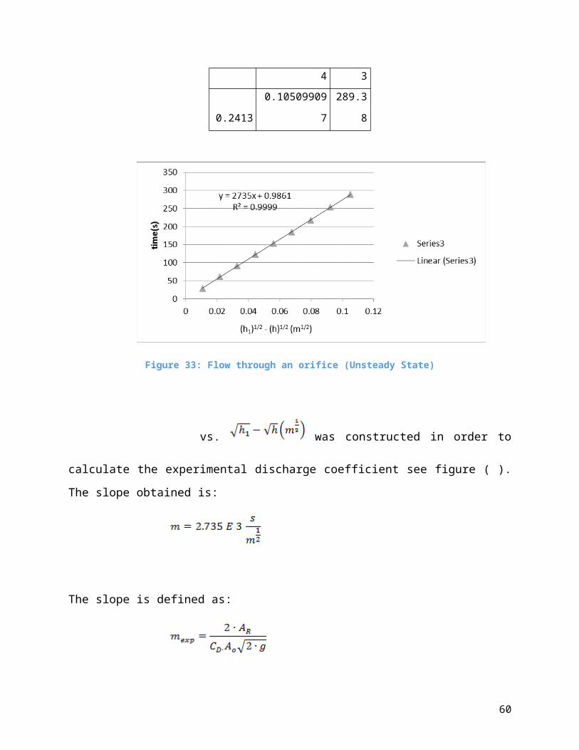
Figure 45: Q (m3/s) vs H3/2 (m3/2)
B) Second Trial
At the top of the weir:
Table 19: Volumetric flows and heights
volumetric flow (m3/s) H (m) Q (m3/s) H3/2 (m3/2)
0.000607823 0.04506 0.000608 0.009564912
0.00057797 0.044501 0.000578 0.009387538
0.000474463 0.036957 0.000474 0.007104689
0.000414247 0.03175 0.000414 0.005657383
0.000394936 0.029286 0.000395 0.005011809
60

0.000168384 0.01651 0.000168 0.00212139
Figure 46: Volumetric flow vs. H3/2
Table 20: Error percentage for CD
m,experimental L (m) g (m2/s) Cd,experimental Cd,theoretical %error
5.50E-02 0.03 9.80665 0.620951039 0.6 3.49184
At half the distance between weir and metallic mesh:
Table 21: Volumetric flows and heights
Q (m3/s) H3/2 (m3/2)
0.000607823 0.01064371
0.00057797 0.010062472
0.000474463 0.008501907
0.000414247 0.007097366
0.000394936 0.006995106
61

0.000168384 0.003005878
Figure 47: Volumetric flow vs. H3/2
Table 22: Error percentage for CD
m,experimental L (m)
g
(m^2/s) Cd,experimental Cd,theoretical %error
5.74E-02 0.028575 9.80665 0.680364393 0.6 13.39406553
62

Discussion of ResultsResults from Hydraulic Bench experiments verified Newton’s Second Law of Mass and
Momentum Conservation for different geometries. Starting with the Jet Impact experiment in
which the water force exerted against targets of different geometries was studied. It was
observed that the hemispherical target could withstand a larger amount of weight with a similar
flow to the flat target. From the experimental data for both targets it can be observed that for
both trials the hemispherical target has about twice the value of the plane target, meaning that
twice the force is exerted. This behavior confirms the theoretical equations. The ratio between
slopes is 2 for the theoretical values and 2.14 for the experimental values. The error percentages
obtained were in the range 18.1% and 31.51% for the plane target for the first and second trials,
respectively, and in the range of 18.3% and 18.86% for the first and second trials, respectively,
for the hemispherical target. Discrepancies in values could be due to inability to completely
control equipment, be it the flow or the weights not being evenly distributed on the plate, among
other environmental factor that could have affected. Another possibility that could explain the
fluctuation in the error percentages (the one present in the second trial nearly doubles the first
one) is the efficiency of the pump, which could deliver inconsequent flows from time to time. It
was necessary to perform an additional trial due to the fact that, in a failed trial, the last three
volumetric flows that counteracted the 210, 245 and 280 kg weights were approximately the
same, which contradicts the expected behavior of linearity between weight added and volumetric
flow.
In the orifice experiment the effect of flow rate on the height and horizontal distance
traveled by the stream of water was observed. The greater the flow rate the farther the stream
reached. For steady state conditions a flow was established to maintain a constant height and
three different measures were selected. The outcoming flows from the orifices at the
corresponding heights were studied to determine the velocity coefficient (CV) and coefficient of
discharge (CD). The theoretical CV (0.980) is constant for all conditions but, as it was observed
experimentally, the values ranged from 1.036 to 0.9989 to 0.976, giving error % from 5.73 to
1.93 to 0.36 and had a definite linear behavior with R2 values ranging from 0.999 to 0.9953 to
0.9974. For the CD a 17.78% error was observed and an R2 value of 0.999 in the linear
relationship between the squared volumetric flows versus the measured height. Most of the error
of this experiment might come from the Vernier scale which was used to measure the positions
63
for the stream, it was loosely positioned over a pair of rails on the equipment and this caused the
human error in the measurements to be significant, which an attempt to diminish it by placing
some masking tape on the rails was done; in addition the pump constantly had a vibration that
was felt through the equipment and might have affected the precision of the test. For the
unsteady part of the experiment the tank was filled to 14 inches and the incoming flow was
ceased. While the level of the tank decreased by, approximately, every 0.5 inches, time was
recorded. Utilizing the slope to determine the CD, a value of 0.757 was observed with an 18.91%
error as compared to the theoretical data.
In the rectangular weir experimentation the relationship between the height of the water
before the weir and the flow above the weir was studied. Two positions of measuring the height
were compared: the first, just above the weir opening and, the second, at half the distance
between the weir and the first metallic mesh whose purpose is to eliminate turbulence in the
equipment. The experimentation was done twice and the error percentages for both trials were,
for the two distances (top of weir and half the distance between the weir and the first metallic
mesh, respectively), 16.66 and 3.49, and, 2.13 and 13.39 %.
64

Conclusions and Recommendations The different principles involving fluids were investigated in the experiment. There were
three separate apparatus used to observe various properties of fluids. Jet impact was used to
determine the weight that force that water had to make in order to withstand some weight. Flow
through orifice studied the various coefficients which affect the ideality of a fluid going through
a orifice. Flow over weir demonstrated the same coefficients but observing how water behavior
changed when passing over a weir. All of these experiments were compared with the literature
values, the errors of all experiments ranged from 0.36% to 31.51%.
It is important to say that the biggest errors came from the jet impact apparatus, this could
be the consequence of either the apparatus being damaged or the water pump fluctuates in flow,
creating errors in the lectures. With this in mind the recommendations of this experiment would
be to maintain or change the water pump, and add an automatic volumetric meter which will
lower the errors when the data is taken.
65

References
Appendix
66