Banco Central de ChileDocumentos de Trabajo

Central Bank of ChileWorking Papers

N° 128

Noviembre 2001

PRICE INFLATION AND EXCHANGE RATEPASS-THROUGH IN CHILE

Carlos José García Jorge Enrique Restrepo

La serie de Documentos de Trabajo en versión PDF puede obtenerse gratis en la dirección electrónica:http://www.bcentral.cl/Estudios/DTBC/doctrab.htm. Existe la posibilidad de solicitar una copiaimpresa con un costo de $500 si es dentro de Chile y US$12 si es para fuera de Chile. Las solicitudes sepueden hacer por fax: (56-2) 6702231 o a través de correo electrónico: bcch@condor.bcentral.cl

Working Papers in PDF format can be downloaded free of charge from:http://www.bcentral.cl/Estudios/DTBC/doctrab.htm. Printed versions can be ordered individually forUS$12 per copy (for orders inside Chile the charge is Ch$500.) Orders can be placed by fax: (56-2) 6702231or e-mail: bcch@condor.bcentral.cl.

BANCO CENTRAL DE CHILE

CENTRAL BANK OF CHILE

La serie Documentos de Trabajo es una publicación del Banco Central de Chile que divulgalos trabajos de investigación económica realizados por profesionales de esta institución oencargados por ella a terceros. El objetivo de la serie es aportar al debate de tópicosrelevantes y presentar nuevos enfoques en el análisis de los mismos. La difusión de losDocumentos de Trabajo sólo intenta facilitar el intercambio de ideas y dar a conocerinvestigaciones, con carácter preliminar, para su discusión y comentarios.

La publicación de los Documentos de Trabajo no está sujeta a la aprobación previa de losmiembros del Consejo del Banco Central de Chile. Tanto el contenido de los Documentosde Trabajo, como también los análisis y conclusiones que de ellos se deriven, son deexclusiva responsabilidad de su(s) autor(es) y no reflejan necesariamente la opinión delBanco Central de Chile o de sus Consejeros.

The Working Papers series of the Central Bank of Chile disseminates economic researchconducted by Central Bank staff or third parties under the sponsorship of the Bank. Thepurpose of the series is to contribute to the discussion of relevant issues and develop newanalytical or empirical approaches in their analysis. The only aim of the Working Papers isto disseminate preliminary research for its discussion and comments.

Publication of Working Papers is not subject to previous approval by the members of theBoard of the Central Bank. The views and conclusions presented in the papers areexclusively those of the author(s) and do not necessarily reflect the position of the CentralBank of Chile or of the Board members.

Documentos de Trabajo del Banco Central de ChileWorking Papers of the Central Bank of Chile

Huérfanos 1175, primer piso.Teléfono: (56-2) 6702475 Fax: (56-2) 6702231

Documento de Trabajo Working PaperN° 128 N° 128

PRICE INFLATION AND EXCHANGE RATEPASS-THROUGH IN CHILE

Carlos José García Jorge Enrique RestrepoEconomista Senior Economista Senior

Gerencia de Análisis Macroeconómico Gerencia de Análisis MacroeconómicoBanco Central de Chile Banco Central de Chile

ResumenEn este trabajo se estimó una ecuación de precios, con datos de Chile entre 1986:1 y 2001:1,derivada de un modelo de competencia imperfecta. La estimación incluye la primera diferencia dela variable dependiente como lo hace la literatura acerca de la estimación de modelos de costos deajuste lineales cuadráticos cuando la variable objetivo y algunas de las variables que mueven elproceso son procesos I(2). La ecuación se usa para generar proyecciones fuera de muestra de uníndice de precios más restringido que el IPC. De los resultados podemos concluir: i) el traspaso detipo de cambio a precios depende positivamente de la actividad económica (brecha del producto) loque explica por qué el traspaso a precios ha sido tan bajo en los últimos años en Chile. En otraspalabras una brecha del producto negativa ha compensado el impacto inflacionario de ladepreciación del peso; ii) la productividad reduce los costos laborales unitarios y la inflación; iii)salarios y precios externos están relacionados positivamente con la inflación; iv) finalmente, laaceleración de la inflación esperada es una variable significativa en el modelo, lo que confirma quelas expectativas importan en la determinación de la inflación.

AbstractA price equation based on a model of imperfect competition was estimated using quarterly data forChile from 1986:1 to 2001:1. The estimation includes the first difference of the dependent variablefollowing the literature on the estimation of linear quadratic adjustment cost (LQAC) models, whenthe target and some of the driving variables follow I(2) processes. The equation is used to generateout-of-sample inflation forecast, of a narrower-than the-CPI price index. We can conclude from theestimation results: i) exchange-rate pass-through depends positively on economic activity (outputgap) explaining why pass-through has been so low in recent years in Chile. In other words, anegative output gap has compensated the inflationary impact of exchange-rate depreciation; ii)productivity reduces unit labor costs and inflation; iii) wages and foreign prices are positivelyrelated to inflation; iv) Finally, expected inflation acceleration is significant, confirming thatexpectations matter determining inflation.

____________________The views expressed in this paper are those of the authors and should not be attributed to the Central Bank ofChile. We would like to thank Francisco Figueiredo, Pablo García, Esteban Jadresic, Leonardo Luna, CarlosEsteban Posada, Rodrigo Valdés, two anonymous readers and seminar participants at the Central Bank ofChile, the Bank of International Settlements, CEA-Universidad de Chile, and the VI CEMLA central banksmeeting, for their comments and suggestions. E-mails: cgarcia@bcentral.cl ; jrestrep@bcentral.cl.

1

I. Overview

This article estimates a price equation using quarterly Chilean data from 1986:1 to

2001:1. Several issues that are important for understanding and anticipating the behavior

of inflation could motivate the estimation of such an equation. For instance: i) elasticity

of inflation to the output gap ii) the permanent and cyclical movements of mark-ups, iii)

effects of labor productivity growth on inflation, iv) credibility and v) the size of the

exchange rate pass-through.

Even though the estimation is related to all these subjects, we take a closer look at the

pass-through effect, defined as the effect of exchange-rate changes on domestic inflation,

because apparently, this factor has substantially changed in recent years1. The exchange

rate pass-through has been low recently despite the fact that Chile is a small open

economy. In fact, there has been significant peso depreciation since 1997 without having

a strong impact on inflation. Why is this? Is a low pass-through a new permanent

characteristic of the Chilean economy? Will depreciation’s impact on inflation take place

as soon as demand takes off again? The answer to these questions is crucial for defining

monetary policy. The international evidence shows that a very low exchange-rate pass-

through has also been observed in New Zealand, Brazil and Australia, where substantial

depreciation has taken place after 1997 without having a proportional effect on inflation2.

In general, the exchange rate affects the price of any tradable good3. However, the most

important channel for passing depreciation to inflation is the direct short-term effect of

the exchange rate on the imported part of the basket of goods that make up the CPI and

the imported inputs. The larger the share of imported goods within the CPI basket, the

greater the exchange rate effect on prices. In Chile, about 48% of CPI goods are

1 We compute it here as the ratio between accumulated inflation and accumulated depreciation after a shockhas hit the last variable.2 There has been a great amount of articles written on pass-through over the years. For a survey see Golbergand Knetter (1997). Most of them try to estimate how much exchange rate fluctuations are responsible forthe behavior of inflation. Some use CPI inflation others use producer price inflation. There is also a widerange of estimation techniques used to obtain a quantitative result. It goes from ordinary least squares (Woo1984), to panel data (De Gregorio and Borensztein (1999), Goldfajn and Werlang 2000), vector autoregression (McCarthy 1999), cointegration analysis and error correction models (Beaumont et al 1994, KimK. 1998, Kim Y. 1990), and state-space models (Kim Y. 1990).

2

considered importable. The exchange rate also directly affects the cost structure of

companies using imported inputs. Thus, the greater the proportion of imported inputs

making up the costs, the more depreciation will affect these companies’ prices. It is

important to note that we have considered in our estimation a narrower definition of

prices than CPI, which we call core inflation throughout the paper4.

Monetary policy and agents’ expectations also influence the effect on prices of

exchange–rate depreciation. Although in the short-term, inflation may rise due to

depreciation, in the medium– and long–term, inflation should fall back to the target or

range level defined by the Central Bank. Of course, an active monetary policy implies

affecting aggregate demand and the exchange rate itself5.

Phillips curves have been estimated for Chile before (García, Herrera, and Valdés 2000).

Nonetheless, we will follow a different approach here. Instead of estimating a reduced

form relation between the change in inflation and the output gap, we will estimate an

equation for price inflation that considers explicitly a model of nominal price setting by

imperfect competitive firms. In addition, we use the linear quadratic price adjustment cost

model (LQAC) in Rotemberg (1982), where the representative firm chooses a sequence

of prices for solving its intertemporal problem. As a result, inflation can be represented as

an error correction equation (Euler equation), relating this variable to expected inflation

as well as to the gap between the “equilibrium” and actual price level. The error

correction in the price equation ensures that in the steady state, the price level is a mark-

up on unit labor costs. Different versions of the core–price equation are estimated by

using a single–equation error correction procedure.

Moreover, an I(2) analysis of inflation and the mark-up is undertaken. We find that the

price level is best described as an I(2) process. It is worth stressing that Chile is not an

3 The exchange rate effect on prices of exportables is empirically less important given that some of Chile’smain exports are not included in the core price index, like: fruits, or even in the CPI like: copper, fishmeal,wood pulp, salmon, methanol, etc.4 The price index is around 70% of CPI because we took out perishable goods and regulated services.Therefore, our estimation of the pass-through coefficient should be taken carefully, since some regulatedservices are very sensitive to changes in the exchange rate.5 Another factor affecting the degree of pass-through is how permanent agents perceive the shock. We willnot deal with exchange-rate volatility here, though.

3

exception in this regard. In fact, Roberts (2001) models inflation as a unit–root process

for the USA. Johansen (1992) and Engstead and Haldrup (1999) do the same for UK.

Barnerjee, Cockerell and Russell (2001) find that prices in Australia are better described

as an I(2) process as well. In order to deal with I(2) processes, we incorporate inflation as

an additional component of the “equilibrium” price in the Euler equation (Engsted and

Haldrup 1999; Barnerjee, et al. 2001). On the other hand, we deal with the inflation

expectation term using the limited-information approach due to McCallum (1976).

Taking the estimated price equation, the exchange-rate pass-through is analyzed by

simulating an exchange rate shock, with and without an output gap since pass-through is

related to economic activity, but also with and without full wage indexation. Had a

negative output gap not existed after 1997, the exchange–rate effect on inflation would

have been significantly higher. In addition, as a consequence of prices being positively

related to wages, the simulation shows that when wage indexation is not complete –and

wages grow less than past inflation– pass-through is lower in the long run. The results

also show, as expected, that labor productivity reduces unit labor costs and inflation.

This article is organized as follows. The second section introduces some preliminary

evidence on the recent pass-through reduction and presents a price model. The third

section presents the estimation results and the pass-through simulation. Finally there are

some conclusions.

II. Pass-Through from Depreciation to Inflation

a. Stylized facts

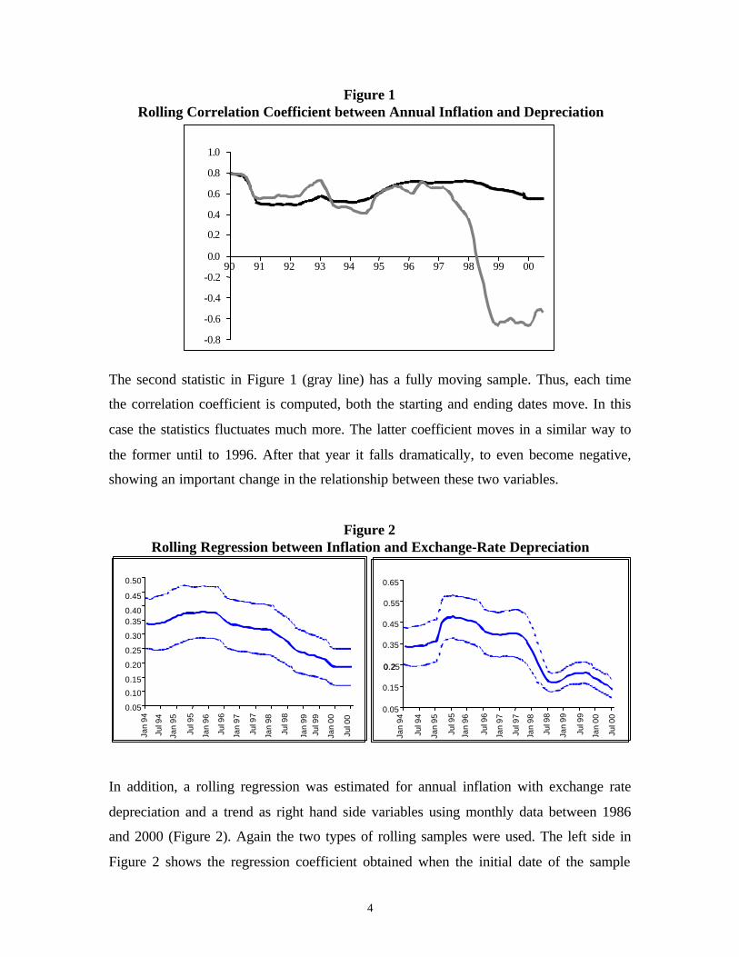
The simplest exercise one can realize regarding the pass-through is to compute the

correlation between inflation and exchange–rate depreciation. In this case, two rolling

correlation statistics were computed (Figure 1). The first one (dark line) has its starting

date fixed (1986:1) and the correlation coefficient is calculated adding a new observation

at a time, starting in 1990. Therefore, each computation has a larger sample than the last

one. Even though this coefficient is rather stable, it has some movement. It decreases at

the beginning of the nineties, grows again from 1994 to 1996 and falls steadily after

1998.

4

Figure 1Rolling Correlation Coefficient between Annual Inflation and Depreciation

-0.8

-0.6

-0.4

-0.2

0.0

0.2

0.4

0.6

0.8

1.0

90 91 92 93 94 95 96 97 98 99 00

The second statistic in Figure 1 (gray line) has a fully moving sample. Thus, each time

the correlation coefficient is computed, both the starting and ending dates move. In this

case the statistics fluctuates much more. The latter coefficient moves in a similar way to

the former until to 1996. After that year it falls dramatically, to even become negative,

showing an important change in the relationship between these two variables.

Figure 2Rolling Regression between Inflation and Exchange-Rate Depreciation

0.05

0.15

0.25

0.35

0.45

0.55

0.65

0.05

0.10

0.15

0.20

0.25

00.35

0.350.40

0.45

0.50

Jan

94

Jul 9

4

Jan

95

Jul 9

5

Jan

96

Jul 9

6

Jan

97

Jul 9

7

Jan

98

Jul 9

8

Jul 9

9

Jan

00

Jul 0

0

0.30

0.25

0.20

0.15

0.10

0.05

Jan

94

Jul 9

4

Jan

95

Jul 9

5

Jan

96

Jul 9

6

Jan

97

Jul 9

7

Jan

98

Jul 9

8

Jan

99

Jan

99

Jul 9

9

Jan

00

Jul 0

0

0.65

0.55

0.45

0.35

0.250.2

0.15

0.05

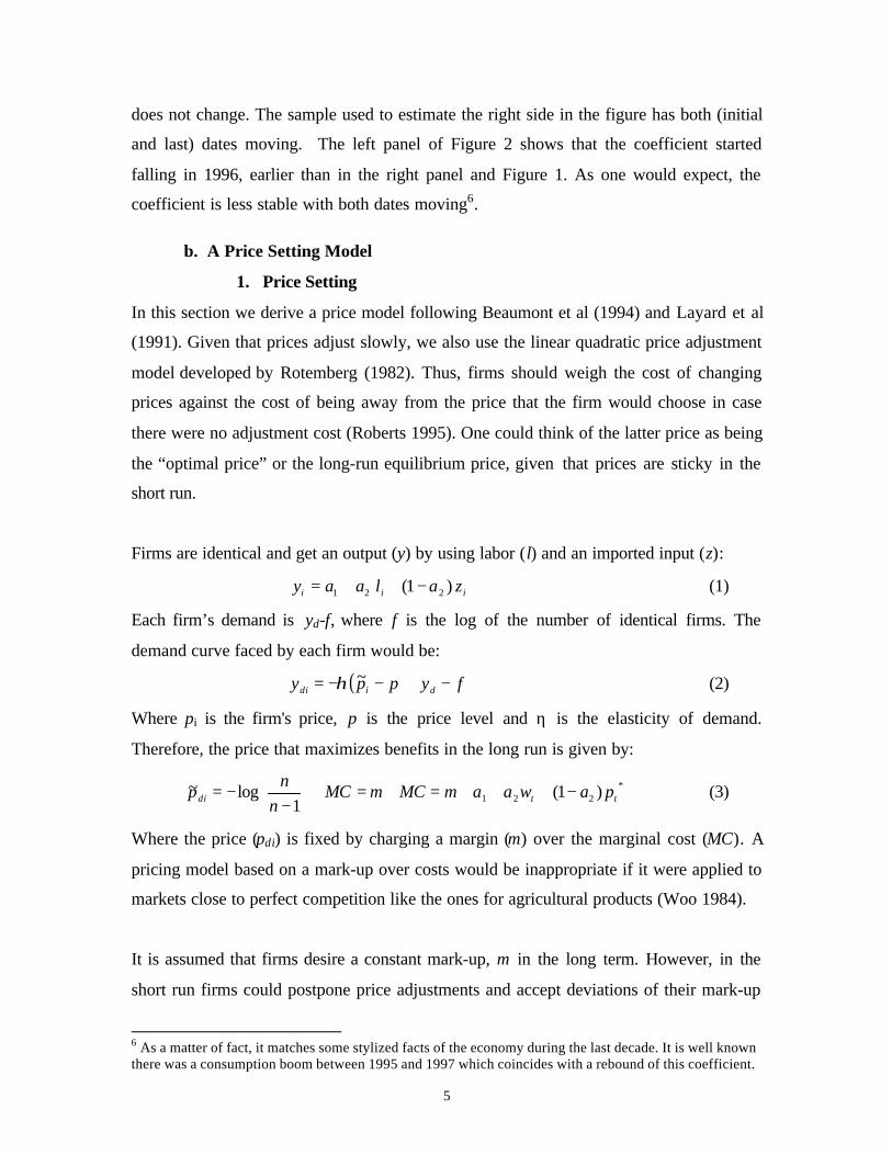
In addition, a rolling regression was estimated for annual inflation with exchange rate

depreciation and a trend as right hand side variables using monthly data between 1986

and 2000 (Figure 2). Again the two types of rolling samples were used. The left side in

Figure 2 shows the regression coefficient obtained when the initial date of the sample

5

does not change. The sample used to estimate the right side in the figure has both (initial

and last) dates moving. The left panel of Figure 2 shows that the coefficient started

falling in 1996, earlier than in the right panel and Figure 1. As one would expect, the

coefficient is less stable with both dates moving6.

b. A Price Setting Model

1. Price Setting

In this section we derive a price model following Beaumont et al (1994) and Layard et al

(1991). Given that prices adjust slowly, we also use the linear quadratic price adjustment

model developed by Rotemberg (1982). Thus, firms should weigh the cost of changing

prices against the cost of being away from the price that the firm would choose in case

there were no adjustment cost (Roberts 1995). One could think of the latter price as being

the “optimal price” or the long-run equilibrium price, given that prices are sticky in the

short run.

Firms are identical and get an output (y) by using labor (l) and an imported input (z):

iii zalaay )1( 221 −++= (1)

Each firm’s demand is yd-f, where f is the log of the number of identical firms. The

demand curve faced by each firm would be:

( ) fyppy didi −+−−= ~η (2)

Where pi is the firm's price, p is the price level and η is the elasticity of demand.

Therefore, the price that maximizes benefits in the long run is given by:

*221 )1(

1log~

ttdi pawaamMCmMCn

np −+++=+=+

−−= (3)

Where the price (pdi) is fixed by charging a margin (m) over the marginal cost (MC). A

pricing model based on a mark-up over costs would be inappropriate if it were applied to

markets close to perfect competition like the ones for agricultural products (Woo 1984).

It is assumed that firms desire a constant mark-up, m in the long term. However, in the

short run firms could postpone price adjustments and accept deviations of their mark-up

6 As a matter of fact, it matches some stylized facts of the economy during the last decade. It is well knownthere was a consumption boom between 1995 and 1997 which coincides with a rebound of this coefficient.

6

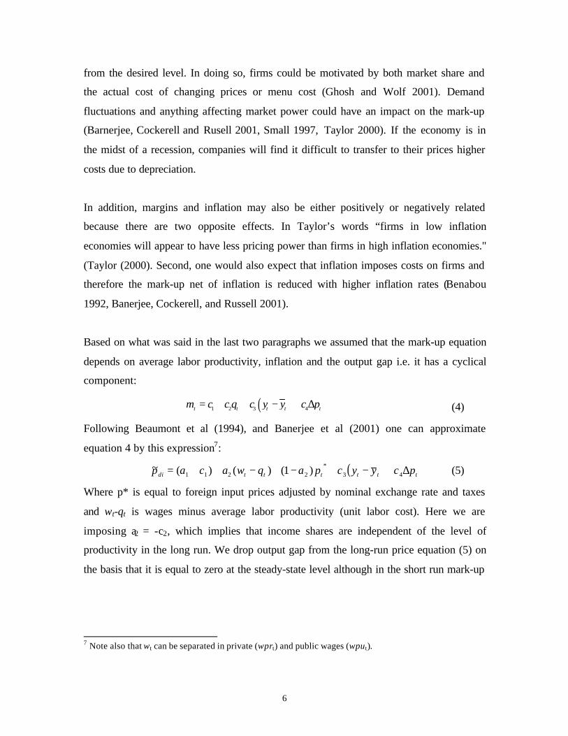
from the desired level. In doing so, firms could be motivated by both market share and

the actual cost of changing prices or menu cost (Ghosh and Wolf 2001). Demand

fluctuations and anything affecting market power could have an impact on the mark-up

(Barnerjee, Cockerell and Rusell 2001, Small 1997, Taylor 2000). If the economy is in

the midst of a recession, companies will find it difficult to transfer to their prices higher

costs due to depreciation.

In addition, margins and inflation may also be either positively or negatively related

because there are two opposite effects. In Taylor’s words “firms in low inflation

economies will appear to have less pricing power than firms in high inflation economies."

(Taylor (2000). Second, one would also expect that inflation imposes costs on firms and

therefore the mark-up net of inflation is reduced with higher inflation rates (Benabou

1992, Banerjee, Cockerell, and Russell 2001).

Based on what was said in the last two paragraphs we assumed that the mark-up equation

depends on average labor productivity, inflation and the output gap i.e. it has a cyclical

component:

( )1 2 3 4t t t t tm c c q c y y c p= + + − + ∆ (4)

Following Beaumont et al (1994), and Banerjee et al (2001) one can approximate

equation 4 by this expression7:

( ) ttttttdi pcyycpaqwacap ∆+−+−+−++= 43

*

2211 )1()()(~ (5)

Where p* is equal to foreign input prices adjusted by nominal exchange rate and taxes

and wt-qt is wages minus average labor productivity (unit labor cost). Here we are

imposing a2 = -c2, which implies that income shares are independent of the level of

productivity in the long run. We drop output gap from the long-run price equation (5) on

the basis that it is equal to zero at the steady-state level although in the short run mark-up

7 Note also that wt can be separated in private (wprt) and public wages (wput).

7

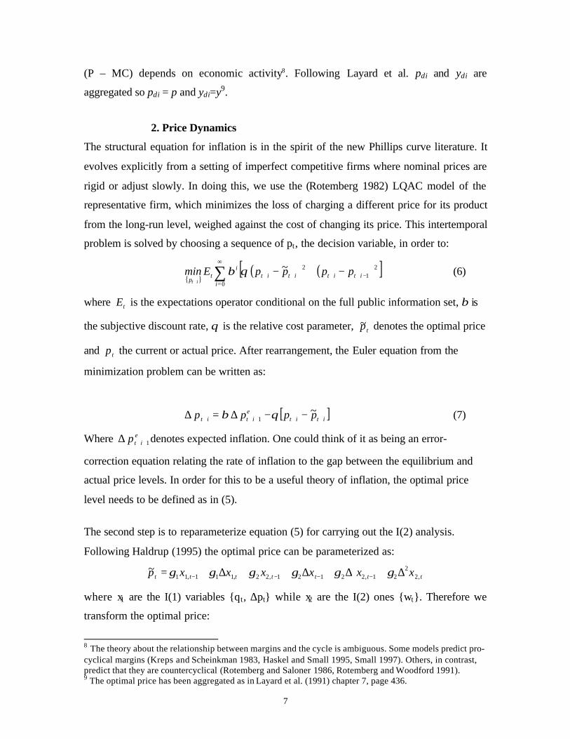
(P – MC) depends on economic activity8. Following Layard et al. pdi and ydi are

aggregated so pdi = p and ydi=y9.

2. Price Dynamics

The structural equation for inflation is in the spirit of the new Phillips curve literature. It

evolves explicitly from a setting of imperfect competitive firms where nominal prices are

rigid or adjust slowly. In doing this, we use the (Rotemberg 1982) LQAC model of the

representative firm, which minimizes the loss of charging a different price for its product

from the long-run level, weighed against the cost of changing its price. This intertemporal

problem is solved by choosing a sequence of pt, the decision variable, in order to:

{ }( ) ( )[ ]2

12

0

~−++++

∞

=

−+−∑+

ititititi

it

pppppEmin

it

θβ (6)

where tE is the expectations operator conditional on the full public information set, β is

the subjective discount rate, θ is the relative cost parameter, tp~ denotes the optimal price

and tp the current or actual price. After rearrangement, the Euler equation from the

minimization problem can be written as:

[ ]itite

itit pppp +++++ −−∆=∆ ~1 θβ (7)

Where eitp 1++∆ denotes expected inflation. One could think of it as being an error-

correction equation relating the rate of inflation to the gap between the equilibrium and

actual price levels. In order for this to be a useful theory of inflation, the optimal price

level needs to be defined as in (5).

The second step is to reparameterize equation (5) for carrying out the I(2) analysis.

Following Haldrup (1995) the optimal price can be parameterized as:

ttttttt xxxxxxp ,22

21,22121,22,111,11~ ∆+∆+∆++∆+= −−−− γγγγγγ

where x1 are the I(1) variables {qt, ∆pt} while x2 are the I(2) ones {wt}. Therefore we

transform the optimal price:

8 The theory about the relationship between margins and the cycle is ambiguous. Some models predict pro-cyclical margins (Kreps and Scheinkman 1983, Haskel and Small 1995, Small 1997). Others, in contrast,predict that they are countercyclical (Rotemberg and Saloner 1986, Rotemberg and Woodford 1991).9 The optimal price has been aggregated as in Layard et al. (1991) chapter 7, page 436.

8

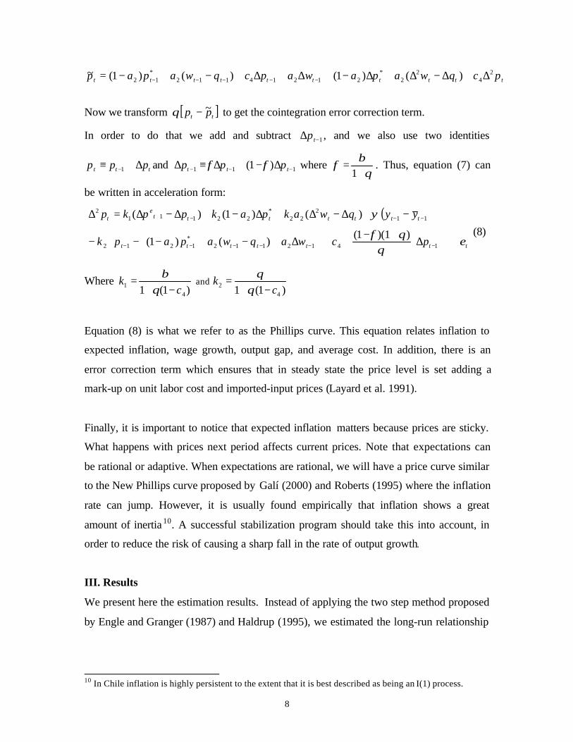
tttttttttt pcqwapawapcqwapap 24

22

*21214112

*12 )()1()()1(~ ∆+∆−∆+∆−+∆+∆+−+−= −−−−−

Now we transform [ ]tt pp ~−θ to get the cointegration error correction term.

In order to do that we add and subtract 1−∆ tp , and we also use two identities

ttt ppp ∆+≡ −1 and 111 )1( −−− ∆−+∆≡∆ ttt ppp φφ where θ

βφ+

=1

. Thus, equation (7) can

be written in acceleration form:

( )

ttttttt

ttttttte

t

pcwaqwapapk

yyqwakpakppkp

εθ

θφ

ψ

+

∆

+−++∆+−+−−−

−+∆−∆+∆−+∆−∆=∆

−−−−−−

−−−+

1412112*

1212

112

22*

221112

)1)(1()()1(

)()1()(

(8)

Where )1(1 4

1 ck

−+=

θβ

and )1(1 4

2 ck

−+=

θθ

Equation (8) is what we refer to as the Phillips curve. This equation relates inflation to

expected inflation, wage growth, output gap, and average cost. In addition, there is an

error correction term which ensures that in steady state the price level is set adding a

mark-up on unit labor cost and imported-input prices (Layard et al. 1991).

Finally, it is important to notice that expected inflation matters because prices are sticky.

What happens with prices next period affects current prices. Note that expectations can

be rational or adaptive. When expectations are rational, we will have a price curve similar

to the New Phillips curve proposed by Galí (2000) and Roberts (1995) where the inflation

rate can jump. However, it is usually found empirically that inflation shows a great

amount of inertia 10. A successful stabilization program should take this into account, in

order to reduce the risk of causing a sharp fall in the rate of output growth.

III. Results

We present here the estimation results. Instead of applying the two step method proposed

by Engle and Granger (1987) and Haldrup (1995), we estimated the long-run relationship

10 In Chile inflation is highly persistent to the extent that it is best described as being an I(1) process.

9

together with the dynamics, as in equation (8), following Harris (1995)11. As this author

puts it, when estimating a long-run equation, superconsistency ensures that it is

asymptotically valid to omit the stationary I(0) terms, however the long-run relationship

estimates will be biased in finite samples (see also Phillips 1986). Therefore, Harris

concludes (citing Inder 1993) that in the case of finite samples, "the unrestricted dynamic

model gives... precise estimates [of long-run parameters] and valid t-statistics, even in the

presence of endogenous explanatory variables" (Harris op.cit., p.p. 60-61). At the same

time it is also possible to test the null hypothesis of no cointegration by testing the

significance of the error correction coefficient (Harris op cit., for an explanation and

critical values see Banerjee, Dolado Galbraith, and Hendry, 1993 p. 223-233).

In addition, an I(2) analysis of inflation and the mark-up is done as in Haldrup (1995).

We find that the levels of prices and unit labor costs are best described as I(2) processes,

this result can probably be accounted for by the existence of an I(1) inflation target

during the1990s. As said above, Chile is not unique in this regard. In fact, Roberts (2001)

models inflation as a unit–root process for the USA. Johansen (1992) and Engstead and

Haldrup (1999) also do the same for UK. Barnerjee, Cockerell and Russell (2001) who

find that prices in Australia are also better described as an I(2) process as well. An I(1)

inflation process is not necessarily inconsistent with inflation targeting, given that the

target was not “stationary.” Furthermore, an I(1) inflation could be allowed to wander

inside a target range. Since in this case there would be an inaction zone, the monetary

policy reaction function would be nonlinear and is called by Orphanides and Wieland

(2000) “inflation zone targeting.” Such a stochastic process is known in the (continuous

time) literature as a Brownian motion with barriers. Although this kind of process is

expected to settle down to a stationary one in the long run, it is not yet the case in the

sample we are considering here12.

11 Harris, R. Cointegration Analysis in Econometric Modelling pp 60-61. See also Phillips and Loretan(1991) for a comparison among several one-step (uniequational) cointegration methods used to estimatelong-run economic equilibria.12 Another alternative would be treating inflation as a stationary process but using a calibratedautoregressive coefficient very close to 1. In this case, inflation would still be very persistent althoughbeing a stationary process. However, it would be a calibration experiment instead of being an econometricestimation.

10

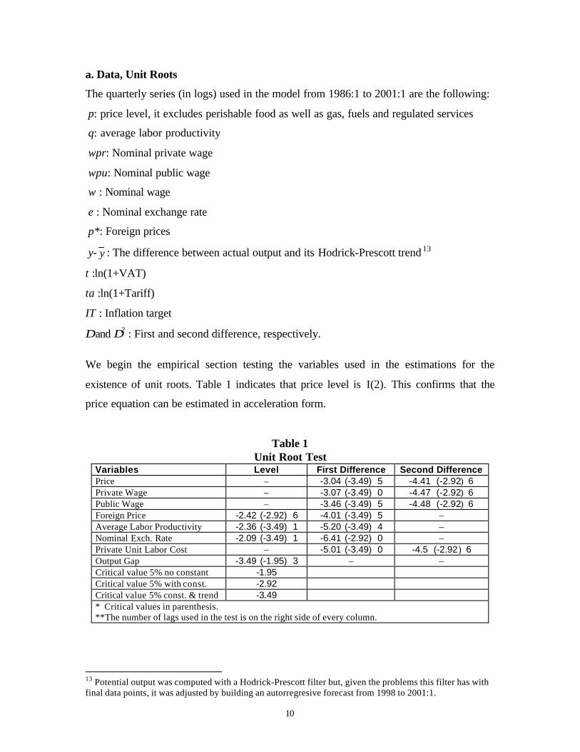
a. Data, Unit Roots

The quarterly series (in logs) used in the model from 1986:1 to 2001:1 are the following:

p: price level, it excludes perishable food as well as gas, fuels and regulated services

q: average labor productivity

wpr: Nominal private wage

wpu: Nominal public wage

w : Nominal wage

e : Nominal exchange rate

p*: Foreign prices

y- y : The difference between actual output and its Hodrick-Prescott trend 13

t :ln(1+VAT)

ta :ln(1+Tariff)

IT : Inflation target

∆ and ∆2 : First and second difference, respectively.

We begin the empirical section testing the variables used in the estimations for the

existence of unit roots. Table 1 indicates that price level is I(2). This confirms that the

price equation can be estimated in acceleration form.

Table 1Unit Root Test

Variables Level First Difference Second DifferencePrice – -3.04 (-3.49) 5 -4.41 (-2.92) 6Private Wage – -3.07 (-3.49) 0 -4.47 (-2.92) 6Public Wage – -3.46 (-3.49) 5 -4.48 (-2.92) 6Foreign Price -2.42 (-2.92) 6 -4.01 (-3.49) 5 –Average Labor Productivity -2.36 (-3.49) 1 -5.20 (-3.49) 4 –Nominal Exch. Rate -2.09 (-3.49) 1 -6.41 (-2.92) 0 –Private Unit Labor Cost – -5.01 (-3.49) 0 -4.5 (-2.92) 6Output Gap -3.49 (-1.95) 3 – –Critical value 5% no constant -1.95Critical value 5% with const. -2.92Critical value 5% const. & trend -3.49* Critical values in parenthesis.**The number of lags used in the test is on the right side of every column.

13 Potential output was computed with a Hodrick-Prescott filter but, given the problems this filter has withfinal data points, it was adjusted by building an autorregresive forecast from 1998 to 2001:1.

11

In general one can say that Chilean inflation deviates from any given mean in the period

here considered. Moreover, Chilean inflation has traditionally been very persistent due to

generalized indexation. On the other hand, variables such as output gap and the nominal

exchange rate are I(0) and I(1) respectively. Regarding cointegration we follow Banerjee,

Dolado Galbraith, and Hendry’s (1993) approach which states that a test of the null

hypothesis Ho: c2 =0 (the error–correction coefficient in equation 8) based on the t-

statistic tk = 0 is a valid test for cointegration. If the variables are not cointegrated, this

coefficient should be zero. They also include computed critical values for this test in

Table 7.6 in their book. Both equations pass the test since the critical t value is 4.06 at 1%

of significance (Table 2).

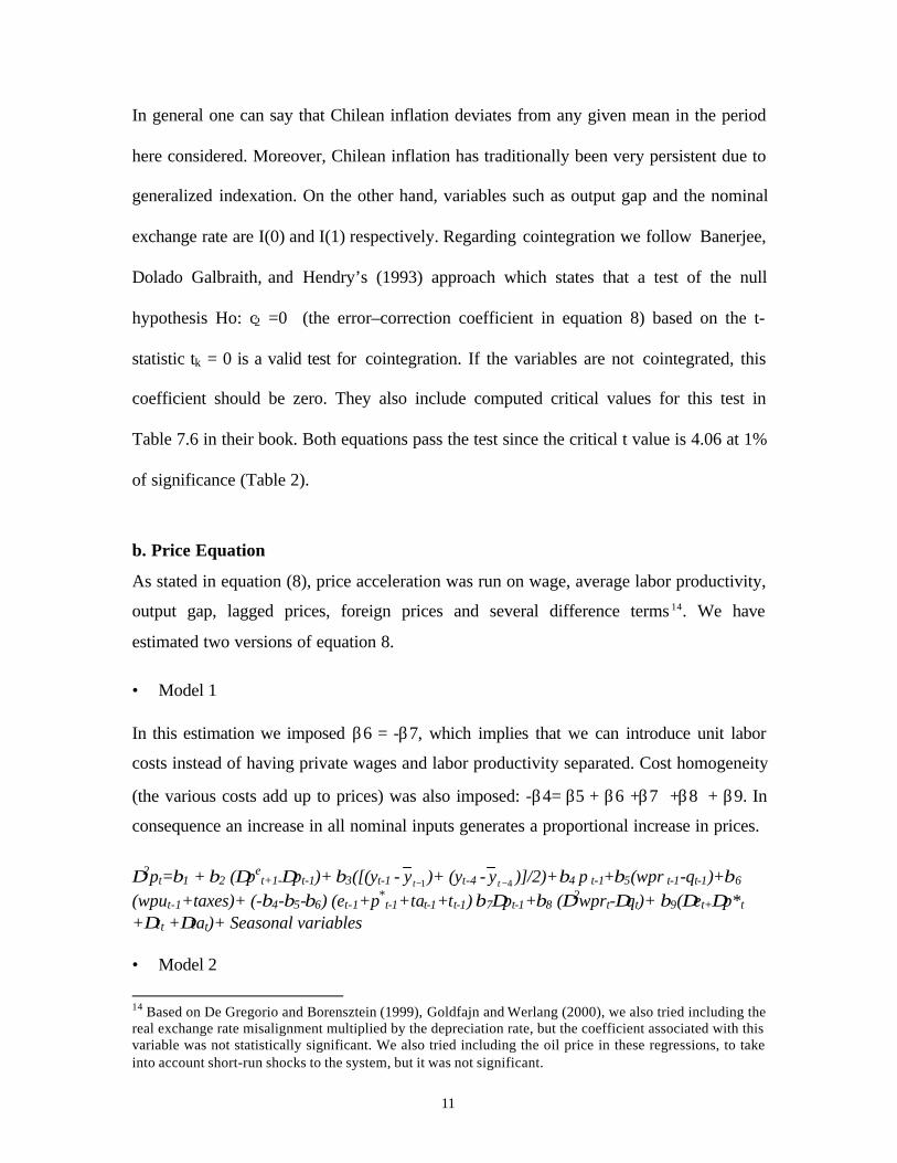
b. Price Equation

As stated in equation (8), price acceleration was run on wage, average labor productivity,

output gap, lagged prices, foreign prices and several difference terms 14. We have

estimated two versions of equation 8.

• Model 1

In this estimation we imposed β6 = -β7, which implies that we can introduce unit labor

costs instead of having private wages and labor productivity separated. Cost homogeneity

(the various costs add up to prices) was also imposed: -β4= β5 + β6 +β7 +β8 + β9. In

consequence an increase in all nominal inputs generates a proportional increase in prices.

∆2pt=β1 + β2 (∆pet+1-∆pt-1)+ β3([(yt-1 - 1−ty )+ (yt-4 - 4−ty )]/2)+β4 p t-1+β5(wpr t-1-qt-1)+β6

(wput-1+taxes)+ (-β4-β5-β6) (et-1+p*t-1+tat-1+tt-1) β7∆pt-1+β8 (∆2wprt-∆qt)+ β9(∆et+∆p*t

+∆tt +∆tat)+ Seasonal variables

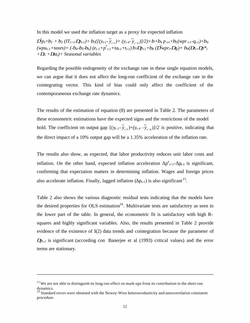
• Model 2

14 Based on De Gregorio and Borensztein (1999), Goldfajn and Werlang (2000), we also tried including thereal exchange rate misalignment multiplied by the depreciation rate, but the coefficient associated with thisvariable was not statistically significant. We also tried including the oil price in these regressions, to takeinto account short-run shocks to the system, but it was not significant.

12

In this model we used the inflation target as a proxy for expected inflation

∆2pt=β1 + β2 (ITt+1-∆pt-1)+ β3([(yt-1- 1−ty )+ (yt-4- 4−ty )]/2)+β+β4 p t-1+β5(wpr t-1-qt-1)+β6

(wput-1+taxes)+ (-β4-β5-β6) (et-1+p*t-1+tat-1+tt-1) β7∆pt-1+β8 (∆2wprt-∆qt)+ β9(∆et+∆p*t

+∆tt +∆tat)+ Seasonal variables

Regarding the possible endogeneity of the exchange rate in these single equation models,

we can argue that it does not affect the long-run coefficient of the exchange rate in the

cointegrating vector. This kind of bias could only affect the coefficient of the

contemporaneous exchange rate dynamics.

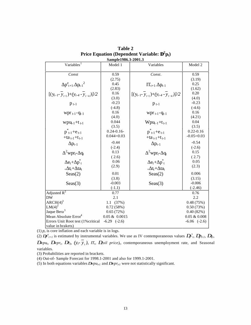
The results of the estimation of equation (8) are presented in Table 2. The parameters of

these econometric estimations have the expected signs and the restrictions of the model

hold. The coefficient on output gap [(yt-1- 1−ty )+(yt-4 - 4−ty )]/2 is positive, indicating that

the direct impact of a 10% output gap will be a 1.35% acceleration of the inflation rate.

The results also show, as expected, that labor productivity reduces unit labor costs and

inflation. On the other hand, expected inflation acceleration ∆pet+1-∆pt-1 is significant,

confirming that expectation matters in determining inflation. Wages and foreign prices

also accelerate inflation. Finally, lagged inflation (∆pt-1) is also significant15.

Table 2 also shows the various diagnostic residual tests indicating that the models have

the desired properties for OLS estimation16. Multivariate tests are satisfactory as seen in

the lower part of the table. In general, the econometric fit is satisfactory with high R-

squares and highly significant variables. Also, the results presented in Table 2 provide

evidence of the existence of I(2) data trends and cointegration because the parameter of

∆pt-1 is significant (according con Banerjee et al (1993) critical values) and the error

terms are stationary.

15 We are not able to distinguish its long-run effect on mark-ups from its contribution to the short-rundynamics.16 Standard errors were obtained with the Newey-West heteroscedasticity and autocorrelation consistentprocedure.

13

Table 2Price Equation (Dependent Variable: ∆∆2pt)

Sample1986.3-2001.3Variables1 Model 1 Variables Model 2

Const 0.59(2.75)

Const. 0.59(3.19)

∆pet+1-∆pt-1

2 0.45(2.83)

ITt+1-∆pt-1 0.25(1.62)

[(yt-1- 1−ty )+(yt-4 - 4−ty )]/2 0.16(3.0)

[(yt-1- 1−ty )+(yt-4 - 4−ty )]/2 0.20(4.0)

p t-1 -0.23(-4.8)

p t-1 -0.23(-4.6)

wpr t-1-qt-1 0.16(4.0)

wpr t-1-qt-1 0.16(4.21)

wput-1+t t-1 0.044(3.5)

Wput-1+t t-1 0.04(3.5)

p*t-1+e t-1

+ta t-1+t t-10.24-0.16-0.044=0.03

p*t-1+e t-1

+ta t-1+t t-10.22-0.16

-0.05=0.03

∆pt-1 -0.44(-2.4)

∆pt-1 -0.54(-2.6)

∆2wprt-∆qt 0.13( 2.6)

∆2wprt-∆qt 0.15( 2.7)

∆et+∆p*t

+∆tt+∆tat

0.06(2.9)

∆et+∆p*t

+∆tt+∆tat

0.05(2.3)

Seas(2) 0.01(3.8)

Seas(2) 0.006(3.15)

Seas(3) -0.003(-1.1)

Seas(3) -0.006(-2.46)

Adjusted R2

DWARCH(4)3

LM(4)3

Jaque Bera3

Mean Absolute Error4

Errors Unit Root test (1%criticalvalue in brakets)

0.772.1

1.1 (37%)0.72 (58%)0.65 (72%)

0.05 & 0.0015 -6.29 (-2.6)

0.762.2

0.48 (75%)0.50 (73%)0.40 (82%)

0.05 & 0.008-6.06 (-2.6)

(1) pt is core inflation and each variable is in logs.(2) ∆pe

t+1 is estimated by instrumental variables. We use as IV contemporaneous values ∆p*t, ∆pt-1, ∆qt,

∆wput, ∆wprt, ∆et, (yt- ty ), ITt, ∆(oil price)t, contemporaneous unemployment rate, and Seasonal

variables.(3) Probabilities are reported in brackets.(4) Out-of- Sample Forecast for 1998.1-2001 and also for 1999.1-2001.(5) In both equations variables ∆wput-1 and ∆wprt-1 were not statistically significant.

14

We tested the two restrictions of model 1 using an unrestricted version of it. First, we

tested the hypothesis of the coefficient on private wages being equal to the one on labor

productivity, though with opposite signs. If this is the case we can include unit labor cost

(w-q) as a variable in the model.

Table 3Restrictions Tests on Model 1

Wald Test Hypothesis Model 1Unit Labor Cost 90%Linear Homogeneity andUnit Labor Cost

61%

As shown in Table 3, the Wald test indicates that we fail to reject the null hypothesis of

different coefficients at 90% of significance. Second, we tested in Model 1 the hypothesis

that the various costs add up to prices (cost homogeneity). We also fail to reject this null

hypothesis at a 61% of significance (Table 3). As a result we imposed both restrictions in

Model 1.

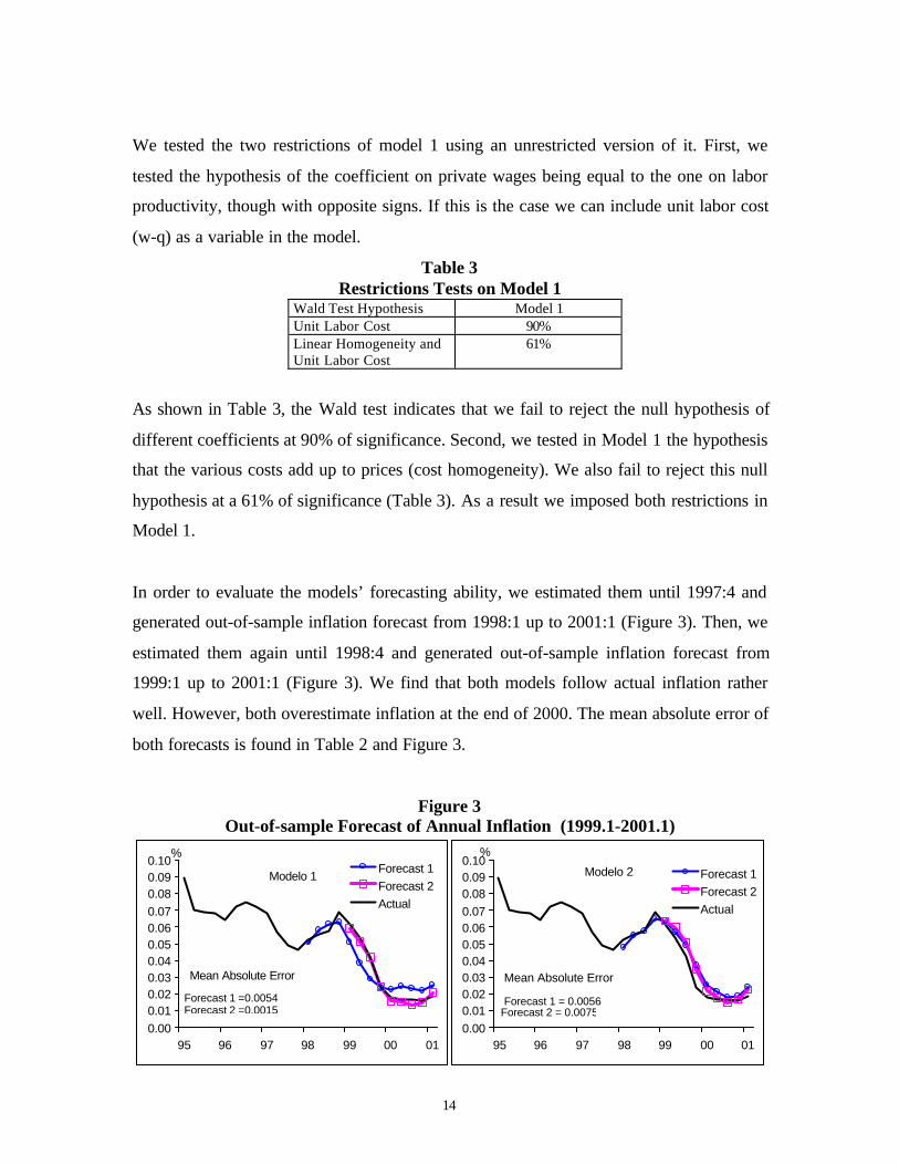
In order to evaluate the models’ forecasting ability, we estimated them until 1997:4 and

generated out-of-sample inflation forecast from 1998:1 up to 2001:1 (Figure 3). Then, we

estimated them again until 1998:4 and generated out-of-sample inflation forecast from

1999:1 up to 2001:1 (Figure 3). We find that both models follow actual inflation rather

well. However, both overestimate inflation at the end of 2000. The mean absolute error of

both forecasts is found in Table 2 and Figure 3.

Figure 3Out-of-sample Forecast of Annual Inflation (1999.1-2001.1)

0.000.010.020.030.040.050.060.070.080.090.10

95 96 97 98 99 00 01

Forecast 1Forecast 2Actual

%

Modelo 1

Mean Absolute Error

Forecast 1 =0.0054Forecast 2 =0.0015

0.000.010.020.030.040.050.060.070.080.090.10

95 96 97 98 99 00 01

Forecast 1Forecast 2Actual

%Modelo 2

Mean Absolute Error

Forecast 1 = 0.0056Forecast 2 = 0.0075

15

c. Pass-Through17

Finally, we analyze the implications of our estimations on exchange rate pass-through by

simulating an unexpected permanent 10% shock to the nominal exchange rate18. In order

to do so, besides using the estimated equation (first column in Table 2), we assume fully

indexed wages. Thus, we solve the model (not estimate it) simultaneously, by also

including the following equation: wt = wt-1 + ∆pt-1, for both private and public sectors,

respectively. After we introduce a shock to the nominal exchange rate, we compute the

pass-through effect using the simulated paths followed by both the nominal exchange rate

and domestic prices. It is worth noting that the exercise does not consider any monetary

policy action.

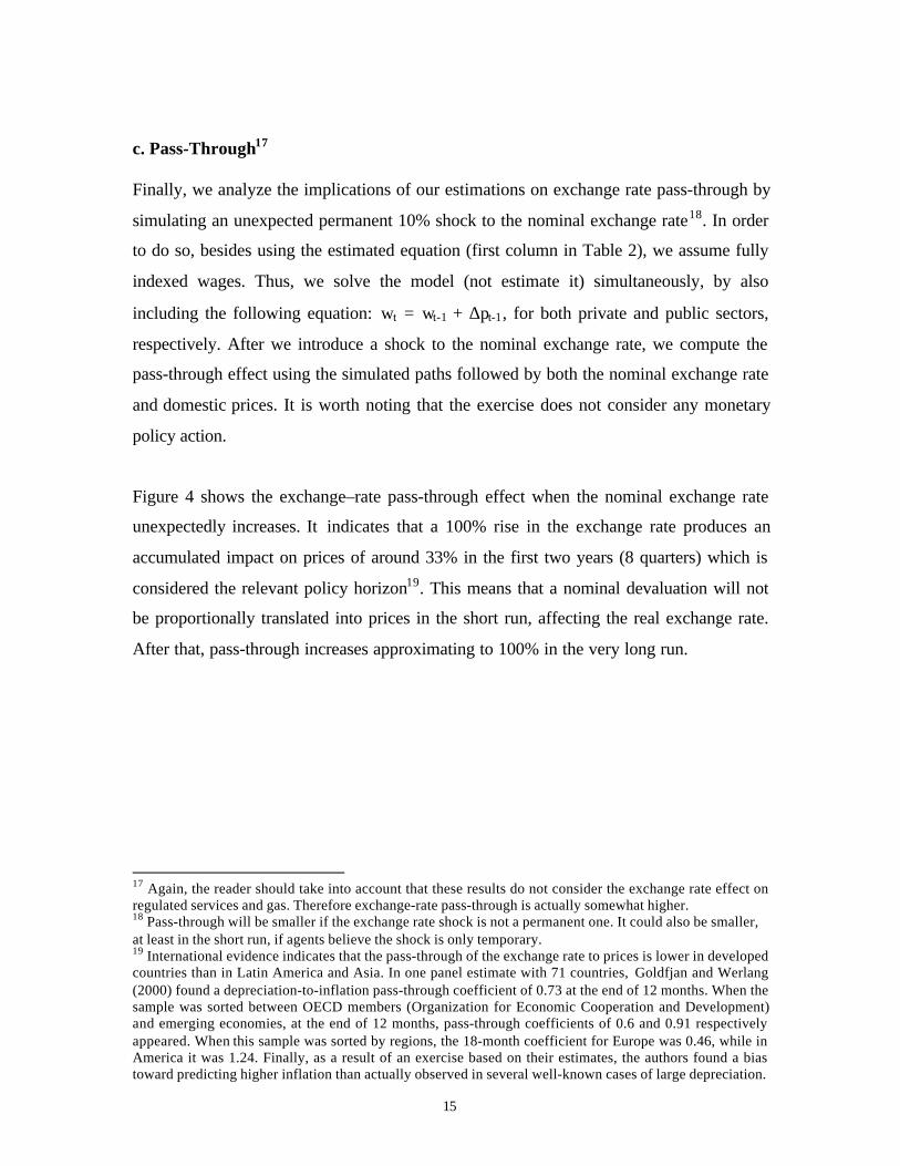
Figure 4 shows the exchange–rate pass-through effect when the nominal exchange rate

unexpectedly increases. It indicates that a 100% rise in the exchange rate produces an

accumulated impact on prices of around 33% in the first two years (8 quarters) which is

considered the relevant policy horizon19. This means that a nominal devaluation will not

be proportionally translated into prices in the short run, affecting the real exchange rate.

After that, pass-through increases approximating to 100% in the very long run.

17 Again, the reader should take into account that these results do not consider the exchange rate effect onregulated services and gas. Therefore exchange-rate pass-through is actually somewhat higher.18 Pass-through will be smaller if the exchange rate shock is not a permanent one. It could also be smaller,at least in the short run, if agents believe the shock is only temporary.19 International evidence indicates that the pass-through of the exchange rate to prices is lower in developedcountries than in Latin America and Asia. In one panel estimate with 71 countries, Goldfjan and Werlang(2000) found a depreciation-to-inflation pass-through coefficient of 0.73 at the end of 12 months. When thesample was sorted between OECD members (Organization for Economic Cooperation and Development)and emerging economies, at the end of 12 months, pass-through coefficients of 0.6 and 0.91 respectivelyappeared. When this sample was sorted by regions, the 18-month coefficient for Europe was 0.46, while inAmerica it was 1.24. Finally, as a result of an exercise based on their estimates, the authors found a biastoward predicting higher inflation than actually observed in several well-known cases of large depreciation.

16

Figure 4Exchange Rate Pass-Through Simulation

0.00

0.02

0.04

0.06

0.08

0.10

0.12

1 5 9 13 17 21 25 29 33 37 41 45

Prices with Output Gap

Prices

Prices with Incomplete Wage

Indexation

Nominal Exchange Rate

00.10.20.30.40.50.60.70.80.9

1

1 5 9 13 17 21 25 29 33 37 41 45

Pass-Through

Pass-Through Incomplete Wage

Indexation

Pass-Through with Output Gap

We also realized an exercise imposing the limitation that private wages do not have full

indexation: wt = wt-1 + 0.9*∆pt-1. Figure 4 shows that in this case, pass-through is much

smaller in the long run. Nonetheless, this effect is not large in the first two years. Of

course, this scenario assumes that private wages will permanently bear the cost of a

higher nominal exchange rate, which is not realistic.

Evidence suggests that there is a pass-through decrease when the output is below

potential (recession) because a negative output gap tends to compensate the inflationary

effect of depreciation by reducing margins. This is what usually happens when a currency

depreciation is the result of a negative terms of trade shock with negative effects on

output (Mishkin, 2001). Figure 4 shows that the exchange-rate effect is much smaller

when there is an exogenous 2% negative output gap, which fades linearly in 3 years. In

this case, a 100% increase in the exchange rate will translate into a 13,5% price increase

i.e. less than half of what it was before. Hence, a fraction of the depreciation is not passed

on to consumers. In the long run, as output gap disappears, pass-through approaches

100%20.

IV. Conclusions

A price equation based on a model of imperfect competition was estimated and used to

generate out-of-sample forecasts for core inflation. The parameters of these econometric

estimations have the expected signs and the restrictions of the model hold. It was

20 Since 1998 the output gap in Chile has probably been higher than what we assumed for this simulation.

17

empirically found, as expected, that labor productivity reduces unit labor costs and

inflation. On the other hand, expected inflation acceleration ∆pet+1-∆pt-1 is significant,

confirming that expectation matters for determining inflation. Wages and foreign prices

are also positively related to inflation. The coefficient on output gap (yt-1- 1−ty ) is positive,

indicating that the direct impact of a 10% output gap will be a 1.6% acceleration of the

inflation rate.

We analyze the implications of our estimations on exchange rate pass-through by

simulating an unexpected permanent 10% shock to the nominal exchange rate. A nominal

devaluation has real effects that disappear in the long run. In the case of incomplete wage

indexation, pass-through is much smaller in the long run. Nonetheless, this effect is not

large in the first two years.

The simulation also shows that a negative output gap tends to compensate the inflationary

effect of depreciation since exchange–rate pass-through depends positively on economic

activity. In this case, a fraction of the depreciation is not passed on to prices in the short

run, explaining why pass-through has been so low in recent years. However, as time goes

on and the output gap disappears, pass-through approaches 100%.

If the recent peso depreciation in Chile is permanent, one can conclude from the results,

that pass-through will increase as soon as aggregate demand starts recuperating.

Nevertheless, this will only be the case if monetary authorities take no action.

18

VII. Bibliography

Banerjee, A., L. Cockerell and B. Russell (2001). “An I(2) Analysis of Inflation and theMarkup.” Journal of Applied Econometrics 16 (3): 221-240.

Banerjee, A., J. Dolado, J. Galbraith and D. Hendry (1993). Co-Integration, Error–Correction, and the Econometric Analysis of Non-Stationary Data. Oxford UniversityPress.

Beaumont, C. V. Cassino and D. Mayes (1994). "Approaches to Modelling Prices at theReserve Bank of New Zealand," Reserve Bank of New Zealand Discussion Paper No.3.

Benabou, R. (1992). “Inflation and Markups: Theories and Evidence from the RetailTrade Sector.” European Economic Review 36: 566-574.

De Gregrorio, J. and E. Borensztein (1999). “Devaluation and Inflation after CurrencyCrises.” Mimeo, IMF Research Department.

Engsted and Haldrup (1999). "Estimating the LQAC Model with I(2) variables." Journalof Applied Econometrics 14: 155-170.

García, P., L. Herrera, and R. Valdés (2000). “New Frontiers for Monetary Policy inChile.” Mimeo, Central Bank of Chile.

Goldberg, P., and M. Knetter (1997). “Goods Prices and Exchange Rates: What Have WeLearned?” Journal of Economic Literature 35 (3), September.

Goldfajn, I., and S. Werlang (2000). “The Pass-through from Depreciation to Inflation: APanel Study.” Working Paper of the Central Bank of Brazil, July.

Haldrup N. (1994). "The Asymptotics of Single-Equation Cointegration Regressions withI(1) and I(2) Variables." Journal of Econometrics 63: 153-181.

Haldrup N. (1995). "An Econometric Analysis of I(2) Variables." Journal of EconomicSurveys 12 (5).

Harris R. (1995). Using Cointegration Analysis in Econometric Modelling. Chapter 4,Prentice Hall.

Haskel, J. C., M. and I. Small (1995). "Price, Marginal cost and the Business Cycle."Oxford Bulletin of Economics and Statistics 57 (1).

Inder, B. (1993). "Estimating Long-run Relationships in Economics: a Comparison ofDifferent Approaches." Journal of Econometrics 57: 53-68.

Johansen, S. (1992). “Testing Weak Exogeneity and the Order of Cointegration in UKMoney Demand Data.” Journal of Policy Modelling 14: 313-34.

19

Kim, K. (1998). US Inflation and the Dollar Exchange Rate a Vector Error CorrectionModel." Applied Economics 30: 613-619.

Kim, Y. (1990). "Exchange Rates and Import Prices in the United States: A Varying-Parameter Estimation of Exchange-Rate Pass-Through." Journal of Business & EconomicStatistics 8(3), July.

Kreps, D. and J. Scheinkman (1983). “Quantity Pre-Commitment and BertrandCompetition Yield Cournot Outcomes.” Rand Journal of Economics 14: 326-337.

Layard, R, S. Nickell and R. Jackman (1991). Unemployment. MacroeconomicPerformance and the labor market. Oxford University Press. Spanish version translatedand Edited by the Ministry of Labor and Social Security of Spain.

McCarthy J. (1999). "Pass-Through of Exchange Rates and Import Prices to DomesticInflation in Some Industrialised Economies." BIS Working Paper No. 79, November.

McCallum, B. (1976). "Rational Expectations and the Natural Rate Hypothesis: SomeConsistent Estimates." Econometrica 44: 43-52.

Mishkin, F. (2001). "The Transmission Mechanism and the Role of Asset Prices inMonetary Policy." National Bureau of Economic Research, Working Paper No. 8617.

Orphanides, A. and V. Wieland (2000). “Inflation Zone Targeting.” European EconomicReview 44(7):1351-1388.

Phillips, P. (1986). "Understanding Spurious regressions in econometrics.” Journal ofEconometrics 33: 335-346.

Phillips P. And M. Loretan (1991). “Estimating Long-run Economic Equilibria.” Reviewof Economic Studies 58: 407-436.

Roberts, J. (1995). “New Keynesian Economics and the Phillips Curve.” Journal ofMoney, Credit, and Banking 27 (4), November.

Roberts, J. (2001). “How Well Does the New Keynesian Sticky-Price Model Fit theData?” Finance and Economic Discussion Papers No. 13, Board of Governors of theFederal Reserve System, February.

Rotemberg, J. (1982). “Sticky Prices in the United States.” Journal of Political Economy60, November.

Rotemberg, J. and G. Saloner (1986). “A Supergame Theoretic Model of Price WarsDuring Booms.” American Economic Review 76: 390-407.

Rotemberg, J. and M. Woodford (1991). “Mark-ups and the Business Cycle.” NBERMacroeconomics Annual, 6.

20

Russel, B., Evans, J. and B. Preston (1997). “The impact of Inflation and Uncertainty onthe Optimum Price Set by Firms.” Department of Economic Studies Discussion Papers,No. 84, University of Dundee.

Small, I. (1997). “The Cyclicality of Mark-ups and Profit Margins: Some Evidence forManufacturing Services.” Working Paper of the Bank of England.

Taylor, J. (2000). "Low Inflation, Pass-Through, and the Pricing Power of Firms."European Economic Review 44(7):1389-408.

Woo W. (1984). "Exchange Rates and the Prices of Nonfood, Non-fuel Products."Brookings Papers on Economic Activity 2.

Documentos de TrabajoBanco Central de Chile

Working PapersCentral Bank of Chile

NÚMEROS ANTERIORES PAST ISSUES

La serie de Documentos de Trabajo en versión PDF puede obtenerse gratis en la dirección electrónica:http://www.bcentral.cl/Estudios/DTBC/doctrab.htm. Existe la posibilidad de solicitar una copiaimpresa con un costo de $500 si es dentro de Chile y US$12 si es para fuera de Chile. Las solicitudes sepueden hacer por fax: (56-2) 6702231 o a través de correo electrónico: bcch@condor.bcentral.cl

Working Papers in PDF format can be downloaded free of charge from:http://www.bcentral.cl/Estudios/DTBC/doctrab.htm. Printed versions can be ordered individually forUS$12 per copy (for orders inside Chile the charge is Ch$500.) Orders can be placed by fax: (56-2) 6702231or e-mail: bcch@condor.bcentral.cl

DTBC-127A Critical View of Inflation Targeting: Crises, LimitedSustainability, and Agregate ShocksMichael Kumhof

Noviembre 2001

DTBC-126Overshootings and Reversals: The Role of Monetary PolicyIlan Goldfajn y Poonam Gupta

Noviembre 2001

DTBC-125New Frontiers for Monetary Policy in ChilePablo S. García, Luis Oscar Herrera y Rodrigo O. Valdés

Noviembre 2001

DTBC-124Monetary Policy under Flexible Exchange Rates: An Introduction toInflation TargetingPierre-Richard Agénor

Noviembre 2001

DTBC-123Targeting Inflation in an Economy with Staggered Price SettingJordi Galí

Noviembre 2001

DTBC-122Market Discipline and Exuberant Foreign BorrowingEduardo Fernández-Arias y Davide Lombardo

Noviembre 2001

DTBC-121Japanese Banking Problems: Implications for Southeast AsiaJoe Peek y Eric S. Rosengren

Noviembre 2001

DTBC-120The 1997-98 Liquidity Crisis: Asia versus Latin AmericaRoberto Chang y Andrés Velasco

Noviembre 2001

DTBC-119Politics and the Determinants of Banking Crises: The effects ofPolitical Checks and BalancesPhilip Keefer

Noviembre 2001

DTBC-118Financial Regulation and Performance: Cross-Country EvidenceJames R. Barth, Gerard Caprio, Jr. y Ross Levine

Noviembre 2001

DTBC-117Some Measures of Financial Fragility in the Chilean BankingSystem: An Early Warning Indicators ApplicationAntonio Ahumada C. y Carlos Budnevich L.

Noviembre 2001

DTBC-116Inflation Targeting in the Context of IMF-Supported AdjustmentProgramsMario I. Blejer, Alfredo M. Leone, Pau Rabanal y Gerd Schwartz

Noviembre 2001

DTBC-115A Decade of Inflation Targeting in Chile: Developments, Lessons,and ChallengesFelipe Morandé

Noviembre 2001

DTBC-114Inflation Targets in a Global ContextGabriel Sterne

Noviembre 2001

DTBC-113Lessons from Inflation Targeting in New ZealandAaron Drew

Noviembre 2001

DTBC-112Inflation Targeting and the Liquidity TrapBennett T. McCallum

Noviembre 2001

DTBC-111Inflation Targeting and the Inflation Process: Lessons from anOpen EconomyGuy Debelle y Jenny Wilkinson

Noviembre 2001