Bakshi, Kapadia, and Madan (2003) Risk-Neutral Moment Estimators · 2019-11-28 ·...
49
Bakshi, Kapadia, and Madan (2003) Risk-Neutral Moment Estimators * Pakorn Aschakulporn † Department of Accountancy and Finance Otago Business School, University of Otago Dunedin 9054, New Zealand [email protected] Jin E. Zhang Department of Accountancy and Finance Otago Business School, University of Otago Dunedin 9054, New Zealand [email protected] First Version: 11 April 2019 This Version: 14 November 2019 Keywords: Risk-neutral moment estimators JEL Classification Code: G13 * Jin E. Zhang has been supported by an establishment grant from the University of Otago and the National Natural Science Foundation of China grant (Project No. 71771199). † Corresponding author. Tel: +64 21 039 8000.
Transcript of Bakshi, Kapadia, and Madan (2003) Risk-Neutral Moment Estimators · 2019-11-28 ·...

Bakshi, Kapadia, and Madan (2003) Risk-NeutralMoment Estimators∗
Pakorn Aschakulporn†
Department of Accountancy and FinanceOtago Business School, University of Otago
Dunedin 9054, New [email protected]
Jin E. ZhangDepartment of Accountancy and Finance
Otago Business School, University of OtagoDunedin 9054, New Zealand
First Version: 11 April 2019This Version: 14 November 2019
Keywords: Risk-neutral moment estimatorsJEL Classification Code: G13
∗ Jin E. Zhang has been supported by an establishment grant from the University of Otago and theNational Natural Science Foundation of China grant (Project No. 71771199).† Corresponding author. Tel: +64 21 039 8000.
i
Bakshi, Kapadia, and Madan (2003) Risk-NeutralMoment Estimators
Abstract
This is the first study of the errors of the Bakshi, Kapadia, and Madan (2003) risk-neutral moment estimators with the density of the underlying explicitly specified. Thiswas accomplished using the Gram-Charlier expansion. To obtain skewness with (absolute)errors less than 10−3, the range of strikes (Kmin, Kmax) must contain at least 3/4 to 4/3 ofthe forward price and have a step size (∆K) of no more than 0.1% of the forward price.The range of strikes and step size corresponds to truncation and discretisation errors,respectively.
Keywords: Risk-neutral moment estimatorsJEL Classification Code: G13
Bakshi, Kapadia, and Madan (2003) Risk-Neutral Moment Estimators 1
1 Introduction
Risk-neutral moment estimators are functions which convert option prices to the moments
of the underlying asset. These estimators are much more complicated than the estima-
tors for physical moments, as physical moments can be obtained from an underlying
asset’s return using standard statistical methods. The moments most used are the first
and second moments, which correspond to the mean and variance, respectively. Higher
(standardised) moments include the third and fourth moments which correspond to the
skewness and kurtosis, respectively. These moments can be used to form a basis of un-
derstanding of the behaviour of the asset. For a more practical use, the third risk-neutral
moment for the S&P500 is the basis for the Chicago Board Options Exchange (CBOE)
skewness (SKEW) index. The SKEW1 was designed to capture the tail-risk. The method
used to calculate the risk-neutral moments in the CBOE SKEW is Bakshi, Kapadia, and
Madan (2003), which will now be referred to as BKM. As with all numerical calculations
the BKM calculations too have errors. This paper examines the error and convergence of
BKM’s risk-neutral skewness and kurtosis estimators and finds the region in which the
errors of the skewness estimator is bounded by 10−3.
The BKM is an extension of Demeterfi, Derman, Kamal, and Zou (1999) and Carr
and Madan (2001b) which propose methods to price variance swaps via static replication
using options. Volatility swaps (viz. realized volatility forward contracts) provide pure
exposure to volatility in contrast to trading volatility through stock options which are im-
pure as it is contaminated by the option’s dependence on the stock price. This underpins
the CBOE VIX, the volatility index of the S&P500. The BKM method now provides the
foundation for recent literature with regard to risk-neutral moment estimators. Neumann
and Skiadopoulos (2013), Conrad, Dittmar, and Ghysels (2013), Chang, Christoffersen,
and Jacobs (2013), and Stilger, Kostakis, and Poon (2017) studied the time-series re-
lationship between BKM risk-neutral moments and the equity market. Cheng (2018)
1 http://www.cboe.com/products/vix-index-volatility/volatility-indicators/skew

Bakshi, Kapadia, and Madan (2003) Risk-Neutral Moment Estimators 2
studied the time-series relationship between BKM risk-neutral moments and the VIX.
Chatrath, Miao, Ramchander, and Wang (2016) and Ruan and Zhang (2018) studied the
time-series relationship between BKM risk-neutral moments and the crude oil market.
Christoffersen, Jacobs, and Chang (2011) summarises various risk-neutral estimators in-
cluding those for volatility, skewness, and kurtosis with respect to their underlying asset
for various markets. Bakshi and Madan (2006) study the spread between risk-neutral and
physical volatilities of the S&P100 index. Liu and Faff (2017) propose a forward-looking
market symmetric index which is used to compete with the CBOE SKEW and therefore
the BKM method.
Liu and van der Heijden (2016) and Lee and Yang (2015) study the errors of the BKM
method when the true value of the risk-neutral moment is unknown. Liu and van der
Heijden (2016) uses various option pricing models to create their benchmark risk-neutral
moments. This was done using Monte Carlo simulations on the Black-Scholes-Merton
model (Black and Scholes, 1973; Merton, 1973), Heston stochastic volatility model (Hes-
ton, 1993), Merton jump-diffusion model (Merton, 1976), and Bates stochastic volatility
jump-diffusion model (combination of Merton and Heston models) (Bates, 1996). As
simulations are used, the benchmark is expected to converge to the true value as more
simulations are made. Lee and Yang (2015) uses historical information to calibrate their
benchmark Black-Scholes model and uses the benchmark to compare with the Bates
stochastic volatility jump-diffusion model. The values of the risk-neutral estimators are
not calculated, instead, the errors are determined relative to the benchmark. The Black-
Scholes model has also been used as a benchmark by Dennis and Mayhew (2002) and
Jiang and Tian (2005). Both Liu and van der Heijden (2016) and Lee and Yang (2015)
study the errors of the BKM method with little control over the inputs. They, therefore,
only have approximations of the true moments and introduces additional errors into their
analysis.
In this paper, the benchmark used is created following Zhang and Xiang (2008) in
Bakshi, Kapadia, and Madan (2003) Risk-Neutral Moment Estimators 3
using the Gram-Charlier series to create virtual options. These options are created by
specifying parameters such as the skewness and excess kurtosis (hereinafter, kurtosis).
The Gram-Charlier series has been used in many papers, for example, Backus, Foresi,
and Wu (2004), Longstaff (1995), and Jarrow and Rudd (1982). Using these options,
the BKM estimators are applied and compared to the true moments used to create the
options. Both the BKM methodology and Gram-Charlier series can be used to calculate
the VIX. In addition to the moments, these two methods are also compared.
The remainder of this paper is organized as follows. Section 2 presents the method
used to create virtual options, a brief dive into how BKM determines the risk-neutral
skewness, and the method used to quantify and analyse the errors and convergence of the
BKM method. Section 3 describes the data. Section 4 provides the numerical results and
Section 6 concludes. The appendix gives the details of key derivations.
2 Methodology
2.1 Creating Virtual Options
To test the BKM higher-order risk-neutral moment estimators, virtual options with known
properties can be created using Zhang and Xiang (2008) as a basis. The options are
created based on the probability density function of the return of the underlying asset.
The density used in basic models tends to be based on the normal distribution function.
However, the returns of stocks are known to have both skewness and kurtosis which are not
modelled by the symmetric normal distribution. The Gram-Charlier series can be used to
create a new density based on the normal distribution function with specified skewness and
kurtosis. This series is similar to the Taylor series; however, it also combines probability
densities by using Hermite polynomials. The Gram-Charlier series used is given by
f(y) = n(y)− λ1
3!d3n(y)dy3 + λ2
4!d4n(y)dy4 , (1)
Bakshi, Kapadia, and Madan (2003) Risk-Neutral Moment Estimators 4
where n(y) = 1√2πe− y
22 , λ1 is the skewness, and λ2 is the kurtosis. The density has a
mean, variance, skew, and kurtosis of 0, 1, λ1, and λ2, respectively.
[Insert Figure 1 about here.]
Figure 1 shows the region of skewness and kurtosis, which ensures a valid density function.
The derivation of this region is shown in appendix A.
The stock price at maturity, ST , can be modelled by
ST = F Tt e
(− 12σ
2+µc)τ+σ√τy, (2)
where F Tt , σ, τ , and µc is the forward price, standard deviation, time to maturity (T − t),
and convexity adjustment term, respectively. The forward price, F Tt , is related to the
current stock price (St) by F Tt = Ste
(r−q)τ , where q is the continuous dividend rate. The
convexity adjustment term, µc, is required to keep this model in the risk-neutral world
(by ensuring that the stock price satisfies the martingale condition). From this, the price
of a European call option will be
ct = e−rτEQt [max(ST −K, 0)] . (3)
In terms of F Tt , K, τ, r, σ, λ1, and λ2, the price is
ct = F Tt e−rτN(d1)−Ke−rτN(d2) +Ke−rτ
(λ1
3!A+ λ2
4!B)σ√τ (4)
where
A = −(d2 − σ
√τ)n(d2)
B = −(1− d2
2 + σ√τd2 − σ2τ
)n(d2)
d2 =ln(F T
t /K) +(−1
2σ2 + µc
)τ
σ√τ
, d1 = d2 + σ√τ
For a given set of parameters (F Tt , r, σ, λ1, and λ2), the prices for each virtual option can
be created for a range of strikes, K, and maturities, τ . The derivation of Equation (4) is

Bakshi, Kapadia, and Madan (2003) Risk-Neutral Moment Estimators 5
shown in appendix B. European put options can be found using the put-call parity
ct − pt = F Tt e−rτ −Ke−rτ . (5)
With these virtual European put and call options, the BKM skewness and kurtosis estima-
tors can be examined and compared against the true skewness (λ1) and true kurtosis (λ2),
respectively.
2.2 Calculating BKM Skew and Kurtosis
The BKM method calculates the risk-neutral (return) skewness (n = 3) and kurtosis
(n = 4) using the basic normalized nth central moments (viz. standardised moments)
equation
nth standardised moment =EQt
[(R (t, τ)− EQt [R (t, τ)]
)n]EQt
[(R (t, τ)− EQt [R (t, τ)]
)2]n
2(6)
where R (t, τ) ≡ ln [ST ]− ln [St], the log returns. However, BKM makes a small approxi-
mation to the mean and sets dividends, q, to zero:
EQt [R (t, τ)] ≈ µ(t, τ) = erτ−1− 12EQt
[R (t, τ)2
]− 1
3!EQt
[R (t, τ)3
]− 1
4!EQt
[R (t, τ)4
](7)
The approximation is due to the exclusion of higher-order terms in the expansion of the
exponential function. This approximation serves in a similar manner to the convexity
adjustment term in the addition of higher-order moments, for the BKM method, this is
in the form of volatility (R (t, τ)2), cubic (R (t, τ)3), and quadratic (R (t, τ)4) payoff con-
tracts. These contracts are not standard; therefore, to calculate their values, the contracts
are decomposed into standard, European options, bonds, and shares. Equation 1 of Carr
and Madan (2001a) shows that any twice-differentiable payoff function with bounded ex-
pectation can be spanned by a continuum of out-of-the-money (OTM) European options,
bonds, and shares. For payoff function H (x) ∈ C 2 and some constant x0, the decomposed

Bakshi, Kapadia, and Madan (2003) Risk-Neutral Moment Estimators 6
payoff function is given by
H (x) = H (x0) +Hx (x0) (x− x0) +∫ x0
0Hxx (K) max (K − x, 0) dK
+∫ ∞x0
Hxx (K) max (x−K, 0) dK(8)
Following BKM in using Equation (8), setting ST = S, the dependent variable, and
setting x0 to St, the following payoff
H(S) =
R (t, τ)2 volatility contract (V )R (t, τ)3 cubic contract (W )R (t, τ)4 quartic contract (X)
(9)
results in H (St) = 0, Hx (St) = 0, and
Hxx (K) = n
K2
[(n− 1)
[ln(K
St
)]n−2−[ln(K
St
)]n−1]. (10)
Finally, the expected value of each contract is given by
EQt[e−rτR (t, τ)n
]=∫ ∞
0
n
K2
[(n− 1)
[ln(K
St
)]n−2−[ln(K
St
)]n−1]Q (K) dK (11)
where n specifies the type of power contract and Q (K) corresponds to the OTM option
with strike K. If there exists both put and call at the at-the-money point, then the
average of the two is taken. n = 2, 3, 4 corresponds to the volatility (V ), cubic (W ), and
quadratic (X) payoff contracts, respectively. With these payoff contracts, the skewness
can be calculated using Equation (6). More details are shown in appendix C.
2.3 Testing for Errors and Convergence
There are many different numerical integration techniques; a commonly used technique
is the trapezium rule (viz. trapezoidal integration). Another is Simpson’s rule. The
trapezium rule essentially adds the area of piecewise-linear lines and Simpson’s rule adds
the area of quadratic curves.
As data from the options market is not continuous, the integral calculation of Equa-
tion (11) must be solved numerically. Using the trapezium rule, the integral can be
Bakshi, Kapadia, and Madan (2003) Risk-Neutral Moment Estimators 7
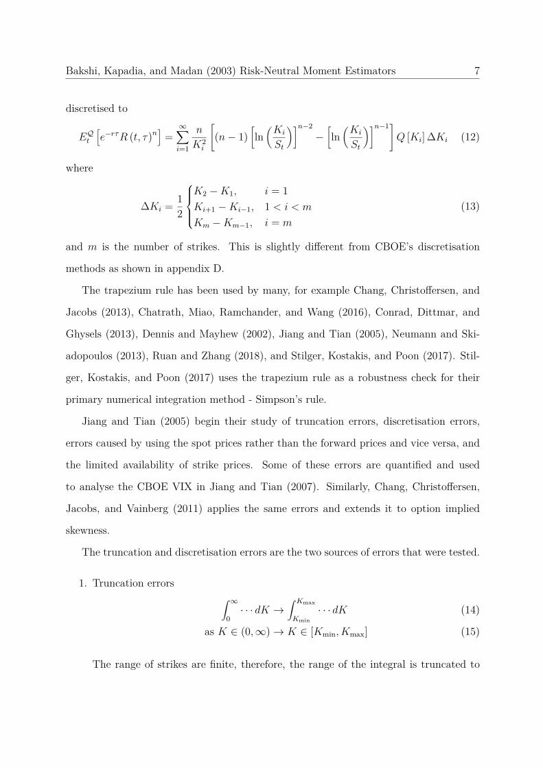
discretised to
EQt[e−rτR (t, τ)n
]=∞∑i=1
n
K2i
[(n− 1)
[ln(Ki
St
)]n−2−[ln(Ki
St
)]n−1]Q [Ki] ∆Ki (12)
where
∆Ki = 12
K2 −K1, i = 1Ki+1 −Ki−1, 1 < i < m
Km −Km−1, i = m
(13)
and m is the number of strikes. This is slightly different from CBOE’s discretisation
methods as shown in appendix D.
The trapezium rule has been used by many, for example Chang, Christoffersen, and
Jacobs (2013), Chatrath, Miao, Ramchander, and Wang (2016), Conrad, Dittmar, and
Ghysels (2013), Dennis and Mayhew (2002), Jiang and Tian (2005), Neumann and Ski-
adopoulos (2013), Ruan and Zhang (2018), and Stilger, Kostakis, and Poon (2017). Stil-
ger, Kostakis, and Poon (2017) uses the trapezium rule as a robustness check for their
primary numerical integration method - Simpson’s rule.
Jiang and Tian (2005) begin their study of truncation errors, discretisation errors,
errors caused by using the spot prices rather than the forward prices and vice versa, and
the limited availability of strike prices. Some of these errors are quantified and used
to analyse the CBOE VIX in Jiang and Tian (2007). Similarly, Chang, Christoffersen,
Jacobs, and Vainberg (2011) applies the same errors and extends it to option implied
skewness.
The truncation and discretisation errors are the two sources of errors that were tested.
1. Truncation errors ∫ ∞0· · · dK →
∫ Kmax
Kmin· · · dK (14)
as K ∈ (0,∞)→ K ∈ [Kmin, Kmax] (15)
The range of strikes are finite, therefore, the range of the integral is truncated to
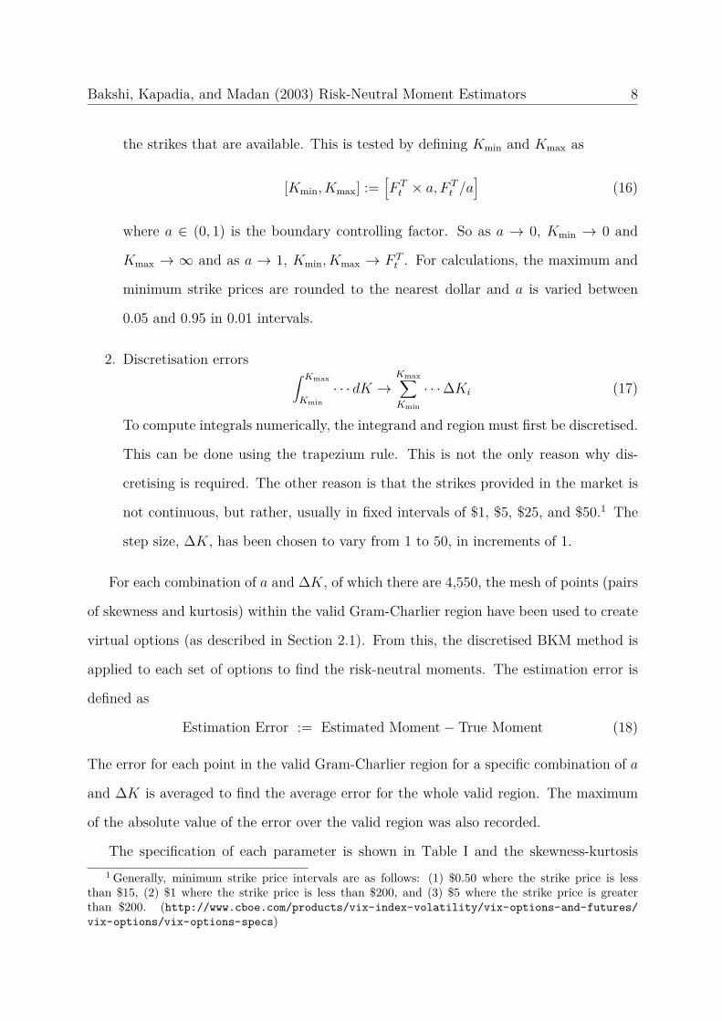
Bakshi, Kapadia, and Madan (2003) Risk-Neutral Moment Estimators 8
the strikes that are available. This is tested by defining Kmin and Kmax as
[Kmin, Kmax] :=[F Tt × a, F T
t /a]
(16)
where a ∈ (0, 1) is the boundary controlling factor. So as a → 0, Kmin → 0 and
Kmax → ∞ and as a → 1, Kmin, Kmax → F Tt . For calculations, the maximum and
minimum strike prices are rounded to the nearest dollar and a is varied between
0.05 and 0.95 in 0.01 intervals.
2. Discretisation errors ∫ Kmax
Kmin· · · dK →
Kmax∑Kmin
· · ·∆Ki (17)
To compute integrals numerically, the integrand and region must first be discretised.
This can be done using the trapezium rule. This is not the only reason why dis-
cretising is required. The other reason is that the strikes provided in the market is
not continuous, but rather, usually in fixed intervals of $1, $5, $25, and $50.1 The
step size, ∆K, has been chosen to vary from 1 to 50, in increments of 1.
For each combination of a and ∆K, of which there are 4,550, the mesh of points (pairs
of skewness and kurtosis) within the valid Gram-Charlier region have been used to create
virtual options (as described in Section 2.1). From this, the discretised BKM method is
applied to each set of options to find the risk-neutral moments. The estimation error is
defined as
Estimation Error := Estimated Moment− True Moment (18)
The error for each point in the valid Gram-Charlier region for a specific combination of a
and ∆K is averaged to find the average error for the whole valid region. The maximum
of the absolute value of the error over the valid region was also recorded.
The specification of each parameter is shown in Table I and the skewness-kurtosis1 Generally, minimum strike price intervals are as follows: (1) $0.50 where the strike price is less
than $15, (2) $1 where the strike price is less than $200, and (3) $5 where the strike price is greaterthan $200. (http://www.cboe.com/products/vix-index-volatility/vix-options-and-futures/vix-options/vix-options-specs)
Bakshi, Kapadia, and Madan (2003) Risk-Neutral Moment Estimators 9
points used in the valid Gram-Charlier region are shown in Figure 2.
[Insert Table I and Figure 2 about here.]
An example of the error calculation for skewness and kurtosis done for the points from
Figure 2 are shown in Figure 3. From this, both the average of the errors and the maximum
absolute error for each region are plotted at their respective boundary controlling factor
and step size.
[Insert Figure 3 about here.]
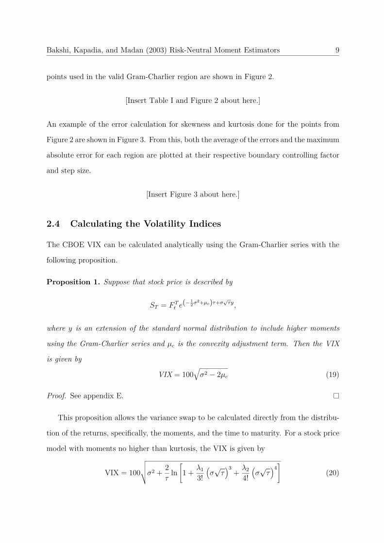
2.4 Calculating the Volatility Indices
The CBOE VIX can be calculated analytically using the Gram-Charlier series with the
following proposition.
Proposition 1. Suppose that stock price is described by
ST = F Tt e
(− 12σ
2+µc)τ+σ√τy,
where y is an extension of the standard normal distribution to include higher moments
using the Gram-Charlier series and µc is the convexity adjustment term. Then the VIX
is given by
VIX = 100√σ2 − 2µc (19)
Proof. See appendix E.
This proposition allows the variance swap to be calculated directly from the distribu-
tion of the returns, specifically, the moments, and the time to maturity. For a stock price
model with moments no higher than kurtosis, the VIX is given by
VIX = 100
√√√√σ2 + 2τ
ln[1 + λ1
3!(σ√τ)3
+ λ2
4!(σ√τ)4]
(20)
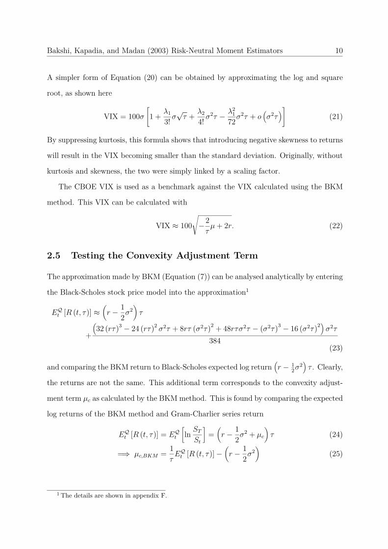
Bakshi, Kapadia, and Madan (2003) Risk-Neutral Moment Estimators 10
A simpler form of Equation (20) can be obtained by approximating the log and square
root, as shown here
VIX = 100σ[1 + λ1
3! σ√τ + λ2
4! σ2τ − λ2
172σ
2τ + o(σ2τ
)](21)
By suppressing kurtosis, this formula shows that introducing negative skewness to returns
will result in the VIX becoming smaller than the standard deviation. Originally, without
kurtosis and skewness, the two were simply linked by a scaling factor.
The CBOE VIX is used as a benchmark against the VIX calculated using the BKM
method. This VIX can be calculated with
VIX ≈ 100√−2τµ+ 2r. (22)
2.5 Testing the Convexity Adjustment Term
The approximation made by BKM (Equation (7)) can be analysed analytically by entering
the Black-Scholes stock price model into the approximation1
EQt [R (t, τ)] ≈(r − 1
2σ2)τ
+
(32 (rτ)3 − 24 (rτ)2 σ2τ + 8rτ (σ2τ)2 + 48rτσ2τ − (σ2τ)3 − 16 (σ2τ)2)
σ2τ
384(23)
and comparing the BKM return to Black-Scholes expected log return(r − 1
2σ2)τ . Clearly,
the returns are not the same. This additional term corresponds to the convexity adjust-
ment term µc as calculated by the BKM method. This is found by comparing the expected
log returns of the BKM method and Gram-Charlier series return
EQt [R (t, τ)] = EQt
[ln STSt
]=(r − 1
2σ2 + µc
)τ (24)
=⇒ µc,BKM = 1τEQt [R (t, τ)]−
(r − 1
2σ2)
(25)
1 The details are shown in appendix F.
Bakshi, Kapadia, and Madan (2003) Risk-Neutral Moment Estimators 11
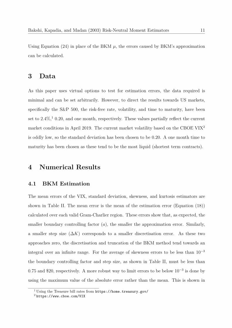
Using Equation (24) in place of the BKM µ, the errors caused by BKM’s approximation
can be calculated.
3 Data
As this paper uses virtual options to test for estimation errors, the data required is
minimal and can be set arbitrarily. However, to direct the results towards US markets,
specifically the S&P 500, the risk-free rate, volatility, and time to maturity, have been
set to 2.4%,1 0.20, and one month, respectively. These values partially reflect the current
market conditions in April 2019. The current market volatility based on the CBOE VIX2
is oddly low, so the standard deviation has been chosen to be 0.20. A one month time to
maturity has been chosen as these tend to be the most liquid (shortest term contracts).
4 Numerical Results
4.1 BKM Estimation
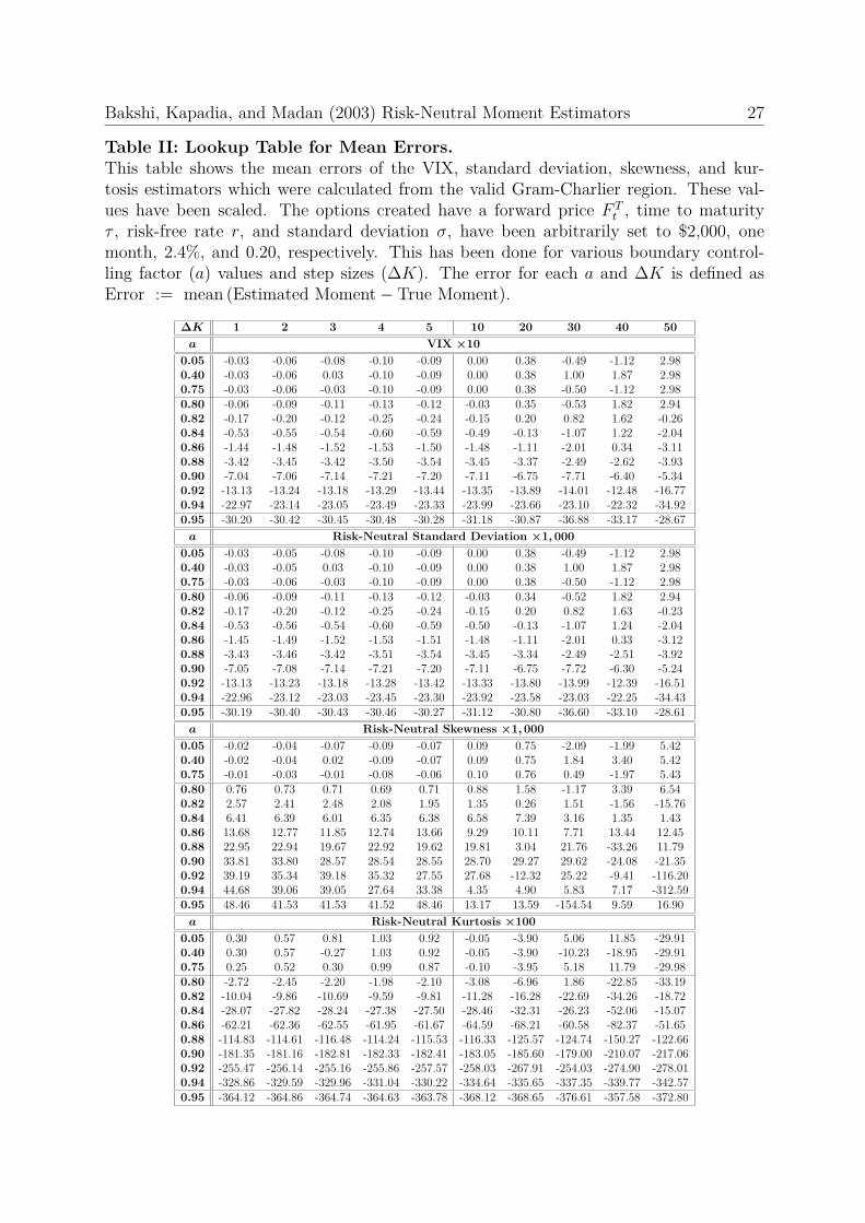
The mean errors of the VIX, standard deviation, skewness, and kurtosis estimators are
shown in Table II. The mean error is the mean of the estimation error (Equation (18))
calculated over each valid Gram-Charlier region. These errors show that, as expected, the
smaller boundary controlling factor (a), the smaller the approximation error. Similarly,
a smaller step size (∆K) corresponds to a smaller discretisation error. As these two
approaches zero, the discretisation and truncation of the BKM method tend towards an
integral over an infinite range. For the average of skewness errors to be less than 10−3
the boundary controlling factor and step size, as shown in Table II, must be less than
0.75 and $20, respectively. A more robust way to limit errors to be below 10−3 is done by
using the maximum value of the absolute error rather than the mean. This is shown in
1 Using the Treasure bill rates from https://home.treasury.gov/2 https://www.cboe.com/VIX
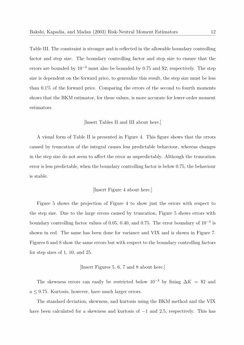
Bakshi, Kapadia, and Madan (2003) Risk-Neutral Moment Estimators 12
Table III. The constraint is stronger and is reflected in the allowable boundary controlling
factor and step size. The boundary controlling factor and step size to ensure that the
errors are bounded by 10−3 must also be bounded by 0.75 and $2, respectively. The step
size is dependent on the forward price, to generalize this result, the step size must be less
than 0.1% of the forward price. Comparing the errors of the second to fourth moments
shows that the BKM estimator, for these values, is more accurate for lower-order moment
estimators.
[Insert Tables II and III about here.]
A visual form of Table II is presented in Figure 4. This figure shows that the errors
caused by truncation of the integral causes less predictable behaviour, whereas changes
in the step size do not seem to affect the error as unpredictably. Although the truncation
error is less predictable, when the boundary controlling factor is below 0.75, the behaviour
is stable.
[Insert Figure 4 about here.]
Figure 5 shows the projection of Figure 4 to show just the errors with respect to
the step size. Due to the large errors caused by truncation, Figure 5 shows errors with
boundary controlling factor values of 0.05, 0.40, and 0.75. The error boundary of 10−3 is
shown in red. The same has been done for variance and VIX and is shown in Figure 7.
Figures 6 and 8 show the same errors but with respect to the boundary controlling factors
for step sizes of 1, 10, and 25.
[Insert Figures 5, 6, 7 and 8 about here.]
The skewness errors can easily be restricted below 10−3 by fixing ∆K = $2 and
a ≤ 0.75. Kurtosis, however, have much larger errors.
The standard deviation, skewness, and kurtosis using the BKM method and the VIX
have been calculated for a skewness and kurtosis of −1 and 2.5, respectively. This has
Bakshi, Kapadia, and Madan (2003) Risk-Neutral Moment Estimators 13
been done for a boundary controlling factor value of 0.05, 0.40, and 0.75 and step size of
1 to 50. This is shown in Figure 9. Figure 10 shows the same errors with respect to the
boundary controlling factors.
[Insert Figures 9 and 10 about here.]
To examine the independence of the skewness estimator from kurtosis, the skewness
is estimated when the skewness, the boundary controlling factor and step size are set to
-1, 0.25 and 1, respectively, whilst adjusting the kurtosis within the valid Gram-Charlier
region. The same has been done for kurtosis when it is set to 2.5. As neither the
true skewness nor the true kurtosis has been chosen to be zero, the relative error for
each estimator can, therefore, be calculated. The (absolute) relative error is defined as
Relative Error =∣∣∣x−xtruextrue
∣∣∣, where x is the estimated value, and xtrue is the true value. The
maximum(minimum) relative error for skewness and kurtosis were found to be 4.476 ×
10−04(4.476× 10−04) and 1.272× 10−03(1.245× 10−03), respectively. These relative error
curves are monotonically increasing and decreasing, as shown in Figure 11. These values
cannot be used to compare the sensitivity of skewness and kurtosis directly. The difference
of the maximum and minimum values for skewness and kurtosis are 5.866 × 10−08 and
2.663×10−05, respectively. From this, the effects of kurtosis on the estimation of skewness
and vice versa are shown to be insignificant. Therefore, for this case, the estimation of
skewness is independent of kurtosis and vice versa.
[Insert Figure 11 about here.]
4.2 In-Depth Error Analysis
A closer inspection of errors shows that the current level of granularity of the step size
∆K = 1 is not sufficient to show the overall form of the relationship between the errors
and step size. By reducing the step size to ∆K = 0.001, this reveals a form which is closer
to the true form. This is shown in Figure 12.

Bakshi, Kapadia, and Madan (2003) Risk-Neutral Moment Estimators 14
[Insert Figure 12 about here.]
The error does not decrease exponentially with respect to the step size, but more
so quadratically. The error envelope, positive (+) and negative (−), was found using a
least-squares approximation of a relatively simple parsimonious quadratic curve
β1∆K + β2(∆K)2. (26)
The coefficients β+1 , β+
2 , β−1 , and β−2 were found to be 2.984 × 10−04, 1.969 × 10−05,
−1.639 × 10−04, and −8.959 × 10−06, respectively. Using these values, the asymmetric
envelope can be decomposed into two components, a symmetric envelope, and a trend
term. The symmetric envelope has parameters βs1 and βs2 equal to 2.311 × 10−04 and
1.433 × 10−05, respectively. The trend component has parameters βt1 and βt2 equal to
6.726× 10−05 and 5.366× 10−06, respectively. The error is oscillating with an increasing
period, to capture this behaviour, Equation (26) seems to be suitable. The increasing
period increases approximately quadratically with βω1 and βω2 equal to 6.980× 10−04 and
4.967× 10−04, respectively. This model is also presented in Figure 12. The methodology
used to obtain these parameters are presented in appendix G.
As the risk-neutral moments are composed of multiple contracts, which in itself pro-
duces errors, the errors of each contract with respect to the step size is shown in Figure 13.1
[Insert Figure 13 about here.]
The errors of the volatility contract can be modelled the same way as the skewness es-
timator. The same error model is not appropriate for the other contracts. The coeffi-
cients for the volatility contract (relative) errors are βs =[1.487× 10−04 8.976× 10−06
]T,
βt =[2.539× 10−05 4.631× 10−06
]T, and βω =
[2.773× 10−05 5.113× 10−04
]T. The
relative error is defined as
Relative Error := Estimated− TrueTrue . (27)
1 The details of true contract values are shown in appendix H.
Bakshi, Kapadia, and Madan (2003) Risk-Neutral Moment Estimators 15
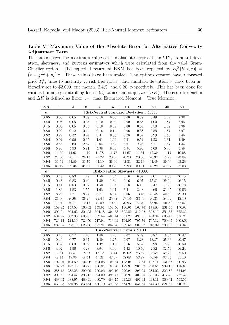
4.3 Alternative Convexity Adjustment Term
The errors of using the Black-Scholes return in place of BKM’s approximation have been
tabulated in Tables IV and V and presented in Figures 14 and 15.
[Insert Tables IV and V and Figures 14 and 15 about here.]
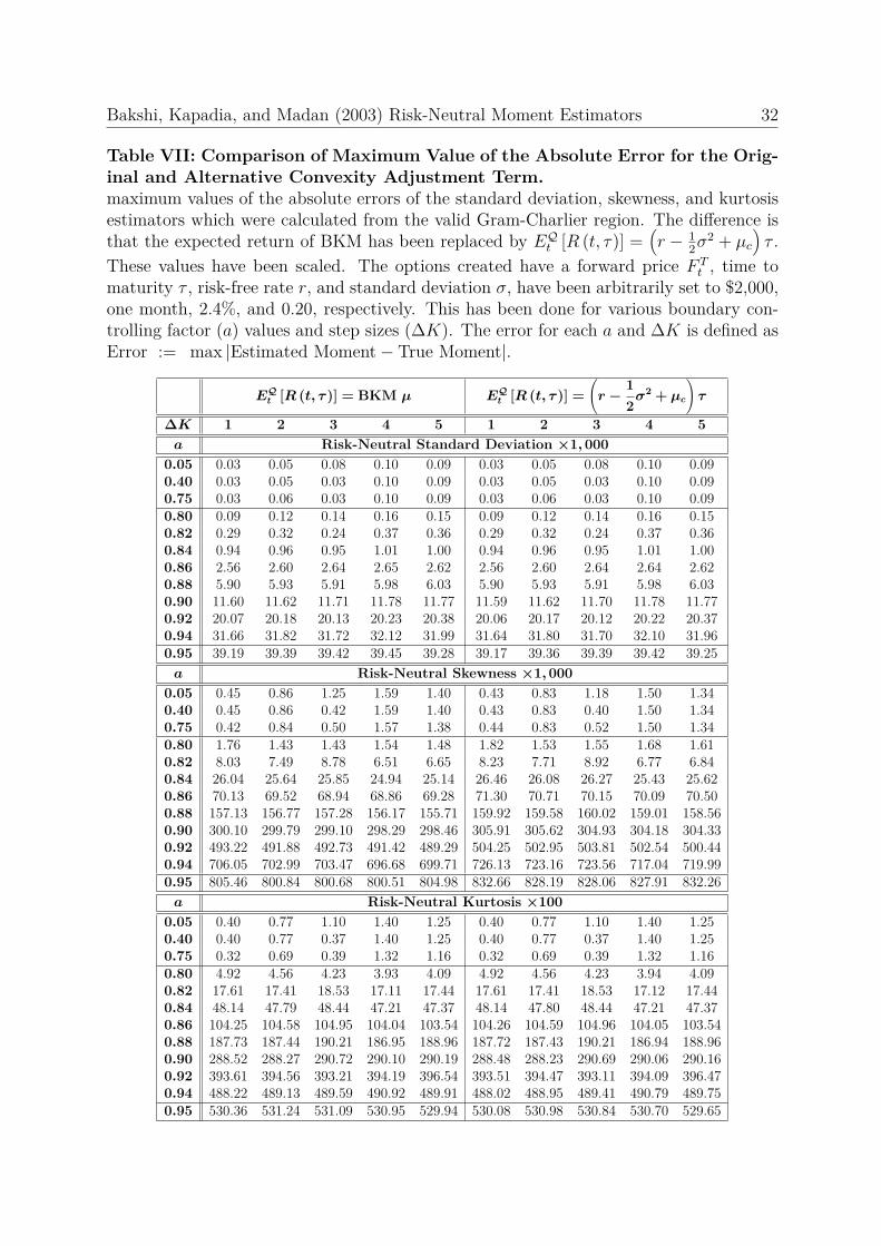
Tables IV and V have been combined with Tables II and III in Tables VI and VII,
respectively, to allow for ease of comparison.
[Insert Tables VI and VII about here.]
In general, there is a slight decrease in both mean and absolute maximum errors for
skewness when the boundary controlling factor is less than 0.75. For larger boundary
controlling factors, the alternate convexity adjustment term increases the errors.
5 Implications
The implications of this papers are that the discretised BKM methodology is unable to
accurately mainly due to the interval of strikes being too large. The truncation errors do
cause some issues; however, not as much as the step size (for the intervals used). Many
papers have studied the smoothing and extrapolation techniques which can be used to
improve the accuracy of the BKM estimators. This paper provides a way to compare
the estimator with the true underlying moment. Using this methodology, smoothing
techniques as well as extrapolating techniques can be remeasured using true moment
values.
6 Conclusion
This paper shows a method to create virtual options using the Gram-Charlier series. These
virtual options are created by specifying the mean, variance, skewness, and kurtosis. By
Bakshi, Kapadia, and Madan (2003) Risk-Neutral Moment Estimators 16
doing so, risk-neutral moment estimators can be compared with the true values. The
BKM method is used to calculate the CBOE SKEW, this paper finds that to estimate
skewness within 10−3 of the true value, the range of strikes (Kmin, Kmax) must contain at
least 3/4 to 4/3 of the forward price and have a step size (∆K) of no more than 0.1% of the
forward price. Rather than using the absolute error as the measure, if the average error
is used, then the step size restriction can be relaxed to 1% of the forward price. Under
the same boundary controlling factor and step size specification, the absolute errors of
the kurtosis, standard deviation and VIX are bounded by 5 × 10⁻³, 10−4, and 5 × 10⁻³,
respectively.
The errors of skewness were found to oscillate with respect to the step size. Increas-
ing the granularity of the step size decreases the error approximately quadratically, not
exponentially.

Bakshi, Kapadia, and Madan (2003) Risk-Neutral Moment Estimators 17
References
Backus, David K., Silverio Foresi, and Liuren Wu, 2004, Accounting for biases in Black-Scholes, Available at SSRN: https://ssrn.com/abstract=585623.
Bakshi, Gurdip, Nikunj Kapadia, and Dilip Madan, 2003, Stock return characteristics,skew laws, and the differential pricing of individual equity options, Review of FinancialStudies 16(1), 101–143.
Bakshi, Gurdip and Dilip Madan, 2006, A theory of volatility spreads, Management Sci-ence 52(12), 1945–1956.
Bates, David S., 1996, Jumps and stochastic volatility: Exchange rate processes implicitin Deutsche Mark options, Review of Financial Studies 9(1), 69–107.
Black, Fischer and Myron Scholes, 1973, The pricing of options and corporate liabilities,Journal of Political Economy 81(3), 637–654.
Carr, Peter and Dilip Madan, 2001a, Optimal positioning in derivative securities, Quan-titative Finance 1(1), 19–37.
Carr, Peter and Dilip Madan, 2001b, Towards a theory of volatility trading. Handbooks inmathematical finance: Option pricing, interest rates and risk management. CambridgeUniversity Press, 458–476.
Chang, Bo Young, Peter Christoffersen, and Kris Jacobs, 2013, Market skewness risk andthe cross section of stock returns, Journal of Financial Economics 107(1), 46–68.
Chang, Bo Young, Peter Christoffersen, Kris Jacobs, and Gregory Vainberg, 2011, Option-implied measures of equity risk, Review of Finance 16(2), 385–428.
Chatrath, Arjun, Hong Miao, Sanjay Ramchander, and Tianyang Wang, 2016, An exam-ination of the flow characteristics of crude oil: Evidence from risk-neutral moments,Energy Economics 54, 213–223.
Cheng, Ing-Haw, 2018, The VIX premium, Review of Financial Studies 32(1), 180–227.
Christoffersen, Peter, Kris Jacobs, and Bo Young Chang, 2011, Chapter 10 - forecastingwith option-implied information, Handbook of economic forecasting. Vol. 2. Elsevier,581–656.
Conrad, Jennifer, Robert F. Dittmar, and Eric Ghysels, 2013, Ex ante skewness andexpected stock returns, Journal of Finance 68(1), 85–124.
Bakshi, Kapadia, and Madan (2003) Risk-Neutral Moment Estimators 18
Demeterfi, Kresimir, Emanuel Derman, Michael Kamal, and Joseph Zou, 1999, A guideto volatility and variance swaps, Journal of Derivatives 6(4), 9–32.
Dennis, Patrick and Stewart Mayhew, 2002, Risk-neutral skewness: evidence from stockoptions, Journal of Financial and Quantitative Analysis 37(3), 471–493.
Harrison, John M. and David M. Kreps, 1979, Martingales and arbitrage in multiperiodsecurities markets, Journal of Economic Theory 20(3), 381–408.
Harrison, John M. and Stanley R. Pliska, 1981, Martingales and stochastic integrals inthe theory of continuous trading, Stochastic Processes and their Applications 11(3),215–260.
Heston, Steven L., 1993, A closed-form solution for options with stochastic volatility withapplications to bond and currency options, Review of Financial Studies 6(2), 327–343.
Jarrow, Robert and Andrew Rudd, 1982, Approximate option valuation for arbitrarystochastic processes, Journal of Financial Economics 10(3), 347–369.
Jiang, George J. and Yisong S. Tian, 2005, The model-free implied volatility and itsinformation content, Review of Financial Studies 18(4), 1305–1342.
Jiang, George J. and Yisong S. Tian, 2007, Extracting model-free volatility from optionprices, Journal of Derivatives 14(3), 35–60.
Jondeau, Eric and Michael Rockinger, 2001, Gram-Charlier densities, Journal of EconomicDynamics and Control 25(10), 1457–1483.
Lee, Geul and Li Yang, 2015, Impact of truncation on model-free implied moment esti-mator, Available at SSRN: https://ssrn.com/abstract=2485513.
Liu, Zhangxin and Robert Faff, 2017, Hitting SKEW for SIX, Economic Modelling 64,449–464.
Liu, Zhangxin and Thijs van der Heijden, 2016, Model-free risk-neutral moments andproxies, Available at SSRN: https://ssrn.com/abstract=2641559.
Longstaff, Francis A., 1995, Option pricing and the martingale restriction, Review ofFinancial Studies 8(4), 1091–1124.
Merton, Robert C., 1973, Theory of rational option pricing, Bell Journal of Economicsand Management Science 4(1), 141–183.
Bakshi, Kapadia, and Madan (2003) Risk-Neutral Moment Estimators 19
Merton, Robert C., 1976, Option pricing when underlying stock returns are discontinuous,Journal of Financial Economics 3(1), 125–144.
Neumann, Michael and George Skiadopoulos, 2013, Predictable dynamics in higher-orderrisk-neutral moments: Evidence from the S&P 500 options, Journal of Financial andQuantitative Analysis 48(3), 947–977.
Ruan, Xinfeng and Jin E. Zhang, 2018, Risk-neutral moments in the crude oil market,Energy Economics 72, 583–600.
Stilger, Przemysław S., Alexandros Kostakis, and Ser-Huang Poon, 2017, What does risk-neutral skewness tell us about future stock returns? Management Science 63(6), 1814–1834.
Zhang, Jin E. and Yi Xiang, 2008, The implied volatility smirk, Quantitative Finance8(3), 263–284.
Bakshi, Kapadia, and Madan (2003) Risk-Neutral Moment Estimators 20
Appendix
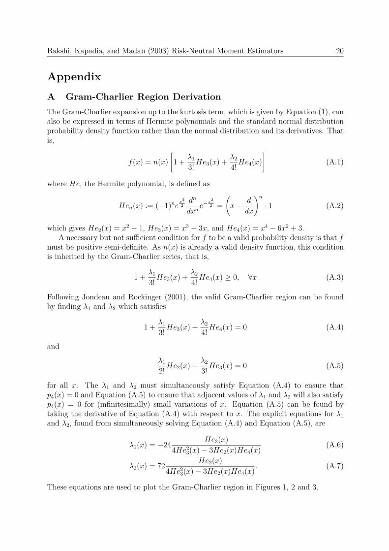
A Gram-Charlier Region DerivationThe Gram-Charlier expansion up to the kurtosis term, which is given by Equation (1), canalso be expressed in terms of Hermite polynomials and the standard normal distributionprobability density function rather than the normal distribution and its derivatives. Thatis,
f(x) = n(x)[1 + λ1
3!He3(x) + λ2
4!He4(x)]
(A.1)
where He, the Hermite polynomial, is defined as
Hen(x) := (−1)nex2
2dn
dxne−
x22 =
(x− d
dx
)n· 1 (A.2)
which gives He2(x) = x2 − 1, He3(x) = x3 − 3x, and He4(x) = x4 − 6x2 + 3.A necessary but not sufficient condition for f to be a valid probability density is that f
must be positive semi-definite. As n(x) is already a valid density function, this conditionis inherited by the Gram-Charlier series, that is,
1 + λ1
3!He3(x) + λ2
4!He4(x) ≥ 0, ∀x (A.3)
Following Jondeau and Rockinger (2001), the valid Gram-Charlier region can be foundby finding λ1 and λ2 which satisfies
1 + λ1
3!He3(x) + λ2
4!He4(x) = 0 (A.4)
and
λ1
2!He2(x) + λ2
3!He3(x) = 0 (A.5)
for all x. The λ1 and λ2 must simultaneously satisfy Equation (A.4) to ensure thatp4(x) = 0 and Equation (A.5) to ensure that adjacent values of λ1 and λ2 will also satisfyp4(x) = 0 for (infinitesimally) small variations of x. Equation (A.5) can be found bytaking the derivative of Equation (A.4) with respect to x. The explicit equations for λ1and λ2, found from simultaneously solving Equation (A.4) and Equation (A.5), are
λ1(x) = −24 He3(x)4He2
3(x)− 3He2(x)He4(x) (A.6)
λ2(x) = 72 He2(x)4He2
3(x)− 3He2(x)He4(x) . (A.7)
These equations are used to plot the Gram-Charlier region in Figures 1, 2 and 3.
Bakshi, Kapadia, and Madan (2003) Risk-Neutral Moment Estimators 21
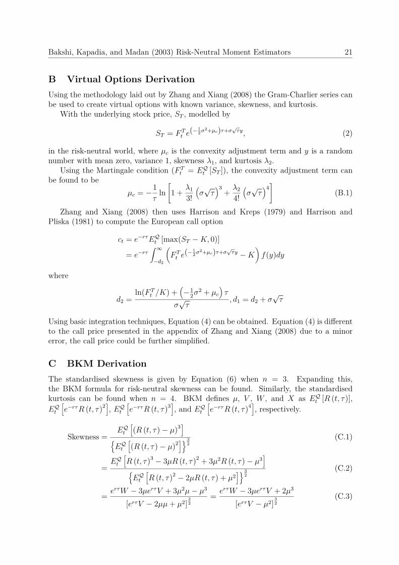
B Virtual Options DerivationUsing the methodology laid out by Zhang and Xiang (2008) the Gram-Charlier series canbe used to create virtual options with known variance, skewness, and kurtosis.
With the underlying stock price, ST , modelled by
ST = F Tt e
(− 12σ
2+µc)τ+σ√τy, (2)
in the risk-neutral world, where µc is the convexity adjustment term and y is a randomnumber with mean zero, variance 1, skewness λ1, and kurtosis λ2.
Using the Martingale condition (F Tt = EQt [ST ]), the convexity adjustment term can
be found to beµc = −1
τln[1 + λ1
3!(σ√τ)3
+ λ2
4!(σ√τ)4]
(B.1)
Zhang and Xiang (2008) then uses Harrison and Kreps (1979) and Harrison andPliska (1981) to compute the European call option
ct = e−rτEQt [max(ST −K, 0)]
= e−rτ∫ ∞−d2
(F Tt e
(− 12σ
2+µc)τ+σ√τy −K
)f(y)dy
where
d2 =ln(F T
t /K) +(−1
2σ2 + µc
)τ
σ√τ
, d1 = d2 + σ√τ
Using basic integration techniques, Equation (4) can be obtained. Equation (4) is differentto the call price presented in the appendix of Zhang and Xiang (2008) due to a minorerror, the call price could be further simplified.
C BKM DerivationThe standardised skewness is given by Equation (6) when n = 3. Expanding this,the BKM formula for risk-neutral skewness can be found. Similarly, the standardisedkurtosis can be found when n = 4. BKM defines µ, V , W , and X as EQt [R (t, τ)],EQt
[e−rτR (t, τ)2
], EQt
[e−rτR (t, τ)3
], and EQt
[e−rτR (t, τ)4
], respectively.
Skewness =EQt
[(R (t, τ)− µ)3
]EQt
[(R (t, τ)− µ)2
] 32
(C.1)
=EQt
[R (t, τ)3 − 3µR (t, τ)2 + 3µ2R (t, τ)− µ3
]EQt
[R (t, τ)2 − 2µR (t, τ) + µ2
] 32
(C.2)
= erτW − 3µerτV + 3µ2µ− µ3
[erτV − 2µµ+ µ2]32
= erτW − 3µerτV + 2µ3
[erτV − µ2]32
(C.3)

Bakshi, Kapadia, and Madan (2003) Risk-Neutral Moment Estimators 22
Kurtosis =EQt
[(R (t, τ)− µ)4
]EQt
[(R (t, τ)− µ)2
]2 (C.4)
=EQt
[R (t, τ)4 − 4µR (t, τ)3 + 6µ2R (t, τ)2 − 4µ3R (t, τ) + µ4
]EQt
[R (t, τ)2 − 2µR (t, τ) + µ2
]2 (C.5)
= erτX − 4µerτW + 6µ2erτV − 4µ3µ+ µ4
[erτV − 2µµ+ µ2]2(C.6)
= erτX − 4µerτW + 6µ2erτV − 3µ4
[erτV − µ2]2(C.7)
The (annualized) variance σ2 is given by
σ2 = 1τEQt
[(R (t, τ)− µ)2
]= erτV − µ2
τ(C.8)
D Numerical IntegrationThe traditional trapezium rule is given in the form of Equation (D.1). With a smallrearrangement, Equation (D.2) can be obtained. This is the trapezium rule that is usedfor calculations.∫ b
af(x)dx =
n−1∑i=1
f(xi) + f(xi+1)2 ∆xi, ∆xi = xi+1 − xi (D.1)
=n∑i=1
f(xi)∆xi, ∆xi = 12
x2 − x1, i = 1xi+1 − xi−1, 1 < i < n
xn − xn−1, i = n
(D.2)
The CBOE uses Equation (D.3) which introduces a small error at the end points, Kminand Kmax. This method does, however, give equal weighting to each option - rather thanhalf the weight given to end points if the traditional trapezium rule is used.
∫ b
af(x)dx ≈
n∑i=1
f(xi)∆xi, ∆xi =
x2 − x1, i = 1xi+1−xi−1
2 , 1 < i < n
xn − xn−1, i = n
(D.3)
=∫ b
af(x)dx−
(f(x1)x2 − x1
2 + f(xn)xn − xn−1
2
)(D.4)

Bakshi, Kapadia, and Madan (2003) Risk-Neutral Moment Estimators 23
E VIX DerivationE.1 Variance Swap Derivation
Demeterfi, Derman, Kamal, and Zou (1999) present a method to replicate variance swapswith European options. Following part of their procedure, for a differential stock priceform of
dStSt
= (r − q) dt+ σtdWt
where r, q and σ is risk-free rate, continuous dividend rate and the volatility parameters,respectively, the following can be obtained:
VIX2 = 2τEQt
[∫ T
t
dStSt− ln ST
St
]× 1002 (E.1)
With some algebraic manipulation, an intuitive formula can be found:
VIX = 100√−2τEQt
[ln STSte(r−q)τ
](E.2)
E.2 CBOE VIX
Using the integral form of stock price derived using the Gram-Charlier region, with somealgebra, the following can be obtained.
VIX2 = −2τEQt
[ln STSte(r−q)τ
]× 1002 (E.3)
= −2τEQt
[(−1
2σ2 + µc
)τ + σ
√τy]× 1002 (E.4)
=[(σ2 − 2µc
)− 2τσ√τEQt [y]
]× 1002 (E.5)
=[σ2 − 2µc
]× 1002 (E.6)
=⇒ VIX = 100√σ2 − 2µc (E.7)
The volatility index can also calculated using the BKM method
VIX2 = −2τEQt
[ln STSterτ
]× 1002 =
[−2τEQt [R (t, τ)] + 2r
]× 1002 (E.8)
=⇒ VIX ≈ 100√−2τµ+ 2r (E.9)
where
µ(t, τ) := erτ − 1− 12EQt
[R (t, τ)2
]− 1
3!EQt
[R (t, τ)3
]− 1
4!EQt
[R (t, τ)4
](E.10)
As µ, the approximation of EQt [R (t, τ)], is required, this method introduces errors, how-ever, it does remain model-free.

Bakshi, Kapadia, and Madan (2003) Risk-Neutral Moment Estimators 24
F BKM and Black-Scholes Risk-Neutral Log ReturnsUsing the standard Black-Scholes stock price model,
ST = Ste(r− 1
2σ2)τ+σWτ , (F.1)
where Wτ is a Wiener process, the expected value of log returns is
EQt [R (t, τ)] = EQt
[(r − 1
2σ2)τ + σWτ
]=(r − 1
2σ2)τ. (F.2)
From this, the BKM’s approximation can be compared like so
EQt [R (t, τ)] ≈ erτ − 1− 12EQt
[R (t, τ)2
]− 1
3!EQt
[R (t, τ)3
]− 1
4!EQt
[R (t, τ)4
].
As the BKM approximates the exponential term when used with R(t, τ), this is also doneto erτ . The result is
EQt [R (t, τ)] ≈ 1 + rτ + 12(rτ)2 + 1
3!(rτ)3 + 14!(rτ)4 − 1
− 12EQt
[R (t, τ)2
]− 1
3!EQt
[R (t, τ)3
]− 1
4!EQt
[R (t, τ)4
].
Expanding this further and simplifying, Equation (23) can be obtained.
G Error Envelope DerivationUsing a simple curve was sufficient to capture the main characteristics of the error.
Y = Errors (Peaks (+ or −)) (G.1)x = Corresponding ∆K (G.2)X =
[x x2
](G.3)
For y = β1x+ β2x2
Y = Xβ (G.4)
=⇒ β =(XTX
)−1XTY (G.5)
For the positive envelope and negative envelope, the coefficients are assigned to β+ andβ−, respectively. The symmetric envelope and trend can be found from βs = β+−β−
2 andβt = β++β−
2 , respectively. From this, the envelope component equations are given by
Es = Xβs (G.6)Et = Xβt (G.7)
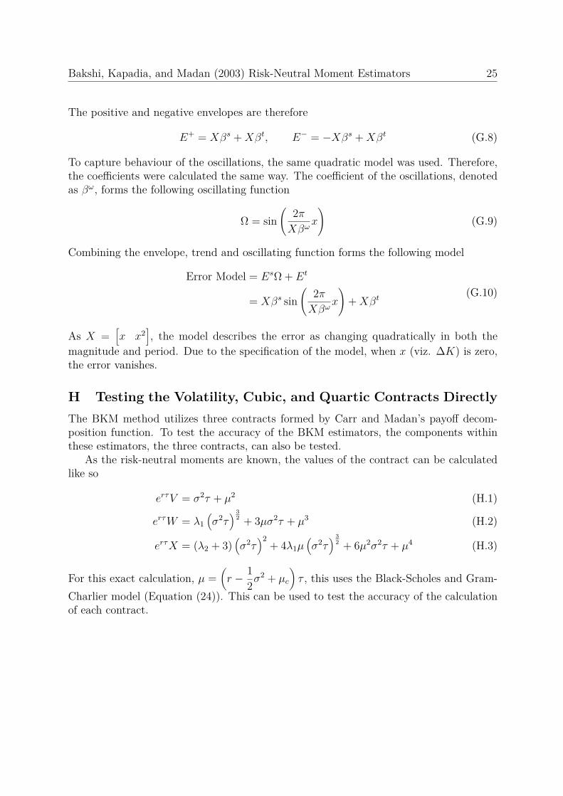
Bakshi, Kapadia, and Madan (2003) Risk-Neutral Moment Estimators 25
The positive and negative envelopes are therefore
E+ = Xβs +Xβt, E− = −Xβs +Xβt (G.8)
To capture behaviour of the oscillations, the same quadratic model was used. Therefore,the coefficients were calculated the same way. The coefficient of the oscillations, denotedas βω, forms the following oscillating function
Ω = sin(
2πXβω
x
)(G.9)
Combining the envelope, trend and oscillating function forms the following model
Error Model = EsΩ + Et
= Xβs sin(
2πXβω
x
)+Xβt
(G.10)
As X =[x x2
], the model describes the error as changing quadratically in both the
magnitude and period. Due to the specification of the model, when x (viz. ∆K) is zero,the error vanishes.
H Testing the Volatility, Cubic, and Quartic Contracts DirectlyThe BKM method utilizes three contracts formed by Carr and Madan’s payoff decom-position function. To test the accuracy of the BKM estimators, the components withinthese estimators, the three contracts, can also be tested.
As the risk-neutral moments are known, the values of the contract can be calculatedlike so
erτV = σ2τ + µ2 (H.1)
erτW = λ1(σ2τ
) 32 + 3µσ2τ + µ3 (H.2)
erτX = (λ2 + 3)(σ2τ
)2+ 4λ1µ
(σ2τ
) 32 + 6µ2σ2τ + µ4 (H.3)
For this exact calculation, µ =(r − 1
2σ2 + µc
)τ , this uses the Black-Scholes and Gram-
Charlier model (Equation (24)). This can be used to test the accuracy of the calculationof each contract.
Bakshi, Kapadia, and Madan (2003) Risk-Neutral Moment Estimators 26
Tables
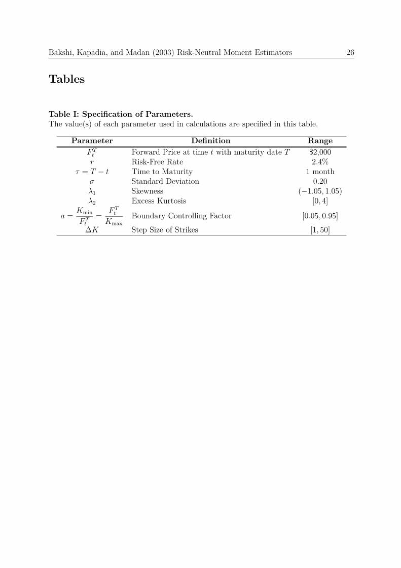
Table I: Specification of Parameters.The value(s) of each parameter used in calculations are specified in this table.
Parameter Definition RangeF Tt Forward Price at time t with maturity date T $2,000r Risk-Free Rate 2.4%
τ = T − t Time to Maturity 1 monthσ Standard Deviation 0.20λ1 Skewness (−1.05, 1.05)λ2 Excess Kurtosis [0, 4]
a = Kmin
F Tt
= F Tt
KmaxBoundary Controlling Factor [0.05, 0.95]
∆K Step Size of Strikes [1, 50]
Bakshi, Kapadia, and Madan (2003) Risk-Neutral Moment Estimators 27
Table II: Lookup Table for Mean Errors.This table shows the mean errors of the VIX, standard deviation, skewness, and kur-tosis estimators which were calculated from the valid Gram-Charlier region. These val-ues have been scaled. The options created have a forward price F T
t , time to maturityτ , risk-free rate r, and standard deviation σ, have been arbitrarily set to $2,000, onemonth, 2.4%, and 0.20, respectively. This has been done for various boundary control-ling factor (a) values and step sizes (∆K). The error for each a and ∆K is defined asError := mean (Estimated Moment− True Moment).
∆K 1 2 3 4 5 10 20 30 40 50a VIX ×10
0.05 -0.03 -0.06 -0.08 -0.10 -0.09 0.00 0.38 -0.49 -1.12 2.980.40 -0.03 -0.06 0.03 -0.10 -0.09 0.00 0.38 1.00 1.87 2.980.75 -0.03 -0.06 -0.03 -0.10 -0.09 0.00 0.38 -0.50 -1.12 2.980.80 -0.06 -0.09 -0.11 -0.13 -0.12 -0.03 0.35 -0.53 1.82 2.940.82 -0.17 -0.20 -0.12 -0.25 -0.24 -0.15 0.20 0.82 1.62 -0.260.84 -0.53 -0.55 -0.54 -0.60 -0.59 -0.49 -0.13 -1.07 1.22 -2.040.86 -1.44 -1.48 -1.52 -1.53 -1.50 -1.48 -1.11 -2.01 0.34 -3.110.88 -3.42 -3.45 -3.42 -3.50 -3.54 -3.45 -3.37 -2.49 -2.62 -3.930.90 -7.04 -7.06 -7.14 -7.21 -7.20 -7.11 -6.75 -7.71 -6.40 -5.340.92 -13.13 -13.24 -13.18 -13.29 -13.44 -13.35 -13.89 -14.01 -12.48 -16.770.94 -22.97 -23.14 -23.05 -23.49 -23.33 -23.99 -23.66 -23.10 -22.32 -34.920.95 -30.20 -30.42 -30.45 -30.48 -30.28 -31.18 -30.87 -36.88 -33.17 -28.67a Risk-Neutral Standard Deviation ×1,000
0.05 -0.03 -0.05 -0.08 -0.10 -0.09 0.00 0.38 -0.49 -1.12 2.980.40 -0.03 -0.05 0.03 -0.10 -0.09 0.00 0.38 1.00 1.87 2.980.75 -0.03 -0.06 -0.03 -0.10 -0.09 0.00 0.38 -0.50 -1.12 2.980.80 -0.06 -0.09 -0.11 -0.13 -0.12 -0.03 0.34 -0.52 1.82 2.940.82 -0.17 -0.20 -0.12 -0.25 -0.24 -0.15 0.20 0.82 1.63 -0.230.84 -0.53 -0.56 -0.54 -0.60 -0.59 -0.50 -0.13 -1.07 1.24 -2.040.86 -1.45 -1.49 -1.52 -1.53 -1.51 -1.48 -1.11 -2.01 0.33 -3.120.88 -3.43 -3.46 -3.42 -3.51 -3.54 -3.45 -3.34 -2.49 -2.51 -3.920.90 -7.05 -7.08 -7.14 -7.21 -7.20 -7.11 -6.75 -7.72 -6.30 -5.240.92 -13.13 -13.23 -13.18 -13.28 -13.42 -13.33 -13.80 -13.99 -12.39 -16.510.94 -22.96 -23.12 -23.03 -23.45 -23.30 -23.92 -23.58 -23.03 -22.25 -34.430.95 -30.19 -30.40 -30.43 -30.46 -30.27 -31.12 -30.80 -36.60 -33.10 -28.61a Risk-Neutral Skewness ×1,000
0.05 -0.02 -0.04 -0.07 -0.09 -0.07 0.09 0.75 -2.09 -1.99 5.420.40 -0.02 -0.04 0.02 -0.09 -0.07 0.09 0.75 1.84 3.40 5.420.75 -0.01 -0.03 -0.01 -0.08 -0.06 0.10 0.76 0.49 -1.97 5.430.80 0.76 0.73 0.71 0.69 0.71 0.88 1.58 -1.17 3.39 6.540.82 2.57 2.41 2.48 2.08 1.95 1.35 0.26 1.51 -1.56 -15.760.84 6.41 6.39 6.01 6.35 6.38 6.58 7.39 3.16 1.35 1.430.86 13.68 12.77 11.85 12.74 13.66 9.29 10.11 7.71 13.44 12.450.88 22.95 22.94 19.67 22.92 19.62 19.81 3.04 21.76 -33.26 11.790.90 33.81 33.80 28.57 28.54 28.55 28.70 29.27 29.62 -24.08 -21.350.92 39.19 35.34 39.18 35.32 27.55 27.68 -12.32 25.22 -9.41 -116.200.94 44.68 39.06 39.05 27.64 33.38 4.35 4.90 5.83 7.17 -312.590.95 48.46 41.53 41.53 41.52 48.46 13.17 13.59 -154.54 9.59 16.90a Risk-Neutral Kurtosis ×100
0.05 0.30 0.57 0.81 1.03 0.92 -0.05 -3.90 5.06 11.85 -29.910.40 0.30 0.57 -0.27 1.03 0.92 -0.05 -3.90 -10.23 -18.95 -29.910.75 0.25 0.52 0.30 0.99 0.87 -0.10 -3.95 5.18 11.79 -29.980.80 -2.72 -2.45 -2.20 -1.98 -2.10 -3.08 -6.96 1.86 -22.85 -33.190.82 -10.04 -9.86 -10.69 -9.59 -9.81 -11.28 -16.28 -22.69 -34.26 -18.720.84 -28.07 -27.82 -28.24 -27.38 -27.50 -28.46 -32.31 -26.23 -52.06 -15.070.86 -62.21 -62.36 -62.55 -61.95 -61.67 -64.59 -68.21 -60.58 -82.37 -51.650.88 -114.83 -114.61 -116.48 -114.24 -115.53 -116.33 -125.57 -124.74 -150.27 -122.660.90 -181.35 -181.16 -182.81 -182.33 -182.41 -183.05 -185.60 -179.00 -210.07 -217.060.92 -255.47 -256.14 -255.16 -255.86 -257.57 -258.03 -267.91 -254.03 -274.90 -278.010.94 -328.86 -329.59 -329.96 -331.04 -330.22 -334.64 -335.65 -337.35 -339.77 -342.570.95 -364.12 -364.86 -364.74 -364.63 -363.78 -368.12 -368.65 -376.61 -357.58 -372.80

Bakshi, Kapadia, and Madan (2003) Risk-Neutral Moment Estimators 28
Table III: Lookup Table for Maximum Absolute Errors.This table shows the maximum values of the absolute errors of the VIX, standard de-viation, skewness, and kurtosis estimators which were calculated from the valid Gram-Charlier region. These values have been scaled. The options created have a forward priceF Tt , time to maturity τ , risk-free rate r, and standard deviation σ, have been arbitrarily
set to $2,000, one month, 2.4%, and 0.20, respectively. This has been done for variousboundary controlling factor (a) values and step sizes (∆K). The error for each a and ∆Kis defined as Error := max |Estimated Moment− True Moment|.
∆K 1 2 3 4 5 10 20 30 40 50a VIX ×10
0.05 0.03 0.06 0.08 0.10 0.09 0.01 0.39 0.49 1.13 3.010.40 0.03 0.06 0.03 0.10 0.09 0.01 0.39 1.01 1.89 3.010.75 0.03 0.06 0.04 0.10 0.09 0.01 0.39 0.50 1.13 3.010.80 0.09 0.12 0.14 0.16 0.15 0.06 0.38 0.56 1.87 2.990.82 0.29 0.31 0.23 0.37 0.36 0.28 0.37 0.99 1.85 0.510.84 0.92 0.94 0.93 0.99 0.98 0.89 0.52 1.52 1.81 2.480.86 2.51 2.56 2.61 2.61 2.57 2.59 2.23 3.15 1.68 4.300.88 5.82 5.85 5.85 5.89 5.97 5.88 5.98 4.93 5.74 6.610.90 11.45 11.48 11.60 11.67 11.66 11.57 11.21 12.20 11.39 10.300.92 19.89 20.03 19.95 20.08 20.29 20.19 20.94 20.84 19.43 24.530.94 31.46 31.65 31.55 32.02 31.85 32.57 32.18 31.55 30.66 44.520.95 38.99 39.22 39.25 39.28 39.07 39.98 39.61 45.94 41.88 37.03a Risk-Neutral Standard Deviation ×1,000
0.05 0.03 0.05 0.08 0.10 0.09 0.00 0.38 0.49 1.12 2.980.40 0.03 0.05 0.03 0.10 0.09 0.00 0.38 1.00 1.87 2.980.75 0.03 0.06 0.03 0.10 0.09 0.00 0.38 0.50 1.12 2.980.80 0.09 0.12 0.14 0.16 0.15 0.06 0.38 0.55 1.87 2.970.82 0.29 0.32 0.24 0.37 0.36 0.28 0.37 0.99 1.85 0.450.84 0.94 0.96 0.95 1.01 1.00 0.91 0.54 1.52 1.81 2.490.86 2.56 2.60 2.64 2.65 2.62 2.61 2.25 3.17 1.67 4.340.88 5.90 5.93 5.91 5.98 6.03 5.94 5.93 5.00 5.47 6.590.90 11.60 11.62 11.71 11.78 11.77 11.68 11.32 12.31 11.17 10.090.92 20.07 20.18 20.13 20.23 20.38 20.29 20.82 20.93 19.30 23.860.94 31.66 31.82 31.72 32.12 31.99 32.53 32.15 31.51 30.62 43.310.95 39.19 39.39 39.42 39.45 39.28 40.01 39.64 45.26 41.90 37.05a Risk-Neutral Skewness ×1,000
0.05 0.45 0.86 1.25 1.59 1.40 0.17 6.40 9.43 18.97 48.730.40 0.45 0.86 0.42 1.59 1.40 0.17 6.40 16.69 30.87 48.730.75 0.42 0.84 0.50 1.57 1.38 0.19 6.43 8.04 18.94 48.760.80 1.76 1.43 1.43 1.54 1.48 2.40 8.72 7.12 32.85 51.590.82 8.03 7.49 8.78 6.51 6.65 7.95 13.66 24.23 39.40 29.680.84 26.04 25.64 25.85 24.94 25.14 26.78 33.32 19.46 56.10 10.000.86 70.13 69.52 68.94 68.86 69.28 69.78 76.37 62.33 102.23 54.460.88 157.13 156.77 157.28 156.17 155.71 157.29 160.27 173.96 233.88 167.690.90 300.10 299.79 299.10 298.29 298.46 299.80 305.14 295.80 359.97 369.990.92 493.22 491.88 492.73 491.42 489.29 490.18 511.61 482.16 519.22 641.210.94 706.05 702.99 703.47 696.68 699.71 685.77 685.68 687.45 690.14 1041.570.95 805.46 800.84 800.68 800.51 804.98 781.73 781.60 954.29 760.23 781.10a Risk-Neutral Kurtosis ×100
0.05 0.40 0.77 1.10 1.40 1.25 0.07 5.28 6.87 16.04 40.480.40 0.40 0.77 0.37 1.40 1.25 0.07 5.28 13.87 25.67 40.480.75 0.32 0.69 0.39 1.32 1.16 0.16 5.38 6.98 15.93 40.600.80 4.92 4.56 4.23 3.93 4.09 5.42 10.69 2.83 32.55 46.250.82 17.61 17.41 18.53 17.11 17.44 19.62 26.82 35.53 52.24 32.520.84 48.14 47.79 48.44 47.21 47.37 48.67 53.87 46.59 82.06 31.100.86 104.25 104.58 104.95 104.04 103.54 108.04 112.82 102.70 131.53 90.920.88 187.73 187.44 190.21 186.95 188.96 189.97 203.51 200.64 239.27 198.810.90 288.52 288.27 290.72 290.10 290.19 290.95 293.97 285.05 326.85 334.870.92 393.61 394.56 393.21 394.19 396.54 397.03 409.88 391.09 417.34 422.370.94 488.22 489.13 489.59 490.92 489.91 495.30 496.35 498.13 500.66 503.970.95 530.36 531.24 531.09 530.95 529.94 535.06 535.65 544.30 521.68 540.33

Bakshi, Kapadia, and Madan (2003) Risk-Neutral Moment Estimators 29
Table IV: Errors for Alternative Convexity Adjustment Term.This table shows the mean errors of the VIX, standard deviation, skewness, and kur-tosis estimators which were calculated from the valid Gram-Charlier region. The ex-pected return of BKM has been replaced by EQt [R (t, τ)] =
(r − 1
2σ2 + µc
)τ . These
values have been scaled. The options created have a forward price F Tt , time to maturity
τ , risk-free rate r, and standard deviation σ, have been arbitrarily set to $2,000, onemonth, 2.4%, and 0.20, respectively. This has been done for various boundary control-ling factor (a) values and step sizes (∆K). The error for each a and ∆K is defined asError := mean (Estimated Moment− True Moment).
∆K 1 2 3 4 5 10 20 30 40 50a Risk-Neutral Standard Deviation ×1,000
0.05 -0.03 -0.05 -0.08 -0.10 -0.09 0.00 0.38 -0.49 -1.12 2.980.40 -0.03 -0.05 0.03 -0.10 -0.09 0.00 0.38 1.00 1.87 2.980.75 -0.03 -0.06 -0.03 -0.10 -0.09 0.00 0.38 -0.50 -1.12 2.980.80 -0.06 -0.09 -0.11 -0.13 -0.12 -0.03 0.34 -0.52 1.82 2.940.82 -0.17 -0.20 -0.12 -0.25 -0.24 -0.15 0.20 0.82 1.63 -0.230.84 -0.53 -0.56 -0.54 -0.60 -0.59 -0.50 -0.13 -1.07 1.24 -2.040.86 -1.45 -1.49 -1.52 -1.53 -1.51 -1.48 -1.11 -2.01 0.33 -3.120.88 -3.43 -3.46 -3.42 -3.51 -3.54 -3.45 -3.34 -2.49 -2.51 -3.920.90 -7.05 -7.07 -7.14 -7.21 -7.20 -7.11 -6.75 -7.71 -6.30 -5.240.92 -13.12 -13.23 -13.18 -13.28 -13.42 -13.33 -13.79 -13.98 -12.39 -16.500.94 -22.95 -23.11 -23.02 -23.44 -23.29 -23.90 -23.57 -23.01 -22.24 -34.400.95 -30.17 -30.38 -30.41 -30.44 -30.25 -31.10 -30.78 -36.57 -33.08 -28.59a Risk-Neutral Skewness ×1,000
0.05 0.00 0.00 0.00 -0.00 0.01 0.09 0.42 -1.67 -1.01 2.860.40 0.00 0.00 0.00 -0.00 0.01 0.09 0.42 0.98 1.78 2.860.75 0.02 0.02 0.02 0.01 0.02 0.10 0.43 0.93 -1.00 2.870.80 0.81 0.81 0.81 0.81 0.82 0.91 1.28 -0.71 1.81 4.010.82 2.72 2.58 2.58 2.29 2.16 1.48 0.09 0.81 -2.96 -15.530.84 6.86 6.87 6.48 6.87 6.89 7.01 7.50 4.09 0.30 3.200.86 14.93 14.06 13.17 14.07 14.97 10.57 11.08 9.47 13.15 15.170.88 25.95 25.96 22.66 25.98 22.72 22.82 5.98 23.93 -30.97 15.240.90 40.03 40.04 34.88 34.91 34.92 34.98 35.23 36.45 -18.43 -16.650.92 50.99 47.24 51.03 47.27 39.65 39.69 0.20 37.85 1.80 -100.970.94 65.92 60.47 60.37 49.38 54.97 26.60 26.81 27.19 27.77 -279.030.95 76.99 70.30 70.33 70.35 77.08 42.73 42.82 -118.90 41.23 43.85a Risk-Neutral Kurtosis ×100
0.05 0.30 0.57 0.81 1.03 0.92 -0.05 -3.89 5.06 11.85 -29.910.40 0.30 0.57 -0.27 1.03 0.92 -0.05 -3.89 -10.23 -18.95 -29.910.75 0.25 0.52 0.30 0.99 0.87 -0.10 -3.95 5.18 11.79 -29.970.80 -2.72 -2.45 -2.20 -1.98 -2.10 -3.08 -6.96 1.86 -22.85 -33.180.82 -10.04 -9.87 -10.69 -9.60 -9.81 -11.28 -16.28 -22.69 -34.26 -18.720.84 -28.07 -27.82 -28.24 -27.38 -27.50 -28.46 -32.31 -26.24 -52.05 -15.080.86 -62.21 -62.37 -62.55 -61.96 -61.67 -64.59 -68.21 -60.58 -82.37 -51.660.88 -114.83 -114.61 -116.48 -114.24 -115.53 -116.33 -125.58 -124.75 -150.27 -122.670.90 -181.34 -181.15 -182.80 -182.32 -182.40 -183.04 -185.60 -178.99 -210.09 -217.070.92 -255.44 -256.11 -255.13 -255.82 -257.54 -258.01 -267.94 -254.01 -274.92 -278.240.94 -328.76 -329.50 -329.87 -330.98 -330.15 -334.64 -335.65 -337.35 -339.76 -343.960.95 -363.95 -364.71 -364.59 -364.48 -363.61 -368.08 -368.60 -377.34 -357.55 -372.74
Bakshi, Kapadia, and Madan (2003) Risk-Neutral Moment Estimators 30
Table V: Maximum Value of the Absolute Error for Alternative ConvexityAdjustment Term.This table shows the maximum values of the absolute errors of the VIX, standard devi-ation, skewness, and kurtosis estimators which were calculated from the valid Gram-Charlier region. The expected return of BKM has been replaced by EQt [R (t, τ)] =(r − 1
2σ2 + µc
)τ . These values have been scaled. The options created have a forward
price F Tt , time to maturity τ , risk-free rate r, and standard deviation σ, have been ar-
bitrarily set to $2,000, one month, 2.4%, and 0.20, respectively. This has been done forvarious boundary controlling factor (a) values and step sizes (∆K). The error for each aand ∆K is defined as Error := max |Estimated Moment− True Moment|.
∆K 1 2 3 4 5 10 20 30 40 50a Risk-Neutral Standard Deviation ×1,000
0.05 0.03 0.05 0.08 0.10 0.09 0.00 0.38 0.49 1.12 2.980.40 0.03 0.05 0.03 0.10 0.09 0.00 0.38 1.00 1.87 2.980.75 0.03 0.06 0.03 0.10 0.09 0.00 0.38 0.50 1.12 2.980.80 0.09 0.12 0.14 0.16 0.15 0.06 0.38 0.55 1.87 2.970.82 0.29 0.32 0.24 0.37 0.36 0.28 0.37 0.99 1.85 0.450.84 0.94 0.96 0.95 1.01 1.00 0.91 0.54 1.52 1.81 2.490.86 2.56 2.60 2.64 2.64 2.62 2.61 2.25 3.17 1.67 4.340.88 5.90 5.93 5.91 5.98 6.03 5.94 5.93 5.00 5.46 6.580.90 11.59 11.62 11.70 11.78 11.77 11.67 11.31 12.30 11.17 10.080.92 20.06 20.17 20.12 20.22 20.37 20.28 20.80 20.92 19.29 23.840.94 31.64 31.80 31.70 32.10 31.96 32.51 32.13 31.49 30.60 43.280.95 39.17 39.36 39.39 39.42 39.25 39.98 39.61 45.22 41.87 37.03a Risk-Neutral Skewness ×1,000
0.05 0.43 0.83 1.18 1.50 1.34 0.16 6.07 9.01 18.00 46.150.40 0.43 0.83 0.40 1.50 1.34 0.16 6.07 15.81 29.24 46.150.75 0.44 0.83 0.52 1.50 1.34 0.18 6.10 8.47 17.96 46.180.80 1.82 1.53 1.55 1.68 1.61 2.44 8.43 6.66 31.25 49.060.82 8.23 7.71 8.92 6.77 6.84 8.06 13.46 23.48 40.68 29.300.84 26.46 26.08 26.27 25.43 25.62 27.18 33.39 20.33 54.92 12.100.86 71.30 70.71 70.15 70.09 70.50 70.93 77.20 63.96 101.80 57.070.88 159.92 159.58 160.02 159.01 158.56 160.06 162.76 175.88 231.40 170.680.90 305.91 305.62 304.93 304.18 304.33 305.59 310.62 302.15 354.32 365.290.92 504.25 502.95 503.81 502.54 500.44 501.25 499.51 493.84 508.41 625.210.94 726.13 723.16 723.56 717.04 719.99 704.95 705.76 707.12 709.05 1005.640.95 832.66 828.19 828.06 827.91 832.26 809.53 809.07 918.02 790.09 806.32a Risk-Neutral Kurtosis ×100
0.05 0.40 0.77 1.10 1.40 1.25 0.07 5.28 6.87 16.04 40.470.40 0.40 0.77 0.37 1.40 1.25 0.07 5.28 13.87 25.66 40.470.75 0.32 0.69 0.39 1.32 1.16 0.16 5.37 6.98 15.93 40.590.80 4.92 4.56 4.23 3.94 4.09 5.42 10.69 2.82 32.54 46.240.82 17.61 17.41 18.53 17.12 17.44 19.62 26.82 35.52 52.28 32.500.84 48.14 47.80 48.44 47.21 47.37 48.68 53.87 46.59 82.05 31.190.86 104.26 104.59 104.96 104.05 103.54 108.05 112.83 102.71 131.53 90.930.88 187.72 187.43 190.21 186.94 188.96 189.97 203.52 200.64 239.15 198.820.90 288.48 288.23 290.69 290.06 290.16 290.91 293.93 285.02 326.87 334.930.92 393.51 394.47 393.11 394.09 396.47 396.97 409.96 391.03 417.40 422.370.94 488.02 488.95 489.41 490.79 489.75 495.28 496.33 498.11 500.64 505.500.95 530.08 530.98 530.84 530.70 529.65 534.97 535.55 545.30 521.61 540.23

Bakshi, Kapadia, and Madan (2003) Risk-Neutral Moment Estimators 31
Table VI: Comparison of Errors for the Original and Alternative ConvexityAdjustment Term.This table shows a comparison of the mean errors of the standard deviation, skewness,and kurtosis estimators which were calculated from the valid Gram-Charlier region. Thedifference is that the expected return of BKM has been replaced by EQt [R (t, τ)] =(r − 1
2σ2 + µc
)τ . These values have been scaled. The options created have a forward
price F Tt , time to maturity τ , risk-free rate r, and standard deviation σ, have been ar-
bitrarily set to $2,000, one month, 2.4%, and 0.20, respectively. This has been done forvarious boundary controlling factor (a) values and step sizes (∆K). The error for each aand ∆K is defined as Error := mean (Estimated Moment− True Moment).
EQt [R (t, τ )] = BKM µ EQt [R (t, τ )] =(r−
12σ2 + µc
)τ
∆K 1 2 3 4 5 1 2 3 4 5a Risk-Neutral Standard Deviation ×1,000
0.05 -0.03 -0.05 -0.08 -0.10 -0.09 -0.03 -0.05 -0.08 -0.10 -0.090.40 -0.03 -0.05 0.03 -0.10 -0.09 -0.03 -0.05 0.03 -0.10 -0.090.75 -0.03 -0.06 -0.03 -0.10 -0.09 -0.03 -0.06 -0.03 -0.10 -0.090.80 -0.06 -0.09 -0.11 -0.13 -0.12 -0.06 -0.09 -0.11 -0.13 -0.120.82 -0.17 -0.20 -0.12 -0.25 -0.24 -0.17 -0.20 -0.12 -0.25 -0.240.84 -0.53 -0.56 -0.54 -0.60 -0.59 -0.53 -0.56 -0.54 -0.60 -0.590.86 -1.45 -1.49 -1.52 -1.53 -1.51 -1.45 -1.49 -1.52 -1.53 -1.510.88 -3.43 -3.46 -3.42 -3.51 -3.54 -3.43 -3.46 -3.42 -3.51 -3.540.90 -7.05 -7.08 -7.14 -7.21 -7.20 -7.05 -7.07 -7.14 -7.21 -7.200.92 -13.13 -13.23 -13.18 -13.28 -13.42 -13.12 -13.23 -13.18 -13.28 -13.420.94 -22.96 -23.12 -23.03 -23.45 -23.30 -22.95 -23.11 -23.02 -23.44 -23.290.95 -30.19 -30.40 -30.43 -30.46 -30.27 -30.17 -30.38 -30.41 -30.44 -30.25a Risk-Neutral Skewness ×1,000
0.05 -0.02 -0.04 -0.07 -0.09 -0.07 0.00 0.00 0.00 -0.00 0.010.40 -0.02 -0.04 0.02 -0.09 -0.07 0.00 0.00 0.00 -0.00 0.010.75 -0.01 -0.03 -0.01 -0.08 -0.06 0.02 0.02 0.02 0.01 0.020.80 0.76 0.73 0.71 0.69 0.71 0.81 0.81 0.81 0.81 0.820.82 2.57 2.41 2.48 2.08 1.95 2.72 2.58 2.58 2.29 2.160.84 6.41 6.39 6.01 6.35 6.38 6.86 6.87 6.48 6.87 6.890.86 13.68 12.77 11.85 12.74 13.66 14.93 14.06 13.17 14.07 14.970.88 22.95 22.94 19.67 22.92 19.62 25.95 25.96 22.66 25.98 22.720.90 33.81 33.80 28.57 28.54 28.55 40.03 40.04 34.88 34.91 34.920.92 39.19 35.34 39.18 35.32 27.55 50.99 47.24 51.03 47.27 39.650.94 44.68 39.06 39.05 27.64 33.38 65.92 60.47 60.37 49.38 54.970.95 48.46 41.53 41.53 41.52 48.46 76.99 70.30 70.33 70.35 77.08a Risk-Neutral Kurtosis ×100
0.05 0.30 0.57 0.81 1.03 0.92 0.30 0.57 0.81 1.03 0.920.40 0.30 0.57 -0.27 1.03 0.92 0.30 0.57 -0.27 1.03 0.920.75 0.25 0.52 0.30 0.99 0.87 0.25 0.52 0.30 0.99 0.870.80 -2.72 -2.45 -2.20 -1.98 -2.10 -2.72 -2.45 -2.20 -1.98 -2.100.82 -10.04 -9.86 -10.69 -9.59 -9.81 -10.04 -9.87 -10.69 -9.60 -9.810.84 -28.07 -27.82 -28.24 -27.38 -27.50 -28.07 -27.82 -28.24 -27.38 -27.500.86 -62.21 -62.36 -62.55 -61.95 -61.67 -62.21 -62.37 -62.55 -61.96 -61.670.88 -114.83 -114.61 -116.48 -114.24 -115.53 -114.83 -114.61 -116.48 -114.24 -115.530.90 -181.35 -181.16 -182.81 -182.33 -182.41 -181.34 -181.15 -182.80 -182.32 -182.400.92 -255.47 -256.14 -255.16 -255.86 -257.57 -255.44 -256.11 -255.13 -255.82 -257.540.94 -328.86 -329.59 -329.96 -331.04 -330.22 -328.76 -329.50 -329.87 -330.98 -330.150.95 -364.12 -364.86 -364.74 -364.63 -363.78 -363.95 -364.71 -364.59 -364.48 -363.61
Bakshi, Kapadia, and Madan (2003) Risk-Neutral Moment Estimators 32
Table VII: Comparison of Maximum Value of the Absolute Error for the Orig-inal and Alternative Convexity Adjustment Term.maximum values of the absolute errors of the standard deviation, skewness, and kurtosisestimators which were calculated from the valid Gram-Charlier region. The difference isthat the expected return of BKM has been replaced by EQt [R (t, τ)] =
(r − 1
2σ2 + µc
)τ .
These values have been scaled. The options created have a forward price F Tt , time to
maturity τ , risk-free rate r, and standard deviation σ, have been arbitrarily set to $2,000,one month, 2.4%, and 0.20, respectively. This has been done for various boundary con-trolling factor (a) values and step sizes (∆K). The error for each a and ∆K is defined asError := max |Estimated Moment− True Moment|.
EQt [R (t, τ )] = BKM µ EQt [R (t, τ )] =(r−
12σ2 + µc
)τ
∆K 1 2 3 4 5 1 2 3 4 5a Risk-Neutral Standard Deviation ×1,000
0.05 0.03 0.05 0.08 0.10 0.09 0.03 0.05 0.08 0.10 0.090.40 0.03 0.05 0.03 0.10 0.09 0.03 0.05 0.03 0.10 0.090.75 0.03 0.06 0.03 0.10 0.09 0.03 0.06 0.03 0.10 0.090.80 0.09 0.12 0.14 0.16 0.15 0.09 0.12 0.14 0.16 0.150.82 0.29 0.32 0.24 0.37 0.36 0.29 0.32 0.24 0.37 0.360.84 0.94 0.96 0.95 1.01 1.00 0.94 0.96 0.95 1.01 1.000.86 2.56 2.60 2.64 2.65 2.62 2.56 2.60 2.64 2.64 2.620.88 5.90 5.93 5.91 5.98 6.03 5.90 5.93 5.91 5.98 6.030.90 11.60 11.62 11.71 11.78 11.77 11.59 11.62 11.70 11.78 11.770.92 20.07 20.18 20.13 20.23 20.38 20.06 20.17 20.12 20.22 20.370.94 31.66 31.82 31.72 32.12 31.99 31.64 31.80 31.70 32.10 31.960.95 39.19 39.39 39.42 39.45 39.28 39.17 39.36 39.39 39.42 39.25a Risk-Neutral Skewness ×1,000
0.05 0.45 0.86 1.25 1.59 1.40 0.43 0.83 1.18 1.50 1.340.40 0.45 0.86 0.42 1.59 1.40 0.43 0.83 0.40 1.50 1.340.75 0.42 0.84 0.50 1.57 1.38 0.44 0.83 0.52 1.50 1.340.80 1.76 1.43 1.43 1.54 1.48 1.82 1.53 1.55 1.68 1.610.82 8.03 7.49 8.78 6.51 6.65 8.23 7.71 8.92 6.77 6.840.84 26.04 25.64 25.85 24.94 25.14 26.46 26.08 26.27 25.43 25.620.86 70.13 69.52 68.94 68.86 69.28 71.30 70.71 70.15 70.09 70.500.88 157.13 156.77 157.28 156.17 155.71 159.92 159.58 160.02 159.01 158.560.90 300.10 299.79 299.10 298.29 298.46 305.91 305.62 304.93 304.18 304.330.92 493.22 491.88 492.73 491.42 489.29 504.25 502.95 503.81 502.54 500.440.94 706.05 702.99 703.47 696.68 699.71 726.13 723.16 723.56 717.04 719.990.95 805.46 800.84 800.68 800.51 804.98 832.66 828.19 828.06 827.91 832.26a Risk-Neutral Kurtosis ×100
0.05 0.40 0.77 1.10 1.40 1.25 0.40 0.77 1.10 1.40 1.250.40 0.40 0.77 0.37 1.40 1.25 0.40 0.77 0.37 1.40 1.250.75 0.32 0.69 0.39 1.32 1.16 0.32 0.69 0.39 1.32 1.160.80 4.92 4.56 4.23 3.93 4.09 4.92 4.56 4.23 3.94 4.090.82 17.61 17.41 18.53 17.11 17.44 17.61 17.41 18.53 17.12 17.440.84 48.14 47.79 48.44 47.21 47.37 48.14 47.80 48.44 47.21 47.370.86 104.25 104.58 104.95 104.04 103.54 104.26 104.59 104.96 104.05 103.540.88 187.73 187.44 190.21 186.95 188.96 187.72 187.43 190.21 186.94 188.960.90 288.52 288.27 290.72 290.10 290.19 288.48 288.23 290.69 290.06 290.160.92 393.61 394.56 393.21 394.19 396.54 393.51 394.47 393.11 394.09 396.470.94 488.22 489.13 489.59 490.92 489.91 488.02 488.95 489.41 490.79 489.750.95 530.36 531.24 531.09 530.95 529.94 530.08 530.98 530.84 530.70 529.65
Bakshi, Kapadia, and Madan (2003) Risk-Neutral Moment Estimators 33
Figures
-8 -6 -4 -2 0 2 4
Kurtosis
-4
-3
-2
-1
0
1
2
3
4S
kew
ness
A
B
C D
E
F
GH
I
J K
L
MN
O
(a) Gram-Charlier Curve.
-5 0 5
0
0.2
0.4
0.6
Ax = ±s = 0k = 0
-5 0 5
0
0.2
0.4
0.6
Bx = -3.602s = +0.478k = +0.478
-5 0 5
0
0.2
0.4
0.6
Cx = -2.334s = +1.049k = +2.449
-5 0 5
0
0.2
0.4
0.6
Dx = -2.000s = +0.787k = +3.541
-5 0 5
0
0.2
0.4
0.6
Ex = ± 3s = 0k = 4
-5 0 5
0
0.2
0.4
0.6
Fx = -1.262s = -2.158k = +2.158
-5 0 5
0
0.2
0.4
0.6
Gx = -0.742s = -3.301k = -2.450
-5 0 5
0
0.2
0.4
0.6
Hx = -0.500s = -2.979k = -4.874
-5 0 5
0
0.2
0.4
0.6
Ix = 0s = 0k = -8
-5 0 5
0
0.2
0.4
0.6
Jx = +0.500s = +2.979k = -4.874
-5 0 5
0
0.2
0.4
0.6
Kx = +0.742s = +3.301k = -2.450
-5 0 5
0
0.2
0.4
0.6
Lx = +1.262s = +2.158k = +2.158
-5 0 5
0
0.2
0.4
0.6
Mx = +2.000s = -0.787k = +3.541
-5 0 5
0
0.2
0.4
0.6
Nx = +2.334s = -1.049k = +2.449
-5 0 5
0
0.2
0.4
0.6
Ox = +3.602s = -0.478k = +0.478
(b) Probability Densities.
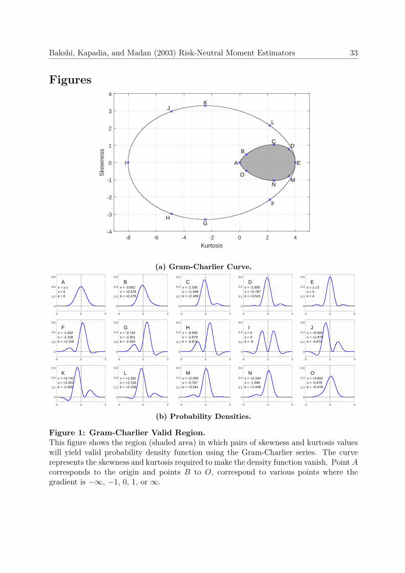
Figure 1: Gram-Charlier Valid Region.This figure shows the region (shaded area) in which pairs of skewness and kurtosis valueswill yield valid probability density function using the Gram-Charlier series. The curverepresents the skewness and kurtosis required to make the density function vanish. Point Acorresponds to the origin and points B to O, correspond to various points where thegradient is −∞, −1, 0, 1, or ∞.
Bakshi, Kapadia, and Madan (2003) Risk-Neutral Moment Estimators 34
0 0.5 1 1.5 2 2.5 3 3.5 4 4.5
Kurtosis
-1.5
-1
-0.5
0
0.5
1
1.5
Ske
wne
ss
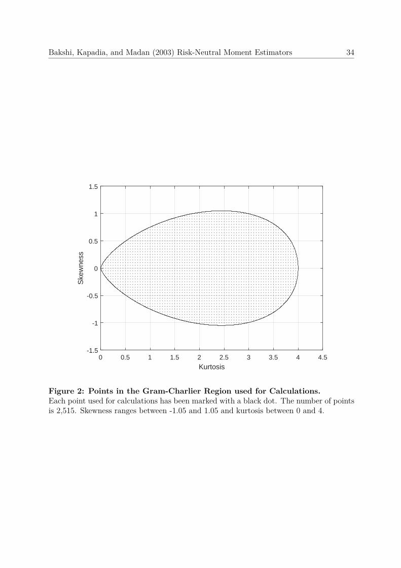
Figure 2: Points in the Gram-Charlier Region used for Calculations.Each point used for calculations has been marked with a black dot. The number of pointsis 2,515. Skewness ranges between -1.05 and 1.05 and kurtosis between 0 and 4.

Bakshi, Kapadia, and Madan (2003) Risk-Neutral Moment Estimators 35
0 0.5 1 1.5 2 2.5 3 3.5 4Kurtosis
-1.5
-1
-0.5
0
0.5
1
1.5S
kew
ness
-4
-3
-2
-1
0
1
2
3
4
Err
or =
Est
imat
ed -
Tru
e
10-4
(a) Skewness Error
0 0.5 1 1.5 2 2.5 3 3.5 4Kurtosis
-1.5
-1
-0.5
0
0.5
1
1.5
Ske
wne
ss
2
2.5
3
3.5
4
Err
or =
Est
imat
ed -
Tru
e
10-3
(b) Kurtosis Error
Figure 3: Example of the Errors for Skewness and Kurtosis.These figures show the errors between the estimated skewness (a) and kurtosis (b) (usingthe BKM method) and their true values. Based on the valid Gram-Charlier region, ofwhich 2,515 pairs of true skewness and kurtosis values were used to calculated the errorsurface. For this set of figures, K ∈ [500, 8000] (a = 0.25) and ∆K = 1.
Bakshi, Kapadia, and Madan (2003) Risk-Neutral Moment Estimators 36
0 10 20 30 40 50
K
0
0.1
0.2
0.3
0.4
0.5
0.6
0.7
0.8
0.9
1
Wid
th (
a [F
0a,
F0/a
])
-0.3
-0.2
-0.1
0
0.1
0.2
0.3
Err
or =
Est
imat
ed -
Tru
e
-0.41
10
-0.3
20
K
Width (a [F0
a, F0/a])
0.5
-0.2
30
Ave
rage
Ske
wne
ss E
rror
40
-0.1
050
0
-0.3
-0.2
-0.1
0
0.1
0.2
0.3
Err
or =
Est
imat
ed -
Tru
e
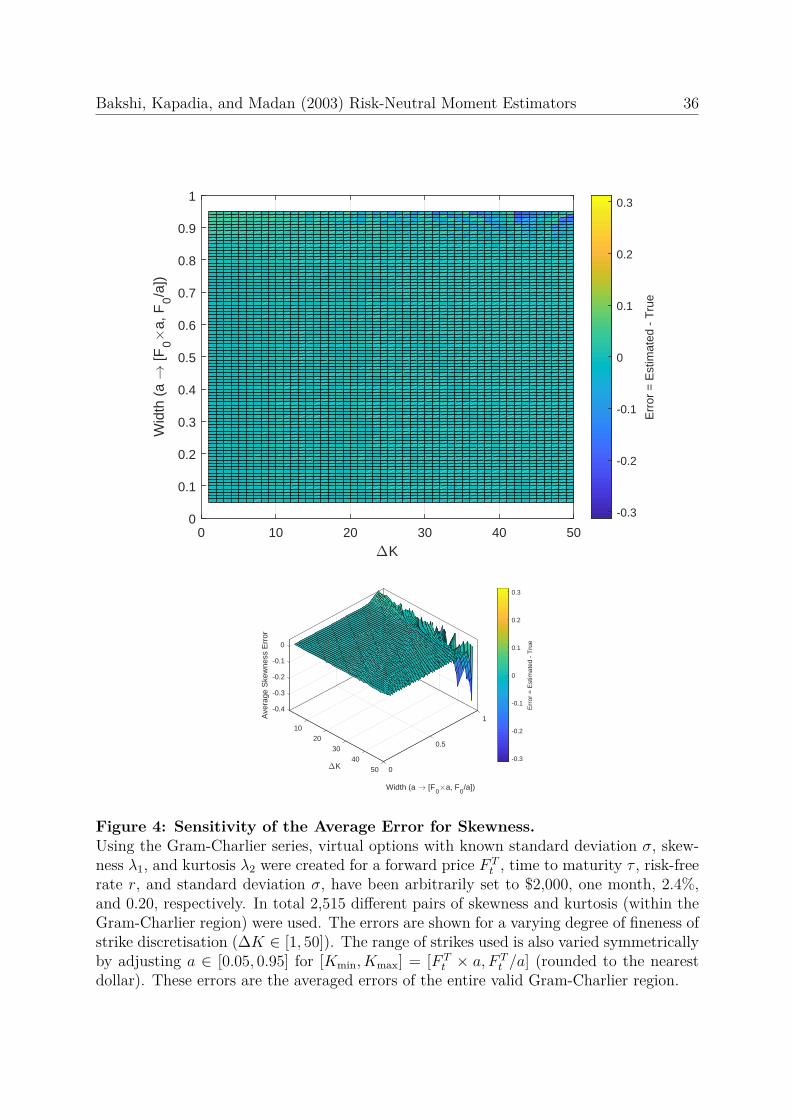
Figure 4: Sensitivity of the Average Error for Skewness.Using the Gram-Charlier series, virtual options with known standard deviation σ, skew-ness λ1, and kurtosis λ2 were created for a forward price F T
t , time to maturity τ , risk-freerate r, and standard deviation σ, have been arbitrarily set to $2,000, one month, 2.4%,and 0.20, respectively. In total 2,515 different pairs of skewness and kurtosis (within theGram-Charlier region) were used. The errors are shown for a varying degree of fineness ofstrike discretisation (∆K ∈ [1, 50]). The range of strikes used is also varied symmetricallyby adjusting a ∈ [0.05, 0.95] for [Kmin, Kmax] = [F T
t × a, F Tt /a] (rounded to the nearest
dollar). These errors are the averaged errors of the entire valid Gram-Charlier region.

Bakshi, Kapadia, and Madan (2003) Risk-Neutral Moment Estimators 37
0 5 10 15 20 25 30 35 40 45 50
K
-8
-6
-4
-2
0
2
4
6
8
Ave
rage
Ske
wne
ss E
rror
10-3
a = 0.05a = 0.40a = 0.75
0 5 10 15 20 25
K
-1
-0.5
0
0.5
1
1.5
Ave
rage
Ske
wne
ss E
rror
10-3
a = 0.05a = 0.40a = 0.75
0 1 2 3 4 5 6 7 8 9 10
K
-1
-0.8
-0.6
-0.4
-0.2
0
0.2
0.4
0.6
0.8
1
Ave
rage
Ske
wne
ss E
rror
10-3
a = 0.05a = 0.40a = 0.75
(a) Mean Skewness Error.
0 5 10 15 20 25 30 35 40 45 50
K
0
0.005
0.01
0.015
0.02
0.025
0.03
0.035
0.04
0.045
0.05
Max
imum
Abs
olut
e S
kew
ness
Err
or
a = 0.05a = 0.40a = 0.75
0 5 10 15 20 25
K
0
0.005
0.01
0.015
Max
imum
Abs
olut
e S
kew
ness
Err
or
a = 0.05a = 0.40a = 0.75
0 1 2 3 4 5 6 7 8 9 10
K
0
0.5
1
1.5
2
2.5
3
3.5
4
Max
imum
Abs
olut
e S
kew
ness
Err
or
10-3
a = 0.05a = 0.40a = 0.75
(b) Maximum Absolute Skewness Error.
0 5 10 15 20 25 30 35 40 45 50
K
-0.3
-0.25
-0.2
-0.15
-0.1
-0.05
0
0.05
0.1
0.15
0.2
Ave
rage
Kur
tosi
s E
rror
a = 0.05a = 0.40a = 0.75
0 5 10 15 20 25
K
-0.1
-0.05
0
0.05
Ave
rage
Kur
tosi
s E
rror
a = 0.05a = 0.40a = 0.75
0 1 2 3 4 5 6 7 8 9 10
K
-0.03
-0.025
-0.02
-0.015
-0.01
-0.005
0
0.005
0.01
0.015
0.02
Ave
rage
Kur
tosi
s E
rror
a = 0.05a = 0.40a = 0.75
(c) Mean Kurtosis Error.
0 5 10 15 20 25 30 35 40 45 50
K
0
0.05
0.1
0.15
0.2
0.25
0.3
0.35
0.4
0.45
Max
imum
Abs
olut
e K
urto
sis
Err
or
a = 0.05a = 0.40a = 0.75
0 5 10 15 20 25
K
0
0.02
0.04
0.06
0.08
0.1
0.12
0.14
Max
imum
Abs
olut
e K
urto
sis
Err
or
a = 0.05a = 0.40a = 0.75
0 1 2 3 4 5 6 7 8 9 10
K
0
0.005
0.01
0.015
0.02
0.025
0.03
0.035
0.04
Max
imum
Abs
olut
e K
urto
sis
Err
or
a = 0.05a = 0.40a = 0.75
(d) Maximum Absolute Kurtosis Error.
Figure 5: Errors w.r.t. ∆K.These figures have been created for boundary controlling factor values of 0.05, 0.40, and0.75 and for step sizes of ∆K from 1 to 50, to 25, and to 10. The error boundary of 10−3
is shown in red.

Bakshi, Kapadia, and Madan (2003) Risk-Neutral Moment Estimators 38
0 0.1 0.2 0.3 0.4 0.5 0.6 0.7 0.8 0.9 1
Boundary Controlling Factor (a)
-0.1
-0.05
0
0.05
Ave
rage
Ske
wne
ss E
rror
K = 1 K = 10 K = 25
0 0.1 0.2 0.3 0.4 0.5 0.6 0.7
Boundary Controlling Factor (a)
-1.5
-1
-0.5
0
0.5
1
1.5
Ave
rage
Ske
wne
ss E
rror
10-3
K = 1 K = 10 K = 25
0 0.05 0.1 0.15 0.2 0.25 0.3 0.35 0.4 0.45 0.5
Boundary Controlling Factor (a)
-1.5
-1
-0.5
0
0.5
1
1.5
Ave
rage
Ske
wne
ss E
rror
10-3
K = 1 K = 10 K = 25
(a) Mean Skewness Error.
0 0.1 0.2 0.3 0.4 0.5 0.6 0.7 0.8 0.9 1
Boundary Controlling Factor (a)
0
0.1
0.2
0.3
0.4
0.5
0.6
0.7
0.8
0.9
Max
imum
Abs
olut
e S
kew
ness
Err
or
K = 1 K = 10 K = 25
0 0.1 0.2 0.3 0.4 0.5 0.6 0.7
Boundary Controlling Factor (a)
0
0.002
0.004
0.006
0.008
0.01
0.012
Max
imum
Abs
olut
e S
kew
ness
Err
or
K = 1 K = 10 K = 25
0 0.05 0.1 0.15 0.2 0.25 0.3 0.35 0.4 0.45 0.5
Boundary Controlling Factor (a)
0
0.002
0.004
0.006
0.008
0.01
0.012
Max
imum
Abs
olut
e S
kew
ness
Err
or
K = 1 K = 10 K = 25
(b) Maximum Absolute Skewness Error.
0 0.1 0.2 0.3 0.4 0.5 0.6 0.7 0.8 0.9 1
Boundary Controlling Factor (a)
-4
-3.5
-3
-2.5
-2
-1.5
-1
-0.5
0
0.5
Ave
rage
Kur
tosi
s E
rror
K = 1 K = 10 K = 25
0 0.1 0.2 0.3 0.4 0.5 0.6 0.7
Boundary Controlling Factor (a)
-0.08
-0.06
-0.04
-0.02
0
0.02
0.04
0.06
Ave
rage
Kur
tosi
s E
rror
K = 1 K = 10 K = 25
0 0.05 0.1 0.15 0.2 0.25 0.3 0.35 0.4 0.45 0.5
Boundary Controlling Factor (a)
-0.08
-0.06
-0.04
-0.02
0
0.02
0.04
0.06
Ave
rage
Kur
tosi
s E
rror
K = 1 K = 10 K = 25
(c) Mean Kurtosis Error.
0 0.1 0.2 0.3 0.4 0.5 0.6 0.7 0.8 0.9 1
Boundary Controlling Factor (a)
0
1
2
3
4
5
6
Max
imum
Abs
olut
e K
urto
sis
Err
or
K = 1 K = 10 K = 25
0 0.1 0.2 0.3 0.4 0.5 0.6 0.7
Boundary Controlling Factor (a)
0
0.01
0.02
0.03
0.04
0.05
0.06
0.07
0.08
0.09
0.1
Max
imum
Abs
olut
e K
urto
sis
Err
or
K = 1 K = 10 K = 25
0 0.05 0.1 0.15 0.2 0.25 0.3 0.35 0.4 0.45 0.5
Boundary Controlling Factor (a)
0
0.01
0.02
0.03
0.04
0.05
0.06
0.07
0.08
0.09
0.1
Max
imum
Abs
olut
e K
urto
sis
Err
or
K = 1 K = 10 K = 25
(d) Maximum Absolute Kurtosis Error.
Figure 6: Errors w.r.t. a.These figures have been created for step sizes of 1, 10, and 25 and for boundary controllingfactors of a from 0.05 to 0.95, to 0.75, and to 0.50. The error boundary of 10−3 is shownin red.
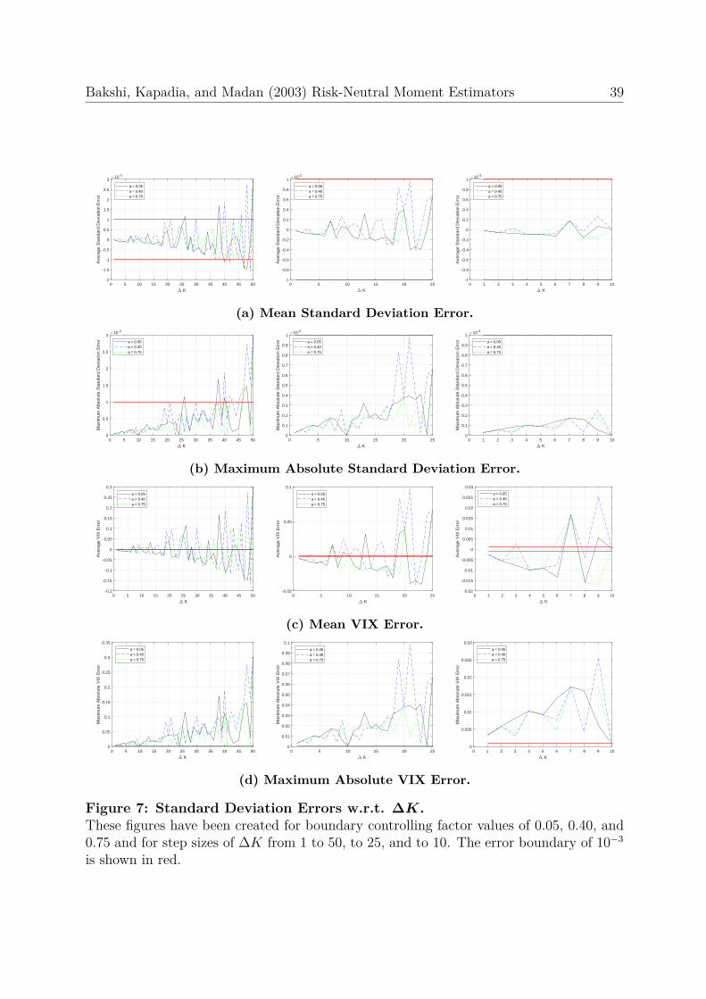
Bakshi, Kapadia, and Madan (2003) Risk-Neutral Moment Estimators 39
0 5 10 15 20 25 30 35 40 45 50
K
-2
-1.5
-1
-0.5
0
0.5
1
1.5
2
2.5
3
Ave
rage
Sta
ndar
d D
evia
tion
Err
or
10-3
a = 0.05a = 0.40a = 0.75
0 5 10 15 20 25
K
-1
-0.8
-0.6
-0.4
-0.2
0
0.2
0.4
0.6
0.8
1
Ave
rage
Sta
ndar
d D
evia
tion
Err
or
10-3
a = 0.05a = 0.40a = 0.75
0 1 2 3 4 5 6 7 8 9 10
K
-1
-0.8
-0.6
-0.4
-0.2
0
0.2
0.4
0.6
0.8
1
Ave
rage
Sta
ndar
d D
evia
tion
Err
or
10-3
a = 0.05a = 0.40a = 0.75
(a) Mean Standard Deviation Error.
0 5 10 15 20 25 30 35 40 45 50
K
0
0.5
1
1.5
2
2.5
3
Max
imum
Abs
olut
e S
tand
ard
Dev
iatio
n E
rror
10-3
a = 0.05a = 0.40a = 0.75
0 5 10 15 20 25
K
0
0.1
0.2
0.3
0.4
0.5
0.6
0.7
0.8
0.9
1
Max
imum
Abs
olut
e S
tand
ard
Dev
iatio
n E
rror
10-3
a = 0.05a = 0.40a = 0.75
0 1 2 3 4 5 6 7 8 9 10
K
0
0.1
0.2
0.3
0.4
0.5
0.6
0.7
0.8
0.9
1
Max
imum
Abs
olut
e S
tand
ard
Dev
iatio
n E
rror
10-3
a = 0.05a = 0.40a = 0.75
(b) Maximum Absolute Standard Deviation Error.
0 5 10 15 20 25 30 35 40 45 50
K
-0.2
-0.15
-0.1
-0.05
0
0.05
0.1
0.15
0.2
0.25
0.3
Ave
rage
VIX
Err
or
a = 0.05a = 0.40a = 0.75
0 5 10 15 20 25
K
-0.05
0
0.05
0.1
Ave
rage
VIX
Err
or
a = 0.05a = 0.40a = 0.75
0 1 2 3 4 5 6 7 8 9 10
K
-0.02
-0.015
-0.01
-0.005
0
0.005
0.01
0.015
0.02
0.025
0.03
Ave
rage
VIX
Err
or
a = 0.05a = 0.40a = 0.75
(c) Mean VIX Error.
0 5 10 15 20 25 30 35 40 45 50
K
0
0.05
0.1
0.15
0.2
0.25
0.3
0.35
Max
imum
Abs
olut
e V
IX E
rror
a = 0.05a = 0.40a = 0.75
0 5 10 15 20 25
K
0
0.01
0.02
0.03
0.04
0.05
0.06
0.07
0.08
0.09
0.1
Max
imum
Abs
olut
e V
IX E
rror
a = 0.05a = 0.40a = 0.75
0 1 2 3 4 5 6 7 8 9 10
K
0
0.005
0.01
0.015
0.02
0.025
0.03
Max
imum
Abs
olut
e V
IX E
rror
a = 0.05a = 0.40a = 0.75
(d) Maximum Absolute VIX Error.
Figure 7: Standard Deviation Errors w.r.t. ∆K.These figures have been created for boundary controlling factor values of 0.05, 0.40, and0.75 and for step sizes of ∆K from 1 to 50, to 25, and to 10. The error boundary of 10−3
is shown in red.
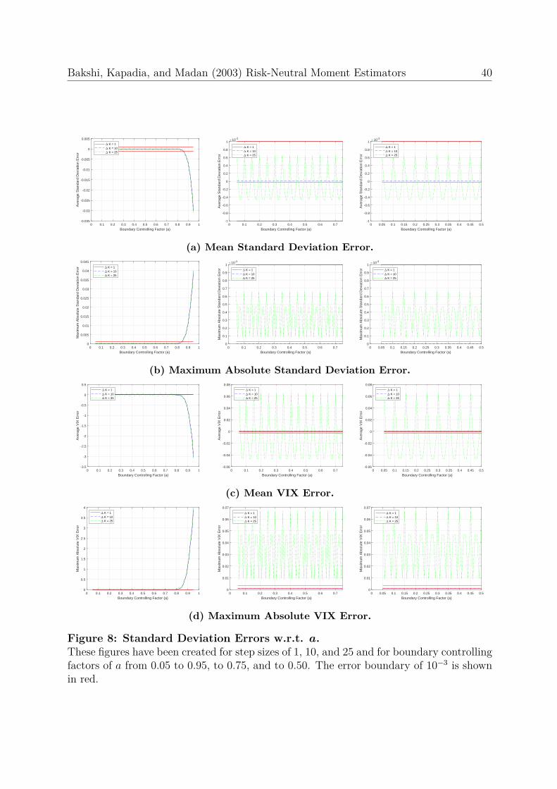
Bakshi, Kapadia, and Madan (2003) Risk-Neutral Moment Estimators 40
0 0.1 0.2 0.3 0.4 0.5 0.6 0.7 0.8 0.9 1
Boundary Controlling Factor (a)
-0.035
-0.03
-0.025
-0.02
-0.015
-0.01
-0.005
0
0.005
Ave
rage
Sta
ndar
d D
evia
tion
Err
or
K = 1 K = 10 K = 25
0 0.1 0.2 0.3 0.4 0.5 0.6 0.7
Boundary Controlling Factor (a)
-1
-0.8
-0.6
-0.4
-0.2
0
0.2
0.4
0.6
0.8
1
Ave
rage
Sta
ndar
d D
evia
tion
Err
or
10-3
K = 1 K = 10 K = 25
0 0.05 0.1 0.15 0.2 0.25 0.3 0.35 0.4 0.45 0.5
Boundary Controlling Factor (a)
-1
-0.8
-0.6
-0.4
-0.2
0
0.2
0.4
0.6
0.8
1
Ave
rage
Sta
ndar
d D
evia
tion
Err
or
10-3
K = 1 K = 10 K = 25
(a) Mean Standard Deviation Error.
0 0.1 0.2 0.3 0.4 0.5 0.6 0.7 0.8 0.9 1
Boundary Controlling Factor (a)
0
0.005
0.01
0.015
0.02
0.025
0.03
0.035
0.04
0.045
Max
imum
Abs
olut
e S
tand
ard
Dev
iatio
n E
rror K = 1
K = 10 K = 25
0 0.1 0.2 0.3 0.4 0.5 0.6 0.7
Boundary Controlling Factor (a)
0
0.1
0.2
0.3
0.4
0.5
0.6
0.7
0.8
0.9
1
Max
imum
Abs
olut
e S
tand
ard
Dev
iatio
n E
rror
10-3
K = 1 K = 10 K = 25
0 0.05 0.1 0.15 0.2 0.25 0.3 0.35 0.4 0.45 0.5
Boundary Controlling Factor (a)
0
0.1
0.2
0.3
0.4
0.5
0.6
0.7
0.8
0.9
1
Max
imum
Abs
olut
e S
tand
ard
Dev
iatio
n E
rror
10-3
K = 1 K = 10 K = 25
(b) Maximum Absolute Standard Deviation Error.
0 0.1 0.2 0.3 0.4 0.5 0.6 0.7 0.8 0.9 1
Boundary Controlling Factor (a)
-3.5
-3
-2.5
-2
-1.5
-1
-0.5
0
0.5
Ave
rage
VIX
Err
or
K = 1 K = 10 K = 25
0 0.1 0.2 0.3 0.4 0.5 0.6 0.7
Boundary Controlling Factor (a)
-0.06
-0.04
-0.02
0
0.02
0.04
0.06
0.08
Ave
rage
VIX
Err
or
K = 1 K = 10 K = 25
0 0.05 0.1 0.15 0.2 0.25 0.3 0.35 0.4 0.45 0.5
Boundary Controlling Factor (a)
-0.06
-0.04
-0.02
0
0.02
0.04
0.06
0.08
Ave
rage
VIX
Err
or
K = 1 K = 10 K = 25
(c) Mean VIX Error.
0 0.1 0.2 0.3 0.4 0.5 0.6 0.7 0.8 0.9 1
Boundary Controlling Factor (a)
0
0.5
1
1.5
2
2.5
3
3.5
4
Max
imum
Abs
olut
e V
IX E
rror
K = 1 K = 10 K = 25
0 0.1 0.2 0.3 0.4 0.5 0.6 0.7
Boundary Controlling Factor (a)
0
0.01
0.02
0.03
0.04
0.05
0.06
0.07
Max
imum
Abs
olut
e V
IX E
rror
K = 1 K = 10 K = 25
0 0.05 0.1 0.15 0.2 0.25 0.3 0.35 0.4 0.45 0.5
Boundary Controlling Factor (a)
0
0.01
0.02
0.03
0.04
0.05
0.06
0.07
Max
imum
Abs
olut
e V
IX E
rror
K = 1 K = 10 K = 25
(d) Maximum Absolute VIX Error.
Figure 8: Standard Deviation Errors w.r.t. a.These figures have been created for step sizes of 1, 10, and 25 and for boundary controllingfactors of a from 0.05 to 0.95, to 0.75, and to 0.50. The error boundary of 10−3 is shownin red.
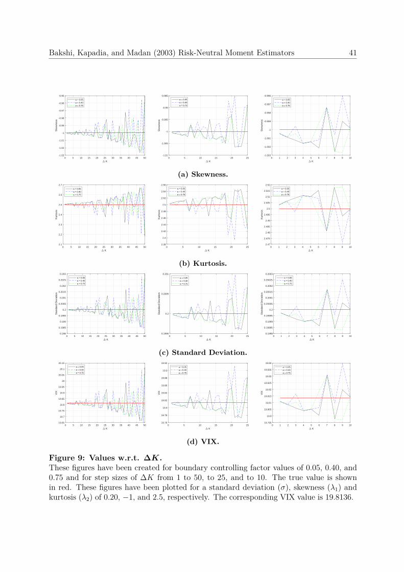
Bakshi, Kapadia, and Madan (2003) Risk-Neutral Moment Estimators 41
0 5 10 15 20 25 30 35 40 45 50
K
-1.03
-1.02
-1.01
-1
-0.99
-0.98
-0.97
-0.96
-0.95
Ske
wne
ss
a = 0.05a = 0.40a = 0.75
0 5 10 15 20 25
K
-1.01
-1.005
-1
-0.995
-0.99
-0.985
Ske
wne
ss
a = 0.05a = 0.40a = 0.75
0 1 2 3 4 5 6 7 8 9 10
K
-1.003
-1.002
-1.001
-1
-0.999
-0.998
-0.997
-0.996
Ske
wne
ss
a = 0.05a = 0.40a = 0.75
(a) Skewness.
0 5 10 15 20 25 30 35 40 45 50
K
2.1
2.2
2.3
2.4
2.5
2.6
2.7
Kur
tosi
s
a = 0.05a = 0.40a = 0.75
0 5 10 15 20 25
K
2.38
2.4
2.42
2.44
2.46
2.48
2.5
2.52
2.54
2.56
Kur
tosi
s
a = 0.05a = 0.40a = 0.75
0 1 2 3 4 5 6 7 8 9 10
K
2.47
2.475
2.48
2.485
2.49
2.495
2.5
2.505
2.51
2.515
2.52
Kur
tosi
s
a = 0.05a = 0.40a = 0.75
(b) Kurtosis.
0 5 10 15 20 25 30 35 40 45 50
K
0.198
0.1985
0.199
0.1995
0.2
0.2005
0.201
0.2015
0.202
0.2025
0.203
Sta
ndar
d D
evia
tion
a = 0.05a = 0.40a = 0.75
0 5 10 15 20 25
K
0.1995
0.2
0.2005
0.201
Sta
ndar
d D
evia
tion
a = 0.05a = 0.40a = 0.75
0 1 2 3 4 5 6 7 8 9 10
K
0.1998
0.19985
0.1999
0.19995
0.2
0.20005
0.2001
0.20015
0.2002
0.20025
0.2003
Sta
ndar
d D
evia
tion
a = 0.05a = 0.40a = 0.75
(c) Standard Deviation.
0 5 10 15 20 25 30 35 40 45 50
K
19.65
19.7
19.75
19.8
19.85
19.9
19.95
20
20.05
20.1
20.15
VIX
a = 0.05a = 0.40a = 0.75
0 5 10 15 20 25
K
19.76
19.78
19.8
19.82
19.84
19.86
19.88
19.9
19.92
VIX
a = 0.05a = 0.40a = 0.75
0 1 2 3 4 5 6 7 8 9 10
K
19.795
19.8
19.805
19.81
19.815
19.82
19.825
19.83
19.835
19.84
VIX
a = 0.05a = 0.40a = 0.75
(d) VIX.
Figure 9: Values w.r.t. ∆K.These figures have been created for boundary controlling factor values of 0.05, 0.40, and0.75 and for step sizes of ∆K from 1 to 50, to 25, and to 10. The true value is shownin red. These figures have been plotted for a standard deviation (σ), skewness (λ1) andkurtosis (λ2) of 0.20, −1, and 2.5, respectively. The corresponding VIX value is 19.8136.
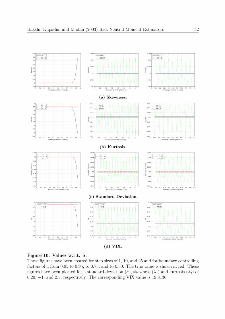
Bakshi, Kapadia, and Madan (2003) Risk-Neutral Moment Estimators 42
0 0.1 0.2 0.3 0.4 0.5 0.6 0.7 0.8 0.9 1
Boundary Controlling Factor (a)
-1.1
-1
-0.9
-0.8
-0.7
-0.6
-0.5
-0.4
-0.3
-0.2
Ske
wne
ss
K = 1 K = 10 K = 25
0 0.1 0.2 0.3 0.4 0.5 0.6 0.7
Boundary Controlling Factor (a)
-1.01
-1.005
-1
-0.995
-0.99
-0.985
Ske
wne
ss
K = 1 K = 10 K = 25
0 0.05 0.1 0.15 0.2 0.25 0.3 0.35 0.4 0.45 0.5
Boundary Controlling Factor (a)
-1.01
-1.005
-1
-0.995
-0.99
-0.985
Ske
wne
ss
K = 1 K = 10 K = 25
(a) Skewness.
0 0.1 0.2 0.3 0.4 0.5 0.6 0.7 0.8 0.9 1
Boundary Controlling Factor (a)
-1.5
-1
-0.5
0
0.5
1
1.5
2
2.5
3
Kur
tosi
s
K = 1 K = 10 K = 25
0 0.1 0.2 0.3 0.4 0.5 0.6 0.7
Boundary Controlling Factor (a)
2.42
2.44
2.46
2.48
2.5
2.52
2.54
2.56
Kur
tosi
s
K = 1 K = 10 K = 25
0 0.05 0.1 0.15 0.2 0.25 0.3 0.35 0.4 0.45 0.5
Boundary Controlling Factor (a)
2.42
2.44
2.46
2.48
2.5
2.52
2.54
2.56
Kur
tosi
s
K = 1 K = 10 K = 25
(b) Kurtosis.
0 0.1 0.2 0.3 0.4 0.5 0.6 0.7 0.8 0.9 1
Boundary Controlling Factor (a)
0.165
0.17
0.175
0.18
0.185
0.19
0.195
0.2
0.205
Sta
ndar
d D
evia
tion
K = 1 K = 10 K = 25
0 0.1 0.2 0.3 0.4 0.5 0.6 0.7
Boundary Controlling Factor (a)
0.1994
0.1996
0.1998
0.2
0.2002
0.2004
0.2006
0.2008
Sta
ndar
d D
evia
tion
K = 1 K = 10 K = 25
0 0.05 0.1 0.15 0.2 0.25 0.3 0.35 0.4 0.45 0.5
Boundary Controlling Factor (a)
0.1994
0.1996
0.1998
0.2
0.2002
0.2004
0.2006
0.2008
Sta
ndar
d D
evia
tion
K = 1 K = 10 K = 25
(c) Standard Deviation.
0 0.1 0.2 0.3 0.4 0.5 0.6 0.7 0.8 0.9 1
Boundary Controlling Factor (a)
16.5
17
17.5
18
18.5
19
19.5
20
VIX
K = 1 K = 10 K = 25
0 0.1 0.2 0.3 0.4 0.5 0.6 0.7
Boundary Controlling Factor (a)
19.76
19.78
19.8
19.82
19.84
19.86
19.88
19.9
VIX
K = 1 K = 10 K = 25
0 0.05 0.1 0.15 0.2 0.25 0.3 0.35 0.4 0.45 0.5
Boundary Controlling Factor (a)
19.76
19.78
19.8
19.82
19.84
19.86
19.88
19.9
VIX
K = 1 K = 10 K = 25
(d) VIX.
Figure 10: Values w.r.t. a.These figures have been created for step sizes of 1, 10, and 25 and for boundary controllingfactors of a from 0.05 to 0.95, to 0.75, and to 0.50. The true value is shown in red. Thesefigures have been plotted for a standard deviation (σ), skewness (λ1) and kurtosis (λ2) of0.20, −1, and 2.5, respectively. The corresponding VIX value is 19.8136.
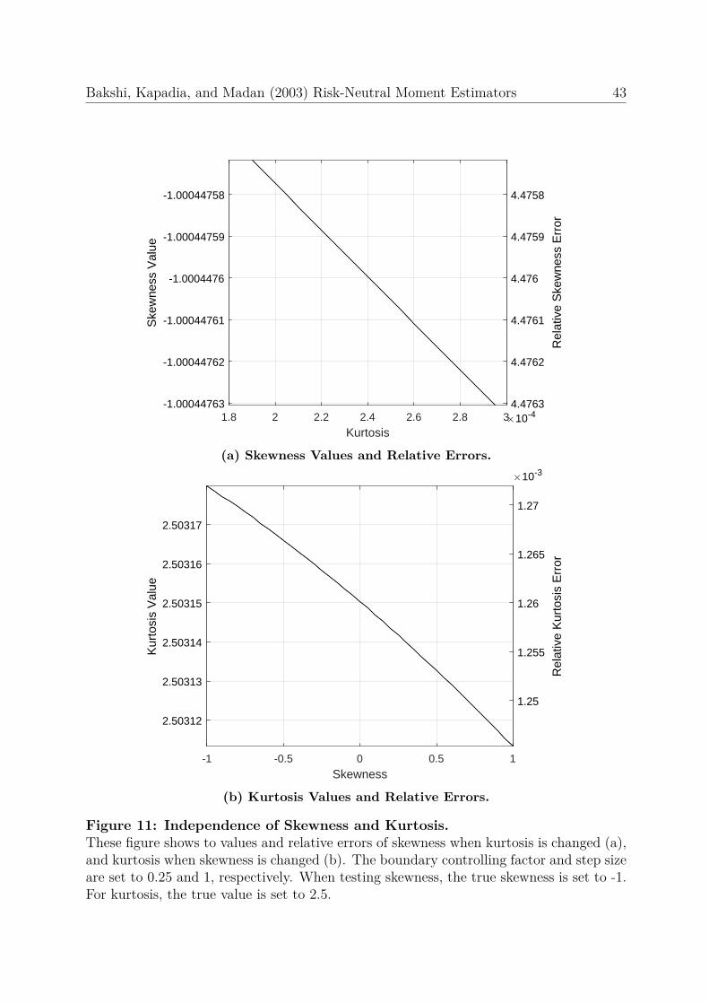
Bakshi, Kapadia, and Madan (2003) Risk-Neutral Moment Estimators 43
1.8 2 2.2 2.4 2.6 2.8 3
Kurtosis
-1.00044763
-1.00044762
-1.00044761
-1.0004476
-1.00044759
-1.00044758
Ske
wne
ss V
alue
4.4758
4.4759
4.476
4.4761
4.4762
4.4763
Rel
ativ
e S
kew
ness
Err
or
10-4
(a) Skewness Values and Relative Errors.
-1 -0.5 0 0.5 1
Skewness
2.50312
2.50313
2.50314
2.50315
2.50316
2.50317
Kur
tosi
s V
alue
1.25
1.255
1.26
1.265
1.27
Rel
ativ
e K
urto
sis
Err
or
10-3
(b) Kurtosis Values and Relative Errors.
Figure 11: Independence of Skewness and Kurtosis.These figure shows to values and relative errors of skewness when kurtosis is changed (a),and kurtosis when skewness is changed (b). The boundary controlling factor and step sizeare set to 0.25 and 1, respectively. When testing skewness, the true skewness is set to -1.For kurtosis, the true value is set to 2.5.
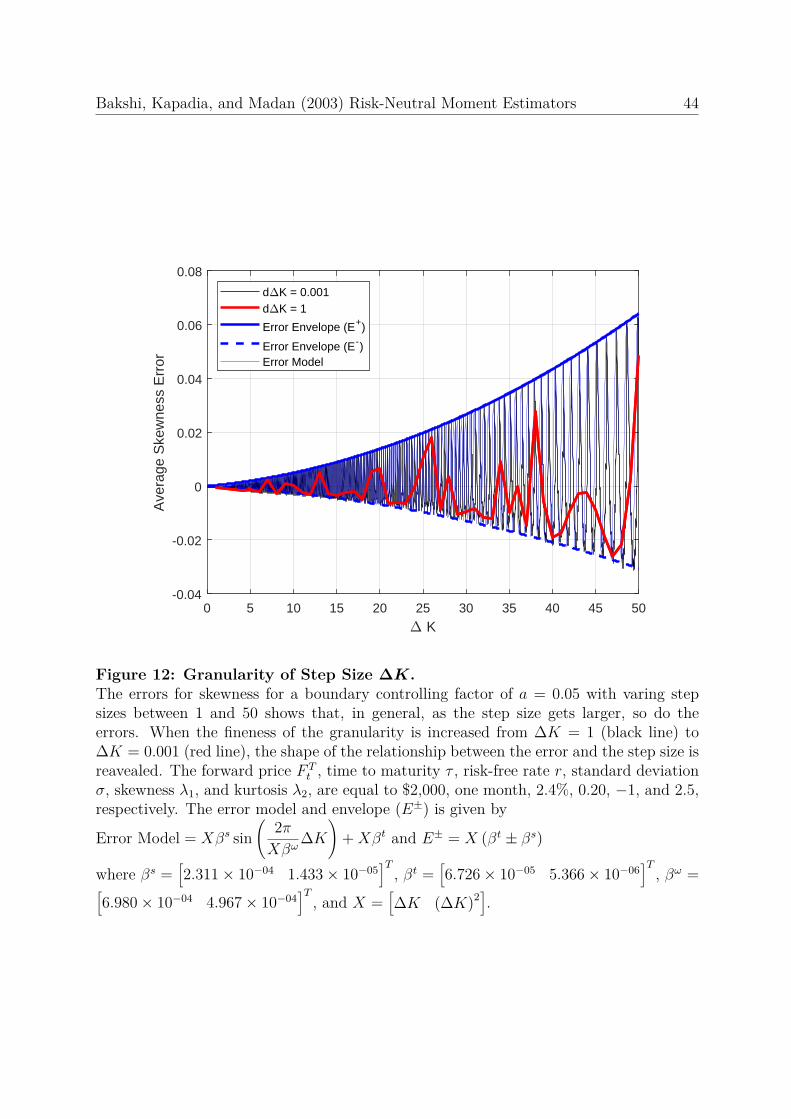
Bakshi, Kapadia, and Madan (2003) Risk-Neutral Moment Estimators 44
0 5 10 15 20 25 30 35 40 45 50
K
-0.04
-0.02
0
0.02
0.04
0.06
0.08
Ave
rage
Ske
wne
ss E
rror
d K = 0.001d K = 1
Error Envelope (E+)
Error Envelope (E-)Error Model
Figure 12: Granularity of Step Size ∆K.The errors for skewness for a boundary controlling factor of a = 0.05 with varing stepsizes between 1 and 50 shows that, in general, as the step size gets larger, so do theerrors. When the fineness of the granularity is increased from ∆K = 1 (black line) to∆K = 0.001 (red line), the shape of the relationship between the error and the step size isreavealed. The forward price F T
t , time to maturity τ , risk-free rate r, standard deviationσ, skewness λ1, and kurtosis λ2, are equal to $2,000, one month, 2.4%, 0.20, −1, and 2.5,respectively. The error model and envelope (E±) is given by
Error Model = Xβs sin(
2πXβω
∆K)
+Xβt and E± = X (βt ± βs)
where βs =[2.311× 10−04 1.433× 10−05
]T, βt =
[6.726× 10−05 5.366× 10−06
]T, βω =[
6.980× 10−04 4.967× 10−04]T, and X =
[∆K (∆K)2
].
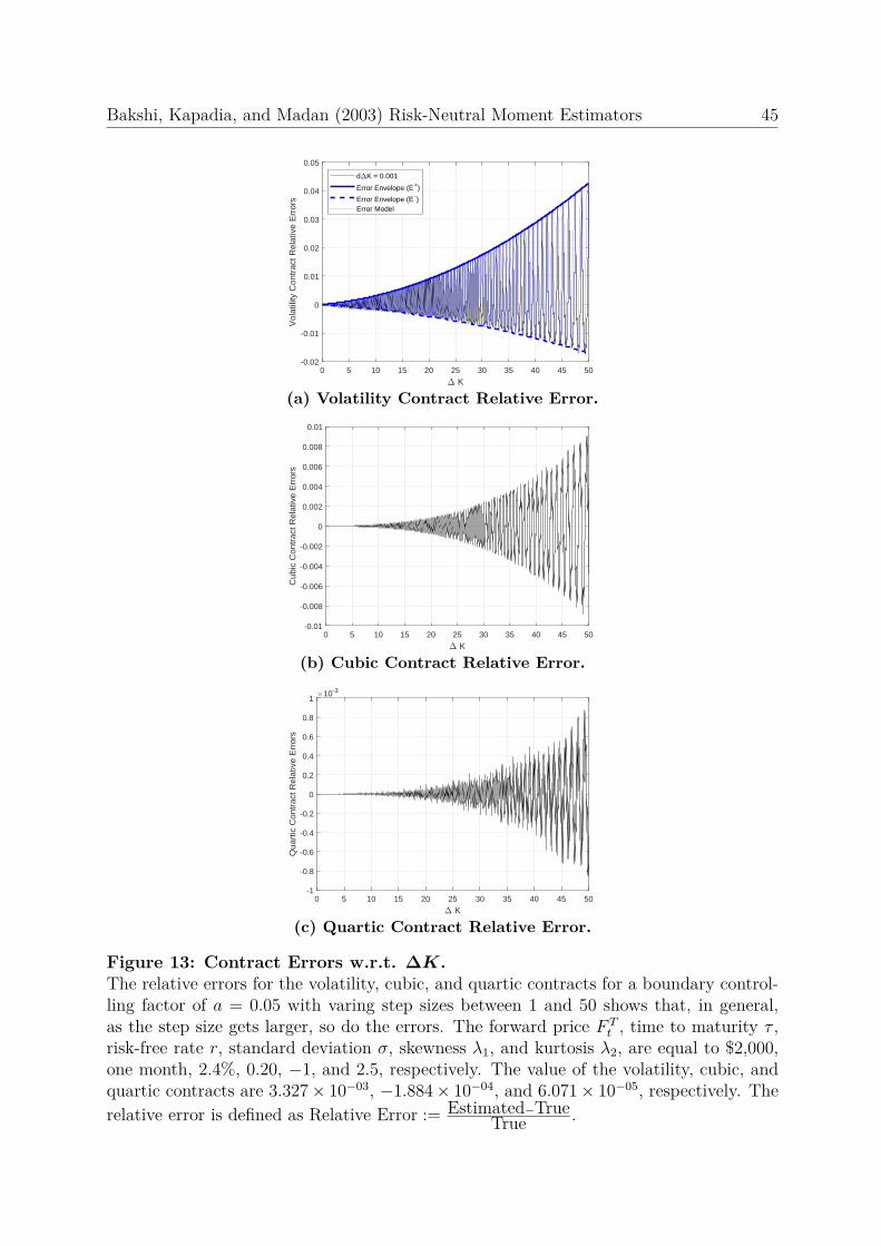
Bakshi, Kapadia, and Madan (2003) Risk-Neutral Moment Estimators 45
0 5 10 15 20 25 30 35 40 45 50
K
-0.02
-0.01
0
0.01
0.02
0.03
0.04
0.05
Vol
atili
ty C
ontr
act R
elat
ive
Err
ors
d K = 0.001
Error Envelope (E+)
Error Envelope (E-)Error Model
(a) Volatility Contract Relative Error.
0 5 10 15 20 25 30 35 40 45 50
K
-0.01
-0.008
-0.006
-0.004
-0.002
0
0.002
0.004
0.006
0.008
0.01
Cub
ic C
ontr
act R
elat
ive
Err
ors
(b) Cubic Contract Relative Error.
0 5 10 15 20 25 30 35 40 45 50
K
-1
-0.8
-0.6
-0.4
-0.2
0
0.2
0.4
0.6
0.8
1
Qua
rtic
Con
trac
t Rel
ativ
e E
rror
s
10-3
(c) Quartic Contract Relative Error.
Figure 13: Contract Errors w.r.t. ∆K.The relative errors for the volatility, cubic, and quartic contracts for a boundary control-ling factor of a = 0.05 with varing step sizes between 1 and 50 shows that, in general,as the step size gets larger, so do the errors. The forward price F T
t , time to maturity τ ,risk-free rate r, standard deviation σ, skewness λ1, and kurtosis λ2, are equal to $2,000,one month, 2.4%, 0.20, −1, and 2.5, respectively. The value of the volatility, cubic, andquartic contracts are 3.327× 10−03, −1.884× 10−04, and 6.071× 10−05, respectively. Therelative error is defined as Relative Error := Estimated−True
True .
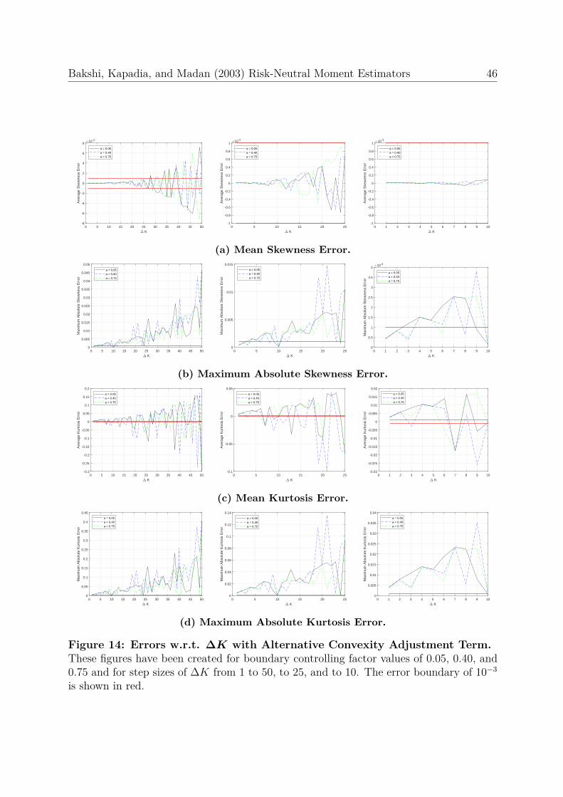
Bakshi, Kapadia, and Madan (2003) Risk-Neutral Moment Estimators 46
0 5 10 15 20 25 30 35 40 45 50
K
-8
-6
-4
-2
0
2
4
6
8
Ave
rage
Ske
wne
ss E
rror
10-3
a = 0.05a = 0.40a = 0.75
0 5 10 15 20 25
K
-1
-0.8
-0.6
-0.4
-0.2
0
0.2
0.4
0.6
0.8
1
Ave
rage
Ske
wne
ss E
rror
10-3
a = 0.05a = 0.40a = 0.75
0 1 2 3 4 5 6 7 8 9 10
K
-1
-0.8
-0.6
-0.4
-0.2
0
0.2
0.4
0.6
0.8
1
Ave
rage
Ske
wne
ss E
rror
10-3
a = 0.05a = 0.40a = 0.75
(a) Mean Skewness Error.
0 5 10 15 20 25 30 35 40 45 50
K
0
0.005
0.01
0.015
0.02
0.025
0.03
0.035
0.04
0.045
0.05
Max
imum
Abs
olut
e S
kew
ness
Err
or
a = 0.05a = 0.40a = 0.75
0 5 10 15 20 25
K
0
0.005
0.01
0.015
Max
imum
Abs
olut
e S
kew
ness
Err
or
a = 0.05a = 0.40a = 0.75
0 1 2 3 4 5 6 7 8 9 10
K
0
0.5
1
1.5
2
2.5
3
3.5
4
Max
imum
Abs
olut
e S
kew
ness
Err
or
10-3
a = 0.05a = 0.40a = 0.75
(b) Maximum Absolute Skewness Error.
0 5 10 15 20 25 30 35 40 45 50
K
-0.3
-0.25
-0.2
-0.15
-0.1
-0.05
0
0.05
0.1
0.15
0.2
Ave
rage
Kur
tosi
s E
rror
a = 0.05a = 0.40a = 0.75
0 5 10 15 20 25
K
-0.1
-0.05
0
0.05
Ave
rage
Kur
tosi
s E
rror
a = 0.05a = 0.40a = 0.75
0 1 2 3 4 5 6 7 8 9 10
K
-0.03
-0.025
-0.02
-0.015
-0.01
-0.005
0
0.005
0.01
0.015
0.02
Ave
rage
Kur
tosi
s E
rror
a = 0.05a = 0.40a = 0.75
(c) Mean Kurtosis Error.
0 5 10 15 20 25 30 35 40 45 50
K
0
0.05
0.1
0.15
0.2
0.25
0.3
0.35
0.4
0.45
Max
imum
Abs
olut
e K
urto
sis
Err
or
a = 0.05a = 0.40a = 0.75
0 5 10 15 20 25
K
0
0.02
0.04
0.06
0.08
0.1
0.12
0.14
Max
imum
Abs
olut
e K
urto
sis
Err
or
a = 0.05a = 0.40a = 0.75
0 1 2 3 4 5 6 7 8 9 10
K
0
0.005
0.01
0.015
0.02
0.025
0.03
0.035
0.04
Max
imum
Abs
olut
e K
urto
sis
Err
or
a = 0.05a = 0.40a = 0.75
(d) Maximum Absolute Kurtosis Error.
Figure 14: Errors w.r.t. ∆K with Alternative Convexity Adjustment Term.These figures have been created for boundary controlling factor values of 0.05, 0.40, and0.75 and for step sizes of ∆K from 1 to 50, to 25, and to 10. The error boundary of 10−3
is shown in red.
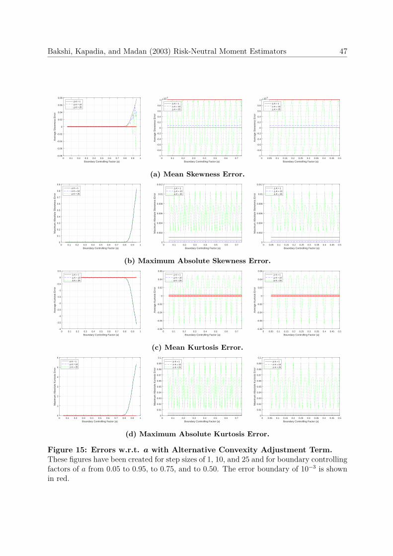
Bakshi, Kapadia, and Madan (2003) Risk-Neutral Moment Estimators 47
0 0.1 0.2 0.3 0.4 0.5 0.6 0.7 0.8 0.9 1
Boundary Controlling Factor (a)
-0.08
-0.06
-0.04
-0.02
0
0.02
0.04
0.06
0.08
Ave
rage
Ske
wne
ss E
rror
K = 1 K = 10 K = 25
0 0.1 0.2 0.3 0.4 0.5 0.6 0.7
Boundary Controlling Factor (a)
-1
-0.8
-0.6
-0.4
-0.2
0
0.2
0.4
0.6
0.8
1
Ave
rage
Ske
wne
ss E
rror
10-3
K = 1 K = 10 K = 25
0 0.05 0.1 0.15 0.2 0.25 0.3 0.35 0.4 0.45 0.5
Boundary Controlling Factor (a)
-1
-0.8
-0.6
-0.4
-0.2
0
0.2
0.4
0.6
0.8
1
Ave
rage
Ske
wne
ss E
rror
10-3
K = 1 K = 10 K = 25
(a) Mean Skewness Error.
0 0.1 0.2 0.3 0.4 0.5 0.6 0.7 0.8 0.9 1
Boundary Controlling Factor (a)
0
0.1
0.2
0.3
0.4
0.5
0.6
0.7
0.8
0.9
Max
imum
Abs
olut
e S
kew
ness
Err
or
K = 1 K = 10 K = 25
0 0.1 0.2 0.3 0.4 0.5 0.6 0.7
Boundary Controlling Factor (a)
0
0.002
0.004
0.006
0.008
0.01
0.012
Max
imum
Abs
olut
e S
kew
ness
Err
or
K = 1 K = 10 K = 25
0 0.05 0.1 0.15 0.2 0.25 0.3 0.35 0.4 0.45 0.5
Boundary Controlling Factor (a)
0
0.002
0.004
0.006
0.008
0.01
0.012
Max
imum
Abs
olut
e S
kew
ness
Err
or
K = 1 K = 10 K = 25
(b) Maximum Absolute Skewness Error.
0 0.1 0.2 0.3 0.4 0.5 0.6 0.7 0.8 0.9 1
Boundary Controlling Factor (a)
-4
-3.5
-3
-2.5
-2
-1.5
-1
-0.5
0
0.5
Ave
rage
Kur
tosi
s E
rror
K = 1 K = 10 K = 25
0 0.1 0.2 0.3 0.4 0.5 0.6 0.7
Boundary Controlling Factor (a)
-0.08
-0.06
-0.04
-0.02
0
0.02
0.04
0.06
Ave
rage
Kur
tosi
s E
rror
K = 1 K = 10 K = 25
0 0.05 0.1 0.15 0.2 0.25 0.3 0.35 0.4 0.45 0.5
Boundary Controlling Factor (a)
-0.08
-0.06
-0.04
-0.02
0
0.02
0.04
0.06
Ave
rage
Kur
tosi
s E
rror
K = 1 K = 10 K = 25
(c) Mean Kurtosis Error.
0 0.1 0.2 0.3 0.4 0.5 0.6 0.7 0.8 0.9 1
Boundary Controlling Factor (a)
0
1
2
3
4
5
6
Max
imum
Abs
olut
e K
urto
sis
Err
or
K = 1 K = 10 K = 25
0 0.1 0.2 0.3 0.4 0.5 0.6 0.7
Boundary Controlling Factor (a)
0
0.01
0.02
0.03
0.04
0.05
0.06
0.07
0.08
0.09
0.1
Max
imum
Abs
olut
e K
urto
sis
Err
or
K = 1 K = 10 K = 25
0 0.05 0.1 0.15 0.2 0.25 0.3 0.35 0.4 0.45 0.5
Boundary Controlling Factor (a)
0
0.01
0.02
0.03
0.04
0.05
0.06
0.07
0.08
0.09
0.1
Max
imum
Abs
olut
e K
urto
sis
Err
or
K = 1 K = 10 K = 25
(d) Maximum Absolute Kurtosis Error.
Figure 15: Errors w.r.t. a with Alternative Convexity Adjustment Term.These figures have been created for step sizes of 1, 10, and 25 and for boundary controllingfactors of a from 0.05 to 0.95, to 0.75, and to 0.50. The error boundary of 10−3 is shownin red.