EARTH SURFACE PROCESSES AND LANDFORMS, VOL 22, 211–227 (1997)

CCC 0197-9337/97/030211–17 1997 by John Wiley & Sons, Ltd.

BADLAND MORPHOLOGY AND EVOLUTION: INTERPRETATIONUSING A SIMULATION MODEL

ALAN D. HOWARD

Department of Environmental Sciences, University of Virginia, Charlottesville, VA 22903, USA

Received 26 July 1996; Revised 27 September 1996; Accepted 27 September 1996

ABSTRACT

A drainage basin simulation model is used to interpret the morphometry and historical evolution of Mancos Shale badlandsin Utah. High relief slopes in these badlands feature narrow divides and linear profiles due to threshold mass-wasting.Threshold slopes become longer in proportion to erosion rate, implying lower drainage density and higher relief. Bycontrast, in slowly eroding areas of low relief, both model results and observations indicate that drainage density increaseswith relief, suggesting control by critical shear stress. Field relationships and simulation modelling indicate that thebadlands have resulted from rapid downcutting of the master drainage below an Early Wisconsin terrace to the present riverlevel, followed by base level stability. As a result, Early Wisconsin alluvial surfaces on the shale have been dissected up to62m into steep badlands, and a Holocene alluvial surface is gradually replacing the badland slopes which are eroding byparallel retreat. 1997 by John Wiley & Sons, Ltd.

Earth surf. processes landf., 22, 211–227 (1997)No. of figures: 11 No. of tables: 0 No. of refs: 35KEY WORDS badland; mass wasting; morphometry; fluvial; Quaternary; simulation

INTRODUCTION

The badlands developed in the Cretaceous age Mancos Shale near Caineville, Utah, are among the mostspectacular in the United States due to their areal extent, steep slopes, high relief, absence of vegetation, knife-edge divides, and lithologic uniformity (Figure 1). Both the erosional history and the relationship betweenprocess and form are reasonably well understood for these badlands as a result of several studies starting fromGilbert’s classic treatise (Gilbert, 1880; Hunt, 1953; Howard, 1970, 1986, 1994a; Anderson et al., 1996). Thisaffords the opportunity to utilize a quantitative model of drainage basin evolution (Howard, 1994b) to helpunderstand the evolution of these badlands. In particular, the model will be used to evaluate qualitativeinterpretations by Howard (1970, 1994a) concerning the influence of areal variations of erosion rate upon slopeform and drainage density and the history of base level lowering and landform development during the lateQuaternary. The model and its predictions regarding drainage basin morphology are outlined below, followedby its application to interpreting landform morphology and evolution in the Caineville area badlands.

THE DRAINAGE BASIN MODEL

The drainage basin model of Howard (1994b) combines diffusive (mass-wasting and rainsplash) plus advective(fluvial erosional) processes. Several one- and two-dimensional advection–dispersion landscape models havebeen developed (e.g. Ahnert, 1976, 1987; Hirano, 1975; Kirkby, 1971, 1986; Willgoose et al., 1991a,b), but thepresent model differs from most of these by assuming that headwater channels are detachment-limited(although Ahnert (1976, 1987) allows the possibility of similar ‘suspended-load’ runoff erosion).

212 A. D. HOWARD

Figure 1. Badlands in Mancos Shale near Caineville, Utah. The top of North Caineville Mesa in the background is 360m above the alluvialsurface in the middle distance, and is capped by the 60m thick Emery Sandstone. Note the sharp-crested, straight-sloped badlands inMancos Shale in the middle distance which arise abruptly 30–50m above the Holocene alluvial surface. Level ridge crests marked by an

asterisk are remnants of the early Wisconsin pediment.

Potential erosion or deposition due to diffusive processes,

δδz

t m

is given by the spatial divergence of the vector flux of regolith movement qm:

δδz

t m

= −∇ ⋅ qm(1)

The rate of movement is expressed by two additive terms, one for creep and/or rainsplash diffusion and one fornear-failure conditions:

qm s f

xa

( )( S )

= +−

−

K S KK

sG1

11

(2)

where G(S) is an increasing function of slope gradient, s is the unit vector in the direction of S, and S is theabsolute value of local slope gradient. The constants Ks, Kx, Kf, and the exponent α are assumed to be spatiallyand temporally invariant. The diffusivities Ks and Kf depend jointly upon regolith properties and climaticforcing. The model here assumes that G (S) is simply the slope gradient, S. The bracketed term in Equation 2models near-failure conditions on slopes such that mass movement rates increase without limit as gradientapproaches a threshold value, St = (1/Kx)

1/a.Fluvial erosion is advective, and consists of two processes: erosion is detachment-limited in steep channels

flowing on bedrock or regolith in which the bedload sediment flux is less than a capacity load; in lower gradient

213BADLANDS MORPHOLOGY

alluvial channels erosion is transport-limited. The erosion rate due to detachment,

δδz

t c

is assumed to be proportional to the shear stress, τ, exerted on the bed and banks by a dominant discharge:

δδ

τ τz

tKt

cc( )= − − (3)

where τc is a critical shear stress.Shear stress can be related to channel gradient and drainage area through the use of equations of steady,

uniform flow as discussed by Howard (1994b), allowing the erosion rate to be re-expressed as a function ofcontributing area, A, and local channel gradient, S:

δδ

τz

tK K A St

cz

g hc( )= − − (4)

where Kt and Kz are assumed to be temporally and areally invariant, and the exponents g and h have values ofabout 0·3 and 0·7, respectively. The detachment rate could alternatively be assumed to be proportional to othermeasures of flow strength, such as stream power, which has the effect of changing the exponents g and h to nearunity in Equation 4 and replacing τc with a critical stream power.

In alluvial channels the potential rate of erosion (or deposition) equals the spatial divergence of thevolumetric unit bed sediment transport rate, qsb:

δδz

t csb= −∇ ⋅ q (5)

Many bedload and total load sediment transport equations can be expressed as a functional relationshipbetween the two dimensionless parameters φ and 1/Ψ:

φ = −

Kec

p1 1

Ψ Ψ(6)

where

φω µ

τγ γ

=−

=−

q

d dsb

( )and

( )s1

1

Ψ(7)

In these equations, qsb is bed sediment transport rate in bulk volume of sediment per unit time per unit channelwidth, ω is the fall velocity of the sediment grains, d is the sediment grain size, µ is alluvium porosity, and γs isthe unit weight of sediment grains. As discussed by Howard (1994b), this equation can be recast into arelationship between total bed sediment discharge, qsb, drainage area, and gradient:

qsb = −[ ]K A K A Stq

rv

sc

p/1 Ψ (8)

214 A. D. HOWARD

Figure 2. A simulated steady-state drainage basin with maximum slope angles close to the threshold of stability and linear slope profiles.Simulation parameters are Ks = 0·1, St = 0·6, KtKz = 1·0, X = 500, τc = 0, g = 0·3, h = 0·7, kf = 0·5, a = 3; erosion rate, E = −1·0. The

simulation matrix size is 100 × 100 cells of unity size. Contour interval 0·51, maximum elevation 10·8.

where Kq and Kv are constants, and the exponents p, r, s and t have values of about 3·0, 0·5, 0·3 and 0·7,respectively, for transport in sand-bed channels.

The simulations assume that the amount of erosion accomplished during an individual erosional event issmall compared to the scale of the landform, so that the above processes can be approximated as beingcontinuous. The actual erosion (or deposition) occurring at a point,

δz

δt,

is a weighted sum of the potential mass-wasting and fluvial erosion rates, as discussed in Howard (1994b).Regolith delivered by mass-wasting into channels is assumed to be more erodible than the bedrock by a factorX. Runoff yield is assumed to be areally uniform, which is reasonable for these uniform, nearly impermeablebadlands.

An example of a steady-state simulation generated by a constant rate of lowering of the lower boundary isshown in Figure 2. In this and the other simulations, the lower, level boundary is the base level control, thelateral boundaries are periodic in that water and sediment crossing the boundary re-enter on the opposite side,and the upper boundary is no-flux. Also, all channels are assumed to be bedrock with erosion rate governed by

215BADLANDS MORPHOLOGY

Equation 4. Initial conditions are a flat surface with a slight fractal perturbation. In this simulation the second,threshold term in Equation 2 dominates over the linear diffusion term except at the immediate divides,producing a nearly linear slope profile. Simulations in which linear creep erosion predominates producebroadly convex divides with a short concave zone at the slope base (see Howard (1994b) for examples.

Model predictions of drainage density, relief and slope form

Because of the effects of convergence and divergence in areal landscape modelling, the governing equationsare not readily solved to infer how the scale of the landscape, and in particular relief and drainage density, varywith model parameters. The difficulty is compounded because the drainage density is not defined a priori in thesimulation model; rather, valley heads are defined operationally by a critical value of topographic convergence,that is, the valley network occurs where

∇ ≥2z

SDc

(9)

where z is elevation –S is the average slope gradient, and Dc is a critical value of the normalized divergence. The

general controls on drainage density, however, can be examined with a simplified model assuming a profile(one-dimensional (1-D)) landscape. A number of theoretical studies have investigated factors controllingdrainage density, but most have considered either transport-limited sediment movement alone (Smith andBretherton, 1972) or a combination of diffusional and transport-limited erosion (e.g. Kirkby, 1980, 1994;Willgoose, 1991). Detachment-limited water erosion has not been considered, except as a transport threshold(e.g. Willgoose, 1991; Kirkby, 1994). The effects of overall erosion rate have not been explicitly studied.

In the simplest version of the model, the threshold term in Equation 2 is unimportant, so that creep ratedepends linearly on slope gradient (as assumed by Culling (1960, 1963), Kirkby (1971), and many others)), andthe rate of erosion by creep is:

δδ

δδ

z

tK

z

xms=

2

2(10)

where x is the horizontal distance from the divide. Assuming that the landscape is in steady state so that theerosion rate due to creep,

δδz

t m

is a spatially uniform constant Es, this equation can be integrated to give (e.g. Kirkby, 1971, 1980):

SE x

K= s

s

(11)

In steep terrain, erosion rates may be sufficiently high that slope gradient is generally close to failure conditions(dominance by the threshold term in Equation 2). The slope gradient then becomes essentially independent oferosion rate or location on the slope, such that S = St, where St is the threshold gradient.

Assuming that the headwater channels are detachment-limited, and that the landscape is in steady state witha rate of fluvial erosion Ec, then Equation 4 can be solved for S by replacing the area term by distance from thedivide, x:

SK

E

Kx=

+

−1

z

c

tc

1 /h

g/hτ (12)

216 A. D. HOWARD

These equations can be combined to predict the location x0 on the slope where slope and channel processesare equally important, assuming that the fluvial and slope erosion rates are equal and their sum is the overallerosion rate, E, and that the two slope gradients are also equal. There are two end member cases:

xK

E K

E

K0s

(h/(h g))

z tc

(1 /(h g))

=

+

+ +2 1

2τ (Case I) (13)

for slopes with linear creep erosion, and for threshold slopes:

x SK

E

K0 th/g

z tc

1 /g

=

+

− 1

2τ (Case II) (14)

Each of these two cases in turn shows two end members, the first (Case A) where the threshold for fluvialerosion is negligible, that is,

E

K2 tc ,>> τ

and the second (Case B) where the channel system gradients are very close to their threshold value.The drainage density should be inversely related to x0 (which is equivalent to Schumm’s (1956) ‘constant of

channel maintenance’). Case IA, with linear creep erosion and no threshold for fluvial erosion, shows a slightinverse dependency of drainage density on erosion rate (Figure 3A). Case IB, with threshold channel erosion,predicts that drainage density should increase with higher erosion rates (Figure 3A). By contrast, if channels arenot close to threshold conditions but slopes are at their threshold gradient (Case IIA, Figure 3A), drainagedensity decreases markedly as erosion rates increase, corresponding to longer slopes and higher relief for highererosion rates. If the channels as well as the slopes are near threshold values (Case IIB, Figure 3A), varyingerosion rates do not affect drainage density. Variation of the assumed exponents g and h have little effect on

Figure 3. Dependence of drainage density on erosion rate in steady-state topography. (A) Results of theoretical one-dimensional model(results are scaled to unity drainage density with unity erosion rate); (B) results of two-dimensional simulation model. See text for

explanation of cases.

217BADLANDS MORPHOLOGY

Figure 4. Simulated steady-state topography with simulation parameters as in Figure 2 except that erosion rate, E = 4·0. Contour interval2·32, maximum elevation 48·7.

these relationships, except that the inverse relationship in Case IA changes to no dependency for the streampower case of g = 1 and h = 1 (of course, the assumed exponents do have a strong effect upon stream profileconvexity and the transient response to changes in incision rate).

Drainage density defined by this 1-D theory have been compared with results of the two-dimensional (2-D)simulation model by conducting steady-state simulations for a wide range of downcutting rates and forparameters consistent with Cases IA, IB and IIA, above (Figure 3B). In these simulations the criticalnormalized convergence, Dc, was assumed to equal 1·6, a value which provides a valley network similar to thatwhich would be defined by the contour crenulation method (Howard, 1994b). The theory and simulations showa similar pattern of dependency of drainage density upon erosion rates (cf. Figures 3A and 3B). Very similardependencies of drainage densities upon erosion rate occur in the case of combined diffusional and transport-limited fluvial erosion (Equation 8), except that Case IA shows a slight positive rather than inverse relationship.

In all of the above cases, overall relief increases as erosion rate increases (relief, R∼Sx0), so that in rock ofuniform erosional properties and steady-state topography, relief can be used as a surrogate for erosion rate.Figure 4 shows a low drainage density, high relief steady-state landscape with threshold slopes developed withthe same simulation parameters as in Figure 2 but with a downcutting rate four times greater. By contrast, lowrelief, high drainage density landscapes are developed for downcutting rates smaller than that in Figure 2.

218 A. D. HOWARD

THE MANCOS SHALE BADLANDS

In the desert area at the foot of the Henry Mountains, Utah, along the Fremont River, a series of Jurassic andCretaceous shales and sandstones are exposed as a series of cuestas capped by the sandstones and fronted bybadlands and alluvial surfaces (pediments) developed in the shales. In particular, the scarps in the CretaceousEmery Sandstone are underlain by the 600m thick marine Mancos Shale (Figure 1) exhibiting a remarkablyuniform lithology. As a result of rainshadow effects from higher mountains on the Colorado Plateau, the climateis arid despite an elevation of about 1500m above mean sea level, with about 125mm of annual precipitation,most of which occurs as summer thunderstorms. As a result, the badlands are essentially devoid of vegetation.

Erosional processes, drainage density and slope form

Despite the absence of a protective vegetation cover and the rapid erosion, the Mancos Shale badlands have athin regolith except on a few weathering-limited slopes with gradients greater than about 50°. The top 3 to 5cmis a compact surface layer exhibiting polygonal desiccation cracks when dry. Underlying this is a loosergranular sublayer of partially weathered shale shards grading gradually to dense, unweathered shale at a depthof 10 to 25cm. When unweathered Mancos Shale is saturated with water, it decomposes within a few tens ofhours into loose flaky chips with a modest net swelling (<25 per cent volume increase), yielding a yellowishliquor of dissolved salts (mostly sodium and calcium sulphates (Laronne, 1981, 1982)). If these salts are notleached, further disintegration of the shale is inhibited. Thin whitish crusts of salts are common, where theyhave accumulated during evaporation following storms.

In areas of high relief and rapid erosion, the Mancos badlands have a nearly linear profile with narrow,rounded divides, which range in width from less than 0·5m in high relief badlands to 1 to 2m in low relief areas(Figure 1). Because of the very thin regolith on these narrow divides and a shale-chip surface armouring,Howard (1970) and Moseley (1973) attributed the divide rounding to rainsplash rather than creep. This processis effective on narrow divides even at low gradient, because the maximum splash distance is greater than thedivide width. However, in areas of low relief, the regolith is thicker and divides are more rounded, so that creepmay be a dominant process.

Virtually all high relief badland slopes in the Mancos Shale have slope angles ranging between 36° and 46°.These are 3° to 10° steeper than the angle of respose of dry detritus weathered from the formations, owing tocohesiveness of the surface layer. Consequently, such steep slopes are on the verge of failing by flowage andslipping. Whole sections of hillside appear to slip short distances during rainstorms producing tension cracksarranged in waves, suggesting differential movement, and, rarely, extensive shallow slumping. Tension cracksare more numerous and wider the steeper the gradient, particularly on slopes undercut by meandering washes.

The upper portions of badland slopes are relatively smooth, indicating a dominance by diffusive mass-wasting and rainsplash processes. However, the lower portions are generally dissected by ephemeral rills,suggesting a handover to a dominance by wash erosion (Figure 1). Further description of the erosional processesand morphology of the Caineville badlands can be found in Howard (1970, 1994a).

Nearly linear lower slopes on regolith-mantled, high relief badlands would be expected if threshold mass-wasting determines slope form. Close to the divide, where creep and rainsplash fluxes are small and gradientsare low, creep velocity is probably porportional to the sine of the slope angle, so that gradients increase rapidlydownslope. As the flux of mass-wasting debris increases downslope, equivalent rates of erosion may requiregradients approaching the limiting slope angle where slippage or flowage becomes important, and theincremental addition of weathered material along the slope can be accommodated by a very slight increase ingradient; thus a nearly straight profile results. These are the threshold slopes of Carson (1971) and Carson andPetley (1970), except that they can be modelled by a rapid but continuous increase in mass-wasting rate as thelimiting angle is approached, rather than by an abrupt threshold. A similar approach was used by Kirkby (1984,1985). Figure 2 is a steady-state simulation in which threshold mass-wasting predominates. The linear slopesand narrow divides resemble the Caineville badlands (Figure 1).

Areal variations in badland slope steepness, slope length and relief provide indirect evidence for thresholdprocesses. Average hillslope gradients in badlands of the Mancos Formation show little variation with slopelength except for very short slopes (Figure 5). However, the drainage density exhibits a complicated

219BADLANDS MORPHOLOGY

Figure 5. Plot of hillslope gradient versus slope length in Mancos Shale badlands. The short slopes with very high gradients occur onundercut banks along meandering washes.

Figure 6. Drainage density versus relief ratio for badland areas on Mancos Shale. Measurements made on areal photographs with a scale ofapproximately 1:12000. Relief ratio determined by inscribing a 150m diameter circle around a badland divide and measuring themaximum relief photogrammetrically and dividing by 75m. Drainage density is defined as total length of all hollows and valleys visibleon the photograph in the circle divided by the area of the circle. Ephemeral rills lacking defining ridge lines are not included. Regression

lines are A for all points, B for values of relief ratio less than 0·35, and C for values greater for 0·2. All are statistically significant.

relationship to relief ratio, generally increasing with relief ratio up to a value of about 0·5, but decreasing in veryhigh relief badlands (Figure 6). The locations with low relief ratios occur in slowly eroding areas protected bydistance or resistant beds from recent incision of the nearby Fremont River, whereas the high relief area borderthe river or are exposed on the escarpment ramparts. The relatively low drainage density of areas with very highrelief ratio may be explained by the onset of slipping on steep slopes, such that large increases of basal slopeerosion should be accompanied by only a slight increase in gradient. But the small increase in slope angleincreases the efficiency of erosion on the slope relative to the channel, so that the critical drainage areanecessary to support a channel increases, with a resulting decrease in drainage density. This is illustrated in thesteady-state simulations in Figures 2 and 4, in which increased erosion rate is accompanied by decreasingdrainage density and lengthened slope profiles and an inverse relationship between relief and drainage densityfor threshold slopes (Equation 14 and Figure 3).

220 A. D. HOWARD

By contrast, in areas of low overall relief in the Caineville badlands, relief and drainage density are positivelycorrelated (Figure 6). Slope profiles are convex, suggesting that linear diffusional mass-wasting predominates,at least near divides, and Equation 13 and Figure 3 indicate that greater erosion rate (and greater relief) areassociated with higher drainage density if the threshold for fluvial erosion governs channel heads. Therefore,the transition from a positive to an inverse relationship between drainage density and relief observed in theCaineville badlands (Figure 6) is attributed to a change from diffusion mass-wasting and threshold fluvialcontrol (corresponding to Case IB) to threshold-dominated (Case IIA) mass-wasting (Figure 3). Drainagedensity in experimental channel networks developed in a rainfall simulator increased with relief (Table 2.2 inSchumm et al., 1987), also suggesting control by rainsplash diffusion and threshold fluvial erosion (Case IB).

Interpretation of erosional history

The rapid erosion of exposed shale means that badlands occur only where high relief has been createdrecently. In the Henry Mountains area this has occurred either through erosional removal of a protectivecaprock or through rapid master stream downcutting. The ramparts of sandstone cuestas feature local badlandsin sub-caprock shales, and more extensive badlands occur where buttes have been recently denuded of theircaprock. However, the badlands on cuesta ramparts are well developed only during relatively arid epochs (suchas the present) when mass-wasting of caprocks is relatively quiescent (Howard and Selby, 1994).

Reconstructing erosional history. The master stream is the Dirty Devil–Fremont River system, which duringthe Quaternary has had a history of alternating stability or slight aggradation during pluvial epochs with rapiddowncutting, followed by stability at the close of non-pluvial epochs (Howard, 1970, 1986). During the pluvialepochs, large quantities of gravel and sand were carried through the Fremont River from partially glaciated highplateaus to the west, depositing strath terraces 3–5m thick. During the pluvials the stable base-level coupledwith physical weathering and mass-wasting of the sandstone cuestas encouraged development of extensivetalus slopes on the ramparts of the escarpments coupled with sandstone gravel-veneered alluvial surfacesmantling the shales. Thus badlands were rare during pluvial epochs, probably occurring only locally on scarpramparts or caprock-stripped buttes. The dissection of the most recent pluvial river terraces and alluvialsurfaces underlain by Mancos Shale has created the spectacular badland landscape near Caineville, Utah(Figures 1 and 7).

A flight of terraces occurs along the Fremont River. The lowest extensive terrace occurs about 62m abovethe current river level (terrace 4A of Howard (1970) and FR2 of Anderson et al. (1996), with one or two less welldeveloped lower terraces and remnants of formerly extensive higher terraces at about 75 and 120m above riverlevel. The 62m terrace was correlated by Howard (1970) with glacial deposits on nearby Thousand LakeMountain, identified as Bull Lake age by Flint and Denny (1958) and Smith et al. (1963). Gravel-veneeredalluvial surface remnants are common in the badlands area (Figures 1 and 7), and all of these projectdownstream to the 62m terrace. This suggests that the scattered terrace remnants below the 62m terrace (4B ofHoward (1970) and FR1 of Anderson et al. (1996) correspond either to unpaired strath terraces or to minorperiods of alluviation along the Fremont River which had little effect on the evolution of badland morphology.The 62m terrace has been dated using 10Be and 26AI cosmogenic isotopes at ∼71ka (Anderson et al., 1996),suggesting a correlation with oxygen isotope stage 4 of Early Wisconsin age (Morrison, 1991). The highestterrace remnants in the Caineville area are at about 120m above current river level and have been dated at∼179ka (R. S. Anderson, personal communication), suggesting a long-term average erosion rate of about700mm ka−1 along this portion of the Fremont River.

Howard (1970) suggested that the Fremont River downcut about 62m shortly after the close of the Bull Lakepluvial, followed by stability at about its present level. As a result, a wave of dissection has moved headwardtowards the sandstone cuestas to which the alluvial surfaces were graded, producing a sequence of landformsfrom scattered Bull Lake alluvial surface remnants near the scarps (remaining primarily where the cappinggravels were thickest), through a zone of high relief (50 to 60m) badlands, to modern alluvial surfaces near themaster drainage where the badlands have been completely eroded (Figures 1 and 7). Shale areas that are eitherremote from the master drainage or have been protected from stream downcutting by downstream sandstoneexposures are either undissected Bull Lake alluvial surfaces or very low relief badlands. The interpretation of arapid downcutting from the 62m terrace level followed by stability at about the present elevation of the Fremont

221BADLANDS MORPHOLOGY

Figure 7. Panoramic views of the Caineville badlands, showing the relationships between the Bull Lake alluvial surface, badlands andHolocene alluvial surface. (A) View from a pre-Wisconsin terrace southward across the Fremont River into a deep re-entrant in SouthCaineville Mesa. Gravel beneath the dissected Bull Lake alluvial surfaces is stippled, as is debris on escarpment ramparts derived fromcaprock wasting. Dividers are shown by solid line, rills and washes by dash–dot lines. The boundary between badlands and Holocenealluvial surface is dotted. Stippled deposits capping badland hills on the right side of (A) are Bull Lake Fremont River gravels. Theremaining gravel caps on Bull Lake alluvial surfaces are derived from caprock debris. (B) View to the east from the same location,showing the southeastern leg of North Caineville Mesa, and the Holocene alluvial surface encroaching on the badlands. The Fremont

River is in the upper right corner.

River was based upon the following observations: (1) remnants of the Bull Lake alluvial surface are common inthe badland headwaters and are particularly well preserved in areas remote from the river or where downcuttingis inhibited by exposure of resistant sandstone along streams draining the badlands; (2) even close to theFremont River, the highest badland divides lie just below the Bull Lake alluvial surface; (3) an extensiveHolocene alluvial surface has developed close to the river, with the porportion of the area covered by alluvialsurface diminishing with distance from the river; (4) channel gradients and overall relief are greatest about halfway from the river to the basin divides, suggesting the headward propagation of a ‘wave of dissection’; (5) theHolocene alluvial surface is underlain by a shallow veneer of sediment, indicating that the river has neverscoured much below its present level. Near the Fremont River, Holocene cycles of aggradation and incisionhave resulted in 2–3m of sediment (Hunt, 1953), but the alluvial surface grades to near-zero thickness thecontact with slopes. This pattern of landforms suggests that the alluvial surface is advancing headward,replacing badland slopes undergoing near-parallel retreat.

Modelling erosional history. A variety of histories of base level changes during the late Quaternary mighthave occurred, but two end members are illustrative of the range of possibilities. These are a constant rate ofdowncutting over the entire 71ka since abandonment of the Bull Lake terrace, versus a period of rapiddowncutting followed by base level stability at the present river level (the sequence preferred by Howard(1970)). The drainage basin simulation model has been used to determine which best duplicates the landformassemblage described above. The initial condition for these simulations is a low relief alluvial surface generatedso that the gradient is determined by solving Equation 8 for gradient, assuming that sediment yield isproportional to drainage area, giving:

222 A. D. HOWARD

S K A= −i

.0 19 (15)

The coefficient Ki was selected so that the ratio of the average gradient of the former alluvial surface gradient tothe threshold slope steepness in the modern badlands was preserved between the simulation and the field case.The initial pediment surface was created by random headward growth (Howard, 1971a) followed by systematicstream capture (Howard, 1971b) with gradients following Equation 15. The total amount of downcutting duringa simulation, Zd, was fixed at a value such that the ratio of the amount of downcutting to the initial alluvialsurface relief was preserved. The critical shear stress in Equation 4 was assumed to be negligible, and the valueof KtKz was selected to produce a drainage density such that slope profiles were well represented. Because oflimitations of computer storage and simulation time, the simulated drainage density is well below that of thenatural badlands. The simulations were conducted such that the lower boundary was lowered at a constant rateEd over a time period Td until the total incision equalled Zd. Then the base level was held constant for a timeperiod Ts. A finite duration of stable base level is required in order to develop wide alluvial surfaces, becausethey do not form under steady-state erosion (Howard, 1994b). The simulations were conducted for a range ofvalues of the fractional downcutting time, F:

FT

T T=

+d

d s

(16)

and corresponding incision rates, Ed = Zd/Td.The pattern of dissection that results from incision below a low relief initial surface depends strongly upon

the gradient of the initial surface. For flat to gently sloping initial surfaces, erosion progresses slowly into theinterior of the dissected upland as a wave of dissection, and upland remnants remain for a considerable period. Ifthe initial surface slopes strongly, however, a more uniform dissection by nearly parallel channels occurs. Thispattern has been observed in the field (Zernitz, 1932), in experimental drainage basins (Phillips, 1987; Schummet al., 1987), and in simulated drainage basins (Howard, 1994b). Therefore it is important that the simulationspreserve the geometrical properties of the target landscape in terms of original alluvial surface gradient,threshold slope gradient, and total amount of downcutting. On the other hand, the general pattern of dissectionis not strongly affected by the particular drainage pattern on the original surface as governed by the randomnumber sequence used to generate the initial headward growth network.

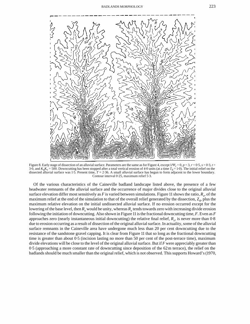
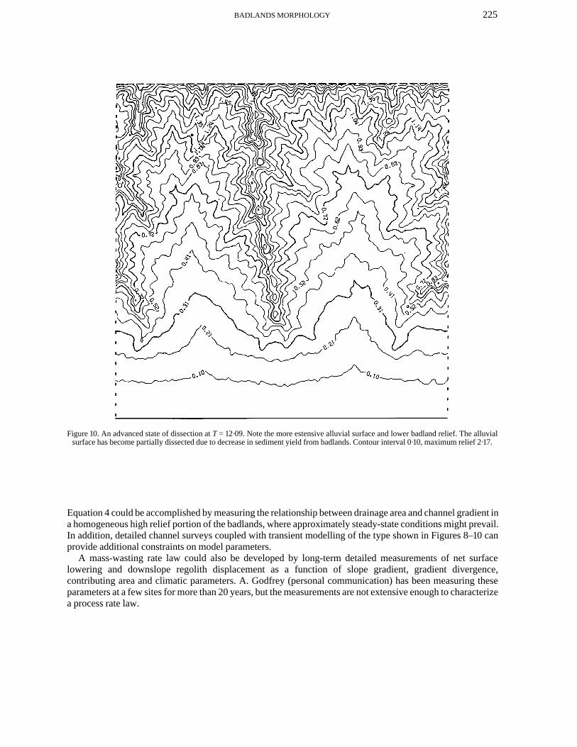
A general pattern of landform evolution emerged from the simulations. In early stages during the constantrate of downcutting, incision occurs first near the base level control (the lower boundary, corresponding to theFremont River), with high relief slopes and steep channels gradually extending further inland (Figure 8,simulated with F = 0·16). Extensive areas of nearly undissected original alluvial surface remain in headwaterareas. Following cessation of downcutting, the downstream channel gradients decline until they reach atransport-limited condition. At this point an alluvial surface develops and extends headward, graduallyreplacing the badland slopes which undergo nearly parallel retreat (Figure 9). In later stages, most of thebadlands are replaced by alluvial surface which is gradually regraded to lower gradient as the sediment yieldfrom the retreating slopes diminishes (Figure 10). Interestingly, the simulation model suggests that the alluvialsurface becomes partially dissected at this stage because of the rapidly diminishing sediment supply.

The maximum relief that develops during the rapid downcutting followed by stability is much less than thesteady-state relief that would be generated by continuing the initial rate of downcutting (the equivalent steady-state topography for Figure 9 is shown in Figure 4); likewise, the drainage density in Figure 9 is higher than thesteady-state case.

The stage of erosion represented by Figure 9 corresponds most closely to the present landform suite in theCaineville area, with about one-third to one-half of the badlands replaced by alluvial surface. Therefore, thecondition of about one-third alluvial surface was used to define the termination time for the simulations, and thecorresponding duration of stable base level Ts, was noted.

223BADLANDS MORPHOLOGY

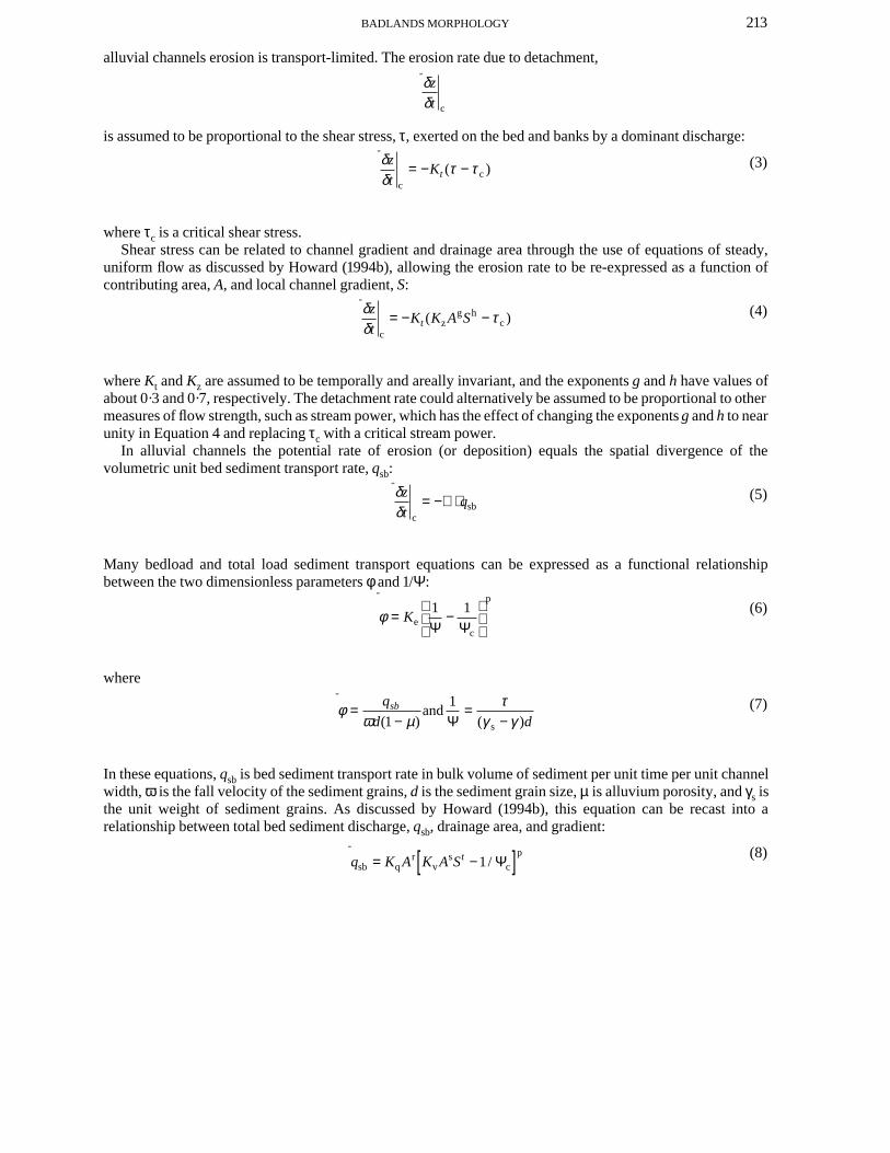
Figure 8. Early stage of dissection of an alluvial surface. Parameters are the same as for Figure 4, except 1/Ψc = 0, p = 3, r = 0·5, s = 0·3, t =3·0, and KqKv = 500. Downcutting has been stopped after a total vertical erosion of 4·0 units (at a time Td = 1·0). The initial relief on thedissected alluvial surface was 1·5. Present time, T = 2·36. A small alluvial surface has begun to form adjacent to the lower boundary.

Contour interval 0·25, maximum relief 5·3.

Of the various characteristics of the Caineville badland landscape listed above, the presence of a fewheadwater remnants of the alluvial surface and the occurrence of major divides close to the original alluvialsurface elevation differ most sensitively as F is varied between simulations. Figure 11 shows the ratio, Rz, of themaximum relief at the end of the simulation to that of the overall relief generated by the dissection, Zd, plus themaximum relative elevation on the initial undissected alluvial surface. If no erosion occurred except for thelowering of the base level, then Rz would be unity, whereas Rz tends towards zero with increasing divide erosionfollowing the initiation of downcutting. Also shown in Figure 11 is the fractional downcutting time, F. Even as Fapproaches zero (nearly instantaneous initial downcutting) the relative final relief, Rz, is never more than 0·8due to erosion occurring as a result of dissection of the original alluvial surface. In actuality, some of the alluvialsurface remnants in the Caineville area have undergone much less than 20 per cent downcutting due to theresistance of the sandstone gravel capping. It is clear from Figure 11 that so long as the fractional downcuttingtime is greater than about 0·5 (incision lasting no more than 50 per cent of the post-terrace time), maximumdivide elevations will be close to the level of the original alluvial surface. But if F were appreciably greater than0·5 (approaching a more constant rate of downcutting since deposition of the 62m terrace), the relief on thebadlands should be much smaller than the original relief, which is not observed. This supports Howard’s (1970,

224 A. D. HOWARD

Figure 9. A later stage of evolution from Figure 8 at a total elapsed time T = 6·24 with a stable base level. Note headward extension ofalluvial surface. Contour interval 0·21, maximum relief 4·5.

1986) conclusion that initial incision was rapid, followed by an appreciable period of time with the river close toits present elevation. It also suggests that the maximum rates of river incision and induced erosion in thebadlands bordering the river exceed the long term of 700mm ka−1 by a factor of 2 to 4. Because the pluvialalluvial surface was mantled with up to 3m of sandstone gravel derived from erosion of the caprock of theCaineville Mesas, dissection of the alluvial surface may have lagged, allowing badland divides to remain nearthe original pediment surface level longer than the simulations (which assume uniform erodibility) imply; thatis, the permissible maximum value of F might be somewhat larger than the value of 0·5 inferred by thesimulations.

DISCUSSION

Despite the concordance between the simulation modelling and the field interpretations of erosional history andcontrols on slope morphology, the mutual confirmation of model and field evidence should be considered to bepreliminary. The simulation model process rate laws and model parameters have not been directly validated andcalibrated by field observations. Long-term process observations would be valuable. In particular, rates oferosion in bedrock rills and channels could be measured and related to drainage area, channel gradient, andrainfall history to calibrate an erosion law of the type of Equation 4. A partial calibration of the exponents of

225BADLANDS MORPHOLOGY

Figure 10. An advanced state of dissection at T = 12·09. Note the more estensive alluvial surface and lower badland relief. The alluvialsurface has become partially dissected due to decrease in sediment yield from badlands. Contour interval 0·10, maximum relief 2·17.

Equation 4 could be accomplished by measuring the relationship between drainage area and channel gradient ina homogeneous high relief portion of the badlands, where approximately steady-state conditions might prevail.In addition, detailed channel surveys coupled with transient modelling of the type shown in Figures 8–10 canprovide additional constraints on model parameters.

A mass-wasting rate law could also be developed by long-term detailed measurements of net surfacelowering and downslope regolith displacement as a function of slope gradient, gradient divergence,contributing area and climatic parameters. A. Godfrey (personal communication) has been measuring theseparameters at a few sites for more than 20 years, but the measurements are not extensive enough to characterizea process rate law.

226 A. D. HOWARD

Figure 11. Relationship between relief and rate of initial incision for simulated dissection of alluvial surface. The ‘relative elapsed timeduring downcutting’ is the fractional downcutting time, F, of Equation 16. The simulations for various values of F are stopped after about

one-third of the total area becomes covered by new alluvial surface. The fractional final maximum relief, Rz, is explained in the text.

REFERENCES

Ahnert, F. 1976. ‘Brief discription of a comprehensive three-dimensional process-response model of landform development’, Zeitschriftfur Geomorphologie, Supplementband, 25, 29–49.

Ahnert, F. 1987. ‘Process–response models of denudation at different spatial scales’, Catena, 10, 31–50.Anderson, R. S., Repka, J. L. and Dick, G. S. 1996. ‘Explicit treatment of inheritance in dating depositional surfaces using in situ 10Be and

26Al’, Geology, 24, 47–51.Carson, M. A. 1971. An application of the concept of threshold slopes to the Laramie Mountains, Wyoming, Institute of British

Geographers Special Publication, 3, 31–47.Carson, M. A. and Petley, D. D. 1970. ‘The existence of threshold slopes in the denudation of the landscape’, Transactions of the Institute

of British Geographers, 49, 71–95.Culling, W. E. H. 1960. ‘Analytical theory of erosion’, Journal of Geology, 68, 336–344.Culling, W. E. H. 1963. ‘Soil creep and the development of hillside slopes’, Journal of Geology, 71, 127–161.Flint, R. F. and Denny, C. S. 1958. ‘Quaternary geology of Bounder Mountain, Aquarius Plateau, Utah’, US Geological Survey Bulletin,

1061-D, 103–164.Gilbert, G. K. 1880. Report on the Geology of the Henry Mountains, US Geographical and Geological Survey, Washington, DC.Hirano, M. 1975. ‘Simulation of developmental process of interfluvial slopes with reference to graded form’, Journal of Geology, 83, 111–

123.Howard, A. D. 1970. A Study of Process and History in Desert Landforms near the Henry Mountains, Utah, unpublished PhD dissertation,

Johns Hopkins University.Howard, A. D. 1971a. ‘Simulation of stream networks by headward growth and branching’, Geographical Analysis, 3, 29–50.Howard, A. D. 1971b. ‘Simulation model of stream capture’, Bulletin of the Geological Society of America, 82, 1355–1376.Howard, D. D. 1986. ‘Quaternary landform evolution of the Dirty Devil River system, Utah’ (abs.), Geological Society of America

Abstracts with Program, 641.Howard, A. D. 1994a. ‘Badlands’, in Abrahams, A. D. and Parsons, A. J. (Eds), Geomorphology of Desert Environments, Chapman &

Hall, London, 213–242.Howard, A. D. 1994b. ‘A detachment-limited model of drainage basin evolution’, Water Resources Research, 30, 2261–2285.Howard, A. D. and Selby, M. J. 1994. ‘Rock slopes’, in Abrahams, A. D. and Parsons, A. J. (Eds), Geomorphology of Desert

Environments, Chapman & Hall, London, 123–172.Hunt, C. B. 1953. Geology and Geography of the Henry Mountains Region, US Geological Survey Professional Paper 228.Kirkby, M. J. 1971. Hillslope process–response models based on the continuity equation, Special Publication, Institute of British

Geographers, 3, 15–30.Kirkby, M. J. 1980. ‘The stream head as a significant geomorphic threshold’, in Coates, D. R. and Vitek, J. D. (Eds), Thresholds in

Geomorphology, George Allen & Unwin, London, 53–73.Kirkby, M. J. 1984. ‘Modelling cliff development in south wales. Savigear re-viewed’, Zeitschrift fur Geomorphologie, 28, 405–426.Kirkby, M. J. 1985. ‘A model for the evolution of regolith-mantled slopes’, in Woldenberg, M. J. (Ed.), Models in Geomorphology, Allen

& Unwin, Boston, 213–237.Kirkby, M. J. 1986. ‘A two-dimensional simulation model for slope and stream evolution’, in Abrahams, A. D. (Ed.), Hillslope Processes,

Allen & Unwin, Boston, 203–222.

227BADLANDS MORPHOLOGY

Kirkby, M. J. 1994. ‘Thresholds and instability in stream head hollows: a model of magnitude and frequency for wash’, in Kirkby, M. J.(Ed.), Process Models and Theoretical Geomorphology, John Wiley & Sons, Chichester, 295–314.

Laronne, J. B. 1981. ‘Dissolution kinetics of Mancos shale-associated alluvium’, Earth Surface Processes and Landforms, 6, 541–552.Laronne, J. B. 1982. ‘Sediment and solute yield from Mancos Shale hillslopes, Colorado and Utah’, in Bryan R. and Yair, A. (Eds),

Badland Geomorphology and Piping, Geo Books, Norwich, 181–192.Morrison, R. B. 1991. ‘Introduction’, in Morrison R. B. (Ed.), Quaternary Non Glacial Geology: Conterminous U.S., Geological Society

of America, Geology of North America, K-2, 1–12.Moseley, M. P. 1973. ‘Rainsplash and the convexity of badland divides’, Zeitschrift fur Geomorphologie, Supplementband, 18, 10–25.Phillips, L. F. 1987. ‘Effect of regional slope on drainage networks’, Geology, 15, 498–521.Schumm, S. A. 1956. ‘Evolution of drainage systems and slopes in badlands at Perth Amboy, New Jersey’, Bulletin of the Geological

Society of America, 67, 597–646.Schumm, S. A., Mosley, M. P. and Weaver, W. E. 1987. Experimental Fluvial Geomorphology, John Wiley & Sons, New York, 413 pp.Smith, J. F. Jr, Huff, L. C., Hinrichs, E. and Luedke, R. G. 1963. Geology of the Capital Reef area, Wayne and Garfield Counties, Utah, US

Geological Survey Professional Paper, 363, 102 pp.Willgoose, G., Bras, R. L. and Rodriguez-Iturbe, I. 1991a. ‘A coupled channel network growth and hillslope evolution model, 1, Theory’,

Water Resources Research, 27, 1671–1684.Willgoose, G., Bras, R. L. and Rodriguez-Iturbe, I. 1991b. ‘A coupled channel networth growth and hillslope evolution model, 2,

Nondimensionalization and applications’, Water Resources Research, 27, 1685–1696.Zernitz, E. R. 1932. ‘Drainage patterns and their significance’, Journal of Geology, 40, 498–521.