Bacteria Growth, Persistence, and Source Assessment in Rural Texas Landscapes and StreamsFinal Report

Texas Water Resources Institute TR-489 November 2015

Lucas Gregory, R. Karthikeyan, Terry Gentry, Daren Harmel, Kevin Wagner, Roel Lopez

Bacteria Growth, Persistence, and Source Assessment in Rural Texas Landscapes and Streams Final Report

Project Funded by:

Texas State Soil and Water Conservation Board: Project 13-56

Investigating Agencies:

Texas A&M AgriLife Research, Dept. of Bioligical and Agricultural Engineering1

Texas A&M AgriLife Research, Dept. of Soil and Crop Sciences2

Texas A&M AgriLife Research, Texas Water Resources Institute3

Texas A&M Institute of Renewable Natural Resources4

U.S. Dept. of Agriculture - Agricultural Research Service5

Prepared by:

Lucas Gregory1,3, R. Karthikeyan1, Terry Gentry2, Daren Harmel5, Kevin Wagner3,

and Roel Lopez4

Texas Water Resources Institute Technical Report TR-489

November 2015

Funding support for this project was provided through a State Nonpoint Source Grant from the Texas State Soil and Water Conserva-tion Board

~ i ~

Bacteria Growth, Persistence, and Source Assessment in Rural Texas Landscapes and Streams

Final Report

Funded by:

Texas State Soil and Water Conservation Board Project 13-56

Investigating Agencies:

Texas A&M AgriLife Research, Dept. of Biological and Agricultural Engineering1

Texas A&M AgriLife Research, Dept. of Soil and Crop Sciences2

Texas A&M AgriLife Research, Texas Water Resources Institute3

Texas A&M Institute of Renewable Natural Resources4

U.S. Dept. of Agriculture – Agricultural Research Service5

Prepared by:

Lucas Gregory1, 3, R. Karthikeyan1, Terry Gentry2, Daren Harmel5, Kevin Wagner3, and Roel Lopez4

Texas Water Resources Institute Technical Report TR-489 November 4, 2015

Funding Support for this project was provided through a State Nonpoint Source Grant from the Texas State Soil and Water Conservation Board

~ ii ~

Table of Contents List of Figures ................................................................................................................................ iii List of Tables ................................................................................................................................. iii List of Acronyms ........................................................................................................................... iv

Abstract ........................................................................................................................................... 1

Instream E. coli Growth and Persistence Assessment .................................................................... 2

Materials and Methods ................................................................................................................ 3

Mesocosm Establishment........................................................................................................ 3

Treatment Scenarios................................................................................................................ 4

Sampling Procedures .............................................................................................................. 5

Analytical Methods ................................................................................................................. 5

Data Analysis .......................................................................................................................... 6

Results ......................................................................................................................................... 6

E. coli Decay Constants .......................................................................................................... 6

E. coli Response to Treatments ............................................................................................... 7

Discussion and Conclusions ....................................................................................................... 8

E. coli Source Assessment on Varying Land Use and Cover Types ............................................ 13

Methods..................................................................................................................................... 15

Site Description ..................................................................................................................... 15

Camera Trapping .................................................................................................................. 16

Small Mammal Trapping ...................................................................................................... 18

Meso-mammal Trapping ....................................................................................................... 18

Avian Trapping ..................................................................................................................... 19

Know Source Fecal Sample Collection ................................................................................ 19

Soil Sampling ........................................................................................................................ 20

Runoff Sample Collection..................................................................................................... 21

E. coli Enumeration and Isolation ......................................................................................... 21

BST – ERIC RP .................................................................................................................... 21

Data Analysis ........................................................................................................................ 22

Results ....................................................................................................................................... 22

Camera Trapping .................................................................................................................. 22

Physical Trapping ................................................................................................................. 24

~ iii ~

Soil E. coli Concentrations ................................................................................................... 27

Runoff E. coli Concentrations ............................................................................................... 28

Soil BST Findings ................................................................................................................. 29

Runoff BST Findings ............................................................................................................ 30

Discussion and Conclusions ..................................................................................................... 34

Education and Outreach ................................................................................................................ 35

References ..................................................................................................................................... 37

Appendix A: Decay Constant Plots .............................................................................................. 40

List of Figures

Figure 1: Decay constant development example for E. coli under varying treatment and flow scenarios .............................................................................................................................. 7

Figure 2: E. coli response in all scenarios and to nutrient amendments alone ............................... 9 Figure 3: E. coli response to flow rate .......................................................................................... 10 Figure 4: Game camera locations and deployment dates .............................................................. 17 Figure 5: Box and whisker plots of E. coli concentrations for all runoff samples collected ........ 28 Figure 6: Identification of E. coli isolates (n=195) from GSWRL soils presented as a 3-way split

(L) and 7-way split (R) ..................................................................................................... 31 Figure 7: E. coli identification of runoff isolates (n=300) using 3-way (L) and 7-way (R) splits 32

List of Tables Table 1. Range of calculated E. coli decay constants under varying treatment scenarios .............. 7 Table 2: Species Richness and Abundance Data from GSWRL .................................................. 23 Table 3: Avian species observed at GSWRL ................................................................................ 24 Table 4: Daily E. coli production estimates for sampled animals based on measured E. coli

density and assumed feces production rates ..................................................................... 25 Table 5: Daily E. coli production for observed animals based on measured E. coli density and

assumed feces production rates ......................................................................................... 26 Table 6: Descriptive statistics of soil E. coli concentrations ........................................................ 27 Table 7: Descriptive E. coli statistics for runoff samples (cfu/100 mL) ....................................... 28 Table 8: E. coli identification results for soil and runoff samples from each watershed broken

into 3 and 7-way splits and the relative percent difference in source identification between soil and runoff samples ....................................................................................... 33

~ iv ~

List of Acronyms ANOVA analysis of variance BST bacterial source tracking cfu colony forming units DO dissolved oxygen DOC dissolved organic carbon DON dissolved organic nitrogen ERIC-PCR Enterobacterial Repetitive Intergenic Consensus – Polymerase Chain

Reaction GSWRL Grassland, Soil, and Water Research Laboratory HDPE high density polyethylene LN natural log mTEC membrane-Thermotolerant NAWA Nutrient and Water Analysis Laboratory NH4-N ammonium NO3-N nitrate PBS phosphate buffered saline PO4-P orthophosphate SAML Soil and Aquatic Microbiology Laboratory TAMU Texas A&M University TDN total dissolved nitrogen USDA-ARS U.S. Department of Agriculture – Agricultural Research Service USEPA U.S. Environmental Protection Agency UV ultraviolet

~ 1 ~

Abstract

Bacteria water quality impairments are the most common water quality issue in Texas and are a considerable source of impairments nationally. Fecal indicator bacteria such as Escherichia coli (E. coli) and enterococci derived from birds and mammals are used as a measure of a waterbody’s ability to support contact recreation. Relationships between monitored levels of E. coli and enterococcus have been established with human contraction of a gastrointestinal illness from pathogenic organisms and serve as the basis for water quality standards that protect contact recreation. Stakeholder processes are often undertaken to improve the quality of impaired waters, define pollutant sources, and develop strategies to reduce bacteria loading to streams. Questions are often asked during these processes regarding the fate and transport of these bacteria in various environmental settings, the distribution of E. coli sources across watersheds, and how they respond to changes in water quality. Past research conducted has worked to address these questions; however, additional work is warranted.

Re-created stream mesocosms were used to develop an improved understanding of E. coli fate and transport in the environment under controlled treatment conditions. Nutrient amendments that mimic increases in nutrient concentrations seen from nonpoint source pollutant loadings and wastewater effluent loadings were applied to determine if E. coli concentrations would change as a result of the amendments and alter growth or decay relative to a control mesocosm. No E. coli growth response was observed in any trial, and no significant differences in decay rates were observed either. This suggests that a single nutrient addition to a stream environment is not sufficient to produce a growth response in the ambient E. coli community.

Soil and runoff samples collected from three controlled land uses were processed to enumerate E. coli and allow individual colonies to be isolated and fingerprinted for bacteria source tracking (BST). E. coli source contributions to native prairie, managed hay pasture, and cultivated cropland sites were determined using 7-way source identification splits. In all cases, wildlife were found to be the primary E. coli contributor. Unexpectedly, cattle and humans were identified as sources of E. coli in runoff and soils from some of the sites. Cattle are not actively stocked nor have they been stocked at any of these sites for at least three years, and no known sources of human fecal deposition have occurred in these watersheds. This demonstrates the complex diversity of E. coli in unimpacted environments and the potential for bacteria to be translocated by transmission vectors.

~ 2 ~

Instream E. coli Growth and Persistence Assessment

Bacteria impairments have been and continue to constitute the bulk of individual waterbody impairments in Texas. As illustrated in the 2012 Texas Water Quality Inventory and 303(d) List, 568 impairments are documented in Texas and 273 of those are attributed to bacteria. This represents roughly 48% of all waterbody impairments in the state. The 2014 Texas Integrated Report illustrates similar levels of bacteria impairments, further emphasizing the need to better understand the sources and fate of bacteria in watersheds so that these impairments can be effectively addressed and managed.

One type of tool that watershed managers currently use is computer-based modeling that

predicts bacteria loading and transport throughout a watershed based on various input parameters. Factors driving E. coli population dynamics (i.e. occurrence, growth, persistence) and transport of bacteria in these models are often sourced from empirical data produced in unrealistic laboratory based experiments; thus, the validity of models used for this purpose is often questioned due to uncertainty in their data inputs (Harmel et al., 2010).

Despite being studied for decades, shortcomings exist in knowledge of Escherichia coli (E.

coli) fate and transport in the environment. Initial determinations from early studies noted that these indicator organisms only existed in the gastrointestinal tracts of warm-blooded animals or their freshly excreted fecal material (Savageau, 1983). This dogma regarding E. coli’s reliance on the intestinal tract of warm-blooded animals for survival led to its widespread use as an indicator of fecal contamination in the environment. In surface waters, the presence of E. coli is assumed to denote recent direct or indirect deposition of fecal material. Numeric criteria have also been established relating the number of E. coli present per 100 mL of water to the risk for human contraction of a gastro-intestinal illness. In most cases, an E. coli level of 126 colony forming units (cfu) per 100 mL of water is applied to waters for primary contact recreation uses (swimming, wading by children, diving, etc.). At this level, it was determined that eight individuals out of every 1,000 engaging in contact recreation are expected to contract a gastro-intestinal illness (Dufour and Ballentine, 1986); therefore, ensuring a complete understanding of E. coli fate and transport in surface waters is crucial for determining the real human health risk from water ingestion.

Recent work has shown that E. coli can persist and grow outside of their host in both soil and

water (Bolster et al., 2005; Garzio-Hadzick et al., 2010; Habteselassie et al., 2008; Ishii et al., 2006; Vital et al., 2008; Wanjugi and Harwood, 2013), thus jeopardizing their effectiveness as accurate indicators of fecal contamination and spawning questions regarding the real risks to human health. To better understand the life cycle of E. coli in the environment, or secondary environments (Savageau, 1983), evaluations of survival and regrowth over extended periods of time in real, or near real environments are needed. It has been hypothesized that nutrient

~ 3 ~

amendments are responsible for observed increases in E. coli concentrations in evaluated water samples. In sterilized environments, this hypothesis has been proven true; however, this hypothesis has not been tested in unaltered stream waters. To improve understanding of E. coli survival in secondary environments, this project employed re-created stream environments to monitor changes in E. coli levels observed in response to varying treatment scenarios.

Materials and Methods

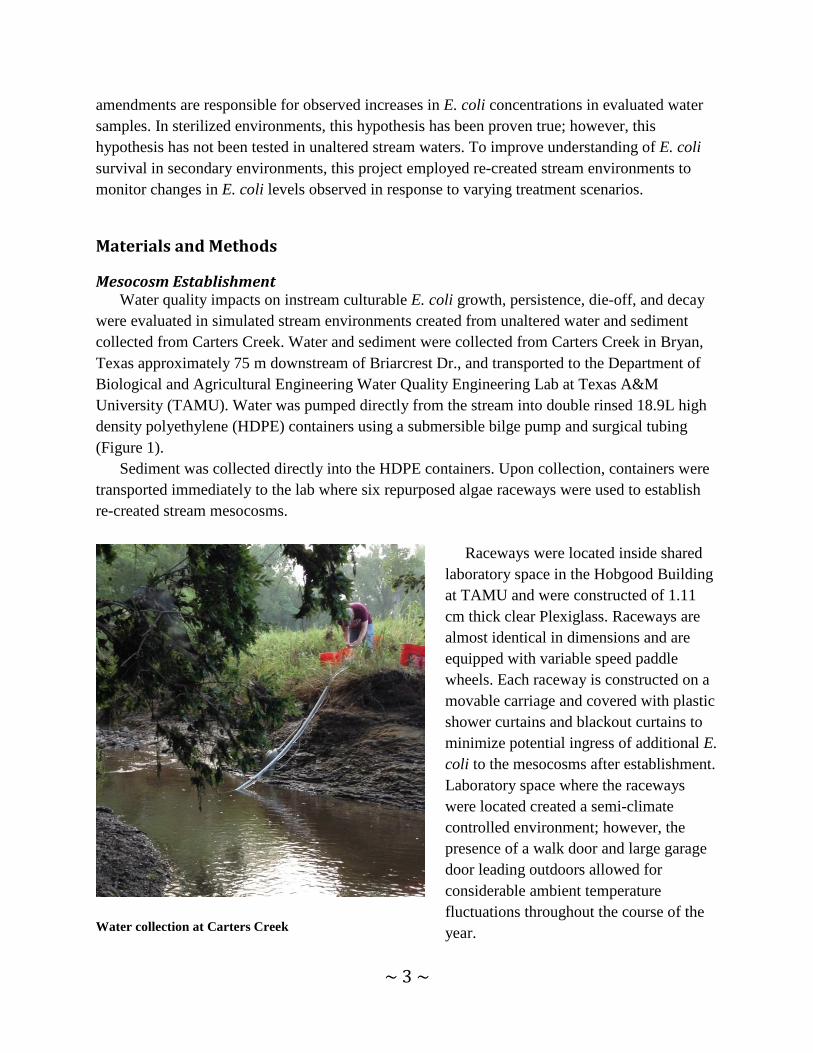
Mesocosm Establishment Water quality impacts on instream culturable E. coli growth, persistence, die-off, and decay

were evaluated in simulated stream environments created from unaltered water and sediment collected from Carters Creek. Water and sediment were collected from Carters Creek in Bryan, Texas approximately 75 m downstream of Briarcrest Dr., and transported to the Department of Biological and Agricultural Engineering Water Quality Engineering Lab at Texas A&M University (TAMU). Water was pumped directly from the stream into double rinsed 18.9L high density polyethylene (HDPE) containers using a submersible bilge pump and surgical tubing (Figure 1).

Sediment was collected directly into the HDPE containers. Upon collection, containers were transported immediately to the lab where six repurposed algae raceways were used to establish re-created stream mesocosms.

Raceways were located inside shared laboratory space in the Hobgood Building at TAMU and were constructed of 1.11 cm thick clear Plexiglass. Raceways are almost identical in dimensions and are equipped with variable speed paddle wheels. Each raceway is constructed on a movable carriage and covered with plastic shower curtains and blackout curtains to minimize potential ingress of additional E. coli to the mesocosms after establishment. Laboratory space where the raceways were located created a semi-climate controlled environment; however, the presence of a walk door and large garage door leading outdoors allowed for considerable ambient temperature fluctuations throughout the course of the year.

Water collection at Carters Creek

~ 4 ~

To establish the mesocosms, the

raceways were first disinfected with a 10% bleach solution, double rinsed with deionized water, vacuumed, and allowed to dry completely. Turbid creek water and sediment was collected from Carters Creek and immediately placed inside the raceways. Water was poured from the transport containers directly into the mesocosms up to a 45 L fill line that was determined volumetrically for each individual raceway. Approximately 1 L of saturated sediment by volume was then introduced to complete mesocosm establishment. Paddle wheels were then activated to create continuously flowing conditions in the chambers.

Treatment Scenarios Applied treatment scenarios were

developed based on initial nutrient levels measured in the ambient water from each mesocosm shortly following its establishment. Treatments were designed to provide a one-time influx of nutrients to the mesocosm. A ‘low-dose’ and ‘high-dose’ treatment were calculated to mimic nutrient loading expected from a naturally occurring runoff event or wastewater treatment plant effluent discharge respectively. Nitrate (NO3-N) and orthophosphate phosphorus (PO4-P) were increased by a factor of 10 and 50 in the low and high doses respectively, while dissolved organic carbon (DOC) was increased by a factor of two and four under each dosing scenario.

Treatments were applied on day two of each trial, approximately 24 hours post mesocosm

establishment. Two mesocosms serve as controls, two receive a ‘low dose,’ and two receive a ‘high dose.’ Additionally, low and high flow rates (approximately 0.2 ft/s and 0.8 ft/s respectively) were applied to a single control, ‘low dose,’ and ‘high dose’ mesocosms.

Algae raceway repurposed for creation of stream mesocosm

~ 5 ~

Sampling Procedures Mesocosm sampling started immediately following mesocosm establishment (Day 0) and

occurred at approximately the same time of day on days 1, 2, 3, 4, 7, 10, 14, 18, and 22. Each sampling day, water and sediment samples were collected directly from each mesocosm and were processed to determine levels of culturable E. coli per 100 mL of water and gram of sediment. Water samples were collected directly from the mesocosms into sterile 500 mL HDPE sample bottles placed into the flow of the mesocosm without disturbing underlying sediment. Following water sample collection, sediment was collected from each mesocosm using disposable plastic spatulas. Sediment was removed from multiple locations within the mesocosm and placed into 207 mL Whirl-Pak® bags.

Mesocosm setup inside enclosures

Analytical Methods E. coli in water and sediment were enumerated using the U.S. Environmental Protection

Agency (USEPA) Method 1603 (USEPA, 2006), which is a membrane filtration method that uses modified membrane-Thermotolerant E. coli agar (mTEC). Aliquots of appropriate volume were processed from water samples and results were reported as cfu/100 mL. Sediment samples were prepared for analysis by placing 10g of saturated sediment into sterile specimen cups containing 90 mL of phosphate buffered saline (PBS) solution. Aliquots of appropriate size were processed in identical fashion as water samples. Results are reported as cfu/ wet g of sediment. Samples were processed immediately following collection to determine ambient turbidity, temperature, pH, dissolved oxygen (DO), and specific conductivity levels in each sample. Turbidity was measured with a Hach 2100Q Portable Turbidimeter and reported in nephelometric turbidity units. Temperature, pH, DO, and specific conductivity were measured with a VWR SB90M5 multi-parameter benchtop meter. Readings for each measure are reported in oC, standard units, mg/L, and µS/cm respectively.

NO3-N, ammonium (NH4-N), PO4-P, DOC, total dissolved nitrogen (TDN) were all

determined by the Nutrient and Water Analysis (NAWA) Laboratory at TAMU. Water

~ 6 ~

subsamples were filtered through 0.7µm glass fiber filters and placed in 100mL HDPE sample bottles for transport to the NAWA lab. NO3-N, NH4-N, and PO4-P were measured colorimetrically using a Smartchem Discrete Analyzer while DOC and TDN were measured through Pt-catalyzed, high temperature combustion performed with Shimadzu TOC-VCSH and TMN-1 units. Dissolved organic nitrogen (DON) was calculated by deducting NO3-N and NH4-N from TDN.

Data Analysis Data analysis was conducted to determine if statistically significant differences occurred

within the E. coli concentrations of the soil and water samples collected. Data were evaluated for normality using a Kolmogrov-Smirnov test and were found to be non-normally distributed. As a result, the Kruskal-Wallis test was used to determine if the medians of runoff E. coli concentrations were statistically different. One-way analysis of variance (ANOVA) was applied to test for differences in mean decay rates between treatment scenarios. Statistical analysis was conducted with Minitab 17 software (Minitab, 2015).

Results

A series of five trials were conducted. Differences in treatment arrangements within the available microcosms led to dissimilar conditions within the treatment and control chambers and ultimately prevented direct comparisons of recorded observations between all five trials. The last three trials conducted were performed under identical conditions and allowed for direct comparison of data produced during those trials. Portions of the data produced during the first two trials were comparable to the latter data sets.

E. coli Decay Constants Identifying and quantifying differences in observed growth or decay constants was a focus of

this work and was accomplished by plotting a regression line through the plotted data points. No growth of E. coli was observed over time in any trial; therefore, only decay constants were produced. Table 1 illustrates the range of decay constants observed and the mean of calculated values. The decay rates were divided into two groups: 0 – 7 days and 7 – 22 days. In this approach, the E. coli value recorded on day 7 was used in the calculation of each decay rate constant. This was done to produce decay constants that most appropriately fit the data plotted. Decay constants are the slope of the line fitted through the natural log (LN) of E. coli concentrations recorded over time. Figure 1 provides an example of data produced in a single trial for a single treatment. All plots are provided in Appendix A.

Separate one-way ANOVA tests were conducted on the calculated decay constants for each

treatment scenario in each time frame to determine if their means were statistically similar to the others. The assumption of normal data distributions was supported in Kolmogrov-Smirnov tests. Results provided evidence that the null hypothesis that all means are equal could not be rejected

~ 7 ~

Treatment Scenario 0 - 7 days 7 - 22 daysControl - Low Flow -0.9193 to -0.8216 (-0.8791)* -0.0345 to 0 (-0.0115)Control - High Flow -0.9599 to -0.4018 (-0.7437) -0.2548 to 0 (-0.1030)High Nutrient - Low Flow -1.0158 to -0.7229 (-0.8623) -0.1293 to 0 (-0.0861)High Nutrient - High Flow -1.0433 to -0.4481 (-0.6952) -0.1623 to 0 (-0.107)Low Nutrient - Low Flow -0.9342 to -0.6982 (-0.7918) -0.1169 to 0 (-0.0623)Low Nutrient - High Flow -1.0541 to -0.4697 (-0.749) -0.2084 to 0 (-0.1115)* range and (mean) of calculated values

Calculated E. coli Decay Constants k (d-1)

for the decay constants in the 0 – 7 day time frame (p=0.904 at α=0.05) and the 7 – 22 day time frame (p=0.516 at α=0.05). Application of a Kruskal-Wallis test supported this finding as well and produced p values of 0.970 and 0.655 respectively.

Table 1. Range of calculated E. coli decay constants under varying treatment scenarios

Figure 1: Decay constant development example for E. coli under varying treatment and flow scenarios

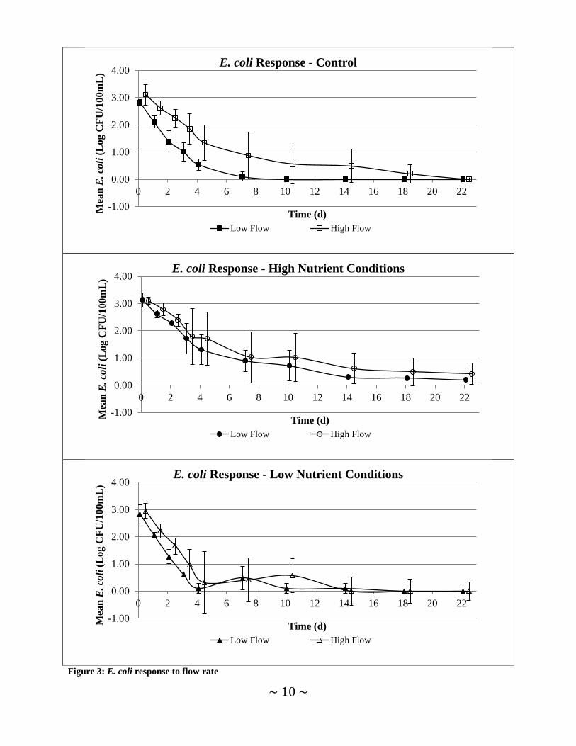
E. coli Response to Treatments E. coli response to applied nutrient and flow rate scenarios was evaluated by incrementally recording E. coli concentrations (Figures 2 and 3). Subtle differences in observed E. coli concentrations occurred in all treatment scenarios but provided little evidence that a particular treatment caused E. coli concentrations to vary considerably from other treatments. Grouping

y = -0.5942x + 7.3874R² = 0.9623

y = -0.1623x + 4.3905R² = 0.8007

0

1

2

3

4

5

6

7

8

0 2 4 6 8 10 12 14 16 18 20 22

E. c

oli (

LN C

FU/1

00m

L)

Time (d)

Trial 3: High Nutrient: High Speed

~ 8 ~

data by flow conditions and comparing nutrient treatments throughout comparable trials revealed little discernable difference in mean E. coli concentrations recorded. When data were grouped by nutrient amendment level and flow rate, more obvious differences were observed. Mean E. coli concentrations recorded under high flow conditions were higher than those recorded on the same day for low flow conditions for all but one sampling event. However, the variability in E. coli concentrations observed was substantial and minimizes the relevance of this finding. A Kruskal-Wallis test was applied to test the hypothesis that median E. coli concentrations observed in each chamber (chambers labeled: C1, C2, L1, L2, H1, H2) on each sampling day in the three comparable trials were the same. Only median E. coli concentrations observed on days 1 and 2 of the trials were found to have statistically significant median values (p=0.023 and p=0.016 respectively). In both cases, the medians for the low flow rate chambers (C1, L1, H1) were significantly lower than the high flow chambers (C2, L2, H2). Visually, days 3 and 4 also appear quite different (Figures 2 and 3); however, their p values were 0.139 and 0.111 respectively. The determination of significance in this case is questionable due to the low sample size for each treatment/chamber combination (n=3).

Discussion and Conclusions

Results from mesocosm evaluations illustrated the survival and decay dynamics of E. coli in simulated, semi-controlled stream environments. The response of E. coli and ambient water quality parameters were systematically recorded to allow for growth and/or decay constants to be established for E. coli over time. A working hypothesis that a single application of nutrient to the mesocosms would produce a response in observed E. coli concentrations was tested. Low and high concentration nutrient amendments failed to produce an E. coli growth response in the water column. Instead, E. coli exhibited a bi-phasic die-off pattern where rapid decay routinely occurred until time 4 or 7 of the trial and was followed by a gradual decay throughout the remainder of the trial (Table 1; Figures 2 and 3). Similar to a multitude of other research, a first-order kinetic decay rate effectively describes the observed decay in all cases. Menon et al. (2003) conducted a similar study using river water mesocosms and observed decay rates ranging from -0.1896 to -0.8136 k (d-1). Craig et al. (2004) used a similar approach to evaluate E. coli persistence in marine waters. Despite the use of differing sampling intervals and initial E. coli concentrations in evaluated waters, similar results were produced in this evaluation. Decay constants exhibited considerable differences. Craig et al. (2004) found T90

values (the amount of time in days that it takes for initial concentrations to be reduced by 90%) to range from 1.12 - 2.22 days where this work produce values ranging from 2.2 - 5.73 days. This difference in both cases is likely a result of non-flowing microcosms versus flowing mesocosms.

~ 9 ~

Figure 2: E. coli response in all scenarios and to nutrient amendments alone

0.00

1.00

2.00

3.00

4.00

0 2 4 6 8 10 12 14 16 18 20 22

Mea

n E

. col

i (L

og C

FU/1

00m

L)

Time (d)

E. coli Response - All Scenarios

Control - Low Flow Control - High Flow Low Nutrient - Low FlowLow Nutrient - High Flow High Nutrient - Low Flow High Nutrient - High Flow

0.00

1.00

2.00

3.00

4.00

0 2 4 6 8 10 12 14 16 18 20 22Mea

n E

. col

i (L

og C

FU/1

00m

L)

Time (d)

E. coli Response - Low Flow Conditions

Control Low Nutrient High Nutrient

0.00

1.00

2.00

3.00

4.00

0 2 4 6 8 10 12 14 16 18 20 22Mea

n E

. col

i (L

og C

FU/1

00m

L)

Time (d)

E. coli Response - High Flow Conditions

Control Low Nutrient High Nutrient

~ 10 ~

Figure 3: E. coli response to flow rate

-1.00

0.00

1.00

2.00

3.00

4.00

0 2 4 6 8 10 12 14 16 18 20 22

Mea

n E

. col

i (L

og C

FU/1

00m

L)

Time (d)

E. coli Response - Control

Low Flow High Flow

-1.00

0.00

1.00

2.00

3.00

4.00

0 2 4 6 8 10 12 14 16 18 20 22

Mea

n E

. col

i (L

og C

FU/1

00m

L)

Time (d)

E. coli Response - High Nutrient Conditions

Low Flow High Flow

-1.00

0.00

1.00

2.00

3.00

4.00

0 2 4 6 8 10 12 14 16 18 20 22

Mea

n E

. col

i (L

og C

FU/1

00m

L)

Time (d)

E. coli Response - Low Nutrient Conditions

Low Flow High Flow

~ 11 ~

These results are quite different from previous work that evaluated E. coli growth potential in sterilized waters. Padia et al. (2012) inoculated sterile water with fecal material from cattle and raccoons and observed growth over a 7-day sampling period. Cattle and raccoon E. coli present in fecal matter incubated in water at 20oC (similar temperature to this work) were found to have growth rates of 1.02 and 1.133 kT (day-1) respectively. UV-treated wastewater effluent spiked with varying concentrations of grass and leaf litter leachate and incubated at 30oC was used as a growth medium by McCrary et al. (2013). Over a 3-day sampling period, they observed net E. coli growth with growth rates ranging from 0.9105 - 3.1325 kT (day-1). This difference in findings between this project and others is not surprising though, as the potential effects of competition and predation from other members of the microbial community were largely mitigated in the referenced works but were not in this project. Research such as that conducted by Wanjugi and Harwood (2013), Oliver et al. (2006), Menon et al. (2003) and others suggests and substantiates the effects of competition and/or predation on the net die-off of E. coli observed in the water column over time. Practically, the results presented here provide an improved resource for use in predictive watershed modeling efforts. Decay constants calculated from observed E. coli concentrations in these simulated stream environments provide information that is likely a better representation of conditions in a real watershed. If used in watershed models, they will improve the predictive capabilities of watershed models in similar watersheds with similar environmental conditions. In theory, models using improved decay rates and transport mechanisms will produce more accurate representations of past and future E. coli loading and also provide better capabilities for assessing management practices. These results are by no means exhaustive but do provide additional information for consideration by the modeling community. Project results also provide evidence that nutrient loading to a waterbody alone is not responsible for frequently observed increases in E. coli concentrations in streams downstream of nutrient loading areas such as wastewater effluent, irrigation return flows or others. The addition of nutrients to a waterbody obviously provides a food source for E. coli and all other heterotrophic microorganisms and thus can support their growth. However, E. coli are typically far outnumbered by heterotrophs. Sandrin (2009) reported total heterotrophic bacteria concentrations in water to range from a low of 101 organisms per mL in spring water to a high of 109 organisms per mL in flowing stream and rivers; E. coli typically make up less than 1% of all heterotrophs in water. Byappanahalli and Fujioka (2004) provided similar evidence and found that the ratio of heterotrophic bacteria to E. coli in Hawaiian soils ranges from 7.31x105 – 2.28x107 to 1. They suggested that heterotrophs other than E. coli are able to effectively use available nutrients more readily than E. coli and as a result, suppress their proliferation. Differences between primary and secondary environmental conditions such as temperature, moisture, and many others experienced by E. coli are stressors (Ishii et al., 2010) to the cells and may also contribute to their delayed response to nutrient amendment.

~ 12 ~

Collectively, these results will improve the ability of watershed managers and the scientific community to evaluate E. coli fate in aquatic environments. Models developed to reflect and predict E. coli loads in watershed systems can be improved by using developed decay constants for flowing, simulated stream conditions. As a result, management scenario modeling will also be improved and provide more realistic results that will aid watershed managers in selecting appropriate mixtures and quantities of management practices to achieve needed loading reduction goals. This study does have several limitations though. The simulated stream environments used in this study did not truly reflect real conditions. Solar radiation and associated UV disinfection were completely excluded and temperature fluctuations were likely greater than they would be in a creek. These effects likely influenced the observed rates of decay; however, the extent to which they influenced the outcomes of this work is unknown. Additionally, creek water and sediment used in this study were collected from a single location and is thus not representative of numerous creeks and rivers. Lastly, true replication of these trials is not possible due to the changing quality of water and sediment between trials. Additional research evaluating other water sources and other treatment scenarios is needed to further the understanding of E. coli decay in flowing water.

~ 13 ~

E. coli Source Assessment on Varying Land Use and Cover Types

Appropriately identifying sources of E. coli and determining their relative contributions to the overall load in a watershed are the first steps to effectively manage E. coli concentrations in a waterbody. Traditionally, watershed surveys, stakeholder input, and published data regarding human and animal populations have provided the bulk of information regarding potential contributors to the overall E. coli load in a watershed. Using these methods, humans, livestock, and larger wildlife ultimately garner much of the attention during planning processes to mitigate E. coli loads since they are readily quantified. Through this approach, many potential E. coli sources in a watershed are overlooked and stakeholders often question the quantity of contributions from ‘background’ or natural sources, as they can and often do represent a considerable portion of the overall load within a given watershed. Other methods of investigation are needed to more completely define the potential sources of E. coli contributions in any watershed.

Bacteria source tracking (BST) is one suite of methods that has been used to identify the

presence or absence, and in some cases the relative contribution, of E. coli from various sources in many watersheds. Conceptually, BST is intended to identify specific characteristics of targeted organisms within environmental samples that are assumed to directly relate back to a known host species or species category (e.g. livestock, wildlife, etc.) (Field and Samadpour, 2007). E. coli is a common organism used in BST as it has direct regulatory significance, is known to correlate to gastrointestinal illness probability and is relatively easy to culture (Jones et al., 2009). BST methods can generally be divided into genotypic or phenotypic approaches, where the former identifies specific DNA sequences within the sample and the latter quantifies an expressed trait observed within the sample such as the ability to consume carbon substrates. BST methods can also be further divided into library-dependent techniques that require the establishment of a library that contains DNA finger prints of E. coli isolated from known animal sources, whereas library-independent approaches use genetic markers that have been developed and have a proven association with known pollutant sources (Stoeckel and Harwood, 2007). A number of BST methods exist and no single approach is superior to others; however, the science continues to evolve and improve (Dick et al., 2010; Field and Samadpour, 2007). Even in best case scenarios, BST is still not able to identify all host sources of E. coli from environmental samples with complete confidence. The availability of known sources of DNA to compare environmental samples to for library-dependent methods is often limited and genetic markers have only been developed for a small number of species.

Runoff water samples collected from experimental watersheds at the U.S. Department of

Agriculture-Agricultural Research Service (USDA-ARS) Grassland, Soil, and Water Research Laboratory (GSWRL) near Riesel, Texas have been analyzed for E. coli, and concentrations vary widely and often exceed surface water quality standards set for E. coli in Texas (126 cfu/100

~ 14 ~

mL) (Harmel et al., 2010; Wagner et al., 2012). Several monitored watersheds had no known contributions of non-wildlife generated (e.g.: human, livestock, litter/waste application) bacteria sources; however, E. coli concentrations from these watersheds were often similar to those from watersheds with known E. coli contributions. These findings further justify the question regarding the contribution of ‘background’ or natural sources of E. coli present in a watershed. This facility provides an excellent setting to investigate this question, as management of the watersheds at the facility ranges from truly native prairie with no human inputs to intensive livestock grazing and other planned manure amendments provides a variety of landscapes to evaluate in one location.

Anecdotal evidence from staff at the GSWRL indicates the presence of several specific

wildlife species and larger species categories. Abundance and distribution of noted species across the sites cannot be quantified from this information though, and no recorded animal use data exist for these small catchments. Thus, ‘natural’ sources are the only expected direct contributors of E. coli to these watersheds; however, the specific sources remain unknown. Methods to identify species’ presences and relative abundances as well as their actual contributions of E. coli are needed to better understand the overall bacteria loading to any landscape.

Identifying the presence or absence of species within a survey area can be accomplished through a variety of approaches that range considerably in equipment costs, labor involvement, time requirements, and effectiveness depending on project goals, objectives, and species targeted. Reported methods used to survey large and medium mammals include aerial survey, drive counts, road census, spotlight census, track counts, pellet group counts, mark recapture techniques, harvest surveys, browse surveys, thermal infrared imagery, road kill counts, remote cameras, hair snares, and scat surveys (Martin, 2009). Survey techniques proven most effective for small mammals were found to be different from those most effective for large mammals. This is primarily due to the difference in ability to directly observe the animals. Trapline transects and pitfall traps are the two small mammal techniques considered most effective (Martin, 2009).

To provide the information needed to better determine the specific sources contributing to the

overall E. coli load observed at GSWRL, a multi-faceted approach was used. Motion sensing game cameras paired with physical animal trapping techniques were used to document the species present at each site. Fecal sample collection from these known sources was also conducted where possible with focus placed on small and meso-mammals. Lastly, known DNA sources were integrated into Texas’ statewide BST library and soil and water samples collected from each plot were compared to this library to determine the source of E. coli in the samples.

~ 15 ~

Methods

Site Description The GSWRL is located near Riesel, Texas in the heart of the Texas Blackland Prairie. This

facility was established in late 1937 on a compilation of private and federally owned land. Today, it consists of 340 ha of land within the larger Brushy Creek watershed in the Brazos River basin. The site’s soils are made up entirely of expansive Houston Black clay (a Vertisol) that consists of 17, 28, and 55 % of sand, silt, and clay particles respectively as determined by size. Soils are very slowly permeable when wet but experience extensive crack formation under dry conditions, thus creating preferential flow paths. Mean annual rainfall ranges from 850 - 910 mm (Allen et al., 2005; Arnold et al., 2005; Harmel et al., 2010; Wagner et al., 2012).

Within GSWRL, experimental watersheds designated as SW12, SW17, and Y6 were used in this assessment. SW12 is a 1.2 ha remnant native prairie plot with 3.8 % slope that has been consistently managed since 1948 (Harmel et al., 2006b). Management practices for the sites include mowing or haying interspersed with intermittent herbicide treatments and prescribed burns. Since 1990, the site has been hayed at least once annually except in 2012 and 2013, (management data available online at: www.ars.usda.gov/spa/hydro-data) following a year of historic drought conditions in 2011. Wagner et al. (2012) noted that no livestock grazing has occurred since at least 1937. The plot lies within a larger nine ha remnant prairie pasture but is hydrologically disconnected from the surrounding area by an earthen berm approximately 0.5 m high and 1 m wide. North and south of the plot, improved pastures are used for grazing. A 4.6 ha shrub/scrub plot is located approximately 33m ENE of the plot at its closest point. The GSWRL headquarters is adjacent to the plot on its western border and is kept as a manicured lawn.

SW12: Native Prairie

SW17: Managed Hay Pasture

Y6: Cultivated Cropland

SW17 is a 1.2 ha managed hay pasture with 1.8 % slope (Harmel et al., 2006b) that was

planted in Coastal bermudagrass in 1949. Prior to this period, the plot was cropped to cotton, corn, oats, or sorghum, using conventional tillage techniques. Records between 1955 and 1999 do not document specific management activity but do indicate the continuous presence of Coastal bermudagrass exists. From 2000-2010, the site was grazed by cattle at rates ranging from 0.29 - 0.90 ha/AU. Grazing was excluded in late 2010 and since then, the site has been hayed,

~ 16 ~

received herbicide treatments, and received 6.8 metric tons/ha (3 ton/ac) applications of poultry litter in 2011 and 2012 (management data available online at: www.ars.usda.gov/spa/hydro-data) that was composted via small windrows inside poultry barns. The plot lies within a larger 1.72 ha hay pasture and is separated by an earthen berm. Cultivated cropland that is sometimes grazed lies to the north of the plot and grazing pastures surround it to the east, south, and west.

Y6 is a 6.6 ha, terraced, cultivated cropland site with 3.2 % slope (Harmel et al., 2006b) that has been continuously cropped since 1943. Crops produced on this site have included clover, cotton, corn, hay grazer, oats, sorghum, sudangrass, small grain, and wheat. The plot also received intermittent fertilizer and herbicide treatments as needed (management data available online at: www.ars.usda.gov/spa/hydro-data). Surrounding fields consist of additional cultivated cropland to the south and grazed pastures to the east, north, and west.

Camera Trapping Motion-triggered game cameras were used to document the presence and relative abundance

of avian and mammalian species on and adjacent to native prairie (SW12), managed hay pasture (SW17), and cultivated cropland (Y6) sites at GSWRL. A single Moultrie model 880i camera (Moultrie Feeders, Calera AL) equipped with a passive infrared, heat, and movement activated trigger was deployed at each plot. The location, date, time, temperature, and moon phase were imprinted on each photo. Complete camera information can be found on the Moultrie Feeders website at: <http://www.moultriefeeders.com/moultrie-m-880-mini-game-camera>.

Cameras were initially deployed on January 28, 2014 and remained on location and recording until February 17, 2015 for a total of 1,158 camera trap days. Cameras were set approximately 0.3 m above ground level in areas where game trails were identified or the terrain/vegetation provided logical travel corridors. Camera deployment locations were adjusted to improve trapping success (Figure 4). When deployed, several baits were used to attract a variety of animals present to the camera’s field of view. Batteries were replaced and memory cards were retrieved periodically throughout the project’s duration. Vegetation was cut as needed in the camera’s field of view to allow easier animal detection by the camera and improve animal identification success. In at least one case at each monitored site, rapid vegetation growth between mowing led to errant camera triggers, which filled memory cards and led to lost photos due to overwriting captured photos. As such, an untold number of photos were lost and the completeness of the species presence and abundance assessment was diminished.

~ 17 ~

Figure 4: Game camera locations and deployment dates

~ 18 ~

Data storage and processing was conducted in accordance with a methodology developed by Harris et al. (2010). The executable programs ‘ReNamer,’ ‘DataOrganize,’ and ‘DataAnalyze’ were used in this processing and are available free at: http://smallcats.org/index.html. The first two programs name and organize the data as noted by Harris et al. (2010). ‘DataAnalyze’ processes the photos and produces data regarding the number of species observed, distribution of these species across monitoring sites, the number of sites a particular species was observed at, and the relative abundance of each species across all sites. The program also determined if animals observed in a series of photos were the same animal through the application of a 60-minute independence threshold.

Small Mammal Trapping Folding aluminum and galvanized metal Sherman Traps were used to capture small

mammals on each of the three monitored sites (H.B. Sherman Inc., Tallahassee, FL). Live traps measured 7.6 cm wide, 9.5 cm tall, and 30.5 cm long and are effective in capturing rodents. These traps allow for the easy release of the captured animal following identification.

Trapping was conducted in two separate events, one the night of January 27-28, 2014 and the other on September 8-9, 2014. During each event, 150 Sherman Traps were deployed (50 per plot) for a total of 300 trap nights. Traps were set approximately two hours before sunset and retrieved beginning at first light the following morning. Traps were baited with a peanut butter, rolled oats, raisins, and strawberry gelatin mixture. When set, traps were focused in and around each plot in an attempt to maximize trapping success. Trap door openings faced identified rodent trails or suspected burrows. Weather conditions during the winter 2014 event were cold and windy with low temperatures recorded on game cameras reaching -10oC, overcast skies, wind from the north varying between 32 - 48 km/h, and a new moon. During the fall 2014 event, low temperatures reached 23oC, winds were light and variable, and skies were clear with a full moon.

When retrieving traps, successful traps were picked up and held vertically so that one trap door could be opened to identify the rodent species without the rodent escaping. Once the species was identified and noted, the rodent was released by opening one end of the trap and setting it on the ground until the animal exited the trap.

Meso-mammal Trapping Professional Series Tomahawk Live Traps (Tomahawk Live Traps, LLC, Hazelhurst, WI)

with a single trap door and easy release door sized for rabbits (22.89 cm x 22.89 cm x 35.56 cm) and large raccoons (30.48 cm x 30.48 cm x 91.44 cm) were used to trap meso-mammals. Traps were constructed of 14 gauge galvanized wire with 1.27 cm x 2.54 cm grid size. A total of 25 traps were deployed during a single trapping event spanning December 14 – 17, 2014 equating to 75 trap nights. Weather during the trapping event as observed varied from overcast to mostly

~ 19 ~

sunny with a temperature range of 0.5 - 22oC (temperatures recorded from on-site game cameras). The third quarter, or half-moon, occurred on December 14.

Fifteen rabbit traps were set in areas where rabbits and other meso-mammals have been observed or rabbit scat was found. Traps were baited with lettuce leaves, baby carrots, and apple slices. Ten raccoon-sized traps were deployed on defined animal trails and near water resources where meso-mammal signs were observed. Traps were baited with sardines in oil. Both types of traps were camouflaged with vegetation from the surrounding area (grasses, forbs, brush) and a trail of bait was extended from the inside of the trap to the trail or area in front of the trap.

Avian Trapping Avian species were trapped at Fort Hood near Killeen, Texas as a part of their Brown-headed

Cowbird trapping program. This program was used as a surrogate trapping site due to lack of an animal use permit to trap birds at GSWRL and its proximity to the site. Fort Hood is located approximately 85 km to the west-southwest of the GSWRL plots. This site is along the boundary of the Texas Blackland Prairie and the Limestone Cut Plains ecoregions and was assumed to have similar avian species composition to GSWRL. Trapping was conducted on February 9, 2015 using established funnel traps located across Fort Hood. Traps are located in upland grassland areas that are similar in nature to the grasslands in and around GSWRL.

Known Source Fecal Sample Collection Known sources of fecal matter were collected from trapped animals or readily identified

droppings for bacteria source tracking analysis. Sterile fecal sample collection tubes with an integrated scoop (Sarstedt, cat# 80.734.311) were used to collect fecal matter. Rodent fecal matter was collected by emptying the contents of Sherman Traps onto a clean 4-cup coffee filter once the trapped rodent was released. Fecal pellets were picked from the coffee filter and placed in the sample tube. Sample tubes were labelled with sample date, time, location, species, and sampler’s initials prior to sample collection. Once completed, sample tubes were sealed and placed in a cooler with ice and transported to the lab.

Fecal samples from meso-mammals were collected similarly. Upon release of the animal, the trap was moved and the fecal matter remained on the ground where the trap had been located. Fecal matter was collected directly from the ground in these cases using the same approach described previously. Coyote feces were collected in the same fashion from scat identified during trap retrieval. No coyotes were trapped during this trapping campaign. Samples from avian species were collected by removing birds from traps and placing them into clean, white cloth bags and allowing them to defecate in the bag. Samples were then removed directly from the bag with the sterile sample container.

~ 20 ~

Soil Sampling Soil samples were collected from each of

the three GSWRL plots for E. coli enumeration and bacterial source tracking. Samples were collected along transects within each plot, extending upslope from the inlet of flow control structure to the edge of the plot. Sampling locations were randomly spaced along these transects but were targeted to capture the variability of conditions within each plot. Within each plot, sampling locations included the following:

- SW12 (Managed Hay Pasture): interspace between bunch grasses, beneath bunch grasses, beneath stoloniferous grasses

- SW17 (Native Prairie): interspace between bunch grasses, beneath bunch grasses

- Y6 (Cropland): atop terraces, within terrace benches, within rills, interrill areas, below stoloniferous grasses in the grassed waterway leading to the flow control structure

Planned sampling was to occur during two sampling events and yield a total of 75 soil samples, 25 from each site. However, due to lack of culturable E. coli in samples collected during these events, two more sampling events producing 75 additional soil samples were conducted. Sampling events were conducted on March 11, 2014, June 17, 2014, October 20, 2014, and February 17, 2015.

In all cases, excess leaf litter or crop residue was removed from the soil surface when

present. Soil samples were taken to a depth of approximately 5 cm with a 7.62 cm soil sampling probe. Between individual sample collections, the sampler changed latex gloves, residual soil was scraped from the soil probe, the probe was sprayed with 200-proof ethanol and flared with a propane torch. Samples were removed from the probe by hand and placed into sterile 710 mL Whirl-Pak® bags (Nasco, Fort Atkinson, WI). Sample bags were labeled with the plot and sample number. Upon collection, samples were placed in a cooler on ice and transported to the Soil and Aquatic Microbiology Laboratory (SAML) at TAMU for analysis.

Soil sample collection February 17, 2015

~ 21 ~

Runoff Sample Collection Runoff samples were collected from each small watershed using automated ISCO Avalanche

refrigerated samplers (Teledyne-ISCO, Inc., Lincoln, NE). Samplers were programmed to collect samples with each 1.32 mm of volumetric runoff depth produced by the respective plot as it flowed through the flow control structure. Upon each sampler activation, tubing that extended from the sampler unit to the flow control structure was rinsed with ambient water prior to collection of a 50 mL sample. Samples collected were composited into a 16 L bottle (Harmel et al., 2006a; Harmel et al., 2014) and were retrieved from the samplers upon cessation of flow or when a 24-hour sample holding time approached and were then taken to the GSWRL laboratory. Bottles were well mixed prior to subsamples being poured into 532 mL Whirl-Pak® bags. Samples were then held in a refrigerator at the GSWRL until retrieval and delivery to SAML. Samples were transported in a cooler on ice.

E. coli Enumeration and Isolation Once delivered to SAML, E. coli in water and soil were enumerated using the USEPA

Method 1603 (USEPA, 2006), which is a membrane filtration method that uses modified membrane-Thermotolerant E. coli agar (mTEC). Aliquots of appropriate volume were processed from water samples and reported as cfu/100 mL. Sediment samples were prepared for analysis by placing 10g of sediment into sterile specimen cups containing 90 mL of PBS. Aliquots of appropriate size were processed in identical fashion as water samples. Results were reported as cfu/wet g of sediment.

E. coli colonies from processed samples were also selected and isolated for BST analysis and

testing. Colonies were picked with a sterile loop and streaked onto nutrient agar MUG (4-methylumbelliferyl-β-D-glucuronide). Colonies that fluoresce under ultraviolet (UV) light are E. coli. One of these fluorescing colonies is then collected with a sterile loop and transferred into a cryovial containing 1 mL of tryptone soy broth with 20% reagent grade glycerol. Vials are vortexed to resuspend the collected cells in the broth and then flash frozen in liquid nitrogen and stored in a -80oC freezer.

BST – ERIC RP The BST technique used for this project was the combined approach that pairs the

enterobacterial repetitive intergenic consensus-polymerase chain reaction (ERIC-PCR) method with RiboPrinting. ERIC-PCR is a library-dependent BST technique that identifies repeated DNA sequences in the genetic sequence of the E. coli processed. The location and number of these sequences vary by specific strain of bacteria, thus producing distinct banding patterns commonly called a DNA fingerprint (de Bruijn, 1992; Versalovic et al., 1991). Similar to ERIC-PCR, RiboPrinting also produces a genetic fingerprint of the processed E. coli; however, it uses enzyme primers to identify and cut the DNA strand at specific points in the sequence. Selected

~ 22 ~

DNA probes hybridize to ribosomal RNA which yield a distinct, banded DNA fingerprint (Clark, 1997).

DNA fingerprints produced from each unknown sample can then be compared to DNA fingerprints of known species to identify the host source. Automated computer software conducts the similarity assessments by performing multiple statistical analyses to determine the level of similarity between the unknown and potential matching sources. To be considered a match, the unknown and known sample’s DNA fingerprint must be at least 80% similar.

Data Analysis Data analysis was conducted to determine if statistically significant differences occurred

within E. coli concentrations of soil and water samples collected. Data were evaluated for normality using a Kolmogrov-Smirnov test and were found to be non-normally distributed. As a result, the Kruskal-Wallis test was used to determine if the medians of runoff E. coli concentrations were statistically different. A one-way ANOVA was also used to test for differences in means of observed E. coli concentrations. These tests were conducted using Minitab 17 software (Minitab, 2015). The Bray-Curtis dissimilarity index and Pearson’s chi-squared tests were applied using the open source statistical software R to evaluate BST results to identify the presence of differences in E. coli species identified by sites and sampling media (soil and water).

Results

Camera Trapping The camera trapping campaign produced a total of 4,872 photos that contained observable

avian and mammalian species. In total, 12 mammalian species and 19 avian species were observed in game camera photos (Table 2). Personnel observations also noted additional avian species during the course of the project.

Diversity and occurrence of species observed in captured photographs was greatest for SW12

and decreased respectively from SW17 to Y6 (Table 2). In total, 11 mammalian species were identified at SW12 followed by eight at SW17 and only six at Y6. This finding is not surprising as SW12 provides the most diverse habitat as it is covered by native grasses and is situated near a brush dominated area. Consistent food availability is also greatest at SW12 given the variety of plant species present. Y6 and SW17 typically have decreasing levels of cover and forage respectively; however, this can change throughout the year as preparations for planting or harvesting at Y6 and haying at SW17 can rapidly change the level of available resources at each site.

~ 23 ~

Table 2: Species Richness and Abundance Data from GSWRL

Species Individual

Animal Count

Species Richness By Site

# of Sites Where Species

Identified

Relative Abundance

SW12 SW17 Y6

Armadillo 1 0 1 0 1 0.05 Avian 321 84 119 118 3 17.2 Bobcat 8 8 0 0 1 0.43 Cattle 4 0 3 1 1 0.21 Cottontail Rabbit 228 222 6 0 2 12.22 Coyote 174 89 23 62 3 9.32 Deer 24 24 0 0 1 1.29 Dog 8 7 1 0 2 0.43 Feral Cat 12 12 0 0 1 0.64 Jackrabbit 220 2 85 133 3 11.79 Opossum 28 28 0 0 1 1.5 Raccoon 3 2 0 1 2 0.16 Rat 27 18 8 1 3 1.45 Skunk 339 183 95 61 3 18.17 Unknown 469 241 78 150 3 25.13 Total Counts 1,866 920 420 526 NA NA

Table 2 illustrates the number of individual species or species categories (avian) observed

from game camera photos, the number of times they were observed, the sites within GSWRL where they were observed and the abundance of the species relative to others. Unknown individuals comprised the largest number of individual counts and occurred due to the in ability to capture a complete image of the animal. Of the species documented in photos, skunk were the most abundant followed respectively by avian, cottontail rabbit, jackrabbit, coyote, opossum, rat, deer, feral cat, bobcat, dog, cattle, raccoon, and armadillo.

The avian category provides a great deal of uncertainty in this analysis, as there were

numerous cases of more birds than could be accurately counted present in a single photo. In these cases, the species abundance matrix was calculated using a count of five individuals, thus greatly underrepresenting the real number of birds observed. Table 3 includes the 21 species of bird observed at least once in game camera photos and by field staff during the duration of the project.

~ 24 ~

Table 3: Avian species observed at GSWRL Avian Species Observed at GSWRL

Eastern Meadowlark Western Meadowlark Brownheaded Cowbird Loggerhead Shrike Red-tailed Hawk Red-Shouldered Hawk Mourning Dove Turkey Vulture Upland Sandpiper Northern Harrier American Crow Yellow-bellied Flycatcher Black Vulture Killdeer Vesper Sparrow Scissor-tailed Flycatcher Northern Mockingbird Swainson’s Hawk Crested Caracara Great Blue Heron Eurasian Collared Dove

Physical Trapping Physical trapping was conducted through the project primarily as a means to collect known

sources of fecal matter for use in bacterial source tracking analyses. A goal of 50 known sources of fecal matter was collected and added to the Texas E. coli BST Library. Collectively, the trapping efforts yielded a total of 56 known sources of fecal matter.

A total of 300 trap nights targeted toward small mammals produced 19 fecal samples from

White-footed mice and seven fecal samples from Eastern Woodrats for a total 26 samples. This equates to an 8.7% trapping success rate, which is lower than expected due to the physical evidence of rodent activity at all sites. Meso-mammal trapping that was conducted produced similar results. A total of 75 trap nights produced only 11 captures for a trapping success rate of 14.7%. Fortuitously, a coyote was observed from a distance defecating, enabling a fresh fecal sample to be collected. Bird sampling produced similar trap success with 18 samples collected.

E. coli Production Rates

One project goal was to calculate E. coli production rates for wildlife species observed at GSWRL. Ideally, fecal samples from each species observed in camera photos would have been secured; however, this was not the case as samples from only five of the 13 mammalian species observed were obtained. E. coli from each fecal sample were enumerated at SAML using the USEPA 1603 method to produce a concentration in cfu/wet gram of fecal matter. Fecal matter from three avian species was also collected and enumerated. The estimated range of E. coli produced by each animal was then calculated based on the measured E. coli concentration in project specific data or in other findings from BST projects conducted across the state, published ranges of animal body weights, and the assumption that daily fecal production equates to approximately 1% of total body weight. Table 4 presents results from animals sampled through this project while Table 5 presents estimates for animals observed through the project but not sampled.

~ 25 ~

Table 4: Daily E. coli production estimates for sampled animals based on measured E. coli density and assumed feces production rates Common Name Scientific Name Reported

Species Adult Weight Range

Number of Fecal Samples Analyzed

Measured E. coli Production Range

Estimated Range in Daily Feces Production1

Estimated Range in Daily E. coli Production

Mammals (kg) (cfu/wet g) (g/day) (cfu/day) Common Raccoon Procyon lotor 4 - 13 1 7.00 E+06 19.2 - 165.1 1.34 E+08 - 1.16 E+09 Coyote Canis latrans 14 - 20 1 4.80 E+04 133 - 220 6.38 E+06 - 1.06 E+07 Virginia Opossum Didelphis

virginiana 1.8 - 4.5 9 8.00 E+04 - 4.10 E+07 8.64 - 57.2 6.91 E+05 - 2.35 E+09

White-footed Mouse

Peromyscus leucopus

0.018 - 0.032 19 3.00 E+03 - 1.60 E+07 0.086 - 0.406 2.58 E+02 - 6.50 E+06

Eastern Woodrat Neotoma floridana

0.2 - 0.35 7 4.00 E+05 - 1.00 E+08 0.96 - 4.45 3.84 E+05 - 4.45 E+08

Birds (g) House Sparrow Passer

domesticus 27 - 29 1 3.18 E+03 0.130 - 0.368 4.13 E+02 - 1.17 E+03

Red-winged Blackbird

Agelaius phoeniceus

41 - 71 2 1.14 E+03 - 8.08 E+03 0.197- 0.902 2.25 E+02 - 7.29 E+03

Brown-headed Cowbird

Molothrus ater 40 - 50 15 2.54 E+03 - 2.00 E+06 0.192 - 0.635 4.88 E+02 - 1.27 E+06

1Estimated daily fecal production rates estimated using average feces production as a percentage of total body weight. Coyote fecal production assumed similar to cattle due to animal size; range of production as presented by Banta et al. (2011) for beef cattle (0.95 – 1.1%) used. All other species in table assumed to feces at rates described for wild mice by Haines et al. (1973) (0.48 – 1.27%).

~ 26 ~

Table 5: Daily E. coli production for observed animals based on measured E. coli density and assumed feces production rates Common Name Scientific Name Reported

Species Weight Range

Reported E. coli Production Range

Estimated Range in Daily Feces Production*

Estimated Range in Daily E. coli Production

(kg) (cfu/wet g) (g) (cfu/day) Nine-banded Armadillo

Dasypus novemcinctus

4 - 8 2.95 E+05 - 4.98 E+08 19.2 - 101.6 5.66 E+06 - 5.06 E+10

Bobcat Lynx rufus 5 - 9 1.90 E+06 24 - 114.3 4.56 E+07 - 2.17 E+08 Beef Cattle**1 Bos taurus 272 - 1,134 2.81 E+02 - 1.92 E+06 3,800 - 4,400 1.07 E+06 - 8.45 E+09 Dog**2 Canus lupus 1 - 80 1.00 E+02 - 4.80 E+07 171.9 - 249.7 1.72 E+04 - 1.20 E+10 Feral Cat**3 Felis catus 2 - 11 1.50 E+03 - 7.80 E+05 21.6 - 68.6 3.24 E+04 - 5.35 E+07 Striped Skunk Mephitis mephitis 1.4 - 6.6 5.01 E+02 - 7.62 E+04 6.72 - 83.8 3.37 E+03 - 6.39 E+06 White-tailed Deer Odocoileus

virginianus 30 - 70 4.60 E+04 - 2.69 E+07 285 - 770 2.85 E+04 - 3.00 E+11

*Estimated daily fecal production rates estimated using average feces production as a percentage of total body weight. Dog and White-tailed deer fecal production assumed similar to cattle due to animal size; range of production as presented by Banta et al. (2011) for beef cattle (0.95 – 1.1%) used. All other species in table assumed to feces at rates described for wild mice by Haines et al. (1973) (0.48 – 1.27%). ** Extreme variability exists in average weight of specific breeds within the species; extreme weight ranges reported; estimated weights of animals observed utilized in estimated fecal production 1 400 kg yearling on winter cover crop 2 18.1 - 22.7 kg dogs; medium size mix breed 3 4.5 - 5.4 kg tabby cat, normal adult size

~ 27 ~

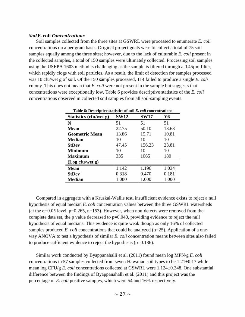
Soil E. coli Concentrations Soil samples collected from the three sites at GSWRL were processed to enumerate E. coli

concentrations on a per gram basis. Original project goals were to collect a total of 75 soil samples equally among the three sites; however, due to the lack of culturable E. coli present in the collected samples, a total of 150 samples were ultimately collected. Processing soil samples using the USEPA 1603 method is challenging as the sample is filtered through a 0.45µm filter, which rapidly clogs with soil particles. As a result, the limit of detection for samples processed was 10 cfu/wet g of soil. Of the 150 samples processed, 114 failed to produce a single E. coli colony. This does not mean that E. coli were not present in the sample but suggests that concentrations were exceptionally low. Table 6 provides descriptive statistics of the E. coli concentrations observed in collected soil samples from all soil-sampling events.

Table 6: Descriptive statistics of soil E. coli concentrations Statistics (cfu/wet g) SW12 SW17 Y6 N 51 51 51 Mean 22.75 50.10 13.63 Geometric Mean 13.86 15.71 10.81 Median 10 10 10 StDev 47.45 156.23 23.81 Minimum 10 10 10 Maximum 335 1065 180 (Log cfu/wet g) Mean 1.142 1.196 1.034 StDev 0.318 0.470 0.181 Median 1.000 1.000 1.000

Compared in aggregate with a Kruskal-Wallis test, insufficient evidence exists to reject a null hypothesis of equal median E. coli concentration values between the three GSWRL watersheds (at the α=0.05 level, p=0.265, n=153). However, when non-detects were removed from the complete data set, the p value decreased to p=0.040, providing evidence to reject the null hypothesis of equal medians. This evidence is quite weak though as only 16% of collected samples produced E. coli concentrations that could be analyzed (n=25). Application of a one-way ANOVA to test a hypothesis of similar E. coli concentration means between sites also failed to produce sufficient evidence to reject the hypothesis (p=0.136).

Similar work conducted by Byappanahalli et al. (2011) found mean log MPN/g E. coli

concentrations in 57 samples collected from seven Hawaiian soil types to be 1.21±0.17 while mean log CFU/g E. coli concentrations collected at GSWRL were 1.124±0.348. One substantial difference between the findings of Byappanahalli et al. (2011) and this project was the percentage of E. coli positive samples, which were 54 and 16% respectively.

~ 28 ~

Runoff E. coli Concentrations The first runoff producing rain event during the project period occurred on October 12, 2013

and the last event occurred on May 30, 2015. Runoff did not occur at all sites during each rain event at GSWRL, resulting in a dissimilar number of samples collected at each site. The slope of SW17 could have factored into runoff production, as its slope is only 1.8%, whereas the slopes of SW12 and Y6 are 3.8 and 3.2% respectively. Distance between sites and non-uniformity in rainfall distribution across the GSWRL were also likely contributors to runoff production.

Similar to the findings of other projects, E. coli concentrations observed exhibited considerable variability (Table 7, Figure 5). Application of the Kruskal-Wallis test provided evidence that the null hypothesis of equal medians can be rejected for these data. Median E. coli values recorded at SW12 were statistically less than those observed at SW17 and Y6 (p=0.033). Each sample set did contain a single high outlier; however, their inclusion did not impact the outcome of this analysis as a Kruskal-Wallis test conducted with outliers removed produced similar results (p=0.025).

Table 7: Descriptive E. coli statistics for runoff samples (cfu/100 mL) Statistics SW12 SW17 Y6 N 25 14 22 Mean 8811 14490 14578 Geometric Mean 1372.1 3425.2 3991.8 Median 1000 5950 4700 StDev 31701 21723 31424 Minimum 160 20 70 Maximum 160000 80000 150000

Figure 5: Box and whisker plots of E. coli concentrations for all runoff samples collected

E. c

oli (

cfu/

100

mL)

101

102

103

104

105

106

SW12 SW17 Y6

~ 29 ~

Soil BST Findings In total, BST was completed on 195 E. coli isolates using the ERIC-RP method. Ideally, the

sample distribution between sites would have been similar; however, roughly 58, 32, and 10% of available E. coli isolates were derived from sites SW17, SW12, and Y6 respectively. This resulted, at least in part, from the low presence of culturable E. coli in the soils and non-equal distribution of E. coli between sites collected during the four sampling events.

Results produced were aggregated by site and summarized using a 3-way and 7-way split for each location (Figure 6, Table 8). Source identifications are based upon the Texas E. coli BST Library, which included 53 known source E. coli isolates collected from GSWRL. Collectively, wildlife was identified as the dominant source of E. coli found in soils from each plot and ranged from 52 - 81%. This finding is expected, as each of these sites is intentionally managed to exclude the additions of E. coli from manageable sources (i.e. livestock, human) thus, the only expected source contributing to these sites is wildlife. Contrary to this finding is the identification of livestock and domestic animals as the second most common source category for SW12 and SW17. Livestock and domestic animals were also identified as contributors to the overall E. coli load at Y6 as well, but unidentified sources were more common in this location. The finding of livestock and domestic animal influences are somewhat surprising given the fact that no animals included in this source category are intentionally allowed onto these sites. However, photos taken from within these plots identified at least a single occasion at each site where livestock (cattle) or domestic animals (dogs) were present. It is not known if these animals contributed any fecal matter during these visits, but their presence makes the contributions from these sources plausible.

Potential sources of unexpected E. coli identified at each site by motion-activated game cameras

Unidentified sources of E. coli were also found from soil samples at each site. The relative percentage of unidentified isolates at sites SW12 and SW17 was ≤5% (n=3 & 2) while 32% (n=6) of isolates from Y6 were attributed to unidentified sources. This is likely due in part to the low number of E. coli isolates produced in soil samples collected from Y6. Human contributions were also identified in 5% (n=3) E. coli isolates collected from SW12. A possible explanation of

~ 30 ~

this finding is translocation of human borne E. coli from the surrounding area via a transmission vector such as a dog, coyote, opossum, or other animal that might have consumed human derived E. coli offsite and later deposited it within the watershed.

Livestock and domesticated animals were further split out into cattle, other livestock (avian), and other livestock (non-avian) while the wildlife category was split into avian and non-avian wildlife. This assessment resulted in cattle being identified as a contributing source in SW12 and SW17 but not Y6. Other avian livestock was only noted in samples from SW12 while other non-avian livestock were identified as a contributor to all sites.

Runoff BST Findings E. coli isolates from runoff samples collected at the three plots were also processed using

ERIC-RP to identify the sources of fecal matter present in each respective watershed. In total, 300 E. coli isolates were typed and compared to the Texas E. coli BST Library. Similar to soil isolates, the distribution and number of isolates available from each site was not consistent with 53, 27, and 20% coming from watersheds SW12, Y6, and SW17 respectively.

Runoff BST results produced findings similar to those found in soil derived E. coli isolates. Wildlife derived sources were dominant at each site with percent compositions ranging from 56 - 70% (Figure 7, Table 8). Livestock and domesticated animals were identified as the second most common source of E. coli in each site with 18 - 39% representation. Unidentified sources were the third most prominent source category with 5 - 10% of E. coli not being attributable to a specific source. Human derived E. coli were found in runoff samples from SW12 and Y6 and comprised 5 and 2% of the total number of isolates at each site respectively.

Refining the wildlife category into avian and non-avian wildlife revealed that non-avian wildlife was identified as the major contributor of E. coli in each watershed (43 – 56%) while avian wildlife contributed only 12 – 14% of the identified E. coli. In all watersheds, the refinement of the livestock and domesticated animals category produced variable results and included occurrences of other livestock (non-avian), cattle, pets, and other livestock (avian). Pet derived E. coli were not identified in any of the soil samples collected; however, the observation of dogs and feral cats with motion-activated cameras makes this a somewhat expected finding.

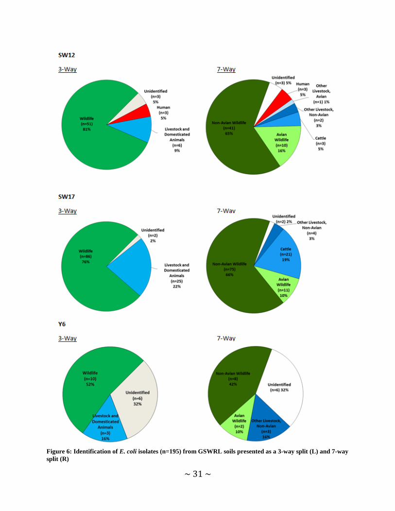
~ 31 ~

Figure 6: Identification of E. coli isolates (n=195) from GSWRL soils presented as a 3-way split (L) and 7-way split (R)

~ 32 ~

Figure 7: E. coli identification of runoff isolates (n=300) using 3-way (L) and 7-way (R) splits

~ 33 ~

Table 8: E. coli identification results for soil and runoff samples from each watershed broken into 3 and 7-way splits and the relative percent difference in source identification between soil and runoff samples

Site Soil Runoff % Difference SW12 3-way 7-way 3-way 7-way 3-way 7-way

Wildlife Avian

81 16

62 12

26.6 28.6

Non-Avian 65 50 26.1

Livestock and Domesticated

Cattle

9

5

24

4

90.9

22.2 Pets 0 9 200 Other Avian 3 2 40 Other Non-Avian

1 8 155.6

Human 5 5 5 5 0 0 Unidentified 5 5 9 9 57.1 57.1

SW17 3-way 7-way 3-way 7-way 3-way 7-way

Wildlife Avian

76 10

56 13

30.3 26.1

Non-Avian 66 43 42.2

Livestock and Domesticated

Cattle

22

19

39

12

55.7

45.2 Pets 0 7 200 Other Avian 0 5 200 Other Non-Avian

3 15 133.3

Human 0 0 0 0 0 0 Unidentified 2 2 5 5 85.7 85.7

Y6 3-way 7-way 3-way 7-way 3-way 7-way

Wildlife Avian

52 10

70 14

28.6 33.3

Non-Avian 42 56 26.3

Livestock and Domesticated

Cattle

16

0

18

6

11.7

200 Pets 0 1 200 Other Avian 0 3 200 Other Non-Avian

16 8 66.7

Human 0 0 2 2 200 200 Unidentified 32 32 10 10 104.8 104.8

No obvious differences in the source composition of E. coli contributions identified through BST analysis between the sampling media (soil and runoff) and between sites were identified. To test for significant differences, a one-way ANOVA was applied to quantify differences in E. coli

~ 34 ~

species composition between sampling media and sampling sites. No significant differences were identified between sampling media and species (wildlife, livestock and domestic, human, unidentified) or between sampling site and species (p>0.162). Similarly, a Pearson’s chi-squared test was applied to test for significant dependence between sampling media or sampling site and E. coli. When applied to sampling media and E. coli, a possible dependence was identified (p= 0.0417). A possible dependence was also identified between sampling sites and species (p= 0.0004); however, it should be noted that the total number of species counts within some sampling sites were quite small and diminished the power of the test.

Discussion and Conclusions

Developing a solid understanding of the sources and relative distribution of E. coli contributions to a watershed is perhaps the most critical step in ultimately managing those sources to reduce their influence on downstream water quality. Traditional methods to determine the E. coli sources produce rough scale estimates for contributions to a watershed and result in obvious sources of fecal loading being identified as the most significant contributing sources. However, these methods are unable to capture the real breadth of contributing sources present within a watershed or specific land uses within the watershed. This often results in potentially large sources of E. coli being poorly understood and managed. Application of long-term game camera trapping and BST within intensively managed micro watersheds allowed an assessment of E. coli sources to be completed and additional knowledge regarding the sources present on a variety of land uses to be improved. Game camera use proved to be an effective means to document the presence and relative abundance of E. coli sources in and near the monitored watersheds. The continuous application of this tool for over a year added great information about the variety of species present. Prior to game camera deployment, the knowledge of contributing E. coli sources was limited to that of personnel managing the sites. While they did note the presence of many of the species observed, the relative abundance of these species and their frequency of occurrence onsite were unknown. Less common species at each site were also not mentioned by personnel and thus not known to use monitored watersheds. These autonomous cameras proved quite effective for documenting species’ presence and usage patterns and for providing relative abundance information for medium and large mammals. Game cameras do have limitations though; small mammals such as mice and rats often are hidden by vegetation or simply do not trigger the camera. Rapid vegetation growth can also result in lost photos thus diminishing the effectiveness of the cameras. Land use and land cover did not appear to produce starkly different BST results in soils sampled, as wildlife was the dominant source identified in all three types. The general lack of E. coli isolates produced from soil samples was more telling though, and suggests that their presence is unlikely to be a result of naturalization into the soil microbial community but is

~ 35 ~

rather more likely related to recent fecal depositions. E. coli concentrations found were similar to other published data such as that of Byappanahalli et al. (2011), who concluded that E. coli were common in soil and should be considered an environmental source of E. coli. Findings from Riesel do not provide substantial support for these claims. A more extensive data collection effort could improve results of this assessment and should be considered in future efforts. Runoff data collected produced greater differences between sites both in terms of observed E. coli concentrations and sources of E. coli identified. As with the findings of many studies evaluating E. coli concentrations and loads, the variability in observed E. coli concentrations was substantial. At each site, the differences in concentrations observed over the course of the study varied by more than three orders of magnitude and indicate that sizeable E. coli concentrations can be found in runoff from any land use. In the aggregate, land use did prove to have a significant effect on the concentrations of E. coli observed. SW12, the native prairie site, had a significantly lower median E. coli concentration than did the managed hay pasture or cultivated cropland (SW17 & Y6). BST results also exhibited a few subtle differences between sites. As expected, wildlife was identified as the dominant source of E. coli present at each site; however, cattle and other livestock were also identified from all sites and human sources were found at all sites but SW17. While cattle-derived E. coli could at least partly be explained by infrequent occurrences of cattle being in the wrong pasture, the other livestock and human sources could not. Transmission vectors, presumably wildlife, provide a possible explanation of these findings. This confounds the task of managing known sources of E. coli loading to a site as these sites are already managed to exclude these sources of E. coli, yet they were identified in collected runoff regardless of applied management efforts. Collectively, E. coli concentrations and BST results from soil and runoff collected from each site also provided insight into the distribution of E. coli sources between sampled media and between sites. Even under a controlled setting such as that at GSWRL, managing a watershed to completely exclude a source of E. coli is difficult at best. Thus, management prescribed to address E. coli loadings should account for these uncertainties and not assume that only the known sources of E. coli in a specific area are the only contributors.

Education and Outreach Delivery of project finding occurred primarily through two avenues: national level

conferences and the project website. Conferences

Preliminary project findings were presented at three national conferences and served as the primary mode of information delivery. At the approximate mid-point of the project period, two presentations were made at the 2014 Water Microbiology Conference held in Chapel Hill, North Carolina on May 5-8, 2014. The first presentation entitled “Identifying Sources and Quantifying

~ 36 ~

Differences in E. coli Occurrence in Soils from Unimpacted Catchments with Varying Landuse” conveyed fecal indicator bacteria derived water quality issues currently faced by water quality managers, sources of bacteria, methods to identify these sources, and provided a general primer on BST prior to providing an overview of the study site, its historic water quality, study design, and preliminary soil BST findings. Discussion was not extensive as results were preliminary, but surprise findings were highlighted and potential justification for these findings were offered. A second presentation was also given at this conference entitled “Assessing Impacts of Nutrient Loading on Culturable E. coli in Re-Created Natural Stream Mesocosms.” This presentation also focused on water quality issues stemming from E. coli and highlighted some of the questions regarding its use as a measure of water quality. Questions from watershed stakeholders regarding E. coli fate and transport in the environment were discussed and provided the significance for the project. The project design and specifics of the sampling strategy were discussed and feedback from the audience was sought for potential improvements to the design. Benefits, limitations, and expected results from the experiment were discussed; however, no preliminary data was available for this discussion. Audiences for these presentations consisted of students, professors, agency personnel, and key experts in the field of water resources-related microbiology. Presentations were attended by 23 and 21 persons, respectively.

A presentation was also given at the American Water Resources Association conference held November 3-6, 2014 in Vienna, Virginia. This presentation was also entitled “Identifying Sources and Quantifying Differences in E. coli Occurrence in Soils from Unimpacted Catchments with Varying Landuse.” Originally, final BST results from the soil sampling campaign were planned for presentation at this conference; however, due to the relative absence of E. coli in soil samples collected during June 2014, no new findings were available for discussion. As a result, the presentation made was nearly identical to the presentation of the same title given at the 2014 Water Microbiology Conference. A total of 27 students, professors, and agency personnel attended this presentation.

Shortly after the conclusion of the project, a final presentation of project results was given at the 2015 Universities Council on Water Resources Conference held in Henderson, Nevada June 15 – 19, 2015. At this conference, a presentation entitled “Assessing Impacts of Nutrient Loading on Culturable E. coli in a Re-Created Natural Stream Mesocosm” was given. Final results from the instream E. coli growth and persistence aspect of the project were given. The need for the project, its design, and the site description were also presented as mentioned earlier in this section. A total of 16 students and professors attended this presentation. Project Website

The project website has also been used as a means to distribute results from the project. Quarterly progress reports, presentations and the project final report are posted at http://bft.tamu.edu. During the project period, a total of 177 unique visitors perused the project website.

~ 37 ~

References Allen, P. M., R. D. Harmel, J. Arnold, B. Plant, J. Yelderman, and K. King. 2005. Field data and flow system response in clay (vertisol) shale terrain, north central Texas, USA. Hydrol. Process. 19(14):2719-2736.

Arnold, J. G., K. N. Potter, K. W. King, and P. M. Allen. 2005. Estimation of soil cracking and the effect on surface runoff in a Texas Blackland Prairie watershed. Hydrol. Process. 19(3):589-603.

Banta, J. P., D. L. Lalman, F. N. Owens, C. R. Krehbiel, and R. P. Wettemann. 2011. Effects of prepartum supplementation of linoleic and mid-oleic sunflower seed on cow performance, cow reproduction, and calf performance from birth through slaughter, and effects on intake and digestion in steers. Journal of Animal Science 89(11):3718-3727.

Bolster, C. H., J. M. Bromley, and S. H. Jones. 2005. Recovery of chlorine-exposed Escherichia coli in estuarine microcosms. Environ. Sci. Technol. 39(9):3083-3089.

Byappanahalli, M. N., and R. Fujioka. 2004. Indigenous soil bacteria and low moisture may limit but allow faecal bacteria to multiply and become a minor population in tropical soils. Water Sci. Technol. 50(1):27-32.

Byappanahalli, M. N., B. M. Roll, and R. S. Fujioka. 2011. Evidence for occurrence, persistence, and growth potential of Escherichia coli and enterococci in Hawaii's soil environments. Microbes Environ.

Clark, C. G. 1997. Riboprinting: A tool for the study of genetic diversity in microorganisms. J. Eukaryot. Microbiol. 44(4):277-283.

Craig, D. L., H. J. Fallowfield, and N. J. Cromar. 2004. Use of microcosms to determine persistence of Escherichia coli in recreational coastal water and sediment and validation with in situ measurements. J. Appl. Microbiol. 96(5):922-930.

de Bruijn, F. J. 1992. Use of repetitive (repetitive extragenic palindromic and enterobacterial repetitive intergeneric consensus) sequences and the polymerase chain reaction to fingerprint the genomes of Rhizobium meliloti isolates and other soil bacteria. Appl. Environ. Microb. 58(7):2180-2187.

Dick, L. K., E. A. Stelzer, E. E. Bertke, D. L. Fong, and D. M. Stoeckel. 2010. Relative decay of Bacteroidales microbial source tracking markers and cultivated Escherichia coli in freshwater microcosms. Appl. Environ. Microb. 76(10):3255-3262.

Dufour, A., and R. Ballentine. 1986. Ambient Water Quality Criteria for Bacteria, 1986: Bacteriological Ambient Water Quality Criteria for Marine and Fresh Recreational Waters. National Technical Information Service, Department of Commerce, US.

Field, K. G., and M. Samadpour. 2007. Fecal source tracking, the indicator paradigm, and managing water quality. Water Res. 41(16):3517-3538.

~ 38 ~

Garzio-Hadzick, A., D. R. Shelton, R. L. Hill, Y. A. Pachepsky, A. K. Guber, and R. Rowland. 2010. Survival of manure-borne E. coli in streambed sediment: Effects of temperature and sediment properties. Water Res. 44(9):2753-2762.

Habteselassie, M., M. Bischoff, E. Blume, B. Applegate, B. Reuhs, S. Brouder, and R. Turco. 2008. Environmental controls on the fate of Escherichia coli in soil. Water Air Soil Poll. 190(1):143-155.

Haines, H., C. Ciskowski, and V. Harms. 1973. Acclimation to chronic water restriction in the wild house mouse Mus musculus. Physiological Zoology:110-128.

Harmel, R. D., R. J. Cooper, R. M. Slade, R. L. Haney, and J. G. Arnold. 2006a. Cumulative uncertainty in measured streamflow and water quality data for small watersheds. T. ASAE 49(3):689-701.

Harmel, R. D., R. L. Haney, D. R. Smith, M. White, and K. W. King. 2014. USDA-ARS Riesel Watersheds, Riesel, Texas, USA: Water quality research database. Water Resour. Res. 50(10):8374-8382.

Harmel, R. D., R. Karthikeyan, T. Gentry, and R. Srinivasan. 2010. Effects of agricultural management, land use, and watershed scale on E. coli concentrations in runoff and streamflow. Transactions of the Asabe 53(6):1833-1841.

Harmel, R. D., C. W. Richardson, K. W. King, and P. M. Allen. 2006b. Runoff and soil loss relationships for the Texas Blackland Prairies ecoregion. Journal of Hydrology 331(3-4):471-483.

Harris, G., R. Thompson, J. L. Childs, and J. G. Sanderson. 2010. Automatic Storage and Analysis of Camera Trap Data. Bulletin of the Ecological Society of America 91(3):352-360.

Ishii, S., W. B. Ksoll, R. E. Hicks, and M. J. Sadowsky. 2006. Presence and growth of naturalized Escherichia coli in temperate soils from Lake Superior watersheds. Appl. Environ. Microbiol. 72(1):612-621.

Ishii, S., T. Yan, H. Vu, D. L. Hansen, R. E. Hicks, and M. J. Sadowsky. 2010. Factors controlling long-term survival and growth of naturalized Escherichia coli populations in temperate field soils. Microbes Environ. 25(1):8-14.

Jones, C. A., K. L. Wagner, G. Di Giovanni, L. Hauck, J. Mott, H. Rifai, R. Srinivasan, and G. Ward. 2009. Bacteria total maximum daily load task force final report. Texas Water Resources Institute, Technical Report 341.

Martin, C. O. 2009. Mammalian Survey Techniques for Level II Natural Resource Inventories on Corps of Engineers Projects (Part 1). E. M. a. R. R. Program, ed.

McCrary, K. J., C. L. H. Case, T. J. Gentry, and J. A. Aitkenhead-Peterson. 2013. Escherichia coli regrowth in disinfected sewage effluent: Effect of DOC and nutrients on regrowth in laboratory incubations and urban streams. Water Air Soil Poll. 224(2):1-11.

~ 39 ~

Menon, P., G. Billen, and P. Servais. 2003. Mortality rates of autochthonous and fecal bacteria in natural aquatic ecosystems. Water Research 37(17):4151-4158.

Oliver, D. M., P. M. Haygarth, C. D. Clegg, and A. L. Heathwaite. 2006. Differential E. coli die-off patterns associated with agricultural matrices. Environmental science & technology 40(18):5710-5716.

Padia, R., R. Karthikeyan, S. Mukhtar, and I. Parker. 2012. Occurrence and fate of E. coli from various non-point sources in a subtropical watershed. J. Nat. Environ. Sci. 3(1):9-18.

Sandrin, T. R., Dowd, Scot E., Herman, David C., Maier, Raina M. 2009. Aquatic Environments. In Environmental Microbiology. R. M. P. Maier, Ian L.; Gerba, Charles P., ed. Boston: Academic Press.

Savageau, M. A. 1983. Escherichia coli habitats, cell types, and molecular mechanisms of gene control. Am. Nat.:732-744.

Stoeckel, D. M., and V. J. Harwood. 2007. Performance, design, and analysis in microbial source tracking studies. Appl. Environ. Microb. 73(8):2405-2415.

USEPA. 2006. Method 1603: Escherichia coli (E. coli) in Water by Membrane Filtration Using Modified membrane-Thermotolerant Escherichia coli Agar (Modified mTEC). Washington, DC: Office of Water.

Versalovic, J., T. Koeuth, and R. Lupski. 1991. Distribution of repetitive DNA sequences in eubacteria and application to finerpriting of bacterial enomes. Nucleic Acids Res. 19(24):6823-6831.

Vital, M., F. Hammes, and T. Egli. 2008. Escherichia coli O157 can grow in natural freshwater at low carbon concentrations. Environ. Microbiol. 10(9):2387-2396.

Wagner, K. L., L. A. Redmon, T. J. Gentry, and R. D. Harmel. 2012. Assessment of cattle grazing effects on E. coli runoff. Transactions of the Asabe 55(6):2111-2122.

Wanjugi, P., and V. J. Harwood. 2013. The influence of predation and competition on the survival of commensal and pathogenic fecal bacteria in aquatic habitats. Environ. Microbiol. 15(2):517-526.

~ 40 ~

Appendix A: Decay Constant Plots

y = -0.8965x + 5.0948 R² = 0.788

y = 0 R² = #N/A

-1012345678

0 2 4 6 8 10 12 14 16 18 20 22

E. c

oli

(LN

CFU

/100

mL

)

Time (d)

Trial 3: Control 1: Low Speed

y = -0.8693x + 7.4455 R² = 0.903

y = -0.0541x + 1.0686 R² = 0.7781

-202468

10

0 2 4 6 8 10 12 14 16 18 20 22

E. c

oli

(LN

CFU

/100

mL

)

Time (d)

Trial 3: Control 2: High Speed

y = -0.8483x + 6.325 R² = 0.879

y = -0.129x + 2.5649 R² = 0.4725

-2

0

2

4

6

8

0 2 4 6 8 10 12 14 16 18 20 22

E. c

oli (

LN

CFU

/100

mL

)

Time (d)

Trial 3: High Nutrient: Low Speed

y = -0.5942x + 7.3874 R² = 0.9623

y = -0.1623x + 4.3905 R² = 0.8007

0

2

4

6

8

0 2 4 6 8 10 12 14 16 18 20 22

E. c

oli (

LN

CFU

/100

mL

)

Time (d)

Trial 3: High Nutrient: High Speed

y = -0.7429x + 5.2229 R² = 0.5171

y = -0.1169x + 2.1873 R² = 0.6881

-2

0

2

4

6

8

0 2 4 6 8 10 12 14 16 18 20 22

E. c

oli (

LN

CFU

/100

mL

)

Time (d)

Trial 3: Low Nutrient: Low Speed

y = -0.7233x + 7.3889 R² = 0.9566

y = -0.1261x + 3.0753 R² = 0.3606

02468

10

0 2 4 6 8 10 12 14 16 18 20 22

E. c

oli (

LN

CFU

/100

mL

)

Time (d)

Trial 3: Low Nutrient: High Speed

~ 41 ~

y = -0.9193x + 5.8747 R² = 0.9546 y = 0

R² = #N/A

-2

0

2

4

6

8

0 2 4 6 8 10 12 14 16 18 20 22

E. c

oli (

ln C

FU/1

00m

L)

Time (d)

Trial 4: Control 1: Low Speed

y = -0.9599x + 6.196 R² = 0.9636

y = 0 R² = #N/A

-2

0

2

4

6

8

0 5 10 15 20 25

E. c

oli (

ln C

FU/1

00m

L)

Time (d)

Trial 4: Control 2: High Speed

y = -1.0158x + 5.7378 R² = 0.8101 y = 0

R² = #N/A

-2

0

2

4

6

8

0 2 4 6 8 10 12 14 16 18 20 22

E. c

oli (

ln C

FU/1

00m

L)

Time (d)

Trial 4: High Nutrient: Low Speed

y = -1.0433x + 6.3415 R² = 0.8527 y = 0

R² = #N/A

-2

0

2

4

6

8

0 5 10 15 20 25

E. c

oli (

ln C

FU/1

00m

L)

Time (d)

Trial 4: High Nutrient: High Speed

y = -0.9342x + 5.2755 R² = 0.8157

y = 0 R² = #N/A

-2

0

2

4

6

8

0 2 4 6 8 10 12 14 16 18 20 22

E. c

oli (

ln C

FU/1

00m

L)

Time (d)

Trial 4: Low Nutrient: Low Speed

y = -1.0541x + 6.1756 R² = 0.8469

y = 0 R² = #N/A

-2

0

2

4

6

8

0 5 10 15 20 25

E. c

oli (

ln C

FU/1

00m

L)

Time (d)

Trial 4: Low Nutrient: High Speed

~ 42 ~

y = -0.8216x + 5.6451 R² = 0.8761

y = -0.0345x + 0.628 R² = 0.4475

-101234567

0 2 4 6 8 10 12 14 16 18 20 22

E. c

oli

(LN

CFU

/100

mL

)

Time (d)

Trial 5: Control 1: Low Speed

y = -0.4018x + 6.5317 R² = 0.9524

y = -0.2548x + 5.8541 R² = 0.9694

0

2

4

6

8

0 2 4 6 8 10 12 14 16 18 20 22

E. c

oli

(LN

CFU

/100

mL

)

Time (d)

Trial 5: Control 2: High Speed

y = -0.7229x + 5.0967 R² = 0.5816

y = -0.1293x + 2.4717 R² = 0.7779

-2

0

2

4

6

8

0 2 4 6 8 10 12 14 16 18 20 22

E. c

oli (

LN

CFU

/100

mL

)

Time (d)

Trial 5: High Nutrient: Low Speed

y = -0.4481x + 6.9504 R² = 0.8888 y = -0.1587x + 5.1212

R² = 0.9388

0

2

4

6

8

0 2 4 6 8 10 12 14 16 18 20 22

E. c

oli (

LN

CFU

/100

mL

)

Time (d)

Trial 5: High Nutrient: High Speed

y = -0.6982x + 4.6759 R² = 0.6138

y = -0.0699x + 1.4083 R² = 0.46

-2

0

2

4

6

8

0 2 4 6 8 10 12 14 16 18 20 22

E. c

oli (

LN

CFU

/100

mL

)

Time (d)

Trial 5: Low Nutrient: Low Speed

y = -0.4697x + 6.5726 R² = 0.9375

y = -0.2084x + 4.9637 R² = 0.9149

0

2

4

6

8

0 2 4 6 8 10 12 14 16 18 20 22

E. c

oli (

LN

CFU

/100

mL

)

Time (d)

Trial 5: Low Nutrient: High Speed