BACKLUND TRANSFORMATIONS OF¨ PAINLEVE EQUATIONS … · terimleri elimine ederek y+,yve y−...
79
B ¨ ACKLUND TRANSFORMATIONS OF PAINLEV ´ E EQUATIONS AND DISCRETE EQUATIONS OF PAINLEV ´ E TYPE a thesis submitted to the department of mathematics and the institute of engineering and science of bilkent university in partial fulfillment of the requirements for the degree of master of science By K¨ ur¸ sad Tosun September, 2004
Transcript of BACKLUND TRANSFORMATIONS OF¨ PAINLEVE EQUATIONS … · terimleri elimine ederek y+,yve y−...

BACKLUND TRANSFORMATIONS OFPAINLEVE EQUATIONS AND DISCRETE
EQUATIONS OF PAINLEVE TYPE
a thesis
submitted to the department of mathematics
and the institute of engineering and science
of bilkent university
in partial fulfillment of the requirements
for the degree of
master of science
By
Kursad Tosun
September, 2004

I certify that I have read this thesis and that in my opinion it is fully adequate,
in scope and in quality, as a thesis for the degree of Master of Science.
Assoc. Prof. Dr. Ugurhan Mugan(Supervisor)
I certify that I have read this thesis and that in my opinion it is fully adequate,
in scope and in quality, as a thesis for the degree of Master of Science.
Assoc. Prof. Dr. Ali Sinan Sertoz
I certify that I have read this thesis and that in my opinion it is fully adequate,
in scope and in quality, as a thesis for the degree of Master of Science.
Assist. Prof. Dr. Fahd Jarad
Approved for the Institute of Engineering and Science:
Prof . Dr. Mehmet BarayDirector of the Institute Engineering and Science
ii

ABSTRACT
BACKLUND TRANSFORMATIONS OF PAINLEVEEQUATIONS AND DISCRETE EQUATIONS OF
PAINLEVE TYPE
Kursad Tosun
M.S. in Mathematics
Supervisor: Assoc. Prof. Dr. Ugurhan Mugan
September, 2004
With the help of the Schlesinger transformations, we obtain the Backlund
transformations of the classical continuous Painleve equations (PII-PVI). Then
using these Backlund transformations we derived the corresponding discrete equa-
tions. The main idea in obtaining these equations is to eliminate y′ from the
Backlund transformations, Ti and Tj, in such a way that Ti ◦ Tj = Tj ◦ Ti = I.
Then we obtain an algebraic relation between yi, y and yj. This algebraic relation
can be considered as as a discrete equation of the Painleve type.
Keywords: Painleve Equation, Backlund Transformation, Schlesinger Transfor-
mation, Discrete Painleve Equations.
iii

OZET
PAINLEVE DENKLEMLERININ BACKLUNDDONUSUMLERI VE AYRıK PAINLEVE
DENKLEMLERI
Kursad Tosun
Matematik, Yuksek Lisans
Tez Yoneticisi: Doc. Dr. Ugurhan Mugan
Eylul, 2004
Schlesinger donusumlerini kullanarak surekli Painleve denklemlerinin Backlund
donusumlerini bulduk ve bu Backlund donusumlerini kullanarak ayrık denklem-
leri elde ettik. Birbirinin tersi olan iki Backlund donusumunun icindeki y′ ’lı
terimleri elimine ederek y+, y ve y− arasında bir iliski bulduk. Bu iliski Painleve
tipi denklemlerin ayrık denklemleri olarak dusunulur.
Anahtar sozcukler : Painleve Denklemleri, Backlund Donusumleri, Schlesinger
Donusumleri, Ayrık Painleve Denklemleri.
iv

Acknowledgement
I would like to express my gratitude to my supervisor Assoc. Prof. Dr.
Ugurhan Mugan who guided me throughout this thesis patiently.
I would like to thank to my wife Cemile for encouragement and support.
Finally, I would like to thank to all my friends, especially Ozden Yurtseven and
Burcu Silindir, for their valuable help.
v

Contents
1 Introduction 1
1.1 Properties of Painleve equations . . . . . . . . . . . . . . . . . . . 2
1.2 Discrete Painleve Equations . . . . . . . . . . . . . . . . . . . . . 3
1.3 Derivation of discrete Painleve equations . . . . . . . . . . . . . . 4
2 The Second Painleve Equation 6
2.1 Solution About z = ∞ . . . . . . . . . . . . . . . . . . . . . . . . 7
2.2 Backlund Transformations . . . . . . . . . . . . . . . . . . . . . . 8
2.3 Discrete Equation . . . . . . . . . . . . . . . . . . . . . . . . . . . 10
3 The Third Painleve Equation 11
3.1 Backlund Transformations . . . . . . . . . . . . . . . . . . . . . . 12
3.2 Discrete Equations . . . . . . . . . . . . . . . . . . . . . . . . . . 15
4 The Forth Painleve Equation 18
4.1 Backlund Transformations . . . . . . . . . . . . . . . . . . . . . . 19
vi

CONTENTS vii
4.2 Discrete Equations . . . . . . . . . . . . . . . . . . . . . . . . . . 23
5 The Fifth Painleve Equation 27
5.1 Backlund Transformations . . . . . . . . . . . . . . . . . . . . . . 28
5.2 Discrete Equations . . . . . . . . . . . . . . . . . . . . . . . . . . 39
6 The Sixth Painleve Equation 44
6.1 Backlund Transformations . . . . . . . . . . . . . . . . . . . . . . 46
6.2 Discrete Equations . . . . . . . . . . . . . . . . . . . . . . . . . . 59

Chapter 1
Introduction
The Painleve equations were discovered by Painleve [1], Gambier [2] and their
colleagues, while studying a problem posed by Picard [3]. Problem was about the
second-order ordinary differential equations of the form
y′′ = F (t, y, y′) , ′ ≡ d/dt (0.1)
where F is rational in y′, algebraic in y and analytic in t, with the Painleve prop-
erty, i.e. the singularities other than poles of the solutions are independent of the
integrating constant and so are dependent only on the equation. The differential
equations, possessing Painleve property are called equations of Painleve type.
Painleve and his school showed that, within a Mobius transformation, there are
fifty canonical equations [4] of the form (0.1). Among the fifty equations, the
following six were well known:
PI : y′′ = 6y′ + t
PII : y′′ = 2y3 + ty + α
PIII : y′′ =(y′)2
y− 1
ty′ +
1
t(αy2 + β) + γy3 +
δ
y
PIV : y′′ =(y′)2
2y+
3
2y3 + 4ty2 + 2y(t2 − α) +
β
y
1

CHAPTER 1. INTRODUCTION 2
PV : y′′ =3y − 1
2y(y − 1)(y′)2 − 1
ty′ +
1
t2(y − 1)2(αy +
β
y) +
γy
t+δy(y + 1)
y − 1
PV I : y′′ =1
2(1
y+
1
y − 1+
1
y − t)(y′)2 − (
1
t+
1
t− 1+
1
y − t)y′
+y(y − 1)(y − t)
t2(t− 1)2[α+
βt
y2+γ(t− 1)
(y − 1)2+δt(t− 1)
(y − t)2]
Remaining forty-four are integrable in terms of known elementary functions
and reducible to one of these six equation. These six equations are known as
Painleve equations and denoted by PI-PVI.
Although the Painleve equations were discovered from mathematical consider-
ations, they occur in many physical situations; plasma physics, statistical mechan-
ics, nonlinear waves, quantum gravity, general relativity, quantum field theory,
nonlinear optics and fibre optics. Painleve equations have attracted much inter-
est as reduction of the soliton equations which are solvable by inverse scattering
transformation (see [5, 6, 7] and references therein).
1.1 Properties of Painleve equations
The general solution of Painleve equations are called Painleve transcendent. How-
ever, for certain values of parameters, PII-PVI posses rational solutions and so-
lutions expressible in terms of special functions: Airy [2, 8], Bessel [9], Weber-
Hermite [10], Whittaker [11] and Hypergeometric [12] respectively.
PII-PVI admit Backlund transformations which relate one solution to another
solution of the same equation but with different values of parameters [13, 14, 15].
Painleve equations can be written as Hamiltonian systems [16, 17].
Painleve equations appear on the compatibility conditions of linear system
of equation, Lax-pairs, possessing irregular singular points. By using Lax-pairs,
one can find the general solution of a given Painleve equation as the Fredholm
integral equation.

CHAPTER 1. INTRODUCTION 3
1.2 Discrete Painleve Equations
The discrete Painleve equations (dPI-dPVI) have the form
xn+1 =f1(xn, n) + xn−1f2(xn, n)
f3(xn, n) + xn−1f4(xn, n)(2.2)
where fi(xn, n) are polynomials of degree at most four in xn. The discrete Painleve
equations appear in a variety of physical applications and indeed dPI and dPII
were discovered in physical situations [18, 19, 20]. For historical reasons the basic
forms of the discrete Painleve equations are:
dPI : xn+1 + xn + xn−1 =an+ b
xn
+ c
dPII : xn+1 + xn−1 =(an+ b)xn + c
1− x2n
dPIII : xn+1xn−1 =cd(xn − aq2n)(xn − bq2n)
(xn − c)(xn − d)
dPIV : (xn+1 + xn)(xn + xn−1) =
(xn + a+ b)(xn − a− b)(xn + a− b)(xn − a+ b)
(xn + cn+ d+ e)(xn + cn+ d− e)
dPV : (xn+1xn − 1)(xnxn−1 − 1) =cd(xn − a)(xn − 1/a)(xn − b)(xn − 1/b)
(xn − c)(xn − d)
dPV I :(xnxn+1 − znzn+1)(xnxn−1 − znzn−1)
(xnxn+1 − 1)(xnxn−1 − 1)=
(xn − azn)(xn − zn/a)(xn − bzn)(xn − zn/b)
(xn − c)(xn − 1/c)(xn − d)(xn − 1/d)
where zn = z0λn and a,b,c,d constants.
There are many similarities between the properties of the discrete Painleve equa-
tions and their continuous counterparts. For example both posses Lax pairs,
both have solutions related though Backlund and Miura transformations, both
have particular solutions expressible in terms of special functions or rational so-
lutions for certain parameter values, both can be written into bilinear forms. The
CHAPTER 1. INTRODUCTION 4
fundamental difference between the discrete Painleve equations and the continu-
ous Painleve equations is the canonical form. Although the continuous Painleve
equations have a unique canonical form, the discrete Painleve equations do not.
Discrete Painleve equations should yield their respective continuous Painleve
equation in the continuous limit. Clarkson and Webster showed that dPIII yields
PIII in the continuous limit [27]. Consider dPIII
xn+1xn−1 =cd(xn − aq2n)(xn − bq2n)
(xn − c)(xn − d). (2.3)
By setting
a =1
4
√−δε+
(µ8− β
16
)ε2, c = ε−1 +
(− α
4− µ
2
),
b = −1
4
√−δε+
(− µ
8− β
16
)ε2, d = −ε−1 +
(− α
4+µ
2
),
in the continuous limit and taking xn = y, nε = t, q2 = 1 + ε and expand xn+1
and xn−1 using Taylor series to give
xn±1 = y ± εdy
dt+
1
2ε2d
2y
dt2+O(ε3). (2.4)
In the limit as ε→ 0, (2.3) yield the following differential equation
yy′′ = (y′)2 +1
2αy3 +
1
8βety + y4 +
1
16e2t. (2.5)
Then applying the transformation T = et/2 and Y = 2y/T into (2.4) gives PIII
with γ = 1.
1.3 Derivation of discrete Painleve equations
There are several methods to derive the discrete Painleve equations.
i) Singularity confinement method, dPIII-dPVI have been derived using this
method [21, 22].
ii) Similarity reduction of lattices, e.g. Nijhoff and Papageorgiou derived dPII
as a similarity reduction of the discrete mKdV equation.

CHAPTER 1. INTRODUCTION 5
iii) Derivation of linear problem associated to a discrete Painleve equation,
i.e. Lax pair method that is related to orthogonal polynomial method, discrete
AKNS method, etc.
iv) From Backlund transformations of the continuous Painleve equations [23,
24, 25, 26].
In this thesis we derived the discrete equations of the Painleve type from the
Backlund transformations of the continuous Painleve equations. Suppose that
there are two Backlund transformations for a given Painleve equation in the form
T+(y(t;α)) = y+(t;α+) = F+(y(t;α), y′(t;α), t) (3.6)
T−(y(t;α)) = y−(t;α−) = F−(y(t;α), y′(t;α), t) (3.7)
where y(t;α) is a solution corresponding to the parameter set α = (α1, α2, ....., αk)
and y±(t;α±) are solutions corresponding to the parameter set α± =
(α±1 , α±2 , ....., α
±k ).
Eliminating y′(t;α) between (3.6) and (3.7) yields an algebraic relation, which
is recurrence relation, between y+(t;α+), y(t;α) and y−(t;α−). This algebraic
relation can be considered as a nonlinear superposition principle for solutions of
the Painleve equations or as a discrete equation of the Painleve type.
Each one of T+ and T− is the inverse of the other. The solutions and param-
eters are linked as follows:
y+(t;α+)T−
�T+
y(t;α)T−
�T+
y−(t;α−), (3.8)
α+T−
�T+
αT−
�T+
α−. (3.9)
By setting y(t;α) = xn and y±(t;α±) = xn±1 with α = an and α± = an±1, we
obtain
xn+1
T−
�T+
xn
T−
�T+
xn−1, (3.10)
αn+1
T−
�T+
αn
T−
�T+
αn−1. (3.11)

Chapter 2
The Second Painleve Equation
The second Painleve equation (PII),
d2y
dt2= 2y3 + ty + α, (0.1)
where α is a complex parameter, can be obtained as the compatibility condition
of the following linear system of equations
Yz(z, t) = A(z, t)Y (z, t), Yt(z, t) = B(z, t)Y (z, t), (0.2)
where
A(z, t) =
(1 0
0 −1
)z2 +
(0 u
−2vu
0
)z +
(v + t
2−uy
− 2u(θ + yv) −(v + t
2)
),
B(z, t) = 12
(1 0
0 −1
)z + 1
2
(0 u
−2 vu
0
),
(0.3)
u,v and y are functions of t and θ is a constant. The compatibility condition
Yzt = Ytz yields
dv
dt= −2yv − θ ,
du
dt= −uy , dy
dt= v + y2 +
t
2. (0.4)
If one differentiate (0.4.c) with respect to t and using (0.4.a), y satisfies PII
with parameter α = 12− θ.
(0.2.a) has an irregular singular point at z = ∞.
6

CHAPTER 2. THE SECOND PAINLEVE EQUATION 7
2.1 Solution About z = ∞
The two linearly independent formal solutions Y∞(z) = (Y(1)∞ (z), Y
(2)∞ (z)) of
(0.2) have the expansions [30]
Y(1)∞ (z) =
(1z
)θeq(z)
{(1
0
)+
(−K
vu
)1z
+ ...
}=(
1z
)θeq(z), Y
(1)∞ (z)
Y(2)∞ (z) =
(1z
)−θe−q(z)
{(0
1
)+
(−u
2
K
)1z
+ ...
}=(
1z
)−θe−q(z)Y
(2)∞ (z),
(1.5)
where
K =1
2v2 + (y +
t
2)v + θy, q(z) =
z3
3+t
2z.
Let Yj(z), j = 1, ..., 6 be solutions of (0.2.a) analytic in the certain sector Sj
such that detYj(z) = 1 and Yj(z) ∼ Y∞(z) as |z| → ∞ in the sector Sj ,
and the sectors Sj are given by
S1 : −π6≤ arg z <
π
6, S2 :
π
6≤ arg z <
π
2, S3 :
π
2≤ arg z <
5π
6,
S4 :5π
6≤ arg z <
7π
6, S5 :
7π
6≤ arg z <
3π
2, S6 :
3π
2≤ arg z <
11π
2.
(1.6)
The solutions Yj(z) are related by the Stokes matrices Gj
Yj+1(z) = Yj(z)Gj, j = 1, ..., 5, Y1(z) = Y6(ze2iπ)G6e
2iπθσ3 , (1.7)
where
G1 =
(1 0
a 1
), G2 =
(1 b
0 1
), G3 =
(1 0
c 1
),
G4 =
(1 d
0 1
), G5 =
(1 0
e 1
), G6 =
(1 f
0 1
), σ3 =
(1 0
0 −1
)(1.8)

CHAPTER 2. THE SECOND PAINLEVE EQUATION 8
and a, b, c, d, e, f, are constants with respect to z . Monodromy data,
MD = {a, b, c, d, e, f} satisfy the consistency condition
6∏j=1
Gje2iπθσ3 = I. (1.9)
2.2 Backlund Transformations
Consider the transformation given by the Schlesinger transformation matrix
R(z)
Y ′(z) = R(z)Y (z), (2.10)
which leaves the monodromy data of the solution matrix Y (z) the same but
shifts the exponent θ as θ → θ′ = θ + κ . In other words the transformation
leaves the consistency condition of the monodromy data (1.9) the same.
Eq.(1.9) is invariant under the transformation if θ is shifted by an integer.
Let R(z) = Rj(z) when z in Sj, then the definition of the Stokes
matrices (1.7) imply that the transformation matrix R(z) satisfies the the
following Riemann-Hilbert problem:
Rj+1(z) = Rj(z) on Cj+1, j = 1, ..., 5,
R1(z) = R6(ze2iπ) on C1,
(2.11)
with the boundary condition,
Rj(z) ∼ Y ′∞(z)
(1
z
)nσ3
Y −1∞ (z), as z →∞, z in Sj. (2.12)
(2.11) implies that the transformation matrix R(z) is analytic everywhere in
complex z-plane and can be determined explicitly by using the boundary
conditions (2.12). It is enough to consider the following two cases [30] :
θ′ = θ + 1, R(1)(z, t) =
(0 0
0 1
)z +
(0 −u
vvu
− θv− y
),
θ′ = θ − 1, R(2)(z, t) =
(1 0
0 0
)z +
(y u
2
− 2u
0
).
(2.13)

CHAPTER 2. THE SECOND PAINLEVE EQUATION 9
Successive application of the transformation matrices R(i)(z, t), i = 1, 2 map
to θ to θ′ = θ + n, n ∈ Z. If, y′, u′, v′, θ′ = θ + 1 are the transformed
quantities of y, u, v, θ under the transformation given by R(1)(z, t) , i.e.
Y ′(z; t, y′, u′, v′, θ′) = R(1)(z; t, y, u, v, θ)Y (z; t, y, u, v, θ), (2.14)
and if y′′, u′′, v′′, θ′′ = θ′ − 1 are the transformed quantities of y′, u′, v′, θ′
under the transformation given by R(2)(z, t) , i.e.
Y ′′(z; t, y′′, u′′, v′′, θ′′) = R(2)(z; t, y′, u′, v′, θ′)Y (z; t, y′, u′, v′, θ′), (2.15)
then,
R(2)(z; t, y′(y, u, v, θ), ...)R(1)(z; t, y, u, v, θ) = I. (2.16)
The linear equation (0.2.a) is transformed under the Schlesinger
transformation as follows:
Y ′z (z, t) = A′(z, t)Y ′(z, t), A′(z, t) = [R(z, t)A(z, t) +Rz(z, t)]R
−1(z, t).
(2.17)
Hence, y, u, v, θ are the transformed under the transformation matrix
R(1)(z, t) as follows:
θ1 = θ + 1 , y1 = −y − θ1
v,
u1 = 2uv, v1 = −v − 2(y + θ
v)2 − t ,
(2.18)
which guarantees the integrability condition of the linearization (0.2). That is,
if y(t) solves the second Painleve equation with parameter α = 12− θ, then
y1(t) solves the second Painleve equation with parameter α1 = α− 1. If we use
(0.4) and (2.18) then the following Backlund transformation for the second
Painleve equation can be obtained [26],
y1(t;α1) = −y − 2α− 1
2y2 − 2y′ + t, α1 = α− 1, y′ =
dy
dt. (2.19)
y, u, v, θ are the transformed under the transformation matrix R(2)(z, t) as
follows:θ2 = θ − 1 , y′ = −y + θ2
2y2+v+t,
u2 = u2v′ , v2 = −v − 2y2 − t ,
(2.20)

CHAPTER 2. THE SECOND PAINLEVE EQUATION 10
and we obtain Backlund transformation for the second Painleve equation can be
obtained [30],
y2(t;α2) = −y − 2α+ 1
2y2 + 2y′ + t, α2 = α+ 1 . (2.21)
2.3 Discrete Equation
Eliminating y′ from (2.19) and (2.21) , and setting
xn+1 = y1 xn = y xn−1 = y2 , (3.22)
and
an+1 = α1 = α− 1 , an = α , an−1 = α2 = α+ 1 (3.23)
we obtain the discrete equation [23],
2an − 1
xn+1 + xn
+2an + 1
xn−1 + xn
+ 4y2 + 2t = 0, (3.24)
where an = κ− n is the solution of the difference equation (3.23), with κ being
an arbitrary constant. This equation is another discrete form of PI, known as
alternative-dPI.

Chapter 3
The Third Painleve Equation
The third Painleve equation
d2y
dt2=
1
y
(dy
dt
)2
− 1
t
dy
dt+
1
t(αy2 + β) + γy3 +
δ
y, (0.1)
can be obtained as the compatibility condition of the following linear systems of
equations
Yz(z, t) = A(z, t)Y (z, t), Yt(z, t) = B(z, t)Y (z, t), (0.2)
where,
A(z, t) = t2
(1 0
0 −1
)+
(−θ∞/2 u
v θ∞/2
)1z
+
(s− t
2−ws
1w(s− t) −(s− t
2)
)1z2 ,
B(z, t) = 12
(1 0
0 −1
)z + 1
t
(0 u
v 0
)− 1
t
(s− t
2−ws
1w(s− t) −(s− t
2
)1z,
(0.3)
u,v,w and s are functions of t and θ∞ is a constant. The compatibility condition
Yzt = Ytz implies that;
du
dt=
uθ∞t
− 2sw ,
dv
dt= −vθ∞
t− 2(s− t)
w,
11

CHAPTER 3. THE THIRD PAINLEVE EQUATION 12
ds
dt=
2su
tw− 2u
w+s(2vw + 1)
t,
dw
dt= −2vw2
t− θ∞w
t+
2u
t. (0.4)
If we let y = − usw
, equations (0.4) yield,
ty′ = 2yθ∞ + 2t+ 4sy2 − 2ty2 − y . (0.5)
Differentiating (0.5) with respect to t, give PIII with parameters α = 4θ0, β =
4(1− θ∞), γ = 4, δ = −4 where θ0 is given as,
θ0
2= − s−t
wt(u− θ∞
2w) + s
t(wv + θ∞
2). (0.6)
3.1 Backlund Transformations
Let R(z) be the transformation matrix which leaves the monodromy data of the
solution matrix Y (z) of (0.2) the same but changes the exponents θ0 and θ∞ .
Y ′(z, t) = R(z, t)Y (z, t), (1.7)
where Y (z, t) ≡ Y (z, t; y, u, v, w, s, θ0, θ∞), and Y ′(z, t) ≡ Y ′(z, t; y′, u′, v′, w′, s′,
θ0′ = θ0 ± 1, θ∞
′ = θ∞ ± 1). The explicit form of the Schlesinger transformation
matrix R(z, t) are [30],{θ0′ = θ0 − 1
θ∞′ = θ∞ + 1,
R(1)(z, t) =
(0 0
0 1
)z1/2 +
(1 − ws
s−t
−vt
vt
wss−t
)z−1/2,
{θ0′ = θ0 + 1
θ∞′ = θ∞ + 1,
R(2)(z, t) =
(0 0
0 1
)z1/2 +
(1 −w−v
twvt
)z−1/2,
{θ0′ = θ0 − 1
θ∞′ = θ∞ − 1,
R(3)(z, t) =
(1 0
0 0
)z1/2 +
(−u
ts−tws
ut
− s−tws
1
)z−1/2,
{θ0′ = θ0 + 1
θ∞′ = θ∞ − 1,
R(4)(z, t) =
(1 0
0 0
)z1/2 +
(− u
twut
− 1w
1
)z−1/2.
(1.8)

CHAPTER 3. THE THIRD PAINLEVE EQUATION 13
The transformation matrices R(i)(z, t), i = 1, ..., 4 generate all the possible
transformation matrices. Since, if
Yk(z, t; yk, uk, vk, wk, sk, (θ∞)k, (θ0)k) = R(k)(z, t; y, ..., θ0)Y (z, t; y, ..., θ0), (1.9)
and
Yl(z, t; yl, ul, vl, wl, sl, (θ∞)l, (θ0)l) = R(l)(z, t; yk, ..., (θ0)k)Yk(z, t; yk, ..., (θ0)k),
(1.10)
then
R(k)(z, t; y′(y, u, ...θ0), ...)R(l)(z, t; y, ..., θ0) = I, (1.11)
for k, l = 2, 3 and k, l = 1, 4. The linear equation (0.2) is transformed under
the Schlesinger transformation as follows:
Y ′z (z, t) = A′(z, t)Y ′(z, t) , A′(z, t) = [R(z, t)A(z, t) +Rz(z, t)]R
−1(z, t) .
(1.12)
Transformation I: Quantities y, u, w, s, θ are the transformed under the trans-
formation matrix R(1)(z, t) as;
u1 =stw
s− t
−w1s1 = u− sw
s− t
(θ∞ +
svw
s− t
), (1.13)
which guarantees the integrability condition of the linearization (0.2). That is, if
y(t) solves the third Painleve equation with parameters α = 4θ0, β = 4(1−θ∞),
γ = 4 and δ = −4 then y1(t) solves the third Painleve equation with parameter
α1 = α − 4, β1 = β − 4, γ1 = γ = 4 and δ1 = δ = −4. If we use (0.5) and (1.13)
then the following Backlund transformation for the third Painleve equation can
be obtained,
T1 : y1(y, t;α1, β1, 4,−4) =2ty′ − 4ty2 + (β − 2)y − 4t
y[2ty′ − 4ty2 + (−α+ 2)y − 4t]. (1.14)
α1 = α− 4 , β1 = β − 4 .
Transformation II: If we use transformed quantities under the transformation
matrix R(2)(z, t)
u2 = tw
−w2s2 = u− θ∞w − vw2 , (1.15)

CHAPTER 3. THE THIRD PAINLEVE EQUATION 14
and (0.5) then the following Backlund transformation for the third Painleve equa-
tion can be obtained,
T2 : y2(y, t;α2, β2, 4,−4) = − 2ty′ + 4ty2 + (β − 2)y − 4t
y[2ty′ + 4ty2 + (α+ 2)y − 4t]. (1.16)
α2 = α+ 4 , β2 = β − 4 .
Transformation III: If we use transformed quantities under the transforma-
tion matrix R(3)(z, t)
u3 =u
t
(θ∞ − 1
)+u2
w
(1
s− 1
t
)− sw
−w3s3 =u3
s2w2t2
(s− t
)2
− θ∞u2
swt2
(s− t
)− u2v
t2− u , (1.17)
and (0.5) then the following Backlund transformation for the third Painleve equa-
tion can be obtained,
T3 : y3(y, t;α3, β3, 4,−4) = − 2ty′ − 4ty2 − (β + 2)y + 4t
y[2ty′ − 4ty2 + (−α+ 2)y + 4t]. (1.18)
α3 = α− 4 , β3 = β + 4 .
Transformation IV: If we use transformed quantities under the transformation
matrix R(4)(z, t)
u4 = −ut(1− θ∞ +
u
w)− sw
−w4s4 = u+u2
t2w2(u− θ∞w − vw2) , (1.19)
and (0.5) then the following Backlund transformation for the third Painleve equa-
tion can be obtained,
T4 : y4(y, t;α4, β4, 4,−4) =2ty′ + 4ty2 − (β + 2)y + 4t
y[2ty′ + 4ty2 + (α+ 2)y + 4t]. (1.20)
α4 = α+ 4 , β4 = β + 4 .
Moreover the following Lie-point discrete symmetries of the third Painleve equa-
tion are known [28].
T : y(t; α, β, 4,−4) = −y(α, β, 4,−4) , α = −α , β = −β . (1.21)
T : y(α, β, 4,−4) = 1/y(α, β, 4,−4) , α = −β , β = −α . (1.22)
We can consider the following combinations
Tj ≡ T ◦ Tj , Tj ≡ T ◦ Tj , Tj∗ ≡ T ◦ T ◦ Tj .

CHAPTER 3. THE THIRD PAINLEVE EQUATION 15
3.2 Discrete Equations
The Backlund transformations that are inverse of each other, i.e. T1 ◦ T4 = I,
T2 ◦ T3 = I, T1∗ ◦ T4
∗ = I and T2 ◦ T3 = I, will be used to get the discrete
equations. The pairs of transformations Tj ≡ T ◦ Tj do not give us any discrete
equation. Because we couldn’t find any transformations which are the inverse of
the other. Also T2∗, T3
∗ and T1, T4 do not give us any discrete equation.
Discrete Equation from T1 and T4 :
After eliminating y′ from (1.14) and (1.20) , and setting
xn+1 = y1 xn = y xn−1 = y4 , (2.23)
and
an+1 = α1 = α− 4 , an = α , an−1 = α4 = α+ 4 ,
bn+1 = β1 = β − 4 , bn = β , bn−1 = β4 = β + 4 , (2.24)
we obtain the discrete equation,
2
(4t
xn
+ 4txn + an
)− 4− an − bnxnxn+1 − 1
+4 + an + bnxnxn−1 − 1
= 0 , (2.25)
where
an = κ− 4n bn = µ− 4n (2.26)
are the solutions of the difference equation (2.24), with κ and µ being arbitrary
constants.
Discrete Equation from T2 and T3 :
After eliminating y′ from (1.16) and (1.18) , and setting
xn+1 = y2 xn = y xn−1 = y3 , (2.27)
CHAPTER 3. THE THIRD PAINLEVE EQUATION 16
and
an+1 = α2 = α+ 4 , an = α , an−1 = α3 = α− 4 ,
bn+1 = β2 = β − 4 , bn = β , bn−1 = β3 = β + 4 , (2.28)
we obtain the discrete equation,
2
(4txn + an −
4t
xn
)− 4 + an − bnxnxn+1 + 1
+4− an + bnxnxn−1 + 1
= 0 (2.29)
where
an = κ+ 4n bn = µ− 4n (2.30)
are the solutions of the difference equation (2.28) with κ and µ being arbitrary
constants.
Discrete Equation from T1∗ and T4
∗ :
By considering transformations T1∗ and T4
∗
T1∗ : y1
∗(y, t;α1∗, β1
∗, 4,−4) = −y(2ty′ − 4ty2 + (−α+ 2)y − 4t)
2ty′ − 4ty2 + (β − 2)y − 4t(2.31)
α1∗ = β − 4 β1
∗ = α− 4
T4∗ : y4
∗(y, t;α4∗, β4
∗, 4,−4) = −y(2ty′ + 4ty2 + (α+ 2)y + 4t)
2ty′ + 4ty2 − (β + 2)y + 4t(2.32)
α4∗ = β + 4 β4
∗ = α+ 4
one can obtain a new discrete equation. After eliminating y′ from (2.31) and
(2.32) , and setting
xn+1 = y1∗ xn = y xn−1 = y4
∗
and
an+1 = α1∗ = β − 4 an = α an−1 = α4
∗ = β + 4
bn+1 = β1∗ = α− 4 bn = β bn−1 = β4
∗ = α+ 4 (2.33)

CHAPTER 3. THE THIRD PAINLEVE EQUATION 17
we obtain the discrete equation, given by
2
(4t− bn
xn
+4t
xn2
)+an + bn − 4
xn + xn+1
+an + bn + 4
xn + xn−1
= 0 (2.34)
where
an = κ− 4n+ µ(−1)n bn = κ− 4n− µ(−1)n (2.35)
are the solutions of the difference equation (2.33). κ and µ being an arbitrary
constants.
Discrete Equation from T2 and T3 :
Similarly, by considering transformations T2 and T3
T2 : y2(y, t; α2, β2, 4,−4) = −y(2ty′ + 4ty2 + (α+ 2)y − 4t)
2ty′ + 4ty2 + (β − 2)y − 4t(2.36)
α2 = −β + 4 β2 = −α− 4
T3 : y3(y, t; α3, β3, 4,−4) = −y(2ty′ − 4ty2 + (−α+ 2)y + 4t)
2ty′ − 4ty2 − (β + 2)y + 4t(2.37)
α3 = −β − 4 β3 = −α+ 4
we can obtain the new discrete equation. After eliminating y′ from (2.36) and
(2.37) , and setting
xn+1 = y1 xn = y xn−1 = y4 (2.38)
and
an+1 = α2 = −β + 4 an = α an−1 = α3 = −β − 4
bn+1 = β2 = −α− 4 bn = β bn−1 = α3 = −α+ 4 (2.39)
we obtain the discrete equation,
2
(4t+
bnxn
− 4t
xn2
)+an − bn + 4
xn + xn+1
+an − bn − 4
xn + xn−1
= 0 (2.40)
where
an = κ+ 4n+ µ(−1)n bn = −κ− 4n+ µ(−1)n (2.41)
are the solutions of the difference equation (2.39). κ being an arbitrary constant.

Chapter 4
The Forth Painleve Equation
The forth Painleve equation
d2y
dt2=
1
2y
(dy
dt
)2
+3
2y3 + 4ty2 + 2(t2 − α)y +
β
y, (0.1)
is the compatibility condition of the linear problem
Yz(z, t) = A(z, t)Y (z, t), Yt(z, t) = B(z, t)Y (z, t), (0.2)
where,
A(z, t) =
(1 0
0 −1
)z +
(t u
2u(v − θ0 − θ∞) −t
)
+
(θ0 − v −uy
2
2 vuy
(v − 2θ0) −(θ0 − v)
)1z,
B(z, t) =
(1 0
0 −1
)z +
(0 u
2u(v − θ0 − θ∞) 0
),
(0.3)
The parameters α, β are given as,
α = 2θ∞ − 1, β = −8θ02. (0.4)
u,v and y are functions of t, and θ∞ and θ0 are the constants. The compatibility
condition Yzt = Ytz yields.
−4v = y′ − 4θ0 − 2yt− y2. (0.5)
where y′ = dydt
18
CHAPTER 4. THE FORTH PAINLEVE EQUATION 19
4.1 Backlund Transformations
Let R(z, t) be the transformation matrix which leaves the monodromy data of
the solution matrix Y (z, t) of (0.2) the same but changes the exponents θ0 and
θ∞ .
Y ′(z, t) = R(z, t)Y (z, t), (1.6)
where, Y (z, t) ≡ Y (z, t; y, u, v, θ0, θ∞), and Y ′(z, t) ≡ Y ′(z, t; yi, ui, vi, θ0′ =
θ0 ± 12, θ∞
′ = θ∞ ± 12).
All the possible Schlesinger transformations are [30],{θ0′ = θ0 − 1
2
θ∞′ = θ∞ + 1
2,
R(1)(z, t) =
(0 0
0 1
)z1/2 +
(1 uy
2(v−2θ0)
−v−θ0−θ∞u
−y(v−θ0−θ∞2(v−2θ0)
)z−1/2,
{θ0′ = θ0 + 1
2
θ∞′ = θ∞ − 1
2,
R(2)(z, t) =
(1 0
0 0
)z1/2 +
(vy
u2
2vuy
1
)z−1/2,
{θ0′ = θ0 + 1
2
θ∞′ = θ∞ + 1
2,
R(3)(z, t) =
(0 0
0 1
)z1/2 +
(1 uy
2v
−v−θ0−θ∞u
−y(v−θ0−θ∞)2v
)z−1/2,
{θ0′ = θ0 − 1
2
θ∞′ = θ∞ − 1
2,
R(4)(z, t) =
(1 0
0 0
)z1/2 +
(v−2θ0
yu2
2uy
(v − 2θ0) 1
)z−1/2.
(1.7)
If y1, u1, v1, θ0′ = θ0 − 1/2, θ∞
′ = θ∞ + 1/2 are the transformed quantities of
y, u, v, θ0, θ∞ under the transformation given by R(1), and if y2, u2, v2, θ0′′ =

CHAPTER 4. THE FORTH PAINLEVE EQUATION 20
θ0′ + 1/2, θ∞
′′ = θ∞′ − 1/2 are the transformed quantities of y1, u1, v1, θ0
′, θ∞′
under the transformation given by R(2) then
R(2)(z, t; y1(y, u, ...), ...)R(1)(z, t; y, ...) = I. (1.8)
Similarly,
R(3)(z, t; y4(y, u, ...), ...)R(4)(z, t; y, ...) = I. (1.9)
The linear equation (0.2) is transformed under the Schlesinger transformation
as follows:
Y ′z (z, t) = A′(z, t)Y ′(z, t), A′(z, t) = [R(z, t)A(z, t) +Rz(z, t)]R
−1(z, t).
(1.10)
Transformation I: Quantities y, u, θ∞ and θ0 are the transformed under the
transformation matrix R(1)(z, t) as;
u1 = − uy
v − 2θ0
,
−u1y1
2=
uy2(θ0 + θ∞ − v)
2(v − 2θ0)2− tuy
v − 2θ0
+ u, (1.11)
which guarantees the integrability condition of the linearization (0.2). That is,
if y(t) solves the fourth Painleve equation with parameters α = 2θ∞ − 1 and
β = −8θ02 then y1(t) solves the fourth Painleve equation with parameter α1 =
α + 1 and β1 = −12(−2 + ε
√−2β). If we use (0.5) and (1.11) then the following
Backlund transformation for the fourth Painleve equation can be obtained,
T1 : y1(y, t;α1, β1) = − 1
2y
(y′ + y2 + 2ty+ ε
√−2β
)− y(ε
√−2β − 2α− 2)
−y′ + y2 + 2ty − ε√−2β
.
(1.12)
α1 = α+ 1 , β1 = −1
2
(− 2 + ε
√−2β
)2
.
where ε = ±1 and y′ = dy/dt in the transformations.
Transformation II: If we use transformed quantities under the transfor-
mation matrix R(2)(z, t)
u2 = u(− t+
v
y− y
2
),
−u2y2
2= −u
2− uv
2+uv2
y2− tuv
y− u(θ0 − θ∞)
2, (1.13)

CHAPTER 4. THE FORTH PAINLEVE EQUATION 21
and (0.5) then the following Backlund transformation for the fourth Painleve
equation can be obtained,
T2 : y2(y, t;α2, β2) = − 1
2y
(−y′+y2+2ty+ε
√−2β
)− y(ε
√−2β − 2α+ 2)
y′ + y2 + 2ty − ε√−2β
.
(1.14)
α2 = α− 1 , β2 = −1
2
(2 + ε
√−2β
)2
.
Transformation III: If we use transformed quantities under the transfor-
mation matrix R(3)(z, t)
u3 = −uyv,
−u3y3
2= u
[1− ty
v+
y2
2v2
(θ0 + θ∞ − v
)], (1.15)
and (0.5) then the following Backlund transformation for the fourth Painleve
equation can be obtained,
T3 : y3(y, t;α3, β3) = − 1
2y
(y′+y2 +2ty−ε
√−2β
)+
y(ε√−2β + 2α+ 2)
−y′ + y2 + 2ty + ε√−2β
.
(1.16)
α3 = α+ 1 , β3 = −1
2
(2 + ε
√−2β
)2
.
Transformation IV: If we use transformed quantities under the transfor-
mation matrix R(3)(z, t)
u4 = u[v − 2θ0
y− 1
2
(y + 2t
)],
−u4y4
2= u
[(v − 2θ0)2
y2− t
y
(v − 2θ0
)− v
2+
3θ0
2− 1
2+θ∞2
], (1.17)
and (0.5) then the following Backlund transformation for the fourth Painleve
equation can be obtained,
T4 : y4(y, t;α4, β4) = − 1
2y
(−y′+y2+2ty−ε
√−2β
)+
y(ε√−2β + 2α− 2)
y′ + y2 + 2ty + ε√−2β
.
(1.18)
α4 = α− 1 , β4 = −1
2
(− 2 + ε
√−2β
)2
.

CHAPTER 4. THE FORTH PAINLEVE EQUATION 22
Transformation V:
T5 : y5(y, t;α5, β5) =(y′ − y2 − 2ty)2 + 2β
2y[y′ − y2 − 2ty + 2(α+ 1)], α5 = α+ 2, β5 = β.
(1.19)
Transformation VI:
T7 : y7(y, t;α7, β7) = − (y′ + y2 + 2ty)2 + 2β
2y[y′ + y2 + 2ty − 2(α− 1)], α7 = α− 2, β7 = β.
(1.20)
transformations T5 and T7 derived by Fokas, Mugan and Ablowitz [29].
There are known Backlund transformations [15] of the compact form as fol-
lows:
T : y(t, α, β) → y(t, α, β) (1.21)
y(t, α, β) =1
2µy
(y′ − µy2 − 2µty − q
)(1.22)
α =1
4
(2µ− 2α+ 3µq
), β = −1
2
(1 + αµ+
1
2q)2
(1.23)
where µ2 = 1, q2 = −2β.
That form gives us four transformation:
T1 : y1(t, α1, β1) =1
2y
(y′ − y2 − 2ty −
√−2β
), (1.24)
α1 =1
4
(2− 2α+ 3
√−2β
),
β1 = −1
2
(1 + α+
1
2
√−2β
)2
. (1.25)
T2 : y2(t, α2, β2) = − 1
2y
(y′ + y2 + 2ty +
√−2β
), (1.26)
α2 = −1
4
(2 + 2α− 3
√−2β
),
β2 = −1
2
(1− α− 1
2
√−2β
)2
. (1.27)

CHAPTER 4. THE FORTH PAINLEVE EQUATION 23
T3 : y3(t, α3, β3) =1
2y
(y′ − y2 − 2ty +
√−2β
), (1.28)
α3 =1
4
(2− 2α− 3
√−2β
),
β3 = −1
2
(1 + α− 1
2
√−2β
)2
. (1.29)
T4 : y4(t, α4, β4) = − 1
2y
(y′ + y2 + 2ty −
√−2β
), (1.30)
α4 = −1
4
(2 + 2α+ 3
√−2β
),
β4 = −1
2
(1− α+
1
2
√−2β
)2
. (1.31)
4.2 Discrete Equations
The Backlund transformations that are inverse of each other,
i.e. T5 ◦ T7 = I, Ti ◦ Ti+1 = I and Ti ◦ Ti+1 = I, i=1,3. will be used to get the
discrete equations.
Discrete Equation from T1 and T2 :
T1 and T2 are the inverse of each other if β < −12.
Setting an+1 = α1, an = α, an−1 = α2, cn+1 =√−2β1, cn =
√−2β and
cn−1 =√−2β2 in the parameter relations yield the difference equations
an+1 = an + 1, an−1 = an − 1,
±cn+1 = ±cn − 2, ±cn−1 = ±cn + 2, (2.32)
which have the solutions an = κ+n and cn = µ∓2n, where κ and µ are arbitrary
constants. Setting
xn+1 = y1, xn = y, xn−1 = y2, (2.33)

CHAPTER 4. THE FORTH PAINLEVE EQUATION 24
and eliminating y′ from (1.12) and (1.14) yields the discrete equation
2x4n{−4− xn−1[(an + 1)xn−1 + 2(2t+ xn)] + xn+1[2(2t+ xn) + xn−1(−2an
+(2t+ xn)(2t+ xn−1 + xn))] + x2n+1[1− an + xn−1(2t+ xn)]}+ cnx
3n(xn−1
+xn+1){−8an + 2(2t+ xn)2 + xn−1(4t+ 3xn − 2xn+1) + (4t+ 3xn)xn+1}+2c2nx
2n{−4an − x2
n−1 + (2t+ xn)2 + xn−1(2t+ 3xn − 3xn+1) + (2t+ 3xn)xn+1
−x2n+1} − 4c3nxn(xn−1 − xn + xn+1)− 2c4n = 0.
(2.34)
Discrete Equation from T3 and T4 :
T3 and T4 are the inverse of each other if β < −12. After eliminating y′ from
(1.16) and (1.18) , and setting
xn+1 = y3, xn = y, xn−1 = y4,
an+1 = α3, an = α, an−1 = α4,
cn+1 =√−2β3, cn =
√−2β, cn−1 =
√−2β4,
(2.35)
we obtain the following discrete equation,
2x4n{−4− xn−1[(1 + an)xn−1 + 2(2t+ xn)] + xn+1[2(2t+ xn) + xn−1(−2an
+(2t+ xn)(2t+ xn−1 + xn))] + x2n+1[1− an + xn−1(2t+ xn)]} − cnx
3n(xn−1
+xn+1){−8an + 2(2t+ xn)2 + xn−1(4t+ 3xn − 2xn+1) + (4t+ 3xn)xn+1}+2c2nx
2n{−4an − x2
n−1 + (2t+ xn)2 + xn−1(2t+ 3xn − 3xn+1) + (2t+ 3xn)xn+1
−x2n+1}+ 4c3nxn(xn−1 − xn + xn+1)− 2c4n = 0
(2.36)
where an = κ+ n and cn = µ± 2n are the solutions of the difference equations
an+1 = an + 1, an−1 = an − 1,
±cn+1 = ±cn + 2, ±cn−1 = ±cn − 2. (2.37)
κ and µ are arbitrary constants.

CHAPTER 4. THE FORTH PAINLEVE EQUATION 25
Discrete Equation from T5 and T7 :
After eliminating y′ from (1.19) and (1.20) , and setting
xn+1 = y5, xn = y, xn−1 = y7,
an+1 = α5, an = α, an−1 = α7,
bn+1 = β5, bn = β, bn−1 = β7,
(2.38)
we obtain the following discrete equation,
bn(4t+ xn−1 + 2xn + xn+1)2 + 2{x2
n−1[(1− an + 2txn + x2n)2
+xnxn+1(xn(2t+ xn)− 2an)] + xn−1[2xn(2t+ xn)2(1− an + 2txn + x2n)
+xn+1(2− 2a2n − 4anxn(2t+ xn) + 3x2
n(2t+ xn)2) + xnx2n+1(xn(2t+ xn)
−2an)] + [(an + 1)xn+1 − xn(2t+ xn)(2t+ xn + xn+1)]2} = 0
(2.39)
where an = κ+ 2n and bn = µ are the solutions of the difference equation
an+1 = an + 2, an−1 = an − 2,
bn+1 = bn, bn−1 = bn. (2.40)
κ and µ are arbitrary constants.
Discrete Equation from T1 and T2 :
T1 and T2 are the inverse of each other if β < −2(1−α)2 and β < −2(1+α)2.
After eliminating y′ from (1.24) and (1.26) , and setting
xn+1 = y1, xn = y, xn−1 = y2,
cn+1 =
√−2β1, cn =
√−2β, cn−1 =
√−2β2,
(2.41)
we obtain the following discrete equation,
cn + 2txn + x2n + 2xn(xn−1 + xn+1) = 0 (2.42)
where cn = n+ C is the solution of the difference equation
cn+1 = 1 + α+cn2, cn−1 = −1 + α+
cn2. (2.43)
C being an arbitrary constant.

CHAPTER 4. THE FORTH PAINLEVE EQUATION 26
Discrete Equation from T3 and T4 :
T3 and T4 are the inverse of each other if β < −2(1−α)2 and β < −2(1+α)2.
After eliminating y′ from (1.28) and (1.30) , and setting
xn+1 = y3, xn = y, xn−1 = y4,
bn+1 =
√−2β3, bn =
√−2β, bn−1 =
√−2β4,
(2.44)
we obtain the following discrete equation,
−bn + 2txn + x2n + 2xn(xn−1 + xn+1) = 0 (2.45)
where bn = B − n is the solution of the difference equation
bn+1 = −1− α+bn2, bn−1 = 1− α+
bn2. (2.46)
B being an arbitrary constant.

Chapter 5
The Fifth Painleve Equation
The fifth Painleve equation
d2y
dt2=
(1
2y+
1
y − 1
)(dy
dt
)2
− 1
t
dy
dt+
(y − 1)2
t2
(αy +
β
y
)+γy
t+δy(y + 1)
y − 1,
(0.1)
is the compatibility condition of the linear problem,
Yz(z, t) = A(z, t)Y (z, t), Yt(z, t) = B(z, t)Y (z, t), (0.2)
where,
A(z, t) = t2
(1 0
0 −1
)+
(v + θ0
2−u(v + θ0)
vu
−(v + θ0
2)
)1z
+
(−w uy(w − θ1
2)
− 1uy
(w + θ1
2) w
)1
z−1,
B(z, t) = 12
(1 0
0 −1
)z + 1
t
(0 −u[v + θ0 − y(w − θ1
2)]
1u[v − 1
y(w + θ1
2)] 0
).
w = v + 12
(θ0 + θ∞).
(0.3)
27

CHAPTER 5. THE FIFTH PAINLEVE EQUATION 28
The parameters α, β, γ, δ are,
α =1
2
(θ0 − θ1 + θ∞
2
)2
, β = −1
2
(θ0 − θ1 − θ∞
2
)2
, γ = 1−θ0−θ1, δ = −1
2.
(0.4)
u,v and y are functions of t, and θ0 , θ1 and θ∞ are the constants. The compati-
bility condition Yzt = Ytz is satisfied if
v =1
4(y − 1)2(−3θ0+4yθ0−y2θ0−θ1+2ty+y2θ1−θ∞+2yθ∞−y2θ∞−2ty′) . (0.5)
where y′ = dydt.
5.1 Backlund Transformations
Let R(z, t) be the transformation matrix which transforms the solution matrix
Y (z, t) but leaves the monodromy data of Y (z, t) the same .i.e, Y ′(z, t) =
R(z, t)Y (z, t), and yi, ui, vi, θ0′ = θ0 + κ0, θ1
′ = θ1 + κ1, θ∞′ = θ∞ + κ∞ ,
i = 1, 2, ..., 8 are the transformed quantities of y, u, v, θ0, θ1, θ∞ . The
monodromy data or equivalent the consistency condition of the monodromy data
is invariant under the transformation if the exponents θ0, θ1, θ∞ are shifted as
follows;
a.
θ0′ = θ0 + n
θ1′ = θ0
θ∞′ = θ∞ +m,
b.
θ0′ = θ0
θ1′ = θ1 + n
θ∞′ = θ∞ +m,
c.
θ0′ = θ0 + n
θ1′ = θ1 +m
θ∞′ = θ∞
, (1.6)
where n and m are either even or odd integers.
It is enough to determine the Schlesinger transformation matrix R(z, t) for
n,m = ±1 . The explicit form of R(z) can be listed as follows [30]:

CHAPTER 5. THE FIFTH PAINLEVE EQUATION 29
θ′0 = θ0 + 1
θ′1 = θ1
θ′∞ = θ∞ + 1,
R(1)(z, t) =
(0 0
0 1
)z1/2
+
1 −uv
(v + θ0)
− 1tu
[v − 1
y(w + θ1/2)
]1tv
(v + θ0)[v − 1
y
(w + θ1
2
)] z−1/2,
(1.7)θ′0 = θ0 − 1
θ′1 = θ1
θ′∞ = θ∞ − 1,
R(2)(z, t) =
(1 0
0 0
)z1/2
+
(1t
[v + θ0 − y
(w − θ1
2
)]−u
t
[v + θ0 − y
(w − θ1
2
)]− 1
u1
)z−1/2,
(1.8)θ′0 = θ0 + 1
θ′1 = θ1
θ′∞ = θ∞ − 1,
R(3)(z, t) =
(1 0
0 0
)z1/2
+
(1t
[v + θ0 − y
(w − θ1
2
)]v
v+θ0−u
t
[v + θ0 − y
(w − θ1
2
)]− v
u(v+θ0)1
)z−1/2,
(1.9)θ′0 = θ0 − 1
θ′1 = θ1
θ′∞ = θ∞ + 1,
R(4)(z, t) =
(0 0
0 1
)z1/2
+
1 −u− 1
tu
[v − 1
y
(w + θ1
2
)]1t
[v − 1
y
(w + θ1
2
)] z−1/2,
(1.10)

CHAPTER 5. THE FIFTH PAINLEVE EQUATION 30
θ′0 = θ0
θ′1 = θ1 + 1,
θ′∞ = θ∞ + 1,
R(5)(z, t) =
(0 0
0 1
)(z − 1)1/2
+
1 − uyw1
− 1tu
[v − 1
y
(w + θ1
2
)]yt
[v − 1
y
(w + θ1
2
)]1
w1
(z − 1)−1/2,
(1.11)θ′0 = θ0
θ′1 = θ1 − 1
θ′∞ = θ∞ − 1,
R(6)(z, t) =
(1 0
0 0
)(z − 1)1/2
+
(1ty
[v + θ0 − y
(w − θ1
2
)]−u
t
[v + θ0 − y
(w − θ0
2
)]− 1
uy1
)(z − 1)−1/2,
(1.12)θ′0 = θ0
θ′1 = θ1 + 1
θ′∞ = θ∞ − 1,
R(7)(z, t) =
(1 0
0 0
)(z − 1)1/2
+
(w1
ty
[v + θ0 − y
(w − θ1
2
)]−u
t
[v + θ0 − y
(w − θ1
2
)]− 1
uyw1 1
)(z − 1)−1/2,
(1.13)θ′0 = θ0
θ′1 = θ1 − 1
θ′∞ = θ∞ + 1,
R(8)(z, t) =
(0 0
0 1
)(z − 1)1/2
+
1 −uy− 1
tu
[v − 1
y
(w + θ1
2
)]yt
[v − 1
y
(w + θ1
2
)] (z − 1)−1/2,
(1.14)

CHAPTER 5. THE FIFTH PAINLEVE EQUATION 31
where,
w1 =w + θ1/2
w − θ1/2. (1.15)
The transformation matrices R(i)(z, t), i = 1, 2, ..., 8, are sufficient to obtain
the transformation matrix R(z, t) which shifts the exponents θ0, θ1, θ∞ to
θ0′, θ1
′, θ∞′ with any integer differences. If,
Y ′(z, t; y′, u′, v′, θ0′, θ1
′θ∞′) = R(j)(z, t; y, ..., θ∞)Y (z, t; y, ..., θ∞), (1.16)
and
Y ′′(z, t; y′′, u′′, v′′, θ0′′, θ1
′, θ∞′) = R(k)(z, t; y
′, ..., θ∞′)Y (z, t; y′, ..., θ∞
′). (1.17)
Then
R(k)(z, t; y′(y, u, ...θ∞), ...)R(j)(z, t; y, ..., θ∞) = I, (1.18)
for k = j + 1, j = 1, 3, 5, 7.
The linear equation (0.2) is transformed under the Schlesinger transformation
as follows:
Y ′z (z, t) = A′(z, t)Y ′(z, t), A′(z, t) = [R(z, t)A(z, t) +Rz(z, t)]R
−1(z, t).
(1.19)
Transformation I: If we use transformed quantities under the transforma-
tion matrix R(1)(z, t)
v1 = − 14tv2y2 (−4v2w2 + 4tv2wy+ 4v3wy+ 8v2w2y+ 4tv2y2− tv3y2− 8v3wy2−
4v2w2y2 + 4v3wy3 − 8vw2θ0 + tvwyθ0 + 8v2wyθ0 + 8vw2yθ0 − 8v2wy2θ0 −w2θ20 +
4vwyθ20 − 4v2wθ1 + 2tv2yθ1 + 2v3yθ1 + v2wyθ1 − 2v3y3θ1 − 8vwθ0θ1 + 2tvyθ0θ1 +
v2yθ0θ1 + 4vwyθ0θ1 − 4wθ20θ1 + 2vyθ2
0θ1 − v2θ21 + v2y2θ2
1 − 2vθ0θ21 − θ2
0θ21)
u1 = −(2tuy)/(−2w + 2vy − θ1)
y1 = −[(−v+vy−θ0)(−2w+2vy−θ1)]/(−2vw+2tvy+2v2y+2vwy−2v2y2−2wθ0 + vyθ0 − vθ1 + vyθ1 − θ0θ1)
and (0.5) , then the following Backlund transformation for the fifth Painleve
equation can be obtained,
T1 : y1 = 1− A1
B1
. (1.20)

CHAPTER 5. THE FIFTH PAINLEVE EQUATION 32
A1 = 2ty[t(y − y′) + (y − 1)(1 + ε√
2α− εy√
2α− γ)],
B1 = −t2(y′)2 − 2ε√
2αt(y − 1)yy′ + t2y2 − 2(y − 1)2(y2α+ β)
+ 2ty(y − 1)(1 + ε√
2α− γ).
(1.21)
α1 =1
2
(ε√
2α+ 1)2
, β1 = β, γ1 = γ − 1
where y′ = dy/dt and ε = ±1 in the transformations.
Transformation II: If we use transformed quantities under the transfor-
mation matrix R(2)(z, t)
v2 = − 14ty
(4vw−4ty−4tvy−8vwy−4w2y+4twy2 +4vwy2 +8w2y2−4w2y3 +
4wθ0 − 8wyθ0 + 4wy2θ0 + 2vθ1 − 2ty2θ1 − 2vy2θ1 − 4wy2θ1 + 4wy3θ1 + 2θ0θ1 −2y2θ0θ1 + yθ2
1 − y3θ21)
u2 = u2t
(4vw− 4ty− 4tvy− 8vwy− 4w2y+ 4twy2 + 4vwy2 + 8w2y2− 4w2y3 +
4wθ0 − 8wyθ0 + 4wy2θ0 + 2vθ1 − 2ty2θ1 − 2vy2θ1 − 4wy2θ1 + 4wy3θ1 + 2θ0θ1 −2y2θ0θ1 + yθ2
1 − y3θ21)/(−2w + 2ty + 4wy − 2wy2 − θ1 + y2θ1)
y2 = 1(y−1)
[(2w− 2ty− 4wy+2wy2 + θ1− y2θ1)(2v− 2ty− 2vy− 2wy+2wy2 +
2θ0 − 2yθ0 + yθ1 − y2θ1)]/(−4vw+ 4ty+ 4tvy+ 8vwy+ 4w2y− 4twy2 − 4vwy2 −8w2y2 + 4w2y3 − 4wθ0 + 8wyθ0 − 4wy2θ0 − 2vθ1 + 2ty2θ1 + 2vy2θ1 + 4wy2θ1 −4wy3θ1 − 2θ0θ1 + 2y2θ0θ1 − yθ2
1 + y3θ21)
and (0.5), then the following Backlund transformation for the fifth Painleve
equation can be obtained,
T2 : y2 = 1− A2
B2
. (1.22)
A2 = 2ty[t(y + y′) + (y − 1)(−1 + ε√
2α− εy√
2α− γ)],
B2 = −t2(y′)2 + 2ε√
2αt(y − 1)yy′ + t2y2 − 2(y − 1)2(y2α+ β)
+ 2t(y − 1)y(−1 + ε√
2α− γ)}.(1.23)
α2 =1
2
(ε√
2α− 1)2
, β2 = β, γ2 = γ + 1.

CHAPTER 5. THE FIFTH PAINLEVE EQUATION 33
Transformation III: If we use transformed quantities under the transfor-
mation matrix R(3)(z, t)
v3 = − (2v−2wy+2θ0+yθ1)4ty(v+θ0)2
(2v2w − 2tv2y − 4v2wy + 2v2wy2 + 4vwθ0 − 2tvyθ0 −4vwyθ0 + 2wθ2
0 + v2θ1 − v2y2θ1 + 2vθ0θ1 + θ20θ1)
u3 = − u2t
(2v − 2wy + 2θ0 + yθ1)
y3 = (−2v2 + 2tvy + 2v2y + 2vwy − 2vwy2 − 4vθ0 + 2tyθ0 + 2vyθ0 + 2wyθ0 −2θ2
0 − vyθ1 + vy2θ1 − yθ0θ1)/[(−v + vy − θ0)(2v − 2wy + 2θ0 + yθ1)]
and (0.5), then the following Backlund transformation for the fifth Painleve
equation can be obtained,
T3 : y3 = 1− A3
B3
. (1.24)
A3 = 2ty[t(y − y′) + (y − 1)(y − ε√−2β + εy
√−2β − yγ)],
B2 = t2y′2 − 2t[ty − ε√−2β(y − 1)]y′ + t2y2 − ε2
√−2βt(y − 1)y
− 2(y − 1)2(y2α+ β)}.(1.25)
α3 = α, β3 = −1
2
(ε√−2β + 1
)2
, γ3 = γ − 1.
Transformation IV: If we use transformed quantities under the transfor-
mation matrix R(4)(z, t)
v4 = 14ty2 (−2w + 2vy − θ1)(−2w + 2ty + 4wy − 2wy2 − θ1 + y2θ1)
u4 = −[2tuy(−2w + 2ty + 4wy − 2wy2 − θ1 + y2θ1)]/(4w2 − 4twy − 4vwy −
8w2y− 4ty2 + 4tvy2 + 8vwy2 + 4w2y2− 4vwy3 + 4ty2θ0 + 4wθ1− 2tyθ1− 2vyθ1−4wyθ1 + 2vy3θ1 + θ2
1 − y2θ21)
y4 = [(−1+ y)(−4w2 +4twy+4vwy+8w2y+4ty2− 4tvy2− 8vwy2− 4w2y2 +
4vwy3 − 4ty2θ0 − 4wθ1 + 2tyθ1 + 2vyθ1 + 4wyθ1 − 2vy3θ1 − θ21 + y2θ2
1)]/[(2w −2ty − 2vy − 2wy + 2vy2 + θ1 − yθ1)(2w − 2ty − 4wy + 2wy2 + θ1 − y2θ1)]
and (0.5), then the following Backlund transformation for the fifth Painleve
equation can be obtained,
T4 : y4 = 1− A4
B4
. (1.26)

CHAPTER 5. THE FIFTH PAINLEVE EQUATION 34
A4 = 2ty[t(y + y′) + (y − 1)(−y − ε√−2β + εy
√−2β − yγ)],
B4 = t2y′2 + 2t[ty − ε√−2β(y − 1)]y′ + t2y2 − 2ε
√−2βt(y − 1)y
− 2(y − 1)2(y2α+ β).
(1.27)
α4 = α, β4 = −1
2
(ε√−2β − 1
)2
, γ4 = γ + 1.
Transformation V: If we use transformed quantities under the transfor-
mation matrix R(5)(z, t)
v5 = − 12ty(2w+θ1)2
[(−2w+ 2wy− θ1− yθ1)(−4vw2 + 4tvwy+ 4v2wy+ 4vw2y−4v2wy2−4w2θ0+4vwyθ0−4vwθ1+2tvyθ1+2v2yθ1+2v2y2θ1−4wθ0θ1+2vyθ0θ1−vθ2
1 − vyθ21 − θ0θ
21)]
u5 = [2tuy(−2w+ 2wy − θ1 − yθ1)]/(−4w2 + 4twy + 4vwy + 4w2y − 4vwy2 −4wθ1 + 2tyθ1 + 2vyθ1 + 2vy2θ1 − θ2
1 − yθ21)
y5 = −(−4w2 +4twy+4vwy+4w2y−4vwy2−4wθ1 +2tyθ1 +2vyθ1 +2vy2θ1−θ21 − yθ2
1)/[(−2w + 2vy − θ1)(−2w + 2wy − θ1 − yθ1)]
and (0.5) then the following Backlund transformation for the fifth Painleve
equation can be obtained,
T5 : y5 = 1− A5
B5
. (1.28)
A5 = 2ty[t(y − y′) + (y − 1)(y + ε√−2β − εy
√−2β − yγ)],
B5 = t2y′2 − 2t[ty + ε√−2β(y − 1)]y′ + t2y2 + 2ε
√−2βt(y − 1)y
− 2(y − 1)2(y2α+ β).
(1.29)
α5 = α, β5 = −1
2
(ε√−2β − 1
)2
, γ5 = γ − 1.
Transformation VI: If we use transformed quantities under the transfor-
mation matrix R(6)(z, t)
v6 = − (v−vy+θ0)2ty2 (−2v + 2ty + 2vy + 2wy − 2wy2 − 2θ0 + 2yθ0 − yθ1 + y2θ1)
u6 = − u2t(−1+y)
(−2v + 2ty + 2vy + 2wy − 2wy2 − 2θ0 + 2yθ0 − yθ1 + y2θ1)
CHAPTER 5. THE FIFTH PAINLEVE EQUATION 35
y6 = −[(y − 1)(2v2 − 2tvy − 4v2y − 2vwy − 2ty2 + 2v2y2 + 2twy2 + 4vwy2 −2vwy3 + 4vθ0 − 2tyθ0 − 6vyθ0 − 2wyθ0 + 2vy2θ0 + 2wy2θ0 + 2θ2
0 − 2yθ20 + vyθ1 +
ty2θ1− 2vy2θ1 + vy3θ1 + yθ0θ1− y2θ0θ1)]/[(−v+ ty+2vy− vy2− θ0 + yθ0)(−2v+
2ty + 2vy + 2wy − 2wy2 − 2θ0 + 2yθ0 − yθ1 + y2θ1)]
and (0.5) then the following Backlund transformation for the fifth Painleve
equation can be obtained,
T6 : y6 = 1− A6
B6
. (1.30)
A6 = 2ty[t(y + y′) + (y − 1)(−y + ε√−2β − εy
√−2β − yγ)],
B6 = t2y′2 + 2t[ty + ε√−2β(y − 1)]y′ + t2y2 + 2ε
√−2βt(y − 1)y
− 2(y − 1)2(y2α+ β).
(1.31)
α6 = α, β6 = −1
2
(ε√−2β + 1
)2
, γ6 = γ + 1.
Transformation VII: If we use transformed quantities under the transfor-
mation matrix R(7)(z, t)
v7 = −[(2vw−2vwy+2wθ0 +vθ1 +vyθ1 +θ0θ1)(−4vw+4twy+4vwy+4w2y−4w2y2 − 4wθ0 + 4wyθ0 − 2vθ1 − 2tyθ1 − 2vyθ1 + 4wy2θ1 − 2θ0θ1 − 2yθ0θ1 − yθ2
1 −y2θ2
1)]/[2ty2(2w − θ1)
2]
u7 = − u2t
(−4vw + 4twy + 4vwy + 4w2y − 4w2y2 − 4wθ0 + 4wyθ0 − 2vθ1 −2tyθ1 − 2vyθ1 + 4wy2θ1 − 2θ0θ1 − 2yθ0θ1 − yθ2
1 − y2θ21)/(−2w + 2wy − θ1 − yθ1)
y7 = [(−2v+2vy−2θ0+yθ0−yθ1+yθ∞)(−2v+2vy−θ0+yθ0−θ1−yθ1−θ∞+
yθ∞)]/(4v2− 4tvy− 8v2y+4v2y2 +6vθ0− 2tyθ0− 10vyθ0 +4vy2θ0 +2θ20 − 3yθ2
0 +
y2θ20 +2vθ1+2tyθ1+2vyθ1−4vy2θ1+2θ0θ1+2yθ0θ1−2y2θ0θ1+yθ2
1 +y2θ21 +2vθ∞−
2tyθ∞ − 6vyθ∞ + 4vy2θ∞ + 2θ0θ∞ − 4yθ0θ∞ + 2y2θ0θ∞ − 2y2θ1θ∞ − yθ2∞ + y2θ2
∞)
and (0.5) then the following Backlund transformation for the fifth Painleve
equation can be obtained,
T7 : y7 = 1− A7
B7
. (1.32)

CHAPTER 5. THE FIFTH PAINLEVE EQUATION 36
A7 = 2ty[t(y − y′) + (y − 1)(1− ε√
2α+ εy√
2α− γ)],
B7 = −t2y′2 + 2ε√
2αt(y − 1)yy′ + t2y2 − 2(y − 1)2(y2α+ β)
− 2t(y − 1)y(−1 + ε√
2α+ γ).
(1.33)
α7 =1
2
(ε√
2α− 1)
2, β7 = β, γ7 = γ − 1.
Transformation VIII: If we use transformed quantities under the trans-
formation matrix R(8)(z, t)
v8 = −y−12ty
(−2vw+2tvy+2v2y+2vwy−2v2y2−2wθ0+2vyθ0−vθ1+vyθ1−θ0θ1)
u8 = 2tu(y−1)y−2w+2ty+2vy+2wy−2vy2−θ1+yθ1
y8 = −[(−v+ ty+2vy− vy2− θ0 + yθ0)(−2w+2ty+2vy+2wy− 2vy2− θ1 +
yθ1)]/[(y− 1)(2vw− 2ty− 2v2y− 2twy− 4vwy+2tvy2 +4v2y2 +2vwy2− 2v2y3 +
2wθ0 − 2vyθ0 − 2wyθ0 + 2vy2θ0 + vθ1 + tyθ1 − 2vyθ1 + vy2θ1 + θ0θ1 − yθ0θ1)]
and (0.5) then the following Backlund transformation for the fifth Painleve
equation can be obtained,
T8 : y8 = 1− A8
B8
. (1.34)
A8 = 2ty[t(y + y′) + (y − 1)(−1− ε√
2α+ εy√
2α− γ)],
B8 = −t2y′2 − 2ε√
2αt(y − 1)yy′ + t2y2 − 2(y − 1)2(y2α+ β)
− 2t(y − 1)y(1 + ε√
2α+ γ).
(1.35)
α8 =1
2
(ε√
2α+ 1)
2, β8 = β, γ8 = γ + 1.
There are known Backlund transformations [15] in the compact form as fol-
lows:
yi(t, αi, βi, γi,−1
2) = 1− 2kty
F1
(1.36)
where F1(t) = ty′ − cy2 + (c− a+ kt)y + a 6= 0, c2 = 2α, a2 = −2β and k2 = 1.
and the parameters change
αi =1
8
[γ + k(1− a− c)
]2

CHAPTER 5. THE FIFTH PAINLEVE EQUATION 37
βi = −1
8
[γ − k(1− a− c)
]2(1.37)
γi = k(a− c)
By considering all the possibilities of k, a and c we get the following transfor-
mations:
If k = 1, a =√−2β, c =
√2α in eq. (1.36) then we obtain,
T1 : y1 = 1− 2ty
ty′ −√
2αy2 + (√
2α−√−2β + t)y +
√−2β
. (1.38)
α1 =1
8
(γ + 1−
√−2β −
√2α)2
β1 = −1
8
(γ − 1 +
√−2β +
√2α)2
(1.39)
γ1 =√−2β −
√2α
If k = 1, a = −√−2β, c = −
√2α in eq. (1.36) then we obtain,
T2 : y2 = 1− 2ty
ty′ +√
2αy2 − (√
2α−√−2β − t)y −
√−2β
. (1.40)
α2 =1
8
(γ + 1 +
√−2β +
√2α)2
β2 = −1
8
(γ − 1−
√−2β −
√2α)2
(1.41)
γ2 = −√−2β +
√2α
If k = 1, a = −√−2β, c =
√2α in eq. (1.36) then we obtain,
T3 : y3 = 1− 2ty
ty′ −√
2αy2 + (√
2α+√−2β + t)y −
√−2β
. (1.42)
α3 =1
8
(γ + 1 +
√−2β −
√2α)2
β3 = −1
8
(γ − 1−
√−2β +
√2α)2
(1.43)
γ3 = −√−2β −
√2α

CHAPTER 5. THE FIFTH PAINLEVE EQUATION 38
If k = 1, a =√−2β, c = −
√2α in eq. (1.36) then we obtain,
T4 : y4 = 1− 2ty
ty′ +√
2αy2 + (−√
2α−√−2β + t)y +
√−2β
. (1.44)
α4 =1
8
(γ + 1−
√−2β +
√2α)2
β4 = −1
8
(γ − 1 +
√−2β −
√2α)2
(1.45)
γ4 =√−2β +
√2α
If k = −1, a = −√−2β, c = −
√2α in eq. (1.36) then we obtain,
T5 : y5 = 1 +2ty
ty′ +√
2αy2 − (√
2α−√−2β + t)y −
√−2β
. (1.46)
α5 =1
8
(γ − 1−
√−2β −
√2α)2
β5 = −1
8
(γ + 1 +
√−2β +
√2α)2
(1.47)
γ5 =√−2β −
√2α
If k = −1, a =√−2β, c =
√2α in eq. (1.36) then we obtain,
T6 : y6 = 1 +2ty
ty′ −√
2αy2 + (√
2α−√−2β − t)y +
√−2β
. (1.48)
α6 =1
8
(γ − 1 +
√−2β +
√2α)2
β6 = −1
8
(γ + 1−
√−2β −
√2α)2
(1.49)
γ6 = −√−2β +
√2α
If k = −1, a = −√−2β, c =
√2α in eq. (1.36) then we obtain,
T7 : y7 = 1 +2ty
ty′ −√
2αy2 + (√
2α+√−2β − t)y −
√−2β
. (1.50)
α7 =1
8
(γ − 1−
√−2β +
√2α)2
β7 = −1
8
(γ + 1 +
√−2β −
√2α)2
(1.51)
γ7 =√−2β +
√2α

CHAPTER 5. THE FIFTH PAINLEVE EQUATION 39
If k = −1, a =√−2β, c = −
√2α in eq. (1.36) then we obtain,
T8 : y8 = 1 +2ty
ty′ +√
2αy2 − (√
2α+√−2β + t)y +
√−2β
. (1.52)
α8 =1
8
(γ − 1 +
√−2β −
√2α)2
β8 = −1
8
(γ + 1−
√−2β +
√2α)2
(1.53)
γ8 = −√−2β −
√2α
5.2 Discrete Equations
The Backlund transformations that are inverse of each other, i.e. Ti ◦ Tj = I ,
i = 1, 3, 5, 7 and j = i + 1 and Tk ◦ Tl = I , k = 1, 2, 3, 4 and l = k + 4 will be
used to get the discrete equations.
Discrete Equation from T1 and T2 :
T1 and T2 are the inverse of each other if α > 12. Setting an+1 =
√2α1,
an =√
2α, an−1 =√
2α2, bn+1 = β1, bn = β, bn−1 = β2, cn+1 = γ1, cn = γ and
cn−1 = γ2 in the parameter relations yield the difference equations
±an+1 = ±an + 1, ± an−1 = ±an − 1,
bn+1 = bn, bn−1 = bn,
cn+1 = cn − 1, cn−1 = cn + 1,
(2.54)
which have the solutions an = κ± n , bn = µ and cn = ψ − n, where κ , µ and ψ
are arbitrary constants. Hence, setting
xn+1 = y1, xn = y, xn−1 = y2, (2.55)
CHAPTER 5. THE FIFTH PAINLEVE EQUATION 40
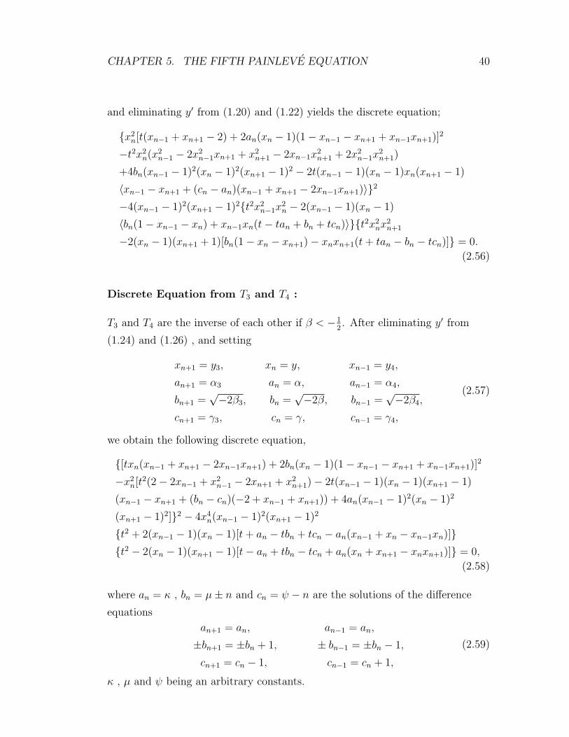
and eliminating y′ from (1.20) and (1.22) yields the discrete equation;
{x2n[t(xn−1 + xn+1 − 2) + 2an(xn − 1)(1− xn−1 − xn+1 + xn−1xn+1)]
2
−t2x2n(x2
n−1 − 2x2n−1xn+1 + x2
n+1 − 2xn−1x2n+1 + 2x2
n−1x2n+1)
+4bn(xn−1 − 1)2(xn − 1)2(xn+1 − 1)2 − 2t(xn−1 − 1)(xn − 1)xn(xn+1 − 1)
〈xn−1 − xn+1 + (cn − an)(xn−1 + xn+1 − 2xn−1xn+1)〉}2
−4(xn−1 − 1)2(xn+1 − 1)2{t2x2n−1x
2n − 2(xn−1 − 1)(xn − 1)
〈bn(1− xn−1 − xn) + xn−1xn(t− tan + bn + tcn)〉}{t2x2nx
2n+1
−2(xn − 1)(xn+1 + 1)[bn(1− xn − xn+1)− xnxn+1(t+ tan − bn − tcn)]} = 0.
(2.56)
Discrete Equation from T3 and T4 :
T3 and T4 are the inverse of each other if β < −12. After eliminating y′ from
(1.24) and (1.26) , and setting
xn+1 = y3, xn = y, xn−1 = y4,
an+1 = α3 an = α, an−1 = α4,
bn+1 =√−2β3, bn =
√−2β, bn−1 =
√−2β4,
cn+1 = γ3, cn = γ, cn−1 = γ4,
(2.57)
we obtain the following discrete equation,
{[txn(xn−1 + xn+1 − 2xn−1xn+1) + 2bn(xn − 1)(1− xn−1 − xn+1 + xn−1xn+1)]2
−x2n[t2(2− 2xn−1 + x2
n−1 − 2xn+1 + x2n+1)− 2t(xn−1 − 1)(xn − 1)(xn+1 − 1)
(xn−1 − xn+1 + (bn − cn)(−2 + xn−1 + xn+1)) + 4an(xn−1 − 1)2(xn − 1)2
(xn+1 − 1)2]}2 − 4x4n(xn−1 − 1)2(xn+1 − 1)2
{t2 + 2(xn−1 − 1)(xn − 1)[t+ an − tbn + tcn − an(xn−1 + xn − xn−1xn)]}{t2 − 2(xn − 1)(xn+1 − 1)[t− an + tbn − tcn + an(xn + xn+1 − xnxn+1)]} = 0,
(2.58)
where an = κ , bn = µ± n and cn = ψ − n are the solutions of the difference
equations
an+1 = an, an−1 = an,
±bn+1 = ±bn + 1, ± bn−1 = ±bn − 1,
cn+1 = cn − 1, cn−1 = cn + 1,
(2.59)
κ , µ and ψ being an arbitrary constants.

CHAPTER 5. THE FIFTH PAINLEVE EQUATION 41
Discrete Equation from T5 and T6 :
T5 and T6 are the inverse of each other if β < −12. After eliminating y′ from
(1.28) and (1.30) , and setting
xn+1 = y5, xn = y, xn−1 = y6,
an+1 = α5, an = α, an−1 = α6,
bn+1 =√−2β5, bn =
√−2β, bn−1 =
√−2β6,
cn+1 = γ5, cn = γ, cn−1 = γ6,
(2.60)
we obtain the following discrete equation,
{[2bn(xn − 1)(1− xn−1 − xn+1 + xn−1xn+1) + txn(−xn−1 − xn+1 + 2xn−1xn+1)]2
−x2n[t2(2− 2xn−1 + x2
n−1 − 2xn+1 + x2n+1) + 2t(xn−1 − 1)(xn − 1)(xn+1 − 1)
(xn+1 − xn−1 + (bn + cn)(xn−1 + xn+1 − 2)) + 4an(xn−1 − 1)2(xn − 1)2
(xn+1 − 1)2]}2 − 4(xn−1 − 1)2x4n(xn+1 − 1)2
{t2 + 2(xn−1 − 1)(xn − 1)[t+ an + tbn + tcn − an(xn−1 + xn − xn−1xn)]}{t2 − 2(xn − 1)(xn+1 − 1)[t− an − tbn − tcn + an(xn + x1+n − xnx1+n)]} = 0,
(2.61)
where an = κ , bn = µ∓ n and cn = ψ − n are the solutions of the difference
equations
an+1 = an, an−1 = an,
±bn+1 = ±bn − 1, ± bn−1 = ±bn + 1,
cn+1 = cn − 1, cn−1 = cn + 1,
(2.62)
κ , µ and ψ being an arbitrary constants.
Discrete Equation from T7 and T8 :
T7 and T8 are the inverse of each other if α > 12. After eliminating y′ from (1.32)
and (1.34) , and setting
xn+1 = y7, xn = y, xn−1 = y8,
an+1 =√
2α7, an =√
2α, an−1 =√
2α8,
bn+1 = β7, bn = β, bn−1 = β8,
cn+1 = γ7, cn = γ, cn−1 = γ8,
(2.63)
CHAPTER 5. THE FIFTH PAINLEVE EQUATION 42
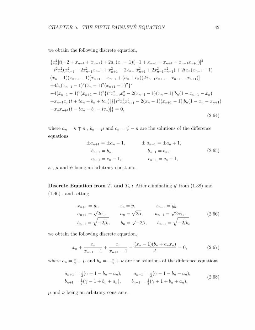
we obtain the following discrete equation,
{x2n[t(−2 + xn−1 + xn+1) + 2an(xn − 1)(−1 + xn−1 + xn+1 − xn−1xn+1)]
2
−t2x2n(x2
n−1 − 2x2n−1xn+1 + x2
n+1 − 2xn−1x2n+1 + 2x2
n−1x2n+1) + 2txn(xn−1 − 1)
(xn − 1)(xn+1 − 1)[xn+1 − xn−1 + (an + cn)(2xn−1xn+1 − xn−1 − xn+1)]
+4bn(xn−1 − 1)2(xn − 1)2(xn+1 − 1)2}2
−4(xn−1 − 1)2(xn+1 − 1)2{t2x2n−1x
2n − 2(xn−1 − 1)(xn − 1)[bn(1− xn−1 − xn)
+xn−1xn(t+ tan + bn + tcn)]}{t2x2nx
2n+1 − 2(xn − 1)(xn+1 − 1)[bn(1− xn − xn+1)
−xnxn+1(t− tan − bn − tcn)]} = 0,
(2.64)
where an = κ∓ n , bn = µ and cn = ψ − n are the solutions of the difference
equations
±an+1 = ±an − 1, ± an−1 = ±an + 1,
bn+1 = bn, bn−1 = bn,
cn+1 = cn − 1, cn−1 = cn + 1,
(2.65)
κ , µ and ψ being an arbitrary constants.
Discrete Equation from T1 and T5 : After eliminating y′ from (1.38) and
(1.46) , and setting
xn+1 = y1, xn = y, xn−1 = y5,
an+1 =√
2α1, an =√
2α, an−1 =√
2α5,
bn+1 =
√− ˜2β1, bn =
√−2β, bn−1 =
√− ˜2β5,
(2.66)
we obtain the following discrete equation,
xn +xn
xn−1 − 1+
xn
xn+1 − 1− (xn − 1)(bn + anxn)
t= 0, (2.67)
where an = n2
+ µ and bn = −n2
+ ν are the solutions of the difference equations
an+1 = 12(γ + 1− bn − an), an−1 = 1
2(γ − 1− bn − an),
bn+1 = 12(γ − 1 + bn + an), bn−1 = 1
2(γ + 1 + bn + an),
(2.68)
µ and ν being an arbitrary constants.

CHAPTER 5. THE FIFTH PAINLEVE EQUATION 43
Discrete Equation from T2 and T6 : After eliminating y′ from (1.40) and
(1.48) , and setting
xn+1 = y2, xn = y, xn−1 = y6,
an+1 =√
2α2, an =√
2α, an−1 =√
2α6,
bn+1 =
√− ˜2β2, bn =
√−2β, bn−1 =
√− ˜2β6,
(2.69)
we obtain the following discrete equation,
xn +xn
xn−1 − 1+
xn
xn+1 − 1+
(xn − 1)(bn + anxn)
t= 0, (2.70)
where an = n2
+ φ and bn = −n2
+ ϕ are the solutions of the difference equations
an+1 = 12(γ + 1 + bn + an), an−1 = 1
2(γ − 1 + bn + an),
bn+1 = 12(γ − 1− bn − an), bn−1 = 1
2(γ + 1− bn − an),
(2.71)
φ and ϕ being an arbitrary constants.
Discrete Equation from T3, T7 and T4,T8 :
After eliminating y′ between (1.42), (1.50)and between (1.44), (1.52), and
setting
xn+1 = y3, xn = y, xn−1 = y7, (2.72)
xn+1 = y4, xn = y, xn−1 = y8, (2.73)
we obtain the following discrete equation
2xn
(1 +
1
xn−1 − 1+
1
xn+1 − 1
)= 0. (2.74)

Chapter 6
The Sixth Painleve Equation
The sixth Painleve equation
d2y
dt2=
1
2
(1
y+
1
y − 1+
1
y − t
)(dy
dt
)2
−(
1
t+
1
t− 1+
1
y − t
)dy
dt
+y(y − 1)(y − t)
t2(t− 1)2
(α+ β
t
y2+ γ
t− 1
(y − 1)2+ δ
t(t− 1)
(y − t)2
),
(0.1)
can be obtained as the compatibility condition of the following linear system of
equations [22]
Yz(z, t) = A(z, t)Y (z, t), Yt(z, t) = B(z, t)Y (z, t), (0.2)
where
A(z, t) =A0
z+
A1
z − 1+
At
z − t=
(a11(z, t) a12(z, t)
a21(z, t) a22(z, t)
),
A0 =
(u0 + θ0 −w0u0
w0−1(u0 + θ0) −u0
), A1 =
(u1 + θ1 −w1u1
w1−1(u1 + θ1) −u1
),
At =
(ut + θt −wtut
wt−1(ut + θt) −ut
), B(z, t) = −At
1
z − t.
(0.3)
44

CHAPTER 6. THE SIXTH PAINLEVE EQUATION 45
Schlesinger transformations and the closed form of the Backlund transformations
derived by Mugan and Sakka [31]. Setting,
A∞ = −(A0 + A1 + At) =
(κ1 0
0 κ2
),
κ1 + κ2 = −(θ0 + θ1 + θt), κ1 − κ2 = θ∞,
a12(z, t) = −w0u0
z− w1u1
z − 1− wtut
z − t=
k(z − y)
z(z − 1)(z − t),
u = a11(y) =u0 + θ0
y+u1 + θ1
y − 1+ut + θt
y − t,
u = −a22(y) = u− θ0
y− θ1
y − 1− θt
y − t.
(0.4)
Thenu0 + u1 + ut = κ2, w0u0 + w1u1 + wtut = 0,u0 + θ0
w0
+u1 + θ1
w1
+ut + θt
wt
= 0,
(t+ 1)w0u0 + tw1u1 + wtut = k, tw0u0 = k(t)y,
(0.5)
which are solved as,
w0 =ky
tu0
, w1 = − k(y − 1)
u1(t− 1), wt =
k(y − t)
t(t− 1)ut
,
u0 =y
tθ∞{y(y − 1)(y − t)u2 + [θ1(y − t) + tθt(y − 1)− 2κ2(y − 1)(y − t)]u
+κ22(y − t− 1)− κ2(θ1 + tθt)},
u1 = − y − 1
(t− 1)θ∞{y(y − 1)(y − t)u2 + [(θ1 + θ∞)(y − t) + tθt(y − 1)
−2κ2(y − 1)(y − t)]u+ κ22(y − t)− κ2(θ1 + tθt)− κ1κ2},
ut =y − t
t(t− 1)θ∞{y(y − 1)(y − t)u2 + [θ1(y − t) + t(θt + θ∞)(y − 1)−
2κ2(y − 1)(y − t)]u+ κ22(y − 1)− κ2(θ1 + tθt)− tκ1κ2}.
(0.6)
The equation Yzt = Ytz implies
dy
dt=y(y − 1)(y − t)
t(t− 1)
(2u− θ0
y− θ1
y − 1− θt − 1
y − t
),
du
dt=
1
t(t− 1){[−3y2 + 2(1 + t)y − t]u2
+[(2y − 1− t)θ0 + (2y − t)θ1 + (2y − 1)(θt − 1)]u− κ1(κ2 + 1)},1
k
dk
dt= (θ∞ − 1)
y − t
t(t− 1).
(0.7)

CHAPTER 6. THE SIXTH PAINLEVE EQUATION 46
Thus y satisfies the sixth Painleve equation (0.1), with the parameters
α =1
2(θ∞ − 1)2, β = −1
2θ20, γ =
1
2θ21, δ =
1
2(1− θ2
t ). (0.8)
6.1 Backlund Transformations
Let R(z, t) be the transformation matrix which transforms the solution of the
linear problem (0.2) as;
Y ′(z, t) = R(z, t)Y (z, t), (1.9)
but leaves the monodromy data associated with Y (z) the same. Let u′i, w′i, θ
′i =
θi+λi be the transformed quantities of ui, wi, θi, i = 0, 1, t,∞. The consistency
condition of the monodromy data is invariant under the transformation if λ1 +
λ0 = k, λ1 − λ0 = l,
λ∞ + λt = m, λ∞ − λt = n, where k, l,m, n are either odd or even integers. It
is enough to consider the following three cases;
a :
θ′0 = θ0 + λ0
θ′1 = θ1
θ′t = θt
θ′∞ = θ∞ + λ∞,
b :
θ′0 = θ0
θ′1 = θ1 + λ1
θ′t = θt
θ′∞ = θ∞ + λ∞,
c :
θ′0 = θ0
θ′1 = θ1
θ′t = θt + λt
θ′∞ = θ∞ + λ∞,
(1.10)
All possible Schlesinger transformations admitted by the linear problem (0.2)
may be generated by the following transformation matrices :θ′0 = θ0 + 1
θ′1 = θ1
θ′t = θt
θ′∞ = θ∞ + 1,
R(1)(z, t) =
(0 0
0 1
)z +
(1 −w0
−r1 w0r1
),
(1.11)

CHAPTER 6. THE SIXTH PAINLEVE EQUATION 47
θ′0 = θ0 − 1
θ′1 = θ1
θ′t = θt
θ′∞ = θ∞ − 1,
R(2)(z, t) =
(1 0
0 0
)+
(u0+θ0
u0w0r2 −r2
−u0+θ0
u0w01
)1z,
(1.12)θ′0 = θ0 − 1
θ′1 = θ1
θ′t = θt
θ′∞ = θ∞ + 1,
R(3)(z, t) =
(0 0
0 1
)+
(1 − u0w0
u0+θ0
−r1 u0w0
u0+θ0r1
)1z,
(1.13)θ′0 = θ0 + 1
θ′1 = θ1
θ′t = θt
θ′∞ = θ∞ − 1,
R(4)(z, t) =
(1 0
0 0
)z +
(r2
w0−r2
− 1w0
1
),
(1.14)θ′0 = θ0
θ′1 = θ1 + 1
θ′t = θt
θ′∞ = θ∞ + 1,
R(5)(z, t) =
(0 0
0 1
)(z − 1) +
(1 −w1
−r1 w1r1
),
(1.15)θ′0 = θ0
θ′1 = θ1 − 1
θ′t = θt
θ′∞ = θ∞ − 1,
R(6)(z, t) =
(1 0
0 0
)+
(u1+θ1
u0w0r2 −r2
−u1+θ1
u1w11
)1
z−1,
(1.16)θ′0 = θ0
θ′1 = θ1 − 1
θ′t = θt
θ′∞ = θ∞ + 1,
R(7)(z, t) =
(0 0
0 1
)+
(1 − u1w1
u1+θ1
−r1 u1w1
u1+θ1r1
)1
z−1,
(1.17)

CHAPTER 6. THE SIXTH PAINLEVE EQUATION 48
θ′0 = θ0
θ′1 = θ1 + 1
θ′t = θt
θ′∞ = θ∞ − 1,
R(8)(z, t) =
(1 0
0 0
)(z − 1) +
(r2
w1−r2
− 1w1
1
),
(1.18)θ′0 = θ0
θ′1 = θ1
θ′t = θt + 1
θ′∞ = θ∞ + 1,
R(9)(z, t) =
(0 0
0 1
)(z − t) +
(1 −wt
−r1 wtr1
),
(1.19)θ′0 = θ0
θ′1 = θ1
θ′t = θt − 1
θ′∞ = θ∞ − 1,
R(10)(z, t) =
(1 0
0 0
)+
(ut+θt
utwtr2 −r2
−ut+θt
utwt1
)1
z−t,
(1.20)θ′0 = θ0
θ′1 = θ1
θ′t = θt − 1
θ′∞ = θ∞ + 1,
R(11)(z, t) =
(0 0
0 1
)+
(1 − utwt
ut+θt
−r1 utwt
ut+θtr1
)1
z−t,
(1.21)θ′0 = θ0
θ′1 = θ1
θ′t = θt + 1
θ′∞ = θ∞ − 1,
R(12)(z, t) =
(1 0
0 0
)(z − t) +
(r2
wt−r2
− 1wt
1
),
(1.22)
where
r1 = − 1
1 + θ∞
(u1 + θ1
w1
+ut + θt
wt
t
), r2 =
1
1− θ∞(w1u1 + twtut), (1.23)
and ui, wi, i = 0, 1, t are given in (0.6). The transformation matrices
R(k)(z, t), k = 1, 2, ..., 12 are sufficient to obtain the transformation matrix
R(z, t) which shifts the exponents θ0, θ1, θt, θ∞ to θ′0, θ′1, θ
′t, θ
′∞ with any inte-
ger differences. If,
Y ′(z, t;u′0, u′1, u
′t, w
′0, w
′1, w
′t, θ
′0, θ1, θ
′t, θ
′∞) = R(j)(z, t;u0, ..., θ∞)Y (z, t;u0, ..., θ∞),
(1.24)
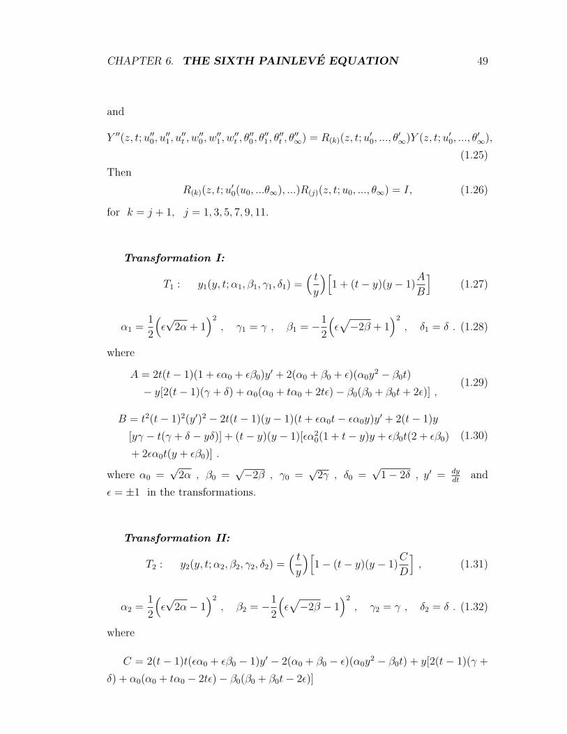
CHAPTER 6. THE SIXTH PAINLEVE EQUATION 49
and
Y ′′(z, t;u′′0, u′′1, u
′′t , w
′′0 , w
′′1 , w
′′t , θ
′′0 , θ
′′1 , θ
′′t , θ
′′∞) = R(k)(z, t;u
′0, ..., θ
′∞)Y (z, t;u′0, ..., θ
′∞),
(1.25)
Then
R(k)(z, t;u′0(u0, ...θ∞), ...)R(j)(z, t;u0, ..., θ∞) = I, (1.26)
for k = j + 1, j = 1, 3, 5, 7, 9, 11.
Transformation I:
T1 : y1(y, t;α1, β1, γ1, δ1) =( ty
)[1 + (t− y)(y − 1)
A
B
](1.27)
α1 =1
2
(ε√
2α+ 1)2
, γ1 = γ , β1 = −1
2
(ε√−2β + 1
)2
, δ1 = δ . (1.28)
where
A = 2t(t− 1)(1 + εα0 + εβ0)y′ + 2(α0 + β0 + ε)(α0y
2 − β0t)
− y[2(t− 1)(γ + δ) + α0(α0 + tα0 + 2tε)− β0(β0 + β0t+ 2ε)] ,(1.29)
B = t2(t− 1)2(y′)2 − 2t(t− 1)(y − 1)(t+ εα0t− εα0y)y′ + 2(t− 1)y
[yγ − t(γ + δ − yδ)] + (t− y)(y − 1)[εα20(1 + t− y)y + εβ0t(2 + εβ0)
+ 2εα0t(y + εβ0)] .
(1.30)
where α0 =√
2α , β0 =√−2β , γ0 =
√2γ , δ0 =
√1− 2δ , y′ = dy
dtand
ε = ±1 in the transformations.
Transformation II:
T2 : y2(y, t;α2, β2, γ2, δ2) =( ty
)[1− (t− y)(y − 1)
C
D
], (1.31)
α2 =1
2
(ε√
2α− 1)2
, β2 = −1
2
(ε√−2β − 1
)2
, γ2 = γ , δ2 = δ . (1.32)
where
C = 2(t− 1)t(εα0 + εβ0 − 1)y′ − 2(α0 + β0 − ε)(α0y2 − β0t) + y[2(t− 1)(γ +
δ) + α0(α0 + tα0 − 2tε)− β0(β0 + β0t− 2ε)]

CHAPTER 6. THE SIXTH PAINLEVE EQUATION 50
D = (t− 1)2t2(y′)2− 2(t− 1)t(y− 1)(t− εα0t+ εα0y)y′ + 2(t− 1)y[yγ− t(γ +
δ − yδ)] + (t− y)(y − 1)[εα20(1 + t− y)y + β0t(β0 − 2ε)− 2α0t(εy − β0)]
Transformation III:
T3 : y3(y, t;α3, β3, γ3, δ3) =( ty
)[1 + (t− y)(y − 1)
E
F
](1.33)
α3 =1
2
(ε√
2α+ 1)2
, β3 = −1
2
(ε√−2β − 1
)2
, γ3 = γ , δ3 = δ . (1.34)
where
E = 2(t− 1)t(εα0 − εβ0 + 1)y′ + 2(α0 − β0 + ε)(α0y2 + β0t)− y[2(t− 1)(γ +
δ) + α0(α0 + α0t+ 2εt)− β0(β0 + β0t− 2ε)]
F = (t− 1)2t2(y′)2− 2(t− 1)t(y− 1)(t+ εα0t− εα0y)y′ + 2(t− 1)y[yγ − t(γ +
δ − yδ)] + (t− y)(y − 1)[εα20y(1 + t− y) + 2α0t(εy − β0) + β0t(β0 − 2ε)]
Transformation IV:
T4 : y4(y, t;α4, β4, γ4, δ4) =( ty
)[1− (t− y)(y − 1)
G
H
](1.35)
α4 =1
2
(ε√
2α− 1)2
, β4 = −1
2
(ε√−2β + 1
)2
, γ4 = γ , δ4 = δ (1.36)
where
G = 2(t− 1)t(εα0 − εβ0 − 1)y′ − 2(α0 − β0 − ε)(α0y2 + β0t)
+ y[2(t− 1)(γ + δ) + α0(α0 + α0t− 2εt)− β0(β0 + β0t+ 2ε)]
H = (t− 1)2t2(y′)2 + 2(t− 1)t(y − 1)(εα0t− εα0y − t)y′
+ 2(t− 1)y[yγ − t(γ + δ− yδ)] + (t− y)(y− 1)[εα20y(1 + t− y) + β0t(2ε+ β0)−
2α0t(εy + β0)]
Transformation V:
T5 : y5(y, t;α5, β5, γ5, δ5) =( y − t
y − 1
)[1 + (t− 1)y
I
J
](1.37)

CHAPTER 6. THE SIXTH PAINLEVE EQUATION 51
α5 =1
2
(ε√
2α+ 1)2
, β5 = β , γ5 =1
2
(ε√
2γ + 1)2
, δ5 = δ (1.38)
where
I = 2(t − 1)t(εα0 + εγ0 + 1)y′ + 2α0(α0 + γ0 + ε)y2 − y[2(α0 + γ0)(ε + α0 +
γ0) + εt(2εδ + 2α0 + α20 − 2εβ − γ2
0)] + t[(α0 + γ0)2 + 2(δ + εα0 + εγ0)− 2β]
J = (t−1)2t2(y′)2−2(t−1)ty(t+ εα0t− εα0y−1)y′+2(t−1)t(y−1)yδ+(t−y)[εα2
0y(t−y−1)(y−1)−2t(y−1)β+2εα0(t−1)y(y−εγ0−1)−γ0y(t−1)(2ε+γ0)]
Transformation VI:
T6 : y6(y, t;α6, β6, γ6, δ6) =( y − t
y − 1
)(1− y
K
L
)(1.39)
α6 =1
2
(ε√
2α− 1)2
, β6 = β , γ6 =1
2
(ε√
2γ − 1)2
, δ6 = δ . (1.40)
where
K = 2(t− 1)2t(εα0 + εγ0 − 1)y′ + εα20(t− 1)(t− 2y)(y− 1) + 2εα0{(t− y)(y−
1)(1− t+ 4tβ1) + εγ0[t2(3− 4y) + t(1 + y(3y − 2)) + y(y − 2)]}+ (t− 1){2t(y −
1)(δ − β) + 2εγ0(t− y)− εγ20 [t+ (t− 2)y]}
L = (t− 1)2t2(y′)2 + 2(t− 1)ty(1− t+ εα0t− εα0y)y′ + 2(t− 1)t(y − 1)yδ +
(t− y){εα20y(t− y − 1)(y − 1)− 2t(y − 1)β − γ0(t− 1)y(γ0 − 2ε) + 2εα0y[t+ y −
ty − 1 + 4β1t(y − 1) + εγ0(1 + 3t− 4ty)]}
Transformation VII:
T7 : y7(y, t;α7, β7, γ7, δ7) =( y − t
y − 1
)[1 + y(t− 1)
M
N
](1.41)
α7 =1
2
(ε√
2α+ 1)2
, β7 = β , γ7 =1
2
(ε√
2γ − 1)2
, δ7 = δ . (1.42)
where
M = 2(t − 1)t(εγ0 − εα0 − 1)y′ + (y − 1)[2εα0(t − y) + εα20(t − 2y) + 2t(δ −
β)] + 2εγ0{t− y + εα0[t+ y(y − 2)]} − εγ20 [t+ y(t− 2)]

CHAPTER 6. THE SIXTH PAINLEVE EQUATION 52
N = (t−1)2t2(y′)2−2(t−1)ty(t+ εα0t− εα0y−1)y′+2(t−1)t(y−1)yδ+(t−y)[εα2
0y(t−y−1)(y−1)−2t(y−1)β−γ0(t−1)y(γ0−2ε)+2εα0(t−1)y(y+εγ0−1)]
Transformation VIII:
T8 : y8(y, t;α8, β8, γ8, δ8) =( y − t
y − 1
)[1− y(t− 1)
P
R
](1.43)
α8 =1
2
(ε√
2α− 1)2
, β8 = β , γ8 =1
2
(ε√
2γ + 1)2
, δ8 = δ . (1.44)
where
P = 2(t− 1)t(εγ0 − εα0 + 1)y′ + 2t(y − 1)(β − δ) + α0(y − 1)[2ε(t− y)− (t−2y)α0]− 2εγ0{y − t+ εα0[t+ (y − 2)y]}+ εγ2
0 [t+ (t− 2)y]
R = (t− 1)2t2(y′)2 + 2(t− 1)ty(1− t+ εα0t− εα0y)y′ + 2t(y − 1)(yβ − tβ −
yδ+tyδ)+(t−y)y[εα20(t−y−1)(y−1)−γ0(t−1)(2ε+γ0)+2εα0(t−1)(1−y+εγ0)]
Transformation IX:
T9 : y9(y, t;α9, β9, γ9, δ9) = t2(y − 1
y − t
)[1− (t− 1)y
S
T
](1.45)
α9 =1
2
(ε√
2α+ 1)2
, β9 = β , γ9 = γ , δ9 =1
2− 1
2
(ε√
1− 2δ + 1)2
(1.46)
where
S = 2(t − 1)t(εα0 + εδ0 + 1)y′ + 2α0y2(ε + α0 + δ0) + y[(1 + εδ0)
2 − 2t(α0 +
δ0)(2ε+α0 + δ0)− 2(t− γ)− εα20 + 2β] + t[1− 2β + 2(εα0− γ + εδ0) + (α0 + δ0)
2]
T = (t− 1)2t2(y′)2 + 2εα0(t− 1)ty(y− 1)y′ + εα20y
3(y− 2)− y2{(t− 1)[t(α0 +
δ0)2 − 2(γ − εα0t− εδ0t) + t]− εα2
0 − 2tβ}+ ty{(t− 1)[(α0 + δ0)2 − 2(γ − εα0 −
εδ0) + 1]− 2(t+ 1)β}+ 2t2β
Transformation X:
T10 : y10(y, t;α10, β10, γ10, δ10) = t(y − 1
y − t
)[1 + (t− 1)y
U
V
](1.47)

CHAPTER 6. THE SIXTH PAINLEVE EQUATION 53
α10 =1
2
(ε√
2α−1)2
, β10 = β , γ10 = γ , δ10 =1
2− 1
2
(ε√
1− 2δ−1)2
. (1.48)
where
U = 2(t − 1)t(εα0 + εδ0 − 1)y′ − 2α0y2(α0 + δ0 − ε) + y[2t(εα0 + εδ0 − 1)2 −
(εδ0 − 1)2 − 2(β + γ) + εα20] + t[2(β + γ + εα0 + εδ0)− (α0 + δ0)
2 − 1]
V = (t− 1)2t2(y′)2 − 2εα0(t− 1)ty(y − 1)y′ + εα20y
3(y − 2)
− y2{(t− 1)[t(α0 + δ0)2− 2(γ + tεα0 + tεδ0) + t]− εα2
0− 2tβ}+ ty{(t− 1)[(α0 +
δ0)2 − 2(γ + εα0 + εδ0) + 1]− 2(1 + t)β}+ 2t2β
Transformation XI:
T11 : y11(y, t;α11, β11, γ11, δ11) = t(y − 1
y − t
)[1− (t− 1)y
Z
X
](1.49)
α11 =1
2
(ε√
2α+1)2
, β11 = β , γ11 = γ , δ11 =1
2− 1
2
(ε√
1− 2δ−1)2
(1.50)
where
Z = 2(t − 1)t(εα0 − εδ0 + 1)y′ + 2y2α0(α0 − δ0 + ε) − y[2t(εα0 − εδ0 + 1)2 −(εδ0 − 1)2 − 2γ − 2β + εα2
0] + t[(α0 − δ0)2 − 2β − 2(γ − εα0 + εδ0) + 1]
X = (t− 1)2t2(y′)2 + 2εα0(t− 1)ty(y− 1)y′ + εα20y
3(y− 2)− y2{(t− 1)[t(α0−δ0)
2 − 2(γ − εα0t+ εδ0t) + t]− εα20 − 2tβ}+ ty{(t− 1)[(α0 − δ0)
2 − 2(γ − εα0 +
εδ0) + 1]− 2(t+ 1)β}+ 2t2β
Transformation XII:
T12 : y12(y, t;α12, β12, γ12, δ12) = t(y − 1
y − t
)[1 + (t− 1)y
ζ
η
](1.51)
α12 =1
2
(ε√
2α−1)2
, β12 = β , γ12 = γ , δ12 =1
2− 1
2
(ε√
1− 2δ+1)2
. (1.52)
where
ζ = 2(t − 1)t(εα0 − εδ0 − 1)y′ − 2α0y2(α0 − δ0 − ε) + y[2t(εα0 − εδ0 − 1)2 −
(εδ0 + 1)2 − 2(β + γ) + εα20]− t[(α0 − δ0)
2 − 2(β + γ + εα0 − εδ0) + 1]

CHAPTER 6. THE SIXTH PAINLEVE EQUATION 54
η = (t− 1)2t2(y′)2 − 2εα0(t− 1)ty(y − 1)y′ + εα20y
3(y − 2)− y2{(t− 1)[t(α0 −δ0)
2 − 2(γ + εα0t− εδ0t) + t]− 2tβ − εα20}
+ ty{(t− 1)[(α0 − δ0)2 − 2(γ + εα0 − εδ0) + 1]− 2(t+ 1)β}+ 2t2β
There are sixteen known Backlund transformations [15] in the compact form
as follows:
y = y − σy(y − 1)(y − t)
t(t− 1)y′ + y2(η2 + η3 + η4 − 1)− y(tη2 + tη3 + η2 + η4 − 1) + tη2
(1.53)
where η12 = 2α, η2
2 = −2β, η32 = 2γ, η4
2 = 1− 2δ and σ = −1 +∑4
k=1 ηk.
The parameters change
α =η2
1
2, β = − η
22
2, γ =
η23
2, δ =
1− η24
2(1.54)
where ηj = 12
+ ηj − 12
∑4k=1 ηk.
We use the notations a, b, c, d for simplicity, which are a =√
2α, b =√−2β,
c =√
2γ, d =√
1− 2δ.
T1 : y1 = y− (a+ b+ c+ d− 1)y(y − 1)(y − t)
t(t− 1)y′ + y2(b+ c+ d− 1)− y(tb+ tc+ b+ d− 1) + tb(1.55)
α1 =( 12+a− 1
2(a+b+c+d))2
2, β1 = − ( 1
2+b− 1
2(a+b+c+d))2
2,
γ1 =( 12+c− 1
2(a+b+c+d))2
2, δ1 =
1−( 12+d− 1
2(a+b+c+d))2
2
(1.56)

CHAPTER 6. THE SIXTH PAINLEVE EQUATION 55
T2 : y2 = y− (a+ b+ c− d− 1)y(y − 1)(y − t)
t(t− 1)y′ + y2(b+ c− d− 1)− y(tb+ tc+ b− d− 1) + tb(1.57)
α2 =( 12+a− 1
2(a+b+c−d))2
2, β2 = − ( 1
2+b− 1
2(a+b+c−d))2
2,
γ2 =( 12+c− 1
2(a+b+c−d))2
2, δ2 =
1−( 12−d− 1
2(a+b+c−d))2
2
(1.58)
T3 : y3 = y− (a+ b− c+ d− 1)y(y − 1)(y − t)
t(t− 1)y′ + y2(b− c+ d− 1)− y(tb− tc+ b+ d− 1) + tb(1.59)
α3 =( 12+a− 1
2(a+b−c+d))2
2, β3 = − ( 1
2+b− 1
2(a+b−c+d))2
2,
γ3 =( 12−c− 1
2(a+b−c+d))2
2, δ3 =
1−( 12+d− 1
2(a+b−c+d))2
2
(1.60)
T4 : y4 = y − (a− b+ c+ d− 1)y(y − 1)(y − t)
t(t− 1)y′ + y2(−b+ c+ d− 1)− y(−tb+ tc− b+ d− 1)− tb(1.61)
α4 =( 12+a− 1
2(a−b+c+d))2
2, β4 = − ( 1
2−b− 1
2(a−b+c+d))2
2,
γ4 =( 12+c− 1
2(a−b+c+d))2
2, δ4 =
1−( 12+d− 1
2(a−b+c+d))2
2
(1.62)
T5 : y5 = y− (a+ b− c− d− 1)y(y − 1)(y − t)
t(t− 1)y′ + y2(b− c− d− 1)− y(tb− tc+ b− d− 1) + tb(1.63)
α5 =( 12+a− 1
2(a+b−c−d))2
2, β5 = − ( 1
2+b− 1
2(a+b−c−d))2
2,
γ5 =( 12−c− 1
2(a+b−c−d))2
2, δ5 =
1−( 12−d− 1
2(a+b−c∗d))2
2
(1.64)

CHAPTER 6. THE SIXTH PAINLEVE EQUATION 56
T6 : y6 = y − (a− b+ c− d− 1)y(y − 1)(y − t)
t(t− 1)y′ + y2(−b+ c− d− 1)− y(−tb+ tc− b− d− 1)− tb(1.65)
α6 =( 12+a− 1
2(a−b+c−d))2
2, β6 = − ( 1
2−b− 1
2(a−b+c−d))2
2,
γ6 =( 12+c− 1
2(a−b+c−d))2
2, δ6 =
1−( 12−d− 1
2(a−b+c−d))2
2
(1.66)
T7 : y7 = y − (a− b− c+ d− 1)y(y − 1)(y − t)
t(t− 1)y′ + y2(−b− c+ d− 1)− y(−tb− tc− b+ d− 1)− tb(1.67)
α7 =( 12+a− 1
2(a−b−c+d))2
2, β7 = − ( 1
2−b− 1
2(a−b−c+d))2
2,
γ7 =( 12−c− 1
2(a−b−c+d))2
2, δ7 =
1−( 12+d− 1
2(a−b−c+d))2
2
(1.68)
T8 : y8 = y − (a− b− c− d− 1)y(y − 1)(y − t)
t(t− 1)y′ + y2(−b− c− d− 1)− y(−tb− tc− b− d− 1)− tb(1.69)
α8 =( 12+a− 1
2(a−b−c−d))2
2, β8 = − ( 1
2−b− 1
2(a−b−c−d))2
2,
γ8 =( 12−c− 1
2(a−b−c−d))2
2, δ8 =
1−( 12−d− 1
2(a−b−c−d))2
2
(1.70)
T9 : y9 = y− (−a+ b+ c+ d− 1)y(y − 1)(y − t)
t(t− 1)y′ + y2(b+ c+ d− 1)− y(tb+ tc+ b+ d− 1) + tb(1.71)

CHAPTER 6. THE SIXTH PAINLEVE EQUATION 57
α9 =( 12−a− 1
2(−a+b+c+d))2
2, β9 = − ( 1
2+b− 1
2(−a+b+c+d))2
2,
γ9 =( 12+c− 1
2(−a+b+c+d))2
2, δ9 =
1−( 12+d− 1
2(−a+b+c+d))2
2
(1.72)
T10 : y10 = y − (−a+ b+ c− d− 1)y(y − 1)(y − t)
t(t− 1)y′ + y2(b+ c− d− 1)− y(tb+ tc+ b− d− 1) + tb(1.73)
α10 =( 12−a− 1
2(−a+b+c−d))2
2, β10 = − ( 1
2+b− 1
2(−a+b+c−d))2
2,
γ10 =( 12+c− 1
2(−a+b+c−d))2
2, δ10 =
1−( 12−d− 1
2(−a+b+c−d))2
2
(1.74)
T11 : y11 = y − (−a+ b− c+ d− 1)y(y − 1)(y − t)
t(t− 1)y′ + y2(b− c+ d− 1)− y(tb− tc+ b+ d− 1) + tb(1.75)
α11 =( 12−a− 1
2(−a+b−c+d))2
2, β11 = − ( 1
2+b− 1
2(−a+b−c+d))2
2,
γ11 =( 12−c− 1
2(−a+b−c+d))2
2, δ11 =
1−( 12+d− 1
2(−a+b−c+d))2
2
(1.76)
T12 : y12 = y − (−a− b+ c+ d− 1)y(y − 1)(y − t)
t(t− 1)y′ + y2(−b+ c+ d− 1)− y(−tb+ tc− b+ d− 1)− tb(1.77)
α12 =( 12−a− 1
2(−a−b+c+d))2
2, β12 = − ( 1
2−b− 1
2(−a−b+c+d))2
2,
γ12 =( 12+c− 1
2(−a−b+c+d))2
2, δ12 =
1−( 12+d− 1
2(−a−b+c+d))2
2
(1.78)

CHAPTER 6. THE SIXTH PAINLEVE EQUATION 58
T13 : y13 = y − (−a+ b− c− d− 1)y(y − 1)(y − t)
t(t− 1)y′ + y2(b− c− d− 1)− y(tb− tc+ b− d− 1) + tb(1.79)
α13 =( 12−a− 1
2(−a+b−c−d))2
2, β13 = − ( 1
2+b− 1
2(−a+b−c−d))2
2,
γ13 =( 12−c− 1
2(−a+b−c−d))2
2, δ13 =
1−( 12−d− 1
2(−a+b−c−d))2
2
(1.80)
T14 : y14 = y − (−a− b+ c− d− 1)y(y − 1)(y − t)
t(t− 1)y′ + y2(−b+ c− d− 1)− y(−tb+ tc− b− d− 1)− tb(1.81)
α14 =( 12−a− 1
2(−a−b+c−d))2
2, β14 = − ( 1
2−b− 1
2(−a−b+c−d))2
2,
γ14 =( 12+c− 1
2(−a−b+c−d))2
2, δ14 =
1−( 12−d− 1
2(−a−b+c−d))2
2
(1.82)
T15 : y15 = y − (−a− b− c+ d− 1)y(y − 1)(y − t)
t(t− 1)y′ + y2(−b− c+ d− 1)− y(−tb− tc− b+ d− 1)− tb(1.83)
α15 =( 12−a− 1
2(−a−b−c+d))2
2, β15 = − ( 1
2−b− 1
2(−a−b−c+d))2
2,
γ15 =( 12−c− 1
2(−a−b−c+d))2
2, δ15 =
1−( 12+d− 1
2(−a−b−c+d))2
2
(1.84)
T16 : y16 = y − (−a− b− c− d− 1)y(y − 1)(y − t)
t(t− 1)y′ + y2(−b− c− d− 1)− y(−tb− tc− b− d− 1)− tb(1.85)

CHAPTER 6. THE SIXTH PAINLEVE EQUATION 59
α16 =( 12−a+ 1
2(a+b+c+d))2
2, β16 = − ( 1
2−b+ 1
2(a+b+c+d))2
2,
γ16 =( 12−c+ 1
2(a+b+c+d))2
2, δ16 =
1−( 12−d+ 1
2(a+b+c+d))2
2
(1.86)
6.2 Discrete Equations
The Backlund transformations that are inverse of each other, i.e. Ti ◦ Tj = I ,
j = i+ 1 , i = 1, 3, 5, 7 will be used to get the discrete equations.
Discrete Equation from T1 and T2 :
T1 and T2 are the inverse of each other if α > 12
and β < −12. Setting
an+1 =√
2α1, an =√
2α, an−1 =√
2α2, bn+1 =√−2β1, bn =
√−2β,
bn−1 =√−2β2, cn+1 = γ1, cn = γ, cn−1 = γ2, dn+1 = δ1, dn = δ, dn−1 = δ2 in the
parameter relations yield the difference equations
±an+1 = ±an + 1, ± an−1 = ±an − 1,
±bn+1 = ±bn + 1, ± bn−1 = ±bn − 1,
cn+1 = cn, cn−1 = cn,
dn+1 = dn, dn−1 = dn,
(2.87)
which have the solutions an = κ± n, bn = µ± n, cn = ψ and dn = φ, where
κ, µ, φ and ψ are arbitrary constants. Hence, setting
xn+1 = y1, xn = y, xn−1 = y2 (2.88)
and eliminating y′ from (1.27) and (1.31) yields the discrete equation;
B1(xnxn+1 − t)− A1x2n(xn−1xn − t)− 4xn(xn − t)(xn − 1)[2t2bn
+txn−1xn(an − bn − 2) + txnxn+1(an − bn) + 2xn−1x2nxn+1(1− an)] = 0
(2.89)
where,

CHAPTER 6. THE SIXTH PAINLEVE EQUATION 60
A1 = 4{t(an + bn)2(t− xn)(xn − 1)(t− xn+1)(xn+1 − 1)
+ (t− 1)(t− xnxn+1)[t(tc2n − d2
n) + t(d2n − c2n)(xn + xn+1) + xnxn+1(c
2n − td2
n)]}1/2,
B1 = 4x2n{t(an + bn − 2)2(t− xn−1)(xn−1 − 1)(t− xn)(xn − 1)
+ (t− 1)(t− xn−1xn)[t(tc2n − d2n) + t(d2
n − c2n)(xn−1 + xn) + xn−1xn(c2n − td2n)]}1/2.
Discrete Equation from T3 and T4 :
T3 and T4 are the inverse of each other if α > 12
and β < −12. After eliminating
y′ from (1.33) and (1.35) , and setting
xn+1 = y3, xn = y, xn−1 = y4,
an+1 =√
2α3, an =√
2α, an−1 =√
2α4,
bn+1 =√−2β3, bn =
√−2β, bn−1 =
√−2β4,
cn+1 = γ3, cn = γ, cn−1 = γ4,
dn+1 = δ3, dn = δ, dn−1 = δ4,
(2.90)
we obtain the following discrete equation,
A2(xn−1xn − t)−B2x2n(xnxn+1 − t)− 4xn(xn − t)(xn − 1)[2t2bn
+txn−1xn(2− an − bn)− txnxn+1(an + bn) + 2xn−1x2nxn+1(an − 1)] = 0
(2.91)
where,
A2 = 4x2n{t(an − bn)2(t− xn)(xn − 1)(t− xn+1)(xn+1 − 1)
+ (t− 1)(t− xnxn+1)[t(tc2n − d2
n) + t(d2n − c2n)(xn+1 + xn) + xn+1xn(c2n − td2
n)]}1/2,
B2 = 4{t(an − bn − 2)2(t− xn−1)(xn−1 − 1)(t− xn)(xn − 1)
+ (t− 1)(t− xn−1xn)[t(tc2n − d2n) + t(d2
n − c2n)(xn−1 + xn) + xn−1xn(c2n − td2n)]}1/2.
where an = κ ± n ,bn = µ ∓ n ,cn = ψ and dn = φ are the solutions of the
difference equations
±an+1 = ±an + 1 ± an−1 = ±an − 1,
±bn+1 = ±bn − 1 ± bn−1 = ±bn + 1,
cn+1 = cn cn−1 = cn,
dn+1 = dn dn−1 = dn.
(2.92)

CHAPTER 6. THE SIXTH PAINLEVE EQUATION 61
κ , µ ,ψ and φ being arbitrary constants.
Discrete Equation from T5 and T6 :
T5 and T6 are the inverse of each other if α > 12
and γ > 12. After eliminating y′
from (1.37) and (1.39) , and setting
xn+1 = y5, xn = y, xn−1 = y6,
an+1 =√
2α5, an =√
2α, an−1 =√
2α6,
bn+1 = β5, bn = β, bn−1 = β6,
cn+1 =√
2γ5, cn =√
2γ, cn−1 =√
2γ6,
dn+1 = δ5, dn = δ, dn−1 = δ6,
(2.93)
we obtain the following discrete equation,
A3[(xn − t)(xn − 1)2 − xn−1(xn − 1)3] +B3[xn(xn+1 − 1)− xn+1 + t]
−4xn(xn − t)(xn − 1){(an + tan + cn − tcn)[2(xn − t)
−(xn − 1)(xn−1 + xn+1)] + 2(t+ 1)xn(xn−1 − 1)− 2anxn(xn−1 + xn+1)
+2(t+ t2an − txn−1 − xn+1 + 2xnxn+1)− 2(an − 1)
(x2n − xn−1x
2n + xn−1xn+1 − 2xn−1xnxn+1 − x2
nxn+1 + xn−1x2nxn+1)} = 0
(2.94)
where,
A3 = 4{(t−xn)(t−xn+1)[tb2n(t−xn−xn+1+xnxn+1)−a2
nxnxn+1(t−1)]−(t−1)
xnxn+1[2ancn(t−xn)(t−xn+1)+ t(c2n−d2n)(t−xn−xn+1)+xnxn+1(c
2n− td2
n)]}1/2,
B3 = 4(xn − 1)2{(t− xn)[tbn(t− xn−1 − xn + xn−1xn)(bn(t− xn−1)− 8xn−1xn
(an−1))−xn−1xn(t−xn−1)(t−1)(an−2)2]+xn−1xn[(t−1)td2n(t−xn−1−xn+xn−1xn)
+cn(t−xn)((t−xn−1)(−4−4t+2an+6tan+cn−tcn)+8t(xn−1−1)xn(an−1))]}1/2.
where an = κ ± n, bn = µ, cn = ψ ± n and dn = φ are the solutions of the
difference equations
±an+1 = ±an + 1 ± an−1 = ±an − 1,
bn+1 = bn bn−1 = bn,
±cn+1 = ±cn + 1 ± cn−1 = ±cn − 1,
dn+1 = dn dn−1 = dn.
(2.95)

CHAPTER 6. THE SIXTH PAINLEVE EQUATION 62
κ , µ ,ψ and φ being arbitrary constants.
Discrete Equation from T7 and T8 :
T7 and T8 are the inverse of each other if α > 12
and γ > 12. After eliminating y′
from (1.41) and (1.43) , and setting
xn+1 = y7, xn = y, xn−1 = y8,
an+1 =√
2α7, an =√
2α, an−1 =√
2α8,
bn+1 = β7, bn = β, bn−1 = β8,
cn+1 =√
2γ7, cn =√
2γ, cn−1 =√
2γ8,
dn+1 = δ7, dn = δ, dn−1 = δ8,
(2.96)
we obtain the following discrete equation,
A4[xn(xn−1 − 1)− xn−1 + t] +B4[(xn − t)(xn − 1)2 − xn+1(xn − 1)3]
+4xn(xn − t)(xn − 1){(an + tan − cn + tcn)[2(xn − t)
−(xn − 1)(xn−1 + xn+1)]2(t+ 1)xn(xn−1 − 1)− 2anxn(xn−1 + xn+1)
+2(t+ t2an − txn−1 − xn+1 + 2xnxn+1)− 2(an − 1)
(x2n − xn−1x
2n + xn−1xn+1 − 2xn−1xnxn+1 − x2
nxn+1 + xn−1x2nxn+1)} = 0
(2.97)
where,
A4 = 4(xn−1)2{(t−xn)(t−xn+1)[tb2n(t−xn−xn+1+xnxn+1)−a2
nxnxn+1(t−1)]
+ (t− 1)xnxn+1[t(c2n− d2
n− 2ancn)(xn +xn+1− t)−xnxn+1(c2n− td2
n− 2ancn)]}1/2,
B4 = 4{(t−xn−1)(t−xn)[tb2n(t−xn−1−xn)+(4−4t−4an+tan+a2n−ta2
n+tb2n)
xn−1xn]−(t−1)xn−1xn[t(4cn+c2n−d2n−2ancn)(t−xn−1−xn)+(4cn+c2n−td2
n−2ancn)
xn−1xn]}1/2.
and an = κ ± n ,bn = µ ,cn = ψ ∓ n and dn = φ are the solutions of the
difference equations
±an+1 = ±an + 1 ± an−1 = ±an − 1,
bn+1 = bn bn−1 = bn,
±cn+1 = ±cn − 1 ± cn−1 = ±cn + 1,
dn+1 = dn dn−1 = dn.
(2.98)
κ , µ ,ψ and φ being arbitrary constants.

CHAPTER 6. THE SIXTH PAINLEVE EQUATION 63
Discrete Equation from T9 and T10 :
T9 and T10 are the inverse of each other if α > 12
and δ < 0. After eliminating y′
from (1.45) and (1.47) , and setting
xn+1 = y9, xn = y, xn−1 = y10,
an+1 =√
2α9, an =√
2α, an−1 =√
2α10,
bn+1 = β9, bn = β, bn−1 = β10,
cn+1 = γ9, cn = γ, cn−1 = γ10,
dn+1 =√
1− 2δ9, dn =√
1− 2δ, dn−1 =√
1− 2δ10,
(2.99)
we obtain the following discrete equation,
B5(t2 − t2xn − txn+1 + xnxn+1)− 4A5[t(xn − 1)(xn − t)2 + xn−1(xn + t)3]
+4xn(t− xn)(xn − 1){t(an + tan − dn + tdn)[2t2(xn − 1)
−(xn − t)(txn−1 + xn+1)]− 2t2(t+ 1)xn(t− xn−1)− 2t2anxn(txn−1 + xn+1)
+2t2(t2 + tan − txn−1 − txn+1 + 2xnxn+1)− 2(an − 1)
(t3x2n − t2xn−1x
2n + t2xn−1xn+1 − 2txn−1xnxn+1 − tx2
nxn+1 + xn−1x2nxn+1)} = 0
(2.100)
where,
A5 = {xnxn+1t(t− 1)(an + dn)2(xn − 1)(xn+1 − t) + (t2xn − t2 + txn+1
− xnxn+1)[tb2n(xn − 1)(t− xn+1) + c2nxnxn+1(t− 1)]}1/2
B5 = 4(t−xn)2{xnxn−1t(t−1)(an+dn−2)2(xn−1−1)(xn−1)+(t−txn−1−txn
+ xn−1xn)[tb2n(xn − 1)(xn−1 − 1)− c2nxn−1xn(t− 1)]}1/2
where an = κ ± n ,bn = µ ,cn = ψ and dn = φ ± n are the solutions of the
difference equations
±an+1 = ±an + 1 ± an−1 = ±an − 1,
bn+1 = bn bn−1 = bn,
cn+1 = cn cn−1 = cn,
±dn+1 = ±dn + 1 ± dn−1 = ±dn − 1.
(2.101)
κ , µ ,ψ and φ being arbitrary constants.

CHAPTER 6. THE SIXTH PAINLEVE EQUATION 64
Discrete Equation from T11 and T12 :
T11 and T12 are the inverse of each other if α > 12
and δ < 0. After eliminating
y′ from (1.49) and (1.51) , and setting
xn+1 = y11, xn = y, xn−1 = y12,
an+1 =√
2α11, an =√
2α, an−1 =√
2α12,
bn+1 = β11, bn = β, bn−1 = β12,
cn+1 = γ11, cn = γ, cn−1 = γ12,
dn+1 =√
1− 2δ11, dn =√
1− 2δ, dn−1 =√
1− 2δ12,
(2.102)
we obtain the following discrete equation,
A6(t− txn−1 − txn + xn−1xn) +B6[t(xn − t)2(xn − 1)− (xn − t)3xn+1]
+4(t− xn)(xn − 1)xn{t(an + tan + dn − tdn)[(xn − t)(xn−1 + xn+1)− 2t(xn − 1)]
+2t(t+ 1)xn(t− xn−1) + 2t2anxn(xn−1 + xn+1)
−2t2(t+ an − xn−1 − txn+12xnxn+1) + 2(an − 1)
(t2x2n − txn−1x
2n + t2xn−1xn+1 − 2txn−1xnxn+1 − tx2
nxn+1 + xn−1x2nxn+1)} = 0
(2.103)
where,
A6 = 4(t− xn)2{xnxn+1t(t− 1)(an− dn)2(xn− 1)(xn+1− 1) + (t− txn− txn+1
+ xnxn+1)(tb2n − tb2nxn − tb2nxn+1 + tb2nxnxn+1 + c2nxnxn+1 − tc2nxnxn+1)}1/2,
B6 = 4{xnxn−1t(t−1)(an−dn−2)2(xn−1−1)(xn−1)+(t−txn−1−txn+xn−1xn)
(tb2n − tb2nxn−1 − tb2nxn + tb2nxn−1xn + c2nxn−1xn − tc2nxn−1xn)}1/2.
where an = κ ± n ,bn = µ ,cn = ψ and dn = φ ∓ n are the solutions of the
difference equations
±an+1 = ±an + 1 ± an−1 = ±an − 1,
bn+1 = bn bn−1 = bn,
cn+1 = cn cn−1 = cn,
±dn+1 = ±dn − 1 ± dn−1 = ±dn + 1.
(2.104)
κ , µ ,ψ and φ being arbitrary constants.

CHAPTER 6. THE SIXTH PAINLEVE EQUATION 65
Discrete Equation from T1 and T16 : After eliminating y′ from (1.55) and
(1.85) , and setting
xn+1 = y1, xn = y, xn−1 = y16,
an+1 =√
2α1, an =√
2α, an−1 =√
2α16,
bn+1 =√−2β1, bn =
√−2β, bn−1 =
√−2β16,
cn+1 =√
2γ1, cn =√
2γ, cn−1 =√
2γ16,
dn+1 =√
1− 2δ1, dn =√
1− 2δ, dn−1 =√
1− 2δ16,
(2.105)
we obtain the following discrete equation,
1
t(t− 1)
{ 1
(xn−1 − xn){−bn(t− xn)(xn − 1)(xn − 2xn−1) + xn
[an(t− xn)(xn − 1)
−cn(t− xn)(1− 2xn−1 + xn) + (xn − 1)[t− xn + dn(t− 2xn−1 + xn)]]}
+1
(xn+1 − xn)
[(−1 + an + bn + cn + dn)(t− xn)(xn − 1)xn
]}= 0
(2.106)
where
an = κ cos(nπ
2) + µ sin(
nπ
2) +
1
2, bn = φ cos(
nπ
2) + ϕ sin(
nπ
2) +
1
2,
cn = λ cos(nπ
2) + τ sin(
nπ
2) +
1
2, dn = χ cos(
nπ
2) + ψ sin(
nπ
2) +
1
2,(2.107)
are the solutions of the difference equations
an+1 + an−1 = 1, bn+1 + bn−1 = 1,
cn+1 + cn−1 = 1, dn+1 + dn−1 = 1, (2.108)
κ, λ, µ, τ , ψ, ϕ, χ and φ being arbitrary constants.
Discrete Equation from T2 and T15 : After eliminating y′ from (1.57) and
(1.83) , and setting
xn+1 = y2, xn = y, xn−1 = y15,
an+1 =√
2α2, an =√
2α, an−1 =√
2α15,
bn+1 =√−2β2, bn =
√−2β, bn−1 =
√−2β15,
cn+1 =√
2γ2, cn =√
2γ, cn−1 =√
2γ15,
dn+1 =√
1− 2δ2, dn =√
1− 2δ, dn−1 =√
1− 2δ15,
(2.109)

CHAPTER 6. THE SIXTH PAINLEVE EQUATION 66
we obtain the following discrete equation,
1
t(t− 1)
{ 1
(xn−1 − xn){−bn(t− xn)(xn − 1)(xn − 2xn−1) + xn
[an(t− xn)(xn − 1)
−cn(t− xn)(1− 2xn−1 + xn)− (xn − 1)[−t+ xn + dn(t− 2xn−1 + xn)]]}
+1
(xn+1 − xn)
[(−1 + an + bn + cn − dn)(t− xn)(xn − 1)xn
]}= 0
(2.110)
where an, bn, cn and dn are the same as (2.107).
Discrete Equation from T3 and T14 : After eliminating y′ from (1.59) and
(1.81) , and setting
xn+1 = y3, xn = y, xn−1 = y14
an+1 =√
2α3, an =√
2α, an−1 =√
2α14,
bn+1 =√−2β3, bn =
√−2β, bn−1 =
√−2β14,
cn+1 =√
2γ3, cn =√
2γ, cn−1 =√
2γ14,
dn+1 =√
1− 2δ3, dn =√
1− 2δ, dn−1 =√
1− 2δ14
(2.111)
we obtain the following discrete equation,
1
t(t− 1)
{ 1
(xn−1 − xn){−bn(t− xn)(xn − 1)(−2xn−1 + xn) + xn
[an(t− xn)(xn − 1)
+cn(t− xn)(1− 2xn−1 + xn) + (xn − 1)[t− xn + dn(t− 2xn−1 + xn)]]}
+1
(xn+1 − xn)
[(−1 + an + bn − cn + dn)(t− xn)(xn − 1)xn
]}= 0
(2.112)
where an, bn, cn and dn are the same as (2.107).
Discrete Equation from T4 and T13 : After eliminating y′ from (1.61) and
(1.79) , and setting
xn+1 = y4, xn = y, xn−1 = y13,
an+1 =√
2α4, an =√
2α, an−1 =√
2α13,
bn+1 =√−2β4, bn =
√−2β, bn−1 =
√−2β13,
cn+1 =√
2γ4, cn =√
2γ, cn−1 =√
2γ13,
dn+1 =√
1− 2δ4, dn =√
1− 2δ, dn−1 =√
1− 2δ13,
(2.113)

CHAPTER 6. THE SIXTH PAINLEVE EQUATION 67
we obtain the following discrete equation,
1
t(t− 1)
{ 1
(xn−1 − xn){bn(t− xn)(xn − 1)(xn − 2xn−1) + xn
[an(t− xn)(xn − 1)
−cn(t− xn)(1− 2xn−1 + xn) + (xn − 1)[t− xn + dn(t− 2xn−1 + xn)]]}
+1
(xn+1 − xn)
[(−1 + an − bn + cn + dn)(t− xn)(xn − 1)xn
]}= 0
(2.114)
where an, bn, cn and dn are the same as (2.107).
Discrete Equation from T5 and T12 : After eliminating y′ from (1.63) and
(1.77) , and setting
xn+1 = y5, xn = y, xn−1 = y12,
an+1 =√
2α5, an =√
2α, an−1 =√
2α12,
bn+1 =√−2β5, bn =
√−2β, bn−1 =
√−2β12,
cn+1 =√
2γ5, cn =√
2γ, cn−1 =√
2γ12,
dn+1 =√
1− 2δ5, dn =√
1− 2δ, dn−1 =√
1− 2δ12,
(2.115)
we obtain the following discrete equation,
1
t(t− 1)
{ 1
(xn−1 − xn){−bn(t− xn)(xn − 1)(xn − 2xn−1) + xn
[an(t− xn)(xn − 1)
+cn(t− xn)(1− 2xn−1 + xn)− (xn − 1)[−t+ xn + dn(t− 2xn−1 + xn)]]}
+1
(xn+1 − xn)
[(−1 + an + bn − cn − dn)(t− xn)(xn − 1)xn
]}= 0
(2.116)
where an, bn, cn and dn are the same as (2.107).
Discrete Equation from T6 and T11 : After eliminating y′ from (1.65) and
(1.75) , and setting
xn+1 = y6, xn = y, xn−1 = y11,
an+1 =√
2α6, an =√
2α, an−1 =√
2α11,
bn+1 =√−2β6, bn =
√−2β, bn−1 =
√−2β11,
cn+1 =√
2γ6, cn =√
2γ, cn−1 =√
2γ11,
dn+1 =√
1− 2δ6, dn =√
1− 2δ, dn−1 =√
1− 2δ11,
(2.117)

CHAPTER 6. THE SIXTH PAINLEVE EQUATION 68
we obtain the following discrete equation,
1
t(t− 1)
{ 1
(xn−1 − xn){bn(t− xn)(xn − 1)(xn − 2xn−1) + xn
[an(t− xn)(xn − 1)
−cn(t− xn)(1− 2xn−1 + xn)− (xn − 1)[−t+ xn + dn(t− 2xn−1 + xn)]]}
+1
(xn+1 − xn)
[(−1 + an − bn + cn − dn)(t− xn)(xn − 1)xn
]}= 0
(2.118)
where an, bn, cn and dn are the same as (2.107).
Discrete Equation from T7 and T10 : After eliminating y′ from (1.67) and
(1.73) , and setting
xn+1 = y7, xn = y, xn−1 = y10,
an+1 =√
2α7, an =√
2α, an−1 =√
2α10,
bn+1 =√−2β7, bn =
√−2β, bn−1 =
√−2β10,
cn+1 =√
2γ7, cn =√
2γ, cn−1 =√
2γ10,
dn+1 =√
1− 2δ7, dn =√
1− 2δ, dn−1 =√
1− 2δ10,
(2.119)
we obtain the following discrete equation,
1
t(t− 1)
{ 1
(xn−1 − xn){bn(t− xn)(xn − 1)(xn − 2xn−1) + xn
[an(t− xn)(xn − 1)
+cn(t− xn)(1− 2xn−1 + xn) + (xn − 1)[t− xn + dn(t− 2xn−1 + xn)]]}
+1
(xn+1 − xn)
[(−1 + an − bn − cn + dn)(t− xn)(xn − 1)xn
]}= 0
(2.120)
where an, bn, cn and dn are the same as (2.107).
Discrete Equation from T8 and T9 : After eliminating y′ from (1.69) and
(1.71) , and setting
xn+1 = y8, xn = y, xn−1 = y9,
an+1 =√
2α8, an =√
2α, an−1 =√
2α9,
bn+1 =√−2β8, bn =
√−2β, bn−1 =
√−2β9,
cn+1 =√
2γ8, cn =√
2γ, cn−1 =√
2γ9,
dn+1 =√
1− 2δ8, dn =√
1− 2δ, dn−1 =√
1− 2δ9,
(2.121)

CHAPTER 6. THE SIXTH PAINLEVE EQUATION 69
we obtain the following discrete equation,
1
t(t− 1)
{ 1
(xn−1 − xn){bn(t− xn)(xn − 1)(xn − 2xn−1) + xn
[an(t− xn)(xn − 1)
+cn(t− xn)(1− 2xn−1 + xn)− (xn − 1)[−t+ xn + dn(t− 2xn−1 + xn)]]}
+1
(xn+1 − xn)
[(−1 + an − bn − cn − dn)(t− xn)(xn − 1)xn
]}= 0
(2.122)
where an, bn, cn and dn are the same as (2.107).

Bibliography
[1] P. Painlve, Acta Math. 25 (1902), 1.
[2] B. Gambier, Acta Math. 33 (1909), 1.
[3] E. Picard, C.R. Acad. Sci. Paris, 140 (1887), 41-43.
[4] E.L. Ince, “Ordinary Differential Equations”, Dover, New York (1956).
[5] M.J. Ablowitz and P.A. Clarkson, “Solitons, Nonlinear Evolution Equa-
tions and Inverse Scattering”, vol. 149,L.M.S. Lect. Notes Math., C.U.P.,
Cambridge (1997).
[6] M.J. Ablowitz and H. Segur, “Solitons and the Inverse Scattering Trans-
form”, SIAM, Philadelphia (1981).
[7] A.R. Its and V. Yu. Novokshenov, “The Isomonodromic Deformation
Method in the Theory of Painleve equations”, vol. 1191 Lect. Notes Math.,
Springer-Verlag, Berlin (1986).
[8] N.P. Erugin, Dokl. Akad. Nark. BSSR 2 (1958).
[9] N.A. Lukashevich, Diff. Urav 3 (1967), 994.
[10] N.A.Lukashevich,“Theory of the fourth Painleve equation” Differential
Equations 3 (1967), 395-399.
[11] N.A. Lukashevich, Diff. Urav 4 (1968), 732.
[12] N.A. Lukashevich and A.I. Yablonskii, Diff. Urav 3 (1967), 264.
70

BIBLIOGRAPHY 71
[13] H. Airault, Stud. Appl. Math. 61 (1979), 31-53.
[14] A.S. Fokas and M.J. Ablowitz, J. Math. 23 (1982), 2033-2042.
[15] V.I. Gromak, I. Laine and S. Shimomura,“Painleve Differential Equations
in the Complex Plane”, Walter de Gruyter Berlin-New York (2002).
[16] K. Okamoto, in: R. Conte, “The Painleve Property, One Century Later”,
CRM Series in Math. Phys., Springer Berlin (1999), 735-787.
[17] K. Okamoto, Math. Ann. 275 (1986), 221-255.
[18] E. Brezen and V.A. Kazakov, “Exactly solvable field theories of closed
string”, Phys. Lett. 236B (1990), 144-150.
[19] D.J. Gross and A.A. Migdal, “Nonperturbative two-dimensional quantum
gravity”, Phys. Rev. Lett. 64 (1990), 127-130.
[20] V. Periwal and D. Shevitz, “Unitary-matrix models as exactly solvable
string theories”, Phys. Rev. Lett. 64 (1990), 1326-1329.
[21] A. Ramani, B. Grammaticos and J. Hietarinta, “Discrete version of the
Painleve equations”, Phys. Rev. Lett. 67 (1991), 1829-1832.
[22] M. Jimbo, H. Sakai, A. Ramani and B. Grammaticos,“Bilinear structure
and Schlesinger transforms of the q-PIII and q-PVI equations”, Phys.
Lett. A 217 (1996), 111-118.
[23] A.S. Fokas, B.Grammaticos, A. Ramani “From Continuous to Discret
Painleve Equations”, Journal of Mathematical Analysis and Applications
180 (1993), 342-360.
[24] V.I. Gromak and V.V. Tsegel’nik, Diff. Eqns. 32 (1996), 1024-1029.
[25] V.V. Tsegel’nik, Theo. and Mathe. Phys. 32 (1996), 1433-1435.
[26] P.A. Clarkson, E.L. Mansfield and H.N. Webster, “On the relation be-
tween the continuous and the discrete Painleve equations”, Theo. and
Mathe. Phys. 122 No.1 (2000), 5-22.

BIBLIOGRAPHY 72
[27] P.A. Clarkson and H.N. Webster, “Hierarchies of exact solutions for the
discrete third Painleve equation”, Chaos Solitons and Fractals 11 (2000),
53-71.
[28] A.E. Milne, P.A.Clarkson and A.P. Bassom, Stud.Appl.Math. 98 (1997),
139-194.
[29] A.S. Fokas, U. Mugan and M.J. Ablowitz, Physica D 30 (1988), 247-283.
[30] U. Mugan and A.S. Fokas, “Schlesinder Transformations for Painleve
Equations: Painleve II - V ”, J. Math. Phys. 33 (1992), 2031.
[31] U. Mugan and A. Sakka, “Schlesinder Transformations for Painleve VI
Equation ”, J. Math. Phys. 36 (1995), 1284.