AD-A230 584

BA 0 .19

DEPARTMENT OF THE AIR FORCE

AIR UNIVERSITY

AIR FORCE INSTITUTE OF TECHNOLOGY

Wright- Patterson Air Force Base, Ohio

___ __ __ 91 143 129

AFIT/GEO/ENG/90D-09

OPTICALIMAGE SEGMENTATION

USINGWAVELET FILTERING

TECHNIQUES

THESIS

Christopher P. VeroninCaptain, USAF

AFIT/GEO/ENG/90D-09

DTICELECTE

JAN OT 199tU

Approved for public release; distribution unlimited

AFIT/GEO/ENG/90D-09

OPTICAL

IMAGE SEGMENTATION

USING

WAVELET FILTERING

TECHNIQUES

THESIS

Presented to the Faculty of the School of Engineering

of the Air Force Institute of Technology

Air University

In Partial Fulfillment of the

Requirements for the Degree of

Master of Science in Electrical Engineering

Christopher P. Veronin, B.S.E.E.

Captain, USAF

December 1990

Approved for public release; distribution unlimited

Preface

First of all, I'd like to state that I thoroughly enjoyed this thesis project: being able to

directly apply the Fourier Optic concepts learned in the classroom and the lab; working hands-on

with lasers, optics, cameras, holographic plates, digital framegrabbers, and LCTVs; and creatively

designing the optical setup, the spatial filters, and the presentation of the results. For these reasons,

I highly recommend undertaking an optical experimental thesis to anyone wishing this kind of

advice.

I'd like to thank my thesis committee members, Dr. Matthew Kabrisky and Dr. Byron

Welsh for their time, insights, and suggestions concerning this thesis project. I'd especially like

to thank my thesis advisor, Dr. Steve Rogers, for teaching me all that I know about Fourier

Optics, giving me room to be creative, and being there with advice when I was butting my head

up against a wall (down Larry). I'd also like to thank my predecessor and sponsor, Captain Kevin

Ayer, WRDC/AARI-2, for his support and continued interest in this topic and for trusting me

with those two, pilferable Sony Video Walkman LCTVs. Additional thanks should go to Osvaldo

Perez, ASD/ENAML, for loaning me the quad input video system, letting me dub the real-time

FLIR imagery, and showing me the ropes on LCTVs and precise optical bench alignment, and

Captain Kevin Priddy for helping to proofread the thesis, helping take apart the second LCTV (to

figure out the steps I took taking apart the first LCTV), and believing enough to throw himself on

the optical segmentation dissertation stake. I also greatly appreciate (I think) the NeXT system

(Dr Dennis Ruck) for making me go insane with postscript graphics in my LATEX document. And

finally, I truly appreciate all the friends I've made at AFIT: for all their tips on one system or

another. Everything's got a learning curve here; friends make the curves manageable.

I can honestly say that AFIT has made me absolutely sick in the past (due to motion sickness

chair experiments), and I've had enough sleepless nights to last me sometime, but overall the

AFIT education system is excellent and well worth the effort invested. If I could give the one, I A

underlying factor that got me through the program with the positive attitude that I'm leaving with, 0'd 0]I'd unhesitatingly say HUMOR. Humor seemed to lighten everything up and make just about any Ion

class or situation bearable.

Distribution/i Availability Codfe

Avall and/or

ii Dist Special

If I told my wife, Edie, and my four daughters, Mary, Cyndi, Jecka, and Katie that this thesis

was for them, they wouldn't believe me, so I won't. Would you believe that I couldn't have done

it without you? Okay, okay! I'll come clean. The thesis was for me, I had fun doing it, and you

guys didn't. But, I am truly grateful for your support and love and understanding: for the dinners

that you brought me, and for the hugs you gave me when I had to go back to school. And for all

that, I dedicate this thesis to all of you.

Chris,,cph.cr P. Veronin

111

Table of Contents

Page

Preface .. .. ... ... ... ... ... ... ... ... ... ... .... ...... ii

Table of Contents .. .. .. ... ... ... ... .... ... ... ... ... .... iv

List of Figures .. .. .. .. ... ... .... ... ... ... ... ... ... .... vii

List of Tables .. .. .. ... ... .... ... ... ... ... ... ... ....... x

Abstract. .. .. .. ... ... ... .... ... ... ... ... ... ... ...... xi

1. Introduction .. .. .. ... ... ... ... ... ... ... .... ....... 1-1

1. 1 Problem Statement. .. .. .. .. ... ... ... ... ... .... 1-1

1.2 Research Objectives .. .. .. .. ... ... ... .... ....... 1-2

1.3 Scope .. .. .. ... ... ... ... ... ... ... ........ 1-2

1.4 Outline of Thesis .. .. .. ... ... ... ... .... ....... 1-2

IT. Background .. .. .. .. ... ... ... ... ... .... .......... 2-1

2.1 Introduction. .. .. .. ... ... ... ... ... .... ..... 2-1

2.2 Original Work on 2-D Gabor Transform .. .. .. .. ... ...... 2-I

2.3 Texture Discrimination by Gabor Transforms .. .. .. ... ..... 2-2

2.4 Texture "Demodulation" Using Gabor Transforms. .. .. ....... 2-4

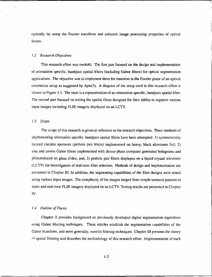
2.5 VLSI Reverse Engineering Applications .. .. .. .. ... ....... 2-6

2.6 Digital FLIR Image Segmentation .. .. .. .. ... ... ...... 2-6

2.7 Summary. .. .. ... ... ... ... ... ... ... ...... 2-9

Ill. Methodology. .. .. ... ... ... .... ... ... ... ... ....... 3-1

3.1 Introduction. .. .. .. ... ... ... ... ... .... ..... 3-1

3.2 Application of Spatial Filtering .. .. .. ... ... ... ...... 3-1

iv

Page

3.2.1 Spatial Filtering Theory .. .. .. .. ... .... ..... 3-2

3.3 Orientation Specific Bandpass Spatial Filters. .. .. .. ........ 3-4

3.3.1 Pinhole Pair Filters .. .. .. ... ... ... ........ 3-4

3.3.2 Gabor Filter CGH's. .. .. .. ... ... ... ...... 3-6

3.3.3 Real-time Filter Selection Using an LCTV. .. .. ...... 3-7

3.4 Experiment. .. .. ... ... ... ... ... ... ... ..... 3-11

3.4.1 Setup for Optical Segmentation .. .. .. ... ... ... 3-11

3.4.2 Input Images. .. .. .. .. ... ... ... .... ... 3-13

3.5 Summary .. .. .. ... ... ... .... ... ... ... ... 3-16

IV. Results and Discussions. .. .. .. ... ... ... ... ... .... ..... 4-1

4. 1 Introduction. .. .. .. ... ... ... ... ... ... ...... 4-1

4.2 Characterization of the Spatial Filters .. .. .. .. .... ....... 4-1

4.2.1 3-D3 Intensity Profiles of Filter Images .. .. .. .. ...... 4-1

4.2.2 Filter Spectrums. .. .. .. ... ... ... ... ..... 4-6

4.2.3 Comparison of Spatial Filters .. .. .. ... ... ..... 4-7

4.3 Testing Results and Discussion .. .. .. ... ... ... ...... 4-8

4.3.1 Testing With Texture Slides .. .. .. .. ... ........ 4-9

4.3.2 Testing With Template Slides .. .. .. ... ... ..... 4-10

4.3.3 Testing With Static FLIR Images. .. .. ... ... ... 4-15

4.3.4 Testing With Real-Time FLIR Imagery. .. .. .. ..... 4-19

4.4 Summary .. .. .. ... ... ... ... .... ... ... ... 4-19

V. Conclusions and Recommendations. .. .. .. ... ... ... .... ..... 5-1

5.1 Summary. .. .. ... ... ... ... ... ... ... ...... 5-1

5.2 Conclusions. .. .. .. ... ... ... ... ... ... ...... 5-2

5.3 Recommendations. .. .. .. ... ... ... ... ... ....... 5-2

V

Page

Appendix A. Detour Phase Hologram Production .. .. ... ... ... ..... A-i

A. 1 Gabor-Filter Program .. .. .. ... ... ... ... ... ..... A-i

A.2 Process and Variable Explanation .. .. .. ... ... ... ..... A-3

A.2.1 The Subroutine Gabor. .. .. .. ... ... ... ..... A-4

A.2.2 Program Operation. .. .. ... ... ... ... ..... A-5

A.3 Compiling, Previewing, Plotting, and Photoreducing. .. .. ..... A-6

A.3.1 Compiling. .. .. .. ... ... ... ... ... ..... A-6

A.3.2 Previewing. .. .. .. .. ... ... ... ... ...... A-6

A.3.3 Plotting. .. .. .. .... ... ... ... ... ..... A-6

A.3.4 Photoreducing. .. .. .. ... ... ... ... ...... A-7

Appendix B. LCTV Modifications and Limitations. .. .. .. ... ... ..... B-I

B.lI Introduction. .. .. .. ... ... ... ... ... .... ..... B-1

B.2 LCTV Theory .. .. .. .. .... ... ... ... ... ....... B-1

B.3 Modifications .. .. .. ... ... ... ... ... .... ..... B-2

B.3.1 LCTV Disassembly. .. .. .. ... ... ... ...... B-2

B.3.2 LCTV Assembly. .. .. .. .. ... ... ... ...... B-3

B.4 LCD Configuration and Spatial Resolution Limitations ...... B-3

B.4.1 LCD Configuration. .. .. ... ... ... ... ..... B-4

B.4.2 Spatial Resolution Limitations .. .. .. .. ... ....... B-5

Appendix C. Barplot Generation .. .. .. ... ... ... ... ... ...... C-i

C. I Barplot Program .. .. .. .. ... ... ... ... ... ...... C-1

C.2 Explanation of Program. .. .. .. ... ... ... ... ...... C-2

C.3 Output Procedures. .. .. .. ... ... ... ... ... ....... C-3

Appendix D. Texture Plots .. .. .. ... ... ... ... ... .... ..... D-1

Bibliography .. .. ... ... ... ... ... ... ... ... .... ... .... BIB-I

Vita .. .. .. ... ..... .... ... ... ... ... ... ... ... .... VITA-1

vi

List of Figures

Figure Page

1.1. Experimental setup for optical segmentation ........................ 1-4

2.1. Image segmentation of anisotropic white noise texture collage ......... .... 2-2

2.2. Complete 2-D Gabor transform of the anisotropic white noise mondrian dis-

played in Fig. 2.1 ......... ................................ 2-3

2.3. 2-D Fourier transforms of the Gabor elementary functions employed in one

log-polar radial octave "wavelet" scheme .......................... 2-3

2.4. a. Image of plain white cup. b. Result of summing the values measured by all

filters at each region in the image ............................... 2-4

2.5. Segmentation using two filters of different orientations .................. 2-5

2.6. Input image after preprocessing ........ ........................ 2-7

2.7. Combined Gabor transforms of rotation 20, 45, 70, 110, 135, and 160 degrees 2-8

2.8. Examples of digital FLIR segmentation using Gabor transforms ........ .... 2-10

3.1. (a) Example of a 2-D cosine Gabor function (b) 2-D Fo,'rier transform of (a) . 3-2

3.2. Common setup for spatial filtering ........ ...................... 3-3

3.3. Example of a odd impulse pair ........ ........................ 3-8

3.4. Example of a even impulse pair ........ ........................ 3-8

3.5. Example of a cosine Gabor detour-phase CGH negative ..... ........... 3-9

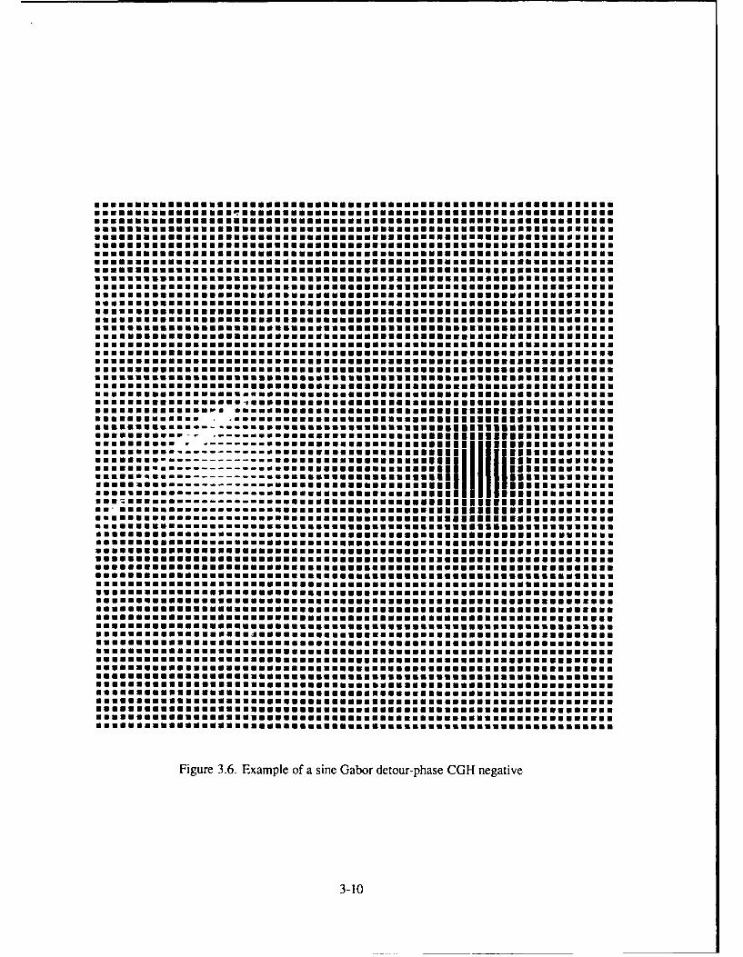
3.6. Example of a sine Gabor detour-phase CGH negative ................. 3-10

3.7. Picture of the Sony Video Walkman LCTV used in the optical bench setup . . 3-11

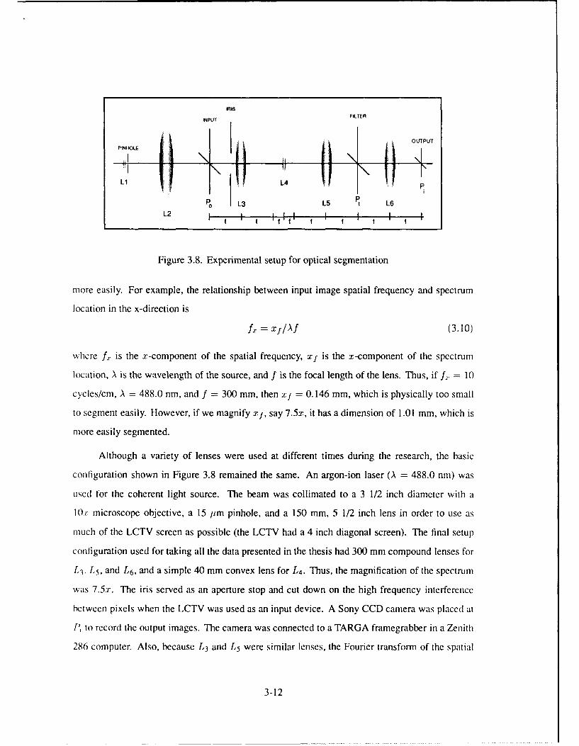
3.8. Experimental setup for optical segmentation ..... ................. 3-12

3.9. Optical setup for observing Fourier transforms of filter designs ........... 3-13

3.10. Complex texture image consisting of spatial frequencies of 10, 20, 30, 40, and

50 cycles/cm with its Fourier transform ...... .................... 3-15

3.11. Demonstration of fundamental frequency segmentation technique ....... .... 3-15

vii

Figure Page

4.1. (a) Pinhole pair filter image; (b) Its 3-D intensity profile ..... ........... 4-2

4.2. (a) Sine CGH Gabor filter image; (b) Its 3-D intensity profile ............. 4-3

4.3. (a) Cosine CGH Gabor filter image; (b) Its 3-D intensity profile ... ....... 4-4

4.4. (a) LCTV Pinhole pair filter; (b) Its 3-D intensity profile ............... 4-5

4.5. Wavelet spectral images of pinhole filters .......................... 4-6

4.6. Wavelet spectral images of three different filters ..................... 4-8

4.7. Simple texture image of two orientations at 10 cycles/cm, and its Fourier

transform .......... ................................... 4-9

4.8. Segmentation of a simple texture image using a pinhole filter ............ 4-11

4.9. Segmentation of a simple texture image using a cosine Gabor CGH filter . .. 4-11

4.10. Segmentation of a simple texture image using a sine Gabor CGH filter . . .. 4-11

4.11. Segmentation of a complex texture pattern using an pinhole pair filter . . .. 4-12

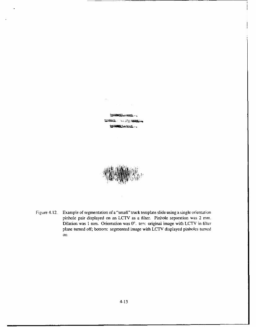
4.12. Example of segmentation of a "small" truck template slide using a single

orientation pinhole pair displayed on an LCTV as a filter. ............... 4-13

4.13. Example of a poorly segmented template slide using a pinhole filter with

apertures chosen too small ....... ........................... 4-14

4.14. Segmentation of a truck template slide using five different pinhole filters. . . 4-14

4.15. Segmentation of a multiple object template slide using a multiple orientation

pinhole filter ......... .................................. 4-15

4.16. Segmentation of static FLIR image REFJ16 using a pinhole filter ....... .... 4-16

4.17. Spectrum of Sony Walkman LCTV with circles drawn on top depicting a pinhole

filter with 4 mm separations, 2 mm dilations, and 2 orientations ... ....... 4-17

4.18. Segmentation of static FLIR image REFM13 using a pinhole filter ....... ... 4-18

4.19. Optical setup used for observing segmented and unsegmented real time FLIR

images synchronously ........ ............................. 4-20

4.20. Segmentation of two frames of real-time FLIR imagery using a circular aperture

pair filter with two orientations, 0 and 90 ....... ................. ..... 4-21

A. I. Location of gaussian regions in Gabor filter holograms ................ A-4

viii

Figure Page

B. 1. Sketch of magnified view of RGB pixel arrangement on the LCD. R-red;

G-green; B-blue ......... ................................ B-4

B.2. Sketch showing composite pixel spacing components ................. B-6

B.3. Optical setup used to observe LCTV spectrum ...... ................ B-6

B.4. Spectrum of LCTV with no input image displayed ..... .............. B-7

B.5. Spectrum of LCTV with spectral coefficients from 4 cycle/cm bar pattern

displayed showing lower resolution limit of LCTV. ................... B-8

B.6. Spectrum of LCTV with spectral coefficients from 12 cycle/cm bar pattern

displayed showing upper resolution limit of LCTV. ................... B-9

D. 1. Example of a simple texture slide with 10 cycles at two perpendicular orientations D-2

D.2. Example of a simple texture slide with a 10 cycle background and two 20 cycle

textures in parallel and perpendicular orientations .................... D-3

D.3. Example of a more complex simple texture slide with a 10 cycle background

and three other textures consisting of 30, 40, and 50 cycles at 0, 45, 90, and

1350 orientations ......... ............................... D-4

D.4. Example of a more complex simple texture slide with a 10 cycle background

and four other textures consisting of a 20 cycle center texture and 30, 40, and

50 cycle outer lobes, all at different orientations ..................... D-5

ix

List of Tables

Table Page

B.1. Mechanical Specifications of Liquid Crystal Display .......... ... B-2

x

AFIT/GEO/ENG/90D-09

Abstract

This research effort successfully implemented an automatic, optically based image segmen-

tation scheme for locating potential targets in a cluttered FLIR image. Such a design is critical to

achieve real-time segmentation and classification for machine vision applications.

The segmentation scheme used in this research was based on texture discrimination and

employs orientation specific, bandpass spatial filters as its main component. The orientation

specific, bandpass spatial filters designed during this research include symmetrically located

circular apertures implemented on heavy, black aluminum foil; cosine and sine Gabor filters

implemented with detour-phase computer generated holography photoreduced onto glass slides;

and symmetrically located circular apertures implemented on a liquid crystal television (LCTV)

for real-time filter selection.

The most successful design was the circular aperture pairs implemented on the aluminum

foil. Segmentation was illustrated for simple and complex texture slides, glass template slides,

and static and real-time FLIR imagery displayed on an LCTV.

xi

OPTICAL

IMAGE SEGMENTATION

USING

WAVELET FILTERING

TECHNIQUES

1. Introduction

This research effort extends previous research accomplished in a 1989 thesis project titled

"Gabor Transforms for Forward Looking Infrared Image Segmentation" by Kevin Ayer (3). Ayer

addressed the problem of distinguishing or "segmenting" areas of interest (potential targets) from

cluttered images using Gabor filtering techniques. In his thesis, the segmenting capabilities of

Gabor filters w.:re established with the use of computer algorithms and digitized images. Although

Ayer's segmenting techniques were highly successful in locating potential targets, the computer

algorithms used to process the images were computationally intense which severely limited the

processing speed. Furthermore, orders of magnitude of additional computations would be required

to process real-time images. For this reason, an optical implementation of his algorithm was

proposed. A review of Ayer's research and other papers that support the segmentation capabilities

of the Gabor function are presented in Chapter 11.

1.1 Problem Statement

An automatic, optically based image segmentation scheme for locating potential targets in a

cluttered FLIR image has never been implemented. The advantage of such a scheme is speed, i.e.,

the speed of light. The goal is to be able to instantaneously and automatically segment real-time

FLIR images for machine vision processing. Over the past 25 years, several segmentation

algorithms have been developed at AFIT (6, 15, 16, 31, 33, 34, 37), however, they are heuristic in

nature and use non-linear mathematical manipulation of data-algorithms not readily implemented

optically and computationally intense for real-time use (3). In contrast, image segmentation using

wavelet filtering techniques can be accomplished automatically, instantaneously, and implemented

1-1

optically by using the Fourier transform and coherent image processing properties of optical

lenses.

1.2 Research Objectives

This research effort was twofold. The first part focused on the design and implementation

of orientation specific, bandpass spatial filters (including Gabor filters) for optical segmentation

applications. The objective was to implement them for insertion in the Fourier plane of an optical

correlation setup as suggested by Ayer(3). A diagram of the setup used in this research effort is

shown in Figure 1.1. The inset is a representation of an orientation specific, bandpass spatial filter.

The second part focused on testing the spatial filters designed for their ability to segment various

input images including FLIR imagery displayed on an LCTV.

1.3 Scope

The scope of this research is given in reference to the research objectives. Three methods of

implementing orientation specific, bandpass spatial filters have been attempted: 1) symmetrically

located circular apertures (pinhole pair filters) implemented on heavy, black aluminum foil; 2)

sine and cosine Gabor filters implemented with detour-phase computer generated holograms and

photoreduced on glass slides; and, 3) pinhole pair filters displayed on a liquid crystal television

(LCTV) for investigation of real-time filter selection. Methods of design and implementation are

presented in Chapter III. In addition, the segmenting capabilities of the filter designs were tested

using various input images. The complexity of the images ranged from simple textured patterns to

static and real-time FLIR imagery displayed on an LCTV. Testing results are presented in Chapter

IV.

1.4 Outline of Thesis

Chapter II provides background on previously developed digital segmentation algorithms

using Gabor filtering techniques. These articles establish the segmentation capabilities of the

Gabor transform, and more generally, wavelet filtering techniques. Chapter III presents the theory

of spatial filtering and describes the methodology of this research effort. Implementation of each

1-2

of the three major filter designs is discussed, and details are given on the experimental setup

and implementation of the various input images. Chapter IV details the results of this research

effort. Characteristics of the three filter designs and the segmentation capabilities of the filters are

presented and discussed. Finally, conclusions and recommendations are provided in Chapter V.

1-3

0C3

a.aU

ILL

CI-Ww

-JL

-~j

0 0

Figure 1. 1. Experimental setup for optical segmentation. The inset is an orientation specific,bandpass spatial filter with circular apertures.

1-4

11. Background

2.1 Introduction

The discussion in this chapter establishes the image segmentation capabilities of the Gabor

transform. To this end, five articles are reviewed which illustrate how the Gabor transform

segments images. All five articles illustrate their segmentation techniques using computer

algorithms and static input images. None have implemented the Gabor transform optically;

however, the last article by Ayer proposes an optical implementation scheme that has been adopted

in this thesis. The first three articles describe the fundamentals of texture discrimination and

segmentation using the 2-D Gabor transform. Their segmentation examples show results using

rudimentary textured scenes as inputs. The last two articles employ the Gabor transform to solve

actual segmentation problems in the Air Force. Their segmentation examples illustrate the ability

of the Gabor function to extract desired features using complex "real world" scenes as inputs.

2.2 Original Work on 2-D Gabor Transform (11)

Daugman's work with the 2-D Gabor transform has set the foundation for using the transform

for texture discrimination. Since 1980, Daugman has steadily extended Gabor's original work

from one dimensional Gabor filters used for information compression to two dimensional Gabor

filters used for image analysis, segmentation, and compression. And, in his collaboration with

Jones and Palmer, he has promoted Gabor functions as good models for two dimensional receptive

fields of simple cells in the mammalian visual cortex.

In his 1988 article, Daugman illustrated the texture based image compression and seg-

mentation capabilities of the Gabor transform using neural networks. Texture discrimination

was achieved by examining the textural signature of an image using the Gabor transforms of

the image and grouping similar Gabor coefficients together. An illustration of this is given in

Figures 2.1 and 2.2.

In this same article, Daugman also proposed simplified versions of the Gabor function by

eliminating two degrees of freedom. He called these functions "self similar" Gabor functions.

In his "biologically motivated" implementation of these functions called the log-polar set, the

gaussian dilations and sinusoidal frequencies are distributed in octave steps and six orientations

2-1

Figure 2.1. Image segmentation of anisotropic white noise texture collage (upperleft), by thedipole clustering of coefficients in the complete 2-D Gabor transform displayed inFig. 2.2.

are used diffcring in 30' steps. This configuration, shown in Figure 2.3, appears to be a good

organization for spatial filters attempting multiple frequency and orientation segmentation.

2.3 Texture Discrimination by Gabor Transforms(38)

In 1986, Turner wrote an article supporting the Gabor transform as a good model for

"preattentive texture discrimination" in visual neuron performance. In other words, his results

suggested that Gabor transforms might be good models for spontaneous texture segmentation in

the human visual system. His work was based to a large degree on the work of Daugman, Jones,

and Palmer up through 1985.

In his article, a series of programs was created to evaluate the applicability of Gabor

functions to texture analysis. Three types ot images were used as inputs. They were characterized

by "the statistical complexity which distinguishes the different textured regions," and were

classified as first-order, second-order, and third-order differences. It was shown that, when

properly applied, Gabor functions were able to distinguish the textured regions of the images by

2-2

Figure 2.2. Complete 2-D Gabor transform of the anisotropic white noise mondrian displayedin Fig. 2.1. Different local spectral dipoles are apparent in regions of the transformcorresponding to regions of the image described by different anisotropic texturemoments.

Figure 2.3. 2-D Fourier transforms of the Gabor elementary functions employed in one log-polarradial octave "wavelet" scheme.

2-3

Figure 2.4. a. Image of plain white cup. b. Result of summing the values measured by all filtersat each region in the image.

successively reducing the statistical complexity of the images to "first-order differences in the

measured values." Turner asserts that an automatic segmentor can be developed based on the

successive reapplication of Gabor functions to textured images. He concluded that, based on his

results, Gabor functions can be used to discriminate textures in an image. The orientation specific,

bandpass spatial filters presented in this thesis can simultaneously apply multiple orientation,

frequency, and dilation filtering to the input images and, hence, act as automatic segmentors. An

example of Tumer's results using first-order statistics is given in Figure 2.4.

2.4 Texture "Demodulation" Using Gabor Transforms(5)

In their 1990 article, Bovik, Clark, and Geisler characterized image texture as a "carrier of

region information" similar to how a communications signal is modulated for transmission. In

this sense, they characterized the Gabor transform as a demodulating function which filters the

regional information from the image texture. They liken this demodulation technique to "tuning"

the orientation, radial frequency bandwidth (dilation), and center frequency of the 2-D Gabor

finction to a specific image texture.

Due to computation limitations, only a small number of filters could be employed in

2-4

(a) (b)

(C) (d)

(e)

Figure 2.5. Segmentation using two filters of different orientations: a. original; b. Fouriertransform; c.,d. channel amplitudes recovered; e. computed texture boundaries.

their algorithm at one time. Thus, guidelines were given for filter selection based on a simple

peak-finding algorithm applied to the image power spectrum. Using these guidelines, a "computer

vision" model was developed and applied to both synthetically generated and naturally occurring

textures. An example of their segmentation results is given in Figure 2.5.

Although this technique did not select an optimal Gabor filter set, their results demonstrated

the ability of the Gabor transform to achieve segmentation using only a subset of the information

within each texture. They concluded that the Gabor transform is a "feasible approach to segmenting

image texture in a predictable manner" and proposed that new algorithms should be developed

for using the Gabor transform for edge and motion detection. However, they deemed the "most

difficult problem" to be the "development of fast algorithms and architectures for filtering an

image to a large set of Gabor filters" due to computation limitations. Indeed, speed limitations

are major obstacles for computer based algorithms, but they pose no problem for optically based

2-5

algorithms like the one developed in this thesis.

2.5 VLSI Reverse Engineering Applications (28)

In his 1989 thesis, Mueller employed Gabor transforms to segment out the contacts in

VLSI circuits to assist in reverse engineering the circuits. The VLSI circuit diagrams were

digitized using a camera and a video image processing board. Mueller used computer algorithms

for processing all the image information including the Gabor transforms. Before segmentation

processing, the images were preprocessed by normalizing the brightness of the individual image

pixels and enhancing their contrasts.

Various combinations of orientations, pitch, and frequency of Gabor functions were

investigated, and guidelines were developed for their use. An interesting result was Mueller's

choice of orientations for his Gabor filters. Because the contacts were circular, all orientations of

the Gabor filter should be equally likely to segment the contacts from the background features.

However, because most of the other features in the VLSI circuit (which he did not desire to

segment) were oriented at angles of 0 and 90, these two common orientations were not used.

Consequently, he chose the orientations at angles of of 20, 45, 70, 110, 135, and 160 in order to

equalize the spacing between rotations and achieved excellent results. He concluded that "Gabor

processing is a viable technique for contact segmentation." An example of his results is shown in

Figures 2.6 and 2.7.

2.6 Digital FLIR Image Segmentation (3)

In his 1989 thesis, Ayer employed Gabor transforms to segment out targets in cluttered

Forward Looking InfraRed (FLIR) images. He used computer algorithms for processing all the

image information including the Gabor transform. The FLIR images were preprocessed before

segmentation by normalizing the brightness of the image pixel values and post-processed by

thresholding and binarizing the pixel values.

Both sine and cosine Gabor functions were investigated for their segmentation abilities in

Ayer's research. To this end, he demonstrated that sine Gabor functions act as "edge detectors"

and cosine Gabor functions act as "body fillers." He used orientations of 0, 45, 90, and 135

2-6

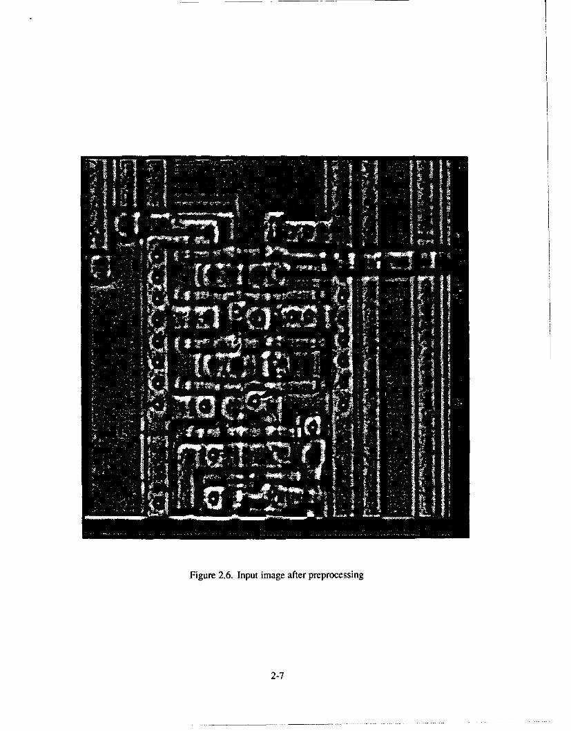
Figure 2.6. Input image after preprocessing

2-7

Figure 2.7. Combined Gabor transforms of rotation 20, 45, 70, 110, 135, and 160 degrees

2-8

degrees, because these were the orientations most prevalent in the targets. He concluded that "in

combination, sine and cosine Gabor functions produce fully segmented targets" from the cluttered

FLIR images. Binarized images segmented using his techniques are shown in Figure 2.8.

Ayer also proposed an optical implementation scheme for segmenting images using Gabor

transforms which was adopted in this research. His scheme was based on implementing Gabor

filters as computer generated holograms and using spatial filtering techniques to segment the

images.

2.7 Summary

The five articles reviewed established the digital segmentation capability of the Gabor

transform using computer algorithms and static images. They all base their findings on the ability

of the transform to discriminate between texture frequency, orientation, and localization. Daugman

and Turner's use of the Gabor transform was biologically motivated. They see the transform as a

possible answer to modeling the perceptive field of a cortical neuron. Bovik, et al., applied the

Gabor transform as a spatial filter and provided insight into efficient filter selection. Mueller and

Ayer provided successful illustrations of segmentation using the Gabor transform applied to real

world problems. However, all were limited in speed due to relatively slow digital computations of

2-D Fast Fourier Transforms (FFTs) and were unable to segment real-time imagery. The optical

algorithm developed in this thesis is capable of instantaneouIs 2-D FFTs which makes it perfectly

suited for segmenting real-time imagery.

2-9

... .. ... ... .. ... .

llc

i,~,

Figure 2.8. Examples of digital FLIR segmentation using Gabor transforms. Original FLIRimage (top); Binary version of sine Gabor transform of top image: edge detection(middle); and Binary version of cosine Gabor transform of top image: body filling(bottom)

2-10

1II. Methodo!ogy

3.1 Introduction

The discussion in this chapter outlines the theory of optical spatial filtering and methods of

implementation and testing of optical spatial filters as applied to texture discrimination and image

segmentation. Chapter organization is divided into three parts. The first part focuses on the theory

of optical spatial filtering and its application to texture discrimination. The second part focuses on

the design and implementation of texture discriminate optical spatial filters. Implementations of

these filters included simple pinholes punched in heavy, black aluminum foil, computer generated

holograms (CGH's) of sine and cosine Gabor filters, and pinhole pairs displayed on a liquid crystal

television (LCTV). The third part focuses on the design and implementation of the optical bench

setup and a variety of input images used to test the optical spatial filters. Complexity of the input

images ranged from simple textures on glass slides to real-time FLIR imagery displayed on an

LCTV. The results from these tests are described and discussed in Chapter IV.

3.2 Application of Spatial Filtering

Spatial filtering is used to optically implement the segmentation algorithms presented in the

Ayer thesis (3). Ayer's underlying methodology was to segment the objects in an input image by

correlating Gabor filters with the input image. He digitally implemented the Gabor filters and

the input image in the space domain, computed their fast Fourier transforms (FFT's), multiplied

the two FFT's together, and then computed the inverse FFT of the product. To achi ye multiple

orientation, frequency, and dilation filtering, correlation intensities resulting from computa-tions

with a filter at a single orientation, frequency, and dilation were added together - analogous to

incoherent imaging (linear in intensity).

Although the underlying methodology of this thesis remains the same as the Ayer thesis,

the optical filters used were implemented in the frequency domain rather than the space domain.

Because the algorithm was implemented using coherent imaging, individual correlations must be

added together on a complex amplitude basis. Thus, multiple orientation, frequency, and dilation

filtering was realized with a single spatial filter implemented in the frequency domain (linear in

3-1

Gabor Function Frequency Response

(a) (b)

Figure 3.1. (a) Example of a 2-D cosine Gabor function (b) 2-D Fourier transform of (a)

complex amplitude). An example of a 2-D cosine Gabor function (space domain) and its 2-D

Fourier transform (frequency domain) is given in Figure 3.1 (11).

3.2.1 Spatial Filtering Theory In this thesis, two-dimensional Fourier transforms are used

to resolve an input image into its spectrum: a set of paired Fourier coefficients that represent

a system of sine and cosine functions which contain all the information of the original image.

Each coefficient pair represents a specific spatial frequency and orientation at some amplitude and

phase.

In optical image processing, spatial filtering implies physically obstructing or modifying a

portion of the spectrum of the input image. The most common setup for optical spatial filtering in

a coherent imaging system is shown in Figure 3.2.

In this setup, called a 4-f setup, collimated light from a laser acts as a plane wave

source incident on an input image (object) located at P,. The transform lens, Lt, pcrforms a

two-dimensional Fourier transform of the object which is focused at Pi. The "inverse" transform

lens, Li, performs a two-dimensional "inverse" Fourier transform of the spectrum at Pt which is

focused at Pi. If no spatial filter is placed at Pt, the output image at Pi is the same as the input

image with some scaling depending on the focal lengths of the lenses and with some blurring

depending on the diameters of the lenses. However, if a portion of the spectrum is obstructed by a

3-2

INPUT FILTER OUTPUT

PO L t Pt Li P i

I f I I f I f I

Figure 3.2. Common setup for spatial filtering

spatial filter, the output image can be altered in significant ways (13:87, 141, 167).

Mathematically, spatial filtering in a coherent imaging system can be represented as a

two-dimensional convolution between the input image and the inverse Fourier transform of the

spatial filter. Goodman (13:166) derived this convolution relationship for the intensity distribution

of a 4-f system:

I(x2 , y2) = KI JJ g( , ,I)h(xi - ,y - q1) d dy,!2 (3.1)I~~Y, y0)

where, K is a constant, g represents a space-varying amplitude transmittance function of the

input image at P, and h represents the inverse Fourier transform of the space-varying amplitude

transmittance function of the spatial filter at P. Note that if h is given by

h(x, y) = si(-x, -y) (3.2)

thcn the relationship can be thought of as the crosscorrelation of g aiid s (1 3:178).

3-3

3.3 Orientation Specific Bandpass Spatial Filters

The segmentation filters designed in this thesis can be classified as orientation specific band-

pass spatial filters. Orientation specific bandpass spatial filtering implies frequency discrimination

or "textural" discrimination at a specific orientation of the texture. According to Bovik,et.al. (5),

textures can be modeled as "irradiance patterns distinguished by a high concentration of localized

spatial frequencies." Where "distinct textures are characterized as differing significantly in their

dominant spatial frequencies." Thus, optically segmenting distinct textures should only require

passing their dominant spatial frequencies through symmetric apertures at appropriate separations

and orientations and blocking out the rest of the spectrum. Now the question is raised: how can

one determine the dominant spatial frequencies of a group of textures or an input image?

Bovik provided a simple way to choose dominant frequencies when an image contained

two discriminable texture regions based on the following criteria: "For strongly oriented textures,

the most significant spectral peak along the orientation was chosen [as the dominant frequency].

For periodic textures, the lower fundamental frequency was chosen [as the dominant frequency].

Finally, for non-oriented textures, the center [dominanti frequencies were chosen from the two

largest maxima (5)." This research effort identified dominant spatial frequencies in a similar

manner to Bovik's method by simply looking at the spectrum for the brightest spectral peak(s)

(other than DC) along a specific orientation.

Of course, the apertures chosen to pass the spatial frequency components were gaussian

pairs, i.e., Fourier transforms of Gabor functions. However, due to ease of implementation,

pinhole pairs were initially used to demonstrate coarse texture segmentation. The implementation

of both the pinhole pairs and the gaussian pairs are described in the following paragraphs.

3.3.1 Pinhole Pair Filters Pinhole pair filters are nothing more than symmetrically

located circular apertures. In the space domain, one could think of them as Airy disc wavelets.

In other words, if we model the circular apertures as having constant intensity across them, then

the transmittance function of a symmetric aperture pair can be expressed mathematically in the

frequency domain as:

T(. 71) = circ 4,71 - o, - 71o) + 5( + o, y + yo)] (3.3)

3-4

where:

circ (-1 / (3.4)

S{ 10 otherwise

"" represents a convolution, 6 represents a delta function, p = v/' + r/2, o represents a distance

along the direction, qjo represents a distance along the 7) direction, and I represents the pinhole

dilation (diameter).

Thus, the "inverse" Fourier transform of the symmetric aperture pair can be expressed

mathematically in the space domain as an Airy disc wavelet:

(/)2 J1 (rlr) _

t(x, y) = (lr) cos (27r( ox + ?joy)) (3.5)

where, r = v/x 2 +Y 2 and J1 represents a first-order Bessel function.

Furthermore, Goodman (13:66) derived the intensity of an Airy disc which, combined with

the square of the sinusoid, gives the intensity function of the Airy disc wavelet:

I(x, Y) = ft(x, y)12 = 2 J1 (rlr/Af) 2 0.5 [1 + cos(2r[2 o(x + y)])] (3.6)[(7rlr/A-f)jwhere it was assumed that o = 77o.

Using Equation 3.6, the number of cycles in the middle lobe of the Airy disc can be

predicted. If ro is the distance from the origin to the first zero crossing of the Airy disc, then

1.224ro = - (3.7)

Additionally, the spatial frequency of the wavelet can be given in terms of

= 2(3.8)Af

Thus, the number of cycles over the total lobe can be calculated from Equations 3.7 and 3.8 as:

#cycles = 4.88p (39)centerlobe 2ro2 0 -

3-5

For example, if the aperture separation is 2 mm (p 1 mm) and the aperture dilation, 1, is 1 mm,

then the number of cycles per middle Airy disc lobe should be 4.88 cycles/lobe. Note that this

result is independent of the wavelength of the laser light or the focal length of the lens.

The implementation of the pinhole pair filters was trivial and only required that some medium

be placed in the filter plane that could be impressed with small circular apertures (pinholes) to

pass the desired spectral coefficients and block the rest of the image spectrum. The medium of

choice was heavy, black aluminum foil, since it was readily available, required no special tools or

software to manipulate (i.e., drill press or computer), and retained its shape fairly well (some slight

microscopic tearing was unavoidable). The filters were made by cutting and smoothing 5 cm x

5 cm pieces of foil, then impressing circular aperture pairs into them using a pin. The apertures

were placed along a common axis symmetrical to an origin (middle of the foil). Separations of

apertures varied from 2 mm to 12 mm. Diameters of apertures varied from about .5 mm to 3 mm.

Orientations were not limited since the filters were placed in a rotating mount with a 3600 range.

Characteristics of the pinhole pair filters are given in Chapter IV.

33.2 Gabor Filter CGH's Like the pinhole pair filters, Gabor filters are gaussian aperture

pairs placed along a common axis symmetric to some origin. However, creating the gaussian

apertures was not trivial. Three general methods of implementing the gaussian apertures were

determined feasible. These methods were 1) encode the gaussians mathematically into detour-

phase computer generated holographs (CGH's), output the holographs onto transparencies, and

photoreduce onto glass slides. 2) Coherently image a gaussian apodizer (obtained from Lt

Col James Mills (26)) onto either glass slides or thermal plastic using two lens imaging and a

translatable mount. 3) Create grey-scale gaussian filters on the computer, output to transparencies,

and photoreduce onto glass slides.

Due to time restraints, only the detour-phase CGH method of implementing the Gabor

filters was pursued. The advantage of detour-phase CGH's over the other two methods was the

availability of a detour-phase CGH program that had already been written by a previous AFIT

student, Vicky Robinson (32). Although modification of the program was necessary, at least

some precedent had been set for implementation of the holograms. A good explanation of the

theory behind detour-phase holography applied toward amplitude holograms can be found in the

3-6

Robinson thesis or in Reference (21).

The CGH program written to generate Gabor filters in the frequency domain makes a

distinction between sine and cosine Gabor functions. Recall that a simple sine function in the

space domain can be represented in the frequency domain by an odd impulse pair, Figure 3.3, and

a simple cosine function in the space domain can be represented in the frequency domain by an

even impulse pair, Figure 3.4 (12). Thus, a single frequency, single orientation cosine Gabor filter

can be realized by two symmetrically located gaussian apertures of equal transmittance with their

background set as close to zero as possible (recall Figure 3.1b). However, in order to realize a

similar sine Gabor filter, its background must be shifted up from zero by half the amplitude of the

positive part so that the peak of the negative part has zero transmittance, and the net effect is an

odd gaussian pair with an incorporated DC bias.

A detailed description of the CGH program used, output procedures, and photoreduction

procedures followed in making the CGH's are given in Appendix A. The program produces

the "negative" of the desired output, because the photoreduction process reverses the image.

Examples of sine and cosine Gabor detour-phase CGH negatives are given in Figures 3.5 and 3.6.

Characteristics of the Gabor filters and comparisons to pinhole pair filters are given in Chapter Fl.

3.3.3 Real-time Filter Selection Using an LCTV A Sony Video Walkman liquid crystal

television (LCTV) with a built-in 8 mm VCR was used as an amplitude spatial light modulator

(SLM) for investigating real-time display of spatial filters and input images in the optical bench

setup. The LCTV used is pictured in Figure 3.7. This section describes how the pinhole filters

were displayed on the LCTV. Section 3.4.2 describes how the input images were displayed on the

LCTV.

Pinhole pairs were displayed on the LCTV by the use of a Panasonic Video Camera on a

tripod mount. The video output of the camera was connected to the video input of the LCTV

with the LCTV switched to "line" mode. Pinholes were impressed into black aluminum foil and

backlit by a directional white light source. The camera was then focused onto various separations

of pinholes until the desired combination was found. A 2.5:1 ratio of pinhole separation distance

on foil to pinhole separation distance on the LCTV was observed. For example, a 5 mm separation

on the aluminum foil corresponded to a 2 mm separation on the LCTV.

3-7

H(j)= Ft sin(24tox) I

Figure 3.3. Example of a odd impulse pair

H(j)= F Icos(2rr~0 x))

Figure 3.4. Example of a even impulse pair

3-8

-- - - ----- -- -- -- --- -- -- -- -- - - u..u .--- --------------------- -mu.**mm..---------------------------- UlhU m---------------------------------- l-u------------------------------umml3.------------- -- -- --- -- ---- ----- --------------------------iU EE ll3f U ------- -- -- -- -- -- -- -- -- -- -- -- --------------------------mu lh l h u--- --- -- --- --- ----------------------------- -IE E1--------------- -- --- - m- -- - - ------------------------ - - - - - --- --- - - -- - -- - - -- - - -- - -- - - -- ---------"::Ii : :: --------- ---- - - -- - - - -- - - -- - - - -- - - -- - -----------ul l l E u--- -- -- -- -- -- -- -- ------------------- m ~ lu-------------------

- -- - - - - - - - - - - - - - - - - - - - - - - - - - - - - - - - ----mu l m m-- -- -U U-- - - - - - - --u- - - - - - - - - - --u m- --m- -u- -- -- - - - - l m - - - - - - - - - - - - - - - - - - - - - - - - - - - -

-- Figure-3..-Example-f-a-cosine-abor-deto-phase CGH negative----

--------- --------- ------- - 9- - - - - - - - -- - - - - - - -

* uUmUmmuUEuEEUUmEuEUmUEuUEEUUEUmUUUUmmUmmmmEuUEEUuEmUmUUUu mm....U.... mummmuUEUmEE~*EUUUEUUmummUmUUumUmmummmUUUUUEuUmmEmmEUEEEEEmmU.... mmmmmmmmuumummumummumummummmmmuummmmmummuummmm.mmmm.mmmmmmm.uuuuumuuuuuu...uuu.u.m..mmu....muum...uuu..mmmmmmu..u.u.. mum...umuEm mu umummuummmmmmmuuumumummmmmmummuummumummumUmumuuuuuuamuummmm..... .. m..uu.....m.muu......m.um.mmm.mmu.u.umum..mUmm.m....u..mm..... muUmuummmmuUUm.ummm.mmmu..mmuu...mmmUEmmUmUm.mmumumumummuU...... EUmmuUumUUummmmmmmUmmUUUmUuUmUEEEEUUmummmmuUuUmuEuUUmUmu.mummuEm .u.uuu.u..um.mm..m..mumm...m..u..muumm.u........mmmmu mm..mu... uumuu..Uuuuuuuuuuuuu.uuuu.u.mmmmuu.UUu.u.mmgm.uEum EUEU mumummu.mu.uummuumuuumu.uuum.um.mmmumuummuuuuumummmumummummmmu.mu mum.mu... mmuUmuummuUmumuUmumm.EUmumuEUmmmumUuEumuEmuummmmEmmmmUUEEmmuUmUmmUUUmUEUUmUmUUummUmmUUmUmUUUUUmUUuuuEUUUEUEumumUEEUmEmU mm..Eu.. ... u..um....muuu.mu.umum...u...muuu.ummmm....m.u.mmu..mu mum.U.K. mEEUUEumEEuUUUUumUUmUmUmmUmEEmUmUUEUEEEEUEEUEUUUEUuuUEUE mu..UUUUUUSUUUUUUUUUUUUUUUUUUuuUUUuUUUUUUUUEUUUDUUUUUU3UEUUU*EUEUU mmmum mumummuumm.umuumuumm...umm.mmm.mmumEUmmmm.UmumuuuUmummu.mumuu* muumu...uu.mm...m.uu.mu.uum.mumu.m.uuuummmm..mmm.uuuumu.muuu.uumm. uUEUEEUUUUUmEmuEmUuUumUuUmmmEUEUUUmmuEUEEuUEEUUUmUumUUmUmmuUm* mmUmummummmummuUummmUuumummmmUumumUmmuummumUUmEmuaUUUUmuUUmmmUu* U UmUUmUUUUUumEmEmummUUUUUuUUmUUUUEUUumUUUuUUUUUEUUmUUEUmuUUmmmm* U mmmuuuuuuuuuuuuuuuuuuuuuuuuumumuuuumumuuuuuummmuumumumm mm.....umuUmummuummmmUmmmuEmuEUmmmum.UumummmmugmmU...Uu..u.ummmmummuUUm* .u....mmummm.u..u m.uemu..ummmummummmmmmummmmmuummmmmmmmmmmmumuum...um...u..mm...u *immmummmuumUmummmEEumumEUEEEEUUEUEUmUUumUUuUUU*..UUUumUUmu..wu uu.mu.uuumumummmmmmm.muummmmmmuU*um.mumummmummm.mm.m.mm....w ~uuumummmmummuuummuuumummmmEEUEEUUEmUumummmuumm.

----------uuuuuuuuumumgmuuuuuuuuuuuUulllluuluuuuumuuumm.mmu.u.mu.w~-.- .~~~~uuummmmmummmmummummmmmmmhIuIhUUEuuEEuuummmumm.mmmmuu.u. ~----~~.u.mmu.um.m..umu....mm.uuu U.. UUEUmummuummumuumummum..------------------.ummumuumumumumEmmmmaEhI .111mm UEUUmEmumuumu

--------------.mmmumummmumuuum.mmmuuuI I 11111 UUmEmumuummuu.. u..u.uu-----------------.mummmumumugummmmmmumuUll I II... EUuumummmummm-------------.. umumuuuummuuuuuuumuul EllEN UUUUuUuUUUuuum*u*u**uu------------------muuuuEmmumuEmuuuuuuuEEII mliii~ EhUEmu.uum.mmumumummum.-------------m.mmmuuummum.muuuuummuEII *UUmmmmEmumEmmuu.~muuu.m---------------umumuuummmuum.mummmummmEuUEUEuuEEmEmm.mmmu.mmm- ummUmEminum~~inmumUUmumummmmmummmumuummmUuUUUUUmmmmmmmmummuu*umuUmuUmuUmuuwu mmmm.mmmmummummmm.mmmmmrnUu UUIUEEUUUEUmuEummmumummm...uum mum.... .... m..m.u m.Umu....m....m..3..USUU..3U..uu3UuUu..****u mm..ummmmmuum....*** mmmmmummmmummummmumuUlurnUrnummmmumummmmm.. uuu...u....muu.umu.mm.u E.mUUEEEEUUUUUEEUUEUEUEEUUUUUUUUuUEuu Emumm.mmmmmm*u...*mmmmmu.mm .mmmm..ummm.mm.m.um.m.u...um.....mmmu mmumu*mum.m.m..um.mumu..muu mUmUUuUmUEUmUUUuEumUUUUUUUUUEmuEmmUUmumu.m*um*u.*ummmu*mmmm..mmm mmummmu.U......uummmm**um*.mm mummumum..mm...... mmmmm.u ... m...m. U UUUUUUUUUUUEUUUUEUUUCUUUUUUUUUUEUUuu mu.mum .mmmm mummum U mmmmmummmm u U mmumm.mm..uum..ummmm.uummmm m u mum mu u m auummmuumuummu..um.umumu.um.mm.mmmmmuummummmmmmumummmmmmumuuumumu*mm..ummuumumummmummmmmuu .. mg.ummmmuUmmmummmmumummuummurnmmuuuu..umummummmmuUmmUflmumumummm.........m....u...um...u.mum...mmmuuuummmmumummmuuuuuummmmummmmu mmummmmmummmummuummmummmmmummum mmumm mummm.... ummmuu U muumuuuummm.umuu.mu.uu.u..uu..uum.u.umumum ummum. mm.uUUUUmUuUUuUUuUUUmUJUmmuUU...u...U.m....m.U.U.Uu.mm.U...........mum.m.u..mummum.m.u.umu.ummmum.m.um..m..um....mu....mumu.u.mm.uumummmmmmmmuummmumuuumumum..m...mm...mm..mmu.m.m.mmumm...mmmuumm.mumumummuumummmmmuuumumummmummummumm.umuummumumummmumumuuummummmmuumuummmummmmmmmmuummmmm mmmmmmmmmmmmmmmummmummumumumuuuuu mm....ummmuu mmmu mum mmmmm.mmm... ... uum.mm..m. muuummuuummuumuuuumuuuu.uumu mm muum mu m m m..mum.m.uu U mummmummmumuu m ummm mmmummmmummuum mu mum mu mmuuummmmmuummmmmmmmummmummmmmm.muummummmmmmmmm.mmmuumummu.mmmmummm mu uummuum m mmmmmuu mu mm mu mu mumummummum umm mmmmmmmum..mmmmmm m umumumumummummummummum. mmmuummmummmummummmu mumumummmmummummmmmuumm.uum muum mmmummum mm.... ummmu mumuummummm.m m mmmmmm mummm mumma mu mum.....mm. mum umum. mm mumm mm mum. mmum.mmmumum..mmmuuumuummm.mumu.uummuummu

Figure 3.6. Example of a sine Gabor detour-phase CGH negative

3-10

Figure 3.7. Picture of the Sony Video Walkman LCTV used in the optical bench setup

Specifications of the LCTV and details of the modifications necessary for use in the optical

bench setup are given in Appendix B. Characteristics of the pinhole filters displayed on the LCTV

are given in Chapter IV.

3.4 Experiment

This section describes the experimental setup used for optical segmentation and explains

the design and implementation of the input images used for testing the three spatial filter designs.

3.4.1 Setup for Optical Segmentation The basic setup used to perform optical segmenta-

tion in this thesis is given in Figure 3.8. Input images were placed at Po, and spatial filters were

placed at P. The only difference between this setup and the general spatial filtering setup shown

in Figure 3.2 is two extra lenses which increase the size of the input image spectrum incident on

the spatial filter at P1. Hence, this setup could be called an 8-f setup. An increase in the spectrum

size allows the individual spatial frequencies (diffraction orders) to be identified and segmented

3-11

IRIS

INPUT FILTER

OUTPUTPINHOLE

L3 L5 L6

L2 i i I I I I I I

Figure 3.8. Experimental setup for optical segmentation

more easily. For example, the relationship between input image spatial frequency and spectrum

location in the x-direction is

x = xf/Af (3.10)

where f. is the x-component of the spatial frequency, rf is the x-component of the spectrum

location, X is the wavelength of the source, and f is the focal length of the lens. Thus, if f, = 10

cycles/cm, A = 488.0 nm, and f = 300 mm, then xf = 0.146 mm, which is physically too small

to segment easily. However, if we magnify if, say 7.5x, it has a dimension of 1.01 mm, which is

more easily segmented.

Although a variety of lenses were used at different times during the research, the basic

configuration shown in Figure 3.8 remained the same. An argon-ion laser (A = 488.0 nm) was

used for the coherent light source. The beam was collimated to a 3 1/2 inch diameter with a

lOx microscope objective, a 15 /pm pinhole, and a 150 mm, 5 1/2 inch lens in order to use as

much of the LCTV screen as possible (the LCTV had a 4 inch diagonal screen). The final setup

configuration used for taking all the data presented in the thesis had 300 mm compound lenses for

[3. L5 , and L 6 , and a simple 40 mm convex lens for L 4 . Thus, the magnification of the spectrum

was 7.5x. The iris served as an aperture stop and cut down on the high frequency interference

hetween pixels when the LCTV was used as an input device. A Sony CCD camera was placed at

P, to record the output images. The camera was connected to a TARGA framegrabber in a Zenith

286 computer. Also, because L 3 and L 5 were similar lenses, the Fourier transform of the spatial

3-12

FILTER

L3

OUTPUT

CCD CAMERA

Pt

P0

FRAMEGRABBER

Figure 3.9. Optical setup for observing Fourier transforms of filter designs

filters could be recorded without changing the basic configuration. This was done by placing

a filter at P and observing the Fourier transform of the filter with the CCD camera at Pt (see

Figure 3.9).

3.4.2 Input Images Input images varied from simple line textures to static and real-time

FLIR images displayed on an LCTV. The primary purpose of the input images was for testing the

spatial filters and determining the optimum filter designs and configurations.

3.4.2.1 Texture Slides The input texture slides were made to test the spatial filters for

simple texture segmentation. The texture slides contained combinations of bar pattern frequencies

of 10, 20, 30, 40, and 50 cycles/cm. These frequencies were considered to be the "fundamental"

spatial frequencies of the texture slides.

The methodology for segmenting a bar pattern was based on passing the fundamental or

first-order spectral coefficients (symmetrically paired) corresponding to the fundamental frequency

of the bar pattern. Using Equation 3.10 and taking into account the 7.5x spectrum magnification,

3-13

the separations of the first-order nectral coefficients, 2xf, were calculated to be approximately

2.2, 4.4, 6.6, 8.8, and 11 mm, respectively.

For example, the irregular texture pattern shown with its Fourier transform in Figure 3.10

consists of spatial frequencies of 20, 30, 40, and 50 cycles/cm set against a background of 10

cycles/cm. Using the fundamental frequency methodology for segmenting the irregular pattern

from the background would entail passing the first-order spectral coefficients circled in Figure 3.11

and blocking the rest of the sp( trum. The results of segmenting the texture slides are presented

in Chapter IV.

The texture slides were made by modifying the CGH FORTRAN code given in Appendix

A to generate bar plots of various frequencies. Next, some "cut and paste" was performed on the

out,-'; plots, and the results were transferred to transparencies with a photocopier. Finally, the

transparencies were photoreduced by 20j- to a 1 cm x 1 cm size on glass slides. The FORTRAN

code used to generate the bar plots is given in Appendix C; texture plots are shown in Appendix D.

3.4.2.2 Template Slides The next level of segmentation testing involved segmenting

simple shapes and objects (silhouettes) of constant irradiance and no background clutter. Although

the template slides are essentially "pre-segmented", they were the next logical step to segmenting

FLIR images by helping to calibrate and optimize the aperture spacings and dilations. This was

accomplished using template slides of large and small squares, circles, triangles, letters, tanks,

trucks, and F-I5's. These slides were already available in the lab from previous experiments, and

no modifications were necessary. The results of segmenting the texture slides are presented in

Chapter IV.

3.4.2.3 Static FLIR Images on an LCTV The static FLIR input images were used

to test the spatial filters for their ability to segment objects in cluttered background. The FLIR

images segmented were the REFJ series and REFM series, which were the same ones used by

Aver (3). An LCTV SLM was used as the input medium for the static FLIR images in order to

lay the ground work for inputting real-time FLIR images. Although the resolution of the LCTV is

poor compared to other SLMs, the requirement for grey-scale capability in real-time necessitated

the use of the LCTV.

3-14

Figure 3.10. Complex texture image consisting of spatial frequencies of 10, 20, 30, 40, and 50cycles/cm with its Fourier transform

Figure 3.11. Demonstration of fundamental frequency segmentation technique. Circled spectralcoefficients corresponding to the fundamental frequencies would be passed and allelse blocked.

3-15

The images were displayed on the LCTV by connecting the TARGA framegrabber video

output cable to the video input plug of the LCTV and switching the LCTV to "line" mode. The

FUR images had previously been translated to TARGA format by John Cline (10:120). No

enhancements or preprocessing of any kind were performed on the input FLIR images. The

TARGA FLIR files all had a .HLF suffix and had been reduced from an original 240 x 640 pixels

to 71 x 320 pixels. Placing them at a specific location on the LCTV required using the user

interactive vendor program TESITARG.EXE which was supplied with the TARGA 8 board when

it was purchased. TESTTARG.EXE allows direct access to individual TARGA commands like

GETPIC, PUTPIC, LIVE, DIS, ERASE, GRAB, etc. To center the FLIR image on the LCTV,

the TARGA command GETPIC was used, and the bottom left-hand comer of the FLIR image

was placed at pixel location (100, 200), i.e. (x,, ye), on a 512 x 512 screen. Another vendor

program, TRUEART.EXE, was also available, and it was mouse-driven. However, it was a

canned program and did not allow direct access to the TARGA commands for specific placement

of images. Documentation for both programs and descriptions of TARGA commands are included

in the TARGA 8 manuals (1, 2). Also, an excellent overview of the TARGA 8 system and a

plethora of batch files written for the TARGA 8 system can be found in the Cline thesis (10).

3.4.2.4 Real-time FIR Imagery on an LCTV Real-time FLIR input imagery was

used to test the spatial filters for their ability to segment objects in cluttered background in real

time. The imagery was made available through Osvaldo Perez (30) and dubbed onto an LCTV 8

mm VCR tape. It was then played back with the LCTV in the optical setup. No enhancements or

preprocessing of any kind were performed on the input FLIR imagery.

3.5 Summary

This chapter presented the theory and methodology behind implementing orientation

specific, bandpass spatial filters designed to discriminate texture based on passing dominant spatial

frequencies at specific orientations using symmetric aperture pairs. Three major filter designs were

described: 1) symmetrically located circular apertures (pinhole pair filters) implemented on heavy,

black aluminum foil; 2) sine and cosine Gabor filters implemiited with detour-phase computer

generated holograms and photoreduced on glass slides; and, 3) pinhole pair filters displayed on an

3-16

LCTV for real-time filter selection. Also, the method of testing the spatial filters designed was

presented by describing the experimental setup and the design and implementation of the input

images.

3-17

IV. Results and Discussions

4.1 Introduction

This chapter presents and discusses the results from characterizing and testing the three

different implementations of orientation specific, bandpass spatial filters. Characterization was

performed as one way of comparing the filter implementations based on their intensity profiles and

their associated wavelet patterns. Testing the spatial filters determined how well the different filter

implementations could segment the various input images and how well the optical segmentation

results compared with the digital segmentation results from the Ayer thesis (3) No preprocessing

or post-processing of the input images was done in any way in acquiring these results. Also note

that many of the digitized camera images presented were reversed imaged, i.e., light areas are

presented dark and dark areas are presented light. This was done to highlight the areas of interest

better (and save on toner).

4.2 Characterization of the Spatial Filters

Characterization of the spatial filters was based on three dimensional intensity profiles of the

filter images and two dimensional intensity images of the filter spectrums (the wavelet patterns).

The 3-D intensity profiles were created on the SPIRICON system using filter images that weie

originally captured by the Sony CCD camera and TARGA framegrabber combination and then

were translated to SPIRICON format using the conversion program TAR2SPIR.EXE written by

Cline (10).

4.2.1 3-D Intensity Profiles of Filter Images Figures 4.1, 4.2, 4.3, and 4.4 show the three

dimensional intensity profiles of the four different types of orientation specific, bandpass spatial

filters that were implemented in this thesis: pinhole pairs on foil, sine and cosine Gabor detour-

phase CGHs, and pinhole pairs on an LCTV. Each of the four filters had a pair of symmetrically

located apertures with separations and dilations of approximately 2 mm and 1 mm, respectively.

Figure 4.1 shows an image of the pinhole filter on foil and its 3-D intensity profile. Note

the sharp cutoff at the edge of the circular aperture which causes the higher order harmonics of

the Airy disc pattern in its spectrum shown in Figure 4.6a. Figure 4.2 shows an image of the

4-1

(a)

(b)

Figure 4. 1. (a) Pinhole pair filter image; (b) Its 3-D intensity profile

4-2

Figure 4.2. (a) Sine CGH Gabor filter image; (b) Its 3-D intensity profile

4-3

(a)

(b)

Figure 4.3. (a) Cosine CGH Gabor filter imagv" (b) Its 3-D intensity profile

4-4

(a)

(b)

Figure 4.4. (a) LCTV Pinhole pair filter; (b) Its 3-D intensity profile

4-5

. b.

C. d.

Figure 4.5. Wavelet spectral images of pinhole filters: a. s=2 mm d=.5 mm, o--O; b. 2,.5,90';c. 2,1,00; d. 4,.5,0'

sine Gabor CGH and its 3-D intensity profile. Its 3-D profile appears to be a odd gaussian pair,

however, its 2-D Fourier transform did not produce a wavelet. This was probably due to the lack

of contrast between the peaks of the image. Thus, no wavelet image is given for the sine CGH in

Figure 4.6. Figure 4.3 shows an image of the cosine Gabor CGH and its 3-D intensity profile. Note

the smooth gaussian shape of the apertures and the corresponding gaussian shape of its spectrum

shown in Figure 4.6b. Apparently, the detour phase CGH technique gives a good approximation

of a gaussian. Figure 4.4 shows an image of the LCTV pinhole filter and its 3-D intensity profile.

Note the multiple peaks of a single aperture caused by individual pixels. Since pixel separations

arc approximately 370 /L m, only a few pixels are illuminated for a 1 mm diameter pinhole.

Nevertheless, the spectrum of the pair of sampled pinhole images, shown in Figure 4.6c, gives a

periodic wavelet.

4.2.2 Filter Spectrums Figure 4.5 shows four different wavelet spectral images from

pinhole pair filters in aluminum foil and demonstrates the effect of changing aperture separation,

4-6

dilation, and orientation. Notice the rings around the center lobes of the wavelets characteristic of

the Airy disc envelope. Essentially, aperture pairs with large dilations produce wavelets which are

less localized than aperture pairs with smaller dilations (compare Figure 4.5a with Figure 4.5c).

Aperture pairs with wider separations produce wavelets with higher spatial frequencies than

aperture pairs with narrower separations (compare Figure 4.5a with Figure 4.5d). The orientation

of an aperture pair is perpendicular to the orientation of its corresponding wavelet (see Figures 4.5a

and b).

Spectrum 4.5a. was from a pinhole pair filter with a 2 mm separation, .5 mm dilation, and

0' orientation (horizontal). Spectrum 4.5b. was from a pinhole pair filter with a 2 mm separation,

.5 mm dilation, and a 900 orientation (vertical). Spectrum 4.5c. was from pin, tole pair filter with

a 2 mm separation, 1 mm dilation, and 00 orientation. Spectrum 4.5d. was from a pinhole pair

filter with a 4 mm separation, .5 mm dilation, and a 00 orientation.

Figure 4.6 compares the three different wavelet spectral images from the three different types

of filters implemented. Spectrum 4.6a. came from a pinhole pair filter with a 2 mm separation,

1 mm dilation, and 00 orientation. Spectrum 4.6b. came from a CGH Gabor cosine filter with

a 2 mm separation, 1 mm dilation, and a 0' orientation. Spectrum 4.6c. came from an LCTV

pinhole pair filter with a 2 mm separation, 1 mm dilation, and a 0' orientation. Comparisons of

these wavelet images are discussed in the next section.

4.2.3 Comparison of Spatial Filters A qualitative comparison of the spatial filters was

made based on the characterization results given above. Although it appears that the cosine Gabor

filter has a gaussian wavelet as its spectrum (a gaussian modulated by a cosine wave), it also

contains a DC (center) bright spot (Figure 4.6b). This is an undesirable characteristic, because

it means that the filter is passing too much noise (background). The sine Gabor filter could not

produce a wavelet probably due to the incorporated DC bias whose intensity overwhelmed any

discernible contrast between the positive and negative peaks of the gaussian pairs; hence, it can

not segment texture at all. The spectrum of the pinhole filter on foil has no DC term (Figure 4.6a),

and its middle lobe appears as localized as the Gabor filter. Moreover, the Airy disc rings of the

pinhole pair wavelet are not apparent and do not appear to be a factor at all. The spectrum of the

LCTV pinhole filter also has no DC term (Figure 4.6c), however, its periodicity limits its ability

4-7

Figure 4.6. Wavelet spectral images of three different filters: a. pinhole wavelet, s=2 mm d=lmm, o--0°; b. CGH Gabor cosine wavelet, 2,.5,90'; c. LCTV pinhole filter, 2,1,0°;d. 4,.5,0°

to segment images with large scenes due to the interference between samples. An example of

this limitation is shown in testing results with template slides (Figure 4.12). Thus, although none

of the filters are optimized, the pinhole filter on foil appears to have the best chance to segment

objects out of a cluttered scene, since it can block all of the background noise.

4.3 Testing Results and Discussion

All three major types of filters were tested with input images described in Section 3.4.2.

The results of these tests are presented in the following paragraphs. It was found during the testing

that the Gabor CGH filters did not segment well, apparently because their backgrounds were not

opaque enough to block the bright DC components of the image spectrums. Also, it was found

that the LCTV pinhole filters did not perform well because the segmented output was difficult to

observe due to interference from the other periodic terms. Hence, most of the results presented

4-8

=•~ P...6. ,

Figure 4.7. Simple texture image of two orientations at 10 cycles/cm, and its Fourier transform

are from segmenting the input images with the pinhole filters on foil.

4.3.1 Testing With Texture Slides Initially, filters with aperture pairs at a 0' orientation

and a 2 mm separation were tested with a simple texture image to see if the filters could segment

a known image. The simple texture was made up of 10 cycle/cm lines at two perpendicular

orientations. It is shown in Figure 4.7 with its Fourier transform. Recall that a separation of 2 mm

corresponded to a 10 cycle/cm spatial frequency for the experimental setup described in Chapter

Ill. Hence, the single orientation filters should be able to segment one of the texture orientations

and not the other. The results of segmenting the texture slide using a pinhole filter, a cosine Gabor

CGH filter, and a sine Gabor CGH filter are shown in Figures 4.8, 4.9, and 4.10, respectively.

Figure 4.8 shows complete discrimination of the middle texture from the outer texture. This was

due to the ability of the aluminum foil to completely block all of the spectrum except for the part

corresponding to the middle texture. The higher frequency of the segmented texture probably

resulted from having magnified the spectrum of the texture slide and then filtering the spectrum

with apertures whose corresponding spatial frequency was much higher than that of the original

texture. Figure 4.9 shows incomplete discrimination of the middle texture. Even though most of

the outer texture is blocked, complete segmentation is most desirable. Based on this result, cosine

Gabors using detour phase CGHs were not used for segmenting images for the remainder of the

research. Figure 4.10 shows no discrimination of the middle texture whatsoever. Based on this

result, sine Gabor detour phase CGHs were not used for segmenting images for the remainder of

the research. Segmentation results using the simple texture slide and the LCTV filtei were very

4-9

poor and unrecognizable due to aliasing and are not shown. Thus, invest ,ie'r al-time filter

selection was not pursued any further in the research.

Next, more complex textures were segmented using the pinhole pair filters tU determine

how many orientations and spatial frequencies could be segmentc'- .'.: one time. A sample of these

results is shown in Figure 4.11. The texture image was made up of a pattern with frequencies of

20, 30, 40, and 50 cycles/cm and a background of 10 cycles/cm. Recall, it is shown with its Fourier

transform in Figure 3.10. The pinhole filter consisted of four aperture pairs at separations of 4, 6,

8, and 10 mm corresponding to the 20, 30, 40, and 50 cycles/cm in the pattern. The pinhole pair

filters were chosen for segmenting the complex textures because of their ease of implementation.

This degree of flexibility was never established with the other two implementations of filters.

4.3.2 Testing With Template Slides The template slides of trucks, tanks, and F-15's

are essentially "pre-segmented", since they consist of constant intensity silhouettes with no

ackground clutter. However, they were a good transition to segmenting the FLIR images by

helping to calibrate and optimize aperture separations and dilations to objects of similar size.

Template slide segmentation was accomplished mainly with pinhole pair filters implemented on

the heavy, black aluminum foil. Segmentation results using the other filter designs was not good.

In particular, segmentation of a template slide using the LCTV pinhole pair filter was poor due to

low resolution of the LCTV. This result is presented in Figure 4.12.

Proper aperture dilation which corresponds to wavelet localization was found to be of utmost

importance to obtain highly detailed segmented images. If the aperture dilation was chosen too

small, its corresponding wavelet overshadowed any detail in the input image. For example, a first

try at segmenting a "small" truck shown in Figure 4.13a was to use a p:nhole pair filter with 2

mm separations, .5 mm dilations, and different orientations of 0', 90', and a combination of both

resulting in the segmentation images shown in Figures 4.13b-d, respectively. Figures 4.13b and

c show wavelets correlating on edges in the truck image; however, the wavelets are so large that!

they overshadow any detail within the segmented image and interfere with one another. Hence,

the segmented image that resulted from the combined filter shown in Figure 4.13d had hardly any

resemblance to the input image.

The best combination filter for segmenting the small truck template was found to te a

4-10

Figure 4.8. Segmentation of a simple texture image using a pinhole filter

Figure 4.9. Segmentation of a simple texture image using a cosine Gabor CGH filter

snow

Figure 4.10. Segmentation of a simple texture image using a sine Gabor CGII filter

4-11

Figure 4.11. Segmentation of a complex texture pattern using an pinhole pair filter

pinhole pair filter with 6 mm separations, 3 mm dilations, and orientations of 30, 90, and 1500.

The orientations were chosen in order to optimize the space available on the filter. Once the

optimal filter was determined, a permanent filter was fabricated by drilling the circular apertures

into 1/16 inch aluminum squares. A highly detailed edge segmentation of the small truck template

slide was achieved using this filter. This result is shown in Figure 4.14f. Note the fine detail along

the edges due to the more localized wavelet produced by the filter. Also note that the back edge of

the truck was not segmented. This was due to the filter not having a 0' orientation and illustrates

the high degree of sensitivity the filter has to orientation.

The other pictures in Figure 4.14 are for comparison purposes and show less than optimal

segmentations of the small truck (Figure 4.14a) using different filter configurations of aperture

separation and dilation. Figure 4.14b is the same as Figure 4.13d. It comes from correlating the

image with a pinhole pair having 2 mm separations, .5 mm dilations, and orientations of 0 and

90W. Figure 4.14c is from correlating the image with a pinhole pair having 2 mm separations, I

rtnn dilations, and orientations of 0 and 90'. Figure 4.14d is from correlating the image with a

pinhole pair having 4 mm separations, 2 mm dilations, and orientations of 0 and 900. Figure 4.14e

is from correlating the image with a pinhole pair having 6 mm separations, 1 mm dilations, and

orientations of 0, 45, 135, and 90'. Note that the detail in Figure 4.14d is better than that in

Figzure 4.14e. Hence, it appears that dilation is more important than frequency for achieving

highly detailed correlations. However, as the apertures are dilated larger, separations between

apcrture pairs should be made correspondingly wider in order to maintain modulation within the

4-12

,W.

Figure 4.12. Example of segmentation of a "small" truck template slide using a single orientationpinhole pair displayed on an LCTV as a filter. Pinhole separation was 2 mm.Dilation was 1 mm. Orientation was 0. ton: original image with LCTV in filterplane turned off; bottom: segmented image with LCTV displayed pinholes turnedOl

4-13

a.b.c. d.

Figure 4.13. Example of a poorly segmented template slide using a pinhole filter with apertureschosen too small, a. image of template slide; b. Segmented image using pinholefilter at 0' orientation; c. Segmented image using pinhole filter at 900 orientation;d. Segmented image using pinhole filter at 0 and 900 orientations

*. b. C

Figure 4.14. Segmentation of a truck template slide using five different pinhole filters, a. imageof template slide; b. separations = 2 mm, dilations = .5 mm, orientations = 0and90 °;c. s=2mm, d= I mm, o=Oand90 °;d. s=4mn, d=2mm, o=0and90 °; e. s = 6 mm, d = 2 mm, o = 0, 45, 90, and135°; f. s = 6 mm, d = 3 ram, o= 30, 90, and 150'

4-14

*! b.

Figure 4.15. Segmentation of a multiple object template slide using a multiple orientation pinholefilter, a. image of template slide; b. segmented template

more localized wavelet.

As a final example of template segmentation with circular apertures, Figure 4.15 shows a

finely detailed segmentation of a multiple object template slide consisting of a truck, a jeep, and

two tanks using the 6 mm separation, 3 mm dilation, multiple orientation circular aperture filter

described above.

4.3.3 Testing With Static FLIR Images An example of static FUR segmentation using

the FLIR image REFJ16 imaged onto the LCTV and a permanent pinhole filter on an aluminum

square with 4 mm aperture separations, 2 mm aperture dilations, and two orientations of 0 and 900

is shown in Figure 4.16.

The segmented images are not as "ailed as the ones obtained in the template testing

because pinhole separations were limited to 4 mm and pinhole dilations were limited to 2 mm due

to the low resolution of the LCTV which is the same filter used for segmentation in Figure 4.14d.

In other words, the pinhole dilations could not have been made any wider without passing the

higher order periodic spectrums of the LCTV and prevent the segmentation. A graphic example

of this is shown in Figure 4.17, where the spectrum of the LCTV is shown with circles drawn on

it depicting the pinhole pair locations and the 2 mm pinhole dilations. A second example of static

FLIR segmentation using the FLIR image REFM13 imaged onto the LCTV and the identical filter

described above is shown in Figure 4.18

4-15

Figure 4.16. Segmentation of static FLIR image REFJ16 using a pinhole filter, top: original

FLIR image; bottom: segmented image

4-16

IFI

4 4-

Figure 4.17. Spectrum of Sony Walkman LCTV with circles drawn on top depicting a pinholefilter with 4 mm separations, 2 mm dilations, and 2 orientations

4-17

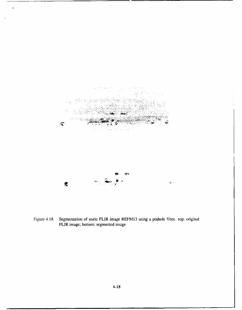
.. .. . ... . . . . ,~ " .. . i o .. ... . . .

IFigure 4.18. Segmentation of static FLIR image REFM13 using a pinhole filter, top: original

FLIR image; bottom: segmented image

4-18

4.3.4 Testing With Real-Time FUR Imagery The real-time FLIR imagery was segmented

using the same permanent circular aperture filter as was used for static FUR segmentation. A

split-screen video tape was made showing the unsegmented FLIR tape on the upper left-hand

comer of the screen and the segmented image on the upper right-hand comer of the screen.

Figure 4.19 shows the optical configuration used to observe both the segmented and unsegmented

real time FLIR images synchronously, using a beamsplitter placed just before the filter, a second

lens, a second CCD camera, and a quad input video processor. The second lens, L5 , had a

focal length of 250 mm, which was smaller than the 300 mm focal length of L4. Hence, the

unsegmented FUR image scene is shown slightly smaller than the segmented FLIR image.

In this forum, the real power of optical segmentation can be observed and appreciated,

because of its ability to perform instantaneous two-dimensional Fourier transforms. A similar

digital segmentation algorithm would be bogged down very quickly trying to calculate Fast Fourier

transforms (FFT's) and inverse FFT's at 30 frames/sec. Two digitized frames of the video (not

synchronous) are shown in Figure 4.20. Noise around the edges of the circular window was

inherent noise from the lenses and the LCTV screen. When seen in real time, these noisy bright

spots are constant and don't change (compare noise around edge in segmented FLIR image, frame

I to noise around edge in segmented FLIR image, frame 2). Further post-processing of the

segmented FLIR imagery could be accomplished to remove this constant noise factor.

4.4 Summary

This chapter presented and discussed the characterization and testing of the three types

of orientation specific, bandpass spatial filters designed and implemented in this research effort.

Pinhole pair filters implemented on heavy, black aluminum foil were demonstrated to have the

best segmentation capability out of all three filter designs. When an optimal pinhole filter was

found, it was made permanent by drilling circular apertures into aluminum squares. The Gabor

CGH filters implemented on holographic glass slides exhibited the expected intensity profiles of

odd and even gaussian pairs, but the contrasts of the emulsion on the glass slides could not be

made opaque enough to block the unwanted portions of the image spectrum. Pinhole pair filters

implemented on the LCTV had poor segmentation capability because of aliasing of the periodic

segmented images due to the low resolution of the LCTV. The low resolution of the LCTV was

4-19

w-

0

w

C.,L

U,

-J) 0

Cj0

Fig~ure 4.19. Optical setup used for observing segmented and unsegmented real time FUIRimages synchronously

4-20

Figure 4.20. Segmentation of two frames of real-time FLIR imagery using a circular aperturepair filter with two orientations, 0 and 900. top left: original FLR image, frame1; top right: segmented FUR image, frame 1; bottom left: original FUR image,frame 2; bottom right: segmented FLUR image, frame 2

4-21

also a hindrance when used as an input medium for the FLIR images. Segmentation of the FLIR

images was not as detailed as it could be because the low resolution of the LCTV limited the

separation and dilation of the filter apertures. Real-time optical segmentation of FLIR imagery

was demonstrated.

4-22

V. Conclusions and Recommendations

This chapter presents a summary of thesis results, provides conclusions based upon these

results, and bffers recommendations for future research efforts.

5.1 Summary

There were two major goals of this thesis: 1) Design and implement orientation specific,

bandpass spatial filters for use in an optical setup including Gabor filters and filters implemented

on an LCTV for real-time filter selection; 2) Test these spatial filters for their ability to segment

various input images including FLIR imagery displayed on an LCTV.

Three major filter designs were developed. The first design was simple pinhole pair filters

implemented on heavy, black aluminum foil. They were modeled as symmetrically located

circular apertu, s which correspond to Airy disc wavelets. Because of their simplicity and

flexibility, these filters were used most often in this research effort. Segmentation results using

these filters turned out to be very good with capabilities of very fine detail. However, because

of the low resolution of the LCTV, aperture dilations and separations could not be optimized for

segmenting the FLIR imagery. Optical segmentation of static and real-time FLIR imagery was

demonstrated using a simple pinhole pair filter. The second design was sine and cosine Gabor

filters implemented using detour-phase computer generated holography. The 3-D plots of the

Gabor filters showed them to have the correct characteristics of the odd and even gaussian pairs

(FT of Gabor wavelets); however, the spectrum of the Gabor filters (Gabor wavelets) showed

undesirable DC terms. Consequently, the Gabor filters designed in this thesis did not demonstrate

good segmentation capabilities because they passed too much of the image background. The final

filter design was pinhole pair filters implemented on an LCTV to investigate the ability of real-time

filter selection. The spectrums of the pinholes pairs implemented in this way produced periodic

wavelets; however, the resolution of the LCTV was not high enough to keep the segmented images

from interfering with one another.

5-1

5.2 Conclusions

An automatic, optically based image segmentation scheme for locating potential targets in a

cluttered FUR image has been implemented successfully. By using the proper choice of aperture

pair separation, dilation, and orientation, potential targets in FLIR imagery can be optically

segmented using spatial filtering techniques.

The most successful segmentation filter design was the simple pinhole pair filter (circular

aperture pairs) implemented on heavy, black aluminum foil. This design proved to be easy to

implement, highly flexible, and capable of very fine segmentation detail. Highly detailed edge

segmentation of template slides was realized in the described optical setup using simple circular

aperture pair filters with 6 mm separations, 3 mm dilations, and orientations of 30, 90, and 150'.

Gabor filters implemented with detour-phase holography and photoreduced onto holographic

glass plates were not successful segmentation filters due to the inability of the emulsion to block

the unwanted portions of the image spectrum. However, due to the success with the pinhole filters,

further pursuit of implementing Gabor filters may not be warranted.

Pinhole filters implemented on an LCTV were not successful segmentation filters in the

optical configuration used due to the low resolution of the LCTV. Since grey-scale capability is not

necessary for this implementation, the use of a higher resolution, binary SLM may be warranted.

The LCTV was successful as an input image SLM for segmentation of static and real-time

FUR imagery. Because the resolution was low, aperture separations were limited to 4 mm,

aperture dilations were limited to 2 mm, and orientations were limited to 0 and 90'. However,

because of the need for a grey-scale input medium, a higher resolution, binary SLM was not

deemed feasible for this application.

5.3 Recommendations

1) Further investigation into real-time filter selection might benefit by incorporating a higher

resolution binary SLM instead of the LCTV used in this research effort. For example, the

SEMETEX 128 x 128 iron garnet MOSLM has a resolution approximately five times better than

the LCTV (i.e., pixel spacing five times closer together), and since grey-scale is not necessary for

5-2

implementing circular aperture pairs, the binary capability would be an advantage by enhancing

the contrast.

2) Only single frequency, single dilation, multiple orientation filters were used during this

research effort, because multiple frequencies or multiple dilations were found to interfere with

one another. Lateral inhibition might be the key to getting around this problem by "running"

many different single frequency, single dilation, multiple orientation filters at the same time and

"choosing" the best correlation output of one of the filters at any given moment for higher level

processing. One way to implement lateral inhibition could be to place many single frequency,

single dilation, multiple orientation filters at duplicate Fourier planes containing the spectrum of

the input image. The duplicate Fourier planes could be made by using multiple beamsplitters

positioned in the area just before the original filter plane. Then, multiple lenses and CCD cameras

could be used to observe the correlation planes and feed the outputs into a computer. The computer

could then parallel process the multiple outputs and chose a "winning" correlation image at any

(liven moment based on, say, average pixel brightness and pass the pixel coefficients to a higher

level of processing.

5-3

Appendix A. Detour Phase Hologram Production

The following program, Gabor-Filter, generates a plotfile that can be used to producc detour

phase holograms of Gabor filters on a laser printer. Examples of Gabor filter holograms are shown

in Figures 3.5 and 3.6. The program was written in FORTRAN code in order to take advantage

of the METALIB library of plotting programs available on the UNIX system at AFIT. It's is a

modified version of a program presented in an AFIT thesis by Vicky Robinson (32:37-38) to

generate moment holograms.

This Appendix is divided into four sections. First, the program is presented; second, the

computational processes and variables of the program are explained; third, some modifications in

the Robinson program for compilation purposes are discussed; and last, methods of compiling,

previewing, plotting, and photoreducing the holograms are explained.

A.] Gabor-Filter Program

Program GABOR-FILTER

c This program generates a plot on the IMAGEN printer thatc can be used to generate a computer generated hologram ofc Gabor filters.c Written by Chris Veronin, Summer 1990c Modified from a CGH program written by Vicki Robinson

Parameter (D=64.0000)character*25 filenameInteger ntyp, nbeg, nend, norient, nangReal D, :-:, y, hmag, df, rf

Print*,'Plot filename to be created:Read (5,2000) filename

2q00 Format (alO)Print*,'Enter "0" for cosine or "1" for sine Gabor.'Read(5, *) ntypPrint*,'Beginning Order? (0,1,2,or 3)'Read (5, *) nbegPrint*,'Ending Order? (0,1,2,or 3)'Read(5,*) nend

A-I

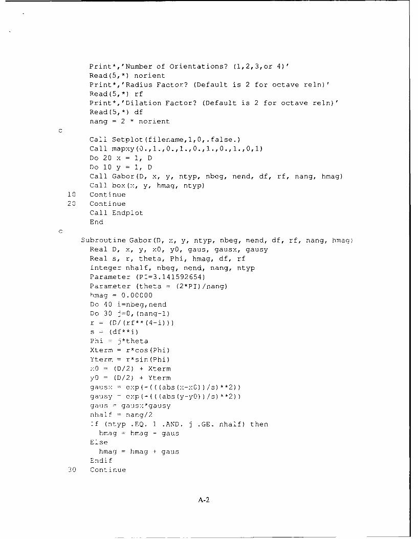
Print*,'Number of orientations? (l,2,3,or 4)'

Read (5, *) norientPrint*,'Radius Factor? (Default is 2 for octave rein)'

Read(5,*) rfPrint*,'Dilation Factor? (Default is 2 for octave rein)'Read(5,*) df

nang =2 * norient

C

Call Setplot(filename,l,0,.false.)

Call mapxy(O.,l.,.,l.,.,l.,0.,l.,0,l)Do 20 x = 1, DDo 10 y = 1, DCall Gabor(D, x, y, ntyp, nbeg, nend, df, rf, nang, hmag)Call box(x, y, hmag, ntyp)

10 Continue

20 Continue

Call Endplot

End

C

Subroutine Gabor (D, x, y, ntyp, nbeg, nend, df, rf, nang, hmag)Real D, x, y, xO, yO, gaus, gaus-:, gausy

Real s, r, theta, Phi, hrnag, df, rfInteger nhalf, nbeg, nend, nang, ntypParameter (P1=3.141592654)

Parameter (theta =(2*PI)/nang)

hmag =0.00000

Do 40 i=nbeg,nend

Do 30 j=0, (nang-l)

r =(D/(rf**(4-~i)))

s =(df**i)

Phi = j*thetaXterm = r*cos (Phi)Yterm = r*sin (Phi)

0= (D/2) + Xtermy0 = (D/2) + Yterm

gausy = e:p-(((abs(y--yO))/s)**2))

gaus =gaus:: *gausy

nhalf =nang/2

If (ntyp .EQ. 1 .AND. j .GE. nhalf) thenhmag = hmag - gaus

Else

hmag = hmag + gausEndif

30 Continue

A-2

40 ContinueReturn

End

C

Subroutine box(., y, hmag, ntyp)

Real ,:, y, hmagInteger ntyp, icx, icy, ih, ilx, ilyParameter (iboxw=35, iw=17, ihmax=35, iosx=500, iosy=90)icx = x*iboxw - (iboxw/2) + iosxicy = y*iboxw - (iboxw/2) + iosyIf (ntyp .EQ. 1) then

ih = (ihmax/2) + (ihmax/2)*hmagElse

ih = ihmax * hmag

Endifilx = icx - (iw/2)ily = icy - (ih/2)Do 50 i = ilx, ilx+iw

Call drv(i, ily, i, ily+ih)50 Continue

Return

End

A.2 Process and Variable Explanation

Essentially, the main program generates the plotfile in three steps. First, it establishes the

plotting directions to the printer by calling the METALIB subroutines Setplot and mapxy. Second,

it calls the subroutine Gabor to compute the height, hmag, of the rectangles in the hologram, one

at a time. Finally, after each height is computed, it calls the subroutine box which directs the

plotting of the rectangle using the METALIB subroutine drv. The finished plot is tie negative of

the desired filter image, because the photoreduction process reverses the contrasts.

A detailed explanation of the function Gabor is presented in the next section. Detailed

explanations of the METALIB subroutines can be found in either the METALIB manual (online

on the UNIX system) or the Robinson thesis, and a detailed explanation of the subroutine box can

be found in the Robinson thesis (32:38-41).

A-3

Sy Gaussian Region

rsin(Phi) r

Phi

(D/2,D/2) rcos(Phi) x

Figure A. 1. Location of gaussian regions in Gabor filter holograms

A.2.1 The Subroutine Gabor The subroutine Gabor computes the height of any given

rectangle in the hologram at location (x, y). The height is calculated from the following equation:

gaus = exp[-(Ix - xol/s) 2] exp[-(ly - y01/s) 21 (A.1)

where x and y indicate the location of the rectangle in the array D x D, x0 and yo indicate the

location of a gaussian region in relation to the center point of the array at (D/2, D/2), and s

indicates the dilation of the gaussian regions.

Figure A. 1 shows the radius of the frequency rings as r and the angle from the . axis as

Phi. The radius r can vary depending on the range of frequency rings input (nbeg to nend) and

the radius factor, rf. If rf is chosen to be 2, then the program varies the radius r in octave steps,

i.e., D/16, D/8, D/4 ... D/[2(4-')]. The angle Phi is determined by spacing the gaussian

pairs (# of orientations) evenly around the center point relative to the first pair at 0 and 7r radians.

The dilation s is a constant within a frequency ring and varies according to the dilation factor,

(If, and the range of the frequency rings input. If df is chosen to be 2, then s takes on values of

1. 2.4..... 2'. s is related to the standard deviation of a gaussian by a = s/ v".

A-4

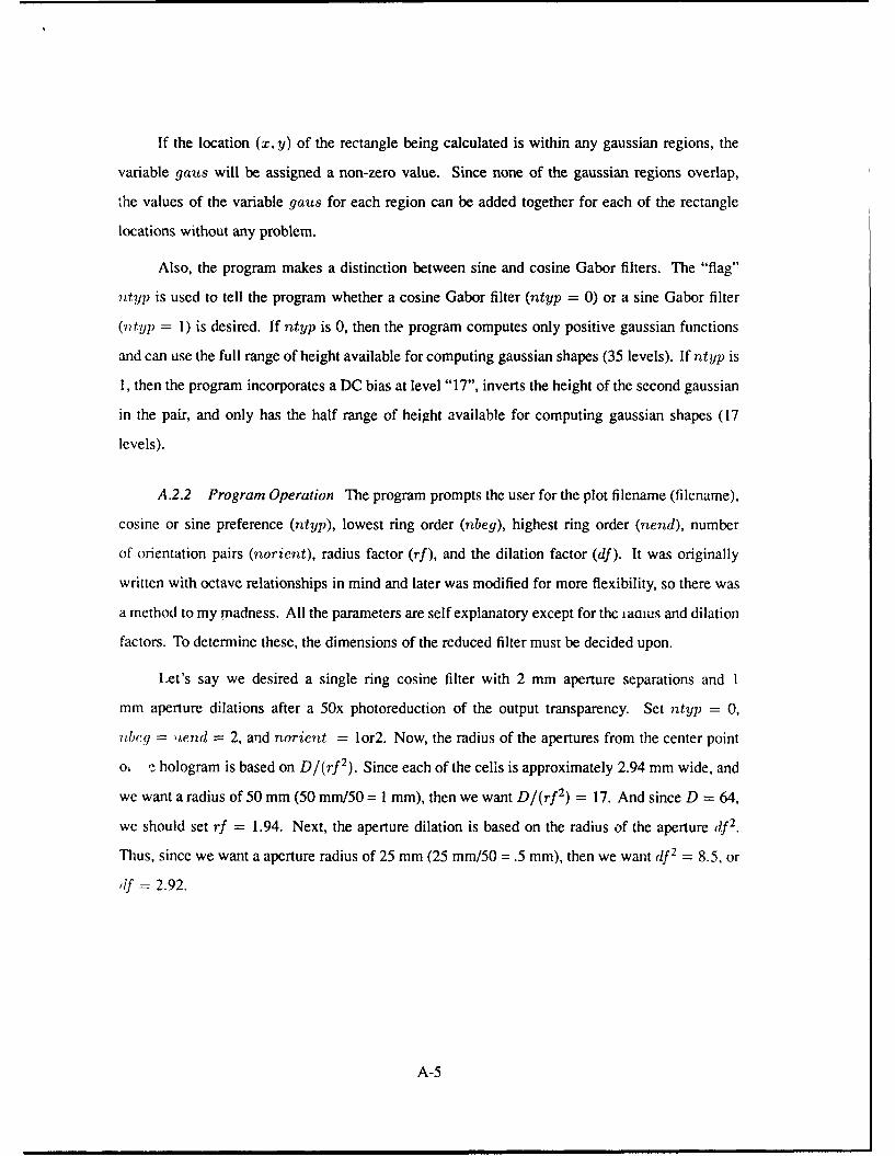
If the location (x, y) of the rectangle being calculated is within any gaussian regions, the

variable gaus will be assigned a non-zero value. Since none of the gaussian regions overlap,

.he values of the variable gaus for each region can be added together for each of the rectangle

locations without any problem.

Also, the program makes a distinction between sine and cosine Gabor filters. The "flag"

ntyp is used to tell the program whether a cosine Gabor filter (ntyp = 0) or a sine Gabor filter

(ntyp = 1) is desired. If ntyp is 0, then the program computes only positive gaussian functions

and can use the full range of height available for computing gaussian shapes (35 levels). If ntyp is

1, then the program incorporates a DC bias at level "17", inverts the height of the second gaussian

in the pair, and only has the half range of height available for computing gaussian shapes (17

levels).

A.2.2 Program Operation The program prompts the user for the plot filename (filename),

cosine or sine preference (ntyp), lowest ring order (nbeg), highest ring order (nend), number

of orientation pairs (norient), radius factor (rf), and the dilation factor (df). It was originally

written with octave relationships in mind and later was modified for more flexibility, so there was

a method to my madness. All the parameters are self explanatory except for thc iamus and dilation

factors. To determine these, the dimensions of the reduced filter must be decided upon.

Let's say we desired a single ring cosine filter with 2 mm aperture separations and 1

mm aperture dilations after a 50x photoreduction of the output transparency. Set ntyp = 0,

,nbcg= nend = 2, and norient = lor2. Now, the radius of the apertures from the center point

o, ' hologram is based on D/(rf2). Since each of the cells is approximately 2.94 mm wide, and

we want a radius of 50 mm (50 mm/50 = 1 mm), then we want D/(rf2) = 17. And since D = 64,

we should set rf = 1.94. Next, the aperture dilation is based on the radius of the aperture df 2.

Thus, since we want a aperture radius of 25 mm (25 mm/50 = .5 mm), then we want (If 2 = 8.5, or

(If = 2.92.

A-5

A.3 Compiling, Previewing, Plotting, and Photoreducing

A.3.1 Compiling To compile the program on the UNIX system at AFIT the following

command should be used:

f 77 - o programname programname.f - Imetalib (A.2)

Then, by typing the programname, the plotfile can be generated. Note: Metalib is a library

residing in the UNIX mainframes at AFIT (it does not need to be in your path). Metalib is not on

all the UNIX systems, but as of Summer 1990 it was at least on Blackbird and Galaxy.

A.3.2 Previewing Before plotting the hologram on the laser printer, it's a good idea to

preview it first on the computer screen. Especially, since the holograms take an average of 20

minutes plotting time each on the IMAGEN printer.

The plots can be previewed on the terminal by using a Tektronix 4012/4014 screen emulator

and the following command:

plot pltname - Trek (A.3)

Two Tektronix screen emulators were found to work well. One can be found on the SUN

Workstations by using the command Tektool. The other can be found on the MicroVax system

by opening a Tektronix 4012/4014 window. Clear the screen before previewing with the clear

command. Also, make sure the system environment is set for the right terminal by using the set

term = tek command.

An alternative method is to print the hologram to a file using the postscript printing command

(see next section on plotting), and then use a postscript previewer to examine the hologram. For

,xamplc, the NeXT machines in room 2011, Bldg 642, have postscript previewers that have been

ased for this purpose.

A.3.3 Plotting To make a hologram, a transparency should be used as the plotting medium.

The hologram can be plotted on an IMAGEN printer by using the mit command:

it pltnamc Ilpr - P(printcrname) (A.4)

A-6

or it can be plotted on a Postscript printer by using the mps command:

mps plItnarne Ilpr - P(printernane) (A.5)

For postscript previewing purposes, print the hologram to a file using the command:

raps plItname > pItnane.eps (A.6)

An alternative method to printing directly onto a transparency is to print the hologram on

white paper using the commands above, and then thermofax the image onto a transparency. The

advantage of this method is a darker, more uniform, and higher contrast transparency hologram.

A.3.4 Photoreducing After plotting, the transparency should be photoreduced in order to

use it in an optical imaging system. The transparencies generated in this research effort were

reduced 50x onto a 2 x 2 x .06in. glass holographic plate. This was accomplished by using a

35 mm lens in the Dekacon optical photoreduction system located in the Cooperative Electronics

Materials Processes Laboratory (room 1065) in building 125. Photoreduction procedures can be

found in the Robinson thesis (32:42-43), the Childress and Waldron thesis (9:100-103), or in the

Dekacon instruction sheets found in a 3-ring binder located with the Dekacon system.

A-7

Appendix B. LCTV Modifications and Limitations

B.I Introduction

This Appendix was written to discuss some of the details regarding the modifications, liquid

crystal display (LCD) configuration, and resolution limitations of the liquid crystal television

(LCTV) used in the optical setup as an amplitude spatial light modulator (SLM).

Over the past five years, LCTVs have been demonstrated as capable amplitude and phase

SLMs in optical image processing setups in various research projects (4, 7, 8, 14, 17, 19, 18, 20,

27, 22, 24, 25, 29, 36, 39, 40). The main advantage of LC7 -,Is is low cost (approximately $100 to

$ 1200), and their main disadvantage is low resolution (fixel sizes on the order of 370 jm). Many

researchers have overlooked the low resolution disadvantage in order to implement a low-cost

demonstration of dynamic optical image processing.

The main reason for using an LCTV in this research effort was the need for a low-cost,

gray-scale SLM in order to demonstrate real-time segmentation of input gray-scale FLIR imagery.

The LCTV chosen was a Sony Video Walkman LCTV. The television unit came equipped with a

built in 8mm video cassette recorder (VCR), video and audio input/output jacks, a battery pack

for portability, and a lot of other nice bells and whistles. It retails for about $1200. Specifications

for the LCD are given in Table B. 1. These parameters were taken from a design and specification

manual for the Sharp LCD, Reference (35). Two Sony Video Walkman LCTVs and a Sony CCD

camera were purchased for this rescarch effort through the thesis sponsor WRDC/AARI-2, POC:

Capt Kevin Ayer.

B.2 LCTV Theory

An excellent presentation of theory behind the operation of an LCTV as an amplitude SLM

for use in a coherent imaging setup can be found in Reference (23). In addition to theory, this paper

characterizes and compares the capabilities of three different LCTVs and discusses the advantages

of an active matrix using a thin-film transistor (TFT) at every pixel. Also, Ken Hughes' thesis (18)

includes a section on LCTV theory and operation as an amplitude SLM, as well as many of the

other references given at the beginning of this Appendix. For a good presentation on the theory

and operation of an LCTV used as a phase SLM, see Reference (25).

B-I

Table B. I. Mechanical Specifications of Liquid Crystal Display

Parameter Specifications UnitManufacturer SharpModel # LQ424A01Addressing method TFTDisplay format 479 (W) x 234 (H) PixelsActive area 81.9 (W) x 61.8 (H) mmScreen size (Diagonal) 4 InchPixel pitch 0.171 (W) x 0.264 (H) mmPixel configuration RGB delta configurationOutline dimensions* 110.2 (W) x 85.8 (H) x 20.7 (D) mmWeight 170±10 g" Excluding protrusions

B.3 Modifications

As much as I hated to do it, the Sony Video Walkman had to be modified before it could

be used in the optical setup. Essentially, the LCD had to be removed from its hinged case

where the backlighting florescent tubes and diffuser resided as well as many of the video and

audio electronics. Quite honestly, taking the LCTV apart and removing the LCD was a trial and

error exercise, since there was no technical manual available dealing with this kind of "repair".

However, the modification was successful. Hopefully the following description of steps taken to

remove the LCD from its case will help anyone wishing to modify the second LCTV or wishing

to put the modified LCTV back together.

B.3.1 LCTV Disassembly 1) Remove two top screws from back of hinged unit and two

bottom side screws from hinged unit (all four have arrows pointing to them) using a jewelers

screwdriver. Notice the two side screws are shorter than the top screws.

2) Remove circuit board unit by removing two medium sized upper left and lower right

screws and two upper left ribbon cables (ribbon cables slide out after snapping open holdcrs).

3) Remove florescent tubes. Note: blue and red dots were up and on the side of the LCTV

with the video/audio jacks; metal contact strips were down.

4) Remove diffuser unit by removing the four comer screws on the unit (long and finely

B-2

threaded). Also, need to remove side push-button panel used for setting the clock, etc. by

disconnecting its cable from the circuit board unit and removing the two mounting screws.

5) Diffuser unit and upper push-button panel should come out easily exposing the LCD

unit. BE CAREFUL NOT TO SCRATCH THE LCD! Place a soft cloth under the LCD unit when

laying it down.

6) Remove LCD unit from front holder and disconnect its ribbon cable from the circuit

board unit.

7) Remove SECOND diffuser plate within LCD unit by first removing the two comer screws

(silver) from back of unit and prying metal casings apart at the comers (some finesse will be

needed here).

8) After prying apart the metal casings so that diffuser plate is accessible, place the LCD

unit so the ribbon cable is oriented up and diffuser plate is exposed.

9) Carefully remove diffuser plate (it's just sitting in there).

B.3.2 LCTV Assembly 1) Put LCD unit back together without diffuser plate installed. Top

metal casing goes to outside.

2) Replace small silver screws back in their opposite comers and reconnect LCD unit ribbon

cable to circuit board unit.

3) Place a cloth around LCD unit and lay it on top of VCR unit (top of LCTV).

4) Reassemble the hinged unit in reverse order without installing LCD unit, florescent tubes,

nr side push-button panel.

13.4 LCD Configuration and Spatial Resolution Limitations

The following two subsections detail the LCD pixel configuration and spatial resolution

limitations of the Sony Video Walkman LCTV. This research was accomplished in order to figure

out the origins of the LCTV spectrum, characterize the LCTV for comparison to other SLMs, and

determine the resolution limitations of the LCD.

B-3

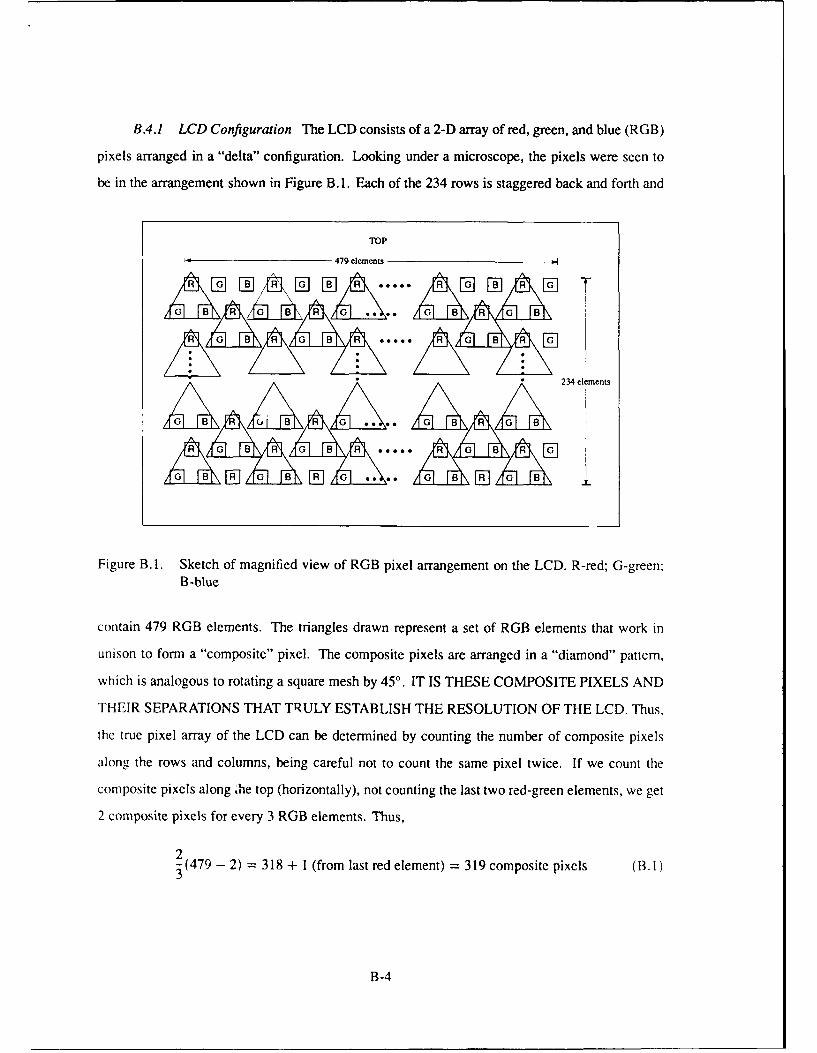
B.4.1 LCD Configuration The LCD consists of a 2-D array of red, green, and blue (RGB)

pixels arranged in a "delta" configuration. Looking under a microscope, the pixels were seen to

be in the arrangement shown in Figure B. 1. Each of the 234 rows is staggered back and forth and

TOP

19479 elemerts -IAo A

234 elements

BL F2BR G .... RIFBIJR K

AG B. ..bZ G B R G~~IJ~ B

Figure B.1. Sketch of magnified view of RGB pixel arrangement on the LCD. R-red; G-green;B-blue

contain 479 RGB elements. The triangles drawn represent a set of RGB elements that work in

unison to form a "composite" pixel. The composite pixels are arranged in a "diamond" pattern,

which is analogous to rotating a square mesh by 45O. IT IS THESE COMPOSITE PIXELS AND

THEIR SEPARATIONS THAT TRULY ESTABLISH THE RESOLUTION OF THE LCD. Thus,

the true pixel array of the LCD can be determined by counting the number of composite pixels

along the rows and columns, being careful not to count the same pixel twice. If we count the

composite pixels along ie top (horizontally), not counting the last two red-green elements, we get

2 composite pixels for every 3 RGB elements. Thus,

u(479- 2) = 318 + I (from last red element) = 319 composite pixels (B.I)

B -4

And along the side (vertically), we get I composite pixel for every 2 RGB elements. Thus,

1(234) = composite pixels-(3)=117 copst ies(B.2)2

Using these numbers, we see that the LCD has a smaller composite pixel array of approximately

319 (W) x 117 (H) than what appeared to be presented in the specifications in Table B.1 of 479

(W) x 234 (H).

Next, composite pixel spacing was calculated using the active area dimensions given in

Table B.1 and taking into account the fact that the rows are staggered, we get a horizontal

composite pixel spacing of81.9 = .257 mm (B.3)

319

and a vertical composite pixel spacing of

61.8 mm= .265 mm (B.4)233

However, because the rows are staggered, the actual composite pixel spacing is determined by

finding the hypotenuse of the horizontal and vertical components of the composite pixels, see

Figure B.2. Thus, the actual composite pixel spacing was found to be

.265 2 + .2572 = X 2 thus, x = .370 mm (B.5)

The composite pixel spacing of .370 mm is equivalent to the pixel spacing of black and white

LVTVs (23); however, the contrast of the Sharp LCD is much better due to the TFT active matrix.

B.4.2 Spatial Resolution Limitations The resolution limitations of the LCTV can be best

lemonstrated by observing its spectrum and determining the range of spatial frequencies that it

can resolve before aliasing occurs. The spectrum of the LCTV was 'rved using the optical

setup shown in Figure B.3. Ll was a 250 mm lens which was used to take the Fourier transform

of the LCTV image. L2 was a 40x microscope objective which was used to magnify the LCTV

spectrum onto the CCD camera. The spectrum of the LCTV with no input image displayed is

shown in Figure B.4.

B-5

TOP

.265

Figure B.2. Sketch showing composite pixel spacing components

IN PUT(LCTV) LI

OUTPUTL2

CCO CAMERA

VCR

FRAMEGRABBER

Figure B.3. Optical setup used to observe LCTV spectrum

B -6

Figure B.4. Spectrum of LCTV with no input image displayed

Bar patterns containing different spatial frequencies were imaged onto the LCTV screen

using a Panasonic video camera. I was found that the LCTV can resolve the spectral coefficients

from di played bar patterns containing spatial frequencies of 4 cycles/cm to 12 cycles/cm. Spectral

coefficients from spatial frequencies any lower than 4 cycles/cm vere lost in the pixel DC, soc

Figure 13.5. Spectral coefficients from spatial frequencies any higher than 12 cycles/cm began to

intcrfere with one another due to aliasing, see Figure B.6. Thus, the resolution of the L.CTV is

I:mitcd to 4 to 12 cycles/cm. No matter how much more the spectrum is magnified, this resolution

itnitatic 1 will remain fixed.

B-7

Figure B.5. Spectrum of LCTV with spectral coefficients from 4 cycle/cm bar pattern displayedshowing lower resolution limit of LCTV.

B-8

Figure B.6. Spectrum of LCTV with spectral coefficients from 12 cycle/cm bar pattern displayedshowing upper resolution limit of LCTV.

B-9

Appendix C. Barplot Generation

The following program, Barplot, generates a plotfile that was used to produce barplots of

,;arying frequencies that were, in turn, used to create texture input slides for the spatial filtering

experiments described in this thesis. The finished texture slides used are shown in Appendix D.

The program was written in FORTRAN code in order to take advantage of the METALIB library

of plotting programs available on the UNIX system at AFIT. It uses a modified version of the

subroutine box written in a program presented in an AFIT thesis by Vicky Robinson (32:37-38) to

generate moment holograms.

This Appendix is divided into three sections. First, the program is presented; second,

the computational processes ind variables of the program are explained; and last, methods of

compiling, previewing, plotting, and photoreducing the holograms are explained.

C. I Barplot Program

Program BARPLOT

C

c Program for plotting textured imagesc Written by Chris Veronin

character*25 filenameinteger cycles

write (6,1000) "Plot filename to be created:1000 format (a31)

read (5,2000) filename2000 format (al0)

write (6,3000) "Number of cycles/cm:3000 format (a23)

read (5,4000) cycles4000 format (i4)

Call Setplot(filename,1,0,.false.)Call map:y(0.,I.,l.,I.,0., ., .,,I.,0,l)Do 30 m = 1, cyclesDo 20 n = 1, cycleshmag = 1.0

C-I

Call bo:-(cycles,m,n,hmag)20 Continue

30 Continue

Call EndplotStop

End

C

Subroutine box (cycles,m, n,hmag)

integer cycles

iboxw = (2560 - 25)/cycles

ihma.:: = ibo.:wiw = ibo-':w/2

ios:-: = ((3328 - (cycles * iboxw)) + 30)/2iosy = ((2560 - (cycles * ihmax)) + 25)/2ic: = m*ibo:.:w - (iboxw/2) + ios::

icy = n*iboxw - (iboxw/2) + iosyih = ihmax * hmagil: = ic - (iw/2)ily = icy - (ih/2)

Do 10 i = il.:,il,- + iwCall drv(i,ily,i,ily+ih)

10 Continue

Return

End

C.2 Explanation of Program

The program is basically a very scaled-down version of the GaborFilter program presented

in Appendix A, i.e., make use of what you've got. However, instead of computing the different

heights of the cell rectangles, this program sets all the heights to 1.0 and divides the widths of the

rectangles into equal values depending on the number of cycles entered at the program prompt.

The subroutine box is modified slightly in order to take full advantage of the pixel dimensions

for an entire sheet of paper for the IMAGEN printer (3328 x 2560 instead of 3270 x 2445 as

cited in the Robinson thesis). Detailed explanations of the METALIB subroutines can be found

in either the METALIB manual (online on the UNIX system) or the Robinson thesis, and a

more detailed explanation of the subroutine box and its parameters can be found in the Robinson

thesis (32:38-41).

C-2

C.3 Output Procedures

The previewing, plotting, and photoreduction procedures are the same here as they were for

the Gabor CGHs. One difference is that the texture slides shown in Appendix D could not made

directly from these barplots; thcy had tG be cut-out axxO pasted together, and then transferred to

transparencies and photoreduced. The transparencies were photoreduced 20x using the 3in. Wray

lens. This produced glass slides with images approximately 1 cm square. Hence, a 10 cycle/sheet

transparency reduced 20x would produce a 10 cycle/cm input texture slide.

C-3

Appendix D. Texture Plots

This Appendix presents four different texture slides made using the barplot program

described in Appendix C and a little extra "cut and paste".

D-1

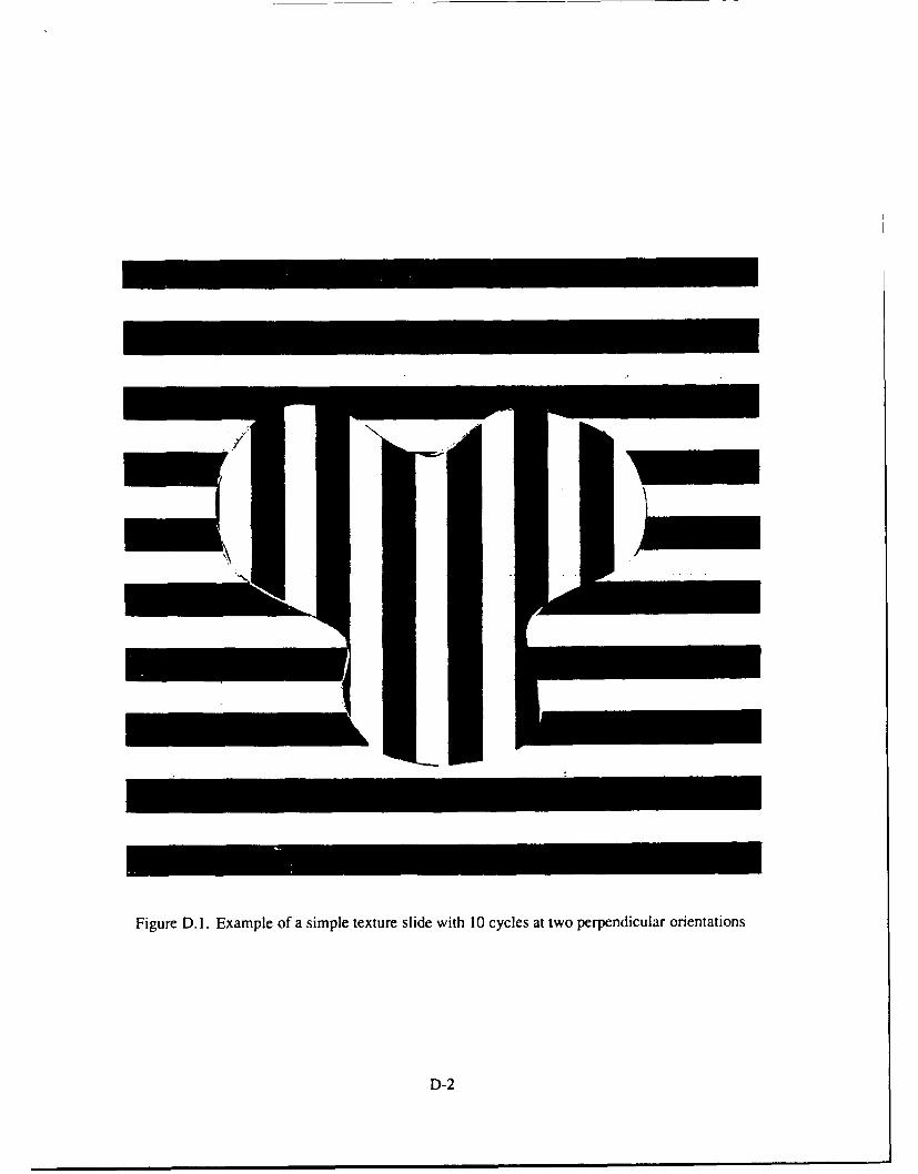
Figure D. 1. Example of a simple texture slide with 10 cycles at two perpendicular orientations

D-2

Figure D.2. Example of a simple texture slide with a 10 cycle background and two 20 cycletextures in parallel and perpendicular orientations

D-3

IIII 1I I

m

Figure D.3. Example of a more complex simple texture slide with a 10 cycle background andthree other textures consisting of 30, 40, and 50 cycles at 0, 45, 90, and 135'orientations

D-4

Figure D.4. Example of a more complex simple texture slide with a 10 cycle background andfour other textures consisting of a 20 cycle center texture and 30, 40, and 50 cycleouter lobes, all at different orientations

D-5

Bibliography

1. AT&T. Truevision Advanced Raster Graphics Adapter: TARGA 8, M8, 16, 24, and 32,User's Guide, 1985. Release 1.1.

2. AT&T. Truevision Advanced Raster Graphics Adapter: TARGA 8, M8, 16, 24, and 32,Software Tools Notebook, 1986. Release 3.0.

3. Ayer, Captain Kevin W. Gabor Transforms for Forward Looking InfraRed Image Segmen-tation. MS thesis, AFIT/GE/ENG/89D-1, School of Engineering, Air Force Institute ofTechnology (AU), Wright-Patterson AFB OH, December 1989 (AD-A215046).

4. Barnes, Thomas H., et al. "Phase-only modulation using a twisted nematic liquid crystaltelevision," Applied Optics, 28(22):4845-4852 (November 1989).

5. Bovik, Alan Conrad, et al. "Multichannel Texture Analysis Using Localized Spatial Filters,"IEEE Transactions on Pa:tern Analysis and Machine Intelligence, 12(1):55-73 (January1990).

6. Bush, Captain Larry F. The Design of an Optimum Alphanumeric Symbol Set for CockpitDisplays. MS thesis, AFIT/GE/EE/77-1 1, School of Engineering, Air Force Institute ofTechnology (AU), Wright-Patterson AFB OH, December 1977 (AD-A053447).

7. Casasent, David, et al. "Real-time deformation invariant optical pattern recognition usingcoordinate transformations," Applied Optics, 26(5):938-942 (March 1987).

8. Cheng, Yih-Shyang and Jiunn-Yann Lin. "Experimental use of a low cost liquid crystal TVin multiplex holography," Applied- -tics, 28(5):829-830 (March 1989).

9. Childress, Timothy G. and J. Thomas Walrond. Position, Scale, and Rotation Invari-ant Optical Pattern Recognition For Target Extraction and Identification. MS thesis,AFIT/GE/ENG/88D-4, School of Engineering, Air Force Institute of Technology (AU),Wright-Patterson AFB OH, December 1988.

10. Cline, Captain John D. Hybrid Optical/Digital Architecture for Distortion Invariant PatternRecognition. MS thesis, AFIT/GEO/ENG/89D-02, School of Engineering, Air Force Instituteof Technology (AU), Wright-Patterson AFB OH, December 1989 (AD-867524).

11. Daugman, John G. "Complete Discrete 2-D Gabor Transforms by Neural Networks forImage Analysis and Compression," IEEE Transactions on Acoustics, Speech, and SignalProcessing, 36(7):1169-1179 (July 1988).

12. Gaskill, J. D. Linear Systems, Fourier Transforms, and Optics. New York: John Wiley &Sons, 1978.

13. Goodman, J. W. Introduction to Fourier Optics. New York: McGraw-Hill Book Company,1968.

14. Gregory, Don A. "Real-time pattern recognition using a modified liquid crystal television ina coherent optical correlator," Applied Optics, 25(4):467-469 (February 1986).

BIB-I

15. Hamadani, Naser A. Automatic Target Cueing in IR Imagery. MS thesis, School ofEngineering, Air Force Institute of Technology (AU), Wright-Patterson AFB OH, December1981 (AD-A 115480).

16. Horev, Moshe. Picture Correlation Model for Automatic Machine Recognition. MS thesis,School of Engineering, Air Force Institute of Technology (AU), Wright-Patterson AFB OH,December 1980.

17. Hudson, Tracy D., et al. "Real time optical correlator architectures using a deformable mirrorspatial light modulator," Applied Optics, 28(22):4853-4860 (November 1989).

18. Hughes, Kenneth D. Suitability and Applications of Liquid Crystal Televisions In OpticalPre-processors. MS thesis, AFIT/GE/ENG/86D-6, School of Engineering, Air Force Instituteof Technology (AU), Wright-Patterson AFB OH, December 1986 (AD-A177603).

19. Hughes, Kenneth D., et al. "Optical preprocessing using liquid crystal televisions," AppliedOptics, 26(6):1042-144 (March 1987).

20. Jutamulia, S., et al. "Real-time noncoherent correlator using liquid crystal television,"Optical Communications, 64(2):1 15-119 (October 1987).

21. Lee, Wai-Hon. "Computer-Generated Holograms: Techniques and Applications." In Wolf,E., editor, Progress in Optics XVI, chapter III, New York: North-Holland PublishingCompany, 1978.

22. Li, Yao, et al. "Liquid crystal TV-based white light optical tracking novelty filter," AppliedOptics, 28(22):4861-4864 (November 1989).

23. Liu, Hua-Kuang and Tien-Hsin Chao. "Liquid crystal television spatial light modulators,"Applied Optics, 28(22):4772-4780 (November 1989).

24. Liu, Hua-Kuang, et al. "Optical-data-processing properties of a liquid-crystal televisionspatial light modulator," Optics Levers, I0(12):635-637 (December 1985).

25. Lu, Kanghua and Bahaa E. A. Saleh. "Theory and design of the liquid crystal TV as anoptical spatial light modulator," Optical Engineering, 29(3):240-246 (March 1990).

26. Mills, Lt Col James P. Personal interview. AFIT, WPAFB OH, 20 May 1990.

27. Mok, Fai, et al. "Real-time computer-generated hologram by means of liquid-crystaltelevision spatial light modulator," Optics Letters, I1(11):748-750 (November 1986).

28. Mueller, Captain Michael R. Investigation of Gabor Filters for Use in Reverse EngineeringVLSI Circuits. MS thesis, AFIT/GE/ENG/89D-35, School of Engineering, Air Force Instituteof Technology (AU), Wright-Patterson AFB OH, December 1989 (AD-B 138982L).

29. Perez, 0. and M. A. Karim. "An efficient implementation of joint Fourier transformcorrelation using a modified LCTV," Microwave and Optical Technology Letters, 2(6):193-196 (June 1989).

30. Perez, Osvaldo. Personal interview., ASD/ENAML, WPAFB, OH, 8 August 1990.

31. Roberts, Richard E., et al. "Three Dimensional Scene Analysis Using Stereo Based Imaging."In Proceedings of the SPIE Sixth Annual Conference on Applications ofArtificial Intelligence.Volume 937, pages 280-286, Bellingham, WA: SPIE Press, 1988.

BIB-2

32. Robinson, Capt Vicky L. Hybrid Calculation of Invariant Moments. MS thesis,AFIT/GEO/ENG/88D-3, School of Engineering, Air Force Institute of Technology (AU),Wright-Patterson AFB OH, December 1988 (AD-A158802).

33. Roggemann, Captain Michael C. Multiple Sensor Fusion for Detecting Targets in FLIR andRange Images. PhD dissertation, School of Engineering, Air Force Institute of Technology(AU), Wright-Patterson AFB OH, June 1989 (AD-A207577).

34. Ruck, Captain Dennis W., et al. "Multisensor Target Detection and Classification." InProceedings of the SPIE Conference on Infrared Sensors and Sensor Fusion, Volume 9341,pages 14-21, Bellingham, WA: SPIE Press, 1988.

35. Sharp - Electronics Components Group. Device Specification For TFT-LCD Module -ModelNo. LQ424AOI (TENTATIVE), September 1989.

36. Tam, Eddy C., et al. "Autonomous real-time object tracking with an adaptive joint transformcorrelator," Optical Engineering, 29(4):314-320 (April 1990).

37. Tong, Captain Carl Tong, et al. "Multisensor Data Fusion of Laser and Forward LookingInfrared (FLIR) foi" Target Segmentation and Enhancement." In Proceedings of the SPIEConference on Infrared Sensors and Sensor Fusion, Volume 782, pages 10-19, Bellingham,WA: SPIE Press, 1987.

38. Turner, M. R. "Texture Discrimination by Gabor Functions," Biological Cybernetics,55:71-82 (1986).

39. Yu, Francis T. S., et al. "Adaptive real-time pattem recognition using a liquid crystal TVbased joint transform correlator," Applied Optics, 26(8): 1370-1372 (April 1987).

40. Yu, Francis T. S., et al. "Multiple channel optical correlator via rotating grating on LCTV,"Applied Optics, 27(18):3770-3772 (September 1988).

BIB-3

Vita

Captain Christopher P. Vero " " He

graduated from Sahuaro High School in Tucson, Arizona in 1978 and attended Arizona State

University (ASU) in Tempe, Arizona where he received the degree of Bachelor of Science in

Electrical Engineering in May 1984. During his last year at ASU, he was accepted into the

College Senior Engineering Program of the United States Air Force and upon graduation received

his commission from Officer Training School in August 1984. His first assignment was to

the Foreign Technology Division at Wright-Patterson AFB, OH, where he served as a Foreign

Telecommunications Analyst, Command, Control, and Communications Division until entering

the School of Engineering, Air Force Institute of Technology in May 1989.

VITA-!

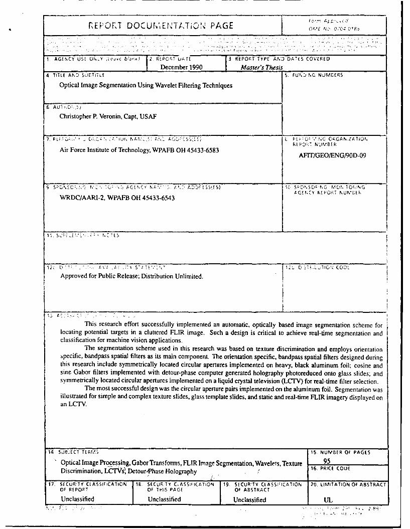
REPORT DOC"Urv' Jt,.ATi~tN, PAGE I P~ C 24O~

1. AGENCY USE 0N.Y Leavt- b/ank) 2.REPORT LDA.TE 3. REPORT TYPE AND DATES COVERED

I December 1990 Master's Thesis _______________

4 TITLE AND SUFTI'iLES.FNNGJMEZ

Optical Image Segmentation Using Wavelet Filtering Techniques

6 ALI-.C.

Christopher P. Veronin, Capt, USAF

7. FEK':. C.. ;' L ;'7'hjr, NAr.>c; AO.L AUSS" S L FE; -O .',IG ORGANiZATIOF.REPO-.T NUMIBER

Air Force Institute of Technology, WPAFB OH 45433-6583 AFIT/GEO/ENG90D-09

S 5'DNSC)--' ACE MY N47. ,. 112A~ SSE)l SP'.NSOrNG MC;?, iOFYNG

WRDC/AARI-2, WPAFB3 OH 45433-6543

12 D ,- .VT , U~~ ID 1T 0 .TC, COZC

Approved for Public Release; Distribution Unlimited.

This research effort successfully implemented an automatic, optically based image segmentation scheme forlocating potential targets in a cluttered FLIR image. Such a design is critical to achieve real-time segmentation andclassification for machine vision applications.

The segmentation scheme used in this research was based on texture discrimination and employs orientationspecific, bandpass spatial filters as its main component. The orientation specific, bandpass spatial filters designed duringthis research include symmetrically located circular apertures implemented on heavy, black aluminum foil; cosine andsine Gabor filters implemented with detour-phase computer generated holography photoreduced onto glass slides; andsymmetrically located circular apertures implemented on a liquid crystal television (LCTV) for real-time filter selection.

The most successful design was the circular aperture pairs implemented on the aluminum foil. Segmentation wasillustrated for simple and complex texture slides, glass template slides, and static and real-time FLIR imagery displayed onan LCTV.

14 SJBIECT TERM.S 15. NUMBER OF PAGES

Optical Image Processing, Gabor Transforms, FLIR Image Segmentation, Wavelets, Texture 9Discrimination, LCTVs, Detour-Phase Holography 1.PIECD

17. SECUR'TY CLASSIFICATION 18, SECUR TY CLASSIFICATION 19. SECURITY CLASSIFICATION 20. LIMITATION OF ABSTRACTOF REPORT OF THIS PAGE OF ABSTRACT

Unclassified Unclassified Unclassified UL

- ' . :, 2S