AW Marine Futures: BENTHIC MODELLING AND MAPPING...

Marine Futures Mapping the Benthos

1

WA Marine Futures:

BENTHIC MODELLING AND MAPPING FINAL REPORT

Ben Radford

Kimberly P. Van Niel

Karen Holmes

The University of Western Australia

June 2008

WA Marine Futures Final Report: Mapping Marine Benthos

2

EXECUTIVE SUMMARY Maps and models of the marine benthos provide the first full coverage information on basic

seafloor physical properties and deep-water biology for sections of the Abrolhos Islands,

Jurien Bay, Rottnest Island, Geographe Bay, Cape Naturaliste, Broke Inlet, Albany, Point

Anne, and East Middle Island, Western Australia. These maps provide information for

natural resource management, such as identifying potential habitat for invasive species or

areas sensitive to physical and chemical disturbance. The maps are also used for survey

sampling planning and habitat studies of mobile biota (eg fish) and fine scale sessile biota by

the Biodiversity team (WAMF), as well as providing a basis for planning for biological

baseline development and monitoring (eg WAMSI Node 4).

The first region surveyed was conducted in March and April 2006 (Cape Naturaliste), with

the final site mapping was completed in February 2008 (Broke Inlet). For all sites, continuous

coverage bathymetry and substrate texture maps were produced. Underwater tow video

footage was then collected, the imagery analysed and a database constructed of substrate and

biological benthos characteristics for habitat modelling and mapping. Substrate and

biological categories were modelled using Classification and Regression Trees (CARTS) and

data derived from the hydroacoustic surveys to predict substrate and biology in areas with no

observations.

Basic maps of substrate composition (reef, sediment) and sessile biota (vegetation, sessile

invertebrates) presence and extent were created, facilitating regional comparisons along the

southwest coast of Western Australia. These maps were used to develop sampling plans for

Baited Remove Underwater Video cameras (BRUVS) for fish surveys, drop video transect

data for detailed marine benthic biota studies (WAMF projects), and benthos trawls (WA

Fisheries). For each area, all identified benthos classes with sufficient numbers of

observations for modelling were mapped, including sediment texture and relief, reef

structures, vegetation types, and different classes of sessile invertebrates. Due to site

differences, not all classes were mapped at all field sites. The layout of video transects,

complexity of the benthos, and clarity of the imagery influenced the accuracy and

completeness of the video observations, and hence model and map accuracy.

The mapping prediction accuracy is reported, providing map users with a guideline for

interpreting the attribute reliability of the final maps. The statistical modelling and predictive

mapping approach developed for this project provide an objective, quantitative alternative to


3

traditional manually delineated marine habitat maps, and support detailed analysis of related

marine biota.


4

Contents WA Marine Futures: ........................................................................................................ 1 BENTHIC MODELLING AND MAPPING FINAL REPORT......... .......................... 1 EXECUTIVE SUMMARY .............................................................................................. 2 INDEX OF TABLES AND FIGURES............................................................................ 5 Tables.................................................................................................................................. 5 Figures................................................................................................................................. 5 1 INTRODUCTION......................................................................................................... 6 2 MAPPING METHODS................................................................................................ 7

2.1 PREPARATION OF SECONDARY DATASETS............................................7 2.2 TOW VIDEO OBSERVATIONS.......................................................................9 2.3 CLASSIFICATION TREE MODELLING AND SPATIAL EXTENSION....13 2.4 MAPS................................................................................................................14

3 SAMPLING PLANNING FOR OTHER BIOTA............... ..................................... 16 3.1 GOALS of SAMPLING PLANNING..............................................................16 3.2 SAMPLING PLANNING PROCEDURE........................................................17

4 RESULTS .................................................................................................................... 20 4.1 TOWED VIDEO SAMPLING .........................................................................20 4.2 MODEL DEVELOPMENT..............................................................................23 4.3 MODEL OUTCOMES .....................................................................................24 4.4 SAMPLING PLAN OUTCOMES....................................................................32

5. DISCUSSION AND RECOMMENDATIONS........................................................ 34 5.1 MAP APPLICATIONS AND INTERPRETATION........................................36 5.2 OUTCOME ISSUES AND SUGGESTIONS ..................................................37

6. CONCLUSION .......................................................................................................... 38 ACKNOWLEDGEMENTS ........................................................................................... 40 REFERENCES................................................................................................................ 41


5

INDEX OF TABLES AND FIGURES

Tables Table 1. Comparison of model accuracy for continuous/transition verses point based methods of video classification for the Northern Subset of the Rottenest Island tow video transects..............................................................................................................12 Table 2. Study area extents and towed video coverage ...............................................20 Table 3. Summary of towed video observations across all field sites. ........................21 Table 4. Example of accuracy reporting (Broke Inlet) ................................................24 Table 5. Assessment of substrate models across all field sites. ...................................25 Table 6. Assessment of biota models across all field sites. ........................................27 Table 7. Total area of major biotic and substrate benthos across all field sites...........30

Figures Figure 1. Example of towed video sampling plan protocol (Cape Naturaliste).............8 Figure 2. Data entry form developed in Excel VBA for segment observations based on the tow video footage (a) based on individual observations every five seconds and (b) based on recording transition points.......................................................................11 Figure 3. Example of BRUVS sampling planning procedure: Cape Naturaliste.........18 Figure 4. Example map of BRUVS sampling protocol (Cape Naturaliste).................19 Figure 5. Example of CART model prediction of kelp (Ecklonia) at the West Coast Capes. The major drivers are depth and spatial measures such as Moran’s I that indicate reef rugosity....................................................................................................23 Figure 6. Maps of probability of presence and presence/absence for one class (reef at Geographe Bay). ..........................................................................................................28 Figure 7. Combined biotic and substrate benthos maps (Broke Inlet).........................29 Figure 8. Example of completed drop camera (a) and trawl (b) sampling plans. Study site is Pt Anne. .............................................................................................................32 Figure 9. Example of completed BRUVs sampling plan overlaid on detailed substrate (a) and detailed biota (b) habitat maps. Study site is Broke Inlet. ...............................33


6

1 INTRODUCTION Maps and models of the marine benthos provide the first available information on basic

seafloor physical properties and deep-water biology for sections of the Abrolhos Islands,

Jurien Bay, Rottnest Island, Geographe Bay, Cape Naturaliste, Broke Inlet, Albany, Point

Anne, and East Middle Island, Western Australia. These maps will supply information for

assessment of the presence and extent of marine habitats, and will be used for planning and

execution of natural resource condition monitoring.

The Marine Futures project was designed to benchmark the current status of key Western

Australian marine ecosystems, and establish resource condition indicators for Natural

Resource Management (NRM) units. Across the 9 study areas approximately 14,000 kms of

the seafloor in water deeper than 10 metres have been surveyed with hydroacoustics using a

Reson 8101 Multibeam. These data were processed to construct full coverage maps of

bathymetry and textural information. Underwater tow video footage has been collected over

more than 210 linear kms. The full coverage hydroacoustic maps and observations recorded

from video footage were combined in a statistical modelling framework to produce the most

efficient, objective, and ecologically meaningful maps of sea floor features and inhabitants as

possible. The mapping method, predictive spatial modelling applied within a GIS, was

chosen as the most appropriate technique for bridging the divide between high resolution

quantitative geophysical information and qualitative video observations of substrate

composition and the vegetation and organisms visible on the seafloor. It is used to produce

detailed maps of the seafloor for natural resource management and planning.

Basic maps of substrate composition (reef, sediment) and sessile biota (vegetation, sessile

invertebrates) presence were developed which facilitate regional comparisons across the

diverse southwest coast of Western Australian waters and beyond. All identified benthos

classes with sufficient numbers of observations for statistical modelling were mapped,

including sediment texture and relief, reef structures, vegetation types, and sessile

invertebrates. The layout of video transects, complexity of the benthos, and clarity of the

imagery influenced the accuracy and completeness of the video observations, and hence

model and map accuracy.

The modelling prediction accuracy is reported. This provides map users a guideline for

interpreting the attribute reliability of the final maps. The statistical modelling and predictive

mapping approach developed for this project is an objective, quantitative alternative to

traditional manually delineated marine habitat maps. These maps are intended to support


7

biological observation, sampling, and monitoring activities for assessment of natural resource

condition by Natural Resource Management Councils.

Presented here is an overview of the predictive modelling approach to seafloor mapping,

followed by example maps and modelling results from the nine study regions. Finally, the

sampling planning process for the Biodiversity projects (fish, and benthic biology drop

cameras and trawls) are explained and demonstrated.

2 MAPPING METHODS The predictive modelling approach consists of three main components following the

hydroacoustic surveys and video footage collection:

(1) Data preparation:

a. Development of secondary datasets from the hydroacoustic data that provide

unique textural information about the seafloor;

b. Design and execution of a video analysis plan for modelling; these

observations are the primary data identifying the seafloor substrate and

biological features;

(2) Modelling: Model development for all substrate and biological categories as a

function of bathymetry and derived datasets to provide a framework for predicting

values in areas where no observations are available;

(3) Mapping: Application of the models to all areas surveyed with hydroacoustics to

predict the most likely substrate and biological features in locations where no field

observations (video data) were available, creating full coverage maps.

2.1 PREPARATION OF SECONDARY DATASETS The bathymetry and backscatter datasets (2.5-m pixel size) derived from the hydroacoustic

surveys (Fugro Pty Ltd) constituted the core full-coverage datasets for modelling the spatial

distribution of seafloor characteristics and for producing habitat maps. The bathymetry data

were used to develop a variety of textural datasets (see Table 1). This involved applying

algorithms to the bathymetry data using “moving window” kernels (5, 10, 25 and 50 cell

radius circles) to reveal textural differences. The algorithms calculate the relationship

between the central cell and its neighbours within the kernel, and were run for every cell in

the bathymetry grid.

These secondary datasets were used to develop a sampling plan for the towed video

observations. Towed video planning was designed based on covering the range of values of

depth as well as other secondary derivatives (eg. slope, aspect) to ensure as many unique


8

habitats as possible were sampled. Towed video plans designated primary and secondary

priority lines, allowing field crews to make decisions in regards to the weather and time

limitations.

Figure 1. Example of towed video sampling plan protocol (Cape Naturaliste).


9

2.2 TOW VIDEO OBSERVATIONS Observations of the seafloor were made of the video footage by a group of trained analysts.

Two different methods were used for analysing the towed video observations, as described

below.

METHOD 1. Cape Naturaliste, Geographe Bay, Jurien Bay, Rottnest Island (North)

The video footage was sampled at point locations to provide georeferenced point data for

modelling (Figure 2a). This required careful planning to avoid spatial autocorrelation

between the modelling data and the validation data which might inflate model goodness of fit

statistics, making the models appear better than they actually were. Spatial dependence in the

video footage within major classes was evaluated at 5 different sites, one in Western Australia

and 4 in Victoria. These revealed that vegetation was autocorrelated to a distance of

approximately 40 – 50 m, sessile invertebrates were variable, and physical characteristics all

showed a strong regional trend. Where a trend is present, there is no way to avoid spatial

autocorrelation in sampling. A distance of 50 m was selected as the minimum distance

between any of the validation data and the data used for modelling to avoid the effects of

spatial autocorrelation for the majority of the biota classes, and potentially for the sessile

invertebrate classes as well. This required the following steps:

(1) Video frames were selected that were at least 50 m apart;

(2) 25% of these were randomly selected for the validation dataset;

(3) The remaining points were assigned to the modelling dataset.

If this resulted in too few samples for modelling or validation, the percentage of the

points allocated to the validation dataset was increased, then additional points were

randomly selected from the full dataset (not requiring the 50-m spacing) for

modelling. The distance of 50 m was preserved around validation data, but not for the

modelling dataset. However, given the prohibitively high number of points in the full

dataset (typically more than 60,000), the footage was subsampled prior to modelling.

METHOD 2. Jurien Bay, Rottnest Island (North), Abrolhos Islands, Broke Inlet, Mt

Gardner, Point Anne, and East Middle Island

The video footage sampling in Method 1 was onerous, so a new, simpler methodology

(Method 2) was trialled at Jurien Bay and Rottnest Island (North). The new method was

trialled along with Method 1 to determine if the video sampling process could be streamlined.

The new method was trialled mainly due to short timelines for the project and the slow

process of video interpretation using Method 1. Instead of interpreting a number of video


10

point samples, changes in major classes of substrate and biota were identified, with all

sampling points between given the same values. This method thus identifies the transitions

from one substrate to another or one biota to another, which proved to be much faster for

video interpretation (more than four times faster).

Short segments of tape were characterised based on primary and secondary substrate qualities,

and the sessile biota present (Figure 2b). Segment length ranged from 6 seconds (the shortest

distance that can be resolved given positioning error) to several minutes. The general class of

biota (e.g. Macroalgae, seagrass) was recorded as dominant or secondary, and all individuals

identifiable within the class (e.g. Posidonia, Pyura) were noted for the segment. Dominance

was determined by the “one half rule” – if two classes are present, and the least dense class

was at least half as dense as the most dense class, both were recorded as dominant. If the

least dense class was less than half as dense as the most dense class, it was recorded as

secondary.

METHOD COMPARISON

To test the impact of changing video interpretation methods, two sites were assessed using

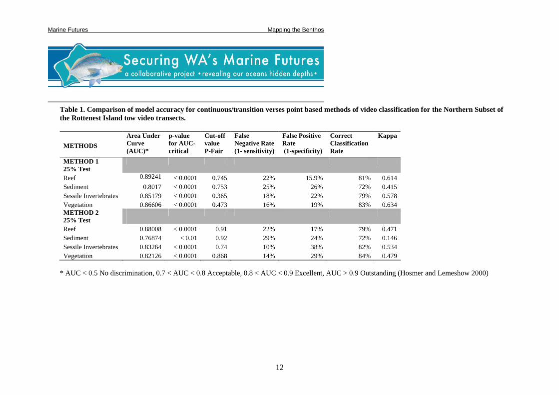
both methods. Table 2 shows the comparison of model accuracy based on both methods for

major biota and substrate classes using the northern subset of the Rottnest Island towed video

observations. Although some kappa accuracy is lost in using Method 2, the sensitivity and

specificity show that the results are actually mixed, and it is likely that little difference

between the models will be observed in final outcomes. Given the greater outcomes in terms

of speed and cost, it was decided to complete all other field sites using Method 2.


11

(a)

(b)

Figure 2. Data entry form developed in Excel VBA for segment observations based on the tow video footage (a) based on individual observations every five seconds and (b) based on recording transition points.


12

Table 1. Comparison of model accuracy for continuous/transition verses point based methods of video classification for the Northern Subset of the Rottenest Island tow video transects.

METHODS

Area Under Curve (AUC)*

p-value for AUC- critical

Cut-off value P-Fair

False Negative Rate (1- sensitivity)

False Positive Rate (1-specificity)

Correct Classification Rate

Kappa

METHOD 1 25% Test

Reef 0.89241 < 0.0001 0.745 22% 15.9% 81% 0.614 Sediment 0.8017 < 0.0001 0.753 25% 26% 72% 0.415 Sessile Invertebrates 0.85179 < 0.0001 0.365 18% 22% 79% 0.578 Vegetation 0.86606 < 0.0001 0.473 16% 19% 83% 0.634 METHOD 2 25% Test

Reef 0.88008 < 0.0001 0.91 22% 17% 79% 0.471 Sediment 0.76874 < 0.01 0.92 29% 24% 72% 0.146 Sessile Invertebrates 0.83264 < 0.0001 0.74 10% 38% 82% 0.534 Vegetation 0.82126 < 0.0001 0.868 14% 29% 84% 0.479

* AUC < 0.5 No discrimination, 0.7 < AUC < 0.8 Acceptable, 0.8 < AUC < 0.9 Excellent, AUC > 0.9 Outstanding (Hosmer and Lemeshow 2000)


13

2.3 CLASSIFICATION TREE MODELLING AND SPATIAL EXTENSION Exhaustive sampling over large areas is prohibitively expensive, and generally unfeasible. To

infer distributions of marine features from discontinuous video transect information, we need

to sample environmental relationships in detail using the combination of video footage and

the hydroacoustic surveys. This static snapshot of relationships between the observed

features we want to map from video and the spatially extensive hydroacoustic datasets helps

predict seafloor distributions from the hydroacoustics alone. This process is predictive

modelling. Video observations provide the basic information detailing what is actually found

on the seafloor, while bathymetry and textural datasets provide information on environmental

characteristics, and give full coverage of the field area. Observations are reported for all

benthic classes that are possible to identify from video (Figure 2), and their relationships with

environmental characteristics are defined through statistical modelling to predict the

probability of class presence or absence at unsurveyed locations.

The relationships between the video observations and the bathymetry-derived datasets were

characterised using classification and regression tree modelling (CART) (Breiman et al.,

1984). Classification trees are well suited to dealing with complex ecological datasets that

contain correlated predictor variables and display non-linear relationships. A detailed

description of the application of this method with marine ecological data is outlined in De’ath

and Fabricius (2000). The final trees were constructed based on the results of ten-fold cross

validation, which was used to determine the optimal tree size and to prevent over-fitting. This

ensured that the model was representative of the area as a whole, and was not biased toward

any particular subset of data. Plots of tree size (number of branches) versus classification

error were used to select an appropriate tree size (Breiman at al., 1984). S-plus and the

library “tree” were used for tree construction and graphics (Version 6.2 (2003) Insightful

Corp).

Models are simplifications of complex real world systems and must be validated, ideally with

independent data collection, or if this is not possible, with statistical methods. In this case, the

CARTs were evaluated using a subset of the video observations reserved prior to modelling

(25% of the full dataset). Specifically, the model accuracy was assessed by predicting the


14

values of the blind validation dataset and analysing the performance using ROC (receiver-

operator characteristics) analysis. ROC are commonly visualised as plots of model sensitivity

(classification accuracy) versus specificity (false positive rate). The larger the area under the

curve (AUC), the more robust the model for prediction. Models with AUC greater than 0.8

have high predictive power, values between 0.7 and 0.8 are acceptable and models with AUC

of 0.5 or less have no power of discrimination (Hosmer and Lemeshow 2000).

The probability maps (values ranging between 0.0 to 1.0) were simplified to binary

presence/absence maps (values equal to 0 or 1) for mapping. The threshold used to produce

the binary maps was determined statistically using ROC. The probability value (P) used as a

threshold was determined to avoid extreme over- or under-prediction (P-fair). P-Fair

provides a good balance between false presence, false absence, and model accuracy

particularly when the numbers of true presence values in a dataset are small. However, in the

case where a large number of true presence values are recorded, the P-Kappa value provides a

more balanced cutoff value for presence / absence values. Model evaluation and

determination of thresholds for creating binary maps were conducted using the ROC AUC

software package (Schröder 2004).

The classification tree models for each biological and substrate class were extended over the

secondary datasets (pixel resolution 2.5 x 2.5 m) to map the probability of class presence. The

binary maps were overlain to produce multi-class, full coverage maps of the study area.

2.4 MAPS Two final habitat maps were produced for each field area that present the most general classes

predictable anywhere along the coastline for (1) physical substrate and (2) biota. These maps

contain both pure and mixed categories (mixed categories are formed when more than one

class is present at a location). In addition, maps of all classes identifiable from the video in

sufficient numbers for statistical modelling are presented in logical groupings (e.g. all

subcategories of vegetation).

In the WAMF database, maps of probability for all classes modelled are included as well as

maps showing the extent mapped as “present” for each class. Some features could be

occasionally identified from video, but too few were found for statistical modelling (e.g. Soft

corals or genus-level identification of macroalgae). The locations of these observations are

mapped as points for general interest and are available in the WAMF database. It is important

to note that for all categories, the number and distribution of observations are largely


15

dependent on the methods used for data collection (tow video), the conditions during data

collection, and methods used for recording observations.


16

3 SAMPLING PLANNING FOR OTHER BIOTA

3.1 GOALS of SAMPLING PLANNING

Sampling planning for further biological studies included:

Fish: Locations for dropping Baited Remote Underwater Video (BRUVs) cameras were

recommended based on the goals of analysing fish biodiversity, benthic habitat

relationships and frequency of occurrence.

Benthic biology: Locations for placing a drop camera capable of photographing fine scale

benthic biota for genus/species level identification were recommended based on the goals

of analysing benthic biotic biodiversity, spatial patterning, and spatial distributions.

Soft sediment communities: Locations for starting trawl lines which gather soft sediment-

based biota were recommended based on the goals of species identification (for those

species unknown to science) and biodiversity assessment.

The plans developed were based on the modelled habitat maps for all sites except the

Abrolhos Islands, where timing meant BRUS and trawl sampling were conducted before

maps were completed. In this case, the bathymetry alone was used for planning. Issues related

to the resultant plan demonstrated that planning using the habitat maps was a much better

protocol.

The goals of sampling planning were:

• To cover the range of substrate and benthic biology habitats.

• To provide a stratified sample across all habitats to ensure an unbiased sample for

statistical modelling

• To cover spatial extent of each study area

• To avoid spatial autocorrelation between sampling points

• To facilitate analysis of habitat linkages to fish and benthic biology.

There were some limitations on the sampling planning, which included:

• For the trawls, only areas of soft sediment could be sampled.

• Areas had to be navigationally safe


17

3.2 SAMPLING PLANNING PROCEDURE

Sampling planning was developed first by using spatial stratification across the selected study

areas, then by stratifying across habitats (substrate and biotic benthos) and depths. This

ensured both that the spatial extent of each study area was covered, as well as the different

habitats. Random allocation was used to ensure unbiased sampling, and distance controls

were used to avoid spatial autocorrelation.

For all three supported biotic studies (fish, sessile benthos, and soft sediment communities)

habitat stratification was important for achieving a balanced data set. For the drop cameras of

benthic biota, the sampling plan consisted of both random and systematic sampling, which

ensured sampling locations would be clustered across a range of distances to enable spatial

modelling procedure to be used for their analysis (i.e. geostatistics). In the case of the soft

sediment trawls, the procedure consisted mainly of creating buffers around any hard or

consolidated substrates to avoid trawl lines impinging on these areas then randomly

generating sampling locations solely in soft sediment areas.

Figure 3 provides a demonstration of the sampling planning for BRUVS, and Figure 4 shows

the final sampling plan recommended based on that procedure. All sampling plans were

reviewed by the Biodiversity team, and adjustment made based on feedback unless it

compromised the independence of the sampling dataset. Where necessary, data balance was

controlled by randomly dropping sampling points from the most common strata.


18

Sampling Procedure at Cape Naturaliste 1. Allocate 1x1km cells across selected study regions (91 in total) 2. Randomly select 60 1x1km cells and randomly allocate one point within each cell,

constraining distance between points by 250m. 3. Randomly select 25 1x1km cells and allocate 9 333x333m cells within each. 4. Remove all 333x333m cells that are not within the dataset (176 final total). 5. Randomly select 90 333x333 cells and randomly allocate one point within each cell,

constraining distance between points by 250m. 6. Remove all points allocated outside of the dataset. 7. Buffer first set of points (allocated via 1x1km cells) to 250m and remove all second set

points (allocated via 333x333 km cells) that are within range. 8. Check for data balance and randomly remove 16 points in over-represented class

(sediment). Prioritisation focused on development of a balanced dataset. More common classes were given lower priority and random sampling was used to select from sets of points. Total Number of Sampling Points: 116

Priority Category General class 1 2 3

Total

Substrate None modeled 0 2 0 2 Reef 30 1 0 31 Sediment 15 33 20 68 Mixed reef + sediments 15 0 0 15 Biota None 11 14 9 34 Vegetation 12 6 5 23 Sessile invertebrates 14 0 1 15 Vegetation + sessile

invertebrates 23 16 5 44 Total 60 36 20 116

Figure 3. Example of BRUVS sampling planning procedure: Cape Naturaliste.


19

305000.000000 310000.000000 315000.000000

6270

000.0

00

000

6275

000.0

000

00

6280

000.0

00

000

6285

000.0

000

00

6290

000.0

00

000

6295

000.0

00

000

Cape Naturaliste

MGA 50; GDA94

¯Mapping area

Land

5Kms

None modelled with confidence

Reef

Sediment

Mixed reef and sediment

1:100,000

Figure 4. Example map of BRUVS sampling protocol (Cape Naturaliste)


20

4 RESULTS

4.1 TOWED VIDEO SAMPLING

A total of 878 kms of towed video was taken across the nine study areas (see Table 3). The towed video to study area ratio overall was 0.60 m/m2. Site Study area

(km2) Towed video taken (km)

Maps completed

Abrolhos Islands 200 104 2007 Jurien Bay 220 121 2007 Rottnest Island 250 100 2007 Cape Naturaliste & Geographe Bay 250 210 2006 Broke Inlet 150 77 2008 Albany 130 97 2007 Pt Anne 150 79 2007 E Middle Island 120 90 2007 Table 2. Study area extents and towed video coverage Assessment of the towed video was undertaken for each site. The total number of

observations of biotic benthos across each study area is described in Table 4.


21

Table 3. Summary of towed video observations across all field sites.

% of video identifications SiteBiota Abrolhos Broke Inlet Geograph Bay Jurien Middle Island Mount Garder Point Ann Rottnest West Coast Capes

Inverts 24.10% 54.3% 0.31% 4.2% 27.2% 75.3% 22.9% 4.20% 4.2%Inverts HardCoral 2.10% 0.1%

Subtotal 26.20% 54.45% 0.31% 4.23% 27.19% 75.32% 22.88% 4.20% 4.18%Kelp 3.20% 12.2% 15.3% 0.49% 13.7% 8.7%Kelp HardCoral 0.45% 1.0%Kelp Inverts 0.22% 0.7% 0.01% 0.3% 38.67%Kelp OtherAlgae 0.67% 6.7% 0.9% 0.71% 0.19% 0.1% 38.67% 48.99%Kelp OtherAlgae Inverts 0.5% 0.12% 0.04% 0.02% 48.99%Kelp Rhodoliths 0.2%Kelp Seagrass 6.3% 8.14% 8.16%

Subtotal 4.33% 19.51% 23.52% 1.26% 15.23% 8.75% 95.80% 95.82%No Biota 1.79% 13.11%OtherAlgae 32.9% 10.7% 34.1% 45.0% 2.2% 17.3%OtherAlgae HardCoral 1.6%OtherAlgae Inverts 5.5% 10.7% 14.2% 17.0% 2.1% 6.5%OtherAlgae Rhodoliths 0.5% 8.4% 2.4% 0.1%OtherAlgae Rhodoliths Inverts 0.4% 0.1%OtherAlgae Seagrass 0.5% 8.2% 0.6% 0.26% 1.4%OtherAlgae Seagrass Inverts 0.10%

Subtotal 40.99% 21.37% 64.93% 65.40% 4.56% 25.32%Rhodoliths 16.3% 3.7% 5.5% 5.0% 1.0% 30.6%Rhodoliths Inverts 0.51% 1.0% 0.45% 0.2% 1.1%

Subtotal 16.82% 4.67% 5.95% 5.21% 1.01% 31.70%Seagrass 11.0% 78.62% 1.37% 0.8% 3.9% 11.3%Seagrass Inverts 0.6% 21.07% 0.2%

Subtotal 11.67% 99.69% 1.37% 0.95% 3.87% 11.35%Total N 82862 64807 3174 97290 61739 53515 38052 5560 4042


22


23

4.2 MODEL DEVELOPMENT

Models developed for each substrate and biotic benthos class not only allow predictive

modelling but also allow for interpretation of drivers of biotic units.

Figure 5. Example of CART model prediction of kelp (Ecklonia) at the West Coast Capes. The major drivers are depth and spatial measures such as Moran’s I that indicate reef rugosity.


24

4.3 MODEL OUTCOMES

Model outcomes are listed in Table 5. Error analysis shows that most models were excellent,

providing strong support for the mapped outcomes. Table 5 shows an example of the error

analysis and reporting available for the modelled classes at each study area.

Variable AUC Sig Cut-off (pfair)

False positive

%

False negative %

% Correct

Kappa

All Algae 0.86 p < 0.0001 0.253 20.4 21.0 79.25 0.568 Gravel 0.55 p > 0.05 0.503 100.0 0.2 99.25 -0.003 HardCoral 0.996 p < 0.0001 0.968 0.0 0.7 99.25 0.398 HighProfReef 0.83 p < 0.01 0.010 15.0 70.0 74.0 0.176 Inverts 0.83 p < 0.0001 0.778 24.0 21.1 77.3 0.542 Kelp 0.92 p < 0.0001 0.125 6.5 10.1 90.5 0.732 LowProf 0.72 p > 0.05 0.165 35.4 35.9 64.3 0.258 MedProf 0.82 p < 0.0001 0.113 26.0 18.9 79.8 0.458 ObsReef 0.72 p > 0.05 0.013 70.6 8.4 90.0 0.266 OtherAlgae 0.78 p < 0.01 0.215 30.1 32.3 68.3 0.297 Reef (with residuals) 0.81 p < 0.0001 0.345 26.7 26.8 73.3 0.466 Reef (no residuals) 0.79 p < 0.0001 0.325 27.3 27.7 72.5 0.449 Rhodoliths 0.96 p < 0.0001 0.005 40.0 6.5 92.3 0.333 Sand 0.74 p > 0.05 0.650 30.1 28.0 71.0 0.418 Sessile Invertebrates 0.81 p < 0.0001 0.763 22 21 78.3 0.561 Table 4. Example of accuracy reporting (Broke Inlet)

The range of accuracy of modelled and mapped major classes across all nine study areas is

shown in Tables 6 and 7.


25

Table 5. Assessment of substrate models across all field sites.

Site SUBSTRATE



Cut-off value P-fair



Correct Classification

Rate

Kappa

Abrholos Area 1 Reef 0.74228 p > 0.05 0.105 30.8% 30.4% 69.5% 0.3202

Abrholos Area 2 Reef 0.7858 p < 0.05 0.733 22.9% 25.0% 76.5% 0.4855

Broke Inlet Reef 0.78501 p < 0.0001 0.325 27% 27.7% 73% 0.4491

Geographe Bay* Reef 0.73207 p > 0.05 0.205 63% 4.3% 88% 0.3768

Jurien East Reef 0.56225 p > 0.05 0.140 32.3% 58.9% 46.4% 0.0502

Jurien West Reef 0.78486 p > 0.05 0.048 36.6% 18.2% 79.3% 0.3408

Middle Island Reef 0.76231 p < 0.01 0.583 29.7% 28.7% 71.0% 0.4153

Mount Gardner Reef 0.80954 p < 0.0001 0.150 23.6% 25.7% 75.1% 0.4929

Point Ann Reef 0.88422 p < 0.0001 0.128 35% 6.3% 89% 0.5861

Rottnest Reef 0.89241 p < 0.0001 0.745 22% 15.9% 81% 0.6137

West Coast Capes Reef 0.847508 p < 0.0001 0.703 22% 19.6% 79% 0.5559

Average (Std) 75% 0.1148

Abrholos Area 1 Sand 0.85593 p < 0.01 0.933 5.1% 26.1% 93.4% 0.5831

Abrholos Area 2 Sand 0.57614 p > 0.05 0.990 69.5% 35.5% 35.3% 0.0188

Broke Inlet Sand 0.73936 p > 0.05 0.650 30% 28% 71% 0.4180

Geographe Bay* Sand 0.645066 p > 0.05 0.920 5% 65% 91% 0.2988

Jurien East Sand 0.81624 p < 0.0001 0.343 33.3% 14.1% 77.3% 0.5335

Jurien West Sand 0.74818 p > 0.05 0.428 29.6% 24.8% 73.7% 0.4327

Middle Island Sand 0.82007 p < 0.0001 0.908 30.9% 26.3% 70.4% 0.3656

Mount Gardner Sand 0.82787 p < 0.0001 0.790 24.9% 25.6% 74.9% 0.4453


26

Point Ann Sand 0.89357 p < 0.0001 0.923 24% 16% 77% 0.3692

Rottnest Sand 0.8017 p < 0.0001 0.753 25% 26% 72% 0.4147

West Coast Capes Sand 0.83261 p < 0.0001 0.685 22% 21.2% 78% 0.5416

Average (Std) 74.0% 0.1496


27

Table 6. Assessment of biota models across all field sites.

Site Biota



Cut-off value P-fair



Correct Classification

Rate

Kappa

Mount Gardner Sessile Invertebrates 0.80052 p < 0.0001 0.523 25.5% 27.0% 73.7% 0.4713 Abrholos Area 1 Sessile Invertebrates 0.69111 p > 0.05 0.023 28.6% 47.5% 53.8% 0.0601 Abrholos Area 2 Sessile Invertebrates 0.69458 p > 0.05 0.068 38.9% 29.1% 70.1% 0.1384 Broke Inlet Sessile Invertebrates 0.73936 p > 0.05 0.650 30.1% 28.0% 71.0% 0.418 Geographe Bay* Sessile Invertebrates 0.63662 p > 0.05 0.513 77% 3% 81% 0.2674 Jurien East Sessile Invertebrates 0.82239 p < 0.0001 0.283 14.8% 28.6% 75.3% 0.4835 Jurien West Sessile Invertebrates 0.56783 p > 0.05 0.008 40.0% 28.0% 72.0% 0.0997 Middle Island Sessile Invertebrates 0.70588 p > 0.05 0.170 41.9% 32.1% 65% 0.2364 Point Ann Sessile Invertebrates 0.75045 p > 0.05 0.130 30% 32% 69% 0.2670 Rotttnest Sessile Invertebrates 0.85179 p < 0.0001 0.365 18% 22% 79% 0.5779

West Coast Capes Sessile Invertebrates 0.771225 p < 0.0001 0.643 30% 31% 72% 0.3967


Jurien West Vegetation 0.72372 p > 0.05 0.5025 0.3% 0.0% 98.00% 0.0056 Mount Gardner Vegetation 0.94067 p < 0.0001 0.090 14.8% 8.4% 90.73% 0.6545 Abrholos Area 1 Vegetation 0.85593 p < 0.01 0.933 5.1% 26.1% 93.40% 0.5831 Abrholos Area 2 Vegetation 0.70588 p > 0.05 0.005 32.4% 30.0% 69.68% 0.2446 Broke Inlet Vegetation 0.87815 p < 0.0001 0.2375 14.3% 18.2% 83.25% 0.6521 Geographe Bay* Vegetation 0.59241 p > 0.05 0.960 2% 67% 96.49% 0.3376 Jurien East Vegetation 0.83937 p < 0.0001 0.740 20.1% 19.8% 80.00% 0.586 Middle Island Vegetation 0.8224 p < 0.0001 0.135 26.8% 19.3% 78.80% 0.4908 Point Ann Vegetation 0.787215 p < 0.05 0.733 31% 25% 71.00% 0.4278 Rotttnest Vegetation 0.86606 p < 0.0001 0.473 16% 19% 83.29% 0.6342

West Coast Capes Vegetation 0.740743 p < 0.05 0.533 29% 30% 70.66% 0.4123



28

Examples of the probability and presence maps are shown in Figure 6 (example shown:

Geographe Bay), while Figure7 shows examples of the combined biotic and substrate benthos

maps (example shown: Broke Inlet).

Figure 6. Maps of probability of presence and presence/absence for one class (reef at Geographe Bay).


29

a

430000.000000 435000.000000 440000.000000 445000.000000

6110

000.0

0000

061

1500

0.000

000

6120

000.0

0000

061

2500

0.000

000

6130

000.0

000

0061

3500

0.00

0000

Broke Inlet general substrate distribution

MGA 50; GDA94


Reef

Sand

Sand and Reef

Land

¯4Kms

10 - 20 m

20 - 50 m

0 - 10 m

50 - 100 m

1:110,000

b

430000.000000 435000.000000 440000.000000 445000.000000

6110

000.0

0000

061

1500

0.000

000

6120

000.0

0000

061

2500

0.000

000

6130

000.0

000

0061

3500

0.00

0000

Broke Inlet general biota distribution

MGA 50; GDA94

Algae

Algae and sessile invertebrates


Sessile invertebrates

Land

¯4Kms

10 - 20 m

20 - 50 m

0 - 10 m

50 - 100 m

1:110,000

Figure 7. Combined biotic and substrate benthos maps (Broke Inlet).

Table 7 shows total area for all major substrate and biotic benthos across all field sites.


30

Table 7. Total area of major biotic and substrate benthos across all field sites. Type Major benthic group Abrolhos 1 Abrolhos 2 Broke Inlet Geographe Bay Middle Island Mt Gardner

Biota Hard coral and all mixes 317.13

Mixed vegetation & SI 7700.74 874.25 1404.73 322.57 1705.11 174.53

None modelled with confidence 10.99 1885.80 2808.38 1271.24 6613.56

Sessile invertebrates (SI) 0.02 658.75 7504.29 87.42 2200.00 5644.40

Vegetation 8326.16 845.48 2916.03 7441.73 1349.55 759.52

Biota Total 16355.03 4264.28 14633.44 9122.95 12046.26 13192.01

Substrate None modelled with confidence 222.15 1155.63 1937.55 45.51 1328.33 345.53

Reef 814.53 2283.34 4147.16 14.80 2089.56 2656.54

Reef and Sand 5378.67 399.50 2035.68 571.50 2199.01

Sand 9942.37 427.37 6511.86 5566.27 8017.87

Substrate Total 16357.72 4265.84 14632.25 9137.47 12037.92 13218.95

Grand Total 32712.75 8530.12 29265.69 18260.42 24084.18 26410.96

Type Major benthic group Point Ann Rottnest West Coast Jurien West 2 Jurien East 1 Grand Total Biota Hard coral and all mixes 317.13

Mixed vegetation & SI 1535.52 2030.62 3579.72 3235.97 3247.19 25810.92

None modelled with confidence 2461.45 3236.49 8783.24 11.40 5870.97 32953.51

Sessile invertebrates (SI) 2878.63 13399.11 970.35 23.75 3317.91 36684.63

Vegetation 3919.50 6719.33 3312.33 3936.60 4198.44 43724.67

Biota Total 10795.09 25385.55 16645.63 7207.72 16634.51 139490.86

Substrate None modelled with confidence 1029.70 373.40 99.18 2066.85 2776.26 11380.09

Reef 366.09 5051.37 1494.56 1812.59 5771.35 26501.89

Reef and Sand 568.40 1578.37 1550.24 2261.32 1439.40 17982.10

Sand 8827.45 18380.62 13506.84 1088.00 6651.25 78919.90


31

Substrate Total 10791.64 25383.76 16650.83 7228.77 16638.25 134783.98

Grand Total 21586.74 50769.31 33296.46 14436.49 33272.76 274274.85


32

4.4 SAMPLING PLAN OUTCOMES

All sampling plans were completed for the Biodiversity team. All trawl plans were completed

in 2007. The final BRUVS sampling plan (Broke Inlet) was completed in February 2008, and

the final biotic benthos drop video plan (Jurien Bay) was completed in March 2008. Figure 8

shows an example (Pt Anne) of a completed drop camera sampling plan (8a) and a completed

trawl sampling plan (8b).

a b

740000.000000 745000.000000 750000.000000 755000.000000

6200

000.0

0000

062

0500

0.000

000

6210

000.0

0000

062

1500

0.000

000

6220

000.0

0000

062

2500

0.000

000

Point Anne drop camera Sample plan overlaying detailed biota distributions

MGA 50; GDA94

¯Point Ann drop camera sample design

Transect ID

1 (160 pts)

2 (90 pts)

Seagrass

Kelp

Macroalgae

Rhodoliths

Mixed vegetation

Sessile Invertebrates (SI)

Mixed vegetation and SI

None modelled with certainty

Land

20 - 50 m

10 - 20 m

50 - 100 m

5Kms

G

G

G

GG

G

G

G

G

G

GG

G

G

G

740000.000000 745000.000000 750000.000000 755000.000000

6200

000.0

0000

062

0500

0.000

000

6210

000.0

0000

062

1500

0.000

000

6220

000.0

0000

062

2500

0.000

000

Point Anne south coast benthos mapping: General substrate distributions and

Fisheries VMS trawl data from 01 to 06

MGA 50; GDA94

¯ G Fisheries Trawl Points VMS 2001 2006

Point Add Trawl Points v1.1

Not trawled

Trawl

Reef

Sediment



Land

5Kilometers

20 - 50 m

10 - 20 m

50 - 100 m

740000.000000 745000.000000 750000.000000 755000.000000

6200

000.0

0000

062

0500

0.000

000

6210

000.0

0000

062

1500

0.000

000

6220

000.0

0000

062

2500

0.000

000

Point Anne drop camera Sample plan overlaying detailed biota distributions

MGA 50; GDA94

¯Point Ann drop camera sample design

Transect ID

1 (160 pts)

2 (90 pts)

Seagrass

Kelp

Macroalgae

Rhodoliths

Mixed vegetation


Mixed vegetation and SI


Land

20 - 50 m

10 - 20 m

50 - 100 m

5Kms

G

G

G

GG

G

G

G

G

G

GG

G

G

G

740000.000000 745000.000000 750000.000000 755000.000000

6200

000.0

0000

062

0500

0.000

000

6210

000.0

0000

062

1500

0.000

000

6220

000.0

0000

062

2500

0.000

000

Point Anne south coast benthos mapping: General substrate distributions and

Fisheries VMS trawl data from 01 to 06

MGA 50; GDA94

¯ G Fisheries Trawl Points VMS 2001 2006

Point Add Trawl Points v1.1

Not trawled

Trawl

Reef

Sediment



Land

5Kilometers

20 - 50 m

10 - 20 m

50 - 100 m

Figure 8. Example of completed drop camera (a) and trawl (b) sampling plans. Study site is Pt Anne.


33

430000.000000 435000.000000 440000.000000 445000.000000

611

0000

.000

00

061

1500

0.00

00

00

6120

000.0

00

000

6125

000.0

00

000

6130

000.0

00

000

6135

000.0

000

00

Broke Inlet BRUVs sample plan withDetailed biota distributions

MGA 50; GDA94

BRUVs points

Detailed Biota

Al and Rh

Al and SI

Al, Rh and SI

Algae (Al)


Rh and SI

Rhodoliths (Rh)


Land ¯4

Kms

10 - 20 m

20 - 50 m

0 - 10 m

50 - 100 m

1:110,000

430000.000000 435000.000000 440000.000000 445000.000000

611

0000

.000

00

061

1500

0.00

00

00

6120

000.0

00

000

6125

000.0

00

000

6130

000.0

00

000

6135

000.0

000

00

Broke Inlet BRUVs sample plan withdetailed substrate distributions

MGA 50; GDA94

BRUVs locations

Detailed Substrate

High & Low Profile Reef

High,Medium & Low Profile Reef

Low and Medium Profile Reef

Low Profile Reef

Low Profile Reef with Sand


Sand

Transition

Land ¯4

Kms

10 - 20 m

20 - 50 m

0 - 10 m

50 - 100 m

1:110,000

430000.000000 435000.000000 440000.000000 445000.000000

611

0000

.000

00

061

1500

0.00

00

00

6120

000.0

00

000

6125

000.0

00

000

6130

000.0

00

000

6135

000.0

000

00

Broke Inlet BRUVs sample plan withDetailed biota distributions

MGA 50; GDA94

BRUVs points

Detailed Biota

Al and Rh

Al and SI

Al, Rh and SI

Algae (Al)


Rh and SI

Rhodoliths (Rh)


Land ¯4

Kms

10 - 20 m

20 - 50 m

0 - 10 m

50 - 100 m

1:110,000

430000.000000 435000.000000 440000.000000 445000.000000

611

0000

.000

00

061

1500

0.00

00

00

6120

000.0

00

000

6125

000.0

00

000

6130

000.0

00

000

6135

000.0

000

00

Broke Inlet BRUVs sample plan withdetailed substrate distributions

MGA 50; GDA94

BRUVs locations

Detailed Substrate

High & Low Profile Reef

High,Medium & Low Profile Reef

Low and Medium Profile Reef

Low Profile Reef

Low Profile Reef with Sand


Sand

Transition

Land ¯4

Kms

10 - 20 m

20 - 50 m

0 - 10 m

50 - 100 m

1:110,000

Figure 9. Example of completed BRUVs sampling plan overlaid on detailed substrate (a) and detailed biota (b) habitat maps. Study site is Broke Inlet.


34

5. DISCUSSION AND RECOMMENDATIONS The management goals of establishing baselines for marine systems, designing monitoring

programs for marine resources, and assessing change in the marine environment require a

clear understanding of the potential for an area to contain particular kinds of marine habitat,

estimates of what types of organisms are currently found in the region, their abundance, and

their distribution. The series of maps and models for WA marine habitats presented here

provide comprehensive, landscape-scale information on benthic distributions to resource

managers, and will form the basis for designing biological surveys and monitoring

programmes. The following presents a general overview of site specific findings in Western

Australia.

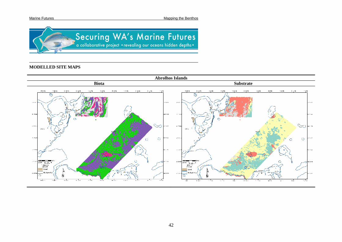
Abrolhos Islands: The southernmost study site has a vegetation and vegetation mixed with

sessile invertebrates. There is one site of hard corals approximately 2kms across. The northern

study site is predominately mixed vegetation and sessile invertebrates on soft sediments, with

small shallow reef areas dominated by some corals.

Jurien Bay: The majority of the area surveyed in Jurien Bay showed highly complex

topographic structures in the nearshore zone in the eastern study site, and along the ridge in

the southeastern section of the western study site. The northernmost study site has vegetation

in the shallow areas and soft sediment and rubble in the deeper areas off the ridge, which

increase in depth in the south-western quadrant.

Rottnest Island: Rottnest Island study area consists of high rugosity reefs generally

surrounding the island, while the deeper area to the west consisted of deep reefs in the eastern

portion with extensive sand beds to the west.

Cape Naturaliste west coast: Reefs (15 sq. km) are located primarily close to shore in the

north north-central parts of the mapping site, with isolated patches of lower lying reef further

from shore, and a large patch predicted at the outer limit of the southern part of the site.

Sediment (137 sq. km) covers the majority of the area, and reef outcrops are ringed by areas

of mixed sediment and reef (14 sq. km). Macroalgae was mapped mainly on exposed reef,

and covered a large portion of the site (34 sq. km vegetation), while sessile invertebrates

covered 8 sq. km, and a mix of vegetation and sessile invertebrates accounted for 36 sq km,

largely in the southern most part of the site.


35

Cape Naturaliste: Geographe Bay: The majority of the area surveyed in Geographe Bay has

soft substrate (86 sq. km); reef outcrops in the east, along a narrow ridge running east-west

(Four Mile Reef), patchily distributed in the north-north east and west, covering a total of 0.1

sq. km. More commonly classified than reef was a mixture of reef and sediment cover (5 sq.

km), which is widely distributed around the periphery of reef outcrops. The majority of the

area was vegetated (75 sq km) predominantly with seagrass (Amphibolis spp., Posidonia spp.)

near shore, and increasing contributions from macroalgae with increasing water depth.

Sessile invertebrates were mapped in areas with reef and mixed reef and sediment substrate (3

sq km). The lack of distinct topographic and potential ecologic gradients and ubiquity of

vegetation cover reduced the accuracy of the predictive modelling techniques used to map the

area.

Broke Inlet: The majority of Broke Inlet classified as sand. Sessile invertebrates were the

most common biotic coverage, while the second most common was algae. High medium and

low profile reef is found close to shore in the shallowest areas along with algae. High profile

reef is also found in the central southern section of the study site. Some areas of the site have

no substrate predicted, as none were modelled with acceptable confidence. Many of the same

areas not modelled for substrate, also were not modelled for biota, probably due to poor

sampling at the greater depths. At the reef-sand interface, a mixture of algae and sessile

invertebrates is predicted. Rhodoliths are predicted in approximately 40m depth in the north-

central section of the study site.

Albany (Mt Gardner):

The Mount Gardner site shows strong zonation related to depth and exposure to wave energy.

Shallow sheltered are dominated by seagrass, with increasing explore and depth this gives

way to mixed macroalgae, kelp and invertebrates. A small island situated in the western

central section of the site is dominated by kelp and the deeper water areas provide habitat for

sessile invertebrate communities.

Point Anne:

The Point Anne site shows pronounced depth zonation in biotic groups from shallow seagrass

areas grading into mixed macroalgae and sessile invertebrates. Extensive rhodolith beds are

found between 35 and 50 meters depth and finally deeper water sessile invertebrate

communities proliferate beyond 50 meters.


36

East Middle Island:

Distribution of biotic groups over the middle islands site reflects a combination of depth and

geomorphic features. Ridges which are relic coastlines provide substrate for seagrass in the

shallowest areas and macroalgae and sessile invertebrates beyond 15-20 meters. The Northern

eastern area of the site contains large areas of mixed vegetation and sessile invertebrates

below 50 meters. Similar areas in the southern portion of the site also have spares areas of

rhodolith presence. However the largest rhodoliths beds at this site are in the shallow Sothern

section of the site around 20 meters depth.

5.1 MAP APPLICATIONS AND INTERPRETATION The marine benthic mapping approach is based on statistical modelling and spatial prediction

to provide a more objective, quantitative alternative to traditional manually delineated marine

habitat maps. Individual benthic class models have proven effective for extending information

derived from towed-video footage over broader areas based on correlations with derivatives

of the bathymetry.

Video observations: The database of tow video observations assembled for modelling also

supplies a useful tally of the video footage content for use in other projects. For example, it

provides an index of georeferenced site descriptions, detailed information on classes not

included in the maps and other information such as good video footage. It will be useful for

planning monitoring and sample collection, if a particular benthos or substrate is required.

Models: Classification and regression tree (CART) models supply a robust and readily

interpretable framework for assessing the relative importance of environmental drivers over

broad spatial scales. In addition, the individual class model accuracy information (AUC,

misclassification rate, etc.) assists in understanding which maps are contributing the most

error, and can help guide how the maps are combined for multi-class mapping. Knowledge

gained from the modelling process can be used, in combination with sound biological and

ecological information, to better understand the causes and predictability of landscape scale

distribution patterns.

Presence/Absence maps: The maps of class presence and absence can be used for targeting

specific classes in the field for monitoring and/or assessment (e.g., find all locations where

macroalgae is present on reefs), or for locating class overlap by combining multiple maps.


37

Probability maps: Maps of probability of class presence are useful for targeting future

surveys, especially when individual classes are being considered. Additionally, areas with

probability values close to the cut off for presence/absence may be targeted in future surveys

to improve presence/absence predictions. In the final maps, areas which were not predicted as

present by any of the individual class models were left as undetermined.

It is not recommended that users combine probability maps for GIS-style numeric or

standardised binary overlay. Probability values produced by different models cannot be

interpreted in the same way. For example, in models for reef and algae, a probability of 0.35

could mean likely presence for reef and likely absence for algae. The binary presence/absence

maps always should be used for this purpose.

The field sites in this study include a wide range of coastal conditions, which means that

across the area, any particular type of biota may be responding to different ecological drivers

and thus show varying degrees of predictability. It is important to remember that bathymetry-

derived datasets are indirect drivers; they are not true physical drivers (e.g., light attenuation)

which are known to influence the distribution of biota. Thus, they are not necessarily directly

comparable for ecological interpretation across broad areas. While some of the biotic classes

mapped at higher taxonomic or hierarchical levels are the same at all mapped sites (e.g.,

Mixed brown algae), it is likely that many of the species comprising those classes differ from

site to site. This can also contribute to the selection of different dominant drivers through the

modelling process.

5.2 OUTCOME ISSUES AND SUGGESTIONS The benthic modelling and mapping component of Marine Futures is supplying some of the

first full coverage maps of the substrate and benthic sessile biota across several bioregions in

Western Australia; however, as with all research there remains room for improvement and

there are several issues to keep in mind while working with the final maps. The accuracy of

the final maps in how well they represent the present day benthos is directly linked to the

spatial layout and sub-sampling of the video footage.

There are several general issues in using video transects for statistical modelling that

influence model and map accuracy. One is that the changing quality of the video along

transect leads to inconsistent observations of detailed characteristics (e.g. presence of filter

feeders – only identifiable when the camera is very close to the seafloor), which leads to false

absences being used in the modelling process. The point location maps provide information


38

about where these features are most likely to be found based on the data available, but the

maps generally underestimate the true extent of distributions. The ratio of the number of

presences to absences for a single class has a significant impact on model development and

ultimately on map accuracy. For important but less abundant classes (e.g. invasive species),

gathering additional data with tow video or other collection methods may improve the

models. Using validation data from the same video transects used for modelling means the

data are not wholly independent. This can inflate the correct classification rates for the

models, giving an unrealistic impression of high mapping accuracy. In future work this can

be addressed by collecting a second, independent dataset for validation. Other issues related

to using transect-based sampling, such as orthogonal tow lines and excessive spatial

autocorrelation, may also impact models and their outputs, and require further investigation.

The accuracies reported refer to overall model accuracy. It should be noted that spatial

variability in the model fit may lead to extreme map errors in some areas. Due to the copious

amount of video collected for mapping, seven people participated in video analysis to ensure

completion in a timely fashion. However, integrating analyses by multiple interpreters also

led to some inconsistencies in identification of benthic classes, which were carried through

into the models.

While the presence/absence and combined maps provided the essential full coverage

information on general benthos features, other types of information would also be useful for

management, such as density of benthic vegetation and organisms. Unfortunately, the

changing size of the field of view in the towed video surveys meant that each video frame

shows a different (unmeasured) area, and prevents meaningful comparisons of density.

Further investigation is needed before recommendations can be made for improving this

aspect of the survey.

The backscatter data was found to be a strong predictor for some variables, but the processed

imagery contained a number of artefacts or errors in the data detectable as unrealistic linear

features. When the dataset was used to spatially extend the model over the full study area,

these artefacts are transferred to the final maps, and appear as striping.

6. CONCLUSION

The marine benthos maps and models provide extensive information on basic seafloor

physical properties and biology. Basic maps of substrate composition (reef, sediment) and


39

biota (vegetation, sessile invertebrates) presence and extent were produced to allow for state-

wide comparisons. For each site, all identified benthos classes with sufficient numbers of

observations for statistical modelling were mapped, showing the extent and patterns of

distribution for subclasses of sediment texture and relief, reef structures, vegetation types, and

different classes of sessile invertebrates. The layout of video transects, complexity of the

benthos, and clarity of the imagery influenced the accuracy and completeness of the video

observations. The models and maps reflect only what could be discerned from the video

footage; in areas where turbidity, distance from the bottom, or camera angle reduced

visibility, the recorded observations are likely not wholly accurate, but as the only available

information, were used for modelling and mapping. The models were robust, which is directly

related to the strong ecological gradients responding to spatially distinct environmental

driving variables, hypothesised to be wave exposure and light attenuation. Areas with weaker

biophysical gradients, eg. most of Geographe Bay, will always be modelled less successfully,

owing to the likely mismatch between the real processes controlling benthic patterns and the

independent variables possible to include for modelling. The biodiversity sampling campaign

will provide independent field validation of these habitat maps.


40

ACKNOWLEDGEMENTS

Video analysis by Ben Piek, Simon Grove, Christy Kirstner, Zarin Salter, Barbara Muhling,

Nisse Goldberg, Maya Salles-Taing, Janet Oswald, and Mike Byers. (UWA and WA

Fisheries). GIS support by Asha McNeill and Bryony Retter.

Hydroacoustic data collection and processing: Fugro Pty. Ltd., Perth, WA

The entire MF team, including Heather Taylor, Gary Kendrick, Jessica Meuuwig, and Euan

Harvey of UWA.


41

REFERENCES

Breiman L, Friedman JH, Olshen RA, Stone CG (1984) Classification and Regression Trees, Vol. Wadsworth International Group, Belmont, California, USA

Cochrane GR, Lafferty KD (2002) Use of acoustic classification of sidescan sonar

data for mapping benthic habitat in the Northern Channel Islands, California. Continental Shelf Research 22:683-690

De'ath G, Fabricius KE (2000) Classification and regression trees: A powerful yet

simple technique for ecological data analysis. Ecology 81:3178 Hosmer DW, Lemeshow S (2000) Applied logistic regression, Vol. Wiley, New York Jenness, J (2002) Surface Areas and Ratios from Elevation Grid (surfgrds.avx)

Extension for ArcView 3.x v. 1.2. Jenness Enterprises. Available at http://www.jennessent.com/arcfiew/surface_areas.htm.

Laffan, S (2003) Conversion of Splus/R decision tree into ArcInfo grid format. Arc

Macro Language

Liu C, Berry PM, Dawson TP, Pearson RG (2005) Selecting thresholds of occurrence in the prediction of species distributions. Ecography 28:385-393

Shokr ME (1991) Evaluation of second-order texture parameters for sea ice

classification from radar images. Journal of Geophysical Research 96:10625-10640 Schröder B, Richter O (1999) Are habitat models transferable in space and time? Z.

Okologie u Naturschutz 8:195-205


42

MODELLED SITE MAPS

Abrolhos Islands Biota Substrate


43


44

Jurien Bay

Biota Substrate


45

Rottnest Island

Biota Substrate


46

Geographe Bay

Biota Substrate


47

Cape Naturaliste

Biota Substrate


48

Broke Inlet

Biota Substrate


49

Mount Gardner

Biota Substrate


50

Point Anne

Biota Substrate


51

Middle Island

Biota Substrate

AW Marine Futures: BENTHIC MODELLING AND MAPPING...

Documents

Transcript of AW Marine Futures: BENTHIC MODELLING AND MAPPING...