Average Variance, Average Correlation and Currency Returns∗

Gino Cenedese

Bank of England

Lucio Sarno

Cass Business School and CEPR

Ilias Tsiakas

University of Guelph

First version: August 2011 - Revised: May 2012

Abstract

This paper provides an empirical investigation of the time-series predictive ability ofaverage variance and average correlation on the return to carry trades. Using quantileregressions, we find that higher average variance is significantly related to large futurecarry trade losses, whereas lower average correlation is significantly related to large gains.This is consistent with the carry trade unwinding in times of high volatility and the goodperformance of the carry trade when asset correlations are low. Finally, a new versionof the carry trade that conditions on average variance and average correlation generatesconsiderable performance gains net of transaction costs.

Keywords: Exchange Rates; Carry Trade; Average Variance; Average Correlation;

Quantile Regression.

JEL Classification: F31; G15; G17.

∗Acknowledgements: The authors are indebted for constructive comments to Bernard Dumas (editor),two anonymous referees, Pasquale Della Corte, Walter Distaso, Miguel Ferreira, Peter Gruber, Alex Maynard,Lukas Menkhoff, Francesco Nucci, Angelo Ranaldo, Pedro Santa-Clara, Maik Schmeling, Adrien Verdelhan,Paolo Volpin and Filip Zikes as well as to participants at the 2011 European Conference of the FinancialManagement Association, the 2011 ECB-Bank of Italy Workshop on Financial Determinants of ExchangeRates, the 2011 Rimini Centre Workshop in International Financial Economics, the 2010 INFINITI Conferenceon International Finance at Trinity College Dublin, the 2010 Transatlantic Doctoral Conference at LondonBusiness School, and the 2010 Spring Doctoral Conference at the University of Cambridge; as well as seminarparticipants at Goldman Sachs, Carleton University, Leibniz University Hannover and McMaster University.The views expressed in this paper are those of the authors, and not necessarily those of the Bank of England.Corresponding author: Lucio Sarno, Faculty of Finance, Cass Business School, 106 Bunhill Row, LondonEC1Y 8TZ, UK. Tel: +44 (0)20 7040 8772. Email: lucio.sarno@city.ac.uk. Other authors’ contact details:Gino Cenedese, email: gino.cenedese@bankofengland.co.uk. Ilias Tsiakas, email: itsiakas@uoguelph.ca.

1 Introduction

The carry trade is a popular currency trading strategy that invests in high-interest currencies

by borrowing in low-interest currencies. This strategy is designed to exploit deviations from

uncovered interest parity (UIP). If UIP holds, the interest rate differential is on average offset

by a commensurate depreciation of the investment currency and the expected carry trade

return is zero. There is extensive empirical evidence dating back to Bilson (1981) and Fama

(1984) that UIP is empirically rejected. In practice, it is often the case that high-interest

rate currencies appreciate rather than depreciate.1 As a result, over the last 35 years, the

carry trade has delivered sizeable excess returns and a Sharpe ratio more than twice that of

the US stock market (e.g., Burnside, Eichenbaum, Kleshchelski and Rebelo, 2011). It is no

surprise, therefore, that the carry trade has attracted enormous attention among academics

and practitioners.

An emerging literature argues that the high average return to the carry trade is no free

lunch in the sense that high carry trade payoffs compensate investors for bearing risk. The

risk measures used in this literature are specific to the foreign exchange (FX) market as tra-

ditional risk factors used to price stock returns fail to explain the returns to the carry trade

(e.g., Burnside, 2012). In a cross-sectional study, Menkhoff, Sarno, Schmeling and Schrimpf

(2012a) find that the large average carry trade payoffs are compensation for exposure to global

FX volatility risk. In times of high unexpected volatility, high-interest currencies deliver low

returns, whereas low-interest currencies perform well. This suggests that investors should

unwind their carry trade positions when volatility risk increases. Mueller, Stathopoulos and

Vedolin (2012) show that FX excess returns also carry a negative price of correlation risk,

where the latter is captured by the difference between average implied and average realized

correlation. Christiansen, Ranaldo and Soderlind (2011) further show that the risk exposure

of carry trade returns to stock and bond markets depends on the level of FX volatility. Lustig,

Roussanov and Verdelhan (2011) identify a slope factor in the cross section of FX portfolios

based on the excess return to the carry trade itself constructed in similar fashion to the Fama

1 The empirical rejection of UIP leads to the well-known forward bias, which is the tendency of the forwardexchange rate to be a biased predictor of the future spot exchange rate (e.g., Engel, 1996).

1

and French (1993) “high-minus-low” factor. Furthermore, Burnside, Eichenbaum, Kleshchel-

ski and Rebelo (2011) test whether the high carry trade payoffs reflect a peso problem, which

is a low probability of large negative payoffs. Although they do not find evidence of peso

events in their sample, they argue that investors still attach great importance to these events

and require compensation for them. Finally, Brunnermeier, Nagel, and Pedersen (2009) sug-

gest that carry trades are subject to crash risk that is exacerbated by the sudden unwinding

of carry trade positions when speculators face funding liquidity constraints.2

This paper investigates the intertemporal tradeoff between FX risk and the return to the

carry trade. We contribute to the recent literature cited above by focusing on four distinct

objectives. First, we set up a predictive framework, which differentiates this study from the

majority of the recent literature that is primarily concerned with the cross-sectional pricing of

FX portfolios. We are particularly interested in examining whether current market volatility

can predict the future carry trade return. Second, we evaluate the predictive ability of FX risk

on the full distribution of carry trade returns using quantile regressions, which are particularly

suitable for this purpose. In other words, we relate changes in FX risk to the large future

losses or gains of the carry trade located in the left or right tail of the return distribution

respectively. Predicting the full return distribution is useful for the portfolio choice of investors

(e.g., Cenesizoglu and Timmermann, 2010), and can also shed light on whether we can predict

currency crashes (e.g., Farhi et al., 2009; Jurek, 2009). Third, we define a set of FX risk

measures that capture well the movements in aggregate FX volatility and correlation. These

measures have recently been studied in the equities literature but are new to FX. Finally,

we assess the economic gains of our analysis by designing a new version of the carry trade

strategy that conditions on these FX risk measures.

The empirical analysis is organized as follows. The first step is to form a carry trade

portfolio that is rebalanced monthly using up to 33 US dollar nominal exchange rates. Our

initial measure of FX risk is the market variance defined as the variance of the returns to the

FX market portfolio. We then take a step further by decomposing the market variance in two

components: the cross-sectional average variance and the cross-sectional average correlation,

2 Similar arguments based on crash risk and disaster premia are put forth by Farhi, Fraiberger, Gabaix,Ranciere and Verdelhan (2009) and Jurek (2009).

2

implementing the methodology applied by Pollet and Wilson (2010) to predict equity returns.

Next, using quantile regressions, we assess the predictive ability of average variance and av-

erage correlation on the full distribution of carry trade returns. Quantile regressions provide

a natural way of assessing the effect of higher risk on different parts (quantiles) of the carry

return distribution. Finally, we design an augmented carry trade strategy that conditions on

average variance and average correlation. This new version of the carry trade is implemented

out of sample and accounts for transaction costs.

We find that the product of average variance and average correlation captures more than

90% of the time-variation in the FX market variance, suggesting that this decomposition works

very well empirically. More importantly, the decomposition of market variance into average

variance and average correlation is found to be crucial for understanding empirically the risk-

return tradeoff in FX. Average variance has a significant negative effect on the left tail of

future carry trade returns, whereas average correlation has a significant negative effect on the

right tail. This implies that: (i) higher average variance is significantly related to large losses

in the future returns to the carry trade, potentially leading investors to unwind their carry

trade positions, and (ii) lower average correlation is significantly related to large future carry

trade returns by enhancing the gains of diversification. Market variance is a weaker predictor

than average variance and average correlation because, by aggregating information about the

latter two risk measures into one risk measure, market variance becomes less informative than

using average variance and average correlation separately. Finally, the augmented carry trade

strategy that conditions on average variance and average correlation performs considerably

better than the standard carry trade, even accounting for transaction costs. Taken together,

these results imply the existence of a meaningful predictive relation between average variance,

average correlation and carry trade returns: average variance and average correlation predict

currency returns when it matters most, namely when returns are large (negative or positive),

whereas the relation may be non-existent in normal times.

Furthermore, we show that the predictive ability of average variance and average corre-

lation is robust to the inclusion of additional predictive variables such as the interest rate

differential and the lagged carry return. It is also robust to changing the numeraire from the

3

US dollar to a composite numeraire that is based on the US dollar, the euro, the UK pound

and the Japanese yen. We further demonstrate that implied volatility indices, such as the

VIX for the equities market and the VXY for the FX market, are not significant predictors of

future carry returns, and hence cannot replicate the predictive information in average variance

and average correlation.

The remainder of the paper is organized as follows. In the next section we provide a brief

overview of the literature on the intertemporal tradeoff between risk and return, and motivate

the empirical predictions we examine in this paper. In Section 3 we describe the FX data

set and define the measures for risk and return on the carry trade. Section 4 presents the

predictive quantile regressions and discusses estimation issues. In Section 5, we report the

empirical results, followed by robustness checks and further analysis in Section 6. Section 7

discusses the augmented carry trade strategies and, finally, Section 8 concludes.

2 The Intertemporal Tradeoff between FX Risk and Re-

turn: A Brief Review and Testable Implications

Since the Intertemporal Capital Asset Pricing Model (ICAPM) of Merton (1973, 1980), a class

of asset pricing models has developed which suggests an intertemporal tradeoff between risk

and return. These models hold for any risky asset in any market and hence can be applied not

only to equities but also to the FX market. For the carry trade, the intertemporal risk-return

tradeoff may be expressed as follows:

rC,t+1 = µ+ κσ2t + εt+1 (1)

σ2t = ϕ0 + ϕ1AVt + ϕ2ACt (2)

where rC,t+1 is the return to the carry trade portfolio from time t to t+1; σ2t is the conditional

variance of the returns to the FX market portfolio at time t, termed the FX market variance;

AVt is the equally weighted cross-sectional average of the variances of all exchange rate excess

returns at time t; ACt is the equally weighted cross-sectional average of the pairwise corre-

4

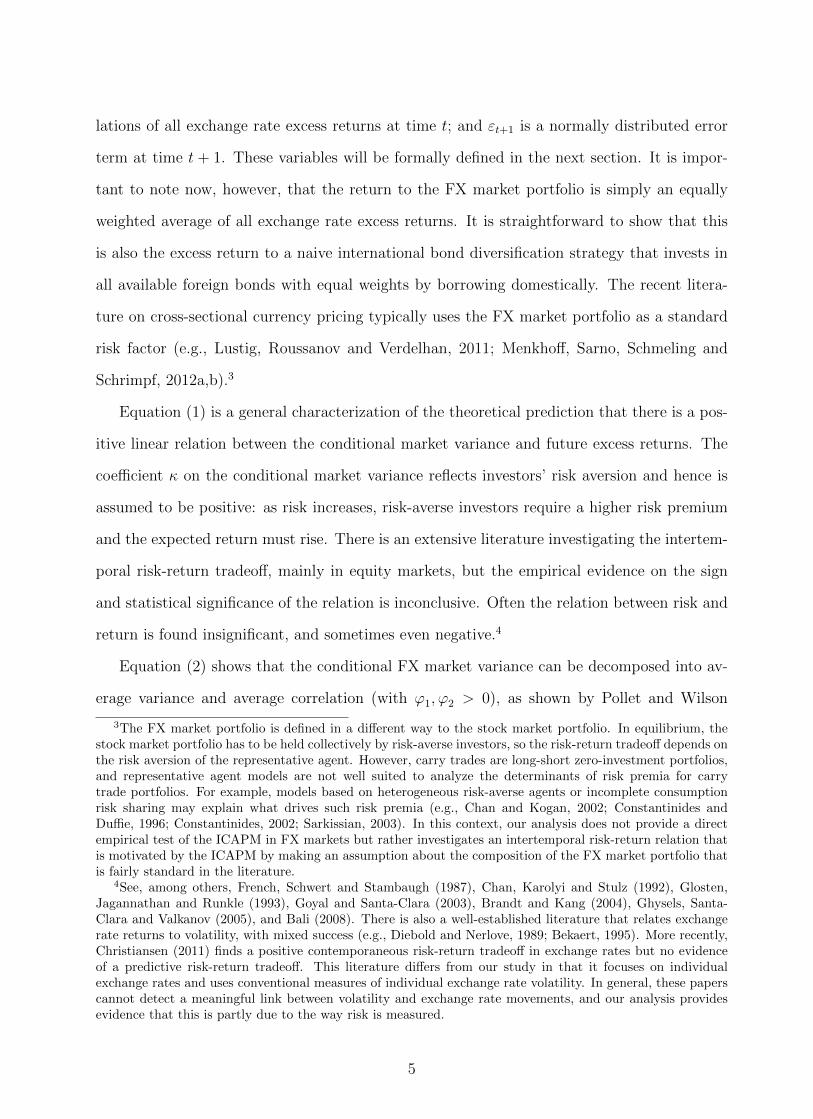
lations of all exchange rate excess returns at time t; and εt+1 is a normally distributed error

term at time t + 1. These variables will be formally defined in the next section. It is impor-

tant to note now, however, that the return to the FX market portfolio is simply an equally

weighted average of all exchange rate excess returns. It is straightforward to show that this

is also the excess return to a naive international bond diversification strategy that invests in

all available foreign bonds with equal weights by borrowing domestically. The recent litera-

ture on cross-sectional currency pricing typically uses the FX market portfolio as a standard

risk factor (e.g., Lustig, Roussanov and Verdelhan, 2011; Menkhoff, Sarno, Schmeling and

Schrimpf, 2012a,b).3

Equation (1) is a general characterization of the theoretical prediction that there is a pos-

itive linear relation between the conditional market variance and future excess returns. The

coefficient κ on the conditional market variance reflects investors’ risk aversion and hence is

assumed to be positive: as risk increases, risk-averse investors require a higher risk premium

and the expected return must rise. There is an extensive literature investigating the intertem-

poral risk-return tradeoff, mainly in equity markets, but the empirical evidence on the sign

and statistical significance of the relation is inconclusive. Often the relation between risk and

return is found insignificant, and sometimes even negative.4

Equation (2) shows that the conditional FX market variance can be decomposed into av-

erage variance and average correlation (with ϕ1, ϕ2 > 0), as shown by Pollet and Wilson

3The FX market portfolio is defined in a different way to the stock market portfolio. In equilibrium, thestock market portfolio has to be held collectively by risk-averse investors, so the risk-return tradeoff depends onthe risk aversion of the representative agent. However, carry trades are long-short zero-investment portfolios,and representative agent models are not well suited to analyze the determinants of risk premia for carrytrade portfolios. For example, models based on heterogeneous risk-averse agents or incomplete consumptionrisk sharing may explain what drives such risk premia (e.g., Chan and Kogan, 2002; Constantinides andDuffie, 1996; Constantinides, 2002; Sarkissian, 2003). In this context, our analysis does not provide a directempirical test of the ICAPM in FX markets but rather investigates an intertemporal risk-return relation thatis motivated by the ICAPM by making an assumption about the composition of the FX market portfolio thatis fairly standard in the literature.

4See, among others, French, Schwert and Stambaugh (1987), Chan, Karolyi and Stulz (1992), Glosten,Jagannathan and Runkle (1993), Goyal and Santa-Clara (2003), Brandt and Kang (2004), Ghysels, Santa-Clara and Valkanov (2005), and Bali (2008). There is also a well-established literature that relates exchangerate returns to volatility, with mixed success (e.g., Diebold and Nerlove, 1989; Bekaert, 1995). More recently,Christiansen (2011) finds a positive contemporaneous risk-return tradeoff in exchange rates but no evidenceof a predictive risk-return tradeoff. This literature differs from our study in that it focuses on individualexchange rates and uses conventional measures of individual exchange rate volatility. In general, these paperscannot detect a meaningful link between volatility and exchange rate movements, and our analysis providesevidence that this is partly due to the way risk is measured.

5

(2010) for equity returns. This decomposition is an aspect of our analysis that is critical for

distinguishing the effect of systematic and idiosyncratic risk on future carry trade returns

as well as for delivering robust and statistically significant results in predicting future carry

trade returns. For example, Goyal and Santa-Clara (2003) show that although the equally

weighted market variance only reflects systematic risk, average variance captures both sys-

tematic and idiosyncratic risk and is a more powerful predictor of future equity returns than

market variance. This implies that idiosyncratic risk matters for equity returns and our anal-

ysis investigates whether this is also the case for FX excess returns.5

Furthermore, standard finance theory suggests that lower asset correlations generally lead

to improved diversification and better portfolio performance. This is also the case for carry

trade strategies, as shown by Burnside, Eichenbaum and Rebelo (2008), who demonstrate

that the gains of diversifying the carry trade across many currencies are large, raising the

Sharpe ratio by over 50 percent. In a cross-sectional study, Mueller, Stathopoulos and Vedolin

(2012) demonstrate that currency portfolios with low or negative exposure to correlation risk

perform well. More to the point, Pollet and Wilson (2010) show that the average correlation

of stocks is positively related to future stock returns. In the context of the ICAPM, they argue

that since the return on aggregate wealth is not directly observable (Roll, 1977), changes in

aggregate risk may reveal themselves through changes in the correlation between observable

stock returns. Hence an increase in aggregate risk can be related to higher average correlation

and higher future stock returns. In light of the above, the first testable hypothesis of the

empirical analysis is as follows:

H1: FX risk measures based on average variance and average correlation are more powerful

predictors than market variance for future FX excess returns.

The intertemporal risk-return model of Equations (1)–(2) can be applied to the full con-

ditional distribution of returns. The τ -th conditional quantile function for rC,t+1 implied by

5There are a number of theoretical models and economic arguments that justify why a market-wide mea-sure of idiosyncratic risk may matter for returns. For example, variants of the CAPM where investors holdundiversified portfolios for either rational (tax or transactions costs) or irrational reasons predict an intertem-poral relation between returns and idiosyncratic risk (see Goyal and Santa-Clara, 2003, for a discussion of thisliterature). This relation also obtains in a cross-sectional context in models with incomplete risk sharing (e.g.,Sarkissian, 2003).

6

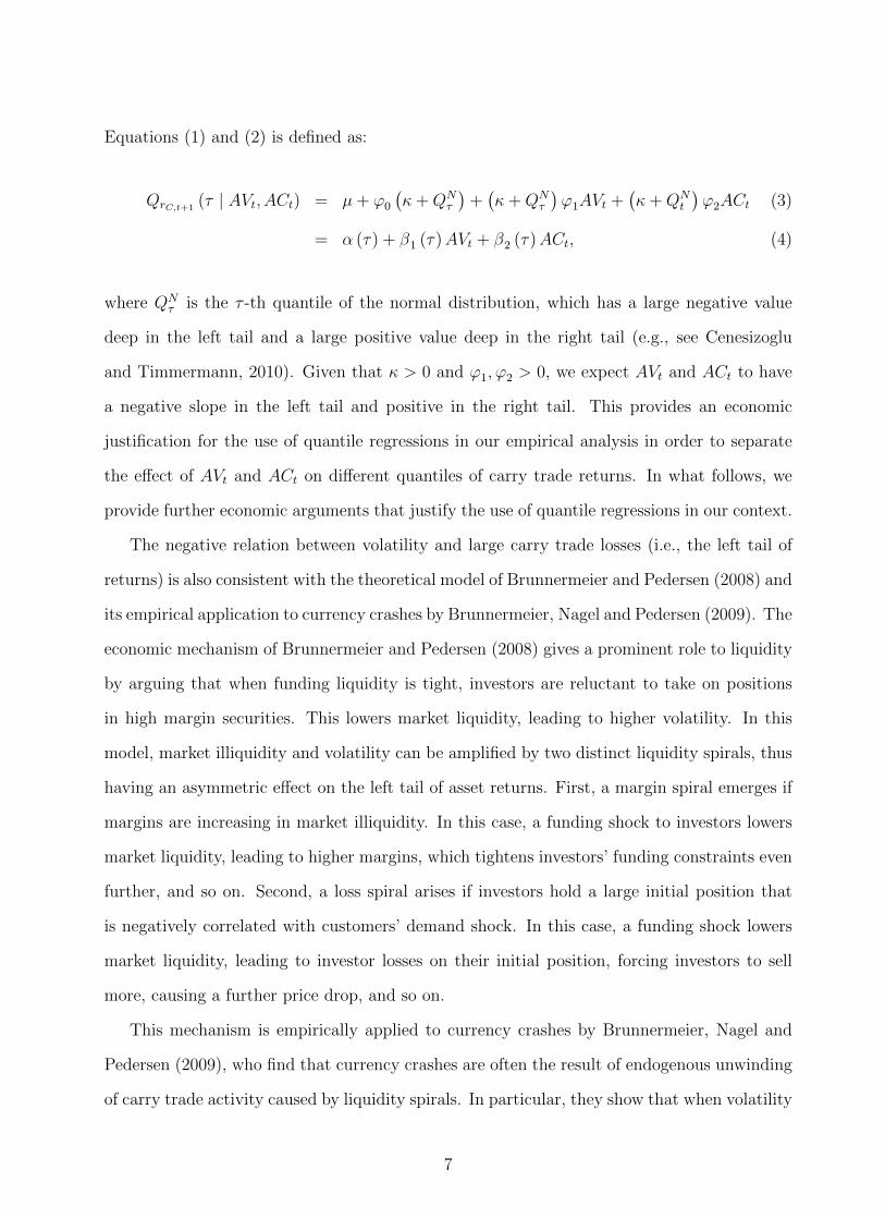
Equations (1) and (2) is defined as:

QrC,t+1(τ | AVt, ACt) = µ+ ϕ0

(κ+QN

τ

)+(κ+QN

τ

)ϕ1AVt +

(κ+QN

t

)ϕ2ACt (3)

= α (τ) + β1 (τ)AVt + β2 (τ)ACt, (4)

where QNτ is the τ -th quantile of the normal distribution, which has a large negative value

deep in the left tail and a large positive value deep in the right tail (e.g., see Cenesizoglu

and Timmermann, 2010). Given that κ > 0 and ϕ1, ϕ2 > 0, we expect AVt and ACt to have

a negative slope in the left tail and positive in the right tail. This provides an economic

justification for the use of quantile regressions in our empirical analysis in order to separate

the effect of AVt and ACt on different quantiles of carry trade returns. In what follows, we

provide further economic arguments that justify the use of quantile regressions in our context.

The negative relation between volatility and large carry trade losses (i.e., the left tail of

returns) is also consistent with the theoretical model of Brunnermeier and Pedersen (2008) and

its empirical application to currency crashes by Brunnermeier, Nagel and Pedersen (2009). The

economic mechanism of Brunnermeier and Pedersen (2008) gives a prominent role to liquidity

by arguing that when funding liquidity is tight, investors are reluctant to take on positions

in high margin securities. This lowers market liquidity, leading to higher volatility. In this

model, market illiquidity and volatility can be amplified by two distinct liquidity spirals, thus

having an asymmetric effect on the left tail of asset returns. First, a margin spiral emerges if

margins are increasing in market illiquidity. In this case, a funding shock to investors lowers

market liquidity, leading to higher margins, which tightens investors’ funding constraints even

further, and so on. Second, a loss spiral arises if investors hold a large initial position that

is negatively correlated with customers’ demand shock. In this case, a funding shock lowers

market liquidity, leading to investor losses on their initial position, forcing investors to sell

more, causing a further price drop, and so on.

This mechanism is empirically applied to currency crashes by Brunnermeier, Nagel and

Pedersen (2009), who find that currency crashes are often the result of endogenous unwinding

of carry trade activity caused by liquidity spirals. In particular, they show that when volatility

7

increases, the carry trade tends to incur losses and the volume of currency trading tends to

decrease. More importantly, negative shocks have a much larger effect on returns than positive

shocks in the following sense. During high volatility, shocks that lead to losses are amplified

when investors hit funding constraints and unwind their positions, further depressing prices,

thus increasing the funding problems and volatility. Conversely, shocks that lead to gains are

not amplified. This asymmetric effect indicates that not only is volatility negatively related

to carry trade returns but high volatility has a much stronger effect on the left tail of carry

returns than in the right tail. This economic mechanism based on liquidity spirals relates

volatility to future carry trade losses and is consistent with Equations (3) and (4). Hence, the

second testable hypothesis of our empirical analysis is:

H2: The predictive power of average variance and average correlation varies across quan-

tiles of the distribution of FX excess returns, and is strongly negative in the lower quantiles.

2.1 Other Related Literature

This paper is also related to Bali and Yilmaz (2011), who estimate two types of predictive

regressions based on the ICAPM: first, of individual FX returns on individual variances, for

which they find a positive but statistically insignificant relation; and second, of individual

FX returns on the covariance between individual exchange rates and the FX market variance,

for which they find a positive and statistically significant relation. Our analysis, however,

substantially deviates from Bali and Yilmaz (2011) in a number of ways: (i) we focus on the

carry trade portfolio, not on individual exchange rates; (ii) we analyze a larger number of

currencies (33 versus 6 exchange rates) and a longer sample (34 years versus 7 years); (iii) we

decompose the market variance into average variance and average correlation; (iv) we assess

predictability across the full distribution of carry trade returns using quantile regressions; and

(v) we design a new carry trade strategy that conditions on average variance and average

correlation to assess the economic significance of our statistical findings.

The risk measures employed in our analysis have been the focus of recent intertemporal as

well as cross-sectional studies of the equity market. The intertemporal role of average variance

is examined by Goyal and Santa-Clara (2003), as discussed earlier, and also by Bali, Cakici,

8

Yan and Zhang (2005). These studies show that average variance reflects both systematic

and idiosyncratic risk and is significantly positively related to future equity returns. In the

cross section of equity returns, the negative price of risk associated with market variance is

examined by Ang, Hodrick, Xing and Zhang (2006, 2009). They find that stock portfolios with

high sensitivities to innovations in aggregate volatility have low average returns. Similarly,

Krishnan, Petkova and Ritchken (2009) find a negative price of risk for equity correlations.

Finally, Chen and Petkova (2011) examine the cross-sectional role of average variance and

average correlation. They find that for portfolios sorted by size and idiosyncratic volatility,

average variance has a negative price of risk, whereas average correlation is not priced.

3 Measures of Return and Risk for the Carry Trade

This section describes the FX data set and defines our measures for: (i) the excess return to

the carry trade for individual currencies, (ii) the excess return to the carry trade for a portfolio

of currencies, and (iii) three measures of risk: market variance, average variance, and average

correlation.

3.1 FX Data

We use a cross section of US dollar nominal spot and forward exchange rates by collecting

data on 33 currencies relative to the US dollar: Australia, Austria, Belgium, Canada, Czech

Republic, Denmark, Euro area, Finland, France, Germany, Greece, Hong Kong, Hungary,

India, Ireland, Italy, Japan, Mexico, Netherlands, New Zealand, Norway, Philippines, Poland,

Portugal, Saudi Arabia, Singapore, South Africa, South Korea, Spain, Sweden, Switzerland,

Taiwan and United Kingdom. The sample period runs from January 1976 to February 2009.

Note that the number of exchange rates for which there are available data varies over time;

at the beginning of the sample we have data for 15 exchange rates, whereas at the end we

have data for 22. The data are collected by WM/Reuters and Barclays and are available on

Thomson Financial Datastream. The exchange rates are listed in Table 1.

9

3.2 The Carry Trade for Individual Currencies

An investor can implement a carry trade strategy for either individual currencies or, more

commonly in the practice of currency management, a portfolio of currencies. The carry trade

strategy for individual currencies can be implemented in one of two equivalent ways. First, the

investor may buy a forward contract now for exchanging the domestic currency into foreign

currency in the future. She may then convert the proceeds of the forward contract into the

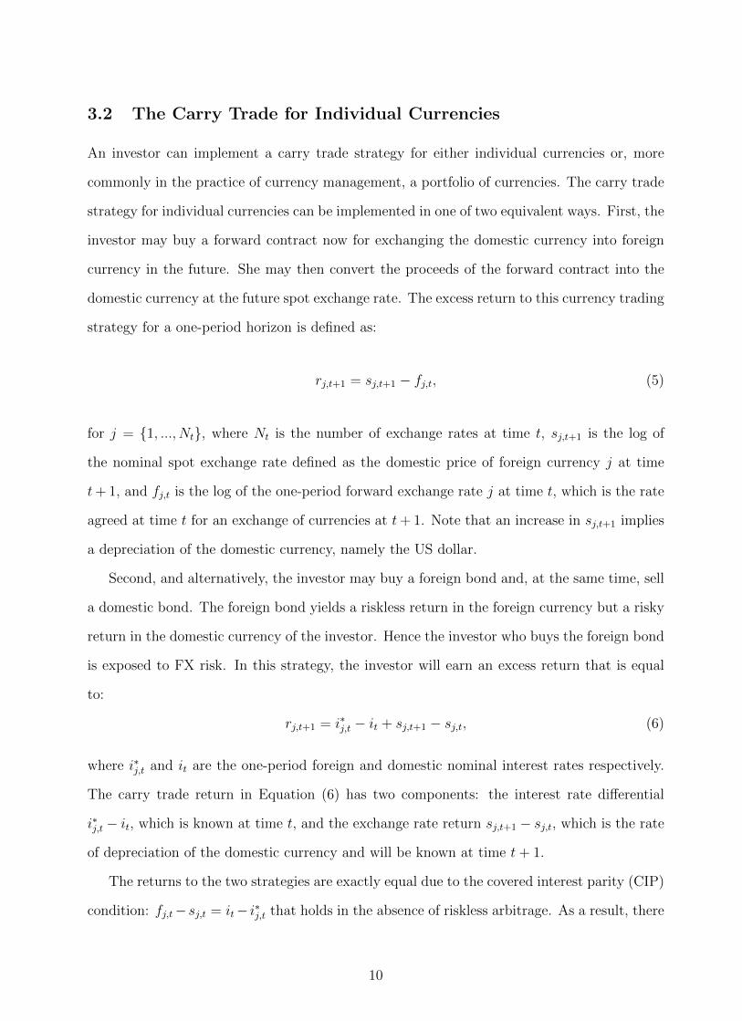
domestic currency at the future spot exchange rate. The excess return to this currency trading

strategy for a one-period horizon is defined as:

rj,t+1 = sj,t+1 − fj,t, (5)

for j = {1, ..., Nt}, where Nt is the number of exchange rates at time t, sj,t+1 is the log of

the nominal spot exchange rate defined as the domestic price of foreign currency j at time

t+ 1, and fj,t is the log of the one-period forward exchange rate j at time t, which is the rate

agreed at time t for an exchange of currencies at t+ 1. Note that an increase in sj,t+1 implies

a depreciation of the domestic currency, namely the US dollar.

Second, and alternatively, the investor may buy a foreign bond and, at the same time, sell

a domestic bond. The foreign bond yields a riskless return in the foreign currency but a risky

return in the domestic currency of the investor. Hence the investor who buys the foreign bond

is exposed to FX risk. In this strategy, the investor will earn an excess return that is equal

to:

rj,t+1 = i∗j,t − it + sj,t+1 − sj,t, (6)

where i∗j,t and it are the one-period foreign and domestic nominal interest rates respectively.

The carry trade return in Equation (6) has two components: the interest rate differential

i∗j,t − it, which is known at time t, and the exchange rate return sj,t+1 − sj,t, which is the rate

of depreciation of the domestic currency and will be known at time t+ 1.

The returns to the two strategies are exactly equal due to the covered interest parity (CIP)

condition: fj,t−sj,t = it− i∗j,t that holds in the absence of riskless arbitrage. As a result, there

10

is an equivalence between trading currencies through spot and forward contracts and trading

international bonds.6 The return rj,t+1 defined in Equations (5) and (6) is also known as the

FX excess return.

If UIP holds, then the excess return in Equations (5) and (6) will on average be equal

to zero, and hence the carry trade will not be profitable. In other words, under UIP, the

interest rate differential will on average be exactly offset by a commensurate depreciation of

the investment currency. However, as mentioned earlier, it is extensively documented that

UIP is empirically rejected so that high-interest rate currencies tend to appreciate rather

than depreciate (e.g., Bilson, 1981; Fama, 1984). The empirical rejection of UIP implies that

the carry trade for either individual currencies or portfolios of currencies tends to be highly

profitable (e.g., Della Corte, Sarno and Tsiakas, 2009; Burnside, Eichenbaum, Kleshchelski

and Rebelo, 2011).

3.3 The Carry Trade for a Portfolio of Currencies

There are many versions of the carry trade for a portfolio of currencies and, in this paper, we

implement one of the most popular. We form a portfolio by sorting at the beginning of each

month all currencies according to the value of the forward premium fj,t − sj,t. If CIP holds,

sorting currencies from low to high forward premium is equivalent to sorting from high to

low interest rate differential. We then divide the total number of currencies available in that

month in five portfolios (quintiles), as in Menkhoff, Sarno, Schmeling and Schrimpf (2012a).

Portfolio 1 is the portfolio with the highest interest rate currencies, whereas Portfolio 5 has the

lowest interest rate currencies. The monthly return to the carry trade portfolio is the excess

return of going long on Portfolio 1 and short on Portfolio 5. In other words, the carry trade

portfolio borrows in low-interest rate currencies and invests in high-interest rate currencies.

6There is ample empirical evidence that CIP holds in practice for the data frequency examined in thispaper. For recent evidence, see Akram, Rime and Sarno (2008). The only exception in our sample is theperiod following Lehman’s bankruptcy, when the CIP violation persisted for a few months (e.g., Mancini-Griffoli and Ranaldo, 2011).

11

3.4 FX Market Variance

Our first measure of risk is the FX market variance, which captures the aggregate variance in

FX. Note that this measure of market variance focuses exclusively on the FX market, and hence

it is not the same as the market variance used in equity studies (e.g., Pollet and Wilson, 2010).

Specifically, FX market variance is the variance of the return to the FX market portfolio. We

define the excess return to the FX market portfolio as the equally weighted average of the

excess returns of all exchange rates:7

rM,t+1 =1

Nt

Nt∑j=1

rj,t+1. (7)

This can be thought of as the excess return to a naive 1/Nt currency trading strategy, or

an international bond diversification strategy that buys Nt foreign bonds (i.e., all available

foreign bonds in the opportunity set of the investor at time t) by borrowing domestically.8

We estimate the monthly FX market variance (MV) using a realized measure based on

daily excess returns:

MVt+1 =Dt∑d=1

r2M,t+d/Dt+ 2

Dt∑d=2

rM,t+d/DtrM,t+(d−1)/Dt , (8)

where Dt is the number of trading days in month t, and typically Dt = 21. Following French,

Schwert and Stambaugh (1987), Goyal and Santa-Clara (2003), and Bali, Cakici, Yan and

Zhang (2005), among others, this measure of market variance accounts for the autocorrelation

in daily returns.9

7We use equal weights as it would be difficult to determine time-varying “value” weights on the basis ofmonthly turnover for each currency over our long sample range. Menkhoff, Sarno, Schmeling and Schrimpf(2012a) weigh the volatility contribution of different currencies by their share in international currency reservesin a given year and find no significant differences relative to equal weights.

8Note that the direction of trading does not affect the FX market variance. If instead the US investordecides to lend 1 US dollar by buying a domestic US bond and selling Nt foreign bonds with equal weights,the excess return to the portfolio would be r∗M,t+1 = −rM,t+1. However, the market variance would remain

unaffected: V(r∗M,t+1

)= V (−rM,t+1) = V (rM,t+1).

9This is similar to the heteroskedasticity and autocorrelation consistent (HAC) measure of Bandi and Perron(2008), which uses linearly decreasing Bartlett weights on the realized autocovariances. Our empirical resultsremain practically identical when using the HAC market variance, and hence we use the simpler specificationof Equation (8) in our analysis.

12

3.5 Average Variance and Average Correlation

Our second set of risk measures relies on the Pollet and Wilson (2010) decomposition of MV

into the product of two terms, the cross-sectional average variance (AV) and the cross-sectional

average correlation (AC), as follows:

MVt+1 = AVt+1 × ACt+1. (9)

The decomposition would be exact if all exchange rates had equal individual variances,

but is actually approximate given that exchange rates display unequal variances. Thus, the

validity of the decomposition is very much an empirical matter. Pollet and Wilson (2010) use

this decomposition for a large number of stocks and find that the approximation works very

well. As we show later, this approximation works remarkably well also for exchange rates.

We can assess the empirical validity of the decomposition by estimating the following

regression:

MVt+1 = α + β (AVt+1 × ACt+1) + ut+1, (10)

where E [ut+1 | AVt+1 × ACt+1] = 0. The coefficient β may not be equal to one because

exchange rates do not have the same individual variance and there may be measurement error

in MVt+1, AVt+1 and ACt+1. However, the R2 of this regression will give us a good indication

of how well the decomposition works empirically.

We estimate AV and AC as follows:

AVt+1 =1

Nt

Nt∑j=1

Vj,t+1, (11)

ACt+1 =1

Nt(Nt − 1)

Nt∑i=1

Nt∑j 6=i

Cij,t+1, (12)

where Vj,t+1 is the realized variance of the excess return to exchange rate j at time t + 1

computed as

Vj,t+1 =Dt∑d=1

r2j,t+d/Dt+ 2

Dt∑d=2

rj,t+d/Dtrj,t+(d−1)/Dt , (13)

13

and Cij,t+1 is the realized correlation between the excess returns of exchange rates i and j at

time t+ 1 computed as

Cij,t+1 =Vij,t+1√

Vi,t+1

√Vj,t+1

, (14)

Vij,t+1 =Dt∑d=1

ri,t+d/Dtrj,t+d/Dt + 2Dt∑d=2

ri,t+d/Dtrj,t+(d−1)/Dt . (15)

Note that we do not demean returns in calculating variances. This allows us to avoid esti-

mating mean returns and has very little impact on calculating variances (see, e.g., French,

Schwert and Stambaugh, 1987).10

3.6 Systematic and Idiosyncratic Risk

Define Vj,d as the variance of the excess return to exchange rate j on day d. In this section

only, for notational simplicity we suppress the monthly index t. Then, Vj,d is a measure of

total risk that contains both systematic and idiosyncratic components. Following Goyal and

Santa-Clara (2003), we can decompose these two parts of total risk as follows. Suppose that

the excess return rj,d is driven by a common factor µd and an idiosyncratic zero-mean shock

εj,d that is specific to exchange rate j. For simplicity, further assume that the factor loading

for each exchange rate is equal to one, the common and idiosyncratic factors are uncorrelated,

and ignore the serial correlation adjustment in Equation (13). Then, the data generating

process for daily returns is:

rj,d = µd + εj,d, (16)

and the return to the FX market portfolio for day d on a given month t is:

rM,d =1

Nt

Nt∑j=1

rj,d = µd +1

Nt

Nt∑j=1

εj,d, (17)

where the second term becomes negligible for large Nt.

10 For our main analysis, we compute monthly measures of MV, AV and AC using daily returns. In therobustness section, we show that these are highly correlated to monthly measures based on intraday returns.As intraday data are only available for a shorter sample and a much smaller cross section, we employ themonthly measures based on daily returns for our core analysis.

14

It is straightforward to show that on a given month t:

MV =Dt∑d=1

r2M,d =Dt∑d=1

µ2d +

2

Nt

µd

Nt∑j=1

εj,d +

(1

Nt

Nt∑j=1

εj,d

)2 , (18)

AV =Dt∑d=1

[1

Nt

Nt∑j=1

r2j,d

]=

Dt∑d=1

[µ2d +

2

Nt

µd

Nt∑j=1

εj,d +1

Nt

Nt∑j=1

ε2j,d

]. (19)

The first two terms of MV and AV are identical and capture the systematic component of

total risk as they depend on the common factor. The third term that depends exclusively on

the idiosyncratic component is different for MV and AV. For a large cross section of exchange

rates, this term is negligible for MV, and hence MV does not reflect any idiosyncratic risk.

For AV, however, the third term is not negligible and captures the idiosyncratic component

of total risk.

To get a better idea of the relative size of the systematic and idiosyncratic components,

consider the following example based on the descriptive statistics of Table 2. In annualized

terms, the expected monthly variances are:

E [MV ]× 103 = 5 =Systematic︸ ︷︷ ︸

5

+Idiosyncratic︸ ︷︷ ︸

0

, (20)

E [AV ]× 103 = 10 =Systematic︸ ︷︷ ︸

5

+Idiosyncratic︸ ︷︷ ︸

5

. (21)

Therefore, half of the risk captured by AV in FX is systematic and the other half is idiosyn-

cratic, whereas all of the risk reflected in MV is systematic.

Similarly, the standard deviations are:

STD [MV ]× 103 = 2, (22)

STD [AV ]× 103 = 3. (23)

As a result, the t-ratio of mean divided by standard deviation is 2.5 for MV and 3.3 for AV. In

other words, AV is measured more precisely than MV, which can possibly make AV a better

15

predictor of FX excess returns.

4 Predictive Regressions

Our empirical analysis begins with ordinary least squares (OLS) estimation of two predictive

regressions for a one-month ahead horizon. The first predictive regression provides a simple

way for assessing the intertemporal risk-return tradeoff in FX as follows:

rC,t+1 = α + βMVt + εt+1, (24)

where rC,t+1 is the return to the carry trade portfolio from time t to t + 1, and MVt is the

market variance from time t − 1 to t. This regression will capture whether, on average, the

carry trade has low or negative returns following times of high market variance.

The second predictive regression assesses the risk-return tradeoff implied by the decompo-

sition of market variance into average variance and average correlation:

rC,t+1 = α + β1AVt + β2ACt + εt+1, (25)

where AVt and ACt are the average variance and average correlation from time t − 1 to t.

For notational simplicity, we use the same symbol α for the constants in the two regressions.

The second regression separates the effect of AV and AC in order to determine whether the

decomposition provides a more precise signal for future carry returns.

The simple OLS regressions focus on the effect of the risk measures on the conditional mean

of future carry returns. We go further by also estimating two predictive quantile regressions,

which are designed to capture the conditional effect of either MV or AV and AC on the full

distribution of future carry returns. It is possible, for example, that average variance is a

poor predictor of the conditional mean return but predicts well one or both tails of the return

distribution. Using quantile regressions provides a natural way of assessing the effect of higher

risk on different parts of the distribution of future carry returns. It is also an effective way

of dealing with outliers. For example, the median is a quantile of particular importance that

16

allows for direct comparison to the OLS regression, which focuses on the conditional mean.

It is well known that outliers may have a larger effect on the mean of a distribution than the

median. Hence the quantile regressions can provide more robust results than OLS regressions

even for the middle of the distribution. In our analysis, we focus on deciles of the distribution

of future carry returns.

The first predictive quantile regression estimates:

QrC,t+1(τ |MVt) = α (τ) + β (τ)MVt, (26)

where QrC,t+1(τ | ·) is the τ -th quantile function of the one-month ahead carry trade returns

conditional on information available at time t.11

The second predictive quantile regression yields estimates of the τ -th conditional quantile

function:

QrC,t+1(τ | AVt, ACt) = α (τ) + β1 (τ)AVt + β2 (τ)ACt. (27)

The standard error of the quantile regression parameters is estimated using a moving block

bootstrap (MBB) that provides inference robust to heteroskedasticity and autocorrelation of

unknown form (Fitzenberger, 1997). Specifically, we employ a circular MBB of the residuals

as in Politis and Romano (1992). The optimal block size is selected using the automatic

procedure of Politis and White (2004) and Patton, Politis and White (2009). The bootstrap

algorithm is detailed in the Appendix.

5 Empirical Results

5.1 Descriptive Statistics

Table 2 reports descriptive statistics on the following variables: (i) the return to the carry trade

11We obtain estimates of the quantile regression coefficients {α (τ) , β (τ)} by solving the minimizationproblem min

α,β

∑[ρτ (rC,t+1 − α (τ)− β (τ)MVt)], using the asymmetric loss function ρτ (u) = u (τ − I (u < 0)).

We formulate the optimization problem as a linear program and solve it by implementing the interior pointmethod of Portnoy and Koenker (1997). See also Koenker (2005, Chapter 6).

17

portfolio; (ii) the return to the exchange rate and interest rate components of the carry trade

return; (iii) the excess return to the FX market portfolio; (iv) the FX market variance (MV);

and (v) the FX average variance (AV) and average correlation (AC). Assuming no transaction

costs, the carry trade delivers an annualized mean return of 8.6%, a standard deviation of

7.8% and a Sharpe ratio of 1.092. The carry trade return is primarily due to the interest rate

differential across countries, which delivers an average return of 13.7%. The exchange rate

depreciation component has a return of −5.1%, indicating that on average exchange rates only

partially offset the interest rate differential. The carry trade return displays negative skewness

of −0.967 and kurtosis of 6.043. These statistics confirm the good historical performance of the

carry trade and are consistent with the literature (e.g., Burnside, Eichenbaum, Kleshchelski

and Rebelo, 2011). Finally, the average market return is low at 1.0% per year, and its standard

deviation is the same as that of the carry trade return at 7.8%.

Turning to the risk measures, the mean of MV is 0.005. The mean of AV is double that of

MV at 0.010, and the mean of AC is 0.471. MV and AV exhibit high positive skewness and

massive kurtosis. The time variation of AV and AC together with the cumulative carry trade

return are displayed in Figure 1.

Panel B of Table 2 shows the cross-correlations. The correlation between the excess returns

on the carry and the market portfolio is 9.1%. The three risk measures are positively correlated

with each other but negatively correlated with the carry and market returns. This is a first

indication that there may be a negative risk-return relation in the FX market at the one-month

horizon of the kind predicted by the theories discussed in Section 2.

Furthermore, it is worth noting that the correlation between AV and AC is 19.1%. This

implies that FX variances and correlations are on average only moderately positively corre-

lated, which runs against the widespread perception that when the FX market is volatile,

correlations tend to increase substantially. In the bottom right corner of Figure 1, we show

the correlation between AV and AC over time using a five-year rolling window. The figure

shows that this correlation fluctuates considerably over time, is often low and can even be

negative. Interestingly, during the recent financial crisis only AV increases to unprecedented

high levels, whereas AC is around normal values. This further justifies the decomposition of

18

MV into AV and AC as the low correlation of AV and AC indicates that they capture different

types of risk.

Finally, Figure 2 plots the carry trade return against AV (top panel) and AC (bottom

panel), and further identifies two cases highlighted with dots: the extreme left tail of carry

returns captured by the 0.1 quantile (left panel); and the extreme right tail captured by the

0.9 quantile (right panel). The dots indicate that a carry return observation belongs to either

the 0.1 or the 0.9 quantile, where quantiles here are determined unconditionally by sorting all

sample observations. The figure illustrates that low carry returns tend to be associated with

high AV, whereas high carry returns tend to be associated with low AC. This figure can be

thought of as preliminary evidence on the validity of hypotheses H1 and H2, which we test

formally later in the paper.

5.2 The Decomposition of Market Variance into Average Variance

and Average Correlation

The three FX risk measures of MV, AV and AC are related by the approximate decomposition

of Equation (9). We evaluate the empirical validity of the decomposition by presenting re-

gression results in Table 3. The first regression is for MV on AV alone, which delivers a slope

coefficient of 0.493 for AV and R2

= 76.8%. The second regression is for MV on AC alone,

which delivers a slope of 0.015 for AC and R2

= 23.5%. The third regression is for MV on AV

and AC (additively, not using their product), which raises R2

to 86.8%. Finally, the fourth

regression is for MV on the product of AV and AC, which is consistent with the multiplicative

nature of the decomposition, and delivers a slope coefficient of 0.939 and R2

= 93.0%. In

all cases, the coefficients are highly statistically significant. In conclusion, therefore, the MV

decomposition into AV and AC captures almost all of the time variation in MV.

5.3 Predictive Regressions

We examine the intertemporal risk-return tradeoff for the carry trade by first discussing the

results of OLS predictive regressions, reported in Table 4. This also tests the first hypothesis

19

(H1 ) we set out in Section 2. In regressing the one-month ahead carry trade return on the

lagged MV, the table shows that overall there is a significant negative relation: high market

variance is related to low future carry trade returns. This clearly indicates a negative risk-

return tradeoff for the carry trade and suggests that in times of high volatility the carry trade

delivers low (or negative) future returns. It is also consistent with the cross-sectional results

of Menkhoff, Sarno, Schmeling and Schrimpf (2012a), who find that there is a negative price

of risk associated with high FX volatility.12

We refine this result by estimating the second predictive regression of the one-step ahead

carry trade return on AV and AC. We find that AV is also significantly negatively related

to future carry trade returns. AC has a negative but insignificant relation. The R2

is 1.2%

in the first regression and rises to 1.8% in the second regression. At first glance, therefore,

there is some improvement in using the decomposition of MV into AV and AC in a predictive

regression. This is the first piece of evidence supporting hypothesis H1 as we find that FX

risk measures based on average variance and average correlation are more powerful predictors

than market variance for future FX excess returns.

These results explore the risk-return tradeoff only for the mean of carry returns. It is

possible, however, that high market volatility has a different impact on different quantiles of

the carry return distribution. We explore this possibility, and hence test our second hypothesis

(H2 ), by estimating predictive quantile regressions. We begin with Figure 3 which plots the

parameter estimates β (τ) of the predictive quantile regressions of the one-month ahead carry

trade return on MV. These results are shown in more detail in Table 5. MV has a consistently

negative relation to the future carry trade return but this relation is statistically significant

only for a few parts of the distribution. The significant quantiles are all in the left tail: 0.05,

0.3, 0.4 and 0.5. Also note that the constant is highly significant, being negative below the

0.3 quantile and positive above it.

The results improve noticeably when we move to the second quantile regression of the

future carry trade return on AV and AC. As shown in Figure 4 and Table 6, AV has a strong

negative relation to the carry trade return, which is highly significant in all left-tail quantiles.

12It is important to emphasize, however, that our result is set up in a predictive framework, not in across-sectional contemporaneous framework.

20

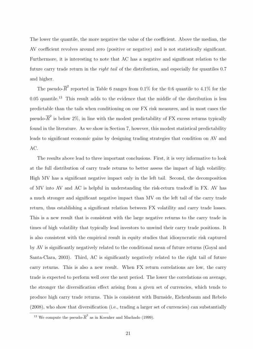
The lower the quantile, the more negative the value of the coefficient. Above the median, the

AV coefficient revolves around zero (positive or negative) and is not statistically significant.

Furthermore, it is interesting to note that AC has a negative and significant relation to the

future carry trade return in the right tail of the distribution, and especially for quantiles 0.7

and higher.

The pseudo-R2

reported in Table 6 ranges from 0.1% for the 0.6 quantile to 4.1% for the

0.05 quantile.13 This result adds to the evidence that the middle of the distribution is less

predictable than the tails when conditioning on our FX risk measures, and in most cases the

pseudo-R2

is below 2%, in line with the modest predictability of FX excess returns typically

found in the literature. As we show in Section 7, however, this modest statistical predictability

leads to significant economic gains by designing trading strategies that condition on AV and

AC.

The results above lead to three important conclusions. First, it is very informative to look

at the full distribution of carry trade returns to better assess the impact of high volatility.

High MV has a significant negative impact only in the left tail. Second, the decomposition

of MV into AV and AC is helpful in understanding the risk-return tradeoff in FX. AV has

a much stronger and significant negative impact than MV on the left tail of the carry trade

return, thus establishing a significant relation between FX volatility and carry trade losses.

This is a new result that is consistent with the large negative returns to the carry trade in

times of high volatility that typically lead investors to unwind their carry trade positions. It

is also consistent with the empirical result in equity studies that idiosyncratic risk captured

by AV is significantly negatively related to the conditional mean of future returns (Goyal and

Santa-Clara, 2003). Third, AC is significantly negatively related to the right tail of future

carry returns. This is also a new result. When FX return correlations are low, the carry

trade is expected to perform well over the next period. The lower the correlations on average,

the stronger the diversification effect arising from a given set of currencies, which tends to

produce high carry trade returns. This is consistent with Burnside, Eichenbaum and Rebelo

(2008), who show that diversification (i.e., trading a larger set of currencies) can substantially

13 We compute the pseudo-R2

as in Koenker and Machado (1999).

21

increase the Sharpe ratio of carry trade strategies.

In short, these results provide strong support in favor of the first testing hypothesis (H1 ):

AV and AC are more powerful predictors than MV for future carry returns. They also provide

partial support for the second testing hypothesis (H2 ): the predictive ability of AV and AC

is not the same across all quantiles, and in fact is stronger in the tails of the distribution.

However, in contrast to H2, we find that only AV has a significant negative effect in the left

tail, whereas AC has a significant negative effect in the right tail. This last result adds to

previous empirical evidence in that we show that the diversification benefit of low correlations

tends to have an asymmetric effect on the return distribution: AC significantly affects the

probability of large gains on carry trades, but its relation to large losses is insignificant. We

do not have a theoretical explanation for this asymmetric effect of AC, but believe that it is

an intriguing result that warrants further research.

5.4 Out-of-Sample Analysis

In addition to the in-sample analysis discussed above, we perform an out-of-sample exercise

that estimates a series of rolling predictive quantile regressions. We use a 20-year rolling

window (240 observations), which is sufficiently long to provide enough observations in each

quantile of the distribution. We then proceed forward by sequentially updating the parameter

estimates of the predictive quantile regressions month-by-month. We evaluate the performance

of the quantile regressions out of sample using the same criteria as for the in-sample analysis,

i.e., assessing whether the predictive ability is statistically significant by examining the slope

coefficients on AV and AC estimated using rolling regressions that condition only on available

information at the time the prediction of carry returns is made.

We plot the out-of-sample coefficients for AV and AC in Figure 5. For AV, the figure

displays the left-tail quantiles (0.1 to 0.5), whereas for AC the right-tail quantiles (0.5 to 0.9).

The figure illustrates that on average the time series of the out-of-sample coefficients have

similar values to the in-sample case. In other words, they tend to be negative and in most

cases become increasingly negative and increasingly statistically significant as we move away

from the median quantile. For AV, the most significant quantiles are the 0.2, 0.3 and 0.4.

22

Notably, at the 0.1 quantile, although negative, the coefficients are not significant for most

of the sample, which can be partly explained by the fact that this is the quantile with the

lowest number of observations. In short, the figure shows that, for each quantile, the size,

sign and significance of the coefficients tends to be fairly consistent over time and similar to

the in-sample results.14

5.5 Conditional Skewness

The carry trade return is well known to exhibit negative skewness due to large negative out-

liers.15 This has led to an emerging literature that investigates whether the high average carry

trade returns: (i) reflect a peso problem, which is the low probability of large negative outliers

(e.g., Burnside, Eichenbaum, Kleshchelski and Rebelo, 2011); and (ii) are compensation for

crash risk associated with the sudden unwinding of the carry trade (e.g., Brunnermeier, Nagel

and Pedersen, 2009; Farhi, Fraiberger, Gabaix, Ranciere and Verdelhan, 2009; and Jurek,

2009). In particular, Farhi et al. (2009) estimate the size of disaster risk premia and find that

they represent one-third of the carry trade return.

If crash risk is so fundamental in explaining the carry trade, we should observe large

negative conditional skewness. We investigate this further by exploiting an important ad-

vantage of our predictive quantile regression approach: it can be used to compute a measure

of conditional skewness that is robust to outliers. As in Kim and White (2004), we use the

Bowley (1920) coefficient of skewness that is based on the inter-quartile range. Using quantile

regression (27), we estimate skewness conditionally period-by-period as follows:

SKt =Q0.75,t + Q0.25,t − 2Q0.5,t

Q0.75,t − Q0.25,t

, (28)

where Q0.75,t is the forecast of the third conditional quartile at time t for next period, Q0.25,t is

the forecast of the first conditional quartile at time t for next period, and Q0.5,t is the forecast

14 In unreported results, we also compute the coverage ratios of the models as the percentage of times theactual returns fall below the predicted quantile. This shows, for example, whether 10% of the returns fallbelow the 0.1 quantile forecasts (see, e.g., Cenesizoglu and Timmermann, 2010). We find that the modelconditioning on AV and AC tends to perform well out of sample across quantiles.

15 Indeed, it is often said in industry speak that the carry trade payoffs “go up the stairs and down theelevator” or that the carry trade is like “picking up nickels in front of a steam roller.”

23

of the conditional median at time t for next period.

For any symmetric distribution, the Bowley coefficient is zero. This measure allows us to

explore whether an increase in total risk (e.g., a rise in average variance) typically coincides

with an increase in downside risk (e.g., lower conditional skewness). For example, when the

lower tail conditional quantiles decline more than the upper tail conditional quantiles, this

leads to negative conditional skewness and an increase in downside risk.

Figure 6 plots the conditional skewness and illustrates that, for most of our sample, it tends

to be low and positive but becomes highly negative during the recent financial crisis. Since

conditional skewness is not found to be consistently highly negative throughout the sample,

it seems unlikely that a peso problem or crash risk has been the key driver of the historically

high carry trade returns. This result is also consistent with Burnside et al. (2009), who do

not find statistically significant evidence of a peso problem over a similar sample period.

6 Robustness and Further Analysis

6.1 The Components of the Carry Trade

The carry trade return has two components: (i) the exchange rate component, which on

average is slightly negative for our sample; and (ii) the interest rate component, which on

average is highly positive.16 Note that the exchange rate component is the uncertain part of

the carry trade return as it is not known at the time that the carry trade portfolio is formed.

In contrast, the interest rate component is known and actually taken into account when the

carry trade portfolio is formed. Therefore, predicting the exchange rate component effectively

allows us to predict the carry trade return.

Figure 7 reports the results from estimating two quantile regressions, where on the left-

hand side we replace the carry returns with either the exchange rate component or the interest

rate component. The figure illustrates that when AV is high, the exchange rate component of

the carry trade exhibits large losses. This negative relation is highly significant for the left tail

of the exchange rate component up to the median, a result that is consistent with high-interest

16Recall the descriptive statistics in Table 2.

24

currencies depreciating sharply (i.e., the forward bias diminishing) when AV is high.17 More

importantly, this result also implies that to some extent exchange rates are predictable, which

constitutes evidence against the well-known finding that exchange rates follow a random walk.

In contrast, AV and AC have no impact on the interest rate component, which is not surprising

given that this component is known at the time of portfolio formation. To conclude, our results

establish that AV is a significant predictor of the large negative returns to the exchange rate

component of the carry trade.

6.2 Additional Predictive Variables

As a robustness test, we use two additional predictive variables to determine whether they

affect the significance of AV and AC. These are the average interest rate differential (AID)

and the lagged carry return (LCR). AID is equal to the average interest rate differential of the

quintile of currencies with the highest interest rates minus the average interest rate differential

of the quintile of currencies with the lowest interest rates. All interest rates are known at

time t for prediction of the carry trade return at time t + 1. LCR is simply the carry trade

return lagged by one month.

The predictive quantile regression results are in Figure 8 and Table 7, and can be summa-

rized in three findings: (i) AID has a significant positive effect on future carry trade returns in

the middle of the distribution;18 (ii) LCR has a significant positive effect in the left tail; and,

more importantly, (iii) the effect of AV and AC remains qualitatively the same (although their

significance diminishes slightly in the relevant parts of the distribution). For instance, the R2

now improves to 4.8% at the 0.05 quantile. Overall, the effect of AV and AC remains signifi-

cantly negative in the left and right tail, respectively, even when we include other significant

predictive variables.

17This case is also consistent with the hypothesis of flight to quality, safety (e.g., Ranaldo and Soderlind,2010) or liquidity that may explain why high-interest currencies depreciate and low-interest currencies appre-ciate in times of high volatility (Brunnermeier, Nagel and Pedersen, 2009).

18This result is consistent with Lustig, Roussanov and Verdelhan (2010), who find that the average forwarddiscount is a good predictor of FX excess returns. In their study, the average forward discount is equal to thedifference between the average interest of a basket of developed currencies and the US interest rate.

25

6.3 The Numeraire Effect

A unique feature of the FX market is that investors trade currencies but all exchange rates

are quoted relative to a numeraire. Consistent with the vast majority of the FX literature,

we use data on exchange rates relative to the US dollar. It is interesting, however, to check

whether using a different numeraire would meaningfully affect the predictive ability of AV and

AC. This is an important robustness check since it is straightforward to show analytically that

the carry trade returns and risk measures are not invariant to the numeraire.19 In essence,

the question we want to address is: given that changing the numeraire also changes the carry

returns and the risk measures, does the relation between risk and return also change?

We answer this question by reporting predictive quantile regression results using a compos-

ite numeraire that weighs the carry trade return, AV and AC across four different currencies.

The weights are based on the Special Drawing Rights (SDR) of the International Monetary

Fund (IMF) and are as follows: 41.9% on the US dollar-denominated measures, 37.4% on the

Euro-denominated measures, 11.3% on the UK pound-denominated measures, and 9.4% on

the Japanese yen-denominated measures. The SDR is an international reserve asset created

by the IMF in 1969 to supplement its member countries’ official reserves that is based on a

basket of these four key international currencies. The IMF (and other international organi-

zations) also use SDRs as a unit of account and effectively that is what we also do in this

exercise.

The advantage of this approach is that: (i) we capture the numeraire effect in a single

regression as opposed to estimating multiple regressions for each individual numeraire; (ii) it

is popular among practitioners who often measure FX returns using a composite numeraire

across these four main currencies;20 (iii) it provides the interpretation of generating a new

weighted carry trade portfolio; and (iv) the weighted AV and weighted AC are straightforward

19For example, consider taking the point of view of a European investor and hence changing the numerairefrom the US dollar to the euro. Then, all previous bilateral exchange rates become cross rates and Nt of theprevious cross rates become bilateral. Furthermore, converting dollar excess returns into euro excess returnsreplaces the US bond as the domestic asset by the European bond.

20Based on our experience, the typical weights adopted by practitioners in measuring returns relative to acomposite numeraire are: 40% on the US dollar, 30% on the euro, 20% on the Japanese yen and 10% on theUK pound.

26

to compute.21

The results shown in Figure 9 and Table 8 confirm that this exercise does not affect

qualitatively our main result: the weighted AV still has a significant negative effect on the

left tail of the future weighted carry trade return, and the weighted AC still has a significant

negative effect on the right tail. This is clear evidence that there is a strong statistical link

between average variance, average correlation and future carry returns for certain parts of the

distribution even when we consider a broad basket of numeraire currencies.

6.4 VIX, VXY and Carry Trade Returns

Our analysis quantifies FX risk using the risk measures of market variance, average variance

and average correlation. An alternative way of measuring risk is to use implied volatility (IV)

indices based on the IVs of traded options that can be thought of as the market’s expectation

of future realized volatility. As a further robustness check, we estimate predictive quantile

regressions using two IV indices: the VIX index, which is based on the 1-month model-free

IV of the S&P 500 equity index and is generally regarded as a measure of global risk appetite

(e.g., Brunnermeier, Nagel and Pedersen, 2009); and the VXY index, which is based on the

3-month IV of at-the-money forward options of the G-7 currencies. The sample period for the

VIX begins in January 1990 and for the VXY in January 1992, whereas for both it ends in

February 2009.

We begin with Table 9, which reports OLS results for simple contemporaneous regressions

of each of the two IV indices on MV, AV and AC. These results will help us determine the

extent to which the VIX and VXY are correlated with the FX risk measures we use. We

find that the VIX is significantly positively related to AV and significantly negatively related

to AC. Together AV and AC account for 37.6% of the variation of VIX. The VXY is also

significantly related to AV but the relation to AC is low and insignificant. AV accounts for

54.5% of the variation in VXY.

21The weighted carry trade return is computed as follows: rWC,t+1 =∑Pp=1 wprp,C,t+1, where p =

1, ...P = 4 is the number of numeraires. The weighted average variance is: AVWt+1 =∑Pp=1 wpAVp,t+1 =

1Nt

∑Nt

j=1

∑Pp=1 wpVp,j,t+1 for j currencies. The weighted average correlation is: ACWt+1 =

∑Pp=1 wpACp,t+1 =

1Nt(Nt−1)

∑Nt

i=1

∑Nt

j 6=i∑Pp=1 wpCp,ij,t+1 for i, j currencies.

27

The predictive quantile regression results for VIX and VXY, reported in Figure 10 and

Table 10, suggest that neither the VIX nor the VXY are significantly related to future carry

trade returns for any part of the distribution. Although the coefficients are predominantly

negative, there is no evidence of statistical significance. Therefore, the predictive ability of

AV and AC is not captured by the two IV indices and further justifies the choice of AV and

AC as risk measures. The lack of predictive ability for the VIX in one-month ahead predictive

regressions is consistent with the results of Brunnermeier, Nagel and Pedersen (2009), who

find that the VIX has a strong contemporaneous impact on the carry return but is not a

significant predictor.

6.5 AV and AC Measures Based on Intraday Returns

The monthly AV and AC measures we use throughout the analysis are based on daily FX

excess returns. In this robustness exercise, we assess whether our key results are affected

by estimating monthly AV and AC measures based on either 5-minute or 30-minute returns.

Specifically, we wish to determine how large is the measurement error in AV and AC due to

our use of daily, as opposed to high-frequency, data in the empirical analysis. Note that a

disadvantage of using high frequency data is that, due to lack of data availability, we inevitably

have to use a shorter sample and a much smaller cross section than the one used for the main

analysis. In particular, we use high frequency FX data from Olsen & Associates for eight

currencies relative to the US dollar. For six of the currencies, the sample starts on January 1,

1991: Australia, Canada, Euro area, Japan, Switzerland and the United Kingdom. For Sweden

it starts on January 1, 1997 and for New Zealand on January 1, 1998. For all currencies the

sample ends on February 28, 2009, which is the same end date as for the main analysis.

We construct spot rates on a five-minute grid for a 24-hour day using the nearest loga-

rithmic midquote price. The end of the day is defined as 16:00:00 GMT and the start as

16:05:00 GMT. We remove weekends defined as 16:05:00 Friday to 16:00:00 Sunday. Since

the dynamically rebalanced portfolio will be assessed from the point of view of a US investor,

we also remove US holidays and adjust for US daylight saving time. We construct 5-minute

and 30-minute intraday returns for computing the daily realized variances and covariances,

28

which are respectively the sums of squares or the sums of products of intraday returns. The

daily variances and covariances are aggregated to provide monthly realized measures, and

then averaged cross-sectionally to compute the average variance (AV) and average covariance

(ACOV). We use the monthly realized variances and covariances to compute the monthly re-

alized correlations, which are then averaged cross-sectionally to provide a measure of average

correlation (AC).22

Figure 11 displays the time series of AV, ACOV and AC, where each is constructed using

5-minute (5M) returns, 30-minute (30M) returns and daily (D) returns. The figure illustrates

that especially for AV and ACOV the measures move very closely across the three frequencies.

This is less the case for AC since monthly realized correlations are ratios based on estimates

of monthly realized covariances and (square roots of) realized variances. To be precise, the

correlations of the measures across frequencies are as follows:

• AV: Corr(5M,D) = 0.94; Corr(30M,D) = 0.98; and Corr(5M, 30M) = 0.97.

• ACOV: Corr(5M,D) = 0.93; Corr(30M,D) = 0.91; and Corr(5M, 30M) = 0.92.

• AC: Corr(5M,D) = 0.84; Corr(30M,D) = 0.79; and Corr(5M, 30M) = 0.86.

One would expect that more precise risk measures computed using high-frequency data

would provide more precise results in the estimation of the quantile regressions used to estab-

lish an intertemporal risk-return tradeoff. However, with the correlations ranging from 79%

to 98%, it is unlikely that the frequency of the data used to form the risk measures would

meaningfully affect our key results.23

7 Augmented Carry Trade Strategies

We further evaluate the predictive ability of average variance and average correlation on

22There is a large literature on modeling and forecasting realized variances and covariances. See, for example,Andersen, Bollerslev, Diebold and Labys (2003).

23However, we do not carry out this final test since if we were to estimate the quantile regressions usingmeasures based on intraday returns, we would be using a much shorter sample and smaller cross section. Thiswould not only affect the values of the risk measures, but it would also critically affect the composition ofthe carry trade portfolio as it would have to be based on much less currencies. This exercise would thereforesubstantially deviate from our main analysis, which relies on having a large cross section to build the carrytrade portfolio and risk measures.

29

future carry trade returns by assessing the economic gains of conditioning on average variance

and average correlation out of sample for three augmented carry trade strategies. These

strategies are then compared to the benchmark strategy, which is the standard carry trade.

Our discussion begins with a description of the strategies, then reports results with and

without transaction costs, and concludes by digging deeper into the composition of the carry

trade portfolio.

7.1 The Strategies

The first augmented carry trade strategy conditions only on AV and implements the following

rule at each time period t: for the carry trade returns that are lower than the τ -quantile of the

distribution, if AV has increased from t− 1 to t, we close the carry trade positions and thus

receive an excess return of zero at t+ 1; otherwise we execute the standard carry trade. This

strategy is designed to exploit the negative relation between current AV and the one-month

ahead carry return. In particular, it aims to avoid the low carry returns that follow high AV

when we are in the left tail. The focus of the AV strategy is the left-tail quantiles of the carry

trade return distribution because this is where the negative effect of AV is the strongest.

The second strategy conditions only on AC and implements the following rule at each

time period t: for the carry trade returns that are higher than the 1 − τ quantile, if AC has

decreased from t− 1 to t, we double the carry trade positions and thus receive twice the carry

return at t + 1; otherwise we execute the standard carry trade. This strategy is designed to

exploit the negative relation between current AC and the one-month ahead carry return. In

particular, it aims to take advantage of the high carry returns that follow low AC when we

are in the right tail. The focus of the AC strategy is the right-tail quantiles because this is

where the negative effect of AC is the strongest.

Third, the combined AV and AC strategy makes the following decision at each time period

t: for the carry trade returns that are lower than the τ -quantile, if AV has increased from

t− 1 to t, we close the carry trade positions and thus receive an excess return of zero at t+ 1;

and for the carry returns that are higher than the 1 − τ quantile, if AC has decreased from

t − 1 to t, we double the carry trade positions and thus receive twice the carry trade return

30

at t + 1; otherwise we execute the standard carry trade. The combined AV and AC strategy

focuses at the same time on both the low and the high quantiles of the carry trade return

distribution. For example, this strategy is first applied to the 0.1 (for AV) and 0.9 (for AC)

quantiles for the full sample, then to 0.2 and 0.8 quantiles and so on.

It is important to note that all three strategies are implemented out of sample. Specifically,

all strategies move forward recursively starting 3 years after the beginning of the sample.24

The strategies do not directly use the parameter estimates from the quantile regressions but

simply try to exploit the negative relation between future carry returns and current AV and

AC separately for low and high quantiles of the distribution.

The economic evaluation of the three strategies focuses on the Sharpe ratio. We also report

the mean and standard deviation of the augmented carry trade returns. All these measures

are reported in annualized units. We assess the practical applicability of the strategies by

computing the turnover ratio as the percentage of the currencies that on average are traded

every period. The turnover ratio provides us with a sense of how much more trading and

rebalancing is required to implement an augmented strategy relative to the standard carry

trade.

7.2 No Transaction Costs

Panel A of Table 11 reports the results for the case of no transaction costs. The AV strategy

performs very well for most quantiles and, as expected, does increasingly better as we move

to the lower quantiles. For example, at the 0.1 quantile, the Sharpe ratio of the AV strategy

is 1.314 compared to 1.070 for the standard carry trade. These large economic gains require

only slightly higher trading as the turnover ratio rises from 17.1% in the benchmark case to

20.8%. By design, the turnover ratio remains reasonably low for the lowest quantiles where

the conditioning on AV is implemented less often.

In contrast to the AV strategy that performs best in the lowest quantiles, the AC strategy

performs well across all quantiles. It appears, therefore, that low average correlations are

24Note that as a result of excluding the first three years of data, the statistics of the standard carry tradereturns reported in Table 11 differ slightly from those in Table 2.

31

economically beneficial to the carry trade regardless of the quantile we focus on. For example,

at the 0.1 quantile the Sharpe ratio of the AC strategy is 1.208, whereas at the 0.9 quantile

it is 1.134 compared to 1.070 of the standard carry trade. These economic gains require only

slightly higher trading for the high quantiles as the turnover ratio rises from 17.1% in the

benchmark case to 21.4% at the 0.9 quantile. By design, for the AC strategy the turnover

ratio remains reasonably low for the highest quantiles.

Finally, the combined AV and AC strategy performs better than the standard carry trade

for all quantiles. For example, at the highest and lowest quantiles (0.1 for AV and 0.9 for AC)

the Sharpe ratio is 1.224 and the turnover ratio is 0.257. In short, therefore, there are sizeable

economic gains in implementing augmented carry trade strategies that condition on average

variance and average correlation. In addition to showing tangible out-of-sample economic

gains, these results also highlight the negative predictive relation of AV and AC to future

carry trade returns across different quantiles of the distribution and provide further evidence

in full support of hypothesis H1 and partial support of hypothesis H2.

7.3 The Effect of Transaction Costs

A realistic assessment of the profitability of the carry trade strategies needs to account for

transaction costs in trading spot and forward exchange rates. Every month that we form a

new carry trade portfolio, we take a position in one forward and one spot contract for each

currency that belongs to either Portfolio 1 (highest interest rate currencies) or Portfolio 5

(lowest interest rate currencies). At the end of the month, the contracts expire and new

contracts are entered (on the same or different currencies). Define cSj,t and cFj,t as the one-way

proportional transaction cost at time t for trading at the spot and forward exchange rate

j, respectively. These values are equal to half of the spot and forward proportional bid-ask

spread.25 It is straightforward to show that the return to the carry trade for an individual

currency j net of transaction costs is equal to:

rnetj,t+1 = sj,t+1 − fj,t − cSj,t+1 − cFj,t. (29)

25The proportional bid-ask spread is the ratio of the bid-ask spread to the mid rate.

32

Our analysis implements the carry trade strategies using the transaction costs listed in

Table 1. Due to data availability, we use the median transaction costs across time, which

are different for each currency.26 These are taken from Datastream and are computed using

the longest bid and ask times series available for each exchange rate for the sample range of

January 1976 to February 2009. The cross-currency average of the median one-way transaction

costs is 6.10 basis points for the spot rates, and 9.42 basis points for the forward rates. Our

transaction costs are consistent with the values discussed in Neely, Weller and Ulrich (2009).

The performance of the carry trade strategies with transaction costs is shown in Panel

B of Table 11. As expected, when accounting for transaction costs the Sharpe ratios of

all strategies are lower. For example, the standard carry trade has a Sharpe ratio of 1.070

before transaction costs and 0.741 after transaction costs. More importantly, we find that the

augmented strategies still perform substantially better than the benchmark. In particular,

the AV strategy still dominates the standard carry trade in the left tail. The AC as well as

the combined AV and AC strategies outperform the benchmark in all quantiles. For example,

the AV strategy can deliver a Sharpe ratio net of transaction costs as high as 0.983, the AC

strategy as high as 0.971, and the combined strategy as high as 0.959, compared to 0.741 for

the benchmark. We conclude, therefore, that the improvement in the performance of the carry

trade when conditioning on the movements of AV and AC is robust to transaction costs.

7.4 Unpacking the Portfolios

The main finding of our empirical analysis is that, both from a statistical and an economic

perspective, AV has significant predictive ability in the left tail of the carry trade returns and

AC in the right tail. We look further into this finding by analyzing in detail the composition

of the two portfolios we use to form the carry trade: Portfolio 1 (high-interest currencies) and

26Using the median as opposed to the mean of transaction costs mitigates the effect of few large outliers inthe time series of bid-ask spreads. The results remain largely unchanged when using the mean proportionalbid-ask spread. Note also that generally the effective spread is lower than the quoted spread, since trading willtake place at the best price quoted at any point in time, suggesting that the worse quotes will not attract trades(e.g., Mayhew, 2002). Although some studies consider effective transaction costs in the range of 50% to 100%of the quoted spread (e.g., Goyal and Saretto, 2009), we use the full spread, which will likely underestimatethe actual returns.

33

Portfolio 5 (low-interest currencies). We focus on two cases: when AV increases and we are in

the 0.1 quantile; and when AC decreases and we are in the 0.9 quantile. This setup allows us

to unpack the portfolio results and thus understand better what drives the performance of the

standard and augmented carry trade strategies. We aim to answer the following questions:

Which currencies are included more frequently in the two portfolios used to form the carry

trade? Are they different in the left and right tail of the carry return distribution? Are there

common characteristics in the currencies selected in each of the two portfolios in terms of

geographical location, economic development and macroeconomic indicators? What is the

performance of these currencies and their sensitivity to AV and AC?

We answer these questions by focusing on the results of Table 12. At first glance, the table

shows that the composition of the two portfolios is rather diverse in terms of the characteristics

of the countries represented. For example, Portfolio 1 includes the currencies of South Africa,

New Zealand, Mexico, Italy and Portugal. These currencies remain in Portfolio 1 whether

we examine the left-tail or right-tail quantiles, the only exception being that Italy at the 0.1

quantile is replaced by Spain at the 0.9 quantile. It is evident that Portfolio 1 includes curren-

cies from four continents representing both emerging and developed economies. Regardless of

the geographic diversity, however, the main common characteristic of these currencies is that

they are from high-inflation countries. The average annual inflation rate for South Africa is

6.3%, for Mexico 8.3%, for Italy 9.4% and for Portugal 14.2%.27 The single exception is New

Zealand, which has an average inflation rate of 2.3%.28

We now turn to Portfolio 5, which includes the currencies of Japan, Switzerland, Singapore,

Germany and Hong Kong. These currencies also remain in Portfolio 5 whether we examine the

left-tail or right-tail quantiles, the only exception now being that Hong Kong at the 0.1 quantile

is replaced by Austria at the 0.9 quantile. Portfolio 5 includes currencies from Europe and Asia

27For the non-EU countries we use the common sample period of 1997Q1 to 2009Q1, for which all currenciesare available in our sample. The average inflation rates would be higher for these countries had we used earlierdata. For the European currencies that were replaced by the euro, we use the full sample before the adoptionof the euro: 1976Q1 to 1998Q4.

28Inflation in New Zealand was actually much higher in the 1970s and 1980s, before the Reserve Bank of NewZealand was the first central bank to adopt an explicit inflation targeting regime in 1990. Labuschagne andVowles (2010) show that the historically high interest rates of New Zealand relative to other OECD countriesare due to structurally low savings relative to investment, so that interest rates must be higher in New Zealandto keep inflation close to the central bank target.

34

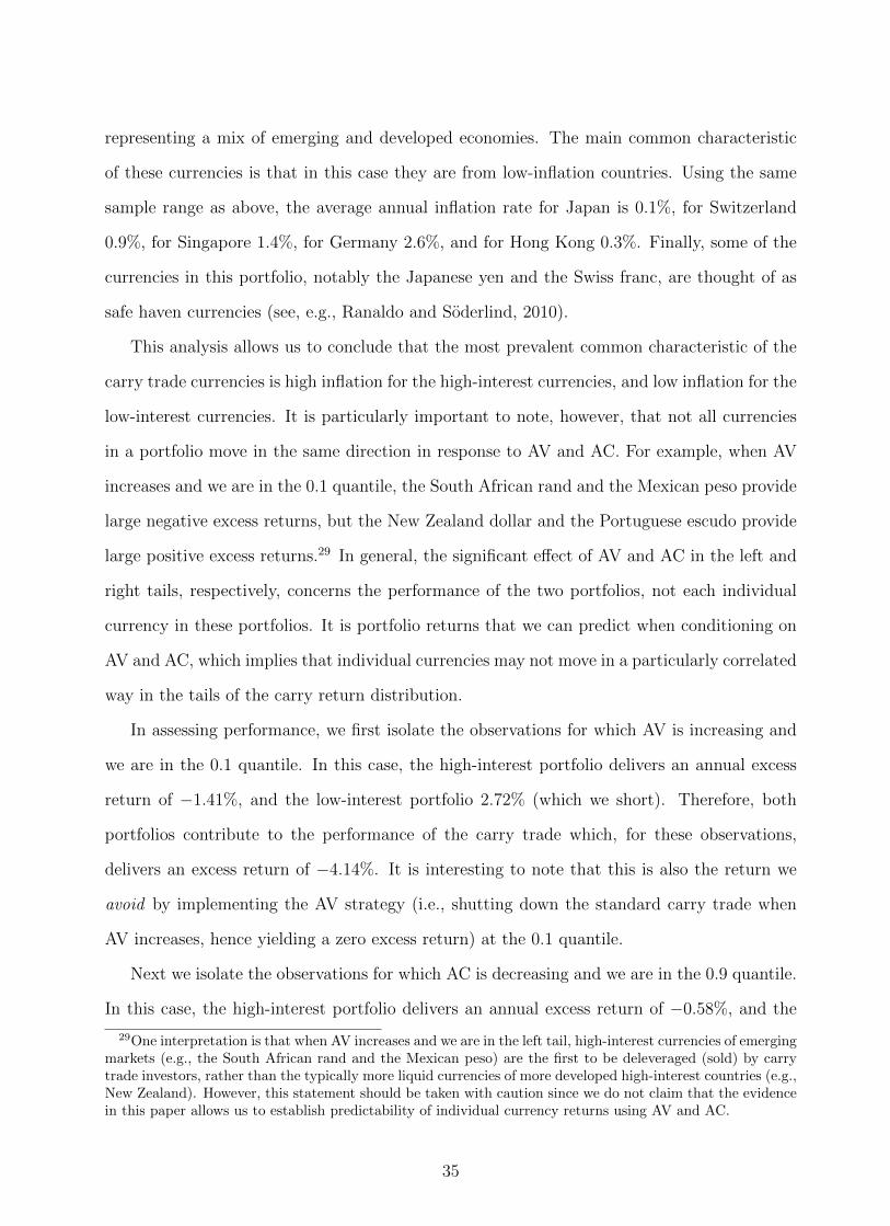
representing a mix of emerging and developed economies. The main common characteristic

of these currencies is that in this case they are from low-inflation countries. Using the same

sample range as above, the average annual inflation rate for Japan is 0.1%, for Switzerland

0.9%, for Singapore 1.4%, for Germany 2.6%, and for Hong Kong 0.3%. Finally, some of the

currencies in this portfolio, notably the Japanese yen and the Swiss franc, are thought of as

safe haven currencies (see, e.g., Ranaldo and Soderlind, 2010).

This analysis allows us to conclude that the most prevalent common characteristic of the

carry trade currencies is high inflation for the high-interest currencies, and low inflation for the

low-interest currencies. It is particularly important to note, however, that not all currencies

in a portfolio move in the same direction in response to AV and AC. For example, when AV

increases and we are in the 0.1 quantile, the South African rand and the Mexican peso provide

large negative excess returns, but the New Zealand dollar and the Portuguese escudo provide

large positive excess returns.29 In general, the significant effect of AV and AC in the left and

right tails, respectively, concerns the performance of the two portfolios, not each individual

currency in these portfolios. It is portfolio returns that we can predict when conditioning on

AV and AC, which implies that individual currencies may not move in a particularly correlated

way in the tails of the carry return distribution.

In assessing performance, we first isolate the observations for which AV is increasing and

we are in the 0.1 quantile. In this case, the high-interest portfolio delivers an annual excess

return of −1.41%, and the low-interest portfolio 2.72% (which we short). Therefore, both

portfolios contribute to the performance of the carry trade which, for these observations,

delivers an excess return of −4.14%. It is interesting to note that this is also the return we

avoid by implementing the AV strategy (i.e., shutting down the standard carry trade when

AV increases, hence yielding a zero excess return) at the 0.1 quantile.

Next we isolate the observations for which AC is decreasing and we are in the 0.9 quantile.

In this case, the high-interest portfolio delivers an annual excess return of −0.58%, and the

29One interpretation is that when AV increases and we are in the left tail, high-interest currencies of emergingmarkets (e.g., the South African rand and the Mexican peso) are the first to be deleveraged (sold) by carrytrade investors, rather than the typically more liquid currencies of more developed high-interest countries (e.g.,New Zealand). However, this statement should be taken with caution since we do not claim that the evidencein this paper allows us to establish predictability of individual currency returns using AV and AC.

35

low-interest portfolio −9.17% (which we short).30 Therefore, the good performance of the

carry trade in the right tail of 8.59% (= −0.58% + 9.17%) is almost exclusively due to the

shorting (i.e., borrowing in) low interest currencies. Note that this carry return of 8.59%

also indicates the return we double by implementing the AC strategy (i.e., doubling up the

standard carry trade when AC decreases) at the 0.9 quantile.

Finally, the movement of AV and AC does not seem to be highly correlated in either the

left or the right tail. When AV increases in the left tail, AC increases only 43% of the time,

whereas when AC decreases in the right tail, AV decreases only 55% of the time. Hence,

for example, when AV increases and large negative returns follow, this is not likely to be

associated with an increase in AC. This confirms the quantile regression result that only AV

affects carry returns in the left tail, and only AC affects carry returns in the right tail.

8 Conclusion

The carry trade is a currency investment strategy designed to exploit deviations from uncov-

ered interest parity. Its profitability is based on the empirical observation that the interest

rate differential across countries is not, on average, offset by a depreciation of the investment

currency. Hence, investing in high-interest currencies by borrowing in low-interest currencies

tends to deliver large positive excess returns.

This paper fills a gap in the literature by demonstrating empirically the existence of an

intertemporal risk-return tradeoff between the return to the carry trade and risk in a predictive

setting. We measure FX risk by the variance of the returns to the FX market portfolio. We

then take a step further by decomposing the market variance into the cross-sectional average

variance and the cross-sectional average correlation of exchange rate returns. Our empirical

analysis is based on predictive quantile regressions, which provide a natural way of assessing

the effect of higher risk on different quantiles of the return distribution.

Our main finding is that average variance has a significant negative effect on the left tail

of the distribution of future carry trade returns, whereas average correlation has a significant

30The large return of−9.17% of the low-interest portfolio is to some extent due to the interest rate componentof the low interest currencies (−3.14%), but mostly due to their exchange rate component (−6.03%).

36

negative effect on the right tail. We take advantage of this finding by forming a new version

of the carry trade that conditions on average variance and average correlation, and show that

this strategy performs considerably better than the standard carry trade. These results imply

that to some extent exchange rates are predictable, especially when it matters most: when

the carry trade produces large gains or large losses. In other words, if the carry trade is about

“going up the stairs and down the elevator,” then average variance and average correlation

can tell us something valuable about when the elevator is likely to go up or down. In the end,

by focusing on the tails of the return distribution of carry trades, we uncover a significantly

negative risk-return tradeoff in foreign exchange.

37

A Appendix: Notes on the bootstrap procedure

A.1 Bootstrap Standard Errors

We estimate the standard error of the parameters of the predictive quantile regressions using a

moving block bootstrap (MBB), which provides inference that is robust to heteroskedasticity

and autocorrelation of unknown form (Fitzenberger, 1997). Specifically, we employ a circular

MBB of the model residuals as in Politis and Romano (1992). The optimal block size is

selected using the automatic procedure of Politis and White (2004), as amended by Patton,

Politis and White (2009). The bootstrap algorithm implements the following steps:

1. Estimate the coefficients of the τ -th conditional quantile function:

Qyt+1(τ | Xt) = X ′tβ(τ),

for t = 1, . . . , T , where yt+1 is the dependent variable (e.g., the carry trade return), Xt is

a K×1 matrix of regressors (e.g., a constant, AV and AC), and β(τ) is the K×1 vector

of coefficients. We denote the estimates as β(τ) and obtain the residuals associated with

the τ -th quantile as εt+1 = yt+1 −X ′tβ(τ).

2. “Wrap” the residuals {ε1, . . . , εT} around a circle, i.e., define the new series et = εt for

t = 1, . . . , T , and et = εt−T for t = T + 1, . . . , T + l − 1, where l is the length of the

block defined below. This “circular” structure, specified by Politis and Romano (1992),

guarantees that the first and last few observations have the same probability of being

selected as observations in the middle of the series.

3. Construct a bootstrap pseudo-series {e∗1, . . . , e∗T} by resampling with replacement of

overlapping blocks of size l. The block size l is computed using the automatic procedure

of Politis and White (2004). In our application, the estimated optimal block length

ranges from 1 to 4 monthly observations.

4. Form the dependent variable y∗t+1 using the bootstrap residual series e∗ ≡ {e∗1, . . . , e∗T}′

38

and the estimates β(τ) as follows:

y∗t+1 = X ′tβ(τ) + e∗t+1,

and then estimate the conditional quantile function Qy∗t+1(τ | Xt) = X ′tβ(τ), obtaining

the bootstrap estimate β∗(τ).

5. Repeat steps 3 and 4 for B = 10, 000 times. Denoting β∗j(τ) as the estimate of the jth

bootstrap, for j = 1, . . . , B, estimate the variance-covariance matrix of β(τ) as follows:

Var(β(τ)

)=

1

B

B∑j=1

(β∗j(τ)− β∗j(τ)

)(β∗j(τ)− β∗j(τ)

)′.

A.2 Bootstrap Hypothesis Testing

In order to test the null hypothesis of no predictability (i.e., β(τ) = 0), we perform a double

bootstrap to compute the bootstrap p-values (see, e.g., MacKinnon, 2007). The procedure is

as follows:

I. Obtain the estimate β(τ).

II. Obtain the estimate Var(β(τ)

)using the block bootstrap described above for B2 = 500

bootstrap samples.

III. Compute the t-statistic for each coefficient βi(τ), i = 1, ..., K as follows:

ti =βi(τ)√

Var(βi(τ)

) .

IV. Generate B1 = 1, 000 bootstrap samples using the bootstrap DGP as in step 4 above,

but this time imposing the null βi(τ) = 0. Use each of the new samples to calculate

β∗∗i,j(τ), j = 1, . . . , B1.

39

V. For each of the B1 bootstrap samples, perform steps II and III above in order to generate

B1 bootstrap test statistics t∗∗i,j.

VI. Calculate the bootstrap p-values for ti using

p∗i (ti) =1

B1

B1∑j=1

I(|t∗∗i,j| > |ti|),

where I(·) denotes the indicator function, which is equal to 1 when its argument is true

and 0 otherwise.

40

Table 1. Exchange Rates

The table lists the 33 US dollar nominal exchange rates used to construct the FX market and carry

trade portfolios. The start date and end date of the data sample is shown for each exchange rate. The

transaction costs reported below are the median one-way proportional costs for the spot and forward exchange

rates, defined as half of the bid-ask spread divided by the mid rate, and are reported in basis points. The

transaction costs are computed using the longest bid and ask times series available for each exchange rate for

the sample range of January 1976 to February 2009.

Transaction Costs

Exchange Rate Start of Sample End of Sample Spot Forward

1 Australian Dollar December 1984 February 2009 5.42 7.31

2 Austrian Schilling January 1976 December 1998 7.64 11.08

3 Belgian Franc January 1976 December 1998 7.92 12.67

4 Canadian Dollar January 1976 February 2009 2.72 4.75

5 Czech Koruna January 1997 February 2009 5.97 6.75

6 Danish Krone January 1976 February 2009 4.16 7.03

7 Euro January 1999 February 2009 2.64 2.77

8 Finnish Markka January 1997 December 1998 6.52 5.28

9 French Franc January 1976 December 1998 4.98 7.56

10 German Mark January 1976 December 1998 8.09 15.55

11 Greek Drachma January 1997 December 2000 4.07 5.45

12 Hong Kong Dollar October 1983 February 2009 0.64 1.92

13 Hungarian Forint October 1997 February 2009 5.05 8.36

14 Indian Rupee October 1997 February 2009 3.13 4.39

15 Irish Punt January 1976 December 1998 4.70 9.00

16 Italian Lira January 1976 December 1998 3.16 8.54

17 Japanese Yen June 1978 February 2009 10.32 9.76

18 Mexican Peso January 1997 February 2009 4.35 5.25

19 Netherlands Guilder January 1976 December 1998 11.71 17.21

20 New Zealand Dollar December 1984 February 2009 8.14 10.44

21 Norwegian Krone January 1976 February 2009 4.65 7.29

22 Philippine Peso January 1997 February 2009 13.61 15.85

23 Polish Zloty February 2002 February 2009 6.52 7.41

24 Portuguese Escudo January 1976 December 1998 18.76 34.43

25 Saudi Arabian Riyal January 1997 February 2009 0.53 0.93

26 Singaporean Dollar December 1984 February 2009 3.14 6.94

27 South African Rand October 1983 February 2009 11.46 20.12

28 South Korean Won February 2002 February 2009 2.24 6.44

29 Spanish Peseta January 1976 December 1998 6.98 12.08

30 Swedish Krona January 1976 February 2009 4.85 7.76

31 Swiss Franc January 1976 February 2009 11.61 18.60

32 Taiwanese Dollar January 1997 February 2009 2.95 8.28

33 United Kingdom Pound January 1976 February 2009 2.67 3.54

41

Table 2. Descriptive Statistics

The table reports descriptive statistics for the monthly excess returns of two FX portfolios: the carry tradeand the market; for the two components of the carry trade: the exchange rate depreciation and the interest ratedifferential; and for three monthly risk measures: market variance, average variance and average correlation.The sample of 33 US dollar nominal exchange rates runs from January 1976 to February 2009. The return tothe FX market portfolio is an equally weighted average of all exchange rate excess returns. The carry tradeportfolio is constructed every month by going long on the quintile of currencies with the highest interest ratesand going short on the bottom quintile. Market variance is the variance of the monthly returns to the FXmarket portfolio. Average variance is the equally weighted cross-sectional average of the monthly variancesof all exchange rate excess returns. Average correlation is the equally weighted cross-sectional average ofthe pairwise monthly correlations of all exchange rate excess returns. The mean, standard deviation and theSharpe ratio are annualized and assume no transaction costs. AR(1) is the first order autocorrelation.

Panel A: Summary Statistics

Mean St. Dev. Sharpe Ratio Skewness Kurtosis AR(1)Portfolio Returns

Carry Trade 0.086 0.078 1.092 −0.967 6.043 0.132Market 0.010 0.078 0.131 −0.120 3.195 0.097

Carry Trade ComponentsExchange Rate −0.051 0.079 −1.133 6.232 0.140Interest Rate 0.137 0.023 2.506 15.578 0.655

Variances and CorrelationsMarket Variance 0.005 0.002 3.380 19.367 0.512Average Variance 0.010 0.003 5.174 47.780 0.539Average Correlation 0.477 0.182 0.028 2.241 0.796

Panel B: Cross-Correlations

Carry Market Market Average AverageReturn Return Variance Variance Correlation

Portfolio ReturnsCarry Trade Return 1.000Market Return 0.091 1.000

Variances and CorrelationsMarket Variance −0.250 −0.145 1.000Average Variance −0.371 −0.150 0.877 1.000Average Correlation −0.048 −0.054 0.478 0.191 1.000

42

Table 3. Market Variance Decomposition

The table presents the ordinary least squares results for regressions on alternative decompositions of the

FX market variance. The dependent variable is the market variance defined as the variance of the monthly

returns to the FX market portfolio, which is an equally weighted average of the excess returns of 33 US dollar

nominal spot exchange rates. Average variance is the equally weighted cross-sectional average of the variances

of all exchange rate excess returns. Average correlation is the equally weighted cross-sectional average of

the pairwise correlations of all exchange rate excess returns. All variables are contemporaneous and, with

the exception of average correlation, they are annualized. Newey-West (1987) t-statistics with five lags are

reported in parentheses. The sample period runs from of January 1976 to February 2009.

Regressions for the Market Variance

(1) (2) (3) (4)Constant 0.000 −0.002 −0.004 0.000

(0.056) (−2.324) (−11.079) (1.473)

Average Variance 0.493 0.456(9.993) (13.883)

Average Correlation 0.015 0.010(8.960) (13.784)

(Average Variance)×(Average Correlation)

0.939(24.281)

R2

(%) 76.8 23.5 86.8 93.0

43

Table 4. OLS Predictive Regressions

The table presents the ordinary least squares results for two predictive regressions. The first regression

is: rC,t+1 = α + βMVt + εt+1, where rC,t+1 is the one-month ahead carry trade return and MVt is the

lagged market variance. The second regression is: rC,t+1 = α + β1AVt + β2ACt + εt+1, where AVt is the

lagged average variance and ACt is the lagged average correlation. The return to the carry trade portfolio

is constructed every month by going long on the quintile of currencies with the highest interest rates and

going short on the bottom quintile. Market variance is the variance of the return to the market portfolio

constructed as the equally weighted average of the excess returns on 33 US dollar nominal exchange rates.

Average variance is the equally weighted cross-sectional average of the monthly variances of all exchange rate

excess returns. Average correlation is the equally weighted cross-sectional average of the pairwise monthly

correlations of all exchange rate excess returns. With the exception of average correlation, all variables are

annualized. Newey-West (1987) t-statistics with five lags are reported in parentheses. Bootstrap p-values

generated using 10,000 bootstrap samples are in brackets. The sample period runs from of January 1976 to

February 2009.

Regressions for the Carry Trade Return

(1) (2)Constant 0.115 0.156

(5.939) (3.888)[0.122] [0.064]

Market Variance −5.999(−2.006)[0.046]

Average Variance −3.781(−1.972)[0.051]

Average Correlation −0.070(−0.936)[0.350]

R2

(%) 1.2 1.8

44

Table 5. Market Variance

The table presents the regression results for the conditional quantile function: QrC,t+1(τ |MVt) = α (τ) + β (τ)MVt, where τ is a quantile of the

one-month ahead carry trade return rC,t+1 and MVt is the lagged market variance. The return to the carry trade portfolio is constructed every month by

going long on the quintile of currencies with the highest interest rates and going short on the bottom quintile. Market variance is the variance of the return

to the market portfolio constructed as the equally weighted average of the excess return on 33 US dollar nominal exchange rates. All variables are annualized.

Bootstrap t-statistics generated using 1,000 bootstrap samples are reported in parentheses. Bootstrap p-values using the double bootstrap are in brackets. The

pseudo-R2

is computed as in Koenker and Machado (1999). The sample period runs from of January 1976 to February 2009.

Predictive Quantile Regressions for the Carry Trade Return

Quantile 0.05 0.1 0.2 0.3 0.4 0.5 0.6 0.7 0.8 0.9 0.95

Constant −0.024 −0.019 −0.005 0.003 0.007 0.011 0.015 0.020 0.025 0.034 0.044

(−6.227) (−4.742) (−2.100) (1.424) (4.711) (7.297) (8.886) (10.660) (17.106) (15.022) (15.569)

[0.000] [0.001] [0.058] [0.169] [0.001] [0.000] [0.000] [0.000] [0.000] [0.000] [0.000]

Market Variance −23.709 −4.473 −6.514 −6.691 −5.885 −5.358 −4.017 −3.206 −2.835 −5.588 −8.031

(−3.256) (−0.731) (−1.577) (−2.265) (−2.364) (−2.192) (−1.533) (−1.139) (−1.109) (−1.546) (−1.598)

[0.006] [0.495] [0.120] [0.042] [0.035] [0.039] [0.147] [0.296] [0.259] [0.132] [0.137]

R2

(%) 0.9 0.4 0.4 0.8 1.1 0.5 −0.1 0.0 0.3 0.7 0.8

45

Table 6. Average Variance and Average Correlation

The table presents the regression results for the conditional quantile function: QrC,t+1(τ | AVt, ACt) = α (τ) + β1 (τ)AVt + β2 (τ)ACt, where τ is

a quantile of the one-month ahead carry trade return rC,t+1, AVt is the lagged average variance and ACt is the lagged average correlation. The return to

the carry trade portfolio is constructed every month by going long on the quintile of currencies with the highest interest rates and going short on the bottom

quintile. Average variance is the equally weighted cross-sectional average of the monthly variances of all exchange rate excess returns. Average correlation is

the equally weighted cross-sectional average of the pairwise monthly correlations of all exchange rate excess returns. With the exception of average correlation,

all variables are annualized. Bootstrap t-statistics generated using 1,000 bootstrap samples are reported in parentheses. Bootstrap p-values using the double

bootstrap are in brackets. The pseudo-R2

is computed as in Koenker and Machado (1999). The sample period runs from of January 1976 to February 2009.

Predictive Quantile Regressions for the Carry Trade Return

Quantile 0.05 0.1 0.2 0.3 0.4 0.5 0.6 0.7 0.8 0.9 0.95

Constant −0.017 −0.009 −0.005 0.004 0.010 0.014 0.020 0.025 0.032 0.040 0.055

(−2.246) (−0.988) (−1.125) (1.064) (3.349) (4.686) (6.116) (8.705) (10.367) (8.833) 9.383

[0.041] [0.406] [0.287] [0.317] [0.004] [0.000] [0.000] [0.000] [0.000] [0.000] [0.000]

Average Variance −12.727 −9.538 −6.558 −5.971 −4.250 −2.059 −2.616 0.223 −0.960 0.194 −3.603

(−3.242) (−3.165) (−2.865) (−3.572) (−3.087) (−1.551) (−1.713) (0.159) (−0.603) (0.102) (−1.338)

[0.014] [0.008] [0.008] [0.001] [0.007] [0.127] [0.095] [0.862] [0.538] [0.913] [0.191]

Average Correlation −0.010 −0.010 0.007 0.001 −0.003 −0.008 −0.009 −0.015 −0.015 −0.019 −0.023

(−0.662) (−0.616) (0.726) (0.130) (−0.603) (−1.329) (−1.362) (−2.601) (−2.310) (−2.141) (−2.084)

[0.496] [0.613] [0.474] [0.894] [0.557] [0.164] [0.233] [0.016] [0.031] [0.051] [0.080]

R2

(%) 4.1 1.0 0.9 1.1 1.2 0.6 0.1 0.8 0.9 1.6 1.8

46

Table 7. Additional Predictive Variables

The table presents the regression results for the conditional quantile function: QrC,t+1(τ | AVt, ACt, AIDt, rC,t) = α (τ) + β1 (τ)AVt + β2 (τ)ACt +

β3 (τ)AIDt + β4 (τ) rC,t, where τ is a quantile of the one-month ahead carry trade return rC,t+1, AVt is the lagged average variance, ACt is the lagged

average correlation, AIDt is the average interest rate differential and rC,t is the lagged carry trade return. The return to the carry trade portfolio is constructed

every month by going long on the quintile of currencies with the highest interest rates and going short on the bottom quintile. Average variance is the equally

weighted cross-sectional average of the monthly variances of all exchange rate excess returns. Average correlation is the equally weighted cross-sectional average

of the pairwise monthly correlations of all exchange rate excess returns. AID is the average interest rate differential of the quintile of currencies with the highest

interest rates minus the average interest rate differential of the quintile of currencies with the lowest interest rates. With the exception of average correlation,

all variables are annualized. Bootstrap t-statistics generated using 1,000 bootstrap samples are reported in parentheses. Bootstrap p-values using the double

bootstrap are in brackets. The pseudo-R2

is computed as in Koenker and Machado (1999). The sample period runs from of January 1976 to February 2009.

Predictive Quantile Regressions for the Carry Trade Return

Quantile 0.05 0.1 0.2 0.3 0.4 0.5 0.6 0.7 0.8 0.9 0.95

Constant −0.013 −0.015 −0.009 −0.003 0.003 0.007 0.012 0.019 0.028 0.037 0.054

(−1.521) (−2.008) (−1.562) (−0.695) (1.075) (2.303) (3.176) (5.515) (7.979) (8.012) (7.882)

[0.162] [0.100] [0.185] [0.554] [0.252] [0.036] [0.007] [0.000] [0.000] [0.000] [0.000]

Average Variance −10.434 −5.689 −5.958 −5.457 −3.704 −4.086 −2.063 −2.720 −1.874 −0.735 −2.868

(−2.568) (−1.752) (−2.472) (−3.018) (−2.499) (−2.819) (−1.394) (−1.808) (−1.136) (−0.334) (−0.946)

[0.028] [0.090] [0.033] [0.007] [0.022] [0.010] [0.204] [0.079] [0.248] [0.736] [0.382]

Average Correlation −0.014 −0.012 −0.002 0.003 −0.004 −0.003 −0.006 −0.010 −0.016 −0.019 −0.026

(−0.972) (−0.961) (−0.181) (0.380) (−0.800) (−0.489) (−1.061) (−1.727) (−2.597) (−2.396) (−2.125)

[0.336] [0.428] [0.866] [0.722] [0.401] [0.611] [0.327] [0.102] [0.028] [0.039] [0.081]

Average Interest Differential −0.398 0.218 0.519 0.463 0.499 0.443 0.440 0.502 0.403 0.226 0.040

(−0.936) (0.583) (1.946) (2.372) (3.295) (2.978) (2.466) (3.032) (2.515) (0.956) (0.128)

[0.331] [0.622] [0.083] [0.042] [0.000] [0.007] [0.023] [0.004] [0.027] [0.339] [0.905]

Lagged Carry Return 0.255 0.296 0.154 0.101 0.089 0.067 0.035 0.015 −0.043 0.013 0.048

(1.892) (2.722) (2.002) (1.686) (1.953) (1.461) (0.663) (0.300) (−0.810) (0.193) (0.476)

[0.084] [0.021] [0.060] [0.128] [0.051] [0.153] [0.553] [0.749] [0.431] [0.853] [0.692]

R2

(%) 4.8 3.1 2.1 2.4 2.9 2.0 1.1 1.6 1.1 1.6 1.4

47

Table 8. Weighted Average Variance and Weighted Average Correlation

The table presents the regression results for the conditional quantile function: QrWC,t+1

(τ | AV W

t , ACWt)

= α (τ) + β1 (τ)AV Wt + β2 (τ)ACWt , where

τ is a quantile of the one-month ahead weighted carry trade return rWC,t+1, AV Wt is the lagged weighted average variance and ACWt is the lagged weighted

average correlation. All variables are weighted in order to account for the effect of numeraire in both the carry trade return and the risk measures. The weights

are based on the Special Drawing Rights (SDR) of the International Monetary Fund and are as follows: 41.9% on the US dollar-denominated measures, 37.4%

on the Euro-denominated measures, 11.3% on the UK pound-denominated measures and 9.4% on the Japanese yen-denominated measures. The weighted

return to the carry trade portfolio uses the SDR weights across the four numeraires, and for a given numeraire is constructed every month by going long on

the quintile of currencies with the highest interest rates and going short on the bottom quintile. Weighted average variance is the weighted average across

the four numeraires, where for a given numeraire average variance is the equally weighted cross-sectional average of the monthly variances of all exchange rate

excess returns. Weighted average correlation is the weighted average across the four numeraires, where for a given numeraire average correlation is the equally

weighted cross-sectional average of the pairwise monthly correlations of all exchange rate excess returns. With the exception of average correlation, all variables

are annualized. Bootstrap t-statistics generated using 1,000 bootstrap samples are reported in parentheses. Bootstrap p-values using the double bootstrap are

in brackets. The pseudo-R2

is computed as in Koenker and Machado (1999). The sample period runs from of January 1976 to February 2009.

Predictive Quantile Regressions for the Weighted Carry Trade Return

Quantile 0.05 0.1 0.2 0.3 0.4 0.5 0.6 0.7 0.8 0.9 0.95

Constant −0.024 −0.015 −0.009 0.003 0.014 0.018 0.026 0.037 0.041 0.053 0.060

(−1.781) (−1.011) (−1.151) (0.438) (2.742) (3.717) (4.449) (7.676) (7.786) (6.618) 5.114

[0.074] [0.398] [0.237] [0.650] [0.016] [0.001] [0.000] [0.000] [0.000] [0.000] [0.000]

Weighted Ave. Variance −13.230 −14.365 −6.793 −6.619 −4.924 −3.755 −2.663 −1.633 −1.916 −1.560 −1.273

(−3.216) (−4.174) (−2.856) (−3.418) (−2.985) (−2.407) (−1.718) (−1.131) (−1.189) (−0.747) (−0.430)

[0.013] [0.007] [0.011] [0.006] [0.013] [0.028] [0.093] [0.227] [0.211] [0.420] [0.723]

Weighted Ave. Correlation 0.004 0.011 0.017 0.004 −0.012 −0.016 −0.024 −0.038 −0.038 −0.048 −0.045

(0.143) (0.331) (0.923) (0.304) (−1.033) (−1.485) (−1.834) (−3.622) (−3.210) (−2.768) (−1.741)

[0.846] [0.786] [0.335] [0.735] [0.306] [0.143] [0.081] [0.001] [0.008] [0.008] [0.162]

R2

(%) 4.4 1.8 1.1 1.0 1.1 0.7 0.6 1.4 1.7 1.4 1.0

48

Table 9. VIX, VXY and FX Risk Measures

The table presents ordinary least squares results for regressions of the VIX and VXY indices on monthly

FX risk measures. The VIX index is based on the 1-month model-free implied volatility of the S&P 500 equity

index. The VXY index is based on the 3-month implied volatility of at-the-money-forward options on the G-7

currencies. Market variance is the variance of the return to the market portfolio constructed as the equally

weighted average of the excess returns on 33 US dollar nominal exchange rates. Average variance is the equally

weighted cross-sectional average of the variances of exchange rate excess returns. Average correlation is the

equally weighted cross-sectional average of the pairwise correlations of exchange rate excess returns. With the

exception of average correlation, all variables are annualized. Newey-West (1987) t-statistics with five lags are

reported in parentheses. The sample period for the VIX begins in January 1990 and for the VXY in January

1992. The sample period for all indices ends in February 2009.

Panel A: Regressions for the VIX

(1) (2) (3) (4) (5)Constant 0.014 0.013 0.021 0.019 0.015

(13.962) (17.851) (16.058) (15.103) (15.302)

Market Variance 5.695(2.113)

Average Variance 3.556 4.003(6.559) (7.729)

Average Correlation −0.012 −0.016(−3.862) (−5.113)

(Average Variance)×(Average Correlation)

5.496(2.159)

R2

(%) 13.5 24.7 6.9 37.6 12.4

Panel B: Regressions for the VXY

Constant 0.008 0.007 0.008 0.008 0.008(35.786) (30.391) (19.371) (19.868) (35.791)

Market Variance 3.305(10.540)

Average Variance 1.462 1.473(7.142) (6.869)

Average Correlation 0.001 −0.001(1.269) (−0.519)

(Average Variance)×(Average Correlation)

3.201(9.628)

R2

(%) 53.0 54.5 0.5 54.4 49.6

49

Table 10. VIX and VXY

The table presents the regression results for two conditional quantile functions. The first one is: QrC,t+1(τ | V IXt) = α (τ) + β (τ)V IXt, where τ is a

quantile of the one-month ahead carry trade return rC,t+1 and V IXt is the lagged VIX index. The second one is: QrC,t+1(τ | V XYt) = α (τ) + β (τ)V XYt,

where V XYt is the lagged VXY index. The return to the carry trade portfolio is constructed every month by going long on the quintile of currencies with the

highest interest rates and going short on the bottom quintile. The VIX index is based on the 1-month model-free implied volatility of the S&P 500 equity index.

The VXY index is based on the 3-month implied volatility of at-the-money-forward options on the G-7 currencies. All variables are annualized. Bootstrap

t-statistics generated using 1,000 bootstrap samples are reported in parentheses. Bootstrap p-values using the double bootstrap are in brackets. The pseudo-R2

is computed as in Koenker and Machado (1999). The sample period runs from of January 1976 to February 2009.

Panel A: The Carry Trade Return on VIX

Quantile 0.05 0.1 0.2 0.3 0.4 0.5 0.6 0.7 0.8 0.9 0.95

Constant −0.018 −0.021 −0.004 0.004 0.004 0.009 0.014 0.016 0.019 0.025 0.023

(−1.382) (−1.875) (−0.507) (0.686) (0.929) (2.013) (3.670) (3.576) (4.077) (3.972) (3.521)

[0.195] [0.097] [0.621] [0.464] [0.359] [0.090] [0.003] [0.006] [0.003] [0.001] [0.006]

VIX −0.103 −0.027 −0.023 −0.018 0.006 0.008 −0.001 0.015 0.023 0.026 0.070

(−1.620) (−0.511) (−0.580) (−0.605) (0.283) (0.379) (−0.029) (0.731) (1.057) (0.870) (1.988)

[0.140] [0.605] [0.584] [0.511] [0.745] [0.699] [0.957] [0.520] [0.341] [0.444] [0.065]

R2

(%) 0.8 −0.2 −0.2 −0.3 −0.4 −0.4 −0.4 −0.2 0.2 0.1 2.1

Panel B: The Carry Trade Return on VXY

Constant −0.051 −0.028 0.003 0.009 0.012 0.023 0.028 0.039 0.027 0.041 0.024

(−1.646) (−1.660) (0.241) (0.953) (1.347) (2.379) (3.239) (4.258) (3.093) (4.029) (1.414)

[0.150] [0.098] [0.795] [0.356] [0.199] [0.028] [0.004] [0.001] [0.010] [0.003] [0.173]

VXY 0.183 0.073 −0.096 −0.102 −0.082 −0.123 −0.140 −0.190 0.005 −0.081 0.160

(0.628) (0.447) (−0.777) (−1.139) (−0.959) (−1.354) (−1.704) (−2.209) (0.061) (−0.828) (0.956)

[0.591] [0.615] [0.439] [0.282] [0.355] [0.185] [0.105] [0.044] [0.916] [0.373] [0.352]

R2

(%) −0.2 −0.2 0.1 0.1 0.4 1.0 1.0 0.4 −0.5 −0.3 1.2

50

Table 11. Out-of-Sample Augmented Carry Trade Strategies

The table presents the out-of-sample performance of augmented carry trade strategies that condition on

the movement of average variance and/or average correlation with and without transaction costs. Panel A

assumes no transaction costs, whereas Panel B implements the carry trade strategies using the transaction costs

listed in Table 1. Average variance is the equally weighted cross-sectional average of the monthly variances

of all exchange rate excess returns. The average variance strategy implements the following rule at each time

t : for the carry trade returns that are lower than the τ -quantile of the distribution, if average variance has

increased from t-1 to t, we close the carry trade positions and thus receive a return of zero at t+1; otherwise

we execute the standard carry trade. Average correlation is the equally weighted cross-sectional average of the

pairwise monthly correlations of all exchange rate excess returns. The average correlation strategy implements

the following rule at each time t : for the carry trade returns that are higher than the 1−τ quantile, if average

correlation has decreased from t-1 to t, we double the carry trade positions and thus receive twice the carry

return at t+1; otherwise we execute the standard carry trade. The combined average variance and average

correlation strategy makes the following decision at each time t : for the carry trade returns that are lower

than the τ -quantile, if average variance has increased from t-1 to t, we close the carry trade positions and

thus receive a return of zero; and for the carry trade returns that are higher than the 1−τ quantile, if average

correlation has decreased from t-1 to t, we double the carry trade positions and thus receive twice the carry

return; otherwise we execute the standard carry trade. The mean, standard deviation and Sharpe ratio are

reported in annualized terms. The turnover ratio is equal to the percentage of the currencies that on average

are traded every month. The sample period runs from of January 1976 to February 2009. All strategies

move forward recursively starting 3 years after the beginning of the sample so that the first observation is for

January 1979.

Panel A: No Transaction Costs

Carry Trade Average Variance StrategyQuantile 0.1 0.2 0.3 0.4 0.5 0.6 0.7 0.8 0.9Mean 0.084 0.094 0.091 0.085 0.079 0.073 0.069 0.066 0.059 0.054St. Dev. 0.079 0.071 0.069 0.066 0.065 0.064 0.061 0.060 0.057 0.056Sharpe ratio 1.070 1.314 1.326 1.279 1.213 1.142 1.120 1.098 1.022 0.968Turnover 0.171 0.208 0.264 0.310 0.346 0.387 0.421 0.444 0.485 0.514

Average Correlation StrategyMean 0.084 0.146 0.147 0.139 0.130 0.122 0.118 0.114 0.107 0.097St. Dev. 0.079 0.121 0.115 0.111 0.107 0.104 0.100 0.096 0.091 0.085Sharpe ratio 1.070 1.208 1.284 1.262 1.212 1.174 1.186 1.186 1.182 1.134Turnover 0.171 0.557 0.511 0.454 0.412 0.370 0.340 0.294 0.252 0.214

Combined Average Variance and Average Correlation StrategyMean 0.084 0.104 0.106 0.107 0.106 0.099St. Dev. 0.079 0.095 0.092 0.088 0.084 0.081Sharpe ratio 1.070 1.095 1.152 1.211 1.264 1.224Turnover 0.171 0.589 0.522 0.440 0.352 0.257

(continued)

51

Panel B: With Transaction Costs

Carry Trade Average Variance StrategyQuantile 0.1 0.2 0.3 0.4 0.5 0.6 0.7 0.8 0.9Mean 0.058 0.070 0.068 0.062 0.058 0.055 0.053 0.050 0.043 0.040St. Dev. 0.079 0.071 0.069 0.066 0.065 0.063 0.061 0.060 0.057 0.055Sharpe ratio 0.741 0.977 0.983 0.941 0.892 0.866 0.869 0.836 0.761 0.729Turnover 0.171 0.208 0.259 0.306 0.344 0.385 0.417 0.442 0.485 0.513

Average Correlation StrategyMean 0.058 0.109 0.109 0.107 0.097 0.091 0.090 0.085 0.079 0.070St. Dev. 0.079 0.121 0.115 0.111 0.107 0.103 0.099 0.095 0.090 0.085Sharpe ratio 0.741 0.903 0.949 0.971 0.913 0.881 0.904 0.891 0.876 0.823Turnover 0.171 0.557 0.513 0.458 0.411 0.375 0.341 0.296 0.252 0.215

Combined Average Variance and Average Correlation StrategyMean 0.058 0.081 0.082 0.081 0.080 0.074St. Dev. 0.079 0.094 0.091 0.088 0.084 0.081Sharpe ratio 0.741 0.853 0.895 0.926 0.959 0.914Turnover 0.171 0.594 0.521 0.438 0.347 0.259

52

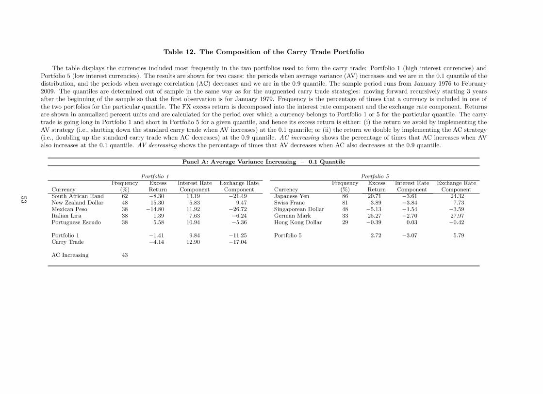
Table 12. The Composition of the Carry Trade Portfolio

The table displays the currencies included most frequently in the two portfolios used to form the carry trade: Portfolio 1 (high interest currencies) andPortfolio 5 (low interest currencies). The results are shown for two cases: the periods when average variance (AV) increases and we are in the 0.1 quantile of thedistribution, and the periods when average correlation (AC) decreases and we are in the 0.9 quantile. The sample period runs from January 1976 to February2009. The quantiles are determined out of sample in the same way as for the augmented carry trade strategies: moving forward recursively starting 3 yearsafter the beginning of the sample so that the first observation is for January 1979. Frequency is the percentage of times that a currency is included in one ofthe two portfolios for the particular quantile. The FX excess return is decomposed into the interest rate component and the exchange rate component. Returnsare shown in annualized percent units and are calculated for the period over which a currency belongs to Portfolio 1 or 5 for the particular quantile. The carrytrade is going long in Portfolio 1 and short in Portfolio 5 for a given quantile, and hence its excess return is either: (i) the return we avoid by implementing theAV strategy (i.e., shutting down the standard carry trade when AV increases) at the 0.1 quantile; or (ii) the return we double by implementing the AC strategy(i.e., doubling up the standard carry trade when AC decreases) at the 0.9 quantile. AC increasing shows the percentage of times that AC increases when AValso increases at the 0.1 quantile. AV decreasing shows the percentage of times that AV decreases when AC also decreases at the 0.9 quantile.

Panel A: Average Variance Increasing – 0.1 Quantile

Portfolio 1 Portfolio 5Frequency Excess Interest Rate Exchange Rate Frequency Excess Interest Rate Exchange Rate

Currency (%) Return Component Component Currency (%) Return Component ComponentSouth African Rand 62 −8.30 13.19 −21.49 Japanese Yen 86 20.71 −3.61 24.32New Zealand Dollar 48 15.30 5.83 9.47 Swiss Franc 81 3.89 −3.84 7.73Mexican Peso 38 −14.80 11.92 −26.72 Singaporean Dollar 48 −5.13 −1.54 −3.59Italian Lira 38 1.39 7.63 −6.24 German Mark 33 25.27 −2.70 27.97Portuguese Escudo 38 5.58 10.94 −5.36 Hong Kong Dollar 29 −0.39 0.03 −0.42

Portfolio 1 −1.41 9.84 −11.25 Portfolio 5 2.72 −3.07 5.79Carry Trade −4.14 12.90 −17.04

AC Increasing 43

53

Panel B: Average Correlation Decreasing – 0.9 Quantile

Portfolio 1 Portfolio 5Frequency Excess Interest Rate Exchange Rate Frequency Excess Interest Rate Exchange Rate

Currency (%) Return Component Component Currency (%) Return Component ComponentPortuguese Escudo 64 −2.17 16.43 −18.60 Japanese Yen 86 −1.63 −3.61 1.98South African Rand 55 26.38 38.24 −11.83 Swiss Franc 82 −12.25 −3.94 −8.31New Zealand Dollar 45 3.45 11.16 −7.71 German Mark 45 −14.63 −3.69 −10.94Spanish Peseta 36 2.94 8.17 −5.23 Singaporean Dollar 41 12.83 −1.66 14.49Mexican Peso 32 −3.37 7.43 −10.80 Austrian Schilling 32 6.54 −3.27 9.81

Portfolio 1 −0.58 13.93 −14.51 Portfolio 5 −9.17 −3.14 −6.03Carry Trade 8.59 17.08 −8.49

AV Decreasing 55

54

1975 1980 1985 1990 1995 2000 2005 20100

0.5

1

1.5

2

2.5

3

3.5

4

4.5

5Cumulative Carry Trade Return

1975 1980 1985 1990 1995 2000 2005 20100

0.1

0.2

0.3

0.4

0.5

0.6

0.7

0.8

0.9Average Correlation

1975 1980 1985 1990 1995 2000 2005 20100

0.02

0.04

0.06

0.08

0.1

0.12

0.14Average Variance

1980 1985 1990 1995 2000 2005 2010−0.2

−0.1

0

0.1

0.2

0.3

0.4

0.5

0.6

0.7Rolling Correlation Between AV and AC

Figure 1. Carry Trade Return, Average Variance and Average Correlation

This figure displays the time series of the cumulative carry trade return (top left), FX average variance (topright), FX average correlation (bottom left) and the rolling correlation between average variance and averagecorrelation using a 5-year rolling window (bottom right). The sample ranges from January 1976 to February2009.

55

1975 1980 1985 1990 1995 2000 2005 2010−2

−1

0

1Carry Return < 0.1−quantile vs. AV

1975 1980 1985 1990 1995 2000 2005 20100

0.05

0.1

0.15

1975 1980 1985 1990 1995 2000 2005 20100

0.05

0.1

0.15

1975 1980 1985 1990 1995 2000 2005 2010−2

−1

0

1Carry Return < 0.1−quantile vs. AC

1975 1980 1985 1990 1995 2000 2005 20100

0.2

0.4

0.6

0.8

1

1975 1980 1985 1990 1995 2000 2005 20100

0.2

0.4

0.6

0.8

1

1975 1980 1985 1990 1995 2000 2005 2010−2

−1

0

1Carry Return > 0.9−quantile vs. AV

1975 1980 1985 1990 1995 2000 2005 20100

0.05

0.1

0.15

1975 1980 1985 1990 1995 2000 2005 20100

0.05

0.1

0.15

1975 1980 1985 1990 1995 2000 2005 2010

−1

0

1Carry Return > 0.9−quantile vs. AC

1975 1980 1985 1990 1995 2000 2005 20100

0.2

0.4

0.6

0.8

1

1975 1980 1985 1990 1995 2000 2005 20100

0.2

0.4

0.6

0.8

1

Figure 2. Carry Return Quantiles versus Average Variance and Average Correlation

This figure plots the carry trade return against AV (top) and AC (bottom) and identifies with dots two cases:the carry trade return observations belonging to the 0.1 quantile (left); and the carry trade return observationsbelonging to the 0.9 quantile (right). The return quantiles here are determined unconditionally by sorting thereturn observations over the full sample.

56

0.050.1 0.2 0.3 0.4 0.5 0.6 0.7 0.8 0.90.95−0.04

−0.03

−0.02

−0.01

0

0.01

0.02

0.03

0.04

0.05Constant

Quantile

α

0.050.1 0.2 0.3 0.4 0.5 0.6 0.7 0.8 0.90.95−40

−35

−30

−25

−20

−15

−10

−5

0

5

10Market Variance

Quantile

β

Figure 3. Market Variance

This figure shows the parameter estimates of the predictive quantile regression of the one-month-ahead carrytrade return on the lagged market variance. The dashed lines indicate the 95% confidence interval based onbootstrap standard errors.

57

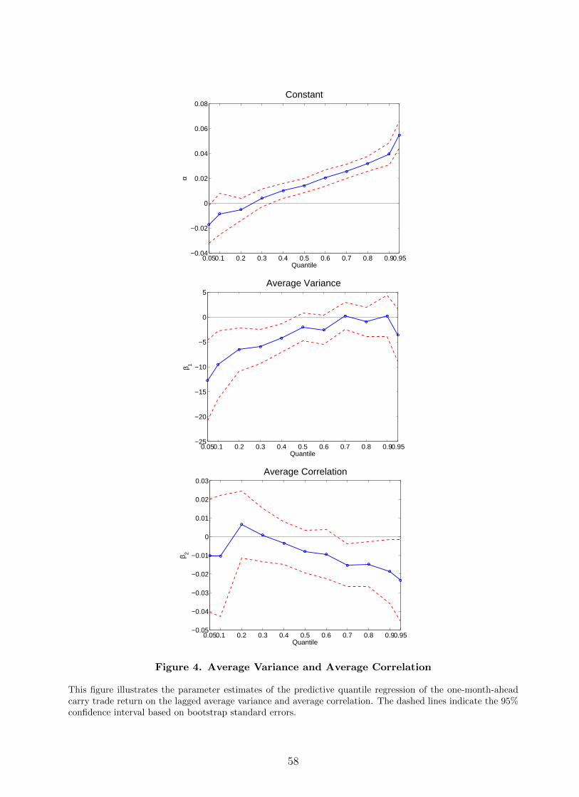
0.050.1 0.2 0.3 0.4 0.5 0.6 0.7 0.8 0.90.95−0.04

−0.02

0

0.02

0.04

0.06

0.08Constant

Quantile

α

0.050.1 0.2 0.3 0.4 0.5 0.6 0.7 0.8 0.90.95−25

−20

−15

−10

−5

0

5Average Variance

Quantile

β 1

0.050.1 0.2 0.3 0.4 0.5 0.6 0.7 0.8 0.90.95−0.05

−0.04

−0.03

−0.02

−0.01

0

0.01

0.02

0.03Average Correlation

Quantile

β 2

Figure 4. Average Variance and Average Correlation

This figure illustrates the parameter estimates of the predictive quantile regression of the one-month-aheadcarry trade return on the lagged average variance and average correlation. The dashed lines indicate the 95%confidence interval based on bootstrap standard errors.

58

1995 2000 2005 2010−25

−20

−15

−10

−5

0

5

10AV Coefficient, q = 0.1

1995 2000 2005 2010−25

−20

−15

−10

−5

0

5AV Coefficient, q = 0.2

1995 2000 2005 2010−18

−16

−14

−12

−10

−8

−6

−4

−2

0AV Coefficient, q = 0.3

1995 2000 2005 2010−18

−16

−14

−12

−10

−8

−6

−4

−2

0

2AV Coefficient, q = 0.4

1995 2000 2005 2010−14

−12

−10

−8

−6

−4

−2

0

2

4

6AV Coefficient, q = 0.5

1995 2000 2005 2010−0.04

−0.03

−0.02

−0.01

0

0.01

0.02

0.03

0.04AC Coefficient, q = 0.5

1995 2000 2005 2010−0.05

−0.04

−0.03

−0.02

−0.01

0

0.01

0.02

0.03AC Coefficient, q = 0.6

1995 2000 2005 2010−0.05

−0.04

−0.03

−0.02

−0.01

0

0.01

0.02

0.03AC Coefficient, q = 0.7

1995 2000 2005 2010−0.06

−0.05

−0.04

−0.03

−0.02

−0.01

0

0.01

0.02

0.03AC Coefficient, q = 0.8

1995 2000 2005 2010−0.08

−0.07

−0.06

−0.05

−0.04

−0.03

−0.02

−0.01

0

0.01

0.02AC Coefficient, q = 0.9

Figure 5. Out-of-Sample Quantile Regression Coefficients

This figure plots the out-of-sample predictive quantile regression coefficients for average variance and averagecorrelation. For average variance, the figure displays the left-tail quantiles (0.1 to 0.5), whereas for averagecorrelation the right-tail quantiles (0.5 to 0.9). The out-of-sample regressions use a 20-year rolling window(240 observations).

59

1975 1980 1985 1990 1995 2000 2005 2010−0.4

−0.3

−0.2

−0.1

0

0.1

0.2

0.3

Figure 6. Conditional Skewness

This figure shows the time-variation of the robust conditional skewness measure of Kim and White (2004)based on the predictive quantile regressions. The measure uses the inter-quartile range.

60

0.050.1 0.2 0.3 0.4 0.5 0.6 0.7 0.8 0.90.95−0.06

−0.04

−0.02

0

0.02

0.04

0.06

Exchange Rate Component:Constant

Quantile

α

0.050.1 0.2 0.3 0.4 0.5 0.6 0.7 0.8 0.90.95−25

−20

−15

−10

−5

0

5

Exchange Rate Component:Average Variance

Quantile

β 1

0.050.1 0.2 0.3 0.4 0.5 0.6 0.7 0.8 0.90.95−0.05

0

0.05

Exchange Rate Component:Average Correlation

Quantile

β 2

0.050.1 0.2 0.3 0.4 0.5 0.6 0.7 0.8 0.90.950

0.005

0.01

0.015

0.02

0.025

0.03

0.035

0.04

0.045

Interest Rate Component:Constant

Quantile

α

0.050.1 0.2 0.3 0.4 0.5 0.6 0.7 0.8 0.90.95−3

−2

−1

0

1

2

3

4

5

Interest Rate Component:Average Variance

Quantile

β 1

0.050.1 0.2 0.3 0.4 0.5 0.6 0.7 0.8 0.90.95−0.05

−0.04

−0.03

−0.02

−0.01

0

0.01

0.02

Interest Rate Component:Average Correlation

Quantile

β 2

Figure 7. The Exchange Rate and Interest Rate Components of the Carry Trade

This figure exhibits the parameter estimates of two sets of predictive quantile regressions. The left panel showsthe results for the one-month-ahead exchange rate component of the carry trade return on the lagged averagevariance and lagged average correlation. The right panel shows the results for the interest rate component ofthe carry trade return on the lagged average variance and average correlation. The dashed lines indicate the95% confidence interval based on bootstrap standard errors.

61

0.050.1 0.2 0.3 0.4 0.5 0.6 0.7 0.8 0.90.95−0.04

−0.02

0

0.02

0.04

0.06

0.08Constant

Quantile

α

0.050.1 0.2 0.3 0.4 0.5 0.6 0.7 0.8 0.90.95−20

−15

−10

−5

0

5Average Variance

Quantile

β 1

0.050.1 0.2 0.3 0.4 0.5 0.6 0.7 0.8 0.90.95−0.05

−0.04

−0.03

−0.02

−0.01

0

0.01

0.02Average Correlation

Quantile

β 2

0.050.1 0.2 0.3 0.4 0.5 0.6 0.7 0.8 0.90.95−1.5

−1

−0.5

0

0.5

1

1.5Interest differential

Quantile

β 3

0.050.1 0.2 0.3 0.4 0.5 0.6 0.7 0.8 0.90.95−0.2

−0.1

0

0.1

0.2

0.3

0.4

0.5

0.6Lagged Carry Return

Quantile

β 4

Figure 8. Additional Predictive Variables

This figure illustrates the parameter estimates of the predictive quantile regression of the one-month-aheadcarry trade return on the lagged average variance, lagged average correlation and two additional predictivevariables: the interest rate differential and the lagged carry trade return. The dashed lines indicate the 95%confidence interval based on bootstrap standard errors.

62

0.050.1 0.2 0.3 0.4 0.5 0.6 0.7 0.8 0.90.95−0.06

−0.04

−0.02

0

0.02

0.04

0.06

0.08Constant

Quantile

α

0.050.1 0.2 0.3 0.4 0.5 0.6 0.7 0.8 0.90.95−25

−20

−15

−10

−5

0

5

10Weighted Average Variance

Quantile

β 1

0.050.1 0.2 0.3 0.4 0.5 0.6 0.7 0.8 0.90.95−0.1

−0.08

−0.06

−0.04

−0.02

0

0.02

0.04

0.06

0.08Weighted Average Correlation

Quantile

β 2

Figure 9. The Numeraire Effect

This figure displays the parameter estimates of the predictive quantile regression of the weighted one-month-ahead carry trade return on the lagged weighted average variance and lagged weighted average correlation.The weighted variables account for the numeraire effect using the IMF weights for Special Drawing Rights:41.9% on the US dollar, 37.4% on the Euro, 11.3% on the UK pound and 9.4% on the Japanese yen. Thedashed lines indicate the 95% confidence interval based on bootstrap standard errors.

63

0.050.1 0.2 0.3 0.4 0.5 0.6 0.7 0.8 0.90.95−0.05

−0.04

−0.03

−0.02

−0.01

0

0.01

0.02

0.03

0.04Constant

Quantile

α

0.050.1 0.2 0.3 0.4 0.5 0.6 0.7 0.8 0.90.95−0.25

−0.2

−0.15

−0.1

−0.05

0

0.05

0.1

0.15VIX

Quantile

β

0.050.1 0.2 0.3 0.4 0.5 0.6 0.7 0.8 0.90.95−0.12

−0.1

−0.08

−0.06

−0.04

−0.02

0

0.02

0.04

0.06

0.08Constant

Quantile

α

0.050.1 0.2 0.3 0.4 0.5 0.6 0.7 0.8 0.90.95−0.6

−0.4

−0.2

0

0.2

0.4

0.6

0.8VXY

Quantile

β

Figure 10. VIX and VXY

This figure exhibits the parameter estimates of two sets of predictive quantile regressions. The left panel showsthe results for the one-month-ahead carry trade return on the lagged VIX index. The right panel shows theresults for the one-month-ahead carry trade return on the lagged VXY index. The dashed lines indicate the95% confidence interval based on bootstrap standard errors.

64

1990 1995 2000 2005 20100

0.02

0.04

0.06

0.08

0.1

0.12

0.14Average Variance

AV−5MinAV−30MinAV−Daily

1990 1995 2000 2005 2010−0.005

0

0.005

0.01

0.015

0.02

0.025

0.03

0.035

0.04Average Covariance

ACOV−5MinACOV−30MinACOV−Daily

1990 1995 2000 2005 20100

0.1

0.2

0.3

0.4

0.5

0.6

0.7

0.8

0.9

1Average Correlation

AC−5MinAC−30MinAC−Daily

Figure 11. Average Variance, Average Covariance and Average Correlation using In-traday Returns

This figure displays the time series of average variance (AV), average covariance (ACOV) and average cor-relation (AC), where each is constructed using 5-minute returns, 30-minute returns and daily returns. Themeasures are computed using a sample consisting of eight currencies relative to the US dollar. For six curren-cies, the sample starts on January 1, 1991: Australia, Canada, Euro area, Japan, Switzerland and the UnitedKingdom. For Sweden it starts on January 1, 1997 and for New Zealand on January 1, 1998. For all currenciesthe sample ends on February 28, 2009. 65

References

Akram, Q.F., D. Rime, and L. Sarno (2008). “Arbitrage in the Foreign Exchange Market:

Turning on the Microscope,” Journal of International Economics 76, 237–253.

Andersen, T.G., T. Bollerslev, F.X. Diebold, and P. Labys (2003). “Modeling and Forecasting

Realized Volatility,” Econometrica 71, 579–625.

Ang, A., R.J. Hodrick, Y. Xing, and X. Zhang (2006). “The Cross-Section of Volatility and

Expected Returns,” Journal of Finance 61, 259–299.

Ang, A., R.J. Hodrick, Y. Xing, and X. Zhang (2009). “High Idiosyncratic Volatility and

Low Returns: International and Further U.S. Evidence,” Journal of Financial Economics 91,

1–23.

Bali, T.G. (2008). “The Intertemporal Relation between Expected Returns and Risk,” Journal

of Financial Economics 87, 101–131.

Bali, T.G., N. Cakici, X. Yan, and Z. Zhang (2005). “Does Idiosyncratic Risk Really Matter?”

Journal of Finance 60, 905–929.

Bali, T.G., and K. Yilmaz (2012). “The Intertemporal Relation between Expected Return and

Risk on Currency,” Handbook of Financial Econometrics and Statistics, ed. C.-F. Lee. New

York: Springer (forthcoming).

Bandi, F.M., and B. Perron (2008). “Long-Run Risk-Return Trade-offs,” Journal of Econo-

metrics 143, 349–374.

Bekaert, G., (1995). “The Time Variation of Expected Returns and Volatility in Foreign

Exchange Markets,” Journal of Business and Economic Statistics 13, 397–408.

Bilson, J.F.O. (1981). “The ‘Speculative Efficiency’ Hypothesis,” Journal of Business 54,

435–451.

Bowley, A.L. (1920). Elements of Statistics. Scribner’s: New York.

66

Brandt, M.W., and Q. Kang (2004). “On the Relationship between the Conditional Mean and

Volatility of Stock Returns: A Latent VAR Approach,” Journal of Financial Economics 72,

217–257.

Brunnermeier, M.K., S. Nagel, and L.H. Pedersen (2009). “Carry Trades and Currency

Crashes,” NBER Macroeconomics Annual 2008, 313–347.

Brunnermeier, M.K. and L.H. Pedersen (2009). “Market Liquidity and Funding Liquidity,”

Review of Financial Studies 22, 2201-2238.

Burnside, C. (2012). “Carry Trades and Risk,” in James, J., L. Sarno and I.W. Marsh (eds.)

Handbook of Exchange Rates. Hoboken, New Jersey, US: John Wiley & Sons.

Burnside, C., M. Eichenbaum, I. Kleshchelski, and S. Rebelo (2011). “Do Peso Problems

Explain the Returns to the Carry Trade?” Review of Financial Studies 24, 853–891.

Burnside, C., M. Eichenbaum, and S. Rebelo (2008). “Carry Trade: The Gains of Diversifi-

cation,” Journal of the European Economic Association 6, 581–588.

Cenesizoglu, T., and A. Timmermann (2010). “Do Return Prediction Models Add Economic

Value?” Unpublished Working Paper, HEC Montreal.

Chan, Y.L., and L. Kogan (2002). “Catching up with the Joneses: Heterogeneous Preferences

and the Dynamics of Asset Prices,” Journal of Political Economy 110, 1255–1285.

Chan, K.C., G.A. Karolyi, and R.M. Stulz (1992). “Global Financial Markets and the Risk

Premium on U.S. Equity,” Journal of Financial Economics 32, 137–167.

Chen, Z., and R. Petkova (2011). “Does Idiosyncratic Volatility Proxy for Risk Exposure?”

Unpublished Working Paper, Texas A&M University.

Christiansen, C. (2011). “Intertemporal Risk-Return Trade-Off in Foreign Exchange Rates,”

Journal of International Financial Markets, Institutions and Money 21, 535–549.

Christiansen, C., A. Ranaldo, and P. Soderlind (2011). “The Time-Varying Systematic Risk

of Carry Trade Strategies,”Journal of Financial and Quantitative Analysis 46, 1107–1125.

67

Constantinides, G.M. (2002). “Rational Asset Prices,” Journal of Finance 57, 1567–1591.

Constantinides, G.M., and D. Duffie (1996). “Asset Pricing with Heterogeneous Consumers,”

Journal of Political Economy 104, 219–240.

Della Corte, P., L. Sarno, and I. Tsiakas (2009). “An Economic Evaluation of Empirical

Exchange Rate Models,” Review of Financial Studies 22, 3491–3530.

Diebold, F.X., and M. Nerlove (1989). “The Dynamics of Exchange Rate Volatility: A Mul-

tivariate Latent Factor ARCH Model,” Journal of Applied Econometrics 4, 1–21.

Engel, C. (1996). “The Forward Discount Anomaly and the Risk Premium: A Survey of

Recent Evidence,” Journal of Empirical Finance 3, 123–192.

Fama, E.F. (1984). “Forward and Spot Exchange Rates,” Journal of Monetary Economics 14,

319–338.

Fama, E.F., and K. French (1993). “Common Risk Factors in the Returns on Stocks and

Bonds,” Journal of Financial Economics 33, 3–56.

Farhi, E., S.P. Fraiberger, X. Gabaix, R. Ranciere, and A. Verdelhan (2009). “Crash Risk in

Currency Markets,” Unpublished Working Paper, Harvard University.

Fitzenberger, B., (1997). “The Moving Block Bootstrap and Robust Inference for Linear Least

Squares and Quantile Regressions,” Journal of Econometrics 82, 235–287.

French, K.R., W. Schwert, and R.F. Stambaugh (1987). “Expected Stock Returns and Volatil-

ity,” Journal of Financial Economics 19, 3–29.

Ghysels, E., P. Santa-Clara, and R. Valkanov (2005). “There is a Risk-Return Trade-off After

All,” Journal of Financial Economics 76, 509–548.

Glosten, L.R., R. Jagannathan, and D.E. Runkle (1993). “On the Relationship Between the

Expected Value and the Volatility of the Nominal Excess Return on Stocks,” Journal of

Finance 48, 1779–1801.

68

Goyal A., and P. Santa-Clara (2003). “Idiosyncratic Risk Matters!” Journal of Finance 58,

975–1007.

Goyal, A., and A. Saretto (2009). “Cross-Section of Option Returns and Volatility,” Journal

of Financial Economics 94, 310–326.

Jurek, J., (2009). “Crash-Neutral Currency Carry Trades,” Unpublished Working Paper,

Princeton University.

Kim, T-H., and H. White (2004). “On More Robust Estimation of Skewness and Kurtosis,”

Finance Research Letters 1, 56–73.

Koenker, R. (2005). Quantile Regression. New York: Cambridge University Press.

Koenker, R., and J. Machado (1999). “Goodness of Fit and Related Inference Processes for

Quantile Regression,” Journal of the American Statistical Association 94, 1296–1310.

Krishnan, C.N.V., R. Petkova, and P. Ritchken (2009). “Correlation Risk,” Journal of Em-

pirical Finance 16, 353–367.

Labuschagne, N., and P. Vowles (2010). “Why are Real Interest Rates in New Zealand so

High? Evidence and Drivers,” New Zealand Treasury Working Paper 10/09.

Lustig, H., N. Roussanov, and A. Verdelhan (2010). “Countercyclical Currency Risk Premia,”

Unpublished Working Paper, MIT.

Lustig, H., N. Roussanov, and A. Verdelhan (2011). “Common Risk Factors in Currency

Markets,” Review of Financial Studies 24, 3731–3777.

MacKinnon, J., (2007). “Bootstrap Hypothesis Testing,” QED Working Paper No. 1127.

Mancini-Griffoli, T., and A. Ranaldo (2011). “Limits to Arbitrage during the Crisis: Funding

Liquidity Constraints and Covered Interest Parity,” Swiss National Bank Working Paper 2010-

14.

Mayhew, S. (2002). “Competition, Market Structure, and Bid-Ask Spreads in Stock Option

Markets,” Journal of Finance 57, 931–958.

69

Menkhoff, L., L. Sarno, M. Schmeling, and A. Schrimpf (2012a). “Carry Trades and Global

Foreign Exchange Volatility,” Journal of Finance 67, 681–718.

Menkhoff, L., L. Sarno, M. Schmeling, and A. Schrimpf (2012b). “Currency Momentum Strate-

gies,” Journal of Financial Economics (forthcoming).

Merton, R.C., (1973). “An Intertemporal Capital Asset Pricing Model,” Econometrica 41,

867–887.

Merton, R.C., (1980). “On Estimating the Expected Return on the Market: An Exploratory

Investigation,” Journal of Financial Economics 8, 323–361.

Mueller, P., A. Stathopoulos, and A. Vedolin (2012). “International Correlation Risk” Un-

published Working Paper, London School of Economics.

Neely, C.J., P.A. Weller, and J.M. Ulrich (2009). “The Adaptive Markets Hypothesis: Evi-

dence from the Foreign Exchange Market,” Journal of Financial and Quantitative Analysis

44, 467–488.

Newey, W.K., and K.D. West (1987). “A Simple, Positive Semi-Definite Heteroskedasticity

and Autocorrelation Consistent Covariance Matrix,” Econometrica 55, 703–708.

Patton, A., D. Politis, and H. White (2009). “Correction to ‘Automatic Block-Length Selection

for the Dependent Bootstrap’,” Econometric Reviews 28, 372–375.

Politis, D., and J.P. Romano (1992). “A Circular Block-Resampling Procedure for Stationary

Data,” in LePage, R., and L. Billard (eds.) Exploring the Limits of the Bootstrap. New York:

Wiley.

Politis, D., and H. White (2004). “Automatic Block-Length Selection for the Dependent Boot-

strap,” Econometric Reviews 23, 53–70.

Pollet, J.M., and M. Wilson (2010). “Average Correlation and Stock Market Returns,” Journal

of Financial Economics 96, 364–380.

70

Portnoy, S., and R. Koenker (1997). “The Gaussian Hare and the Laplacian Tortoise: Com-

putability of Squared-Error Versus Absolute-Error Estimators, with Discussion,” Statistical

Science 12, 279–300.

Ranaldo, A., and P. Soderlind (2010). “Safe Haven Currencies,”Review of Finance 14, 385–

407.

Roll, R. (1977). “A Critique of the Asset Pricing Theory’s Tests: Part I,”Journal of Financial

Economics 4, 129–176.

Sarkissian, S. (2003). “Incomplete Consumption Risk Sharing and Currency Risk Premiums,”

Review of Financial Studies 16, 983–1005.

71