Joint Distribution and Correlation

Michael Ash

Lecture 3

Reminder: Start working on the Problem Set

I Mean and Variance of Linear Functions of an R.V.I Linear Function of an R.V.

Y = a + bX

I What are the properties of an R.V. built from an underlyingR.V.

Examples

1. After-Tax Earnings: See the treatment in the book. Ask me ifquestions.

Y = 2000 + 0.8X

2. HEN example: Suppose that the cost of the program persenior (W ) is $10 whether or not the senior participates and$800 for seniors who participate.

W = 10 + 800G

Principles

E (Y ) = E (a + bX ) = E (a) + E (bX ) = a + bE (X )

or equivalentlyµY = a + bµX

var(Y ) = E[

(Y − E (Y ))2]

= E[

(a + bX − E (a + bX ))2]

= E[

(a − E (a) + bX − E (bX ))2]

= E[

(b(X − E (X )))2]

= E[

b2(X − E (X ))2]

= b2E[

(X − E (X ))2]

= b2var(X )

Examples

After-Tax Earnings

µY = 2000 + 0.8µX

σ2

Y = (0.8)2σ2

X = 0.64σ2

X

HEN Example (Warning: Corrections since class!)

µW = 10 + 800µG

σ2

W = (800)2σ2

G = 640000 × 0.2475

σW =√

640000 × 0.2475 = 397.99

Exercise 2.4

The random variable Y has a mean of 1 and a variance of 4. LetZ = 1

2(Y − 1). Compute µZ and σ

2

Z .

Z =1

2(Y − 1)

E (Z ) = E

[

1

2(Y − 1)

]

= E

[

1

2Y − 1

2

]

=1

2E [Y ] − 1

2

=1

2× 1 − 1

2= 0

Exercise 2.4

The random variable Y has a mean of 1 and a variance of 4. LetZ = 1

2(Y − 1). Compute σ

2

Z .

Z =1

2(Y − 1)

var(Z ) = var

(

1

2(Y − 1)

)

= var

(

1

2Y − 1

2

)

=

(

1

2

)

2

var (Y )

=1

4× 4

= 1

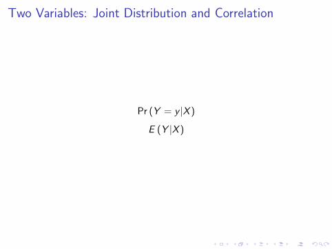
Two Variables: Joint Distribution and Correlation

Pr (Y = y |X )

E (Y |X )

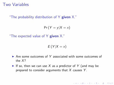
Two Variables

“The probability distribution of Y given X.”

Pr (Y = y |X = x)

“The expected value of Y given X.”

E (Y |X = x)

I Are some outcomes of Y associated with some outcomes ofthe X?

I If so, then we can use X as a predictor of Y (and may beprepared to consider arguments that X causes Y .

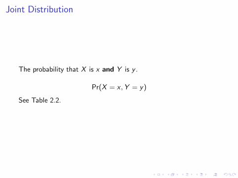
Joint Distribution

The probability that X is x and Y is y .

Pr(X = x ,Y = y)

See Table 2.2.

Marginal and Conditional Distributions

Marginal Distribution

The probability distribution of Y , ignoring X .

Conditional DistributionsThe probability distribution of Y given, or conditional on, X.

Pr (Y = y |X = x)

Review joint, marginal, and conditional distributions with

Table 2.3

Half, or 0.50, of all of the time we get an old computer (A = 0).Thirty-five percent, or 0.35, of all of the time we have an oldcomputer and experience no crashes (A = 0 and M = 0). Of the0.50 of all of the time that we get an old computer, 0.35 of all ofthe time we have no crashes. This means that conditional onhaving an old computer, we experience no crashes

0.35

0.50= 0.70

of the times that we have an old computer.

Bayes Law

Start with the intuitive (say this in words):What is the probability that X = x and Y = y are both true?It’s the probability that Y = y is true given that X = x is truetimes the probability that X = x is true.

Pr (X = x ,Y = y) = Pr (Y = y |X = x) Pr (X = x)

Reorganize into Bayes Law:

Pr (Y = y |X = x) =Pr (X = x ,Y = y)

Pr (X = x)

Bayes Law: Alternative

Note, by the way, that an alternative decomposition was possible:

Pr (X = x ,Y = y) = Pr (X = x |Y = y) Pr (Y = y)

Reorganize into Bayes Law:

Pr (X = x |Y = y) =Pr (X = x ,Y = y)

Pr (Y = y)

Bayes Law: Final form and interpretation

Pr (Y = y |X = x) =Pr (X = x ,Y = y)

Pr (X = x)

=Pr (X = x |Y = y) Pr (Y = y)

Pr (X = x)

=Pr (X = x |Y = y) Pr (Y = y)

Pr (X = x |Y = y) + Pr (X = x |Y 6= y)

Posterior probability depends on the prior and the evidence.

Bayes Law: Example

Surprising result from false positives on a test for a rare disease

Suppose Y is a Bernoulli random variable for having a rare disease.Pr (Y = 1) = 0.01, i.e., one percent prevalence in the population.Suppose X is a Bernoulli random variable for testing positive forthe disease. The test can deliver both false positives and falsenegatives, but it is fairly accurate. Pr (X = 1|Y = 1) = 0.95 andPr (X = 0|Y = 0) = 0.93. Thus the false negative rate is 0.05 andthe false positive rate is 0.07.Is a positive test result very bad news?

Pr (Y = 1|X = 1) =Pr (X = 1|Y = 1) Pr (Y = 1)

Pr (X = 1)

=0.95 × 0.01

0.01 × 0.95 + 0.99 × 0.07= 0.12 (1)

Independence

Learning X does not improve our guess about Y .

Pr (Y = y |X = x) = Pr (Y = y)

I From Probability Distribution to Expected Value & Variance

I Key concept: repeat application of the definition of E ()

Exercise 2.3 applied to Table 2.2 (Rain and Commute)

Compute E (Y )The long-commute rate is the fraction of days that have longcommutes. Show that the long-commute rate is given by 1−E (Y ).Calculate E (Y |X = 1) and E (Y |X = 0).Calculate the long-commute rate for (i) non-rainy days and (ii)rainy days.A randomly selected day was a long commute. What is theprobability that it was a non-rainy day? a rainy day?Are weather and commute time independent? Explain.

Exercise 2.3 applied to Table 2.2 (Rain and Commute)

Compute E (Y )

E (Y ) = 0 × Pr(Y = 0) + 1 × Pr(Y = 1)

= 0 × 0.22 + 1 × 0.78 = 0.78

The long-commute rate is the fraction of days that have longcommutes. Show that the long-commute rate is given by 1−E (Y ).Create a long-commute random variable, W .

Let W ≡ 1 − Y

E (W ) = E (1 − Y ) = 1 − E (Y )

For discussion: why expected value, not probability?

Calculate E (Y |X = 1) and E (Y |X = 0).

E (Y |X = 1) = 0 × Pr(Y = 0|X = 1) + 1 × Pr(Y = 1|X = 1)

Pr(Y = 0|X = 1) =Pr(Y = 0,X = 1)

Pr(X = 1)=

0.07

0.70= 0.1

Pr(Y = 1|X = 1) =Pr(Y = 1,X = 1)

Pr(X = 1)=

0.63

0.70= 0.9

E (Y |X = 1) = 0 × 0.1 + 1 × 0.9 = 0.9

What does this mean in words?

E (Y |X = 0) = 0 × Pr(Y = 0|X = 0) + 1 × Pr(Y = 1|X = 0)

Pr(Y = 0|X = 0) =Pr(Y = 0,X = 0)

Pr(X = 0)=

0.15

0.30= 0.5

Pr(Y = 1|X = 0) =Pr(Y = 1,X = 0)

Pr(X = 0)=

0.15

0.30= 0.5

E (Y |X = 0) = 0 × 0.5 + 1 × 0.5 = 0.5

What does this mean in words?Calculate the long-commute rate for (i) non-rainy days and (ii)rainy days.(i) What is the term that we want to compute?

E (W |X = 1) = 1 − E (Y |X = 1) = 0.1

(ii) What is the term that we want to compute?

E (W |X = 0) = 1 − E (Y |X = 0) = 0.5

A randomly selected day was a long commute. What is theprobability that it was a non-rainy day? a rainy day?What is the term that we want to compute?

Pr(X = 1|Y = 0) =Pr(X = 1,Y = 0)

Pr(Y = 0)

=0.07

0.22≈ 0.32

What is the term that we want to compute?

Pr(X = 0|Y = 0) =Pr(X = 0,Y = 0)

Pr(Y = 0)

=0.15

0.22≈ 0.68

Are weather and commute time independent? Explain.

Covariance

Covariance is another mean: The expected value of the product ofthe deviation of Y from its mean and the deviation of X from itsmean.

cov(X ,Y ) =

k∑

i=1

l∑

j=1

(xj − µX )(yi − µY ) Pr(X = xj ,Y = yi)

Observations

I This is another adding-up (∑

) over all the possible outcomesweighted by the likelihood of each outcome

I Focus on the key term:

(xj − µX )(yi − µY )

Interpreting covariance

(xj − µX )(yi − µY )

Are cases where X is above its mean usually paired with caseswhere Y is above its mean? (If so, then it will also be true thatcases where X is below its mean will usually be paired with caseswhere Y is below its mean.)In this case, the key term will be positive because⊕ times ⊕ is positive and times is positive.Are cases where X is above its mean usually paired with caseswhere Y is below its mean? (If so, then it will also be true thatcases where X is below its mean will usually be paired with caseswhere Y is above its mean.)In this case, the key term will be negative because⊕ times is negative and times ⊕ is negative.

Summary of covariance: Very Important

Positive covariance means that X and Y are typically big togetheror small together.Negative covariance means that when X is big, Y is small (andvice versa).

Units and Correlation

Covariance has awkward units (units of X × units of Y ). Aconvenient division gives a unitless measure that is bounded

between −1 and +1:

corr(X ,Y ) =cov(X ,Y )

s.d.(X ) × s.d.(Y )

(Recall that s.d.(X ) is measured in units of X and s.d.(Y ) ismeasured in units of Y .)Correlation near +1 means that X and Y are typically big togetheror small together.Correlation near −1 means that when X is big, Y is small (andvice versa).

Mean and Variance of Sums of R.V.’sSee Key Concept 2.3

Suppose that in a sample of couples X is income earned by the firstpartner and Y is income earned by the other partner. Householdincome is defined as the sum of these incomes, or X + Y .The mean value of household income is the sum of the mean valueof the first person’s earnings and the mean value of the secondperson’s earnings:

E (X + Y ) = E (X ) + E (Y ) = µX + µY

Mean and Variance of Sums of R.V.’s: Example

The variance of household income, an interesting measure ofinter-household inequality, is more complicated:

var (X + Y ) = var(X ) + var(Y ) + 2cov(X ,Y )

= σ2

X + σ2

Y + 2σXY

The spread of household income depends on the spread of incomefor each of the earners and whether high earners are paired withhigh earners or high earners are paired with low earners.(Can you think of economic or sociological reasons to expectcov(X ,Y ) to be positive or negative? What about change overtime?)