Availability and costs of liquefied bio- and synthetic methane
100
Availability and costs of liquefied bio- and synthetic methane The maritime shipping perspective
Transcript of Availability and costs of liquefied bio- and synthetic methane

Availability and costs of liquefied bio- and synthetic methane The maritime shipping perspective

1 190236 - Availability and costs of liquefied bio- and synthetic methane – March 2020
Availability and costs of liquefied bio- and synthetic methane The maritime shipping perspective
This report was prepared by:
Dagmar Nelissen, Japer Faber, Reinier van der Veen, Anouk van Grinsven, Hary Shanthi, Emiel van den Toorn
Delft, CE Delft, march 2020
Publication code: 20.190236.031
Maritime Shipping / Biofuels / Methane / Hydrogen / Availability / Production / Costs / Analysis / Technology /
Regulation
Client: SEA\LNG LTD
Publications of CE Delft are available from www.cedelft.eu
Further information on this study can be obtained from the contact person Dagmar Nelissen (CE Delft)
© copyright, CE Delft, Delft
CE Delft
Committed to the Environment
Through its independent research and consultancy work CE Delft is helping build a sustainable world. In the
fields of energy, transport and resources our expertise is leading-edge. With our wealth of know-how on
technologies, policies and economic issues we support government agencies, NGOs and industries in pursuit of
structural change. For 40 years now, the skills and enthusiasm of CE Delft’s staff have been devoted to
achieving this mission.

2 190236 - Availability and costs of liquefied bio- and synthetic methane – March 2020
Content
Acronyms 4
Executive Summary 5
1 Introduction 11 1.1 Background 11 1.2 Objective of study 12 1.3 Scope of study 12 1.4 Approach 14 1.5 Structure of report 15
2 Availability and cost price of liquefied biomethane (LBM) 16 2.1 Scoping analysis 16 2.2 Availability analysis 20 2.3 Cost analysis 35
3 Availability and cost price of liquefied synthetic methane (LSM) 42 3.1 Scoping analysis 42 3.2 Availability analysis 43 3.3 Cost analysis 55
4 Comparison of costs 61 4.1 Introduction 61 4.2 Production costs of synthetic and biomethane 61 4.3 Production costs of hydrogen 61 4.4 Production costs of ammonia 62 4.5 Liquefaction, transport and bunker infrastructure costs of the alternative fuels 63 4.6 Fossil bunker fuels 67 4.7 Cost comparison 69
5 Discussion of availability for and demand of shipping sector 72
6 Recommendations on how barriers to scaling of LBM and LSM as marine fuel could be
addressed 76 6.1 Barriers and conducive factors 76 6.2 Measures in the shipping sector 76 6.3 Measures in other sectors 77
7 Conclusions 78 7.1 Availability of LBM and LSM 78 7.2 Cost comparison 80 7.3 Recommendations for scaling up the use of LBM and LSM 80
3 190236 - Availability and costs of liquefied bio- and synthetic methane – March 2020
8 Literature 82
A GHG-accounting methods for biofuel 91 A.1 Intergovernmental Panel on Climate Change (IPCC) 91 A.2 Renewable Energy Directive and Fuel Quality Directive 91
B Production capacity of electrolysers 93 B.1 Technology maturity and characteristics 93
C Levelized costs of renewable electricity 95
D Production cost estimations 96 D.1 Ammonia 96 D.2 Hydrogen 98

4 190236 - Availability and costs of liquefied bio- and synthetic methane – March 2020
Acronyms
Abbreviation
AD Anaerobic Digestion
AEC Alkaline Electrolysis Cell
AHPD Autogenerative High Pressure Digestion
CAPEX Capital Expenditure
DAC Direct air capture
EJ Exajoule
FLH Full load hours
FQD Fuel Quality Directive (2009/30/EC)
GHG Greenhouse Gas(es)
HFO Heavy fuel oil
HGV Heavy goods vehicle
HSH Hot standby hours
ILUC Indirect Land Use Change
km Kilometre
kW Kilowatt
kWe Kilowatt-electric
kWth Kilowatt-thermal
kWh Kilowatt hour
LBM Liquefied biomethane
LNG Liquefied natural gas
LSM Liquefied synthetic methane
MEPC Marine Environment Protection Committee
MEUR Million Euro
MGO Marine Gas Oil
MMBtu million British thermal units
mt Metric ton
Mt Megaton
MW Megawatt
MWe Megawatt-electric
MWth Megawatt-thermal
MWh Megawatt hour
NG Natural gas
OPEX Operational Expenditures
PEM Proton Exchange Membrane
PtG Power to Gas
RED Renewable Energie Directive (2009/28/EC)
RED II Revised Renewable Energy Directive (2018/2001/EU)
SOEC Solid Oxide Electrolyser Cell
TPH Thermal Pressure Hydrolysis (TPH)
TRL Technology Readiness Level
TWh Terawatt hour
VLSFO Very low sulphur foil oil

5 190236 - Availability and costs of liquefied bio- and synthetic methane – March 2020
Executive Summary
Currently, a small, but growing number of ships are LNG-fuelled. This is mainly due to
stricter air pollution regulation for maritime shipping. Decarbonisation of the maritime
shipping sector requires the use of zero/low carbon fuels and the use of liquefied
biomethane (LBM) or liquefied synthetic methane (LSM) is a potential decarbonisation
pathway for shipping. LNG-fuelled ships could then use LBM or LSM without major
modifications and a technically mature LNG infrastructure would only need to be scaled up.
The volumes of LBM and LSM that will become available to the shipping industry and the
relative costs of these fuels compared to other zero/low carbon fuels are crucial for the
viability of this pathway.
Against this background, this study aims:
— to assess the global availability of LBM and LSM in relation to the global energy demand
of maritime shipping;
— to assess the cost price of LBM and LSM and to compare it with the cost (price) of other
existing and potential marine bunker fuels; and
— to make recommendations as to how industry and policy makers could address barriers
to the scaling of LBM and LSM as a marine fuel.
The study focuses on 2030 and 2050, years in which important milestones in the IMO Initial
Strategy on Reduction of GHG Emissions will have to be met.
The study is based on review of scientific and grey i.e. non-academic literature.
Availability of biomethane
Biomethane can be made from different types of biomass and by means of different
conversion technologies. Conducting a literature review, this study has analysed the
maximum conceivable sustainable supply of the following biomass streams:
— energy crops (grown solely for energy purposes);
— agricultural residues;
— forestry products and residues; and
— aquatic biomass.
The maximum conceivable sustainable supply is defined as the maximum supply that can be
produced in a sustainable way. Different literature sources apply different definitions of
sustainability. Most have in common that they rule out biomass streams, interfering with
the growth of food, fodder and fibres.
Taking into account the efficiency of the different production routes and of liquefaction,
Figure 1 compares the maximum conceivable sustainable supply of LBM with the projected
energy demand from the maritime sector in 2030 and 2050. The maximum conceivable
sustainable biomethane potential is expected to range from roughly 40 to 120 EJ in 2030
and from roughly 40 to 180 EJ in 2050, compared with projected energy demand from
shipping of 12-14 EJ in 2030 and 10-23 EJ in 2050. In addition to the biomass streams
depicted in Figure 1, aquatic biomass has the potential to play a dominant role, especially
in 2050 (550–1,300 EJ biomethane). However, only a few studies have looked into the global
availability of aquatic biomass so far and it is not possible to draw firm conclusions on its
maximum sustainable supply.
6 190236 - Availability and costs of liquefied bio- and synthetic methane – March 2020
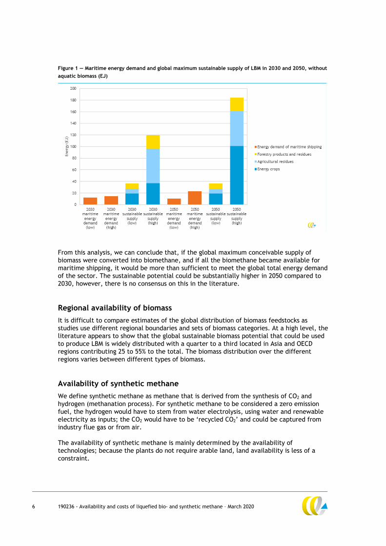
Figure 1 — Maritime energy demand and global maximum sustainable supply of LBM in 2030 and 2050, without
aquatic biomass (EJ)
From this analysis, we can conclude that, if the global maximum conceivable supply of
biomass were converted into biomethane, and if all the biomethane became available for
maritime shipping, it would be more than sufficient to meet the global total energy demand
of the sector. The sustainable potential could be substantially higher in 2050 compared to
2030, however, there is no consensus on this in the literature.
Regional availability of biomass
It is difficult to compare estimates of the global distribution of biomass feedstocks as
studies use different regional boundaries and sets of biomass categories. At a high level, the
literature appears to show that the global sustainable biomass potential that could be used
to produce LBM is widely distributed with a quarter to a third located in Asia and OECD
regions contributing 25 to 55% to the total. The biomass distribution over the different
regions varies between different types of biomass.
Availability of synthetic methane
We define synthetic methane as methane that is derived from the synthesis of CO2 and
hydrogen (methanation process). For synthetic methane to be considered a zero emission
fuel, the hydrogen would have to stem from water electrolysis, using water and renewable
electricity as inputs; the CO2 would have to be ‘recycled CO2’ and could be captured from
industry flue gas or from air.
The availability of synthetic methane is mainly determined by the availability of
technologies; because the plants do not require arable land, land availability is less of a
constraint.

7 190236 - Availability and costs of liquefied bio- and synthetic methane – March 2020
Water electrolysis and methanation are well-established processes. Carbon capture at the
stack of an industrial plant is also a well-established process. In the long-run, direct air
capture (DAC) and carbon capture at the stack of bioenergy production plants are more
relevant options. Renewable electricity technologies are mature, with the efficiency of
some technologies expected to further increase in the future. Hence, all technological
processes that are required to produce synthetic methane can be considered to be mature
or near maturity.
Figure 2 shows the energy demand from maritime transport and the amount of renewable
electricity that would be required to meet this demand with LSM. Because of projected
improvements in the production process, the renewable electricity demand will decrease
when the projected energy demand increases. The amount of renewable electricity
required to produce LSM for the maritime sector is compared with the projected amount of
renewable electricity that will be required to limit global warming to 2 degrees above pre-
industrial levels. In 2050, an estimated 25-30% of renewable electricity would need to be
produced in addition to the projected amount to decarbonise the maritime transport sector
using LSM.
Figure 2 — Maximum potential supply of LSM compared with maritime energy demand given a renewable
electricity supply in line with a 2°C degree scenario
From this analysis we can conclude that the current global share of renewable electricity is
insufficient to produce sufficient LSM to power a significant share of the fleet. The situation
is projected to improve, although the investments require adequate policies. And it remains
to be seen how much of the renewable electricity will be available for the production of
hydrogen which is a necessary feedstock for all synthetic fuels such as LSM, green hydrogen
and ammonia.
0
20
40
60
80
100
120
140
160
180
2015 2030 2050
EJ
Maritime energy demand
Required renewable electricity to power maritime shipping with LSM using available productiontechnologies
Available renewable electricity (2°C scenarios)
8 190236 - Availability and costs of liquefied bio- and synthetic methane – March 2020
Discussion of availability for and demand of shipping sector
The analysis of the availability of LBM has focused on the global maximum conceivable
supply and the analysis of the availability of LSM on the renewable electricity required to
supply the entire shipping sector with LSM.
It would however be unrealistic to assume that these volumes of LBM/LSM would all become
available to the shipping sector: Biomass that can be used for the production of LBM could
be utilised in alternative ways, i.e. either used directly or for production of other gaseous
or liquid biofuels and hydrogen. And the renewable electricity used for the production of
LSM could also be used differently, i.e. either used directly or for the production of other
synthetic gaseous or liquid fuels.
Currently, most natural gas is used in the power sector, industry and the built environment.
It can be expected that the power sector and industry will reduce their demand for
methane when the economy moves away from fossil fuels. The built environment, land-
based, HGV transport and shipping may see a continued or an increased demand for
methane from renewable sources.
In order to scale up the use of LSM and LBM in the shipping sector, it could be relevant to
reduce the uncertainty about the use of methane as a fuel, especially with regards to
methane slip and the associated climate impact. Policy measures like a fossil carbon levy,
emissions trading or a low-carbon fuel standard could be implemented to shift the demand
in the shipping sector from natural gas or liquid fossil fuels to LSM, LBM or other low- and
zero-carbon fuels.
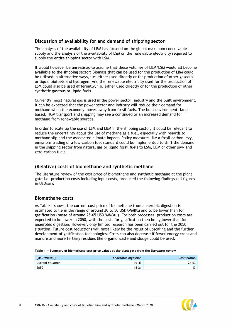
(Relative) costs of biomethane and synthetic methane
The literature review of the cost price of biomethane and synthetic methane at the plant
gate i.e. production costs including input costs, produced the following findings (all figures
in USD2019):
Biomethane costs
As Table 1 shows, the current cost price of biomethane from anaerobic digestion is
estimated to lie in the range of around 20 to 50 USD/MMBtu and to be lower than for
gasification (range of around 25-65 USD/MMBtu). For both processes, production costs are
expected to be lower in 2050, with the costs for gasification then being lower than for
anaerobic digestion. However, only limited research has been carried out for the 2050
situation. Future cost reductions will most likely be the result of upscaling and the further
development of gasification technologies. Costs can also decrease if fewer energy crops and
manure and more tertiary residues like organic waste and sludge could be used.
Table 1 — Summary of biomethane cost price values at the plant gate from the literature review
[USD/MMBtu] Anaerobic digestion Gasification
Current situation 19-49 24-63
2050 15-21 13

9 190236 - Availability and costs of liquefied bio- and synthetic methane – March 2020
Synthetic methane costs
The estimations of the cost price of synthetic methane vary significantly: for 2030 around
23-110 USD/MMBtu and for 2050 around 15-60 USD/MMBtu. Different assumptions regarding
the price of renewable electricity and the load of the electrolyser are the main reasons for
this large range. Renewable electricity prices play a major role for the cost price of
synthetic methane. These factors also hold for the production of green hydrogen and other
synthetic fuels such as ammonia.
Cost comparisons with alternative bunker fuels
Two comparisons between the costs of alternative bunker fuels have been conducted in the
study. Since data availability for 2050 is rather poor, these comparisons focus on 2030.
First, the expected bunker fuel prices of fossil fuels (VLSFO, fossil LNG) and the expected
cost price of two post-fossil fuels (LSM, LBM) at point of delivery in port have been
compared. Regarding the fossil bunker fuels, a carbon mark-up has been accounted for,
assuming that an according climate policy measure will be in force in 2030.
This first cost comparison shows:
— Per energy unit, fossil LNG would be the cheapest and LSM the most expensive bunker
fuel in 2030. Fossil LNG is estimated to be between 1 to 11 USD/MMBtu cheaper than
VLSFO. LSM can only be cheaper than LBM, if cheap renewable electricity is available
and high electrolyser load factors can be achieved.
— A carbon mark-up of between 50–100 USD/t CO2, the 2030 carbon price level that is
considered consistent with achieving the Paris temperature target, will not be sufficient
to incentivize a switch from fossil LNG to LBM or LSM in 2030. However, a 2050 carbon
price that is consistent with a well below 2°C mitigation pathway i.e. between 300 and
400 USD/t CO2, can be expected to incentivize a switch from fossil LNG to LBM, at least
if the 2050 price for fossil LNG is not below its 2030 price.
Second, the cost price of different alternative, renewable fuels (liquid hydrogen, liquid
ammonia, LSM, LBM) are compared at the plant gate (see Table 2) i.e. before any costs
associated with transport, distribution and bunkering, which are still uncertain for hydrogen
and ammonia, are taken into account.
Table 2 — 2030 plant gate cost price estimates for different renewable bunker fuels
Cost price at plant gate (USD/MMBtu)
LBM 21-48
LSM 26-113
Liquid ammonia 17-105
Liquid hydrogen 19-72
From this second cost comparison we can conclude the following:
— In an optimistic scenario (lower range of the cost estimates from the literature review),
• plant gate costs are broadly comparable for LBM, liquid ammonia and liquid
hydrogen;
• plant gate costs of liquid ammonia are expected to be lowest, followed by liquid
hydrogen and LBM with LSM featuring the highest costs. Significantly lower
liquefaction costs for ammonia can explain the cost differential between liquid

10 190236 - Availability and costs of liquefied bio- and synthetic methane – March 2020
ammonia and liquid hydrogen, but the presumed optimistic electricity price might
also vary between the estimates.
— In a pessimistic scenario (higher range of cost estimates from the literature review),
plant gate costs are expected to be lowest for LBM, followed by liquid hydrogen; costs
for both, liquid ammonia and LSM are relatively high and highest for LSM.
The optimistic scenario will probably only materialise for liquid hydrogen, liquid ammonia
and LSM if the production location has favourable conditions for renewable electricity.
This may require the transportation of the produced fuels over longer distances, depending
on the locations of the bunker ports.
If transported by ship, transportation costs can be expected to be lower for liquid ammonia
compared to liquid hydrogen and LSM and indeed, LBM: due to ammonia’s relatively high
boiling point it can become liquid at relative low pressure and/or under relatively mild
conditions. Liquefaction, storage and transport costs are therefore lower than for hydrogen
and LSM/LBM; for liquid hydrogen these costs are can be expected to be higher than for
LSM/LBM.
Since the production of LBM does not rely on the availability of cheap renewable electricity,
this might allow for local production in the vicinity of major ports and could save out costs
for the transport of the bunker fuel. Local production of LBM might however require
transport of biomass. These transport costs can be expected to be relatively low, at least if
the biomass can be transported/is available in bulk.
As the costs of the bunker infrastructure for hydrogen and ammonia are not known, their
impact on the bunker fuel prices are difficult to assess at present. However, given that the
bunkering infrastructure for LBM and LSM are technically mature and commercially available
whereas the bunkering infrastructure for hydrogen and ammonia is technically still
immature, the bunker price cost mark-up for the bunkering of hydrogen and ammonia can
be expected to be higher than for LSM and LBM, at least in the short- and medium-run.
Conclusions
The future maximum conceivable sustainable supply of LBM and LSM exceeds the energy
demand from the shipping sector, provided that biomass will be used to produce methane
and sufficient investments are made in renewable electricity production. The production
costs of these fuels need not be significantly higher and could be comparable to the
production costs of other low- and zero-carbon fuels. So, if the costs of bunkering
infrastructure and ships are comparable as well, LSM and LBM would be viable candidate
fuels for a decarbonised shipping sector.
11 190236 - Availability and costs of liquefied bio- and synthetic methane – March 2020
1 Introduction
1.1 Background
The current air quality requirements for ships in Emission Control Areas and the upcoming
global cap on the sulphur content of fuel oil of 0.50% m/m provide an incentive to use
liquefied natural gas (LNG) as marine bunker fuel. In consequence, the number of
LNG-fuelled and LNG-ready ships1 is currently2 rising: according to Clarksons Research,
around 525 LNG-capable ships are in the fleet and around 330 on order.
The Initial IMO Strategy on Reduction of GHG Emissions from Ships (Resolution
MEPC.304(72)) aims to phase-out greenhouse gas emissions from international shipping as
soon as possible in this century. In addition, the Strategy sets the ambitions to:
— improve the carbon intensity of shipping by at least 40% in 2030, relative to 2008 and
pursue efforts to improve it by 70% by 2050; and
— reduce the greenhouse gas emissions of shipping by at least 50% in 2050, relative to
2008.
The Initial Strategy also notes that ‘the global introduction of alternative fuels and/or
energy sources for international shipping will be integral to achieve the overall ambition’.
It is generally understood that these fuels and energy sources will contain significantly
less/no fossil carbon compared to the bunker fuels currently used.
Given the IMO’s Initial GHG Reduction Strategy, the question arises for how long
LNG-fuelled ships and LNG bunker fuel infrastructure will be viable.
Whether an investment in an LNG-ready ship is profitable thereby depends on the total cost
of ownership of the different possible combinations of propulsion systems and bunker fuels
a ship owner has at hand, given the air quality regulations for maritime shipping and given
that at a later point in time the ships might — depending on their life time — have to switch
to renewable bunker fuel, either as a drop-in fuel or as a fuel that would require additional
retrofits.
Liquefied bio- and synthetic methane3 (LBM and LSM) could play an important role in this
context since it could substitute fossil marine LNG4. The future availability of LBM and LSM
as well as the cost prices of these fuels are therefore the focus of this study.
________________________________ 1 LNG-ready ships can relatively easily be converted to LNG-capable ships. 2 September 2019. 3 Focus of the study are two types of low/zero carbon bunker fuels that can easily substitute the current marine
LNG which we call ‘liquefied bio-methane’ and ‘liquefied synthetic methane’. We decided not to work with the
terms ‘bio LNG’ and ‘synthetic LNG’ to avoid the association with fossil natural gas. 4 LNG is typically composed of methane, ethane, propane and nitrogen, with the composition depending on the
origin of the natural gas. Main component is always methane with its share ranging from 80-99% (IGU, 2012).
Using methane instead of LNG might require retrofits which we however expect to be minor.

12 190236 - Availability and costs of liquefied bio- and synthetic methane – March 2020
1.2 Objective of study
The aim of the study is threefold:
1. To assess the availability of LBM and LSM in relation to the global energy demand of
maritime shipping.
2. To assess the cost price of LBM and LSM and to compare it with the cost (price) of other
existing and potential marine bunker fuels.
3. To give recommendations as to how industry and policy makers could address barriers to
the scaling of LBM and LSM as a marine fuel.
1.3 Scope of study
The scope of the specific tasks are discussed in the according sections of the report; the
general scope of the study is as follows:
Time horizon
We assume that the fleet will be required to, and will, meet the IMO targets as specified in
the Initial IMO Strategy on Reduction of GHG Emissions from Ships. Specifically, we assume
that the following targets will be met:
— by 2030 the fleet’s carbon intensity is reduced by at least 40% relative to 2008;
— by 2050 the fleet’s carbon intensity is reduced by at least 70% and the total annual
GHG emissions by at least 50% relative to 2008;
— as soon as possible after 2050 the fleet is fully decarbonized.
Given these targets, this study will focus on cost and availability scenarios for 2030 and
2050.
Alternative bunker fuels
The scope of the availability analysis is limited to LBM and LSM. The availability of other
low-/zero-carbon bunker fuels, such as hydrogen, synthetic ammonia, methanol or biodiesel
is not analysed.
Geographic scope
The study assesses the availability of LBM and LSM on a global level and relate them to the
global energy demand of the global fleet engaged in international shipping.
Assessment of availability
This study assesses the maximum conceivable supply of LBM. This means that when
assessing the availability of LBM we assume that the available volume of a relevant biomass
feedstock will entirely be used to produce LBM, at least if the production capacity allows
for this. In other words, the study does not take competition for resources into account.
In addition, the study does not estimate the share of the maximum conceivable supply that
might become available for the shipping sector. In Chapter 5 however, the availability for
and the demand of LBM/LSM for the shipping sector is discussed.

13 190236 - Availability and costs of liquefied bio- and synthetic methane – March 2020
Although the maximum conceivable supply implies an assessment of the technical potential
only, this is not possible in practice. In reality, the technical and economic potential are
strongly intertwined: especially the technical potential is determined by many economic
factors. The business case of alternative fuels is heavily influenced by policy incentives and
technological developments are also influenced by policy objectives and economic
incentives, such as subsidies or obligations. In this report, we define the maximum
conceivable supply as the supply that could be achieved assuming that investments in LBM
and LSM are profitable, either through market factors or through regulatory intervention.
Shipping sector
The study focuses on the shipping sector, noting that other sectors may compete for
biomethane, synthetic methane, biomass, renewable electricity and other inputs to the
production of biomethane and synthetic methane.
Assessment of costs
To be able to assess the affordability of LBM and LSM for the shipping sector, production
costs of LBM and LSM are estimated for 2030 up until the point of delivery to a ship.
They are compared with bunker price estimates of fossil LNG and VLSFO, taking a carbon
mark-up into account.
In addition, the estimated 2030 cost price at plant of LBM and LSM is compared with the
cost price at plant of two alternative, renewable fuels (liquid hydrogen and ammonia).
Transport and bunker infrastructure costs are not considered in this context.
When comparing the cost (price) of different bunker fuel types, the actual change of the
ships’ operational costs is not considered, i.e. the energy efficiency of the different
according propulsion systems is not accounted for.
Conversion routes hydrogen and other synthetic fuels considered
Next to fossil bunker fuels and LBM, the cost analysis considers hydrogen, LSM, and
ammonia. For the hydrogen as such and for the hydrogen that is required as an input for the
production of LSM and ammonia, the study considers so-called green hydrogen.
Green hydrogen is produced by means of water electrolysis.
Blue hydrogen is not considered in this study. If blue hydrogen, which is produced from
natural gas, would be used instead of green hydrogen, the CO2 stemming from the
combustion of the blue hydrogen and the synthetic fuels based on blue hydrogen would
have to be captured and stored for the fuels to be considered low/zero fossil carbon fuels.
CO2 storage capacity will be scarce in the long run and could therefore restrict the volume
of blue hydrogen/fuels based on blue hydrogen to be used. In addition, blue hydrogen in
combination with CCS is, at least in the long run, expected to be more expensive than green
hydrogen.5
________________________________ 5 See for example (Lloyd's Register; UMAS, 2019) and (CE Delft, 2018b).

14 190236 - Availability and costs of liquefied bio- and synthetic methane – March 2020
GHG reduction potential
In the value chain of marine fuels two main phases can be distinguished: well-to-hull and
hull-to-wake.
In the well-to-hull phase of fossil marine LNG, natural gas is extracted, processed,
transported to and stored at a main LNG terminal and is subsequently distributed to ports
for bunkering. In this first phase, GHG emissions result from the combustion of different
fossil fuels and from uncombusted natural gas which can slip at different points in the value
chain as well as due to flaring and venting practices during natural gas production.
Flaring6 and venting are applied if the gas quality is not sufficient or if there is not
sufficient pipeline capacity. In the hull-to-wake phase, LNG is used on board ships, with
GHG emissions resulting from the combustion of LNG and from the slip of uncombusted
methane. The amount of methane slip thereby depends on the engine type and the
operation of the engines.
If LBM or LSM is used instead of LNG, the hull-to-wake carbon emissions should be
accounted for as zero emissions (see Annex A for an overview of how the GHG emissions of
biofuels are accounted for under IPCC and EU rules), whereas the other hull-to-wake GHG
emissions can be expected to be the same as for fossil LNG and should be accounted for in
the same way.
The well-to-hull emissions of LBM and LSM can expected to change compared to fossil LNG,
due to structurally different supply chains.
The actual GHG reduction potential of LBM and LSM and the other alternative fuels are out
of the scope of the study.
1.4 Approach
Figure 3 shows a schematic overview of the supply chain of LBM and LSM, with on the left a
list of criteria applied to estimate the maximum conceivable supply. For both fuel types,
we thereby start off with a scoping analysis in which the different possible production
processes and inputs are described and relevant combinations of production process and
inputs are elaborated. The next step includes an assessment of feedstock availability and
feedstock cost. In the following step, the conversion technologies are assessed using
criteria, such as technology readiness level (TRL)7, etc. Lead times to increase production
capacity are especially relevant in relation to 2030.
________________________________ 6 Flaring leads to methane emissions if not properly operated. 7 Technology readiness levels indicate how close to commercialisation technologies are. 9 levels are
differentiated: Level 1 indicates the lowest and Level 2 the highest readiness.

15 190236 - Availability and costs of liquefied bio- and synthetic methane – March 2020
Figure 3 — Schematic overview of supply chain of LBM and LSM
1.5 Structure of report
The study is structured as follows:
— Chapters 2 and 3 analyse the availability and the cost price of LBM and LSM
respectively.
— Chapter 4 compares the expected cost price of LBM and LSM with the expected (cost)
price of other marine bunker fuels.
— Chapter 5 discusses the availability of and demand for LBM and LSM by the maritime
shipping sector.
— Chapter 6 gives recommendations to industry and policy makers as to how to address
practical barriers to the scaling of LBM and LSM as marine fuel.
— Chapter 7 presents the main conclusions from the study.
16 190236 - Availability and costs of liquefied bio- and synthetic methane – March 2020
2 Availability and cost price of
liquefied biomethane (LBM)
In this section we estimate the maximum global availability (Section 2.2) and cost price
(Section 2.3) of methane that is produced from biomass feedstocks in the current situation,
as well as in 2030 and 2050. In order to determine the global availability of LBM, we first
identify the main conversion routes and biomass feedstocks (Section 2.1). The analyses have
been carried out by means of a literature review.
2.1 Scoping analysis
In the scoping analysis we identify and describe the main conversion routes and biomass
feedstocks for the production of biomethane and present relevant technology-feedstock
combinations.
2.1.1 Main conversion routes
As depicted in Figure 4, there are two main types of conversion routes for the production of
biomethane from biomass: anaerobic digestion and gasification.
Anaerobic digestion is a collection of processes in which microorganisms break down
biomass feedstocks in the absence of oxygen. The feedstocks sometimes undergo a
pre-treatment step such increasing the moisture content to the required level.
The anaerobic digestion processes result in biogas, which is a mixture of methane, carbon
dioxide (30-50%), and other gasses such as hydrogen sulphide. In an upgrading step, the
carbon dioxide is separated from the (bio)methane.
Gasification is a process in which biomass feedstocks react at high temperatures (> 700°C)
with a certain amount of oxygen and/or steam and are converted into syngas (short for
synthesis gas), which is a gas mixture that consists mainly of hydrogen and carbon
monoxide. In a preceding pre-treatment step biomass is dried and reformed by means of
pyrolysis (Sikarwar, et al., 2016). After gasification, gas cleaning and conditioning, the
syngas is fed into a methanation process.
Independent of the conversion route, biomethane has to be liquefied to obtain LBM.

17 190236 - Availability and costs of liquefied bio- and synthetic methane – March 2020
Figure 4 — The two main conversion routes for the production of LBM
Various detailed technology options fall under these two main conversion routes. These deal
particularly with the core system (the AD system or the gasifier) and are listed below.
Note that not all of the technologies are technologically mature at present, but as shown
further down in the report, all of the following technologies can be expected to become
technologically mature in the coming decades.
For the anaerobic digestion conversion route, technology options are:
— Single-stage: “all wastes are loaded simultaneously, and all AD processes are allowed to
occur in the same reactor” (Meegoda, et al., 2018).
— Multi-stage: digestion steps in different reactors.
— Mono-, co-, and all-feedstock digesters: Digestion units can be designed and optimized
for a specific single feedstock types or for multiple feedstocks. However, the used
process technology is essentially the same. The different types of digesters are further
considered below, as used feedstock types and unit sizes do differ. Manure digestion is a
common type of mono-digestion (CE Delft, 2018c).
— Autogenerative High Pressure Digestion (AHPD): This is an innovative technology
developed and patented by the Dutch company Bareau. It produces relatively pure
biomethane without biogas as an intermediate product. Thus, the upgrading step is not
part of the conversion route of this technology (CE Delft, 2018c).
— Thermal Pressure Hydrolysis (TPH): Feedstocks are, together with process water,
heated to 150-160°C and pressurized, resulting in partial hydrolysis of the biomass.
By means of instantaneous pressure release the water evaporates in such a way that the
molecule structure of the biomass is cracked (CE Delft, 2018c).
For gasification, the technology options are:
— Wood gasification:
Fixed bed: Has a simple configuration and is flexible in use of feedstocks. Capacity
of 1-10 MWth. (WBA, 2015);
Fluidized bed: Capacity of 10-200 MWth (WBA, 2015);
Entrained flow: High conversion efficiency but requires feedstock fractions smaller
than 1 mm. Unit capacities from 2 MWth to more than 100 MWth (WBA, 2015).
— Plasma gasification: Emerging technology. “Usage of plasma as a heat source during
gasification or as a tar-cracking agent downstream”. Has high investment cost, is
electricity intensive and has a low efficiency (Sikarwar, et al., 2016).
— Supercritical water gasification: Emerging technology. Form of hydrothermal
gasification. Gasification carried out in supercritical water. Liquid biomass and solid
biomass with a high moisture content can be processed with this (Singh Sikarwar et al.,
2016). Solid biomass can be used as well, but needs to be broken down in small particles

18 190236 - Availability and costs of liquefied bio- and synthetic methane – March 2020
and mixed with water to create a pumpable slurry in the pre-treatment step (Pinkard,
et al., 2019).
2.1.2 Biomass feedstocks
Essentially, all types of biomass feedstock could be used for the production of biomethane.
A classification of biomass feedstocks, differentiating between the type of stream and the
sector the stream stems from, are given in Table 3. Also, some examples of specific
feedstock types are provided.
Table 3 — Classification of biomass feedstocks
Sector Type of stream Examples of specific feedstock types
Agriculture Production Maize, sugarcane, sugar beet, soy, rapeseed
Primary residues Beet leaves, straw, solid manure, slurry (wet manure)
Secondary residues Beet pulp, slaughterhouse waste, shells
Tertiary residues Organic fraction of municipal solid waste, other organic waste,
sewage sludge, disposed textile, used fats and oils, landfill gas
Forestry Production Roundwood
Primary residues Branches, leaves, bark, roots
Secondary residues Sawdust, black liquor
Tertiary residues Waste wood, disposed paper and cardboard
Aquaculture Production Algae, sea weed
Secondary residues By-products from biodiesel production from aquatic biomass, waste
from fish-farming
Other Production Lignocellulosic energy crops (willow, poplar, miscanthus, switch
grass)
Primary residues Roadside grass, biomass from maintenance of reed beds and
watercourses, landscape care wood
In studies on global biomass potential, a distinction is often used between the following
four biomass categories:
1. Energy crops (grown solely for energy purposes).
2. Agricultural residues.
3. Forestry products and residues.
4. Aquatic biomass.
For this reason, we will adopt these four biomass categories in the availability analysis
presented in Section 2.2.
Based on sustainability assessments and frameworks foreseen for the future, such as the
EU Renewable Energy Directive (RED II), not all four categories of biomass are preferred to
be used to the same extent as renewable energy source. For energy crops for example, the
RED II caps the contribution from food and feed crops, which means that the use of these
feedstocks is limited due to sustainability concerns, especially in relation to indirect land
use change (ILUC). For biomethane from anaerobic digestion based on maize is therefore
less desirable from an RED II-perspective, because maize falls within the category of food
and feed crops. There is, however, an option to use food and feed crops in case their low-
ILUC risk can be proven by means of certification as laid down in the delegated act from
March 2019. Due to this possibility, it is hard to simply exclude this category of energy crops
in this analysis, but we will present energy crops as a separate category in the results.

19 190236 - Availability and costs of liquefied bio- and synthetic methane – March 2020
The use of used cooking oil and animal fats is capped under the RED II too. Their availability
is limited. This implies that the increase in renewable energy required to meet the EU
renewable energy target for transport has to come from advanced biofuels stemming from
other residues. Biofuels from aquatic biomass produced in installations on land are
classified as advanced biofuels, but biofuels produced from macroalgae (seaweed)
cultivated at sea are not, because the magnitude of the associated environmental risks are
still uncertain (see Section 2.2.3). Other options, including manure, organic waste and
agricultural residues will be classified as advanced biofuels and are favoured under the
RED II-framework. In addition, developments and growth in gasification will open up the
options to also include more forestry residues, which are also listed as potential feedstocks
for advanced biofuels.
Regarding the using of roundwood (biomass from forestry production), it must be noted that
the sustainability of this type of biomass is subject to debate. The sustainability is to a
large extent determined by how forests are being managed. However, many small forest
owners in North America have not certified their wood resources. This does not necessarily
mean that their wood resources are unsustainable but means the sustainability can at least
not be proven. Another point of discussion is carbon debt. Carbon debt can be defined as
the carbon balance of wood resources between reduced carbon stocks of a forest due to
harvesting or land-use on the one hand, and carbon sequestration through forest (re)growth
and carbon offsets of avoiding emissions from fossil fuels on the other (Hanssen, 2015).
In other words: carbon debt is about the difference between the pace of emitting CO2 from
wood combustion versus how fast a forest can recapture the CO2 again. Stakeholders do
have discussions on what payback time is required to restore the carbon balance in relation
to the GHG emission reduction targets of various sectors.
2.1.3 Technology-feedstock combinations
Different biomass conversion technologies exist, each with their own set of suitable biomass
feedstocks. Table 4 provides an overview of the different anaerobic digestion and
gasification technologies, along with their suitable feedstock types, typical unit sizes and
technology readiness levels.
Table 4 — Conversion routes, underlying technologies and corresponding characteristics (based on CE Delft,
2018c)
Conversion
route
Technology Feedstocks Unit size Technological readiness level
Anaerobic
digestion
Manure digestion Slurry (cow and pig),
solid manure (cow)
Often small scale
(20-50 m3 biogas per
hour)
Commercial
Co-digestion Manure, sludge, organic
waste, maize, straw,
roadside grass
Small to middle-large
scale
(~500 m3 biogas per hour)
Commercial
All-feedstock
digestion
Manure, sludge, organic
waste, maize, straw,
roadside grass
Large scale
(800-10,000 m3 biogas per
hour)
Commercial
Dry digestion Organic waste, maize Large scale
(~1,500 m3 biogas per
hour)
Commercial
Thermal Pressure
Hydrolysis (TPH)
Sludge Middle-large scale
(~350 m3 biogas per hour)
Commercial

20 190236 - Availability and costs of liquefied bio- and synthetic methane – March 2020
Conversion
route
Technology Feedstocks Unit size Technological readiness level
Autogenerative High
Pressure Digestion
(AHPD)
Sludge, manure (pig),
agricultural residues
Unknown TRL 8 (scale-up phase)
Gasification Wood gasification Woodchips (from forestry
production and primary
residue streams), bark,
waste wood
From 10 MW to
considerably larger
volumes
Demonstration units on semi-
commercial scale
Supercritical water
gasification
All types of biomass
feedstocks
0.7-3.3 MW a Pilot plant is under construction
in the Netherlands
Sources: a: STOWA (2016); If no source is indicated, the source is CE Delft (2018c).
Table 4 shows that different dedicated anaerobic digestion systems have been developed
for different biomass feedstock types. The unit sizes of digesters are often optimized based
on the types of feedstocks used and the available feedstock volumes (CE Delft, 2018c).
Gasification systems are generally not optimised for particular feedstocks, as the
gasification process is not as dependent on feedstock composition as is the AD process.
Gasification systems typically use dry, woody (lignocellulosic) biomass, whereas anaerobic
digestion systems use wet feedstock types. However, supercritical water gasifiers can
process all types of feedstocks, both woody and non-woody. These gasifiers require wet
feedstocks, which means that dry biomass must be mixed with water.
An important technical observation is that most anaerobic digestion technologies have
entered the market, whereas gasification technologies still need to be demonstrated
commercially.
2.2 Availability analysis
In this section we determine the maximum conceivable global supply of LBM in the current
situation, in 2030 and 2050. This amount poses a physical limit on the amount of LBM that
could possibly be used by marine shipping worldwide.
The maximum conceivable supply is calculated by taking into account three main factors:
— the global availability of relevant biomass feedstocks;
— the development of the global biomethane production capacity; and
— the LBM production yield of the conversion routes, assuming all biomethane will be
converted to LBM.
We will discuss these factors separately before calculating the maximum conceivable supply
of LBM.
2.2.1 Global availability of biomass feedstocks
Bioenergy provides around 9% of global primary energy demand, a high share of which is
‘traditional’ bioenergy in the form of charcoal from unsustainable deforestation, used in
developing countries to produce heat for cooking. Other forms of bioenergy add up to 4% of
global primary energy demand (CCC, 2018). Considering that the global primary energy
supply was 571 EJ in 2015 (IEA, 2017b), the current contribution of biomass to energy
consumption worldwide is about 50 EJ.

21 190236 - Availability and costs of liquefied bio- and synthetic methane – March 2020
When studying the bioenergy potential, it is important to distinguish between different
‘types’ of potentials. Bioenergy potential studies often estimate a technical potential
and/or a sustainable potential. The technical potential is the biomass that could become
available for the production of bioenergy. The use of biomass for the production of food,
feed and fibres is excluded from this. This means that crops for bioenergy are only grown on
‘surplus land’, i.e. land that is not used for production of food, feed and fibres. However,
the technical potential does not take into account environmental constraints. Therefore,
utilization of the technical potential could result in e.g. loss of biodiversity and land
degradation. In the sustainable potential, such environmental constraints are taken into
account, often resulting in biomass availability values that are well below the technical
potential (PwC EU, 2017). The sustainability criteria applied might, however, vary per
literary source and are often not explicitly mentioned.
In order to determine the maximum conceivable supply of LBM, we first estimate both the
technical potential and the sustainable potential of global primary bioenergy production.
We base our estimation on literature on bioenergy potential. Table 5 and Table 6 contain an
overview of studies that estimate the global bioenergy potential for 2030 and 2050,
respectively. Because aquatic biomass is not considered in these studies, we have studied
this biomass category separately in Section 2.2.3.
Most of the literature estimating/reviewing studies that estimate the global bioenergy
potential in 2030 (Table 5) assesses the sustainable potential. We can observe that the
estimated ranges of the global bioenergy potential are similar for most of the part.
The minimum value given by Daioglou et al. (2019) is however relatively low, but this is
based on climate mitigation scenarios, where bioenergy use may be lower than the
sustainable potential. IRENA (2014) include in their literature review not only the
sustainable but also the technical potential figures, resulting in a maximum value of 350 EJ,
which is 2-3 times higher than the sustainable potential estimates in other studies.
Table 5 — Literature overview of global bioenergy potential in 2030
Biomass category Minimum
value (EJ)
Maximum
value (EJ)
Type of
potential
Source Remarks
Energy crops 25 90 Technical +
sustainable
IRENA
(2014)
Based on literature review,
including both technical
and sustainable potential
studies.
Agricultural residues 25 190
Forestry production and
residues
70 70
Total 120 350
Total bioenergy
potential in IPCC (2011)
100 130 Sustainable IPCC
(2011)
Energy crops 33 39 Sustainable IRENA
(2014)
Estimations by IRENA.
Agricultural residues 37 66
Forestry production and
residues
27 43
Total 97 147
Woody biomass 10 48 Sustainable Daioglou et
al. (2019)
Results from a climate
mitigation study, in which
the sustainable bioenergy
production in different
climate scenarios is
assessed. As the purpose of
this study was not to
determine the bioenergy
Maize + sugarcane 5 10
Grassy biomass 5 24
Residues 10 50
Total 30 132

22 190236 - Availability and costs of liquefied bio- and synthetic methane – March 2020
Biomass category Minimum
value (EJ)
Maximum
value (EJ)
Type of
potential
Source Remarks
potential, the given values
can be considered to
represent a minimum
potential.
Note: Aquatic biomass has not been estimated in the studied bioenergy potential literature, and is therefore not
included here. We will treat this biomass category separately.
Our literature study of global bioenergy potential in 2050 (Table 6) contains multiple
estimates of both technical potential and sustainable potential. The technical potential
studies report a similar minimum value of ~100 EJ, but the maximum value varies from
600 EJ in IPCC (2011) to 1,723 EJ in Slade et al. (2014). These large variations are caused by
different assumptions on, and estimations of, uncertain technological, economic and social
developments. The studies use different scenarios and assumptions on, among others,
population growth, global food demand, growth in productivity of agriculture and livestock,
and the use of degraded and marginal lands for energy crop production.
Table 6 — Literature overview of global bioenergy potential in 2050
Biomass category Minimum
value (EJ)
Maximum
value (EJ)
Type of
potential
Source Remarks
Energy crop
production on
surplus land
- 120 Technical IPCC
(2011)
‘Surplus’ land concerns land that
is not used for the production of
food, feed and fibres. The
‘improvements’ are in
agricultural and livestock
management. The minimum
values for the energy crop
categories were not given by IPCC
(2011).
Energy crops on
marginal and
degraded lands
- 70
Energy crops due to
improvements
- 140
Residues from
forestry, agriculture
and organic wastes
40 170
Surplus forestry
products
60 100
Total 100 600
Energy crops 22 1,272 Technical Slade et al.
(2014)
Based on literature study by
authors. They note that estimates
above 600 EJ in total are
‘extreme’.
Agricultural residues 10 66
Forestry residues 3 35
Wastes 12 120
Forestry 60 230
Total 107 1,723
Traditional biomass 10 20 Technical Creutzig et
al. (2015)
Forest and
agricultural residues
40 125
Dedicated crops 25 675
Optimal forest
harvesting
25 75
Total 100 895
Bioenergy crops 0 130 IRENA
(2014)
Based on literature review by
authors. The review include both Agricultural residues 0 560

23 190236 - Availability and costs of liquefied bio- and synthetic methane – March 2020
Biomass category Minimum
value (EJ)
Maximum
value (EJ)
Type of
potential
Source Remarks
Forestry products 0 220 Technical
+
Sustainable
studies estimating a technical
potential and studies estimating a
sustainable potential.
Total 0 910
Total bioenergy
potential in
IPCC (2011)
100 184 Sustainable IPCC
(2011)
The source does not give a
minimum value. This value has
been set equal to the minimum
value given by IPCC (2011) for
2030.
Energy crops 40 110 Sustainable Searle and
Malins
(2015)
Based on a reassessment of
figures collected through
literature study, resulting in “the
maximum sustainable bioenergy
potential that could realistically
be achieved”.
Forestry, residues
and wastes
10 20
Total 50 130
Woody biomass 0 40 Sustainable Daioglou et
al. (2019)
Results from climate mitigation
scenarios. These numbers may be
lower than the sustainable
potential of biomass for energy
purposes.
Maize + sugarcane 0 10
Grassy biomass 25 65
Residues 45 70
Total 70 185
Note: Aquatic biomass has not been estimated in the studied bioenergy potential literature, and is therefore not
included here. We will treat this biomass category separately.
2.2.2 Availability in different world regions
The globally available amount of biomass feedstocks is not equally distributed over world
regions. To gain some insight in the distribution of biomass for energy over the world, we
present in this paragraph bioenergy potential estimations for different world regions.
We have found six studies in which bioenergy potential estimations have been made for
different world regions. These studies only analyse main biomass categories (agricultural
and forestry production and residues), they do not go into detail on specific biomass
feedstocks such as maize and manure. However, it is difficult to compare the studies,
because they differ in terms of included years, region boundaries, considered biomass
feedstock types, and the type of potential (technical or sustainable). A main barrier for
comparison is the fact that the included countries per region vary between studies. For this
reason, we present here the regional bioenergy potentials of two studies, Daioglou et al.
(2019) and IRENA (2014). Both studies provide estimates of the sustainable potential of
agricultural and forestry feedstocks in 2030.
Daioglou et al. (2019) give sustainable production figures for energy crops and agricultural
and forestry residues in 2030 for different socio-economic climate scenarios. Because this
study is an analysis of the actual use of biomass, the outcomes are technically not
estimations of the bioenergy potential. However, they can be considered to represent a
minimum value of the sustainable bioenergy potential. In addition, Daioglou et al. (2019)
take into account the demand for biomass for other purposes than energy (for example as a
feedstock for the chemical industry) in their estimation of bioenergy potential, which
further lowers the provided bioenergy estimations.
Table 7 gives the estimations in EJ/year from Daioglou et al. (2019) for the scenario with
the highest global biomass production, as this best approaches the bioenergy potential.

24 190236 - Availability and costs of liquefied bio- and synthetic methane – March 2020
These are values from a climate scenario in which the challenges of climate adaptation and
climate mitigation are relatively small, due to a low-meat diet and continuous
improvements of agriculture and animal husbandry.
Table 7 — Sustainable potential of biomass in world regions in 2030 (in EJ/year), based on Daioglou et al.
(2019)
Agricultural
production
Agricultural and
forestry residues
Total per region Share of region
Asia 3.7 19.8 23.5 33%
Latin America 7.5 2.6 10.1 14%
Africa and Middle East 5.4 5.7 11.2 16%
OECD regions 2.2 16.3 18.5 26%
Former Soviet Union states 0.9 6.5 7.4 10%
Total (world) 19.7 50.9 70.6 100%
IRENA (2014) has analysed the sustainable biomass potential in 2030 by means of two
scenarios, which lead to two different estimates per biomass type per world region. In the
‘high range of supply scenario’ marginally suitable land types are utilised to produce energy
crops, unlike in the ‘low range of supply scenario’. Besides, a larger part of the secondary
agricultural residues are recoverable for bioenergy production in the ‘high range of supply
scenario’ (25-90%, compared to 25% in the ‘lower range of supply scenario’). The biomass
potential estimates from IRENA (2014) are shown in Table 8. The different scenario values
are indicated with ranges.
Table 8 — Sustainable potential of biomass in world regions in 2030 in EJ/year
Agricultural
production
Agricultural
residues
Forestry
production
Forestry
residues
Total per
region
Share of
region
Asia 0.4-0.6 15.9-32.1 1.6-2.2 3.8-4.3 21.7-39.2 22-27%
Latin America 14.2-16.2 5.0-9.4 0.0-0.3 1.5-1.5 20.7-27.4 19-21%
Africa 4.5-5.2 3.5-5.7 0.0-0.0 0.8-1.1 8.8-12.1 8-9%
Europe 5.7-7.1 5.8-8.3 0.3-13.1 6.6-7.7 18.5-36.2 19-25%
North America 6.6-7.5 5.8-8.8 3.3-3.4 7.7-7.7 23.4-27.4 19-24%
OECD Pacific 1.7-1.9 0.8-1.3 0.1-0.2 1.0-1.3 3.7-4.7 3-4%
Total (world) 33.1-38.6 36.9-65.7 5.3-19.0 21.4-23.6 96.7-146.9 100%
Source: (IRENA, 2014).
We can observe that IRENA (2014) arrives at a range of 97-147 EJ/year in 2030. This is
higher than the 71 EJ estimated by Daioglou et al. (2019), but given that the latter did not
include forestry production (trees grown for bioenergy) and included economic restrictions,
these total values are in proportion.
The shares of the sustainable bioenergy potential for different world regions given by
Daioglou et al. (2019) and IRENA (2014) are illustrated in Figure 5 and Figure 6 respectively.
Because the two studies apply different regional boundaries, a comparison per region is
difficult to make. Both studies display a spread of the globally available sustainable biomass
over Asia, Latin America, Africa, and North America and Europe (OECD regions).
Regional biomass shares that stand out in IRENA (2014) are a share of more than 40% of
globally available energy crops in Latin America, a share of more than 40% of agricultural
residues in Asia, and a share of about 60% forestry production in North America.

25 190236 - Availability and costs of liquefied bio- and synthetic methane – March 2020
These shares cannot be observed in Daioglou et al. (2019), but this is partly caused by
different regional boundaries and different sets of biomass categories.
General observations are that in both studies about a quarter to a third of the global
potential is located in Asia and that OECD regions contribute 25 to 55% to the total
potential. However, the distribution over regions varies between different types of biomass.
Figure 5 — Distribution of sustainable bioenergy potential over world regions in 2030, based on Daioglou et al.
(2019)
Figure 6 — Distribution of sustainable bioenergy potential over world regions in 2030, based on the values of
the ‘low range of supply’ scenario from IRENA (2014)
0% 10% 20% 30% 40% 50% 60% 70% 80% 90% 100%
Total
Agricultural and forestry residues
Agricultural production
Asia Latin America Africa and Middle East OECD regions Former Soviet Union states
0% 10% 20% 30% 40% 50% 60% 70% 80% 90% 100%
Total per region
Forestry residues
Forestry production
Agricultural residues
Agricultural production
Asia Latin America Africa North America Europe OECD Pacific

26 190236 - Availability and costs of liquefied bio- and synthetic methane – March 2020
2.2.3 Availability of aquatic biomass
The theoretical production potential of aquatic biomass is enormous, taking into account
that this biomass can be grown in seas and oceans. However, the production and processing
technologies required are in an early stage of development, and there are still many
uncertainties on suitable ocean areas and technological, economic and ecological
constraints. As a result, researchers have only indicated a theoretical potential of aquatic
biomass for the production of bioenergy so far. Because this potential overshadows the
potential of the other biomass categories, we dive deeper into the potential of aquatic
biomass in this subparagraph.
Introduction
Aquatic biomass centers around algae. A main distinction exists between macroalgae
(also called seaweed) and microalgae. Microalgae are unicellular microscopic algae,
which are cultivated in open ponds or bioreactors on land. Macroalgae are larger aquatic
organisms, and can be cultivated in the sea, using for example lines and nets for the algae
to grow on. The bioenergy yield per unit of mass from macroalgae is generally lower than
from microalgae, but the production costs are much lower (Dibenedetto, 2011).
The production of microalgae, when cultivated in bioreactors, compete with the growth of
food crops and other functions for scarce land areas. We focus here on macroalgae, because
a huge surface area is theoretically available (the oceans’ surface area).
Advantages and disadvantages
Aquatic biomass cultivation has distinct advantages. First, it does not interfere with
agricultural land, while having a similar or higher energy content and a higher growth rate
compared to terrestrial plants. Macroalgae contain little lignin, which make them suitable
for the production of biomethane (Ghadiryanfar, et al., 2016). Furthermore, cultivation of
aquatic biomass can be part of a coastal defence system against floods and offer socio-
economic opportunities to coastal communities.
There are however also disadvantages related to aquatic biomass cultivation. First, very
large areas with massive cultivation are needed to make a meaningful contribution to
energy supply. Furthermore, areas are restricted to coastal or nutrient rich waters, unless
artificial fertilizers are used, or pump systems that bring nutrients from the deep water to
the surface (which is energy-intensive). Favourable seaweed production depends also on
temperature, light and salt content, as well as water movement. Second, there are multiple
financial and technical constraints which make large scale cultivation currently unviable.
Thirdly, there are several ecological risks associated with large-scale cultivation:
ecosystems and migratory patterns of marine species might be negatively affected.
Also, algae could extract too many nutrients, which are essential for other species.
Harvesting delays, on the other hand, might cause eutrophication (an oversupply of
nutrients).

27 190236 - Availability and costs of liquefied bio- and synthetic methane – March 2020
Literature overview of the global potential
A lot of research has been carried out on the use of algae for the production of biofuels and
as a means for CO2 sequestration. However, studies that provide an estimate of the global
primary energy potential of aquatic biomass are scarce. This is probably due to the
knowledge gaps that still exist about the production yield of macroalgae, the suitability of
different ocean regions, the technical feasibility of production (e.g., sufficient availability
of nutrients) and the impacts on ecosystems. We have found two sources that assess the
global macroalgae potential. We have used a suitable global ocean area estimate given by a
third study to make another estimation of the macroalgae production potential in 2050.
The estimations are shown in Table 9.
Ecofys (2008) investigated the potential of different options for the production of aquatic
biomass for energy applications worldwide. If the algae are grown on horizontal lines
between offshore infrastructure, a potential area of 550 million hectares is available
worldwide, which would lead to 110 EJ. If only densely used coastal areas (up to 25 km) are
used, an area of around 370 million hectare, a production of 35 EJ could be reached.
In case macroalgae are cultivated in the biological deserts of the open oceans, an area of
over 5 billion hectares becomes available. Utilising this area, a production amount of
6,000 EJ/year could theoretically be achieved.
The study by Lehahn et al. (2016) appears to be based on a detailed analysis of the
macroalgae production potential. This analysis gives a theoretical potential of macroalgae
production at sea, concerning ‘the next 50 years’. The modelling results show that in theory
(without technological or ecological restrictions) macroalgae can be cultivated in
approximately 10% of the World Ocean. If algae are only produced in areas with a water
depth less than 100 meters and closer than 400 kilometres to the shore, the potential is
much smaller (18 EJ, instead of 2,052 EJ). The required technology is not available yet,
which is why the authors speak of a theoretical potential.
Froehlich et al. (2019) discuss the potential of macroalgae to capture and store CO2 and
thereby contribute to climate change mitigation. In this context, they have mapped out
the nutrient levels and ocean temperatures in ocean water within national jurisdictions
(Exclusive Economic Zones)8, using oceanographic, biological and production data.
With this, they have determined that about 48 million km2 are ‘ecologically available’ for
the production of macroalgae, taking into account the nutrient and temperature
requirements of a large set of macroalgae species. A algae production potential is not
mentioned, but applying a macroalgae production yield of 2,000 ton/km2 (Hughes, et al.,
2012) and an energy content of 19.0 MJ per kilogram dry matter (Lehahn, et al., 2016),
1,824 EJ can be grown on this area.
________________________________ 8 The ocean areas within national jurisdictions are the areas that are near the coastlines. They make up 36% of
the total surface of the oceans.
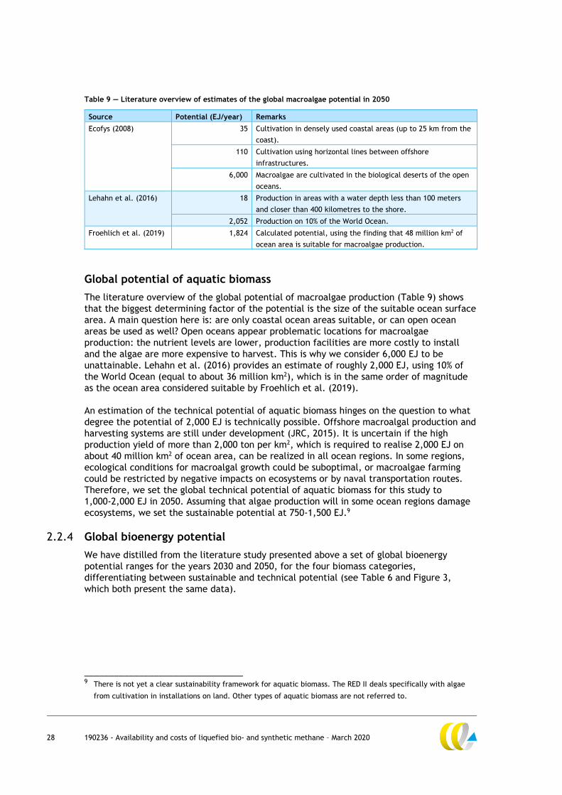
28 190236 - Availability and costs of liquefied bio- and synthetic methane – March 2020
Table 9 — Literature overview of estimates of the global macroalgae potential in 2050
Source Potential (EJ/year) Remarks
Ecofys (2008) 35 Cultivation in densely used coastal areas (up to 25 km from the
coast).
110 Cultivation using horizontal lines between offshore
infrastructures.
6,000 Macroalgae are cultivated in the biological deserts of the open
oceans.
Lehahn et al. (2016) 18 Production in areas with a water depth less than 100 meters
and closer than 400 kilometres to the shore.
2,052 Production on 10% of the World Ocean.
Froehlich et al. (2019) 1,824 Calculated potential, using the finding that 48 million km2 of
ocean area is suitable for macroalgae production.
Global potential of aquatic biomass
The literature overview of the global potential of macroalgae production (Table 9) shows
that the biggest determining factor of the potential is the size of the suitable ocean surface
area. A main question here is: are only coastal ocean areas suitable, or can open ocean
areas be used as well? Open oceans appear problematic locations for macroalgae
production: the nutrient levels are lower, production facilities are more costly to install
and the algae are more expensive to harvest. This is why we consider 6,000 EJ to be
unattainable. Lehahn et al. (2016) provides an estimate of roughly 2,000 EJ, using 10% of
the World Ocean (equal to about 36 million km2), which is in the same order of magnitude
as the ocean area considered suitable by Froehlich et al. (2019).
An estimation of the technical potential of aquatic biomass hinges on the question to what
degree the potential of 2,000 EJ is technically possible. Offshore macroalgal production and
harvesting systems are still under development (JRC, 2015). It is uncertain if the high
production yield of more than 2,000 ton per km2, which is required to realise 2,000 EJ on
about 40 million km2 of ocean area, can be realized in all ocean regions. In some regions,
ecological conditions for macroalgal growth could be suboptimal, or macroalgae farming
could be restricted by negative impacts on ecosystems or by naval transportation routes.
Therefore, we set the global technical potential of aquatic biomass for this study to
1,000-2,000 EJ in 2050. Assuming that algae production will in some ocean regions damage
ecosystems, we set the sustainable potential at 750-1,500 EJ.9
2.2.4 Global bioenergy potential
We have distilled from the literature study presented above a set of global bioenergy
potential ranges for the years 2030 and 2050, for the four biomass categories,
differentiating between sustainable and technical potential (see Table 6 and Figure 3,
which both present the same data).
________________________________ 9 There is not yet a clear sustainability framework for aquatic biomass. The RED II deals specifically with algae
from cultivation in installations on land. Other types of aquatic biomass are not referred to.

29 190236 - Availability and costs of liquefied bio- and synthetic methane – March 2020
Our main approach for setting a range was to select, for each of the four categories, the
lowest value and the highest value from the various studies. When the estimates from the
studied literature for the year 2050 were below those of 2030, we have used the 2030
values. These differences may be caused by the different methodologies, as we have looked
at different studies for the year 2050 compared to the year 2030.
Regarding a maximum technical potential for energy crops in 2050, we have not used the
1,272 EJ value form Slade et al. (2014) as these authors call bioenergy potentials above
600 EJ ‘extreme’. This 600 EJ is exactly equal to the maximum technical potential in 2050
given by IPCC (2011).Therefore, we have adopted the technical energy crop potential
estimate from IPCC (2011).
A global aquatic biomass potential for the year 2030 has not been found in literature.
Many researchers state that aquatic biomass production will not yet be profitable in 2030.
Although the estimation of the economic biomass potential is out of the scope of this
analysis, we take this important observation — which has such a large influence on the
supply of aquatic biomass — into account. Therefore, we estimate the aquatic biomass
potential in 2030 well below the values that would be obtained when interpolating the 2050
estimations.
Table 10 — Estimation of global primary bioenergy potentials for 2030 and 2050 (EJ)
Biomass category Technical
potential in
2030
Sustainable
potential in
2030
Technical
potential in
2050
Sustainable
potential in
2050
Energy crops 25-90 25-40 25-330 25-110
Agricultural residues 25-190 10-65 25-560 10-65
Forestry products and residues 30-70 25-40 45-265 25-40
Aquatic biomass 50-100 50-100 1,000-2,000 750-1,500
Total (with aquatic biomass) 130-450 110-245 1,095-3,155 810-1,715
Total (without aquatic biomass) 80-350 60-145 95-1,155 60-215
Figure 7 — Estimation of global primary bioenergy potentials for 2030 and 2050 (EJ)

30 190236 - Availability and costs of liquefied bio- and synthetic methane – March 2020
Figure 7 illustrates that the worldwide maximum sustainable bioenergy potential could
become higher than 2,000 EJ in 2050 if aquatic biomass is accounted for. To put this into
perspective: The global primary energy supply in 2015 was 571 EJ, and the current
contribution of biomass to bioenergy consumption worldwide is about 50 EJ. Thus, the
global bioenergy production in 2050 could become more than 40 times than today, if the
potential is utilised.
Secondly, the global bioenergy potential might increase dramatically between 2030 and
2050. The potential in 2050 could be more than eight times higher in 2050 than in 2030,
according to our assessment.
A third observation is that the estimated sustainable bioenergy potential is about half of the
technical potential. When aquatic biomass is disregarded, the sustainable bioenergy
potential is approximately 40% of the technical potential in 2030 and 20% in in 2050.
Fourth, aquatic biomass could play a major role in 2050, and bring back the relative
contribution of land-based biomass (energy crops, agricultural residues and forestry
products and residues) from 55-80% in 2030 to 5-35% in 2050. When only considering the
sustainable potential, the share of land-based biomass would be approximately 60% in 2030
and 15% in 2050.
2.2.5 Production capacity
The global bioenergy production potential estimated for 2030 and 2050 in the last
subsection, can only be realised if there is sufficient production capacity. For LBM
production this includes production capacity for anaerobic digestion and biogas upgrading
(for the anaerobic digestion route), gasification and methanation (for the gasification route)
and liquefaction. According to Cedigaz (2019), biomethane production has risen
exponentially since 2010, up to 3 billion m3 in 2017 (Cedigaz, 2019).This is equal to a total
energy value (based on the HHV of biomethane) of 0.12 EJ. According to Tybirk (2018), the
current annual production capacity of LBM is 0.044 Mt, corresponding to 56 million m3 of
biomethane (or 0.002 EJ). Noticing that the minimum global bioenergy production potential
in 2030 is 110 EJ (see Table 10), the current production capacity is only a fraction of the
capacity needed to utilize the bioenergy production potential.
All of these systems could be built well within ten years. Whether these systems will
actually be built primarily depends on their profitability. In turn, the profitability depends
on the cost price of LBM and the selling price to ship operators and other customers in 2030
and 2050. Additionally, the relative profitability compared to other energy investments is a
relevant factor. The LBM cost price will be discussed in Section 2.3. For the estimation of
maximum conceivable supply we will assume that the required production capacity will be
present, but with the remark that this will depend on the business case for investments in
LBM production.
2.2.6 Production yield
In order to calculate the maximum conceivable LBM production from the potential available
biomass for bioenergy, we need to know the production yield of different technology-
feedstock combinations, in kilogram of biomethane per ton of dry matter. We present this
information in Table 11.

31 190236 - Availability and costs of liquefied bio- and synthetic methane – March 2020
Table 11 — Biomethane production yields for different technology-feedstock combinations
Conversion route Technology Feedstock Biomethane
production yield
(kg biomethane /
ton dry matter of
feedstock)
Used source*
Anaerobic
digestion
Manure digestion Cattle slurry 86-216 NNFCC (2019)
Pig slurry 108-270
Co-digestion Manure + plant-
based biomass
150-300** Estimation by CE Delft
All-feedstock
digestion
Whole wheat crop 322-484 NNFCC (2019)
Maize silage 348-575
Sugar beet 136-329
Straw 139-279
Sorted food waste 355-533 SGC (2012)
Sludge 173-259
Seaweed 120-306 Milledge et al. (2019)
Microalgae 94-450
Dry digestion Not found Not found
Thermal Pressure
Hydrolysis (TPH)
Not found Not found
Autogenerative
High Pressure
Digestion (AHPD)
Not found Not found
Gasification Wood gasification Wood 140-210 Göteborg Energi (2018)
Woody biomass 135-140 CE Delft (2018c)
Woody biomass 135-140 CE Delft (2018c)
Woody biomass 135-140 CE Delft (2018c)
Plasma gasification Not found Not found
Supercritical water
gasification
Microalgae 288 CE Delft (2019)
Sewage sludge 203
Chicken manure 225
* Values have been calculated assuming a biomethane content in biogas of 50-75% (CE Delft, 2018c), no
biomethane losses in the liquefaction process, and a calorific value of methane of 55.40 MJ/kg (HHV).
** Own estimation, based on the assumption that co-digesters use 50% manure and 50% plant-based biomass.
For various new technologies, information on suitable feedstocks and production yields has
not been found in the literature. However, it is uncertain if these new technologies are
ready for commercial application in 2030/2050 and whether they will be cost-competitive.
We continue the analysis with existing technologies for which we have an estimation of the
biomethane production yield, and for which we can find cost data for Section 2.3.
For the purpose of calculating the maximum conceivable supply of LBM, we adopt the
conversion technology with the highest production yield for each of the four biomass
categories used in this analysis (see Table 12).

32 190236 - Availability and costs of liquefied bio- and synthetic methane – March 2020
Table 12 — Technologies and maximum biomethane production yields assumed in this study
Biomass feedstock categories Technology Maximum biomethane yield
(kg/ton dry matter)
Energy crops Anaerobic digestion 250-300
Agricultural residues Anaerobic digestion 250-300
Forestry products and residues Wood gasification 140-210
Aquatic biomass Anaerobic digestion 250-300
We have derived a maximum production yield range for each of the four biomass categories
from Table 11, considering the maximum yield values for different types of feedstock within
each of the biomass feedstock categories.
Although wet biomass could also be processed by supercritical gasification, the production
yields of anaerobic digestion appear higher. Moreover, anaerobic digestion is an operational
technology, and therefore yields and cost levels are more certain.
2.2.7 Maximum conceivable supply of LBM
Finally, we can calculate the maximum conceivable supply of LBM worldwide in 2030 and
2050. To this end we have used the bioenergy potentials from Table 10, factors to convert
the energy content of the biomass feedstocks into kilograms dry matter and the production
yields from Table 12. The minimum value of the maximum conceivable supply has been
calculated by taking the minimum biomethane production yield, and the maximum
conceivable supply value by using the maximum production yield. The resulting maximum
conceivable supply ranges of LBM are given in Table 13 (in Mt) and Table 14 (in EJ).
The same data are graphically presented in Figure 8 (Mt).
Table 13 — Global maximum conceivable supply of LBM in 2030 and 2050 (Mt)
Biomass category Technical
potential in
2030
Sustainable
potential in
2030
Technical
potential in
2050
Sustainable
potential in
2050
Energy crops 350-1,500 350-650 350-5,450 350-1,800
Agricultural residues 350-3,150 150-1,100 350-9,300 150-1,100
Forestry products and residues 200-750 200-400 300-2,800 200-400
Aquatic biomass 650-1,600 650-1,600 13,150-31,600 9,850-23,700
Total (with aquatic biomass) 1,600-7,000 1,300-3,700 14,200-49,100 10,500-27,000
Total (without aquatic biomass) 900-5,400 650-2,200 1000-17,600 650-3,300
Table 14 — Global maximum conceivable supply of LBM in 2030 and 2050 (EJ)
Biomass category Technical
potential in
2030
Sustainable
potential in
2030
Technical
potential in
2050
Sustainable
potential in
2050
Energy crops 19-83 19-37 19-303 19-101
Agricultural residues 19-174 8-60 19-514 8-60
Forestry products and residues 12-41 10-24 18-156 10-24
Aquatic biomass 36-87 36-87 729-1,749 547-1,312
Total (with aquatic biomass) 86-386 73-207 785-2,722 583-1,496
Total (without aquatic biomass) 50-298 37-120 56-973 37-184
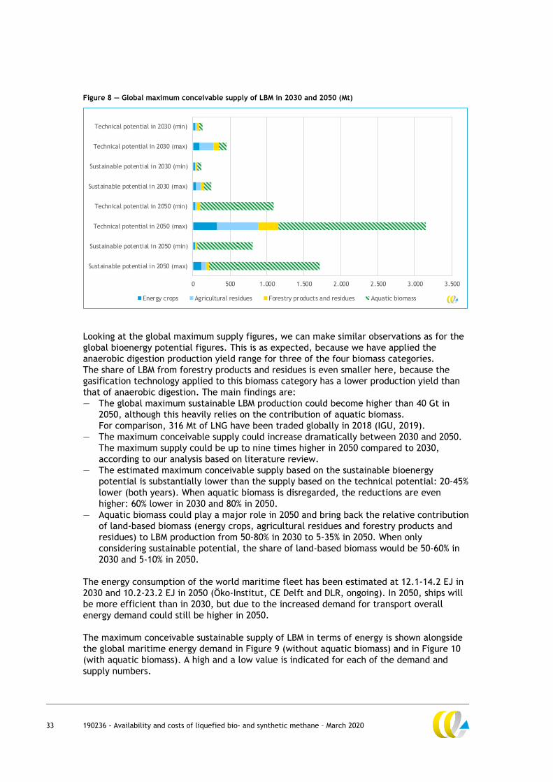
33 190236 - Availability and costs of liquefied bio- and synthetic methane – March 2020
Figure 8 — Global maximum conceivable supply of LBM in 2030 and 2050 (Mt)
Looking at the global maximum supply figures, we can make similar observations as for the
global bioenergy potential figures. This is as expected, because we have applied the
anaerobic digestion production yield range for three of the four biomass categories.
The share of LBM from forestry products and residues is even smaller here, because the
gasification technology applied to this biomass category has a lower production yield than
that of anaerobic digestion. The main findings are:
— The global maximum sustainable LBM production could become higher than 40 Gt in
2050, although this heavily relies on the contribution of aquatic biomass.
For comparison, 316 Mt of LNG have been traded globally in 2018 (IGU, 2019).
— The maximum conceivable supply could increase dramatically between 2030 and 2050.
The maximum supply could be up to nine times higher in 2050 compared to 2030,
according to our analysis based on literature review.
— The estimated maximum conceivable supply based on the sustainable bioenergy
potential is substantially lower than the supply based on the technical potential: 20-45%
lower (both years). When aquatic biomass is disregarded, the reductions are even
higher: 60% lower in 2030 and 80% in 2050.
— Aquatic biomass could play a major role in 2050 and bring back the relative contribution
of land-based biomass (energy crops, agricultural residues and forestry products and
residues) to LBM production from 50-80% in 2030 to 5-35% in 2050. When only
considering sustainable potential, the share of land-based biomass would be 50-60% in
2030 and 5-10% in 2050.
The energy consumption of the world maritime fleet has been estimated at 12.1-14.2 EJ in
2030 and 10.2-23.2 EJ in 2050 (Öko-Institut, CE Delft and DLR, ongoing). In 2050, ships will
be more efficient than in 2030, but due to the increased demand for transport overall
energy demand could still be higher in 2050.
The maximum conceivable sustainable supply of LBM in terms of energy is shown alongside
the global maritime energy demand in Figure 9 (without aquatic biomass) and in Figure 10
(with aquatic biomass). A high and a low value is indicated for each of the demand and
supply numbers.
0 500 1.000 1.500 2.000 2.500 3.000 3.500
Sustainable potential in 2050 (max)
Sustainable potential in 2050 (min)
Technical potential in 2050 (max)
Technical potential in 2050 (min)
Sustainable potential in 2030 (max)
Sustainable potential in 2030 (min)
Technical potential in 2030 (max)
Technical potential in 2030 (min)
Energy crops Agricultural residues Forestry products and residues Aquatic biomass
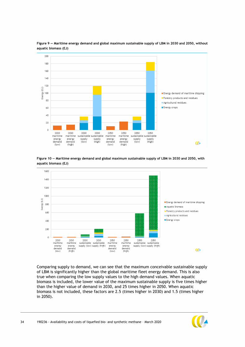
34 190236 - Availability and costs of liquefied bio- and synthetic methane – March 2020
Figure 9 — Maritime energy demand and global maximum sustainable supply of LBM in 2030 and 2050, without
aquatic biomass (EJ)
Figure 10 — Maritime energy demand and global maximum sustainable supply of LBM in 2030 and 2050, with
aquatic biomass (EJ)
Comparing supply to demand, we can see that the maximum conceivable sustainable supply
of LBM is significantly higher than the global maritime fleet energy demand. This is also
true when comparing the low supply values to the high demand values. When aquatic
biomass is included, the lower value of the maximum sustainable supply is five times higher
than the higher value of demand in 2030, and 25 times higher in 2050. When aquatic
biomass is not included, these factors are 2.5 (times higher in 2030) and 1.5 (times higher
in 2050).

35 190236 - Availability and costs of liquefied bio- and synthetic methane – March 2020
In conclusion, when assuming that the full global sustainable biomass potential in 2030 and
2050 is available for maritime shipping, the supply of LBM is more than sufficient to satisfy
the global demand of the global maritime fleet.
2.3 Cost analysis
The cost price of LBM as bunker fuel is determined by the following cost factors:
1. Biomass feedstock costs.
2. Capital and operating costs related to the production of biomethane.
3. Liquefaction costs.
4. Transport costs.
5. Bunker infrastructure costs.
In the next paragraphs we will first present an overview of cost price estimations for
biomethane at plant, i.e. estimations considering the first two cost factors as listed above
(see Section 2.3.1). This is followed by more detailed information on the different
underlying cost factors and their potential future development (see Section 2.3.2). The last
three costs items, i.e. liquefaction, transport and bunker infrastructure costs, are relevant
both for LBM and LSM and will be discussed in chapter 4 where we also compare the costs of
different bunker fuel types.
2.3.1 Production costs of biomethane
Table 15 gives an overview of the estimates of biomethane production costs, differentiated
by conversion route, as can be found in the literature. The estimations include feedstock
costs and represent either current or 2050 costs. For 2030 we were not able to find cost
estimations in the literature. For comparability reasons, we have converted the estimations
to 2019 USD per MMBtu. In the footnotes to Table 15, specific assumptions in the different
studies are highlighted.
Table 15 — Biomethane cost price values (USD2019/MMBtu) at plant as can be found in the literature
(current and 2050)
Source Anaerobic digestion Gasification
Current situation
Billig (2016) 24-63 a
BIOSURF (2016) 28-42b
Cucchiella et al. (2015) 25-49c
EA Energianalyse and SDU (2016) 20-27d
CE Delft et al. (2016) 25
Ecofys (2018) 33
Gassner and Maréchal (2009) 39-52 e
IRENA (2018b) 9-30f
Navigant (2019) 19 33
2050
Ecofys (2018) 21 13
Navigant (2019) 15g
a: The cost range results from the influence of plant capacity and feedstock use. b: 0.80 EUR/m3
for a production capacity of 500 m3/hour and 1.20 EUR/m3 for a capacity of 80 m3/hour.
c: The cost value of 0.71 EUR/m3 is for a 1,000 m3/h biomethane plant using 30% energy crops and 70% livestock
slurry. The value of 1.42 EUR/m3 is for a 100 m3/h plant using energy crops. Compression and distribution costs
are included in these values.
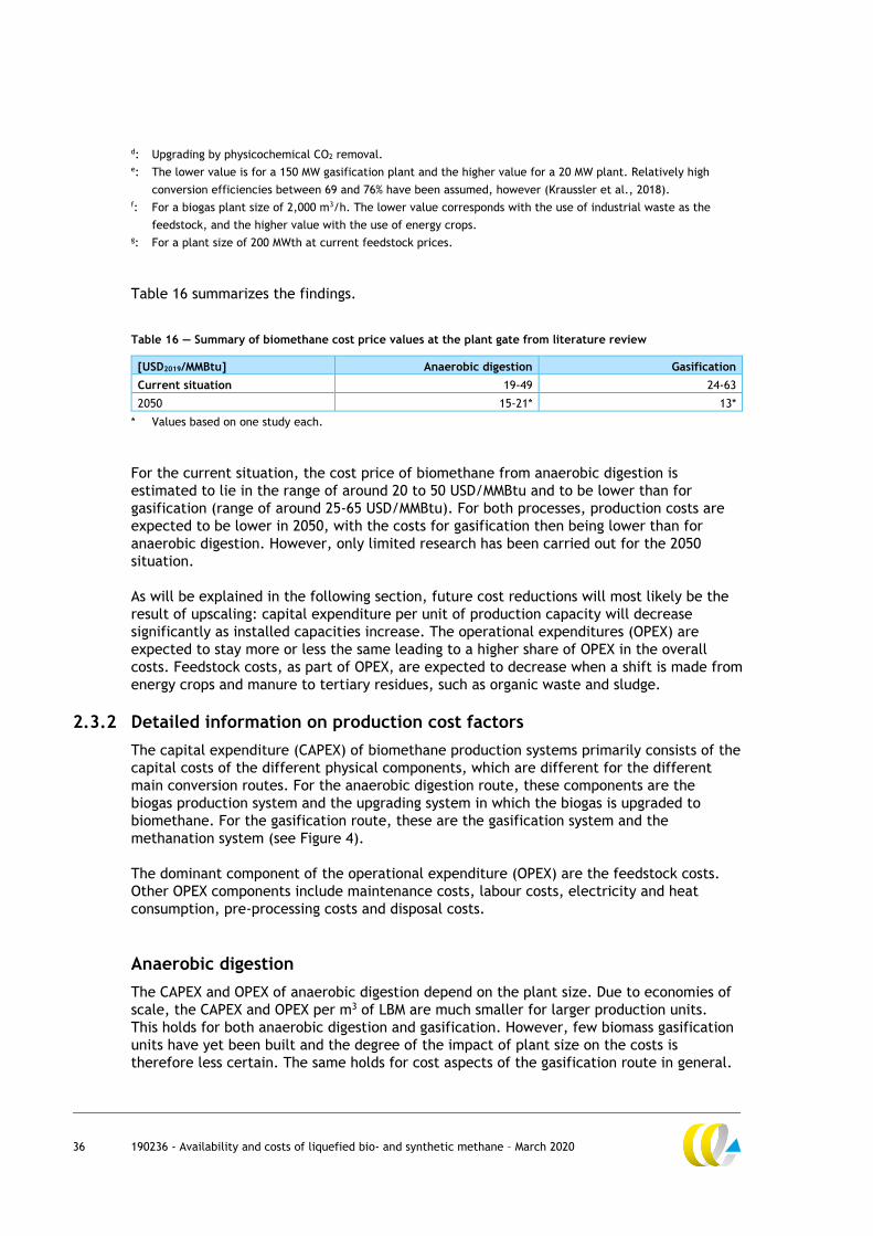
36 190236 - Availability and costs of liquefied bio- and synthetic methane – March 2020
d: Upgrading by physicochemical CO2 removal. e: The lower value is for a 150 MW gasification plant and the higher value for a 20 MW plant. Relatively high
conversion efficiencies between 69 and 76% have been assumed, however (Kraussler et al., 2018). f: For a biogas plant size of 2,000 m3/h. The lower value corresponds with the use of industrial waste as the
feedstock, and the higher value with the use of energy crops. g: For a plant size of 200 MWth at current feedstock prices.
Table 16 summarizes the findings.
Table 16 — Summary of biomethane cost price values at the plant gate from literature review
[USD2019/MMBtu] Anaerobic digestion Gasification
Current situation 19-49 24-63
2050 15-21* 13*
* Values based on one study each.
For the current situation, the cost price of biomethane from anaerobic digestion is
estimated to lie in the range of around 20 to 50 USD/MMBtu and to be lower than for
gasification (range of around 25-65 USD/MMBtu). For both processes, production costs are
expected to be lower in 2050, with the costs for gasification then being lower than for
anaerobic digestion. However, only limited research has been carried out for the 2050
situation.
As will be explained in the following section, future cost reductions will most likely be the
result of upscaling: capital expenditure per unit of production capacity will decrease
significantly as installed capacities increase. The operational expenditures (OPEX) are
expected to stay more or less the same leading to a higher share of OPEX in the overall
costs. Feedstock costs, as part of OPEX, are expected to decrease when a shift is made from
energy crops and manure to tertiary residues, such as organic waste and sludge.
2.3.2 Detailed information on production cost factors
The capital expenditure (CAPEX) of biomethane production systems primarily consists of the
capital costs of the different physical components, which are different for the different
main conversion routes. For the anaerobic digestion route, these components are the
biogas production system and the upgrading system in which the biogas is upgraded to
biomethane. For the gasification route, these are the gasification system and the
methanation system (see Figure 4).
The dominant component of the operational expenditure (OPEX) are the feedstock costs.
Other OPEX components include maintenance costs, labour costs, electricity and heat
consumption, pre-processing costs and disposal costs.
Anaerobic digestion
The CAPEX and OPEX of anaerobic digestion depend on the plant size. Due to economies of
scale, the CAPEX and OPEX per m3 of LBM are much smaller for larger production units.
This holds for both anaerobic digestion and gasification. However, few biomass gasification
units have yet been built and the degree of the impact of plant size on the costs is
therefore less certain. The same holds for cost aspects of the gasification route in general.

37 190236 - Availability and costs of liquefied bio- and synthetic methane – March 2020
Navigant (2019) provides CAPEX and OPEX costs for different plant sizes (500 m3/h and
1,000 m3/h) and a upgrading unit of 1,000m3/h (see Table 17).
Table 17 — CAPEX and OPEX for anaerobic digestion for the current situation (Navigant, 2019)
Technology Plant size (m3/h) CAPEX (MEUR) OPEX (MEUR/yr) Biomethane yield
(m3/t dry matter)
Anaerobic digestion 500 5.86 0.60 Feedstock specific
Anaerobic digestion 1,000 9.89 0.63 Feedstock specific
Anaerobic digestion
(upgrading unit only)
1,000 2.00 0.11 Not applicable
According to SGAB (2017) both the capital and operational costs (other than the feedstock
costs) lie in the same range of 10-15% of total cost. Other costs are likely to consist of
feedstock cost. A main cost driver for the non-feedstock related OPEX costs is the heat
required for the various production steps. The relative share of non-feedstock related OPEX
costs can decline as result of scale effects. For example, SGAB (2017) mentions that staffing
requirements are independent of the capacity: whereas these costs might form the
dominant cost at smaller capacities, this will be different for larger production units.
Ecofys (2018) gives the composition of CAPEX, feedstock costs and other OPEX for
biomethane produced through anaerobic digestion in the current situation and in 2050
(Table 18). The cost reduction between 2050 and today arises from process efficiency
improvements, larger digestion units (from < 2 MW units to 6 MW units) and larger upgrading
units that process the biogas from multiple digestion units. An increase in feedstock costs
has been assumed, because the potential of low-cost biomass residues was thought to be
‘significant, yet still limited’. Also, the use of sequential crops10 is assumed in 2050, which
are relatively costly (Ecofys, 2018).
Table 18 — Composition of CAPEX and OPEX of anaerobic digestion in current situation and in 2050 (Ecofys,
2018)
Cost Value Current situation a 2050
Full cost
CAPEX (MEUR/MW) 5.63 1.84
OPEX excl. feedstock cost
(% of CAPEX)
6-10% 6-10%
Levelized cost (EUR/MWh of biomethane)
CAPEX 41 (43%) 13 (22%)
OPEX excl. feedstock cost 44 (46%) 25 (42%)
Feedstock cost 11 (11%) 22 (37%)
Total cost 96 (100%) 60 (100%)
a: Data for the year 2015.
________________________________ 10 Triticale and maize silage are assumed to be produced as sequential crops, i.e., “as additional (second) crop
before or after the harvest of main crops on the same agricultural land” (Ecofys, 2018).

38 190236 - Availability and costs of liquefied bio- and synthetic methane – March 2020
Tsiropoulos et al. (2018) provide CAPEX figures of anaerobic digestion for the current
situation, 2030 and 2050 (see Table 19). The current CAPEX value is lower as the one from
Ecofys (2018). Comparing CAPEX reductions over time, Tsiropoulos et al. (2018) give a
reduction between today and 2050 of 5-26%, whereas the reduction given by Ecofys (2018)
is 67%. However, since the current CAPEX value of Ecofys (2018) is higher, the 2050
estimates of both sources are not that much apart. The CAPEX cost reduction between
today and 2030 of Tsiropoulos et al. (2018) is 3-16%. The relative CAPEX cost reduction
between today and 2050 is 0.2-0.7% per year (compared to 1.9% in Ecofys (Ecofys, 2018)).
Table 19 — Composition of CAPEX and OPEX of anaerobic digestion in current situation, 2030 and in 2050
Cost Value Current situation a 2030 2050
Full cost
CAPEX (MEUR/MW) 3.10 2.60-3.00 2.29-2.93
OPEX excl. feedstock cost (% of CAPEX) 4% 4% 4%
Source: (Tsiropoulos et al, 2018). a: Data for the year 2015.
Energy consumption costs
Typically, 5 to 10% of the energy of the biogas produced in anaerobic digestion systems is
needed for heating the digesters — other energy sources could of course also be used for
this. Furthermore, the consumption of electricity, which is used to power pumps and
monitoring and control systems, is typically 20 to 30 kWhe per MWh of biogas (IRENA,
2018b).
Gasification
Gasification units are currently less technically mature than anaerobic digestion units.
Capital costs are high due to the early stage of development, but significant cost reductions
can be expected due to innovations, technology scale-up and continuous deployment.
Table 20 provides cost estimates for a first of a kind plant as well as for ‘Nth of a kind’
plants of various sizes. Based on this table, a 50% reduction of CAPEX is expected for a large
‘Nth of a kind’ gasification plant compared to a first of a kind plant that is five times
smaller. OPEX are also expected to decrease by 50%. Navigant (2019) mentions improved
plant integration, innovative gas cleaning methods and high-pressure gasification as
potential other factors that might contribute to a reduction of overall system costs, but
these cost reductions have not been quantified in the OPEX costs as depicted in Table 20.
Table 20 — CAPEX and OPEX for gasification
Technology Plant size
(MWth)
CAPEX
(EUR/MWth)
OPEX
(MEUR/MWth/year)
Energy efficiency
(%)
Gasification (first of a kind) 42 2.83 0.27 64%
Gasification (Nth of a kind) 42 2.41 0.25 64%
Gasification (Nth of a kind) 84 1.98 0.22 64%
Gasification (Nth of a kind) 200 1.4 0.15 75%
Source: (Navigant, 2019).

39 190236 - Availability and costs of liquefied bio- and synthetic methane – March 2020
Table 21 provides the CAPEX and OPEX of gasification in 2050 as estimated by Ecofys (2018).
The levelized cost of biomethane produced by gasification in 2050 are 37% lower than the
estimated value for biomethane produced by anaerobic digestion. The main reason is the
difference in assumed biomethane production yields: 0.55 m3 of biomethane/kg of
feedstock for gasification vs. 0.36 m3/kg for anaerobic digestion. Also, the operation
and maintenance cost and CAPEX of anaerobic digestion are higher (Ecofys, 2018).
Table 21 — Composition of CAPEX and OPEX of gasification in 2050 (Ecofys, 2018)
Cost Value 2050
Full cost
CAPEX (MEUR/MWth)11 1.64
OPEX excl. feedstock cost (% of CAPEX) 5%
Levelized cost (EUR/MWh of biomethane)
CAPEX 13 (34%)
OPEX excl. feedstock cost 12 (32%)
Feedstock cost 13 (34%)
Total cost 38 (100%)
Navigant (2019) estimates the CAPEX of a first of a kind gasification plant at
2.83 MEUR/MWth. Assuming a CAPEX of 1.64 MEUR/MW from Ecofys in 2050, the cost
reduction would be 42%, or ~1.2%/year. Interpolating for 2030, the CAPEX of a gasification
plant in 2030 would be ~2.3 MEUR/MW.
Upgrading costs
According to CE Delft et al. (2016) biogas upgrading costs are 0.2-0.31 EUR/m3 biomethane,
but these decrease with increasing scale to 0.13 EUR/m3 at a production capacity of 2,000
m3/hour. This is comparable to IRENA (2018b), which shows a reduction of 0.2-0.3 USD/m3
of biomethane at a production capacity of 250 m3/hour to 0.1-0.15 USD/m3 at 2,000
m3/hour. In the case of smaller upgrading units, the upgrading cost can reach 1.0 USD/m3.
The upgrading costs can also be considered to include the (capital and operational) cost of
transport of the raw biogas to the upgrading facility. Navigant (2019) estimates the costs for
biogas pipelines at 5 EUR/MWh (0.06 EUR/m3).
Feedstock costs
According to Lambert (2017), biomethane produced from manure and industrial waste
processed in larger installations are nearly competitive, but biomethane plants using
expensive feedstocks are uncompetitive without any governmental support closing the gap.
However, due to the large variety in potential feedstock for anaerobic digestion plants,
feedstock costs could range from negative (in case of waste streams that have a disposal
cost) up to 100 EUR/ton for straw (SGAB, 2017). Figure 11 shows the current cost structure
of biomethane production for various feedstock groups and for different scales of
production.
________________________________ 11 Based on the source it was not clear to what extent whether this figure represented MWth (thermal energy of
biomass). We have assumed this is the case, which has resulted in a somewhat lower figure than when
MWbiomethane would have been assumed.

40 190236 - Availability and costs of liquefied bio- and synthetic methane – March 2020
Figure 11 — Total production costs for biomethane from anaerobic digestion by feedstock and size for the
current situation
Source: (IRENA, 2018b).
In Table 22, the costs of different biomass feedstocks for the current situation, 2030 and
2050 are indicated, based on various literature sources.
Table 22 — Feedstock costs per feedstock type (current, 2030 and 2050)
Feedstock category Feedstock type Current
(EUR Cent/kWh)3
2030 (USD/GJ) 2 2050 (EUR/tonne
dry matter)1,4
Energy crops Maize, sugar cane,
wheat
8.5 4-80 78-90
Agricultural
residues
Crop residues 8.5 3-8 47-61
Manure 6.3 n.a. 5-50
Woody residues Bark, branches,
tops, early thinnings
4.9
1-20 92
Residual and post-
consumer waste
MSW 6.5 n.a. 12
Wood waste n.a. 1-20 12
1: Navigant (2019). 2: IRENA (2018b). Includes the costs of production, collection and transport of biomass. 3: Trinomics et al. (2019). 4: Ecofys (2018).

41 190236 - Availability and costs of liquefied bio- and synthetic methane – March 2020
Woody residues can only be converted to biomethane through gasification. The other
feedstocks can currently only be used in digesters. With supercritical water gasification,
digestible feedstocks could also be gasified, but cost figures on this new technology are still
lacking. Here we focus our attention on anaerobic digestion and conventional (thermal)
gasification, the technologies that also have been included in the availability analysis of
Section 2.2.
In Figure 12 the production costs of biomethane from various feedstocks are depicted.
It shows that the costs can vary substantially, depending on the feedstock: up to
50 EUR/MWh, when comparing organic waste to manure, amounting to ~50% of the total
production cost.
This can be explained by the different cost prices of the feedstocks, but also by other
indirect effects of the different feedstock types on the OPEX: The choice of feedstock
affects for example the value or cost of disposal of the digestate. Furthermore, the gas
yield from the variety of substrates may in practice range from 150 to 600 m3/ton dry
substance (SGAB, 2017). A higher production yield results in a lower feedstock input volume
per m3 of liquid biomethane.
According to a survey among biogas plant operators in the EU (BIOSURF, 2016), the
contribution of feedstock costs lies in a range of 3 to 60 EUR/MWh.
Figure 12 — Cost of production of biomethane from different feedstocks in the current situation
Source: (SGAB, 2017).

42 190236 - Availability and costs of liquefied bio- and synthetic methane – March 2020
3 Availability and cost price of
liquefied synthetic methane
(LSM)
This section identifies the essential elements for the potential conversion routes of
liquefied synthetic methane (LSM) and analyses their availability and their costs. We will
analyse the availability of LSM in Section 3.2 and cost price of LSM in Section 3.3.
The conversion routes that are taken into account are presented in Section 3.1, in the
scoping analysis.
3.1 Scoping analysis
We define synthetic methane as methane derived from synthesis of CO2 and hydrogen.
Synthetic methane is also known as power to gas or e-methane due to the fact that the
source of production relies on electricity and due to its substitutable properties with
natural gas, but for consistency purposes, we shall use the term LSM throughout this report.
A schematic overview of the conversion routes is depicted in Figure 13.
Figure 13 — Potential conversion route for the production of LSM

43 190236 - Availability and costs of liquefied bio- and synthetic methane – March 2020
Electricity and water are feedstocks to produce hydrogen via the process of electrolysis.
In a methanation process, the produced hydrogen can, using CO2, be converted into
methane. For storage and use by ships, the methane needs to be liquefied.
For each step in the production various options exists. These options will be described in
more detail in the next sections and will be limited to the options included in the scope of
this study.
3.2 Availability analysis
The analysis of the availability of LSM differs fundamentally from the analysis of the
availability of LBM. In contrast to the biomass feedstocks required for the production of
LBM, the main inputs required for the production of renewable LSM (electricity, water and
CO2) are technically not restricted. The effective technical potential of LSM will be
determined by the availability of (excess) renewable electricity which is very difficult to
project on a global level. For this reason we decided to determine the renewable electricity
required for covering the expected future energy demand of shipping by means of
renewable LSM only.
This section zooms in on the availability of renewable electricity, water, and CO2 as well as
the main relevant processes which are electrolysis, methanation and liquefaction.
3.2.1 Availability of renewable electricity
Electricity is an essential input for the production of sustainable LSM. Electricity is used for
the production of hydrogen by means of electrolysis (Figure 13) and is also required for
capturing of CO2, the methanation process, and, depending on the technology, also for the
liquefaction process. While LSM can in principle be produced with the current electricity
mix — a mix including a non-renewable share of electricity — LSM can only be used in a
decarbonised shipping sector if it is produced by means of renewable electricity.
Power-to-gas, including power-to-methane, is also considered as an option to store surplus
renewable power from wind or solar energy. This however requires, as will be discussed in
more detail below, the establishment of a production process that can cope with load
changes (Gorre, 2019). And excess renewable electricity is also not expected to be
sufficient to cover the power demand of synthetic fuel production and is probably not be an
economically viable option due to the relative low full load hours at which a plant could be
operated (Frontier Economics, 2018).
Dedicated renewable power plants would have to be used instead, requiring additional
investments, leading to relative higher electricity prices, and to additional land use.
Regarding the future availability of renewable power, there are many different projections.
The differences lie mainly in assumptions about the ambition of global climate policy. We
shall look into the following three reputable publications which have been developed or
adopted by international organisations.
One authoritative report is “Global energy transformation — A roadmap to 2050” (IRENA,
2019e). According to that report, the renewables share in electricity generation was around
20% in 2010. Using 2010 as the baseline, (IRENA, 2019e) has developed two scenarios, one is
the Reference Case where the future projections are predicted based on historical growth

44 190236 - Availability and costs of liquefied bio- and synthetic methane – March 2020
of renewable energy share in electricity and the REmap12 Case assumes that that supportive
policy and frameworks will be implemented to limit the average global surface temperature
increase to well below 2°C by 2100 and is thus commensurate with the ambitions of the
Initial IMO strategy on reduction of GHG emissions from ships.13 This scenario includes the
deployment of low carbon technologies based largely on renewable energy and energy
efficiency. Under these assumptions, the share of renewable electricity generation will
increase from approximately 24 in 2016 to 57% in 2030 and to 86% by 2050. In absolute
terms renewable electricity generation would account for around 20,400 TWh and
47,700 TWh in 2030 and 2050 respectively (see Table 23).
The International Energy Agency (IEA) has developed Energy Technology Perspectives (ETP)
for the sectors energy supply, buildings, industry and transport (IEA, 2017a). Two climate
mitigation pathways have been developed in this context: the ‘2°C Scenario’ and the
‘Beyond 2°C Scenario’. The ‘2°C Scenario’ is the ETP’s central climate mitigation scenario
and lays out an energy system pathway and a CO2 emissions trajectory consistent with an at
least 50% chance of limiting the average global temperature increase to 2°C by 2100 (IEA,
2017a). The ‘Beyond 2°C Scenario’ explores how far deployment of technologies that are
already available or in the innovation pipeline could take the world beyond the ‘2°C
Scenario’. Technology improvements and deployment are thereby assumed to be pushed to
their maximum practicable limits across the energy system in order to achieve net-zero
emissions by 2060 and to stay net zero or below thereafter, without requiring unforeseen
technology breakthroughs or limiting economic growth (IEA, 2017a). Considering both
scenarios, gross total electricity production is expected to amount to 31,000-31,400 TWh in
2030 and 42,500-44,300 TWh in 2050 and gross renewable electricity production to
14,500 TWh and 28,700-31,800 TWh in 2030 and 2050 respectively.
As part of IPCC’s Fifth Assessment Report, four representative concentration pathways,
RCP2.6; RCP4.5; RCP6.0; RCP8.5, named according to their 2100 radiative forcing levels,
have been selected to represent a broad range of climate outcomes. After the Paris
Agreement an additional RCP pathway, i.e. RCP 1.9 has been developed. From these five
pathways, RCP2.6 and RCP1.9 are the concentration pathways for which it is likely that the
temperature increase stays at/below 2°C in 2100. Five Shared Socio-Economic Pathways
(SSPs) have been developed to complement the RCPs. They describe potential major global
developments (population development, urbanization and economic development (GDP))
that together will lead to different challenges for mitigation and adaptation to climate
change (Riahi et al. 2017). The socio-economic information of the SSPs have been used as
input for runs of different integrated assessment models to determine key variables (like
e.g. energy consumption for different sectors) that match the different RCPs. Table 23
gives the expected power generation and the share of renewable electricity production for
RCP2.6 and RCP1.9 scenarios, with the range reflecting the different SSPs applied.14
As Table 23 shows, for the RCP2.6 scenarios it holds that renewable electricity production
ranges from 6,300 to 13,100 TWh and from 22,200 to 28,100 TWh in 2030 and 2050
respectively whereas for the RCP1.9 scenarios from 8,100 to 14,700 TWh in 2030 and
31,200 to 49,100 TWh in 2050.
________________________________ 12 REmap = renewable energy roadmap analysis. 13 The REmap suggests that the total share of renewable energy must rise to around two-thirds by 2050 to meet
the Paris agreement goal of limiting the surface temperature below 2°C. Under this REmap Case scenario, 65%
of the total final energy consumption will be generated using renewable energy sources. It was also assumed
that the share of electricity rises to 40% of the total final energy consumption by 2050 and assumed that there
will be a 2.8% reduction in terms of energy intensity improvement compared to 2015. 14 RCP2.6 has been modelled for SSP 1, 2, 4 and 5 and the RCP 1.9 for SSP 1, 2 and 5.

45 190236 - Availability and costs of liquefied bio- and synthetic methane – March 2020
Table 23 — Projections of global renewable electricity production (TWh)
2030 2050
Total RE RE
share
Total RE RE
share
2°C scenarios IEA, 2°C Scenario 31,400 14,500 46% 42,500 28,700 67%
IPCC RCP2.6 scenarios 37,500-43,000 6,300-13,100 17-31% 43,800-51,600 22,200-28,100 43-64%
(well) below
2°C scenarios
REmap Case 35,900 20,400 57% 55,200 47,400 86%
IEA, Beyond 2°C Scenario 31,000 14,500 47% 44,300 31,800 72%
IPCC RCP 1.9 scenarios 31,600-33,300 8,100-14,700 24-47% 35,300-69,900 31,200-49,100 70-88%
Source: (IRENA, 2019a) (IIASA, 2018); (IEA, 2017a).
Differentiating between 2°C-scenarios and (well) below2°C-scenarios, the projections
renewable electricity production can be summarized with the following ranges:
— 2°C scenarios: 6,300-14,500 TWh in 2030 and 22,200-28,700 TWh in 2050;
— (well) below 2°C scenarios: 8,100-20,400 TWh in 2030 and 31,200-49,100 TWh in 2050.15
Conclusion
The generation of renewable electricity is growing fast, but currently most of the electricity
is used directly, rather than to produce fuels such as synthetic methane. In order to
produce large quantities of synthetic methane, substantial investments in renewable,
dedicated electricity capacity would be needed.
3.2.2 Availability of hydrogen
The renewable electricity is used to produce hydrogen through electrolysis of water.
Electrolysers can be categorized based on the temperature of the process namely low-
temperature electrolysers (50-80°C) and high temperature electrolysers (700–1,000°C).
There are two technologies for low-temperature electrolysis, Alkaline Electrolysis Cells
(AEC) and Proton Exchange Membrane (PEM), and one for high temperature analysis: Solid
oxide electrolysis cell (SOEC) (Table 24).
Table 24 — Electrolysis technologies
Class Technology
Low temperature electrolysis Alkaline electrolysis cells (AEC) Proton exchange membrane (PEM)
High temperature electrolysis Solid oxide electrolysis cell (SOEC)
AEC and PEM electrolysers are commercially available and can thus be considered to be
technologically mature (TRL 9). SOEC is still in the developmental stage (Frontier
Economics, 2018). There are pilot plants in Dresden, Germany and in Mellach, Austria
(Sunfire, 2019).
________________________________ 15 We interpret the renewable electricity scenarios as not accounting for the production of e-fuels to be used in
the transport sector, but this is not entierly clear. (IEA, 2017a) for example differentiates between oil, natural
gas, electricity, biomass and hydrogen regarding the final energy demand of the transport sector, but it is not
clear whether this is green or blue hydrogen.
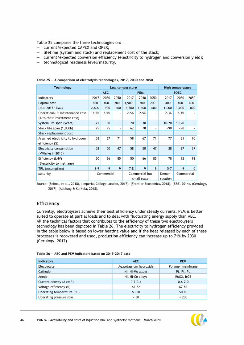
46 190236 - Availability and costs of liquefied bio- and synthetic methane – March 2020
Table 25 compares the three technologies on:
— current/expected CAPEX and OPEX;
— lifetime (system and stack) and replacement cost of the stack;
— current/expected conversion efficiency (electricity to hydrogen and conversion yield);
— technological readiness level/maturity.
Table 25 — A comparison of electrolysis technologies, 2017, 2030 and 2050
Technology Low temperature High temperature
AEC PEM SOEC
Indicators 2017 2030 2050 2017 2030 2050 2017 2030 2050
Capital cost
(EUR 2015/ kWe)
600–
2,600
400–
900
200–
600
1,900–
3,700
300-
1,300
200-
600
400–
1,000
400-
1,000
400-
800
Operational & maintenance cost
(% to their investment cost)
2-5% 2-5% - 2-5% 2-5% - 2-3% 2-3% -
System life span (years) 25 30 - 20 30 - 10-20 10-20 -
Stack life span (1,000h) 75 95 - 62 78 - <90 <90 -
Stack replacement cost
Assumed electricity to hydrogen
efficiency (%)
58 67 71 58 67 71 77 81 90
Electricity consumption
(kWh/kg in 2015)
58 50 47 58 50 47 38 37 37
Efficiency (LHV)
(Electricity to methane)
50 66 85 50 66 85 78 92 92
TRL (Assumption) 8-9 9 9 7-8 9 9 5-7 9 0
Maturity Commercial Commercial but
small scale
Demon-
stration
Commercial
Source: (Selma, et al., 2018), (Imperial College London, 2017), (Frontier Economics, 2018), (E&E, 2014), (Cerulogy,
2017), (Adelung & Kurkela, 2018).
Efficiency
Currently, electrolysers achieve their best efficiency under steady currents. PEM is better
suited to operate at partial loads and to deal with fluctuating energy supply than AEC.
All the technical factors that contributes to the efficiency of these two electrolysers
technology has been depicted in Table 26. The electricity to hydrogen efficiency provided
in the table below is based on lower heating value and If the heat released by each of these
processes is recovered and used, production efficiency can increase up to 71% by 2030
(Cerulogy, 2017).
Table 26 — AEC and PEM indicators based on 2015–2017 data
Indicators AEC PEM
Electrolyte Aq.potassium hydroxide Polymer membrane
Cathode Ni, Ni-Mo alloys Pt, Pt, Pd
Anode Ni, Ni-Co alloys RuO2, IrO2
Current density (A cm-2) 0.2–0.4 0.6-2.0
Voltage efficiency (%) 62-82 67-82
Operating temperature (°C) 60–80 50–80
Operating pressure (bar) < 30 < 200

47 190236 - Availability and costs of liquefied bio- and synthetic methane – March 2020
Indicators AEC PEM
Production rate (m3 H2 h-1) < 760 < 240
Gas purity (%) > 99.5 99.99
Cold start time (min) < 60 < 20
System (start time) Seconds Milliseconds
Stack life time (Years) 7-10 2–7
Systematic lifetime (years) 20 20
Electricity to hydrogen efficiency (%) 58-71 58-71
TRL Level 9 7-8
Flexibility (fluctuating renewable electricity) Yes Yes
Source: (Selma, et al., 2018), (Cerulogy, 2017), (IRENA, 2018a) and (Adelung & Kurkela, 2018).
Conversion efficiency
The efficiency of low temperature electrolysis is currently at 43–69% (Selma, et al., 2018),
58% on average (Cerulogy, 2017). According to (Cerulogy, 2017), the efficiency can be
improved especially when the waste heat of methanation is used. This would make it
possible for the efficiency to improve from 58% on average in 2015 to 67% in 2030 and reach
up to 71% by 2050.
Capacity
To date, about 2-4% of global hydrogen supply is produced via electrolysis (IEA, 2019d)
(IRENA, 2018a). Most of this is probably produced with AEC, which are larger scale than PEM
and require lower costs (Leeuwen, 2018), (Maria Taljegard, 2016).
Conclusion
Most electrolysers currently are of the AEC type. Its main advantages compared to PEM are
low capital costs, availability of large plants sizes and long life spans. It is technologically
also more mature than SOEC (Selma, et al., 2018). PEM currently requires higher capital
costs — mainly due to the need for expensive catalysts — and the high pressures required
are more complex than AEC (Imperial College London, 2017). However, it could become
competitive with AEC in one or two decades (International Journal of Hydrogen Energy,
2017). SOEC requires less energy than low temperature technologies, but can cope less well
with fluctuating energy supply. It is expected to become commercially available in one or
two decades.
Electrolysis is currently not used to produce hydrogen in large quantities. Electrolysis
currently accounts for 2-4% of global hydrogen production (IEA, 2019d; IRENA, 2018a).
In order to produce large quantities of synthetic methane, investments in electrolysis
capacity would be needed.
3.2.3 Availability of water
Hydrogen production requires water. Methane has an overall higher water input for
electrolysis compared to methanol or syngas, because the methanation reaction requires
more hydrogen than the methanol synthesis (Ramboll et al., 2019). It requires 4.73 kg of
water per kg (Ramboll et al., 2019).

48 190236 - Availability and costs of liquefied bio- and synthetic methane – March 2020
Electrolysis of water requires fresh water, because the electrolysis of seawater generates
chlorine as an unwanted by-product.16 This means that freshwater either has to be available
or seawater needs to be desalinated. Desalination is an established technology that is
commercially available and the application is growing rapidly (Jones, et al., 2019).
Hence, water availability is not considered to be a constraint to the production of LSM.
According to (Frontier Economics, 2018), the costs of supplying water are negligibly low,
even in countries where the water has to be obtained from desalination plants. To cover
the water demand of the electrolysis process it is, to a certain extent, possible to re-use
the water which is generated as a by-product of the methanation process with the help of a
purification plant. This could further reduce the costs of water.
3.2.4 Availability of carbon dioxide
Carbon dioxide can either be captured at point sources or it can be captured from ambient
air by means of direct air capture (DAC). Only carbon capture from biogenic point sources
and DAC can be considered to be carbon neutral. This section discusses both, carbon
capture from point sources, in general and with special focus on biogenic CO2, as well as
DAC.
Carbon capture and utilization (CCU): technology readiness
The CO2 capture processes and systems are usually categorized according to their
transformation routes (Ramboll et al., 2019). Table 27 indicates the various CO2
transformation categories and their respective processes.
Table 27 — CO2 transformation routes and process description
Transformation route Process description
Chemical (non-hydrogenative) Chemical conversion of CO2 without hydrogen as a co-reactant
Chemical (hydrogenative) Chemical conversion of CO2 with hydrogen as a co-reactant
Biological CO2 conversion by photosynthesis
Electrochemical Reduction of CO2 carbon atom by adding electrons
Photochemical Reduction of CO2 carbon atom by solar energy
Inorganic Fixation of CO2 in inorganic compounds
Source: (Ramboll et al., 2019).
(Ramboll et al., 2019) analyzed more than 130 different CCU application options from
different routes and functionalities. Out of this 130 application options, 48 have a TRL of 7
or higher, of which 19 are commercially available (TRL 9). Most of the technologically
mature routes are chemical non-hydrogenative or chemical hydrogenative processes,
although there are also some inorganic CCU routes with a high TRL. Each transformation
route mentioned in the table above satisfies the purpose of capturing carbon for a certain
product such as ethanol, polyols for polyurethane (PU) foams production, etc. For synthetic
fuels production, chemical hydrogenative transformation route has been identified as the
most suitable route (Ramboll et al., 2019). Hence, carbon capture and utilization using the
chemical hydrogenative transformation route for the production of synthetic methane is
considered to be a mature technology.
________________________________ 16 Research is ongoing into catalysts that allow the use of seawater in hydrogen production, but this is still in the
research phase. See e.g. (Vos, et al., 2018).

49 190236 - Availability and costs of liquefied bio- and synthetic methane – March 2020
A pilot demonstration plant in Falkenhangen, Germany has successfully produced synthetic
methane generated by wind turbines and using CO2 that is sourced from a bio-ethanol plant.
In March 2019, an average of 14,500 kWh synthetic methane was produced per day.17
Carbon capture at point source: CO2 availability
A techno-economic analysis performed by (Naims, 2016) indicates that the global annual
CO2 supply from point sources that could be used for carbon capturing is currently
approximately 12.7 Gt. The degree of CO2 concentration of the flue gas, the purity of the
CO2 captured and the technology applied for capturing the CO2 are thereby the main
determinants of the capture costs (Ramboll et al., 2019):
— Ammonia synthesis, hydrogen production and natural gas extraction are considered
industrial processes which emit highly pure CO2 and a small share of these emissions are
already captured today. Currently, these sources account, on a global scale, for around
250 Mt of CO2 annually (Naims, 2016).
— Biogas plants, especially biogas upgrading plants, emit relatively highly concentrated
CO2, however still at a limited scale. In North America and Brazil, these CO2 emissions
are estimated to amount to around 20 Mt annually (Naims, 2016).
— Fossil fuel power stations emit a large amount of CO2 annually (around 10 Gt), but with
3 to 15% the CO2 concentration of the flue gas is however relatively low, leading to
higher capture costs when compared to the above mentioned processes (Naims, 2016).
— Energy intensive industries, like e.g. cement production and iron and steel production
also emit a significant amount of CO2, globally around 3 Gt annually. The cement
production thereby features with 14-33% a relatively high flue gas CO2 concentration
(Naims, 2016).
Direct air capture
Direct air capture (DAC) extracts CO2 from ambient air. DAC systems have the advantage
that they do not depend on CO2 point sources; they can therefore be applied anywhere,
could be integrated into an electrolysis/methanation plant (saving CO2 transportation
costs), can be upscaled whenever desired and are not dependent on the future
development of the CO2 point sources.
The energy demand and separation costs of DAC systems are however higher if compared to
systems that capture carbon at point sources. This can be explained by the relative low CO2
concentration in ambient air (around 0.04% vs. for example 3-10% and 12-15% in flue gasses
of gas and coal power plants respectively (Naims, 2016)).
Another disadvantage of DAC systems is their relative large geographical footprint (Frontier
Economics, 2018). A facility that captures 1 Mt of CO2 would for example require 2 km2 of
land (National Academics of Sciences, Engineering, and Medicine, 2018). But this might be
more an issue if DAC was used for carbon capture and storage on a large scale.
DAC is technically feasible. Different technologies have been developed and demonstration
plants have been build, some even at commercial scale. The technology can be considered
near to commercialization (GlobeNewswire , 2019).18
________________________________ 17 Store & GO : The German demonstration site at Falkenhagen 18 CO2 captured from air is intended to be used for the flooding of oil fields to extend the economic life of their
economic life.

50 190236 - Availability and costs of liquefied bio- and synthetic methane – March 2020
In DAC systems, chemical sorbents are used to remove CO2 as ambient air flows over an air
contactor. After CO2 is captured, the material used for separation requires regeneration.
(National Academics of Sciences, Engineering, and Medicine, 2018).
DAC involves two generic approaches, one being a solvent-based method and another being
solid-sorbent-based:
— In the solvent-based approach, a strong alkaline solution is used to capture CO2 from the
air in a simple acid-base reaction that results in the formation of a stable carbonate,
which then has to be heated in an oxy-fired kiln to release high-purity CO2 and lime to
be recycled throughout the process,
— In a solid-sorbent-based DAC process, CO2 from the air binds to a sorbent using a
gas-solid contactor. An approach based on both heat and vacuum is used to desorb the
CO2 from the sorbent, producing a concentrated stream of CO2. This system is
subsequently cooled to begin the cycle again (National Academics of Sciences,
Engineering, and Medicine, 2018). This process to release the CO2 captured is also
referred to as temperature swing adsorption (TSA).
According to (Frontier Economics, 2018), the most established DAC technology is
temperature swing adsorption (TSA). Table 28 captures the key indicators for direct air
capture by means of TSA and for capturing of biogenic CO2 from point sources. The data for
biogenic CO2 sources is based on the data from post and pre-combustion systems that could
separate CO2 from the flue gases produced during the production of the primary fuel.
Table 28 — Average energy use estimates for direct air capture and for CO2 capture from biogenic point
sources
Source Concentration
of CO2
Electricity demand
(MJ/kgCO2e)
Heat demand
(MJ/kgCO2e)
CAPEX
(Euro/tonne CO2)
OPEX
(% of
investment cost)
TRL
Direct air
capture
(TSA)
0.04% 0.9–1.29 4.19 41-2,086 1.5-4% 7
CCU 10–100% 0.03–0.11 1.3–3.3 < 20 - 8-9
Source: (Cerulogy, 2017) (Frontier Economics, 2018) (IEAGHG, 2016) (Karin Ericsson, 2017) and (Mahdi Fasihi,
2019).
Conclusion
About 0.198 kg of CO2 are required per kWh of methane (ludwig bölk systemtechnik, 2016).
This means that approximately 665-780 Mt CO2 and approximately 560-1,320 Mt of CO2
would be required for the production of an amount of LSM that could cover the entire
shipping sector’s expected energy demand in 2030 and 2050 respectively (see Table 30).
It can thus be concluded that CO2 from point sources is sufficiently available, but so far only
captured to a small extent. With stricter climate policies, the availability might however
decline in the long run. Regarding biogenic CO2 point sources, it can be concluded that, at
least today and in the near future, they can contribute only to a limited extent to the
production of sustainable LSM.
Given the possibility of direct air capture, this however does not mean that the availability
of CO2 is a limiting factor for the production of sustainable LSM – the limiting factor is
rather the availability of DAC.

51 190236 - Availability and costs of liquefied bio- and synthetic methane – March 2020
3.2.5 Methanation and liquefaction
Methane can be produced from H2 and CO2/CO by the process of catalytic or biological
methanation. During the time of the study, the methanation process is largely based on
catalytic (thermochemical) methanation since biological methanation has a lower overall
efficiency. This results in the need of larger reactors due to lower rates of methane
formation, thus making biological methanation not suitable for large scale production plants
that needed to supply liquefied synthetic methane for maritime energy demands. This led
us to focus primarily on catalytic methanation for our further analysis.
Methanation of CO2 is an exothermic reaction in which H2 and CO2 react to form CH4 and
H2O. The most widely accepted mechanism of the methanation reaction is the combination
of an endothermic reversed water gas shift (RWGS) reaction and an exothermic CO
methanation (Stangeland, et al., 2017)
The methanation reaction, also called the Sabatier reaction, is highly exothermic which is
why a good temperature control in the reactor is crucial to prevent thermodynamic
limitation and catalyst sintering (Götz, et al., 2016).
In order to meet this limitation, several steady state reactors have been developed namely
(Götz, et al., 2016):
1. Fixed-bed reactors.
2. Fluidized-bed reactors.
3. Three phase reactors.
4. Structured reactors.
Fixed-bed reactors and fluidized-bed reactors are established technologies and
commercially available technologies used in industrial applications such as production of
synthetic natural gas from coal or wood and ammonia synthesis, while three-phase and
structured reactors are still in the development stage (Götz, et al., 2016).
Fixed-bed reactors are well suited for large scale methanation plants (> 100 MW) while
fluidized-bed reactors and three phase methanation reactors are best suited for average
plant sizes, with the PtG chain requiring concepts optimised for smaller plant sizes and
intermittent or dynamic operation (Götz, et al., 2016).
Globally, very few commercial methanation plants have been built so far, the number of
pilot and demonstration plants, however, is rapidly increasing (see (Thema, et al., 2019) for
an overview).
The efficiency of catalytic methanation varies from 70–83% (Selma, et al., 2018) based on
lower heating value.
Liquefaction of methane
Methane has a boiling point of -162°C which means that it has to be cooled down to -162°C
to become liquid. Liquefaction of methane is therefore an energy intensive process. Based
on the performance evaluation of real life liquefaction terminals, the energy demand of the
process is assessed to be up to 10% of the supplied natural gas (Pospisil & Charvat, 2019).
Table 29 shows the specific power consumption for different liquefaction processes. Next to
the type of process, the energy consumption of the process is also determined by the size of
the plant. Generally, the larger the plant, the lower the specific consumption of electricity.

52 190236 - Availability and costs of liquefied bio- and synthetic methane – March 2020
According to (Pospisil & Charvat, 2019) there are three principles of NG liquefaction
technologies, namely cryo-generators, cryogenic liquids and cascade cycles. Among several
factors one of the main factors influencing the selection of the technology is, if the system
has to be built offshore or onshore.
The cascade cycle and its variants are the most used technology in large LNG plants.
This technology uses a cascade of heat exchangers, each with a different medium. All the
media which have different boiling points are liquefied by compression with the last
medium in the cascade having the boiling point below that of NG (Pospisil & Charvat, 2019).
Table 29 depicts the specific compression power required together with the capacity of
specific liquefaction plants working with cascade cycles.
Table 29 — Liquefaction process and their corresponding specific compression power depending on plant
capacity
Process (type of liquefaction plants) Specific compression power
(kWh/kgLNG)
Capacity of respective plant
(Mt per year)
Pure refrigerant cascade 0.29–0.35 5.2
Mixed fluid cascade (MFC) <0.25 4.3
Source: (Pospisil & Charvat, 2019).
From Table 29, we conclude that deployment of cascade systems would result in a
specific compression power of 0.25–0.35 kWh/kgLNG. We have taken the average specific
compression power of 0.30 kWh/kgLNG to calculate the renewable electricity demand as
depicted in Table 30.
3.2.6 Summary
This section first compares the maritime energy demand with the projected production of
renewable electricity and the amount of LSM that can be produced from renewable
electricity. It then summarises the technical and capacity constraints to produce sufficient
quantities of LSM.
The most important factor that plays a role for the amount of LSM that can be produced
from renewable electricity are the conversion efficiencies of the three important technical
components namely electrolysis, methanation plants and liquefaction. For electrolysis, the
lower value of the conversion efficiency range depicted in the Table 25 has been taken into
account for 2015 and it has been assumed that the efficiency increases through
technological development over time. The similar methodology has been applied for
methanation where the conversion efficiency progresses from 78 to 81% over time, while
the conversion efficiency of liquefaction stays the same (70% based on the specific
compression power of 0.30 kWh/kgLNG) since the cascade systems are technologically well
matured and widely applied. During our research, we did not come across any specific
indication that the conversion efficiency of the cascade systems will improve over time.
Table 30 compares the (expected) energy demand of the world fleet with the renewable
electricity that would be required to meet the world fleet energy consumption with LSM.

53 190236 - Availability and costs of liquefied bio- and synthetic methane – March 2020
The 2015 marine energy demand is based on (CE Delft, 2018a) and for future marine fuel
and energy consumption of the fleet are based on (Öko-Institut, CE Delft and DLR, ongoing),
high and a low value for marine energy demand has been used, the high value indicating
the business as usual scenario while the low value indicating the reduction scenario.
The reduction scenario relies on many factors the two most important being assumed
transport work development for ships and the ship’s operational and technical efficiency
improvement in the coming years.
Table 30 — Electricity demand for electrolysis, methanation and liquefaction for 2015, 2030 and 2050 under
the high (BAU) scenario and low (reduction) scenario
Year Total
energy
demand
shipping
(EJ)
Conversion
efficiency
electrolysis
(%)
Electricity
demand for
hydrogen
production
(EJ)
Conversion
efficiency
methanation
(%)
Electricity
demand,
including
electrolysis and
methanation (EJ)
Conversion
efficiency
liquefaction
(%)
Electricity
demand,
including
electrolysis,
methanation
and
liquefaction
(EJ)
2015 10.7 58 18.8 78 24.1 70 34.5
High (BAU) Scenario
2030 14.2 67 21.2 81 26.2 70 37.4
2050 23.2 71 32.7 85 27.8 70 39.7
Low (Reduction) Scenario
2030 12.1 67 18.1 81 22.3 70 31.9
2050 10.2 71 14.4 85 12.2 70 17.4
Source: (CE Delft, 2018a), (Öko-Institut, CE Delft and DLR, ongoing), (Cerulogy, 2017), (Selma, et al., 2018) and
(Blanco, et al., 2018).
Figure 14 illustrates the information provided in Table 30, i.e. (expected) energy demand
for shipping and electricity demand for the production of LSM if the marine energy demand
was fully covered by LSM, and compares these with the expected global renewable
electricity production. Regarding the latter ‘2°C scenarios’ (first figure) and ‘(well) below
2°C scenarios’ (second figure) are differentiated (see Table 23 above for the according
data)
Figure 14 shows that global renewable electricity currently available would not be sufficient
to produce LSM up to a level that would allow to cover the entire energy demand of the
shipping sectorm — the supply of renewable electricity is still rather low and the energy
demand of the production process relatively high.
If the global renewable electricity production develops according the ‘2°C scenarios’
projections, in 2030 almost the entire global renewable electricity would have to be used to
be able to produce sufficient LSM to cover the entire energy demand of the shipping sector,
whereas in 2050 around 30% of the entire global renewable electricity.
If the global renewable electricity production develops according the ‘(well) below 2°C
scenarios’ projections’, still a significant share of the global renewable electricity
production (67%) would be required to produce sufficient LSM to cover the entire energy
demand of the shipping sector, whereas in 2050 this would be 20% only.

54 190236 - Availability and costs of liquefied bio- and synthetic methane – March 2020
Figure 14 — Maximum potential supply of LSM compared with maritime energy demand given a renewable
electricity supply in line with a 2°C degree scenario (figure above) and in line with a well below 2°C degree
scenario (figure below)
0
20
40
60
80
100
120
140
160
180
2015 2030 2050
EJ
Maritime energy demand
Required renewable electricity to power maritime shipping with LSM using available productiontechnologies
Available renewable electricity (2°C scenarios)
0
20
40
60
80
100
120
140
160
180
2015 2030 2050
EJ
Maritime energy demand
Required renewable electricity to power maritime shipping with LSM using available production technologies
Available renewable electricity ((well) below 2°C scenarios)

55 190236 - Availability and costs of liquefied bio- and synthetic methane – March 2020
The availability of LSM is constrained by both technological and economic factors which
limit the production of essential inputs. Producing LSM requires hydrogen, the production of
which requires renewable electricity if it is to be carbon neutral. Whereas technologies to
produce renewable electricity are on the market and can be considered mature, the current
share of renewable electricity in the mix is insufficient to produce sufficient LSM to power a
significant share of the fleet. The situation is projected to improve, although the
investments require adequate policies.
In addition to renewable electricity, freshwater and electrolysers are needed to produce
hydrogen. Freshwater can either be sourced directly or produced with desalination
installations, which are mature technologies and increasingly abundant. The situation with
electrolysers is different. Although mature technologies are available on the market, the
current worldwide capacity is low and large increases in production capacity would be
required to produce sufficient amounts of hydrogen to power a significant share of the
fleet.
The other input to the production of LSM is CO2. The technology to capture CO2 from air is
not yet commercially available, so technological developments as well as scaling needs to
take place before sufficient amounts can be captured. However, while direct air capture
technology is being developed, CO2 can be captured from point sources. To the extent that
these sources are of biological origin, the CO2 can be considered to be carbon neutral.
Biogenic CO2 will however not be available at a large scale, at least in the short- and
medium-run.
In sum, technologies are available on the market to produce LSM. However, the production
rates are inadequate for supplying a significant share of the fleet with LSM, so considerable
investments in production plants will be required for LSM to become a major fuel for
shipping.
3.3 Cost analysis
The cost price of LSM as marine fuel, is determined by the costs for the production of
synthetic methane, the liquefaction costs, the transportation costs as well as the costs of
the bunker fuel supplier.
There is a strand of literature that has analysed the production costs of synthetic methane.
The outcome of these studies together with the underlying assumptions will be presented in
the following section.
3.3.1 Production costs of synthetic methane
The production costs of synthetic methane are determined by the plants’ capital costs, the
plant’s fixed and variable operational costs as well as the costs for the inputs, i.e. the costs
for electricity, CO2, and water.
Capital and operational costs thereby depend on:
— the actual technologies used (e.g. the type of electrolyser used);
— the technologies’ stage of development;
— the scale at which the technologies are available and the actual scale of the plants
built;
— the configuration of the plants (the capacity of the electrolyser and the methanation
plant and whether hydrogen storage is used as process buffer);
— the life-time/replacement requirements of the different components of the plants;

56 190236 - Availability and costs of liquefied bio- and synthetic methane – March 2020
— the annual operating hours of the plants;
— the operation and maintenance requirements of the plants;
— whether byproducts (like heat) are used.
The costs of the inputs depend on:
— the CO2 source and capture technology applied (DAC is most expensive and CO2 from
biogenic point source amongst the least expensive options; see Section 3.2.4) and the
distance between the CO2 source and the methanation plant;
— the renewable power source, its geographic location and the distance between the
power production and the electrolyser and methanation plant; and
— the water source and the distance between the water source and the electrolyser.
A number of projects to demonstrate and test the production of renewable synthetic
methane are being carried out (see (M. Thema, 2019) for a recent overview), but to our
knowledge, production costs have not been published for these projects. The uncertainty of
the production costs is thus still rather high. Due to this uncertainty, but also due to the
different value chains analysed in the different studies, the range of the estimated
production costs of renewable synthetic methane is still rather high in the literature.
Some studies have looked into the major cost factors of the production of synthetic
methane/synthetic fuels. According to (Gorre, 2019), the production costs of synthetic
methane highly depend on the electricity costs and the operating time of the electrolysers
and the methanation plant. (Selma, et al., 2018) conclude from their literature review that
most studies find that the capital costs of electrolyser as well as the stack life span and the
need for stack replacement, in combination with the electricity price are the main
parameters affecting the production cost of electrofuels. Revenues from byproducts as well
as the scale of the electrofuels plant should also not be neglected. From their own
calculations, including different sensitivity analyses, (Selma, et al., 2018) conclude that the
electrolyser costs (capital costs, stack replacement, O&M and other plant investment costs)
dominate the current costs of electrofuels, while in 2030 the electricity costs would
dominate. According to (Frontier Economics, 2018), electricity generation costs make up a
significant fraction of the total costs of synthetic methane: in 2020 they would be by far the
largest cost component and in 2050 still a significant fraction of the total costs. (Frontier
Economics, 2018) consider the conversion plants utilisation rates and investment costs as
the second most important cost component.
In the following we will present estimations of the production costs of synthetic methane as
determined in four recent studies that have analysed the costs at great length. Next to
presenting the studies’ estimation results, we will go into the differences of the studies
thereby focussing on the major cost factors as presented above.
(Selma, et al., 2018) have reviewed 24 articles on synthetic fuels published between 2010
and February 2016 of which 12 consider the production of synthetic methane. They
conclude that “[m]ethodologies and data used for assessments of electrofuel production
costs vary greatly in the literature, as do the resulting cost estimates”. To allow for a
meaningful comparison of the production costs of different fuel options (Selma, et al.,
2018) have calculated the production costs of the fuel options themselves, applying a
consistent methodology and applying ranges of values to the different assumptions, based
on the 24 articles they have reviewed and complemented by additional research. In their
2015 reference scenario they find production costs of synthetic methane to lie in the range
between 120 and 650 EUR2015/MWh and in their 203019 reference scenario in the range
________________________________ 19 In (Selma, et al., 2018), the year 2030 is used as a proxy for a time in the future when certain technological
improvements and volume of production are achieved.
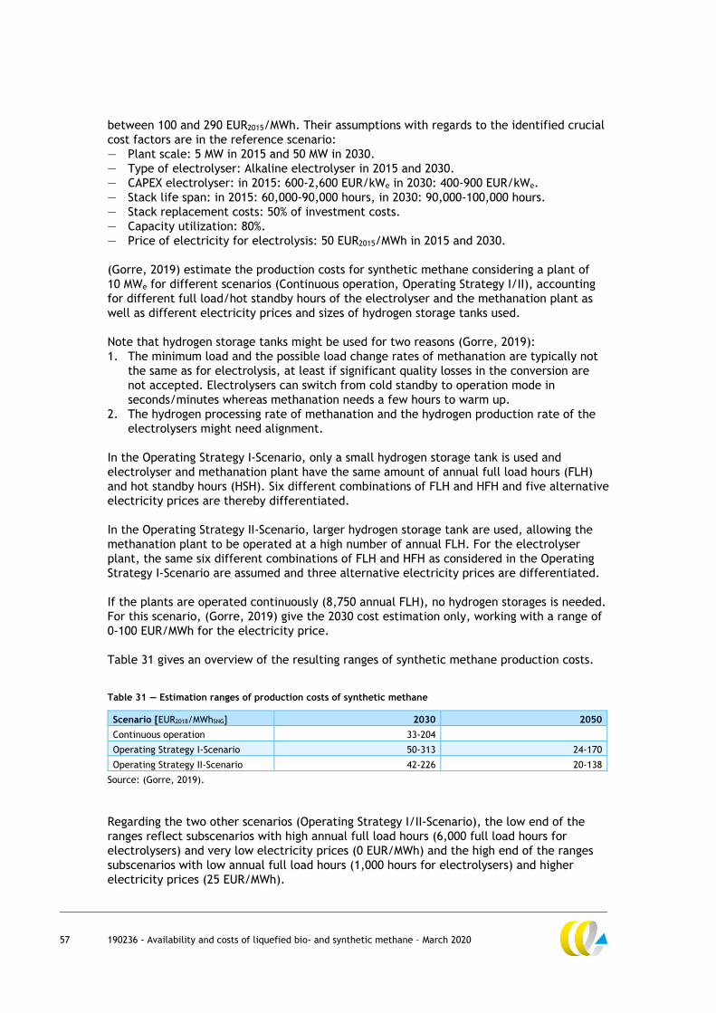
57 190236 - Availability and costs of liquefied bio- and synthetic methane – March 2020
between 100 and 290 EUR2015/MWh. Their assumptions with regards to the identified crucial
cost factors are in the reference scenario:
— Plant scale: 5 MW in 2015 and 50 MW in 2030.
— Type of electrolyser: Alkaline electrolyser in 2015 and 2030.
— CAPEX electrolyser: in 2015: 600-2,600 EUR/kWe in 2030: 400-900 EUR/kWe.
— Stack life span: in 2015: 60,000-90,000 hours, in 2030: 90,000-100,000 hours.
— Stack replacement costs: 50% of investment costs.
— Capacity utilization: 80%.
— Price of electricity for electrolysis: 50 EUR2015/MWh in 2015 and 2030.
(Gorre, 2019) estimate the production costs for synthetic methane considering a plant of
10 MWe for different scenarios (Continuous operation, Operating Strategy I/II), accounting
for different full load/hot standby hours of the electrolyser and the methanation plant as
well as different electricity prices and sizes of hydrogen storage tanks used.
Note that hydrogen storage tanks might be used for two reasons (Gorre, 2019):
1. The minimum load and the possible load change rates of methanation are typically not
the same as for electrolysis, at least if significant quality losses in the conversion are
not accepted. Electrolysers can switch from cold standby to operation mode in
seconds/minutes whereas methanation needs a few hours to warm up.
2. The hydrogen processing rate of methanation and the hydrogen production rate of the
electrolysers might need alignment.
In the Operating Strategy I-Scenario, only a small hydrogen storage tank is used and
electrolyser and methanation plant have the same amount of annual full load hours (FLH)
and hot standby hours (HSH). Six different combinations of FLH and HFH and five alternative
electricity prices are thereby differentiated.
In the Operating Strategy II-Scenario, larger hydrogen storage tank are used, allowing the
methanation plant to be operated at a high number of annual FLH. For the electrolyser
plant, the same six different combinations of FLH and HFH as considered in the Operating
Strategy I-Scenario are assumed and three alternative electricity prices are differentiated.
If the plants are operated continuously (8,750 annual FLH), no hydrogen storages is needed.
For this scenario, (Gorre, 2019) give the 2030 cost estimation only, working with a range of
0-100 EUR/MWh for the electricity price.
Table 31 gives an overview of the resulting ranges of synthetic methane production costs.
Table 31 — Estimation ranges of production costs of synthetic methane
Scenario [EUR2018/MWhSNG] 2030 2050
Continuous operation 33-204
Operating Strategy I-Scenario 50-313 24-170
Operating Strategy II-Scenario 42-226 20-138
Source: (Gorre, 2019).
Regarding the two other scenarios (Operating Strategy I/II-Scenario), the low end of the
ranges reflect subscenarios with high annual full load hours (6,000 full load hours for
electrolysers) and very low electricity prices (0 EUR/MWh) and the high end of the ranges
subscenarios with low annual full load hours (1,000 hours for electrolysers) and higher
electricity prices (25 EUR/MWh).

58 190236 - Availability and costs of liquefied bio- and synthetic methane – March 2020
For 2050, the production costs are estimated to be lower for each scenario mainly due to
the assumption that the costs of the main components (electrolyser, methanation reactor
and CO2 separation units) will decline due to technological learning.
Since 6,000 full load hours for electrolysers and an electricity price of 0 EUR/MWh might
not be feasible (and especially the combination thereof), we also give the cost ranges for
maximally 4,000 annual full load hours and an electricity price of 10/25 EUR/MWh as
derived by (Gorre, 2019):
Table 32 — Estimation ranges of production costs of synthetic methane (10 MWe plant, (sub)scenarios with
maximally 4,000 annual full load hours and two alternative electricity prices (10/25 EUR/MWh))
Scenario [EUR2018/MWhsynthetic methane ] 2030 2050
Operating Strategy I-Scenario 88-313 53-170
Operating Strategy II-Scenario 72-226 43-138
Source: (Gorre, 2019).
With regards to the crucial assumptions as established above, (Gorre, 2019) assume:
— Plant scale: detailed scenario for 10 MWe plant, but CAPEX also specified for 1 and
50 MWe plants.
— Type of electrolyser: not specified.
— CAPEX electrolyser: 2017: 1180 EUR2017/kWe; 2030: 415-665 EUR2017/kWe (50-1 MW
plant); 2050: 220-350 EUR2017/kWe (50-1 MW plant).
— Stack life span: 10 years.
— Stack replacement costs: not specifically reported for the stack.
— Capacity utilization scenarios:
Operation Strategy I: electrolysers and methanation plant are operated in the same
way: 1,000/2,000/4,000/6,000 full load hours with the remaining hours (to the
maximum annual operating hours of 8,760) in hot standby;
Operation Strategy II: electrolyser are operated just as under Operation Strategy I
and methanation plant is operated almost continuously (8,500 full load hours and
260 hours in hot standby).
— Price of electricity for electrolysis: different scenarios: 0/1/5/10/25 EUR2017/MWh.
(Frontier Economics, 2018) have estimated the 2030 and 2050 costs for producing different
synthetic fuels for four main scenarios. In the first scenario, synthetic fuel is produced in
Germany using North and Baltic Sea offshore wind power, in the second and third scenario it
is produced in North Africa and Middle East respectively, using PV/wind systems, and in the
fourth scenario, it is produced in Iceland using geothermal/hydropower. Their model, which
is available online20, allows to calculate the production costs of synthetic methane for each
of the four scenarios and for alternative inputs, like direct air capture (TSA)/CCU (cement
industry), low/base/high cost reduction in the future, different load hours per year, etc.
Table 33 gives the resulting cost ranges (reflecting the different scenarios) for direct air
capture of CO2 and carbon capture at cement plants assuming 8,000 full load hours per year
from geothermal/hydropower in Iceland and 4,000 full load hours from PV/wind systems in
the per year — annual full load hours estimated to be realistic by (Frontier Economics,
2018).
________________________________ 20 See Agora PtG/PtL Calculator
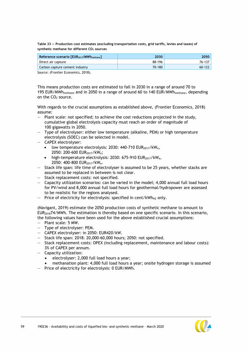
59 190236 - Availability and costs of liquefied bio- and synthetic methane – March 2020
Table 33 — Production cost estimates (excluding transportation costs, grid tariffs, levies and taxes) of
synthetic methane for different CO2 sources
Reference scenario [EUR2017/MWhmethane] 2030 2050
Direct air capture 88-196 76-137
Carbon capture cement industry 70-180 60-122
Source: (Frontier Economics, 2018).
This means production costs are estimated to fall in 2030 in a range of around 70 to
195 EUR/MWhmethane and in 2050 in a range of around 60 to 140 EUR/MWhmethane, depending
on the CO2 source.
With regards to the crucial assumptions as established above, (Frontier Economics, 2018)
assume:
— Plant scale: not specified; to achieve the cost reductions projected in the study,
cumulative global electrolysis capacity must reach an order of magnitude of
100 gigawatts in 2050.
— Type of electrolyser: either low temperature (alkaline, PEM) or high temperature
electrolysis (SOEC) can be selected in model.
— CAPEX electrolyser:
low temperature electrolysis: 2030: 440-710 EUR2017/kWe,
2050: 200-600 EUR2017/kWe;
high-temperature electrolysis: 2030: 675-910 EUR2017/kWe,
2050: 400-800 EUR2017/kWe.
— Stack life span: life time of electrolyser is assumed to be 25 years, whether stacks are
assumed to be replaced in between is not clear.
— Stack replacement costs: not specified.
— Capacity utilization scenarios: can be varied in the model; 4,000 annual full load hours
for PV/wind and 8,000 annual full load hours for geothermal/hydropower are assessed
to be realistic for the regions analysed.
— Price of electricity for electrolysis: specified in cent/kWhH2 only.
(Navigant, 2019) estimate the 2050 production costs of synthetic methane to amount to
EUR201874/MWh. The estimation is thereby based on one specific scenario. In this scenario,
the following values have been used for the above established crucial assumptions:
— Plant scale: 5 MW.
— Type of electrolyser: PEM.
— CAPEX electrolyser: in 2050: EUR420/kW.
— Stack life span: 2018: 20,000-60,000 hours; 2050: not specified.
— Stack replacement costs: OPEX (including replacement, maintenance and labour costs):
3% of CAPEX per annum.
— Capacity utilization:
electrolyser: 2,000 full load hours a year;
methanation plant: 4,000 full load hours a year; onsite hydrogen storage is assumed
— Price of electricity for electrolysis: 0 EUR/MWh.

60 190236 - Availability and costs of liquefied bio- and synthetic methane – March 2020
Conclusions
Our literature review confirms the findings of (Selma, et al., 2018) in the sense that we also
find varying estimates for the production costs of synthetic methane: for 2030 between
around 23-110 USD2019/MMBtu for 2050 and of around 15-60 USD2019/MMBtu.
These broad cost differences can be attributed to the different assumptions regarding the
size of the plant analysed, the operating hours of the plant and the electricity costs for
electrolysis. Optimization of the constellation and operation of the different parts of the
plants can also have a significant impact on the production costs. Using excess renewable
electricity can be expected to lead to relative low electricity costs for electrolysis (some
studies even assume that excess electricity is free), but will probably only allow for a small
number of operating hours per year and might require hydrogen storage or the methanation
plant to be on standby.
61 190236 - Availability and costs of liquefied bio- and synthetic methane – March 2020
4 Comparison of costs
4.1 Introduction
Next to LSM and LBM, there are several other types of zero/low fossil carbon bunker fuels
under discussion. Ship owners/operator will select a specific option, depending on the
availability and the according total cost of ownership. An analysis of the total cost of
ownership for different ship types/sizes and operational patterns, depending on the fuel
used and the according propulsion system is out of the scope of this study. What we do in
this chapter is to rather compare, first, the expected bunker cost price of LBM and LSM with
the expected bunker cost price of two fossil bunker fuels (LNG and VLSFO) and, second, we
compare the costs for LBM, LSM, liquid hydrogen and ammonia excluding transportation and
bunkering costs — the former being highly dependent on the production location and the
latter still being very uncertain for hydrogen and ammonia.
Since data availability for 2050 is rather poor, the comparison will focus on 2030.
A qualitative outlook will be given for the period between 2030 and 2050.
4.2 Production costs of synthetic and biomethane
We have conducted a literature review to determine the cost price of synthetic and
biomethane at plant (see Section 2.3.1 and Section 3.3.1):
For biomethane for the current situation, the cost price from anaerobic digestion is
estimated to lie in the range of around 20 to 50 USD/MMBtu and to be lower than for
gasification (around 25-65 USD/MMBtu). For both processes, production costs are expected
to be lower in 2050, with the costs for gasification (13 USD/MMBtu) then being lower than
for anaerobic digestion (15-21 USD/MMBtu). However, only limited research has been
carried out for the 2050 situation.
The estimations of the cost price of synthetic methane vary highly:
around 23-110 USD/MMBtu for 2030 and around 15-60 USD/MMBtu for 2050.
4.3 Production costs of hydrogen
Hydrogen produced by means of water electrolysis is one of the renewable fuel options
under discussion for maritime shipping. Hydrogen can be used in fuel cells. In principle, it
can also be used in internal combustion engines, but a marine internal combustion engine
has not been developed yet and, to our knowledge, is currently not under development.
Hydrogen has the advantage that it does require no/very little pre-treatment if used in fuel
cells and the production costs of hydrogen can be expected to be lower than the production
costs of synthetic methane since the production of hydrogen is part of the production of
synthetic methane.
But hydrogen has also got some disadvantages. It has a low volumetric energy density and a
very low boiling point (-253°C), requiring energy intensive liquefaction and cryogenic
storage for use and transport by ships. It is also extremely flammable and may explode if
heated.

62 190236 - Availability and costs of liquefied bio- and synthetic methane – March 2020
Several estimations of the production costs of renewable hydrogen can be found in the
literature. Table 40 in Annex D.2 provides an overview. Most estimations are related to
2030, but some studies also provide estimations for 2050. Estimations for production costs
of renewable hydrogen of between 10 and 63 USD/MMBtu for 2030 and between 5 and
25 USD/MMBtu for 2050 can be found in the literature.
4.4 Production costs of ammonia
Next to hydrogen, ammonia is discussed as a potential renewable fuel for maritime
shipping. Ammonia can potentially be use in internal combustion engines and, as a hydrogen
carrier, also in fuel cells. A marine internal combustion engine for ammonia is not available
yet, but the development time is estimated to amount to 2 to 3 years.
Ammonia is an important industrial product, the majority being used to produce fertilizer.
The Haber-Bosch process for the production of ammonia is a well-established process.
Atmospheric nitrogen and hydrogen, currently obtained from natural gas, are the main
inputs for this process. In order to produce renewable, carbon-free ammonia, the hydrogen
used as an input for the process would, just as for LSM, need to be produced by means of
water electrolysis. In contrast to the production of LSM, ammonia production does not
require CO2 capturing, but capturing of nitrogen. The advantage is that the concentration of
nitrogen in the atmosphere is relatively high and that the nitrogen capturing process is well
established.
Alternative ammonia synthesis technologies have been explored, like solid state ammonia
synthesis and biochemical solutions, but according to Cerulogy (2017) these technologies
will not be available at commercial scale the next 10 years and data availability for these
technologies is very poor.
When compared to LSM/LBM and hydrogen, ammonia has the advantage that its boiling
point is relatively high (around -33.40°C) which means that it can become liquid at relative
low pressure and does not require cryogenic storage. Liquefaction, storage and
transportation costs are therefore significantly lower. This is also why for the transport of
hydrogen its conversion to ammonia is discussed in the literature. In addition, it is
considered a flammable gas rather than an extremely flammable gas like methane.
The latter, together with a high auto ignition temperature, makes handling of ammonia
relatively safe, but is at the same time a challenge for the combustion process.
A major disadvantage of ammonia is however its toxicity: According to the harmonised
classification and labelling approved by the European Union, it causes severe skin burns and
eye damage, is toxic if inhaled and is also very toxic to aquatic life (ECHA, 2020).
In addition, ammonia is corrosive to copper, copper alloys, nickel and plastics (Brohi, 2014).
Different estimations of the production costs of renewable ammonia can be found in the
literature. Table 39 in Annex D.1 provides an according overview. Most of these studies
estimate the expected current costs and/or the expected costs in 2025/2030 and only one
study that we are aware of estimates the expected costs in 2050. The major differences
between the production cost estimations seem to be the price of the renewable electricity
assumed for the production of hydrogen and the assumed electrolyser load factors. The
former differs, depending on the assumed production location, the renewable energy source
and the expected future efficiency improvement of the according conversion technology.

63 190236 - Availability and costs of liquefied bio- and synthetic methane – March 2020
From the literature review we conclude that, the production cost of renewable ammonia is
estimated to lie in a range of 17 to 105 USD/MMBtu for 2025/2030 and one study estimates
the costs to be around 10 USD/MMBtu in 2050.
Given the fact, that the production of renewable ammonia uses renewable hydrogen as
input, production costs of renewable ammonia should inherently be higher than the
production costs of renewable hydrogen, at least, given the same hydrogen production
process and costs. Comparing the cost estimations for ammonia and hydrogen, this is only
reflected in the lower end of the cost range. This means that different assumptions have
been made with regards to hydrogen production in the estimations of the hydrogen and the
ammonia production costs, probably with regards to the production location and the
according electricity price.
4.5 Liquefaction, transport and bunker infrastructure costs of the alternative
fuels
4.5.1 LBM and LSM
Liquefaction, transportation and bunker infrastructure costs can be expected to be the
same for (L)BM and (L)SM as well as (L)NG at least if the production location is assumed to
be the same.
Liquefaction costs
Methane has a boiling point of -162°C which means that it has to be cooled down to -162°C
to become liquid. Liquefaction of methane is therefore an energy intensive process. Based
on the performance evaluation of real life liquefaction terminals, the energy demand of the
process is assessed to be up to 10% of the supplied natural gas (Pospisil & Charvat, 2019).
For the liquefaction of natural gas, DNV GL (2019b) finds 3 to 5 USD/MMBtu to be an
adequate cost range estimate for today (end of 2019) and OIES and University of Oxford
(2018) give liquefaction costs for different plants, ranging from 2.5 to 4.5 USD/MMBtu.
For the following analysis we assume the 2030 liquefaction costs to be at the lower range of
the current costs, i.e. to be 3 USD/MMBtu.
Transport costs
The transport costs considered in this study are the costs for transporting the methane to
the port, for fuelling of ships.
Independent of the fuel transported, transport costs will differ highly depending on the
location of the production and the location of the port where the bunker fuel will be sold.
There are two main options for the transport of the methane to a port:
1. Transport by pipeline, in gaseous form. The methane will in this case be liquefied in the
harbour and not at the plant:
a The gaseous methane is injected into the natural gas grid.
b An existing gas pipeline is prepared for use as dedicated pipeline.
c A new pipeline is built.
2. Transport by truck and/or ship, in liquid form. The methane will in these cases be
liquefied at the location of production.

64 190236 - Availability and costs of liquefied bio- and synthetic methane – March 2020
Transport by pipeline – injection into NG grid
When synthetic/biomethane is injected into the natural gas grid, this results in a mixture
with natural gas. Liquefaction systems in ports could then administratively produce
LSM/LBM, if they bought according certificates from the producer. In case of a dedicated
synthetic/biomethane pipeline, synthetic/biomethane is physically delivered to the port,
and the bunker fuel supplier will physically receive 100% synthetic/biomethane.
Transport by pipeline – use of existing gas pipeline
Not all biomethane production locations will be close enough to the harbour to make the
construction of a new pipeline a cost-effective option. However, in some cases it may be
possible to transform a former natural gas pipeline (or other pipeline) into a dedicated
biomethane pipeline. This will be much cheaper than building a new pipeline. Biomethane
has the same composition as natural gas, so the cost of preparing a natural gas pipeline is
limited to the cost of executing the isolation of the pipeline from the natural gas grid.
Compared to option 1a (injection into the natural gas grid), the pipeline preparation/
transformation cost is added to the biomethane production cost.
Transport by pipeline – realisation of new pipeline
Building a dedicated biomethane pipeline for a single biomethane plant will be expensive,
but if multiple biomethane plants can make use of the same (backbone) pipeline to the
harbour, the investment costs can be shared. The pipeline diameter will be larger in these
cases, which will reduce the material cost per kilometre. Baldino et al. (2018) indicate,
based on data from the New York State Energy R&D Authority, that the pipeline CAPEX of a
biogas pipeline for a single farm are 100,000-200,000 EUR per kilometre. Trinomics et al.
(2019) show higher values based on a literature review: a CAPEX of transmission pipelines
of400,000-1,500,000 EUR/km and a CAPEX of distribution pipelines of 300,000-900,000
EUR/km, with higher values representing larger pipeline diameters.
Under all options of pipeline transport, there are injection and connection costs associated
with the connection of the plant to the pipeline and feed-in of the methane. These include
the investment in injection capacity and operational expenses. Also, in all options, the
OPEX includes the costs of compression and measurement. Other costs, such as conditioning
of the methane to the gas quality in the grid and odorisation, are only applicable when the
biomethane is injected into the natural gas grid.
Economies of scale play a large role in the CAPEX of the injection system. As a result,
methane injection costs may decrease from 0.46-0.69 USD/m3 at 100 m3 gas/hour to
0.05-0.1 USD/m3 at 2,000 m3 gas/hour according to IRENA (2018b).These costs include
conditioning and odorisation costs, so for dedicated pipelines the values will be lower.
The difference between the minimum and maximum values mainly reflects the different
costs of biomethane compression, as injection into low-pressure grids is cheaper than
injection into high-pressure grids. The share of CAPEX in total grid injection costs drops
from more than 50% to less than 30% (IRENA, 2018b).
Navigant (2019) estimates grid injection cost of biomethane at 3.3 USD/MWh and
connection costs at 2.2 USD/MWh (assuming 1 km steel pipes).
Transport by truck
In cases where grid injection and pipeline modification are undesirable and/or not possible
(for example, due to the absence of a gas grid) and where the distance between the

65 190236 - Availability and costs of liquefied bio- and synthetic methane – March 2020
biomethane production location and the port is too large (in the order of more than
5-10 kilometres for small pipelines and more than 30-50 km for medium pipelines, according
to Vasilevich et al. (2016) transport of liquid methane by truck is the cheapest solution.
The cost of LNG transport by truck is estimated at 3.4-6.8 USD/MWh by Tractebel
Engineering (2015). Larger quantities and shorter transport distances lead to lower
transport costs. IRENA (2018b) reports costs of biomethane as a compressed gas
(in high-pressure steel cylinders on trucks) of 0.17-0.22 USD/m3.
Transport by ship
If liquefied at the production site, liquefied methane can also be transported by ship.
The according liquefied methane shipping costs are difficult to estimate, given the time
charter rates (USD/day per vessel) for LNG vessels have been very volatile in the past, as
illustrated in Figure 15.
Figure 15 — Historical LNG time charter rates
Source: Clarksons in (FT, 2018).
66 190236 - Availability and costs of liquefied bio- and synthetic methane – March 2020
Bunkering costs
LBM and LSM have the advantage that they can make use of LNG bunkering infrastructure
which is technically mature and commercially available.
Just as for LNG, there are in principle three different options for the bunkering of LBM and
LSM (website World Port Sustainability Program, 2019):
— Currently, truck-to-ship bunkering is used most often, because of limited demand from
ships, a lack of infrastructure and relatively low investment costs. A disadvantage of
this bunkering method is the limited capacity of trucks of approximately 40-80 m3.
Therefore, this method is not suitable for larger ships.
— Ship-to-ship bunkering can take place at various locations (even at sea) and is a
flexible bunkering method, but bunker vessels are costly and can hardly be used for
other commercial operations. It is expected that ship-to-ship bunkering becomes the
main bunkering method in the future, when a large fleet of LNG/LBM/LSM-fuelled ships
has developed.
— A third bunkering method is shore-to ship bunkering, in which case the liquefied
methane is delivered to the ship directly from a tank, station, or terminal. This method
is suitable for ports with a stable bunkering demand, but is less flexible and it takes
more effort for ships to get to the location.
For each of these methods it holds that the availability is still limited worldwide.
For ship-to-ship bunkering — the conventional bunkering method in maritime shipping —
LNG bunkering vessels are required. Currently (November 2019), eight LNG bunkering
vessels are in service worldwide, excluding LNG bunkering barges, and eight LNG bunkering
vessels are on order.
CE Delft and TNO (2015) have calculated the costs for LNG supply in different EU ports,
considering the value chain from the import terminal on. Alternative forms of LNG transport
between import terminal and port and alternative bunkering methods as well as local
specific factors (like distances and LNG sold per year), result in a cost range of 1 to
4 USD/MMBtu. If LNG supply in ports is scaled-up in the future, these costs can be expected
to decline.
4.5.2 Hydrogen
Hydrogen has a much higher energy density per unit of mass if compared to methane,
however it has a lower volumetric density which means that hydrogen requires more storage
space per unit of energy than methane. Hydrogen, just as methane, needs to be liquefied
for the use on board ships. With a boiling point lower than methane (-253°C vs -161°C)
liquefaction of hydrogen is more energy intensive than the liquefaction of methane.
According to IRENA (2019d), the amount of electricity that is required to liquefy hydrogen,
would currently lead to losses of 20 to 45% of the hydrogen energy content. According to
IEA (2019d) hydrogen liquefaction costs amount to around 1 USD/kg H2 (or 9 USD/MMBtu)
and is the value we apply in the cost comparison. The value falls in the range of the range
of the hydrogen liquefaction costs as given by (Lloyd's Register; UMAS, 2019): 0.5 and
1.1 €/kg H2 or 5-11 USD/MMBtu.
High storage and liquefaction costs makes transport of hydrogen by ships costly. This is why
for transportation purposes, conversion of hydrogen into other energy carriers, for example
ammonia, is an option discussed in the literature. According to IEA (2019d) “for distances
below 1,500 km, transporting hydrogen as a gas by pipeline is likely to be the cheapest
delivery option; above 1,500 km, shipping hydrogen as ammonia or an LOHC [liquid organic
hydrogen carrier] is likely to be more cost-effective.” When choosing a production location

67 190236 - Availability and costs of liquefied bio- and synthetic methane – March 2020
for renewable hydrogen, it will thus be important to find a balance between electricity
costs and transport distance.
Bunkering infrastructure for hydrogen is still under development: for land-based
transportation, there are refuelling stations for liquid hydrogen, but for maritime shipping
the infrastructure is technologically not mature yet (NCE Maritime Cleantech, 2019).
Different options are being discussed in this context and feasibility studies are carried out
(NCE Maritime Cleantech, 2019).
4.5.3 Ammonia
When compared to LSM/LBM, ammonia has the advantage that its boiling point is relatively
high (around -33.40°C) which means that it can become liquid at relative low pressure
and/or under relatively mild conditions. Liquefaction, storage and transport costs are
therefore lower than for hydrogen and LNG/LSM/LBM. The energy required for the
liquefaction of ammonia is expected to be relatively low — less than 0.1 percentage by mass
of ammonia — and can therefore be considered negligible.
Regarding the transportation costs of ammonia, not much information can be found in the
literature. According to (IEA, 2017c) ammonia could be shipped at a cost of 40 USD/t NH3 to
60 USD/t NH3 (which corresponds to 2.3-3.4 USD/MMBtu) depending on distance and vessel
size. CE Delft (2018b) assumes the transportation of ammonia from Morocco to the
Netherlands to cost 0.16 EUR/kg H2 (which corresponds to around 1.5 USD/MMBtu).
Bunkering infrastructure for ammonia has not been developed yet at all. Since ammonia is
shipped as cargo, it can be expected that the development of the infrastructure will be
able to build on the experience from ammonia handling, but there are no estimations of the
infrastructure costs in the literature available yet.
4.6 Fossil bunker fuels
4.6.1 Fossil bunker fuel prices
LNG
LNG bunker prices are only starting to be reported and LNG bunker price projections are
also scarce. Nevertheless, to come to an estimation of the 2030 LNG bunker price, the
following approach has been applied:
1. There are regional differences between natural gas prices. Currently, the natural gas
price in the US is lower than the natural gas price in Europe; in Japan, where natural
gas is imported as LNG, the natural gas price is highest. According to the World Bank
(2019) it can be expected that in 2030, the US and the Japanese natural gas price will
still represent the lower and higher end of the natural gas price range.
2. Based on the World Bank Commodities Price Forecast (World Bank, 2019) for US natural
gas and for LNG in Japan in 2030, we estimate an according 2030 LNG bunker fuel price
range.
According to the World Bank Commodities Price Forecast (World Bank, 2019), the US
natural gas price is expected to amount to 4 USD/MMBtu and the Japanese LNG price to
8.5 USD/MMBtu. Applying the methodology as presented in SEA\LNG (2019), i.e. adding
liquefaction costs and specific mark-ups to the US natural gas price, a 2030 LNG bunkering

68 190236 - Availability and costs of liquefied bio- and synthetic methane – March 2020
price of around 11 USD/MMBtu is estimated as the lower range. Assuming that the
LNG logistics and bunkering costs in Japan are comparable to the costs in the US
(3.08 USD/MMBtu as specified in SEA\LNG (SEA\LNG, 2019)), we estimate a 2030 LNG
bunkering price of around 12 USD/MMBtu as the higher range.
As a result we work with a 2030 LNG bunker price range of 11-12 USD/MMBtu.
Very Low Sulphur Fuel Oil (VLSFO)
Since beginning of 2020, maritime ships are obliged to use fuel with a maximum sulphur
content of 0.5% m/m if sailing outside Emission Control Areas. Ships also use exhaust gas
cleaning systems to comply with the regulation, but so far, the majority of the ships use
VLSFO to comply the sulphur regulation; a small, but increasing share of ships use LNG.
Since there are very little historical data on VLSFO prices available, no valid correlations
with for example the crude oil price can be established, making an estimation of the 2030
VLSFO price even more difficult than the estimation of the 2030 LNG price. To nevertheless
come to an estimation of the 2030 VLSFO bunker price, the following approach has been
applied:
1. We have determined a range of the average VLSFO price for the period 1 November
2019–27 January 2020, with the average price in Rotterdam representing the lower and
the average price in Singapore the higher end of the range. Publicly available data from
Ship & Bunker (2019) have been used to this end. This resulted in a range of 531–
621 USD/mt21 which is equivalent to 14-15.7 USD/MMBtu.
2. We have compared the average crude oil price for the same period and compared it
with the 2030 World Bank crude oil price estimation (70 USD/barrel) to establish the
potential maximum increase of the VLSFO price until 2030. This resulted in a potential
maximum increase of around 8%.
3. Applying this maximum increase to the bunker price range as established under point 1,
this results in a 2030 VLSFO bunker price range of around 15-17 USD/MMBtu.
4.6.2 Carbon mark-up
In its Initial Strategy on Reduction of GHG emissions from ships (MEPC.304(72)), the IMO has
agreed on a level of ambition and on the development of policy measures to meet this level
of ambition. However, no specific measures and thus also no specific stringency levels of
have been agreed upon yet. This makes it difficult to estimate the carbon price that will
become effective for the maritime shipping sector.
The IMO aims to phase out GHG emissions from international shipping as soon as possible in
this century and perceives its 2050 goal (50% by 2050 compared to 2008) as a point on a
pathway of CO2 emissions reduction consistent with the Paris Agreement temperature goals.
We therefore decided to use a carbon prices in line with estimations of the global average
carbon prices required to implement the Paris Agreement temperature goals.
There are different estimations of average regional, but only very few estimations of global
average carbon prices required to implement the Paris Agreement temperature goals.
________________________________ 21 Please be aware that the VLSFO featured a price spike beginning of January 2020 which in retrospective could
turn out to be an outlier, but at this point in time this is still unclear.

69 190236 - Availability and costs of liquefied bio- and synthetic methane – March 2020
The High-Level Commission on Carbon Prices (2017) concludes that the carbon-price level
consistent with achieving the Paris temperature target (increase of well below 2°C above
pre-industrial levels) is at least 40–80 USD/t CO2 by 2020 and 50–100 USD/t CO2 by 2030,
provided a supportive policy environment is in place.
For the cost price comparison of the different bunker fuels we therefore stick to the 2030
carbon price range of 50–100 USD/t CO2. This translates into the following carbon price
mark-up per MMBtu:
— LNG: 3.0-6.1 USD/MMBtu;
— VLSFO: 4.0–8.0 USD/MMBtu.
For the conversion of the carbon price mark-up, the following assumptions have been made,
based on the EEDI guidelines (MEPC 73/19/Add.1, Annex 5):
— CO2 emission factors: 2.75 kg CO2/kg LNG, 3.114 kg CO2/kg HFO, and 3.206 CO2/kg MGO;
— Lower heating values of the fuels: 48 MJ/kg LNG, 40.2 MJ/kg HFO, and 42.7 MJ/kg MGO;
— VLSFO is assumed to be a blend consisting of 20% HFO and 80% MGO.
4.6.3 Fossil bunker fuels including carbon mark-up
Combining the 2030 price estimations for LNG and VLSFO excluding a carbon price (see
Section 4.6.1) and the carbon mark-up as derived under 4.6.2, we estimate the 2030 bunker
prices of LNG and VLSFO including a carbon price of 50–100 USD/tCO2 to be around:
— 14-18 USD/MMBtu for LNG; and
— 19-25 USD/MMBtu for VLSFO.
4.7 Cost comparison
Data availability allows for a limited comparison of the different bunker fuels only.
In the following we will present two different cost comparisons:
1. First, we compare the expected bunker prices for the fossil bunker fuels (LNG & VLSFO)
with the expected bunker costs for LBM and LSM. For LBM and LSM we thereby assume
the same liquefaction, distribution and bunkering costs as for NG. No long-distance
transportation costs for LBM and LSM since these highly depend on the production
location. This implicitly implies that LBM and LSM are produced locally.
2. Second, we compare the costs for LBM, LSM, liquid hydrogen and ammonia excluding
transportation and bunkering costs — the former being highly dependent on the
production location and the latter still being very uncertain for hydrogen and ammonia.
As already indicated, data availability for 2050 is rather poor, which is why the comparison
will focus on 2030. For biomethane data for 2030 is not available: most cost data is related
to current costs and only a few studies have looked into 2050 costs. The 2030 cost estimates
for biomethane used in the following comparisons have therefore been derived by a rough
interpolation of the data available.
4.7.1 Comparison of fossil and renewable fuels
Table 34 presents estimations for the 2030 bunker prices of VLSFO, fossil LNG, LBM and LSM.
The bunker prices for VLSFO and fossil LNG include a carbon mark-up. For the estimation of
the bunker prices of fossil LNG, LBM and LSM, the same liquefaction costs (3 USD/MMBtu)
and the same LNG logistics and bunker costs (3 USD/MMBtu) and the same price mark-ups as
presented in SEA\LNG (2019) have been applied.

70 190236 - Availability and costs of liquefied bio- and synthetic methane – March 2020
Table 34 — Estimated 2030 per energy unit bunker prices for LBM and LSM compared with existing bunker
fuels
Bunker fuel Estimated 2030 bunker price (USD/MMBtu)
VLSFO 19-25 (including carbon mark-up)
Fossil LNG 14–18 (including carbon mark-up)
LBM 29-63
LSM 35-145
Per energy unit, fossil LNG is forecast to be the cheapest and LSM the most expensive
bunker fuel in 2030. Fossil LNG is estimated to be between 1 to 11 USD/MMBtu cheaper than
VLSFO. LSM can only be cheaper than LBM, if cheap renewable electricity is available and
high electrolyser load factors can be achieved.
From these estimations it can be concluded that a carbon mark-up of between 50–100 USD/t
CO2 will not be sufficient to incentivize a switch from fossil LNG to LBM or LSM in 2030.
Assuming that the bunker price of fossil LNG is constant after 2030 and that the lower range
of the 2030 production costs for LBM is relevant in the long-run, then a carbon mark-up of
around 280-300 USD/t CO2 would be required for LBM to become as expensive as fossil LNG.
According to the IPCC (2018) a 2050 carbon price of between 300 and 400 USD/t CO2 would
be consistent with a well below 2°C mitigation pathway.
4.7.2 Comparison of alternative renewable fuels
Comparing the 2030 per energy unit costs of LBM, LSM, liquid hydrogen and liquid ammonia,
excluding transportation and bunkering costs (Table 35), we find that
— The cost price range for LSM and liquid ammonia are rather broad, probably reflecting
the relative high uncertainty as well as a broad range of assumptions regarding the
electricity prices.
— The variation of the cost prices is lower at the lower range of the estimates.
— In an optimistic scenario (lower range of the cost estimates from the literature review),
• Plant gate costs are broadly comparable for LBM, liquid ammonia and liquid
hydrogen;
• At plant gate costs of liquid ammonia are expected to be lowest, followed by the
liquid hydrogen and LBM with LSM featuring the highest costs. Significantly lower
liquefaction costs for ammonia can explain the cost differential between liquid
ammonia and liquid hydrogen, but the presumed optimistic electricity price might
also vary between the estimates.
— In a pessimistic scenario (higher range of cost estimates), at plant gate costs of LBM are
expected to be lowest, followed by liquid hydrogen; costs for both, liquid ammonia and
LSM are relatively high and highest for LSM.
Table 35 — 2030 plant gate cost price estimates for different renewable bunker fuels
Cost price at plant gate (USD/MMBtu)
LBM 21-48
LSM 26-113
Liquid hydrogen 19-72
Liquid ammonia 17-105

71 190236 - Availability and costs of liquefied bio- and synthetic methane – March 2020
The optimistic cost estimates for liquid hydrogen, liquid ammonia and LSM can probably
only be achieved if the production location has favourable conditions for renewable
electricity. This may require the transportation of the fuels over longer distances,
depending on the locations of the bunker ports.
If transported by ship, transportation costs can be expected to be lower for liquid ammonia
compared to liquid hydrogen and LSM and indeed, LBM: due to its relatively high boiling
point it can become liquid at relative low pressure and/or under relatively mild conditions.
Liquefaction, storage and transport costs are therefore lower than for hydrogen and
LSM/LBM; for liquid hydrogen these costs can be expected to be higher than for LSM/LBM.
Since the production of LBM does not rely on the availability of cheap renewable electricity,
this might allow for local production in the vicinity of major ports and could save out costs
for the transport of the bunker fuel. Local production of LBM might require transport of
biomass. These transport costs can be expected to be relatively low, at least if the biomass
can be transported/is available in bulk.
Since the costs of the bunker infrastructure for hydrogen and ammonia are still very
uncertain, the impact of these costs on the bunker fuel prices are difficult to assess at
present. However, since the bunkering infrastructure of LBM and LSM are technically
mature whereas the bunkering infrastructure for hydrogen and ammonia is technically still
immature, the bunker price cost mark-up for the bunkering of hydrogen and ammonia can
be expected to be higher than for LSM and LBM, at least in the short- and medium-run.
72 190236 - Availability and costs of liquefied bio- and synthetic methane – March 2020
5 Discussion of availability for and
demand of shipping sector
The analysis of the availability of LBM (see Chapter 2) has focussed on the maximum
conceivable supply of LBM and the analysis of the availability of LSM (see Chapter 3) on the
renewable electricity required to supply the entire shipping sector with LSM.
It would however be unrealistic to assume that these volumes of LBM/LSM would actually all
become available to the shipping sector. Other sectors might switch from natural gas to LSM
or LBM too and the supply of LBM/LSM could be significantly lower, since the supply of the
fuels also depends on suppliers’ potential profit which in turn depends on the cost price of
the fuels, the consumers’ willingness to pay for the fuels and the potential volume of the
demand.
Biomass that can be used for the production of LBM could therefore be used in an
alternative way, i.e. either used directly or for the production of other gaseous or liquid
biofuels. And hydrogen and renewable electricity used for the production of LSM could also
be used in an alternative way, i.e. either used directly or for the production of other
synthetic gaseous or liquid fuels.
There are some feedstocks for which digestion and thus the production of biomethane is
one of the obvious choices: feedstocks with a high water content and a low sugar, oil or
starch content. But the majority of biomass feedstocks can be converted with different
technologies to produce different gaseous or liquid biofuels and other bio-based products.
Obvious potential buyer of LBM and LSM are sectors that, at the outset of the energy
transition, are using fossil (L)NG. By switching to LSM/LBM these sectors would avoid extra
costs for system adjustments and additional indirect costs for new supply infrastructure.
As Figure 16 shows, natural gas is currently mainly used in the power sector and for
(process) heating in the industry and in the built environment. In different industrial sectors
natural gas is also used as feedstock to produce hydrogen and chemicals. To a relatively
small extent, natural gas is used in the transport sector.

73 190236 - Availability and costs of liquefied bio- and synthetic methane – March 2020
Figure 16 — 2017 global gas consumption by sector
Source: BP Energy Outlook 2019.
For each of these sectors, we will analyse whether the current demand for (L)NG will
transform in demand for LSM or LBM in a decarbonized future, or that other fuels or energy
sources are more obvious candidates to replace (L)NG. Figure 17 illustrates this analysis.
The power sector currently uses (L)NG, amongst others, to produce electricity. Since LSM
requires the use of renewable electricity, and since there are energy losses in the
production of H2 from renewable electricity and again energy losses in the production of
LSM from H2 and other inputs, it does not make sense for the power sector to shift to LSM:
it would make more sense to sell renewable electricity directly or to store it as H2 and
convert H2 into electricity in a power plant rather than converting it into CH4 first.
It could be possible that the power sector would use (L)BM, although current and projected
levelized costs of wind- and solar power (see Annex C) are well below the production costs
of (L)BM, so it is unlikely that the power sector will use significant amounts of (L)BM in the
long run.
Another reason why the power sector could continue the use of biomass is to generate
negative emissions. Generating electricity with biomass, sequestering the CO2 emissions and
storing them would be one way to reduce the concentration of CO2 in the atmosphere. Such
negative emissions are a prevalent feature of emission scenarios consistent with the Paris
Agreement temperature goals (IPCC, 2018).
Industry uses (L)NG to produce electricity or heat and/or uses it as a feedstock (‘non
combusted’ in Figure 16). For the production of electricity or heat, it is unlikely that there
will be significant demand for LSM or LBM for the same reasons as apply to the power
sector.
(L)NG is a feedstock for the production of hydrogen. Since LSM is produced from hydrogen,
we don’t expect demand for LSM to feed into this production process.
For other feedstock use, the industry may have a significant demand for LSM and LBM to
replace natural gas in a decarbonised future.

74 190236 - Availability and costs of liquefied bio- and synthetic methane – March 2020
The built environment uses (L)NG for heating and cooking. In principle, buildings can
switch to other energy sources (electricity and heat pumps; hydrogen; liquid or solid
biomass), but such conversion might require considerable collective investments in
infrastructure and equipment which may be difficult to achieve, which is why there may be
demand for (L)BM and (L)SM from buildings.
The use of (L)NG in the transport sector is currently low, but a shift from liquid fuels to
gaseous fuels is conceivable for HGVs, inland vessels and non-road mobile machinery,
although electrification and the use of H2 are also possibilities. Note that LSM has an
advantage over synthetic liquid hydrocarbons because methane can be produced more
efficiently. Still, these sectors may also have a demand for LSM and LBM in a decarbonised
future.
Owners of LNG-fuelled ships that want to switch to LSM/LBM might thus have to compete
with the industry, the built environment and other transport sectors for LSM/LBM.

Figure 17 — Illustration of potential substitution of (L)NG by LSM/LBM in a decarbonised world

76 190236 - Availability and costs of liquefied bio- and synthetic methane – March 2020
6 Recommendations on how
barriers to scaling of LBM and LSM
as marine fuel could be addressed
Chapters 2 and 3 demonstrate that sufficient amounts of biomethane or synthetic methane
or a combination of these can be produced to fuel the entire shipping sector. Chapter 4
shows that carbon prices of USD 50–100 per tonne CO2 will not be sufficient to make either
biomethane or synthetic methane cost-competitive with fossil marine fuels. Chapter 5
concludes that in a decarbonized future, there will be competing demand for biomethane
and synthetic methane from other sectors, such as land transport, the built environment
and potentially industry.
This chapter addresses the question how barriers to scaling of LBM and LSM as marine fuel
could be addressed. It first identifies the main barriers as well as the factors that are
conducive to the uptake of LSM and LBM. Subsequently, it discusses how each of the
barriers could be addressed, taking the conducive factors into account.
6.1 Barriers and conducive factors
The main barriers are the high price of LSM and LBM relative to other marine fuels; the
relatively small (but growing) number of LNG ships in the current fleet; uncertainty about
the climate impacts of LNG, LSM and LBM, in particular relating to methane slip and the
climate impact of methane; and the fact that competing demand may come from sectors
that are accustomed to blending mandates and to higher fuel prices.
Counter to the barriers, there are also factors that could contribute to scaling of LBM and
LSM as marine fuel. One is that these are drop-in fuels and can be used by LNG-powered
ships without modifications to the engine or the fuel system. They can also be mixed in all
proportions with fossil LNG, thus creating a fuel with a specific net-carbon impact. Some of
these factors are related to methane in general, regardless of whether it is fossil, synthetic
or of a biological origin. The number of LNG-powered ships is increasing, amongst others
due to tighter air-quality regulations. And finally, the number of ports offering LNG
bunkering facilities is increasing rapidly in different parts of the world.
6.2 Measures in the shipping sector
We distinguish measures that can be taken in the shipping sector and measures in other
sectors.
The shipping sector could take measures to enhance the demand for methane-powered
ships in general and also measures that will increase demand specifically for the net-low-
and net-zero-carbon varieties of methane.

77 190236 - Availability and costs of liquefied bio- and synthetic methane – March 2020
The first category of measures comprises measures that reduce uncertainty about LNG as a
marine fuel. These uncertainties relate to price, bunkering infrastructure and the climate
impacts of methane.
Many of the first type of measures are already implemented. Standards, procedures and
safety regulations have been developed in the last few years which is why we do not see
any major institutional barriers to the use of LSM or LBM in shipping. ISO is currently also
developing the ‘Specification of liquefied natural gas as a fuel for marine applications’
(ISO/DIS 23306). This should allow to get a better understanding of the quality of LBM that
is required for use as marine fuel or for a blend of LNG and LBM or LSM as marine fuel.
The EU and other world regions are increasing the bunkering infrastructure. LNG provides
have various pricing options that alleviate some price risks.
MEPC is currently debating the carbon-emission factors of low- and zero-carbon fuels.
There is a debate about whether well-to-propeller or tank-to-propeller emission factors
should be used as a basis for future policy making. The climate impact of fuels is
determined by the well-to-propeller emissions. LSM and LBM have worse tank-to-propeller
emission factors than other low- or zero-carbon fuels like hydrogen or ammonia, which do
not contain carbon. In addition, there remains uncertainty about the methane slip of
bunkering, fuel systems and engines. The discussion would be helped with more empirical
data of methane slip in real-world conditions.
These measures address, combined or in isolation, the barrier of the relatively small but
increasing number of LNG-fuelled ships.
Specifically to increase demand for LSM and LBM from the shipping sector, measures would
have to be adopted that increase demand for low- or zero-carbon fuels or energy carriers at
the expense of fossil fuels. Obvious candidate measures would be a carbon levy, emissions
trading or fuel standard. A carbon levy would need to be higher than USD 100 per tonne of
CO2 in 2030 in order to make LSM and LBM cost-competitive. Emissions trading could have a
gradually lower cap so that allowance prices rise gradually to the required price level, and
a gradually increasing amount of LSM and LBM would be required by the shipping sector.
Likewise, a low-carbon fuel standard could mandate that ships gradually lower the average
fossil carbon content of the fuels used.
This measure could address the barriers of the relatively high cost of LSM and LBM
compared to other marine fuels, and the barrier that other sectors are already accustomed
to blending mandates and to higher fuel prices.
6.3 Measures in other sectors
Although the potential supply of LSM and LBM is high, the actual supply is very low.
Measures could be taken to enhance supply. Such measures can enhance supply directly or
be aimed at creating demand in other sectors which will trigger supply.
Supply could be enhanced by fostering R&D that brings down the production costs of LBM
and LSM
Regarding the supply side of LBM/LSM, there has to be sufficient overall demand for
suppliers to have an incentive to produce LSM/LBM. This is comparable to the current
situation – the marine sector would probably not have been able to use marine LNG if the
demand of other sectors for natural gas had not lead to the establishment of LNG markets.

78 190236 - Availability and costs of liquefied bio- and synthetic methane – March 2020
7 Conclusions
The aims of this study were to:
1. To assess the availability of LBM and LSM in relation to the global energy demand of
maritime shipping.
2. To assess the cost price of LBM and LSM and to compare it with the cost (price) of other
existing and potential marine bunker fuels.
3. To give recommendations as to how industry and policy makers could address barriers to
the scaling of LBM and LSM as a marine fuel.
Conclusions for each of these subjects are presented below.
7.1 Availability of LBM and LSM
LBM can be produced from energy crops, agricultural residues, forestry products and
revenues and from aquatic biomass. This study only takes biomass into account that can be
produced in a sustainable manner. The feedstocks can be converted into biomethane either
by anaerobic digestion, an established technology, or by gasification, which is being
developed. The maximum conceivable sustainable supply of LBM is calculated by assuming
that all sustainable biomass is converted into biomethane and subsequently liquefied.
Figure 18 compares the maximum conceivable sustainable supply of LBM with the projected
energy demand from the maritime sector in 2030 and 2050. In both years, the maximum
conceivable supply is larger than the demand from the maritime sector. Note however that
this analysis does not take into account that the actual production of biomass may be less
than the maximum conceivable production, that not all biomass will be converted into
methane and that there is competing demand from other sectors for methane.
Figure 18 — Maritime energy demand and global maximum sustainable supply of LBM in 2030 and 2050,
without aquatic biomass (EJ)

79 190236 - Availability and costs of liquefied bio- and synthetic methane – March 2020
The production of synthetic methane is not limited by land availability in the same way as
the production of biomethane is, because it doesn’t require arable land. Therefore, the
focus on the availability analysis is not on land availability and associated production
capacity, but rather on the availability of the scarcest input in the production process:
renewable electricity (all other inputs — hydrogen, fresh water, and carbon dioxide — are
produced with renewable electricity). While the potential capacity of renewable electricity
is very large, in practice it is constrained by the amount of investments.
Figure 19 shows the energy demand from maritime transport and the amount of renewable
electricity that would be required to meet this demand with LSM. Because of projected
improvements in the production process, the renewable electricity demand will decrease
when the projected energy demand increases. The amount of renewable electricity
required to produce LSM for the maritime sector is compared with the projected amount of
renewable electricity that will be required to limit global warming to 2 degrees above pre-
industrial levels. In 2050, an estimated 25-30% of renewable electricity would need to be
produced in addition to the projected amount to decarbonise the maritime transport sector
using LSM.
Figure 19 — Maximum potential supply of LSM compared with maritime energy demand given a renewable
electricity supply in line with a 2°C degree scenario
0
20
40
60
80
100
120
140
160
180
2015 2030 2050
EJ
Maritime energy demand
Required renewable electricity to power maritime shipping with LSM using available productiontechnologies
Available renewable electricity (2°C scenarios)

80 190236 - Availability and costs of liquefied bio- and synthetic methane – March 2020
7.2 Cost comparison
Comparing the expected 2030 per energy unit bunker prices of LBM, LSM and fossil LNG
(including a carbon mark-up), fossil LNG is forecast to be the cheapest and LSM the most
expensive bunker fuel in 2030. LSM can only become cheaper than LBM, if cheap renewable
electricity is available and high electrolyser load factors can be achieved. A carbon mark-up
of between 50–100 USD/t CO2 is not expected to be sufficient to incentivize a switch from
fossil LNG to LBM or LSM in 2030. However, a 2050 carbon price that is consistent with a
well below 2°C mitigation pathway can be expected to incentivize a switch from fossil LNG
to LBM, at least if the 2050 price for fossil LNG is not below its 2030 price.
Comparing plant gate costs of LBM and LSM with those of liquid hydrogen and liquid
ammonia — two other renewable fuels — it can be concluded that:
— In an optimistic scenario (lower range of the cost estimates from the literature review),
• Plant gate costs are broadly comparable for LBM, liquid ammonia and liquid
hydrogen.
• The costs of liquid ammonia are expected to be lowest, followed by the liquid
hydrogen and LBM with LSM featuring the highest costs. Significantly lower
liquefaction costs for ammonia can explain the cost differential between liquid
ammonia and liquid hydrogen, but the presumed optimistic electricity price might
also vary between the estimates.
— In a pessimistic scenario (higher range of cost estimates from the literature review), the
costs of LBM are expected to be lowest, followed by liquid hydrogen; costs for both,
liquid ammonia and LSM are relatively high and highest for LSM.
The optimistic scenario will probably only materialise for liquid hydrogen, liquid ammonia
and LSM if the production location has favourable conditions for renewable electricity.
This may require transportation of the fuels over longer distances, depending on the
locations of the bunker ports.
If transported by ship, transportation costs can be expected to be lower for liquid ammonia
compared to liquid hydrogen and LSM/LBM and for liquid hydrogen transportation costs can
be expected to be higher than for LSM/LBM.
Since the production of LBM does not rely on the availability of cheap renewable electricity,
this might allow for local production in the vicinity of major ports and could save out costs
for the transport of the bunker fuel. Local production of LBM might require transport of
biomass. These transport costs can be expected to be relatively low, at least if the biomass
can be transported/is available in bulk.
Since the costs of the bunker infrastructure for hydrogen and ammonia are still very
uncertain, the impact of these costs on the bunker fuel prices are difficult to assess at
present. However, since the bunkering infrastructure of LBM and LSM are technically
mature whereas the bunkering infrastructure for hydrogen and ammonia is technically still
immature, the bunker price cost mark-up for the bunkering of hydrogen and ammonia can
be expected to be higher than for LSM and LBM, at least in the short- and medium-run.
7.3 Recommendations for scaling up the use of LBM and LSM
In order to scale up the use of LSM and LBM, we recommend reducing the uncertainty about
the use of methane as a fuel, especially with regards to methane slip and the associated
climate impact. Policy measures like a fossil carbon levy, emissions trading or a low-carbon

81 190236 - Availability and costs of liquefied bio- and synthetic methane – March 2020
fuel standard could be implemented to shift the demand in the shipping sector from natural
gas or liquid fossil fuels to LSM, LBM or other low- and zero-carbon fuels.

82 190236 - Availability and costs of liquefied bio- and synthetic methane – March 2020
8 Literature
ABN AMRO, 2017. Energy Monitor – Renewable energy in Latin America. [Online]
Available at: https://insights.abnamro.nl/en/2018/05/energy-monitor-renewable-energy-
in-latin-america/
[Accessed 13 Sep 2019].
Adelung, S. & Kurkela, E., 2018. Flexible combined production of power, heat and
transport fuels from renewable energy sources, s.l.: DLR.
Baldino, C., Pavlenko, N., Searle, S. & Christensen, A., 2018. The potential for low-carbon
renewable methane as a transport fuel in France, Italy, and Spain. Working Paper , s.l.:
The International Council of Clean Transportation (ICCT).
Billig, E., 2016. Bewertung technischer und wirtschaftlicher Entwicklungspotenziale
künftiger und bestehender Biomass-zu-Methan-Koversionsprozesse, Leipzig: Universität
Leipzig.
BIOSURF, 2016. Technical-economic analysis for determining the feasibility threshold for
tradable biomethane certificates, D3.4 , s.l.: Istituto di Studi per L’Integrazione dei Sistemi
Scrl (ISINNOVA).
Blanco, H., Nijs, W. & Ruf, J., 2018. Potential of Power-to-Methane in the EU energy
transition to a low carbon system using cost optimization, s.l.: s.n.
Brohi, E. A., 2014. Ammonia as fuel for internal combustion engines? : An evaluation of the
feasibility of using nitrogen-based fuels in ICE, Gothenburg: Department of Applied
Mechanics, Chalmers University of Technology.
CCC, 2018. Biomass in a low-carbon economy, London: Committee on Climate Change
(CCC).
CE Delft ; TNO, 2015. Study on the Completion of an EU Framework on LNG-fuelled Ships
and its Relevant Fuel Provision Infrastructure - Lot 3 - Analysis of the LNG market
development in the EU, report for the European Commission, revised 2017, Delft: CE Delft.
CE Delft, Eclareon, Wageningen Research, 2016. Optimal use of biogas from waste streams:
an assessment of the potential of biogas from digestion in the EU beyond 2020, Brussels:
European Commission.
CE Delft, 2018a. Reduction of GHG emissions from ships, Delft: CE Delft.
CE Delft, 2018b. Waterstofroutes Nederland : Blauw, groen en import, Delft: CE Delft.
CE Delft, 2018c. Verkenning BioLNG voor transport : Fact finding, marktverkenning,
businesscases, Delft: CE Delft.
CE Delft, 2019. CO2-balansen groengasketens: Vergisting en vergassing, Delft: CE Delft.
Cedigaz, 2019. Global biomethane market: green gas goes global, press release. [Online]
Available at: https://www.cedigaz.org/global-biomethane-market-green-gas-goes-global/
[Accessed 2020].
Cerulogy, 2017. What role is there for electrofuel technologies in european transport's low
carbon future, s.l.: T&E.
Clean energy council, 2019. Clean energy australia report, s.l.: Clean energy council.

83 190236 - Availability and costs of liquefied bio- and synthetic methane – March 2020
Creutzig, F. et al., 2015. Bioenergy and climate change mitigation: an assessment. GCB
Bioenergy, 7(5), pp. 916-944.
Cucchiella, F., D’Adamo, I. & Gastaldi, M., 2015. Profitability analysis for biomethane: a
strategic role in the italian transport sector. International Journal of Energy Economics and
Policy, 5(2), pp. 440-449.
Daioglou, V. et al., 2019. Integrated assessment of biomass supply and demand in climate
change mitigation scenarios. Global environmental change, Volume 54, pp. 88-101.
Dibenedetto, A., 2011. The potential of aquatic biomass for CO2‐enhanced fixation and
energy production. Greenhouse Gases: Science and Technology, 1(1), pp. 58-71.
DNV GL, 2019a. Maritime Forecast to 2050 - Energy transistion outlook 2019, Oslo: DNV GL.
DNV-GL, 2019b. Current price development oil and gas. [Online]
Available at: https://www.dnvgl.com/maritime/lng/current-price-development-oil-and-
gas.html
[Accessed 2019].
E&E, 2014. Study on Hydrogen and methanation as means. Lyon, s.n.
E4tech, 2014. Study on development of water electrolysis in the EU, s.l.: E4tech.
EA Energianalyse ; SDU , 2016. Biogas Og Andre VE Braendstoffer Til Tung Transport,
København K: Ea Energianalyse a/s .
ECHA, 2020. Substance Infocard : Ammonia, anhydrous, Helsinki: European Chemicals
Agency (ECHA).
Ecofys, 2008. Worldwide potential of aquatic biomass.
Ecofys, 2018. Gas for Climate : How gas can help to achieve the Paris Agreement target in
an affordable way, Utrecht: Ecofys.
ET energy world , 2019. India’s largest renewable energy companies: Acme, Adani and
Greenko top the list. [Online]
Available at: https://energy.economictimes.indiatimes.com/news/renewable/indias-
largest-renewable-energy-companies-acme-adani-and-greenko-top-the-list/70429534
[Accessed 13 Sep 2019].
EU, 2018. Directive (EU) 2018/2001 of the European Parliament and of the Council of 11
December 2018 on the promotion of the use of energy from renewable sources. Offcial
Jorunal of the European Union, L328(21.12.2018), pp. 82-209.
Eurostat, 2017. Wind power becomes the most important renewable source of electricity.
[Online]
Available at: https://ec.europa.eu/eurostat/statistics-
explained/index.php/Renewable_energy_statistics#Wind_power_becomes_the_most_import
ant_renewable_source_of_electricity
[Accessed 13 Sep 2019].
Froehlich, H. E., Afflerbach, J. C., Frazier, M. & Halpern, B. S., 2019. Blue growth potential
to mitigate climate change through seaweed offsetting. Current Biology, 29(18), pp. 3087-
3093.
Frontier Economics, 2017. PtG/PtL Rechner Berechnungsmodell zur Ermittlung der Kosten
von Power-to-Gas (Methan) und Power- to-Liquid. [Online]
Available at: https://www.agora-
energiewende.de/fileadmin2/Projekte/2017/SynKost_2050/Agora_SynCost_PtG-PtL-

84 190236 - Availability and costs of liquefied bio- and synthetic methane – March 2020
Rechner_v1.0.xlsm
[Accessed 2020].
Frontier Economics, 2018. The future cost of electricity based synthetic fuels, Berlin :
Agora Energiewende.
FT, 2018. Record LNG shipping rates raise capacity concerns. [Online]
Available at: https://www.ft.com/content/733088aa-d613-11e8-a854-33d6f82e62f8
[Accessed 2020].
FVV, 2018. Defossilisierung des Transportsektors : Optionen und Voraussetzungen in
Deutschland, Frankfurt/M: Forschungsvereinigung Verbrennungskraftmaschinen e.V. (FVV).
Gassner, M. & Maréchal, F., 2009. , Thermo-economic process model for thermochemical
production of Synthetic Natural Gas (SNG) from lignocellulosic biomass. Biomass and
bioenergy, 33(11), pp. 1587-1604.
Gerbens-Leenes, W., 2009. The water footprint of bioenergy, s.l.: PNAS.
Ghadiryanfar, M., Rosentrater, K. A., Keyhani, A. & Omid, M., 2016. A review of macroalgae
production, with potential applications in biofuels and bioenergy. Renewable and
Sustainable Energy Reviews, Volume 54, pp. 473-481.
GlobeNewswire , 2019. Oxy Low Carbon Ventures and Carbon Engineering begin engineering
of the world’s largest Direct Air Capture and sequestration plant. [Online]
Available at: https://www.globenewswire.com/news-
release/2019/05/21/1833713/0/en/Oxy-Low-Carbon-Ventures-and-Carbon-Engineering-
begin-engineering-of-the-world-s-largest-Direct-Air-Capture-and-sequestration-plant.html
[Accessed 2020].
Gorre, J. F. O. C. v. L., 2019. Production costs for synthetic methane in 2030 and 2050 of
an optimized Power-to-Gas plant with intermediate hydrogen storage. Applied Energy,
Volume 253.
Göteborg Energi AB, 2018. The GoBiGas Project : Demonstration of the Production of
Biomethane from Biomass via Gasification, report., Göteborg: Göteborg Energi AB.
Götz et al., 2016. Renewable Power-to-Gas: A technological and economic review,
Germany: DVGW Research Center at the Engler-Bunte-Institute of the Karlsruhe Institute of
Technology.
Götz, M. & Lefebvre, J., 2015. Renewable Power-to-Gas: A technological and economic
review, Karlsruhe: DVGW Research Center at the Engler-Bunte-Institute of the Karlsruhe
Institute of Technology.
Götz, M. et al., 2016. Renewable Power-to-Gas: A technological and economic review.
Renewable Energy, 85(Januari), pp. 1371-1390.
Hanssen, S., 2015. Carbon payback times of wood pellets from different feedstock types
produced in the south-eastern United States and used for bioelectricity in the Netherlands,
Utrecht: Utrecht University.
Hansson, J., 2017. The Potential for Electrofuels Production in Sweden Utilizing Fossil and
Biogenic CO2 Point Sources, Stockholm: IVL Swedish Environmental Research Institute,
Stockholm, Sweden.
Hansson, J. et al., 2017. The Potential for Electrofuels Production in Sweden Utilizing Fossil
and Biogenic CO2 Point Sources. Frontiers in Energy Research, Issue March.
Held, J., 2013. Small and medium scale technologies for bio-SNG production, Malmö:
Svenskt Gastekniskt Center AB (SGC).

85 190236 - Availability and costs of liquefied bio- and synthetic methane – March 2020
High-Level Commission on Carbon Prices, 2017. Report of the High-Level Commission on
Carbon Prices, Washington DC: The World Bank Group.
Hughes, A., Kelly, M., Black, K. & Stanley, M., 2012. Biogas from Macroalgae: is it time to
revisit the idea?. Biotechnology for biofuels, 5(1), p. 86.
IBEF, 2019. Growth of renewable energy industry in India - infographic. [Online]
Available at: https://www.ibef.org/industry/renewable-energy/infographic
[Accessed 13 Sep May].
ICCT, 2017. Greenhouse Gas Emissions from Global Shipping 2013 - 2015. Berlin, The
International Council of Clean Transportation (ICCT).
IEA, 2017a. Energy Technology Perspectives 2017, ETP 2017 scenario summary. [Online]
Available at: https://www.iea.org/etp/etp2017/secure/
[Accessed October 2019].
IEA, 2017b. Key world energy statistics, September 2017., Paris: International Energy
Agency (IEA).
IEA, 2017c. Renewable Energy for Industry: From green energy to green materials and
fuels, Paris: IEA/OECD.
IEA, 2018. Global Energy & CO2 Status Report. [Online]
Available at: https://www.iea.org/geco/electricity/
[Accessed 24 Sep 2019].
IEA, 2019a. Electricity Statistics. [Online]
Available at: https://www.iea.org/statistics/electricity/
[Accessed 25 Sep 2019].
IEA, 2019b. Renewable power : Tracking Clean Energy Progress. [Online]
Available at: https://www.iea.org/tcep/power/renewables/
[Accessed Friday Sep 26].
IEA, 2019c. Renewables. [Online]
Available at: https://www.iea.org/tcep/power/renewables/
[Accessed 28 Sep 2019].
IEA, 2019d. The future of hydrogen, Paris: IEA.
IEA, 2019e. Renewables 2018, Paris: IEA.
IEAGHG, 2016. Can CO2 Capture and Storage Unlock 'Unburnable Carbon"?, Cheltenham
(UK): IEAHGH.
IEAGHG, 2016. IEAGHG. Oslo, IEAGHG.
IGU, 2012. Natural Gas Conversion Pocketbook, Oslo: The International Gas Union (IGU).
IIASA, 2018. SSP Database. [Online]
Available at: https://tntcat.iiasa.ac.at/SspDb/dsd?Action=htmlpage&page=welcome
[Accessed October 2019].
Imperial College London, 2017. Future cost and performance of water electrolysis: An
expert elicitation study, London: Imperial college London.
International Journal of Hydrogen Energy, 2017. Future cost and performance of water
electrolysis: An expert elicitation study, s.l.: International Journal of Hydrogen Energy.
IPCC, 2011. Renewable Energy Sources and Climate Change Mitigation : Summary for
Policymakers and Technical Summary, Special Report of the Intergovernmental Panel on
Climate Change (IPCC), Cambridge (UK): Cambridge University Press.

86 190236 - Availability and costs of liquefied bio- and synthetic methane – March 2020
IPCC, 2018. Mitigation Pathways Compatible with 1.5°C in the Context of Sustainable
Development. In: V. Masson-Delmotte, et al. eds. An IPCC Special Report on the impacts of
global warming of 1.5°C above pre-industrial levels and related global greenhouse gas
emission pathways, in the context of strengthening the global response to the threat of
climate chang,.sustainable development,. Geneva: s.n., pp. 93-174.
IRENA, 2013. Africa's renewable future - The path to sustainable growth, Abu Dhabi: Irena .
IRENA, 2014. Global bioenergy supply and demand projections: A working paper for REmap
2030, Abu Dhabi ; Bonn: International Renewable Energy Agency (IRENA).
IRENA, 2015. OFF GRID renewable energy systems: Status and methodological issues, Abu
dhabi: IRENA.
IRENA, 2017a. Renewable energy highlights, Abu Dhabi: IRENA.
IRENA, 2017b. Renewable energy rises across asia. Quarterly, Sep.
IRENA, 2018a. Hydrogen from renewable power, Abu Dhabi: International Renewable Energy
Agency (IRENA).
IRENA, 2018b. Biogas for road vehicles: Technology brief, Abu Dhabi: International
Renewable Energy Agency (IRENA).
IRENA, 2019a. Renewable power generation costs in 2018, Abu dhabi: IRENA.
IRENA, 2019b. Future of Wind : Deployment, investment, technology, grid integration and
socio-economic aspects, s.l.: International Renewable Energy Agency (IRENA).
IRENA, 2019c. Future of Solar Photovoltaic : Deployment, investment, technology, grid
integration and socio-economic aspects, s.l.: International Renewable Energy Agency
(IRENA).
IRENA, 2019d. Hydrogen: A renewable energy perspective, Abu Dhabi: International
Renewable Energy Agency (IRENA).
IRENA, 2019e. Global Energy Transformation - a roadmap to 2050 (2019 edition), Abu
Dhabi: International Renewable Energy Agency (IRENA).
ISPT, et al., 2017. Power to ammonia. Feasibility study for the value chains an business
cases to produce CO2-free ammonia suitable for various market applications., Amersfoort:
ISPT.
Jones, E. et al., 2019. The state of desalintion and brine production: A global outlook.
Science of Total Environment, Issue 675, pp. 1343-1356.
JRC, 2015. Biofuels from algae: technology options, energy balance and GHG emissions.
Karin Ericsson, 2017. Biogenic carbon dioxide as feedstock for production of chemicals and
fuels. Lund, Lund University .
Kraussler, M. et al., 2018. Techno-economic assessment of biomass-based natural gas
substitutes against the background of the EU 2018 renewable energy directive. Biomass
Conversion and Biorefinery, 8(4), pp. 935-944.
Lambert, M., 2017. Biogas: A significant contribution to decarbonising gas markets?. The
Oxford Institute for Energy Studies, Energy Insight, 15 (June).
Leeuwen, C. v., 2018. Power to gas in electricity markets dominated by renewables,
Groningen: University of Groningen.

87 190236 - Availability and costs of liquefied bio- and synthetic methane – March 2020
Lehahn, Y., Ingle, K. N. & Golberg, A., 2016. Global potential of offshore and shallow
waters macroalgal biorefineries to provide for food, chemicals and energy: feasibility and
sustainability. Algal Research, Volume 17, pp. 150-160.
Lloyd's Register; UMAS, 2019. Fuel production cost estimates and assumptions, London:
Llyod's Register.
Lloyds register, 2019. Zero emission pathways, London: Llyods register.
ludwig bölk systemtechnik, 2016. Renewables in Transport 2050 - Empowering a sustainable
mobility future with zero, s.l.: s.n.
M. Thema, F. B. M. S., 2019. Power-to-Gas: Electrolysis and methanation status review.
Renwable and Sutainable Energy Review, Issue 112, pp. 775-787.
M.Cuellar-Franca, R., 2014. Carbon capture, storage and utilisation technologies: A critical
analysis, Manchester: University of Manchester.
Mahdi Fasihi, O. E. C. B., 2019. Techno-economic assessment of CO2 direct air capture
plants. Journal of Cleaner Production, Issue 224, pp. 957-980.
Maria Taljegard, S. B. J. H., 2016. Electrofuels - A possibility for shipping in a low carbon
future?, Stockholm, Sweden: Chalmers university of technology and IVL Swedish
environmental research institute.
Meegoda, J. N., Li, B., Patel, K. & Wang, L. B., 2018. A Review of the Processes,
Parameters, and Optimation of Anerobic Digestion. International Journal of Environmental
Research and Public Health Optimization of Anaerobic Digestion, Volume 15, pp. 1-16.
Milledge, J. J., Nielsen, B. V., Maneein, S. & Harvey, P. J., 2019. A brief review of
anaerobic digestion of algae for bioenergy. Energies, 12(6), p. 1166.
Mohseni, F., 2012. Power to gas: Bridging renewable electricity to the transport sector,
Stockholm: KTH, School of Chemical Science and Engineering (CHE), Chemical Engineering
and Technology, Energy Processes..
Mori, M., 2016. LCA Study of the fuel cell based UPS in maufacturing and operational
phase., Ljubljana: University of Ljubljana, Faculty of mechanical engineering.
Naimi, Y., 2019. Hydrogen Generation by Water Electrolysis, s.l.: s.n.
Naims, H., 2016. Economics of carbon dioxide capture and utilization - a supply and demand
prespective. Environmental Science and Pollution Research, pp. 1-16.
National Academics of Sciences, Engineering, and Medicine, 2018. Direct Air Capture and
Mineral Carbonation Apporaches for Carbon Dioxide Removal and Reliable Sequestration:
Proceedings of a Workshop - in Brief, Washington, DC: The National Academies Press.
Navigant, 2019. Gas for climate : the potential role for gas in a net-zero emissions energy
system, Utrecht: Navigant Netherlands B.V..
NCE Maritime Cleantech, 2019. Norwegian future value chains for liquid hydrogen. [Online]
Available at: https://maritimecleantech.no/wp-content/uploads/2016/11/Report-liquid-
hydrogen.pdf
[Accessed 2019].
NNFCC, 2019. The Official Information Portal on Anaerobic Digestion. [Online]
Available at: URL: http://www.biogas-info.co.uk/about/feedstocks#yields
[Accessed 29 August 2019].
OIES & University of Oxford, 2018. The LNG Shipping Forcast : costs rebounding, outlook
uncertain, Oxford: Oxford Institute for Energy Studies (OIES) ; University of Oxford.

88 190236 - Availability and costs of liquefied bio- and synthetic methane – March 2020
Öko-Institut, CE Delft and DLR, ongoing. Presentation and analysis of scenarios for the
development of transport work, final energy demand and GHG emissions, Berlin: Öko
Institut e.V.
Pinkard, B. R. et al., 2019. Supercritical Water Gasification: Practical Design Strategies and
Operational Challenges for Lab-Scale, Continuous Flow Reactors. Heliyon, 5(e01269).
Pospisil, J. & Charvat, P., 2019. Energy demand of liquefaction and regasification of
natural gas and the potential of LNG for operative thermal energy storage, s.l.: Renewable
and sustainable energy reviews.
PwC EU, 2017. Sustainable and optimal use of biomass for energy in the EU beyond 2020
(BioSustain study : Annexes of the final repor, s.l.: PricewaterhouseCoopers EU Services
EESV’s consortium.
Ramboll et al., 2019. Identification and analysis of promising carbon capture and utilisation
technologies, including their regulatory aspects, Delft: s.n.
Rivarolo, M., Riveros‐Godoy, G., Magistri, L. & Massardo, A., 2019. Clean Hydrogen and
Ammonia Synthesis in Paraguay from the Itaipu 14 GW Hydroelectric Plant. Chemical
Engineering , 3(4).
Saeed Hadian, 2013. The water demand of energy: Implications for sustainable energy
policy development, Florida: Department of Civil, Environmental, and Construction
Engineering, University of Central Florida.
Sandia National Laboratories, 2019. Sandia National Laboratories. [Online]
Available at: https://energy.sandia.gov/transportation-energy/hydrogen/market-
transformation/maritime-fuel-cells/sf-breeze/
[Accessed 29 Sep 2019].
SAPEA, 2018. Novel carbon capture and utilisation technologies. Brussels, SAPEA.
Schaaf, T., 2014. Methanation of CO2 - storage of renewable energy in a gas distribution
system, s.l.: Energy, Sustainability and Society.
SEA\LNG, 2019. LNG as a Marine Fuel : the Investment Opportunity. [Online]
Available at: https://sea-lng.org/wp-content/uploads/2019/07/SEALNGStudyFINAL2.pdf
[Accessed 2019].
Searle, S. & Malins, C., 2015. A reassessment of global bioenergy potential in 2050. GCB
Bioenergy, 7(2), pp. 328-336.
Selma, B., M. Taljegard, M. & Grahn, J. H., 2018. Electofuels for the transport sector: A
review of production costs. Renewable and Sustainable Energy Reviews, Volume 81(Part 2),
pp. 1887-1905.
SGAB, 2017. Building up the future : Cost of Biofuel, Luxembourg:: Publications Office of
the European Union.
SGC, 2012. Basic Data on Biogas, data report, Malmö: Swedish Gas Technology Centre
(SCG).
Ship & Bunker, 2019. Rotterdam Bunker Prices. [Online]
Available at: https://shipandbunker.com/prices/emea/nwe/nl-rtm-rotterdam
[Accessed 2019].
Siemens Gas and Power, 2019. Green e-Ammonia production via water electrolysis and
implications on the fertilizer industry , presentation at the GPCA fertilizer convention,
Oman: Gulf Petrochemicals & Chemicals Association (GPCA).
89 190236 - Availability and costs of liquefied bio- and synthetic methane – March 2020
Sikarwar, V. S. et al., 2016. An overview of advances in biomass gasification+. Energy &
Environmental Science, Volume 9, pp. 2939-2977.
Slade, R., Bauen, A. & Gross, R., 2014. The Global Bioenergy Resource, London: Imperial
College London.
Stangeland, K., Kalai, D., Li, H. & Yu, Z., 2017. CO2 Methanation: The Effect of Catalysts
and Reaction Conditions. Energy Procedia, 105(May), pp. 2022-2027.
STOWA, 2016. Experimenteel onderzoek superkritisch vergassen van zuiveringsslib,
Amersfoort: STOWA.
Sunfire, 2019. Sunfire. [Online]
Available at: https://www.sunfire.de/en/company/news/detail/green-hydrogen-for-gas-
turbines-in-mellach
[Accessed 22 August 2019].
T&E, 2017. Electrofuels - What role in EU transport decarbonisation, Brussels: T&E.
Thema, M., Bauer, F. & Sterner, M., 2019. Power-to-Gas: Electrolysis and methanation
status review. Renwable and Sutainable Energy Review, Issue 112, pp. 775-787.
Thema, M., Bauer, F. & Sterner, M., 2019. Power-to-Gas: Electrolysis and methanation
status review. Renewable and Sustainable Energy Reviews, 112(September), pp. 775-787.
Tractebel Engineering, 2015. Comparison of Mini-Micro LNG and CNG for commercialization
of small volumes of associated gas, s.l.: World Bank Group (WBG).
Trinomics; LBST; E3M, 2019. Impact of the use of the biomethane and hydrogen potential
on trans-European infrastructurefinal report, Luxembourg: Publications Office of the
European Union.
Tsiropoulos, I., Tarvydas, D. & Zucker, A., 2018. Cost development of low carbon energy
technologies : Scenario-based cost trajectories to 2050, 2017 Edition, Luxembourg:
Publications Office of the European Union.
Tybirk, K., 2018. Biogas Liquefaction and use of Liquid Biomethane : Status on the market
and technologies available for LNG/LBG/LBM of relevance for biogas actors in 2017, s.l.:
s.n.
University of Minnesota, 2019. Comparative Technoeconomic Analysis of Absorbent-
Enhanced and Traditional Ammonia Production, Minneapolis: Chemical Engineering and
Materials Science, University of Minnesota.
University of Oxford, 2015. Analysis of Islanded Ammonia-based Energy Storage System,
Oxford: University of Oxford.
University of Oxford, 2017. The role of ‘green’ ammonia in decarbonising energy, Oxford:
University of Oxford.
Vasilevich, B. et al., 2016. Transport and Distribution of Liquefied Natural Gas. Donnish
Journal of Media and Communication Studies, 2(1), pp. 001-006.
Vos, J. G., Wezendonk, T. A., Jeremiasse, A. W. & Koper, M. T. M., 2018. MnOx/IrOx as
Selective Oxygen Evolution Electrocatalyst in Acidic Chloride Solution. Journal of the
American Chemical Society, 140(32), pp. 10270-10281.
WBA, 2015. Thermochemical Gasification of Biomass, Fact sheet, Stockholm: World
Bioenergy Association (WBA).
Wind power monthly, 2019. Renewables' share in Asia to remain 'marginal'. [Online]
Available at: https://www.windpowermonthly.com/article/1562616/renewables-share-asia-

90 190236 - Availability and costs of liquefied bio- and synthetic methane – March 2020
remain-marginal
[Accessed 13 Sep 2019].
World Bank, 2013. Cutting Water Consumption in Concentrated Solar Power Plants. [Online]
Available at: https://blogs.worldbank.org/water/cutting-water-consumption-concentrated-
solar-power-plants-0
[Accessed 26 Sep 2019].
World Bank, 2019. World Bank Commodities Price Forecast (nominal US dollars). [Online]
Available at: http://pubdocs.worldbank.org/en/477721572033452724/CMO-October-2019-
Forecasts.pdf
[Accessed 2020].
World Port Sustainability Program, 2019. LNG bunker infrastructure. [Online]
Available at: https://sustainableworldports.org/clean-marine-fuels/lng-
bunkering/ports/lng-bunker-infrastructure/
[Accessed 1 November 2019].
Xebec, 2019. Temperature swing adsorption (TSA). [Online]
Available at: https://www.xebecinc.com/technology-what-is-tsa.php
[Accessed 30 Sep 2019].
91 190236 - Availability and costs of liquefied bio- and synthetic methane – March 2020
A GHG-accounting methods for
biofuel
There are different accounting methods to account for the GHG emissions from biofuels.
The most important methodologies are the IPCC and EU Renewable Energy Directive (RED)
and Fuel Quality Directive (FQD) methodologies, which differ substantially from each other,
because each methodology serves a different purpose. Due to the differences between both
methodologies it is hard to compare IPCC emission reductions to emission reductions in line
with the RED and FQD methodology. The differences will be described shortly in the
paragraphs below.
A.1 Intergovernmental Panel on Climate Change (IPCC)
Countries use the methodology of the IPCC to report on GHG emissions in relation to the
Paris Agreement. National authorities use this methodology to report on their compliance
with national targets as part of the overall international agreements. The reporting
requirements prescribe this methodology to ensure uniform calculations and to avoid double
counting between countries. Within the reports countries only take into account emissions
on their national territories: international maritime and international aviation are therefore
excluded. With respect to fuels, countries only report on the tank-to-wheel emissions of
fuels i.e. the emissions that are emitted as result of combustion. Well-to-tank emissions,
such as the emissions related to the production of the fuel are not taken into account:
these emissions are attributed to the sectors and countries where the emissions actually
occur. Both the national territory approach and TTW scope avoid double counting of
emission savings. Because of the short life cycle of CO2 in case of biomass utilisation no
GHG emissions are allocated to the combustion of biofuels. Because biofuels count as zero
emission, biofuels result in a 100% reduction compared to the use of fossil fuels according to
the IPCC reporting standards.
A.2 Renewable Energy Directive and Fuel Quality Directive
The European RED and FQD use a life cycle approach, because these directives aim to
increase the share of renewable energy in transport (preferably the biofuels with the
highest emission savings) and to lower the average GHG intensity of fuels. A 10% share of
renewable energy in transport in 2020 and at least 14% in 2030 and a reduction of 6% of the
average GHG intensity of fuels by 2020 compared to 2010. In order to count towards the
targets, biofuels have to meet sustainability criteria, including a minimum threshold for
GHG emission savings over the lifecycle. Therefore a lifecycle approach is required, which
makes. Fuel suppliers are obliged to report on the emissions over the entire life cycle of
biofuels.
According to Annex V of the RED (2018/2001) (EU, 2018), GHG emissions from the
production and use of biofuels shall be calculated as:
E = eec + el + ep + etd + eu – esca – eccs – eccr
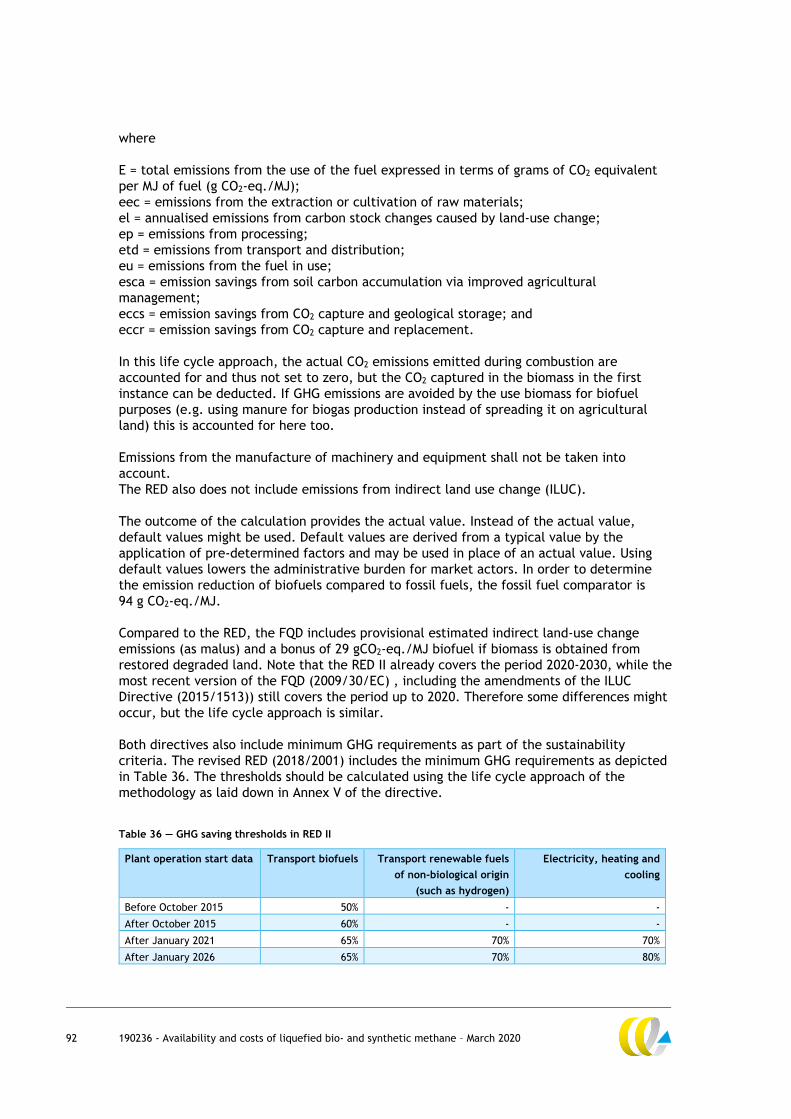
92 190236 - Availability and costs of liquefied bio- and synthetic methane – March 2020
where
E = total emissions from the use of the fuel expressed in terms of grams of CO2 equivalent
per MJ of fuel (g CO2-eq./MJ);
eec = emissions from the extraction or cultivation of raw materials;
el = annualised emissions from carbon stock changes caused by land-use change;
ep = emissions from processing;
etd = emissions from transport and distribution;
eu = emissions from the fuel in use;
esca = emission savings from soil carbon accumulation via improved agricultural
management;
eccs = emission savings from CO2 capture and geological storage; and
eccr = emission savings from CO2 capture and replacement.
In this life cycle approach, the actual CO2 emissions emitted during combustion are
accounted for and thus not set to zero, but the CO2 captured in the biomass in the first
instance can be deducted. If GHG emissions are avoided by the use biomass for biofuel
purposes (e.g. using manure for biogas production instead of spreading it on agricultural
land) this is accounted for here too.
Emissions from the manufacture of machinery and equipment shall not be taken into
account.
The RED also does not include emissions from indirect land use change (ILUC).
The outcome of the calculation provides the actual value. Instead of the actual value,
default values might be used. Default values are derived from a typical value by the
application of pre-determined factors and may be used in place of an actual value. Using
default values lowers the administrative burden for market actors. In order to determine
the emission reduction of biofuels compared to fossil fuels, the fossil fuel comparator is
94 g CO2-eq./MJ.
Compared to the RED, the FQD includes provisional estimated indirect land-use change
emissions (as malus) and a bonus of 29 gCO2-eq./MJ biofuel if biomass is obtained from
restored degraded land. Note that the RED II already covers the period 2020-2030, while the
most recent version of the FQD (2009/30/EC) , including the amendments of the ILUC
Directive (2015/1513)) still covers the period up to 2020. Therefore some differences might
occur, but the life cycle approach is similar.
Both directives also include minimum GHG requirements as part of the sustainability
criteria. The revised RED (2018/2001) includes the minimum GHG requirements as depicted
in Table 36. The thresholds should be calculated using the life cycle approach of the
methodology as laid down in Annex V of the directive.
Table 36 — GHG saving thresholds in RED II
Plant operation start data Transport biofuels Transport renewable fuels
of non-biological origin
(such as hydrogen)
Electricity, heating and
cooling
Before October 2015 50% - -
After October 2015 60% - -
After January 2021 65% 70% 70%
After January 2026 65% 70% 80%

93 190236 - Availability and costs of liquefied bio- and synthetic methane – March 2020
B Production capacity of
electrolysers
This annex analyses the production capacity of electrolysers. The electrolysers currently on
the market are either AEC or PEM. The aspects taken into account in the evaluation are:
1. Technological maturity and characteristics.
2. Efficiency (current and potential future improvement).
3. Capacity.
B.1 Technology maturity and characteristics
Table 37 shows some of the key indicators which would help us assess the current and the
future status in terms of electrolysis technology that will play a major role in the hydrogen
electrolysis hence helping us in choosing the most suitable electrolysis technology based on
few key criteria’s (Mention the criteria’s below). Both (Selma, et al., 2018) and (Imperial
College London, 2017) have been used as the source to present the below indicators. For
indicators that we could not get the latest data, we have mentioned the date aside the
indicator for reference.
Table 37 — AEC and PEM indicators based on 2015–2017 data
Indicators AEC PEM
Electrolyte Aq.potassium hydroxide Polymer membrane
Cathode Ni, Ni-Mo alloys Pt, Pt, Pd
Anode Ni, Ni-Co alloys RuO2, IrO2
Current density (A cm-2) 0.2–0.4 0.6-2.0
Voltage efficiency (%) 62-82 67-82
Operating temperature (°C) 60–80 50–80
Operating pressure < 30 < 200
Production rate (m3 H2 h-1) < 760 < 40
Gas purity (%) > 99.5 99.99
Cold start time (min) < 60 < 20
System response Seconds Milliseconds
Stack life time 60,000–90,000 20,000–60,000
Systematic lifetime (years) 20 20
Maturity Mature Commercial
Capital cost (EUR 2015/kW) 600–2,600 1,900–3,700
Operational & maintenance
cost (% to their investment
cost)
2-5% 2-5%
Electricity to hydrogen
efficiency (%)
43-69 40-69
Stack replacement cost 50% of investment cost 60% of investment cost
TRL Level 9 9
Flexibility (fluctuating
renewable electricity)
Yes Yes
Source: (Selma, et al., 2018), (E4tech, 2014) and (IRENA, 2018a).

94 190236 - Availability and costs of liquefied bio- and synthetic methane – March 2020
Efficiency
Typical efficiencies (energy output vs energy input) are currently stated to be around
65-75% for power to hydrogen using low temperature electrolysis (E&E, 2014). Currently,
electrolysers achieve their best efficiency under steady currents. PEM is better suited to
operate at partial loads and to deal with fluctuating energy supply than AEC. If the heat
released by each of these processes is recovered and used, production efficiency can
increase to 85% by 2030 (E&E, 2014) (Naimi, 2019).
Capacity
To date, about 4% of global hydrogen supply is produced via electrolysis (IRENA, 2018a).
Most of this is probably produced with AEC, which are larger scale than PEM and require
lower costs (Leeuwen, 2018), (Maria Taljegard, 2016).
Conclusion
In order to produce quantities of hydrogen that are sufficient to power a significant share of
the world fleet with synthetic methane, the capacity of electrolysers needs to increase
significantly. There are several mature technologies and most observers agree that further
technological progress is possible.

95 190236 - Availability and costs of liquefied bio- and synthetic methane – March 2020
C Levelized costs of renewable
electricity
Table 38 gives the global weighted-average Levelized Costs of Electricity (LCOE) for
renewable power plants commissioned in 2018 for the different renewable power
generation technologies for plants commissioned in 2018.
Table 38 — Global weighted-average LCOE of utility-scale renewable power generation technologies for plants
commissioned in 2018
Renewable power generation technology LCOE [USD/MWh]
Hydro 47
Onshore wind 56
Geothermal 70
Solar PV 85
Offshore wind 127
Concentrating solar power 185
Source: IRENA (2019a).
According to IRENA (2019b), the LCOE for onshore wind is already competitive compared to
all fossil fuel generation sources and is set to decline further as installed costs and
performance continue to improve.
Globally, the LCOE for solar PV is expected to fall to between 20 to 80 USD/MWh by 2030
and between 14 to 50 USD/MWh by 2050 (IRENA, 2019c).
The LCOE of offshore wind is already competitive in certain European markets and is
expected to become competitive in other markets by 2030. The LCOE of offshore wind is
expected to drop to an average between USD 50 to 90/MWh by 2030 and USD 30 to 70/MWh
by 2050 (IRENA, 2019b).

96 190236 - Availability and costs of liquefied bio- and synthetic methane – March 2020
D Production cost estimations
D.1 Ammonia
Table 39 — Production cost estimates of renewable ammonia as can be found in the literature
Source Production cost estimate Conversion to 2019 USD/MMBtu Underlying assumptions
(IEA, 2019d)
The Future of Hydrogen
Figure 31:
EU import from North
Africa: 3.8 USD/kg H2
Import to Japan from
Australia/Middle East:
4.3–5.2 USD/kg H2
EU import from North Africa:
33 USD/MMBtu
Import to Japan:
37–45 USD/MMBtu
2030 costs
Hydrogen importing costs
excluding reconversion of
ammonia to hydrogen;
transportation costs are
included.
Long term renewable
electricity price:
18-63 USD/MWh.
(Lloyd's Register; UMAS, 2019)
Fuel production cost
estimates and assumptions,
Figure 2
2030: 60 USD2019/MWh
2050: 30 USD2019/MWh
2030: 18 USD/MMBtu
2050: 9 USD/MMBtu
(Siemens Gas and Power,
2019)
Transformation: A new era
for the agri-nutrients industry
Production costs:
First projects today:
800 USD/t; 500-600 USD/t
ammonia is achievable
(mature case in 5-10 years)
Today: 45 USD/MMBtu
Mature case in 5-10 years:
28-34 USD/MMBtu
Mature case in 5-10 years:
WACC of 5%
LCOE of less than
30 USD/MWhe.
(Rivarolo, et al., 2019)
Clean Hydrogen and Ammonia
Synthesis in Paraguay from
the Itaipu 14 GW
Hydroelectric Plant
“For all the investigated sizes,
ammonia production costs are
lower than 400 EUR/ton”
[332-383 EUR/ton]
21–24 USD/MMBtu Installed power of
electrolyser scenarios:
80-600 MW
While for lower capacity
plants the fixed costs are
more significant than
variable costs (electrical
energy), for higher sizes
the situation is the
opposite, as electricity
has an higher cost
(30 EUR/MWh).
(University of Minnesota,
2019) Comparative
Technoeconomic Analysis of
Absorbent-Enhanced and
Traditional Ammonia
Production
Graph slide 14:
Levelized costs 500–
770 USD/ton ammonia
28-43 USD/MMBtu
(CE Delft, 2018b)
Waterstofroutes Nederland -
Blauw, groen en import
If produced in Morocco:
2017: 3.87 EUR2017/kg H2
2030: 2.0 EUR2017/kg H2
(NH3 production costs on top
of hydrogen production costs:
2017: 0.33 EUR2017/kg H2
2030: 0.29 EUR2017/kg H2)
If produced in Morocco:
2017: 38.4 USD/MMBtu
2030: 19.8 USD/MMBtu
(NH3 production costs on top of
hydrogen production costs:
2017: 3.3 USD/MMBtu
2030: 2.9 USD/MMBtu)
Study investigates,
amongst other things, costs
for importing green
hydrogen to the
Netherlands, with the
hydrogen being produced
in Southern Europe or
North Africa by means of

97 190236 - Availability and costs of liquefied bio- and synthetic methane – March 2020
Source Production cost estimate Conversion to 2019 USD/MMBtu Underlying assumptions
dedicated wind and solar
power. To reduce the
volume for transport,
hydrogen is assumed to be
converted into ammonia.
Electricity costs:
2017: EUR34/MWh
2030: EUR23/MWh
(Cerulogy, 2017)
What role for electromethane
and eletrocammonia
technologies in European
transport’s low carbon
future? (Figure 4)
2018 costs:
High case: 6,900 €2018/toe
Base case: 2,400 €2018/toe
Low case: 1,400 €2018/toe
2030 costs:
High case: 3,500 €2018/toe
Base case: 2,000 €2018/toe
Low case: 1,300 €2018/toe
2018 costs:
High case: 207 USD/MMBtu
Base case: 72 USD/MMBtu
Low case: 42 USD/MMBtu
2030 costs: USD/MMBtu
High case: 105 USD/MMBtu
Base case: 60 USD/MMBtu
Low case: 39 USD/MMBtu
High case: small synthesis
facility/worst case
electrolysis costs.
Low case: large synthesis
facility/best case
electrolysis costs.
(IEA, 2017c)
Renewable Energy for
Industry, From green energy
to green materials and fuels
Under the most favourable
conditions, the cost of
producing green ammonia
would be around USD 400/t
NH3, assuming an electricity
price of USD 30/MWh if
electricity is available in large
enough quantities for the load
factor of the electrolysers to
be at least 50%. The cost
under less ideal circumstances
would be USD 700/t NH3 with
electricity at USD 60/MWh and
an electrolyser load factor of
30%.
Most favourable conditions:
24 USD/MMBtu
Less ideal circumstances:
41 USD/MMBtu
(ISPT, et al., 2017)
Power to Ammonia
Business case 3 (dedicated
renewable power): NH3 costs
are between 365 and
500 EUR/ton, and with a
combination of optimistic
assumptions on CAPEX and
power price, a NH3 cost of
260-370 EUR/ton can be
achieved.
Full range: 24– 33 USD/MMBtu
Optimistic range:
17–25 USD/MMBtu
For the cost calculations of
the business cases it is
assumed that supply of NH3
will start per 1-1-2026.
(University of Oxford, 2017)
The role of ‘green’ ammonia
in decarbonising energy
2025/2030 estimate using all 5
key variables: 588 GBP/tonne
of ammonia
43 USD/MMBtu
(University of Oxford, 2015)
Analysis of Islanded Ammonia-
based Energy Storage System
This calculation returned a
LCOA value of 655 USD/ton
NH3
39 USD/MMBtu Techno-economic analysis
of an ammonia-based
energy storage system
integrated with renewable
electricity generation on
an island system (a power
network which is not
connected to the grid);

98 190236 - Availability and costs of liquefied bio- and synthetic methane – March 2020
Source Production cost estimate Conversion to 2019 USD/MMBtu Underlying assumptions
Levelized electricity cost
of the islanded system was
estimated at 251
USD/MWh.
D.2 Hydrogen
Table 40 — Production cost estimates of renewable hydrogen as can be found in the literature
Source Production cost estimate Conversion to 2019 USD/MMBtu Underlying assumptions
(IEA, 2019d)
The Future of Hydrogen,
Figure 16
2-4 USD/kg H2 17-35 USD/MMBtu 2030 hydrogen production
costs in Europe.
(IRENA, 2019d)
Hydrogen: A renewable
energy perspective
Hydrogen production costs:
average wind: 3.2 USD/kg
H2;
average PV: 2.8 USD/kg H2.
Hydrogen production costs:
average wind: 28 USD/MMBtu;
average PV: 25 USD/MMBtu.
2030 costs.
(Lloyd's Register; UMAS, 2019)
Fuel production cost
estimates and assumptions,
Figure 2
35 USD2019/MWh 10 USD/MMBtu 2030 costs; hydrogen from
renewable electricity
(liquefaction storage).
(CE Delft, 2018b)
Waterstofroutes Nederland -
Blauw, groen en import
1.7-2.9 EUR2017/kg H2 18-30 USD/MMBtu 2030 production costs,
depending on production
location (Morocco or
Netherlands).
2.2 EUR2017/kg H2 23 USD/MMBtu 2030 costs including
transportation from
Morocco to the
Netherlands, excluding
liquefaction costs.
(FVV, 2018),
Defossilisierung des
Transportsektors, Optionen
und Voraussetzungen in
Deutschland
Local production:
0.18 EUR/kWh
Centralized production:
0.08 EUR/kWh
Local production: 28 USD/MMBtu
Centralized production:
63 USD/MMBtu
2030 low cost scenario
(high efficiency, low
electricity prices from
MENA region); centralized
production: non-dedicated
renewable electricity
production.
(Frontier Economics, 2017)
PtG/PtL-Rechner:
Berechnungsmodell zur
Ermittlung der Kosten von
Power-to-Gas (Methan) und
Power-to-Liquid. Model
version 1.0
5-13 EUR Cent2017/kWh H2 18-45 USD/MMBtu 2030 production costs,
depending on production
location (Iceland, Middle
East, North Africa,
Germany).
(IRENA, 2019d)
Hydrogen: A renewable
energy perspective
Hydrogen production costs:
average wind: 2 USD/kg H2;
average PV: 1 USD/kg H2.
Hydrogen production costs:
average wind: 17 USD/MMBtu;
average PV: 9 USD/MMBtu.
2050 costs.
(Lloyd's Register; UMAS, 2019)
Fuel production cost
estimates and assumptions.
(Figure 2)
20 USD2019/MWh 6 USD/MMBtu 2050 costs; hydrogen from
renewable electricity
(liquefaction storage).
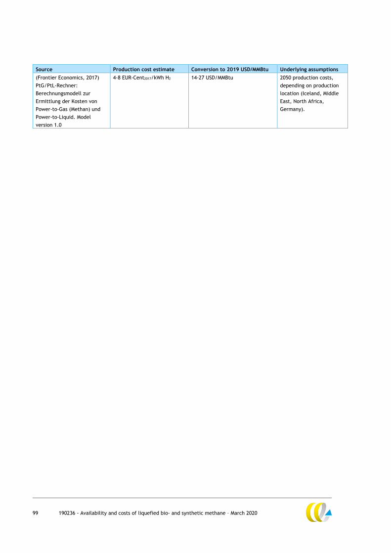
99 190236 - Availability and costs of liquefied bio- and synthetic methane – March 2020
Source Production cost estimate Conversion to 2019 USD/MMBtu Underlying assumptions
(Frontier Economics, 2017)
PtG/PtL-Rechner:
Berechnungsmodell zur
Ermittlung der Kosten von
Power-to-Gas (Methan) und
Power-to-Liquid. Model
version 1.0
4-8 EUR-Cent2017/kWh H2 14-27 USD/MMBtu 2050 production costs,
depending on production
location (Iceland, Middle
East, North Africa,
Germany).