Automatic Transition Prediction for Three-Dimensional Aircraft Configurations using the DLR TAU Code

A. KRUMBEIN1, N. KRIMMELBEIN2 and G. SCHRAUF3 1,2Deutsches Zentrum für Luft- und Raumfahrt e.V. (DLR), Institute of

Aerodynamics and Flow Technology (AS), C2A2S2E, 1Bunsenstraße 10, 37073 Göttingen, Germany, andreas.krumbein@dlr.de

2Lilienthalplatz 7, 38108 Braunschweig, Germany, normann.krimmelbein@dlr.de 3Airbus, Airbus Allee 1, 28199 Bremen, Germany, geza.schrauf@airbus.com

Summary A Reynolds-averaged Navier-Stokes solver, a laminar boundary-layer code and a fully automated local, linear stability code for the prediction of Tollmien-Schlichting and cross flow instabilities were coupled for the automatic prediction of laminar-turbulent transition on general aircraft configurations during the ongoing flow computation. The procedure is applied to different three-dimensional wing-body configurations and the sensitivity of the coupled system to a variety of coupling parameters is investigated.

1 Introduction Besides wind tunnel testing and flight tests, computational fluid dynamics (CFD) simulation based on Reynolds-averaged Navier-Stokes (RANS) solvers has become a standard design approach in industry for the design of aircraft. For the design point of aircraft a positive assessment of the numerical results was achieved for many validation and application tests and the prediction capabilities of the software tools could be positively evaluated. As a consequence, high confidence in numerical simulations could be achieved in industry and will eventually allow more simulation and less physical testing. However, and despite of the progress that has been made in the development and application of RANS-based CFD tools, there is still the need for improvement, for example, with regard to the capability of a proper capturing of all relevant physical phenomena. This can only be achieved if capable and accurate physical models are available in the codes. On the one hand, the combined use of turbulence and transition models is indispensable for flows exhibiting separation, because otherwise the close interaction between the laminar-turbulent transition and its impact on flow separation is not reproduced. On the other hand, it is not possible to fully exploit the high potential of today’s advanced turbulence models if transition is not taken into account. Thus, in modern high-fidelity CFD tools a robust transition modeling must be established together with reliable and effective turbulence models. The unstructured/hybrid RANS solver TAU, [14], [4] and [15], has been provided with a general transition prediction functionality which can be applied to general three-dimensional aircraft configurations. The developments and first technical validation steps were carried out at the Institute of Fluid Mechanics (ISM) of the University of Braunschweig, [10], [2] and [3]. The code can be used together with a laminar boundary-layer method, [1], for the calculation of highly accurate laminar boundary-layer data. Alternatively, the boundary-layer data can be directly extracted from the RANS solution. A fully automated, local linear stability code, [13], analyzes the laminar boundary layer and detects transition due

to Tollmien-Schlichting or cross flow instabilities. The stability code, which applies the eN-method, [16] and [18], and the two N factor approach, [11], [17] and [12], for the determination of the transition points, uses a frequency estimator for the detection of the relevant regions of amplified disturbances for Tollmien-Schlichting instabilities and a wave length estimator for cross flow instabilities. The stability code is now used instead of the eN-database methods which have a more limited application range and which were applied usually in an automated process chain coupling a RANS solver and a transition prediction tool, [5] and [6]. Recently, the transition prediction module of the TAU code was applied to two-dimensional airfoil configurations, the horizontal tail plane of a generic aircraft configuration and a wing-body configuration with three-element high-lift wing, [7] - [9]. In this paper, the TAU code with transition prediction is applied to three-dimensional wing-body configurations. The computations were carried out on big cluster systems with partially considerable numbers of processors. The investigations have two main purposes: Firstly, the sensitivity of the complete coupled system to a variety of the most important coupling parameters must be known in order to ensure a fast and reliable computation. Secondly, the influence of the number of grid domains (or processors, respectively) and the distribution of domains on the solution must be assessed. Both aspects can have an impact on the convergence of the transition locations and the convergence of the computation as a whole and influence the quality of the solution. For both aspects, a number of best practice statements can be derived. The results represent a first step towards the industrialization of the TAU transition prediction module.

2 Transition Prediction Coupling For production purposes, the transition prediction module applies a laminar boundary-layer method for a fast and highly accurate computation of the laminar boundary layers. The TAU code communicates the surface cp-distribution as input data to the laminar boundary-layer method COCO, [1], and COCO computes all of the boundary-layer parameters that are needed for the stability code LILO, [13]. Based on the stability analysis done by LILO eN-methods for Tollmien-Schlichting and cross flow instabilities determine transition locations that are communicated back to the TAU code. This coupling structure results in an iteration procedure for the transition locations within the iterations of the RANS equations. The structure is outlined graphically in Fig. 1. During the computation, the TAU code is stopped after a certain number of iteration cycles usually when the lift has sufficiently converged, the transition module is called and transition points are determined and fixed in the computational grid. This is done consecutively for all upper and lower sides of all specified wing sections which are defined by ‘line-in-flight’ cuts, that is, the wing is cut through parallel to the oncoming flow, according to strip theory. When all new transition locations have been communicated back, each transition location is slightly underrelaxed to damp oscillations in the convergence history of the transition points. This means that only a certain percentage of the currently determined transition point is taken into account and the new transition location is fixed somewhat downstream of that position given by the prediction method. Then, all underrelaxed transition points – they represent a transition line on the upper or lower surface of a wing element in form of a polygonal line – are mapped

onto the surface grid and the computation is continued. In so doing, the determination of the transition locations becomes an iteration process itself. With each transition location iteration step the effective underrelaxation is reduced until a converged state of all transition points has been obtained. In the last prediction step no underrelaxation is applied. In favour of the presentation of the current results the authors refer to the references [2] - [3] and [5] - [10] for further and much more detailed information on the transition coupling structure, the backgrounds of its construction and its different application modes.

3 Computational Results Two important coupling parameters which significantly influence the overall computational time are the underrelaxation factor and the interval length between two consecutive calls of the transition prediction module during the coupled computation. These two are the main parameters whose settings can lead to a significant computational overhead in a computation with predicted transition compared to a fully turbulent one, because the time of an interval and the time until the transition lines have converged are the main sources contributing to the additional computing time. In comparison, the contribution of the execution of the software parts of the transition module itself (infrastructure part in the solver, boundary-layer code and stability code) is of much lower impact. For these investigations, the flow over a generic wing-body configuration at cruise conditions – M∞ = 0.75, Re∞ = 18.4×106, α = 2.0° –, with settings for the critical N factors for quiet atmospheric conditions, NTS

crit = 12.0 and NCFcrit = 9.0, using a

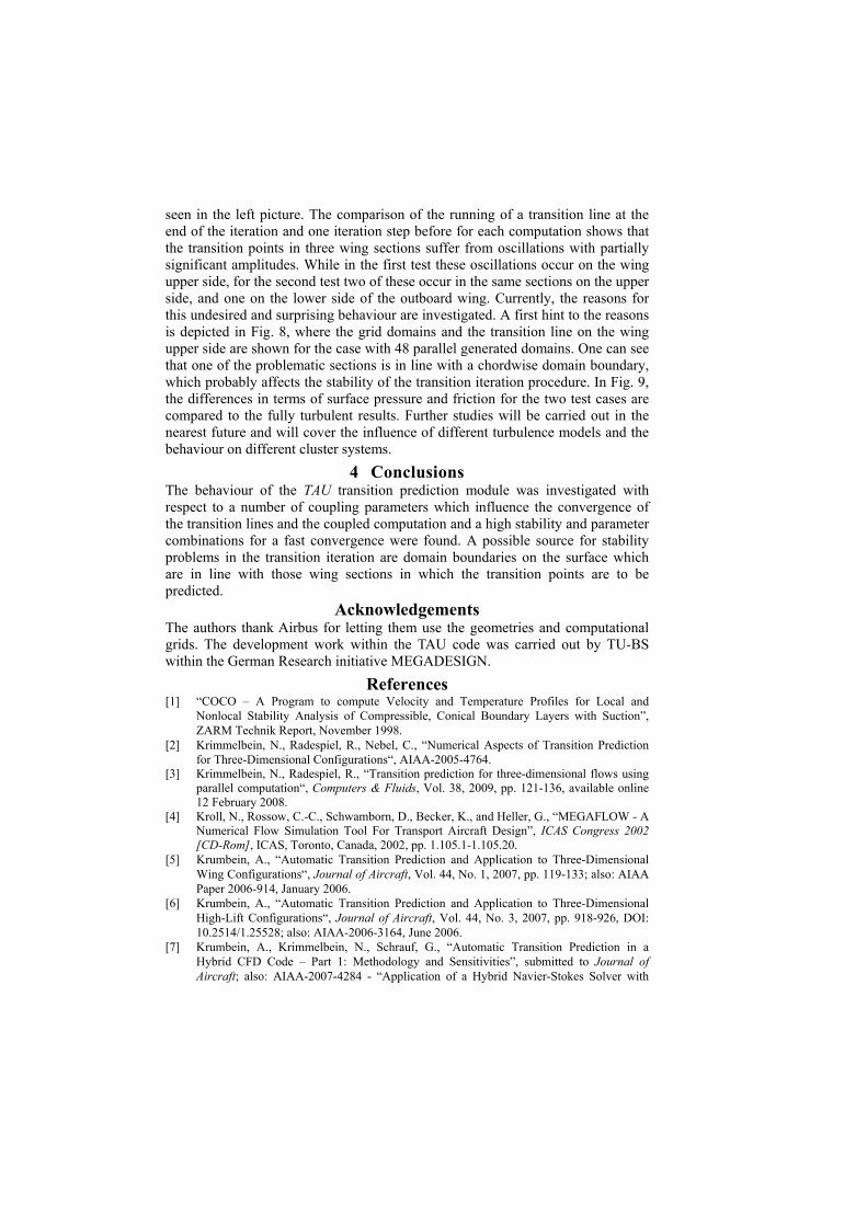
standard one-equation turbulence model was computed parallel on a hybrid grid with 9.5 million points on the C2A2S2E Linux cluster using 96 processes. As depicted in Fig. 2, all transition lines at the end of the computations with underrelaxation factors frelax = 0.5, 0.7, and 0.85 (where frelax = 0.7 means that 70% of the currently predicted transition point are taken into account) have the same converged positions, which documents the independence of the final result of the transition prediction procedure over a wide range of frelax. Fig. 3 (above) shows the impact of frelax on the global RANS convergence history in terms of the density residual and the lift and drag coefficients, CL and CD. frelax = 0.7 results in a significant convergence acceleration compared to the standard setting frelax = 0.5, while frelax = 0.85 has a slight negative influence, because it leads to a mild oscillatory behaviour with a slower convergence affecting mainly the drag. In these computations the prediction interval between two consecutive calls of the transition module was ipred = 500 cycles. In the lower picture of Fig. 3, the results for frelax = 0.7 and 0.85 are compared with those obtained for ipred = 250 and 150 cycles. As one can see, the convergence is accelerated once more leading to converged force coefficients after about 1.500 to 2.000 RANS cycles which is a factor 1.5 to 2 compared to a fully turbulent computation. The fastest convergence is obtained using the combination frelax = 0.7 and ipred = 150 cycles. In Fig. 4, the corresponding convergence histories of the transition lines show that with frelax = 0.7 and 0.85 convergence is reached after four to five calls of the transition module and that the short prediction intervals lead to the same running of the transition lines in each transition iteration step independent of the settings of ipred.

In the second but last transition point on the wing upper side towards the tip, one can see an overshoot of the solution in the first iteration steps in upstream direction and how the overshoot is slowly shifted downstream to its final position. This effect is most pronounced for frelax = 0.85 which explains the affection of the RANS convergence history of the drag. From these results it can be concluded that for this type of flow (attached, shock without separation) one can expect a smooth and fast convergence for the range 0.65 ≤ frelax ≤ 0.8. From these results it becomes clear that for a further industrialization of the transition prediction module a pointwise automatic shut-down of the transition iteration procedure, on the one hand, and sensors for a proper balancing of the settings of the underrelaxation factor and the interval length, on the other hand, are needed, whereas it is felt that the latter is of higher importance in this context. In addition, the interaction between the transition prediction procedure and the iteration of the angle of attack for a target lift computation (CL = 0.48) was tested for target lift intervals ilift = 50, 100, 200 cycles with the settings frelax = 0.7 and for ipred = 250 cycles. Fig. 5 shows that all computations converge to the same solutions in terms of the force coefficients as well as the transition lines. The fastest convergence was found for ilift = 50. The next investigation was done for the TELFONA pathfinder wing-body configuration – M∞ = 0.78, Re∞ = 20.0×106, α = 0.44°, standard one-equation turbulence model – on a hybrid grid with 14.7 million points on the C2A2S2E cluster and another, smaller Linux cluster of the institute. Here, a possible dependence on the number of grid domains (processes) and on the setting of the critical N factors was investigated. The first comparison is shown in Fig. 6. In the left picture the RANS convergence histories for 16, 32, 48, 64, and 96 grid domains are depicted for NTS

crit = 12.0, NCFcrit = 9.0, frelax = 0.5 and ipred = 250

cycles showing a smooth and long convergence of the lift and only a slight influence due to the different number and shapes of the grid domains. The same minor effect was found for NTS

crit = NCFcrit = 8.5, critical N factors which were

determined in a recently done wind tunnel campaign, for 48, 64, and 96 grid domains, whereas here the lift converges much faster, as can be seen in the left picture. In both tests the converged drag is significantly smaller than the fully turbulent one, due to the large portions of laminar flow on both sides of the wing. Why the converged lift values are smaller than the fully turbulent one in both cases is currently under investigation. Moreover, the influence of grid domains which were generated using a parallel partitioning process in contrast to the sequential partitioning which was applied for all other computations is shown in the left picture of Fig. 6. Slight differences in the shapes and spatial positions of the 48 domains in each case lead to different convergence histories here, while the computations end up with the same converged values. A look to the transition lines of both tests at the end of the transition iteration (thick dashed) and one iteration step before (thin solid), however, reveal that there is a visible influence on the location of the transition lines as well as on their convergence behaviour, Fig. 7. The comparison of the running of the different lines at the end of the iteration shows the strongest congruence for the results of 96 sequentially generated domains and 48 parallel generated domains for the first test, as can be

seen in the left picture. The comparison of the running of a transition line at the end of the iteration and one iteration step before for each computation shows that the transition points in three wing sections suffer from oscillations with partially significant amplitudes. While in the first test these oscillations occur on the wing upper side, for the second test two of these occur in the same sections on the upper side, and one on the lower side of the outboard wing. Currently, the reasons for this undesired and surprising behaviour are investigated. A first hint to the reasons is depicted in Fig. 8, where the grid domains and the transition line on the wing upper side are shown for the case with 48 parallel generated domains. One can see that one of the problematic sections is in line with a chordwise domain boundary, which probably affects the stability of the transition iteration procedure. In Fig. 9, the differences in terms of surface pressure and friction for the two test cases are compared to the fully turbulent results. Further studies will be carried out in the nearest future and will cover the influence of different turbulence models and the behaviour on different cluster systems.

4 Conclusions The behaviour of the TAU transition prediction module was investigated with respect to a number of coupling parameters which influence the convergence of the transition lines and the coupled computation and a high stability and parameter combinations for a fast convergence were found. A possible source for stability problems in the transition iteration are domain boundaries on the surface which are in line with those wing sections in which the transition points are to be predicted.

Acknowledgements The authors thank Airbus for letting them use the geometries and computational grids. The development work within the TAU code was carried out by TU-BS within the German Research initiative MEGADESIGN.

References [1] “COCO – A Program to compute Velocity and Temperature Profiles for Local and

Nonlocal Stability Analysis of Compressible, Conical Boundary Layers with Suction”, ZARM Technik Report, November 1998.

[2] Krimmelbein, N., Radespiel, R., Nebel, C., “Numerical Aspects of Transition Prediction for Three-Dimensional Configurations“, AIAA-2005-4764.

[3] Krimmelbein, N., Radespiel, R., “Transition prediction for three-dimensional flows using parallel computation“, Computers & Fluids, Vol. 38, 2009, pp. 121-136, available online 12 February 2008.

[4] Kroll, N., Rossow, C.-C., Schwamborn, D., Becker, K., and Heller, G., “MEGAFLOW - A Numerical Flow Simulation Tool For Transport Aircraft Design”, ICAS Congress 2002 [CD-Rom], ICAS, Toronto, Canada, 2002, pp. 1.105.1-1.105.20.

[5] Krumbein, A., “Automatic Transition Prediction and Application to Three-Dimensional Wing Configurations“, Journal of Aircraft, Vol. 44, No. 1, 2007, pp. 119-133; also: AIAA Paper 2006-914, January 2006.

[6] Krumbein, A., “Automatic Transition Prediction and Application to Three-Dimensional High-Lift Configurations“, Journal of Aircraft, Vol. 44, No. 3, 2007, pp. 918-926, DOI: 10.2514/1.25528; also: AIAA-2006-3164, June 2006.

[7] Krumbein, A., Krimmelbein, N., Schrauf, G., “Automatic Transition Prediction in a Hybrid CFD Code – Part 1: Methodology and Sensitivities”, submitted to Journal of Aircraft; also: AIAA-2007-4284 - “Application of a Hybrid Navier-Stokes Solver with

Automatic Transition Prediction”. [8] Krumbein, A., Krimmelbein, N., “Navier-Stokes High-Lift Airfoil Computations with

Automatic Transition Prediction using the DLR TAU Code”, Notes on Numerical Fluid Mechanics and Multidisciplinary Design · Volume 96, New Results in Numerical and Experimental Fluid Mechanics VI, Contributions to the 15th STAB/DGLR Symposium, Darmstadt, Germany 2006, Editors: Cameron Tropea, Suad Jakirlic, Hans-Joachim Heinemann, Rolf Henke, Heinz Hönlinger, pp. 210-218, Springer Verlag, Berlin-Heidelberg-New York, 2007.

[9] Krumbein, A., Krimmelbein, N., Schrauf, G., “Automatic Transition Prediction in a Hybrid CFD Code – Part 2: Practical Application”, submitted to Journal of Aircraft; also: AIAA-2008-413 – “Automatic Transition Prediction for High-Lift Configurations using a Hybrid CFD Code”.

[10] Nebel, C., Radespiel, R., and Wolf, T., “Transition Prediction for 3D Flows Using a Reynolds-Averaged Navier-Stokes Code and N-Factor Methods“, AIAA-2003-3593.

[11] Rozendaal, R. A., “Natural Laminar Flow Flight Experiments on a Swept Wing Business Jet-Boundary-Layer Stability Analysis”, NASA CP 3975, March 1986.

[12] Schrauf, G., “Large-Scale Laminar-Flow Tests Evaluated with Linear Stability Theory”, Journal of Aircraft, Vol. 41, No. 2, March/April 2004, pp. 224-230.

[13] Schrauf, G., “LILO 2.1 User’s Guide and Tutorial”, Bremen, Germany, GSSC Technical Report 6, originally issued Sep. 2004, modified for Version 2.1 July 2006.

[14] Schwamborn, D., Gerhold, T., Hannemann, V., “On the Validation of the DLR-TAU Code”, New Results in Numerical and Experimental Fluid Mechanics II, Notes on Numerical Fluid Mechanics, Vol. 72, Braunschweig, Wiesbaden, Vieweg Verlag, 1999, pp. 426-433.

[15] Schwamborn, D., Gerhold, T., Heinrich, R., “The DLR TAU-Code: Recent Applications in Research and Industry”, European Conference on Computational Fluid Dynamics, ECCOMAS CFD 2006, Egmond aan Zee, The Netherlands, 5 – 8 September 2006, ECCOMAS CFD 2006 - CD-Rom Proceedings, editors: P. Wesseling, E. Oñate, J. Périaux, 2006, ISBN: 90-9020970-0, © TU Delft, The Netherlands.

[16] Smith, A.M.O., Gamberoni, N., “Transition, Pressure Gradient and Stability Theory“, Douglas Aircraft Company, Long Beach, Calif. Rep. ES 26388, 1956.

[17] Stock, H. W., “Infinite Swept Wing RANS Computations with eN Transition Prediction – Feasibility Study”, Rept. IB 124-2003/12, Deutsches Zentrum für Luft- und Raumfahrt (DLR), Braunschweig, Germany, Aug. 2002.

[18] van Ingen, J.L., “A suggested Semi-Empirical Method for the Calculation of the Boundary Layer Transition Region“, University of Delft, Dept. of Aerospace Engineering, Delft, The Netherlands, Rep. VTH-74, 1956.

Fig. 1 Coupling structure.

Fig. 8 Grid domains and predicted transition line on the upper side of the TELFONA pathfinder wing.

Fig. 2 cf-distribution on wing-body configuration, cp-distribution and transition lines for different un- derrelaxation factors on the wing upper side.

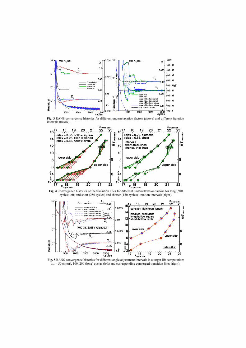
Fig. 3 RANS convergence histories for different underrelaxation factors (above) and different iteration intervals (below).

Fig. 4 Convergence histories of the transition lines for different underrelaxation factors for long (500

cycles; left) and short (250 cycles) and shorter (150 cycles) iteration intervals (right).

Fig. 5 RANS convergence histories for different angle adjustment intervals in a target lift computation;

ilift = 50 (short), 100, 200 (long) cycles (left) and corresponding converged transition lines (right).

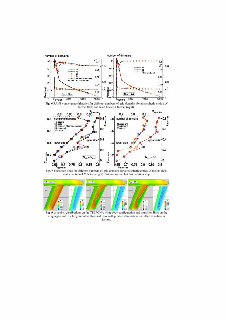
Fig. 6 RANS convergence histories for different numbers of grid domains for atmospheric critical N

factors (left) and wind tunnel N factors (right).

Fig. 7 Transition lines for different numbers of grid domains for atmospheric critical N factors (left)

and wind tunnel N factors (right): last and second but last iteration step

Fig. 9 cf- and cp-distributions on the TELFONA wing-body configuration and transition lines on the

wing upper side for fully turbulent flow and flow with predicted transition for different critical N factors.