Forecasting Swiss Exports using Bayesian Forecast ...
33
ISSN 1440-771X Department of Econometrics and Business Statistics http://business.monash.edu/econometrics-and-business- statistics/research/publications July 2019 Working Paper 14/19 Forecasting Swiss Exports using Bayesian Forecast Reconciliation Florian Eckert, Rob J Hyndman and Anastasios Panagiotelis
Transcript of Forecasting Swiss Exports using Bayesian Forecast ...

ISSN 1440-771X
Department of Econometrics and Business Statistics
http://business.monash.edu/econometrics-and-business-statistics/research/publications
July 2019
Working Paper 14/19
Forecasting Swiss Exports using Bayesian Forecast Reconciliation
Florian Eckert, Rob J Hyndman and Anastasios
Panagiotelis

Forecasting Swiss Exports using BayesianForecast Reconciliation
Florian Eckert∗†, Rob J. Hyndman‡, and Anastasios Panagiotelis‡
†KOF Swiss Economic Institute, ETH Zurich‡Department of Econometrics and Business Statistics, Monash University
July 2019
Abstract
This paper conducts an extensive forecasting study on 13,118 time series measur-ing Swiss goods exports, grouped hierarchically by export destination and productcategory. We apply existing state of the art methods in forecast reconciliation andintroduce a novel Bayesian reconciliation framework. This approach allows for explicitestimation of reconciliation biases, leading to several innovations: Prior judgment canbe used to assign weights to specific forecasts and the occurrence of negative reconciledforecasts can be ruled out. Overall we find strong evidence that in addition to produc-ing coherent forecasts, reconciliation also leads to improvements in forecast accuracy.
JEL Classification: C32, C53, E17Keywords: Hierarchical Forecasting, Bayesian Forecast Reconciliation, Swiss Ex-ports, Optimal Forecast Combination.
∗Corresponding Author: Leonhardstrasse 21, 8092 Zürich, [email protected], +41 44 632 29 80

1 Introduction
Export forecasts can support economic policy makers, monetary authorities and exportingfirms in making decisions. They may be of interest in their own right but also as inputsinto projections of other important macroeconomic quantities such as currency reserves,exchange rates and production growth. As exports of goods are usually measured andpublished on a highly disaggregate basis, many economic agents are interested in forecastsat a more granular level. For instance, a Swiss manufacturer of precision instruments isconcerned about exports of Swiss watches into individual countries in order to managetheir inventories. The large collection of 13,118 time series on Swiss goods exports issubject to known linear hierarchical constraints. Total exports from Switzerland can bedisaggregated geographically by destination into regions such as Europe, North America orAustralia. These regional aggregates can then be divided further by country. Total exportscan also be disaggregated into product categories such as precision instruments, textilesor vehicles and then further into subcategories such as road, rail, air and water vehicles.As such, the data has the structure of a so-called grouped hierarchy (see Hyndman andAthanasopoulos, 2018, and references therein). Figure 1 gives a simple example of groupedstructure with k = 3 levels, m = 9 series in total and q = 4 series at the most disaggregateor ‘bottom’ level.
Y0
YA
YA1 YA2
YB
YB1 YB2
Y0
Y1
YA1 YB1
Y2
YA2 YB2
Figure 1: Simple Example of a Grouped Hierarchy.
Since it is known that all future realizations of the data will adhere to the constraintsimplied by the aggregation structure, a desirable property of any forecasts is that they alsorespect these constraints. Such forecasts are referred to as ‘coherent’. In the case of Swissexports, incoherent forecasts are problematic because they may lead to contradictory con-clusions, non-aligned decision making and are difficult to communicate. Earlier literaturereduced the issue of producing coherent forecasts to one of predicting only a specific levelof the hierarchy. For example, the ‘bottom-up’ approach (Gross and Sohl, 1990) achievescoherence by producing only forecasts for the bottom level series and then summing theseup according to the hierarchical structure. A major shortcoming of this approach is thatdisaggregate series tend to be noisy and there is a high risk of model misspecification.Features such as seasonality may be difficult to identify in the bottom level data, despitebeing clearly present in the aggregate series. To address this shortcoming a ‘top-down’ ap-proach was proposed (see Athanasopoulos et al., 2009, and references therein), where thepredicted top level series is disaggregated according to historical or forecasted proportions
1

of lower levels. A compromise is given by the ‘middle-out’ approach, where the forecastsat an intermediate level of the hierarchy are summed up to get the higher levels and dis-aggregated to obtain lower level predictions. A weakness of these single level methods isinformation loss because the time series characteristics at other levels are not taken intoaccount. A further shortcoming of the middle-out and top-down methods is that they arenot easily applied to grouped hierarchical structures.
In response to these shortcomings, there has been a tendency over the past decadetowards producing forecasts for all series in the hierarchy rather than only at a singlelevel. These are referred to as ‘base’ forecasts and they generally do not adhere to ag-gregation constraints. ‘Forecast reconciliation’, introduced by Hyndman et al. (2011),performs an ex-post adjustment to base forecasts in order to produce a new set of co-herent forecasts. This adjustment effectively combines predictions from all levels and indoing so ‘hedges’ against misspecification error across all levels. There is now substantialtheoretical and empirical evidence that forecast reconciliation can significantly improveforecast accuracy (see Wickramasuriya et al., 2018, and references therein). The firstmain contribution of our own paper is therefore to apply existing reconciliation methodsto the problem of forecasting Swiss export data.
Despite their success, forecast reconciliation methods suffer a number of shortcomings,some arising in general and others due to the idiosyncrasies of our dataset. First, forecastreconciliation can induce negative forecasts even when the base forecasts are non-negative.This is clearly problematic when forecasting quantities that must be non-negative byconstruction. Second, an important theoretical assumption to ensure optimality of forecastreconciliation is that forecasts are unbiased prior to reconciliation. Often this assumptionfails to hold in practice. Third, existing reconciliation methods combine forecasts in away that is backward-looking, combining models using weights that depend on the inverseof past variation of forecast errors. There are several instances where this approach maybreak down for our dataset. One is the case of exports to small trading partners whichare zero for most (and in some cases all) of the observations in the training sample. Thesecan be predicted almost perfectly by a naive forecast of zero, leading to no variationin the forecast errors and numerically unstable reconciliation. Another case where thebackward-looking nature is inappropriate occurs when forecasters have information that aforecasting model may break down even if it has performed well in the past. An exampleof this in our dataset is a structural break induced by the reclassification of electricity as agood rather than a service. Finally, the backward-looking nature of existing reconciliationmethods also makes it difficult to exploit information from the entire predictive density ofa forecast target.
The second major contribution of our paper is to extend existing forecast reconciliationin a way that addresses these shortcomings. The main innovation is to convert the generalreconciliation equation into a panel regression. Rather than using a single vector of point
2

forecasts, we draw samples from the predictive densities of the base forecast models. Thispanel regression is estimated using Bayesian Markov Chain Monte Carlo algorithms. Ourapproach has a number of benefits relative to the existing methodology. First, reconcil-iation biases in the base forecasts are made explicit by introducing fixed effects into thepanel regression structure. This overcomes a major weakness of existing approaches whichrequire base forecasts to be unbiased to ensure that reconciliation is optimal. Second,we propose a mechanism for down-weighting the influence of particular series irrespectiveof past forecasting performance. This is valuable if forecasters have strong judgmentalreasons for believing that a particular model will work well in the future while other baseforecasts will be less reliable. Third, under our approach, the weights used in reconciliationcan depend on the variances of the predictive density rather than in-sample forecast errors.Existing approaches essentially determine weights based on estimates of the unconditionalvariance. Our innovation is therefore particularly promising for forecasting models thatallow for conditional heteroskedasticity. Fourth, the Bayesian estimation procedure conve-niently allows the incorporation of prior information to solve issues such as the occurrenceof negative reconciled forecasts and singular forecast error covariance matrices.
The remainder of the paper is structured as follows. Section 2 introduces in detailthe data on exports of Swiss goods, using modern techniques for exploring and visualizinghigh-dimensional time series. Section 3 introduces both existing forecast reconciliation aswell as our novel Bayesian approach. Section 4 conducts an extensive forecast evaluationthat compares our proposed method with existing reconciliation techniques. Section 5concludes.
2 Data
We use a comprehensive dataset containing exports of Swiss goods. All time series covera period from 1988 to 2018 in monthly frequency and are denominated in Swiss francs.They are not adjusted for seasonalities or calendar effects. The data can be grouped byexport destination and product category. The geographic hierarchy consists of 8 regions,aggregated from 245 countries and dependent territories. The categorical hierarchy followsa national nomenclature covering 12 main economic groups and 48 subgroups1. This leadsto a grouped hierarchy with m = 13, 118 series containing at least one nonzero entry ofwhich q = 9, 483 series are at the bottom level. Figure 2 shows the historical developmentof the regional and categorical hierarchies.1Precious metals, precious and semi-precious stones, works of art and antiques are generally omitted inbusiness cycle research due to volatility and structural breaks.
3

by R
egio
nby
Cat
egor
y
1990 1995 2000 2005 2010 2015
0
5
10
15
20
0
5
10
15
20
Mon
thly
Exp
orts
(in
bill
ion
CH
F)
Regions
Europe (53.4%)
North America (17.8%)
East Asia (16.6%)
Africa and Middle East (5.3%)
Latin America (3.0%)
Central Asia (1.5%)
South Asia (1.0%)
Australia and Oceania (1.3%)
Categories
Chemicals and Pharmaceuticals (44.7%)
Precision Instruments (21.3%)
Machines and Electronics (14.4%)
Metals (6.2%)
Agricultural Products (4.3%)
Vehicles (2.2%)
Textiles (2.1%)
Leather, Rubber, Plastics (2.0%)
Energy Source (1.2%)
Graphical Products (0.7%)
Various Goods (0.6%)
Stones and Earth (0.4%)
Figure 2: Contribution to Swiss Exports of Goods. Nominal values, not adjusted forseasonalities or calendar effects. Average export shares of the year 2018 in parentheses.
As a result of its status as a small open economy in a rapidly globalizing world, Swissexports have increased significantly since the late 1980s. Accounting for more than half oftotal exports, Europe is a key market for Swiss goods. Increasingly larger shares of exportsalso go to North America and East Asia with around 17% each in 2018. Exports to Africaand the Middle East, Latin America, Central and South Asia and Australia account onlyfor about 10% combined.
The hierarchical grouping by categories is more evenly distributed, but has been subjectto greater shifts in its composition. The most important categories are ‘Chemicals andPharmaceuticals’, ‘Precision Instruments’ and ‘Machines and Electronics’. Figure 3 showsthe changes in composition between 1988 and 2018.
4

Germany
France
Italy
Austria
Netherlands Spain
Japan
United States
Africa andMiddle East
East Asia
Europe North America
Textiles
Plastics
Metal goods
Industrial machinery Watches
Chemicals andPharmaceuticals
Machines and Electronics
Metals
Precision Instruments
Textiles
Germany
France Italy
Spain Austria Japan
United States
East AsiaEurope
North America
Plastics
Metal goods
Industrial machinery
Watches
Chemicals and PharmaceuticalsMachines and
Electronics
Metals
Precision Instruments Textiles
in 1988 in 2018by
Reg
ion
by C
ateg
ory
0 20 40 60Regional or Categorical Share of Exports (in %)
Figure 3: Regional and Categorical Composition of Swiss Goods Exports.
The two hierarchical groupings are quite different. The geographic hierarchy with 8groups and 245 subgroups is wide, but with a majority of the export volume going toEuropean countries, it is nevertheless highly concentrated. This has changed slightly inthe past 30 years as the relative share of exports to the rest of the world has increased. Thecategorical hierarchy on the other hand is rather narrow with 12 groups and 48 subgroups.Compared to the regional hierarchy, the export volume is however more evenly distributed,even though an increasing concentration, particularly in chemicals and pharmaceuticals,can be noted.
Due to the aggregation involved, top level series are usually less noisy and exhibit morepredictable characteristics such as seasonality or trend. Following Kang et al. (2017), it ispossible to construct a measure of predictability for each time series by estimating princi-pal components from a number of time series features that are commonly associated withbetter predictability. This includes measures such as the strength of seasonality, trend,spectral entropy and serial correlation. On the vertical axis, Figure 4 shows the first prin-cipal component, which accounts for a large share of the variation in these predictabilityfeatures.
5

●
●
●
●
●
●
●
●
●
●
●
●
●
●
●
●
●
●
●
●
●
●
●
●
●
●
●
●●
●
●
●
●
●
●
●
●
●
●
●
●
●
●
●
●
●
●
●
●●
●
●
●●
●
●
●
●
●
●
●
●
●
●
●
●
●
●
●
●
●
●
●
●
●
●
●
●●
●
●
●
●
●
●● ●
●
●
●
●
●
●
●
●
●
●
●
●
●
●
●
●
●
●
●
●
●
●
●
●
●
●
●
●
●●
●
●
●
●
●
●
●
●
●
●
●
●
●
●●
●
●
●●
●
●
●
●
●
●
●
●
●
●●
●
●
●
●
●
●
●
●
●
●
●
●
●
●
●
●
●
●
●
●
●
●
●
●●
●
●
●
●
●
●
●
●
●
●
●
●
●
●
●●
●
●
●
●
●
●
●
●
●
●
●
●
●
●
●
●
●
●
●
●
●
●
●
●
●●
●
●
●
●
●
●
●
●
●●
●
●
●
●
●
●
●
●
●
●
●
●
●
●●
●
●
●
●
●
●
●
●
−2
0
2
4
6
1e+2 1e+3 1e+4 1e+5 1e+6 1e+7 1e+8 1e+9 1e+10
Export Volume (in CHF, log scale)
Pre
dict
abili
ty
Level●●
●
World
Region
Country
Region
●
●
●
●
●
●
●
●
●
Europe
North America
East Asia
Africa and Middle East
Latin America
Central Asia
South Asia
Australia and Oceania
World
Figure 4: Predictability of Different Levels in a Hierarchy. Predictability is defined as thefirst principal component of a large number of time series characteristics.
It is evident that there exists a strong correlation between predictability and exportvolume. This implies that larger series and consequently those at the top of a hierarchyare easier to forecast.
3 Forecast Reconciliation
3.1 Existing Forecast Reconciliation Methods
In order to encode the aggregation constraints in a hierarchy, we define Yt to be anm-vectorthat stacks observations at time t from all series, Bt to be a subvector of Yt containingonly the q bottom level series at time t and S to be an m× q aggregation matrix. In thesimple grouped hierarchy shown in Figure 1, these are given by
Yt(m×1)
=
Y0
YA
YB
Y1
Y2
YA1
YA2
YB1
YB2
S(m×q)
=
[columns− width = 5mm]1 1 1 11 1 0 00 0 1 11 0 1 00 1 0 11 0 0 00 1 0 00 0 1 00 0 0 1
Bt(q×1)
=
YA1
YA2
YB1
YB2
6

Here and in general, the matrix S is defined so that Yt = SBt holds for all realized data.Hyndman et al. (2011) considered a framework whereby forecasts are produced for all mseries at every level, referring to these as ‘base forecasts’. To reconcile these base forecasts,the following regression structure was assumed.
Yt(h) = Sβh + et(h), (1)
where Yt(h) is anm-vector containing the h-periods-ahead base forecasts at time t for eachlevel in the hierarchy, βh represents the true expected value of the bottom level series, andthe error term et(h) has mean zero and covariance matrix Σh. Reconciled forecasts aregiven by Sbh, where bh is an estimate of βh that combines information about forecasts atall levels. It can be estimated using the following regression equation,
bh =(S′W−1
h S)−1
S′W−1h Yt(h). (2)
This choice minimizes the generalized Euclidean distance between Yt(h) and the reconciledforecasts Sbh with respect to Wh. Reconciliation is also guaranteed to reduce the distanceto the eventual realization targeted by a forecast. There are several potential choices forWh. Letting Wh = I corresponds to an ordinary least squares estimate. Alternatively, ahigh degree of heteroskedasticity in the error terms motivates a diagonal Wh or weightedleast squares approach (Hyndman et al., 2016). Under so-called ‘variance scaling’, weightsare the variances of in-sample h-step ahead forecast variances, and forecasts with lessaccurate historical performance are down-played in reconciliation. Another alternative isthe ‘nseries’ approach due to Athanasopoulos et al. (2017), whereby weights are based onthe number of series aggregated at each node. More recently, the ‘MinT’ approach wasdeveloped by Wickramasuriya et al. (2018) to allow for a Wh that is not diagonal andexploits the covariances between the h-step-ahead reconciled forecast errors. The nomen-clature MinT refers to the fact that this approach minimizes the trace of the covariancematrix of reconciliation errors.
3.2 Bayesian Forecast Reconciliation
In this part, we propose a new methodology for forecast reconciliation. The main insightis that additional information about the uncertainty surrounding base forecasts can beincorporated into the reconciliation procedure. In the spirit of Kapetanios et al. (2015) orAmisano and Geweke (2017), the predictive distributions of the m base forecast modelsare approximated with a sample of n draws. Possible sources for obtaining these draws areposterior predictive distributions from Bayesian forecasting models, bootstrap aggregating(Bergmeir et al., 2016), model pooling, or sampling from a fitted model. This results in nvectors yi, each of length m, that contain a draw i from each predictive distribution.2
2Since every forecast horizon is reconciled independently, the time subscripts are dropped from now on tosimplify notation.
7

This allows the regression model from equation (1) to be recast as a panel regression.The error term consists of two components, a prediction error ei and a reconciliationbias α. The latter can be interpreted as a fixed effect that is unique to each forecastedvariable. In other words, α is the difference between the unreconciled forecast mean y andthe reconciled forecast mean y. The interpretation of β depends on the definition of S, butin general it estimates the mean of the bottom level reconciled forecasts. The followingequation can then be used to model the forecast reconciliation:
yi = α + S × β + ei ,
(m× 1) (m× 1) (m× q) (q × 1) (m× 1)(3)
where e follows a normal distribution with mean zero and covariance matrix Σ. The rec-onciliation problem in (3) can be expressed as a system of seemingly unrelated regressions(SUR) to account for cross-equation correlations. Since the explanatory variables are thesame for each equation, it is a special case of the SUR model in Zellner (1962). However,the parameters are impossible to estimate directly because of perfect multicollinearity inthe regressors Im and S. This is quite intuitive since there is more than one unique way toreconcile incoherent forecasts. Following Farebrother (1978), the regression is partitionedin order to separate the parameters that cause multicollinearity and they are estimatedin separate Gibbs sampling steps. The distribution of the reconciled forecasts can be ob-tained by sampling from the posterior predictive distribution conditional on α being equalto zero:
p(y | α = 0, y, S) =∫∫
p(y | α = 0, β,Σ, y, S) p(α = 0, β,Σ | y, S) dβ dΣ.
The joint posterior distribution of α, β and Σ is obtained by combining a prior belief onthe parameters with the likelihood according to Bayes’ theorem:
p(α, β,Σ | y, S) ∝ p(y, S | α, β,Σ)× p(α, β,Σ). (4)
The likelihood function of the data is given by
p(y, S | α, β,Σ) ∝ 1|Σ| exp
[−1
2∑
i
(yi − α− Sβ)′Σ−1(yi − α− Sβ)].
8

The joint posterior distribution is accordingly given by
p(α, β,Σ | y, S) ∝ 1|Σ| exp
[−1
2∑
i
(yi − α− Sβ)′Σ−1(yi − α− Sβ)]
× exp[−1
2(α− a0)′A−10 (α− a0)
]× exp
[−1
2(β − b0)′B−10 (β − b0)
]× 1|Σ|(v0 −m− 1) exp
[−1
2tr(R−10 Σ−1)
].
The Bayesian approach has the advantage that uncertainty surrounding the parameters α,β and Σ is taken into account. Following Percy (1992), we get the marginal distributionsby approximating the joint posterior distribution via Gibbs sampling from the conditionaldistributions. Convergence is achieved quickly, irrespective of the starting values. It can beverified by testing for stability in the recursive means of the Markov chains. A sufficientlylarge sample of draws from the posterior predictive distribution of y is saved and evaluatedto get summary statistics such as the mean and variance of the reconciled forecasts.
Step 1: Draw β conditional on α,Σ, y, SThe parameter β is the mean of the bottom level forecasts, given an appropriate aggrega-tion matrix S. The conditional posterior distribution is then given by
β | α,Σ, y ∼ N(b1, B1), (5)
where B1 =(∑
i S′Σ−1S +B−1
0
)−1and b1 = B1
(∑i S′Σ−1(yi − α) +B−1
0 b0). Unless
there is reason to believe otherwise, the priors b0 and B0 should be chosen to be asuninformative as possible. In some cases, this regression approach leads to negative valuesin the reconciled bottom level forecasts. This might be a concern since many applicationssuch as sales or exports do not allow for negative observations. Using a truncated normalprior, this issue can be resolved in an uncomplicated fashion by simply discarding drawsof β that contain negative entries during the sampling process.
Step 2: Draw Σ conditional on α, β, y, S
Σ is the covariance matrix of the prediction errors. While Σ is not singular by definitionbecause the forecasts in yi are not reconciled, it might be near-singular if the base fore-casting models are estimated jointly or if the draws are reordered following Jeon et al.(2018). In the latter case Σ can be drawn from an inverse Wishart distribution.
Σ | α, β, y ∼W−1(v1, R1), (6)
where v1 = v0 + n and R1 =(R−1
0 +∑
i(yi − α− Sβ)′(yi − α− Sβ))−1
. It is useful toset an almost uninformative prior with v0 and R0 close to zero, which introduces a smallamount of noise into the reconciled forecasts. This has negligible impact on the posterior
9

distribution, but ensures that Σ is nonsingular in the case where a base forecast has novariation. A possible simplification is to draw the variances equation-by-equation from aninverse gamma distribution.
Step 3: Draw α conditional on β,Σ, y, SBecause the reconciliation regression is an ill-posed problem, it is necessary to imposeadditional restrictions on the reconciliation biases α in order to achieve identification.The conditional distribution of α can be expressed equivalently by concentrating out β inthe following reconciliation identity.
α = 1n
∑i
yi − Sβ. (7)
In order to eliminate β from equation (7), both sides are multiplied by a projection matrixP . The reconciliation biases depend greatly on the definition of this projection matrixand alternative choices for P will be discussed in Section 3.3. Using P = S(S′S)−1S′
implies an orthogonal projection onto the coherent subspace. The resulting terms arethen subtracted from both sides of equation (7):
(Im − P )α = (Im − P ) 1n
∑i
yi. (8)
It is useful to define the idempotent residual maker M = Im − P . Since M is not in-vertible due to the presence of multicollinearity, equation (8) cannot be solved for α.Our identifying assumption is that α lies in the span of M in which case Mα = α. ForP = S(S′S)−1S′, this implies that the direction of the reconciliation bias is orthogonal tothe coherent subspace. This solves the identification problem and leaves the reconciliationbiases as a function of the data and the residual maker M . This result is again intuitivesince the reconciliation biases are the residuals from a regression of the base forecasts onthe aggregation matrix:
α = M
(1n
∑i
yi
). (9)
Having identified the system in that way, the prior variance A0 is allowed to be uninfor-mative and the prior mean a0 is a zero vector. A numerically stable conditional posteriorfor α is therefore given by
α | β,Σ, y ∼ N(a1, A1), (10)
where A1 = M(
Σn
)M ′ and a1 = M
(1n
∑i yi
).
10

3.3 Bias Weighting
The definition of the projection matrix P is crucial for the estimated parameters. Figure 5demonstrates the impact of different projections on the estimated reconciliation biases. Itfeatures identical unreconciled forecasts of a simple hierarchy with m = 3 series, whereYA + YB = Y0. For each series a sample is drawn from the predictive forecasts density,assumed to be N(4, 2) for YA (shown in blue), N(6, 1) for YB (shown in purple), andN(16, 3) for Y0 (shown in yellow). The horizontal axis shows draws from the unreconciledbase forecasts, which are clearly incoherent. The vertical axis on the other hand showsthe means of the reconciled forecasts. The diagonal line shows values where the means ofbase and reconciled forecasts are equal. For boxes above this diagonal line, reconciliationadjusts forecasts upwards, for boxes below the diagonal line reconciliation adjusts forecastsdownwards.
(3) GLS & Shrinkage towards Y0 (4) GLS & Shrinkage towards YA
(1) OLS (2) GLS
4 8 12 16 4 8 12 16
4
8
12
16
4
8
12
16
Unreconciled Forecast Draws
Rec
onci
led
For
ecas
t Mea
n (S
β)
Unreconciled Base Forecasts YA ~ N(4, 2) YB ~ N(6, 1) Y0 ~ N(16, 3)
Figure 5: Weighting Schemes. The grey line indicates where the unreconciled base forecastson the x-axis are equal to reconciled forecast means on the y-axis.
Each panel corresponds to a different choice of P . Using P = S(S′S)−1S′ correspondsto the orthogonal projection in an ordinary least squares regression. Subfigure (1) showsthat the forecast biases for each margin are treated equally, consequently the means of YA
and YB are adjusted upwards while the mean of Y0 is adjusted downwards. Using P =S(S′Σ−1S)−1S′Σ−1 implies that the reconciliation biases are weighted with the inverseof their corresponding forecast variances. This leads to a smaller adjustment in YB (thereconciled and base means are close) relative the others since it is more accurate.
11

Even though it is intuitive to weight the reconciliation biases using the predictiveaccuracy of the corresponding base forecasts, this can be generalized to different weight-ing schemes. There may exist prior information on the reliability of certain models or therequirement to fix some forecasts at specific values. This could be due to better data avail-ability, higher suitability of a particular model or subjective judgment of the forecaster.Weighting can be achieved using a projection matrix P = S(S′(ΛΣΛ′)−1S)−1S′(ΛΣΛ′)−1
that includes a diagonal matrix of weights Λ. It may be of interest to selectively shrinksome reconciliation biases in α towards zero by decreasing the corresponding entry in Λ.At the same time, it is necessary to increase the remaining elements such that they are ableto capture the higher reconciliation biases at their level of the hierarchy. This is achievedby keeping the total dispersion of the multivariate normal distribution ΛΣΛ′ constant. Acommon measure is the generalized variance described in Mustonen (1997) and definedas the determinant of a covariance matrix. The weighting matrix Λ is therefore alwaysconstructed such that the product of the diagonal elements remains constant at 1. Thisin turn ensures that the total dispersion of ΛΣΛ′ remains equal to the total dispersion ofthe unweighted Σ for all Λ. Subfigures (3) and (4) shrink the reconciled forecasts of Y0
and YA towards their base forecasts.
It is important to note that the likelihood is invariant to these choices. Besides theshrinkage of specific reconciliation biases towards zero, there are several other weightingmethods conceivable. Possible approaches include the weighting of each series by its levelin the hierarchy or by to the number of series at each node in the hierarchy. This allowsfor the emulation of the ‘nseries’, ‘bottom-up’, ‘middle-out’ and ‘top-down’ results. Aconvenient feature of this is that the ‘middle-out’ and ‘top-down’ shrinkage work also forgrouped time series, which is not the case in the standard approach.
4 Reconciliation of Export Forecasts
4.1 Setup
The large hierarchy of Swiss goods exports is used to test the Bayesian reconciliationframework and various competing methods. Each month from 1995 to 2015, forecastsfor all series in the hierarchy are calculated for the next 36 months. For each of the13,118 series, forecasts are calculated from three models: an autoregressive integratedmoving average model (ARIMA), an exponential smoothing state space model (ETS) anda seasonal random walk model (RW). As described in Hyndman and Khandakar (2008),the model for each series is parametrized automatically based on the Akaike InformationCriterion. In order to get samples from the predictive densities, n = 1000 sample pathsare simulated from each fitted model using Gaussian errors. With the exception of thevolatile period during the Great Recession, the ARIMA and ETS approaches outperformthe Random Walk on average for series at every level and forecasting horizon. All results
12

in the following subsection will therefore rely on ARIMA forecasts.3
These incoherent forecasts are then reconciled using several basic single level and opti-mal combination methods. The single level techniques include bottom-up, top-down andmiddle-out methods. The latter two can only be used for non-grouped time series andare therefore tested on the regional and categorical hierarchies separately. The optimalcombination methods used are ordinary and weighted least squares, nseries, MinT andBayesian reconciliation (BSR). Draws from the predictive distributions are obtained bysampling from the fitted models assuming normality of the errors. If aggregation of theprediction errors is necessary, they are weighted with their respective export share.
The resulting coherent forecasts are evaluated using several accuracy measures such asthe root mean squared error (RMSE), mean absolute percentage error (MAPE) and meanabsolute scaled error (MASE). The method of Diebold and Mariano (1995) is used to testwhether reconciled forecasts are significantly more accurate than unreconciled forecasts.The Diebold-Mariano test checks for significance in the difference between two squaredforecast errors at various forecasting horizons, accounting for serial correlation in thesquared error loss. In addition, another significance test is used to compare the meansquared errors directly. Since the prediction errors are assumed to be normally distributed,the ratio between mean squared errors of an unreconciled forecast and a specific reconciledforecast has an F -distribution with degrees of freedom corresponding to the number oferrors. This allows us to test for equality of the unreconciled and reconciled mean squaredprediction errors.
4.2 Comparative Results
This section provides empirical evidence for the benefits of optimal hierarchical combina-tion. It compares the performance of different reconciliation methods and explores whichdata characteristics profit in particular from hierarchical combination.
Benefits of Hierarchical Combination. Figure 6 shows the accuracy of forecasts,defined as the mean squared error of the base forecasts relative to the mean squared errorsof the coherent forecasts from each method. Higher bars indicate therefore better forecastperformance. The 95% confidence interval shows the acceptance region of an F -test forequality of the mean squared errors. It is worth noting that reconciliation methods andbottom-up forecasts are the only techniques that allow for coherence across all levels ofa grouped hierarchy. Top-down and middle-out reconciliations are not applicable in thecase of grouped time series.
It is evident that single level methods do not consistently improve forecasting accuracy.The bottom-up and middle out methods fare reasonably well for the top level series,but fail to outperform the unreconciled forecasts at lower levels and are sometimes even3A comparison of forecasting methods, horizons and accuracy measures can be found in Appendix A.1.
13

significantly worse. Optimal combination on the other hand tends to outperform the baseforecasts especially for top and intermediate level series. Especially the methods usingvariance scaling, such as MinT, WLS and BSR, work well at all levels.
Total Category Subcategory
Wor
ldR
egio
nC
ount
ry
SingleLevel
OptimalCombination
SingleLevel
OptimalCombination
SingleLevel
OptimalCombination
−30−1501530
−30−1501530
−30−1501530
Reconciliation Methods
Relative M
SE
Bottom−Up
Middle−Out (Categories)
Middle−Out (Regions)
Top−Down (Categories)
Top−Down (Regions)
MinT
WLS
OLS
nseries
BSR
Figure 6: Relative Accuracy of Reconciliation Methods. Higher bars indicate better fore-casts relative to the unreconciled case. The zero line shows the accuracy of unreconciled predictions,with a 95% confidence interval for the ratio of mean squared errors to be one. Average of all forecasthorizons.
Comparison of Combination Methods. It is also instructive to look at the develop-ment of the relative forecasting accuracy over time in Figure 7. Even though the variancescaling methods are more accurate on average, they do not consistently outperform theunreconciled forecasts. It also appears that MinT, WLS and BSR perform fairly similarover time. For the top level series, the benefits of reconciliation accrue mostly duringtimes of global economic distress and corresponding appreciations of the Swiss franc. Thisis due to the fact that the simpler models at lower levels provide stability at times whenthe top level model is biased. The biggest gains can be observed during the early 2000srecession following the burst of the dot-com bubble, the global financial crisis and thefollowing sovereign debt crisis in Europe, and the sudden appreciation of the Swiss francafter the Swiss National Bank stopped supporting the currency peg to the Euro in early2015. Interesting is the forecasting accuracy after January 2002, when electrical energywas reclassified as a good instead of a service. The structural break in the time seriesleads to misspecified models, but the rigid structure imposed by the hierarchy increasesforecast accuracy substantially relative to the unreconciled case.
14

Total Category SubcategoryW
orld
Reg
ion
Cou
ntry
2000 2005 2010 2015 2000 2005 2010 2015 2000 2005 2010 2015
0
200
400
600
0
200
400
600
0
200
400
600
Time
Relative M
SE
MinT WLS BSR
Figure 7: Relative Accuracy of Reconciliation Methods over Time. Higher lines indicatebetter forecasts. Zero line shows the accuracy of unreconciled predictions, with a 90% confidenceinterval for the ratio of mean squared errors to be one. Base forecasts are generated using ARIMAmodels. Average of all forecast horizons.
Significance of Results. In order to check whether the accuracy improvements aresignificant, one-sided Diebold-Mariano tests are used for the top-level series. Figure 8shows the p-values when testing for equality of reconciled and unreconciled forecasts. Thealternative hypothesis is that the accuracy of reconciliation methods is greater. With theexception of the middle-out approach, single level methods are not significantly more accu-rate than the unreconciled forecasts at all horizons. Optimal combinations are associatedwith lower P-values, in particular OLS. This perhaps reflects the stability of OLS recon-ciliation which does not require the estimation of a large weighting matrix and thereforeleads to forecast errors with a smaller variance.
15

●
●
●
●
●
● ●
●
● ●
● ●
●
●
● ●●
●●
●● ●
●●
● ●● ●
●
● ● ●
●● ●
●
●
●
●●
●
●
●
●
●
●
●● ● ●
● ●●
●
●
●
●
●●
●● ● ● ● ●
● ● ●
● ●●
●
●
●
●●
●●
●● ●
●●
●
●●
●●
●●
●● ●
●● ●
● ● ● ●●
● ● ● ●● ●
●
●
●
●
●
●
●
●
●
●
●●
●
●
●
●
●
●
●
●
●
●
● ●●
●
●
●
●
●
●
●
●
● ●
●
●
●
●
●
●
●
●●
●●
●
●●
●
●
●
●
●
●
●
●
●
●
●●
●
●
●
●
● ●
●
●
●
●
●
●
●
●
●
●
●
● ●
●
●●
● ●●
●
● ●●
●●
●●
●●
● ● ● ● ● ●● ● ●
● ● ●●
●●
● ● ● ● ● ● ● ● ● ●
●● ● ● ● ● ● ● ● ● ● ●
● ● ● ● ● ● ● ● ● ● ●●
●
●
●●
● ● ● ● ●● ● ●
● ●● ●
● ● ● ● ●● ●
● ● ● ● ● ●●
● ●● ● ●
●
●
●
●●
●
● ●● ●
● ● ●●
●● ●
● ● ● ● ●● ●
● ● ● ● ● ●●
● ●● ● ●
●
●
●
●
●
●● ●
●●
●● ●
● ●
● ●● ●
● ●●
●●
● ● ● ● ● ●●
● ●● ● ●
●
Single Level Optimal Combination
10 20 30 10 20 300.0
0.2
0.4
0.6
0.8
1.0
Forecast Horizon (in Months)
P−
Val
ues
of D
iebo
ld−
Mar
iano
Tes
t
●
●
●
●
●
●
●
●
●
●
Bottom−Up
Middle−Out (Categories)
Middle−Out (Regions)
Top−Down (Categories)
Top−Down (Regions)
MinT
WLS
OLS
nseries
BSR
Figure 8: Significance of Forecast Accuracy Improvements. Test for top-level total exportsseries, where points indicate p-values of Diebold-Mariano test for greater accuracy of reconciledversus unreconciled forecasts. Lines indicate locally estimated scatterplot smoothed (LOESS) p-values.
Implications for Data Characteristics. Another way to dissect the results is to iden-tify which time series see the greatest gains in forecast accuracy from using reconciliation.Figure 9 provides an overview of the relative forecast accuracy by geographic classification,using the Bayesian reconciliation framework. It is again obvious that reconciled forecastsare on average more accurate than in the unreconciled case, but not in every instance. Itappears that series with a larger export volume benefit most from reconciliation. Forecastsof exports to countries in Europe, North America and East Asia are almost entirely betteroff than in the unreconciled case, whereas forecasts of exports to countries with a lowershare, such as the islands in Oceania, tend to be worse off. In addition, time series athigher levels in a hierarchy do not necessarily profit more from reconciliation than theircorresponding subcategories.
16

●●
●
●
●
●
●
●
●
●
●
●
●
●
●
●
●
●●
●
●
●
●●
●
●
●
●
●
●●
●
●
●●
●
● ●
●●
●
●
●
●
●
●
●
●
●●
●
●
●
●
●
●
●
●
●
●
●
●
●
●
●
●
●
●
●
●
●
●
●
●
●
●
●
●
● ●
●
●
●
●
●
●
●
●
●
●
●
●
● ●
●
●
●
●
●●
●
●●
●●
●
●
●
●
●
●●
●
●
●
●
●
●
●
●
●
●
●
●●
●
●
●
●
●
●●
●
●
●
●●
●
●
●
●
●
●
●
●
●
●
●
●●
●
●
●
●
●
●
●
●
●
●
●
●
●●
●
●
●
●
●
●
●
●●●
●
●
●
● ●
●
●
●
●
●
●
●
●
●●
●
●
●
●
●
●
●
●
●
●●
●
●●
●
●
●
●
●
●
●
●
●
●
●
●
●
●●
●
●
●
●
●
●
●
●
●
●
●
●
●
●
●
●
●
●●
●●
●
●
●
●
●
0
20
40
Europe NorthAmerica
EastAsia
Africaand
MiddleEast
LatinAmerica
CentralAsia
SouthAsia
Australiaand
Oceania
Rel
ativ
e M
SE
Level ● ●Region Country Export Shares (in %) ● ● ●1 10 20
Figure 9: Relative Accuracy of Reconciliation Methods by Regions. Higher pointsindicate better forecasts. Zero line shows the accuracy of unreconciled predictions. Reconciliationusing unweighted BSR.
The same results also hold true for the relative forecast accuracy by categories, asshown in Figure 10. Because the export shares in the categorical hierarchy are more evenlydistributed, the pattern of smaller export volumes being worse off due to reconciliationis less pronounced. The results for other variance scaling methods such as weighted leastsquares and MinT are similar.
●
●●
●
●
●● ●
●
●●
●
●●
●
●
●
●
●
●
●
●
●
●
●
●
●●
●
●
●
●●
●
●
●
●
●
●
●
●
●
●●
●●●●●
●
●
●
●
●
●
●
●
●
−20
0
20
40
60
Chem.and
Pharma.
Prec.Instr.
Machinesand
Electronics
Metals Agricult.Products
Vehicles Textiles Leather,Rubber,Plastics
EnergySource
GraphicalProducts
VariousGoods
Stonesand
Earth
Rel
ativ
e M
SE
Level ● ●Category Subcategory Export Shares (in %) ● ● ●1 10 20
Figure 10: Relative Accuracy of Reconciliation Methods by Categories. Higher pointsindicate better forecasts. Zero line shows the accuracy of unreconciled predictions. Reconciliationusing unweighted BSR.
17

4.3 Benefits of Weighting
An advantage of the general weighting scheme is that selected series can be shrunk towardstheir base forecast. This is particularly useful if there exists judgmental information for aspecific forecast that would require adjustments for all other base forecasts in a hierarchy.An example is the reclassification of electricity as a good instead of a service. Figure 11shows total exports of energy sources for unweighted and weighted reconciliation.
weighted unweighted
Oct Jan Apr Jul Oct Oct Jan Apr Jul Oct
0
100
200
300
400
Vol
ume
(in M
io. C
HF
)
Exports of Energy Sources Historical Data Realization Reconciled Forecast Mean
Figure 11: Forecast with Bias Weighting. Left panel shows weighted, right panel unweightedreconciliation with identical random walk base forecast for energy exports. Grey ribbons indicate90%, 95% and 99% prediction intervals.
After observing the first value including electric energy in January 2002, a random walkforecast is used for this particular series. Then the series are reconciled with and withoutan appropriate weighting scheme. For the unweighted model on the right, the other baseforecasts assume the structural break to be an outlier and dominate any informationfrom the random walk forecast. Even though the forecaster has prior knowledge that therandom walk forecast is appropriate, it is overruled in the reconciliation procedure. Theonly possibility is a cumbersome adjustment of the base forecasts for all other series aswell.
The model on the left shows the reconciliation of the same forecasts with more weighton the random walk forecast. This is done as described in Section 3.3. The diagonal entryin Λ that corresponds to the random walk forecast is scaled down. At the same time, theremaining entries are scaled up such that the determinant of Λ remains at 1. This forcesthe reconciled forecast for energy sources to stay close to its random walk base forecast.The remaining series adjust accordingly during the reconciliation procedure. As a result,the mean squared error of the forecast for energy sources in 2002 is more than 90% lowerthan in the unweighted case. This also leads to significant accuracy gains at other levels;the forecast of total exports for instance is 14% more accurate in 2002.
18

5 Conclusion
This paper extends the existing literature on hierarchical forecast combination by es-tablishing a Bayesian estimation framework and introducing an explicit definition of thereconciliation bias. This leads to several innovations: It is possible to use subjectivejudgment of the forecaster to assign weights to the forecast biases and shrink selectedreconciled forecasts towards their corresponding base forecasts. The Bayesian samplingprocedure allows for the incorporation of prior information on the parameters. This avoidssome issues such as the occurrence of negative reconciled forecasts and singular forecasterror covariance matrices. The use of predictive densities allows for greater flexibility inthe choice of the base forecast models, taking for instance conditional heteroskedasticityinto account when weighting the forecasts at different horizons. Confidence intervals canbe computed by drawing from the predictive posterior distribution of the reconciled fore-casts. However,the approach tends to be slower than established reconciliation techniquesbecause it requires repeated sampling from the joint posterior distribution.
Using a comprehensive dataset of Swiss goods exports, this paper demonstrates thatoptimal combination methods using variance scaling improve the forecasting accuracysignificantly compared to the unreconciled case and simpler reconciliation methods. Theresults are robust to changes in the forecasting horizon, the underlying base forecast modelsand the measure used to determine forecasting accuracy. Optimal combination methodsare shown to be particularly useful in the case of misspecified models and during periodsof high volatility in the time series. Even though the forecasting accuracy is significantlybetter on average, no reconciliation method consistently outperforms the unreconciledforecasts across the hierarchy or over time. Forecasts at the top of level tend to benefitmore from reconciliation than the noisy series at the bottom of a hierarchy. At thesame level, forecasts that account for a larger share of the total are on average moreaccurate after reconciliation. The paper also provides an example where weighting basedon subjective judgment can significantly improve forecasting performance.
19

References
Amisano, G. and Geweke, J. (2017). Prediction Using Several Macroeconomic Models.Review of Economics and Statistics, 99(5):912–925.
Athanasopoulos, G., Ahmed, R. A., and Hyndman, R. J. (2009). Hierarchical Forecastsfor Australian Domestic Tourism. International Journal of Forecasting, 25(1):146–166.
Athanasopoulos, G., Hyndman, R. J., Kourentzes, N., and Petropoulos, F. (2017).Forecasting with Temporal Hierarchies. European Journal of Operational Research,262(1):60–74.
Bergmeir, C., Hyndman, R. J., and Benítez, J. M. (2016). Bagging exponential smoothingmethods using STL decomposition and Box-Cox transformation. International Journalof Forecasting, 32(2):303–312.
Diebold, F. X. and Mariano, R. S. (1995). Comparing Predictive Accuracy. Journal ofBusiness & Economic Statistics, 13(3):253–263.
Farebrother, R. W. (1978). Partitioned Ridge Regression. Technometrics, 20(2):121–122.
Gross, C. W. and Sohl, J. E. (1990). Disaggregation Methods to Expedite Product LineForecasting. Journal of Forecasting, 9(3):233–254.
Hyndman, R. J., Ahmed, R. A., Athanasopoulos, G., and Shang, H. L. (2011). OptimalCombination Forecasts for Hierarchical Time Series. Computational Statistics and DataAnalysis, 55(9):2579–2589.
Hyndman, R. J. and Athanasopoulos, G. (2018). Forecasting Hierarchical or GroupedTime Series. In Forecasting: Principles and Practice.
Hyndman, R. J. and Khandakar, Y. (2008). Automatic Time Series Forecasting: Theforecast Package for R. Journal of Statistical Software, 27(3):1–22.
Hyndman, R. J., Lee, A. J., and Wang, E. (2016). Fast computation of reconciled forecastsfor hierarchical and grouped time series. Computational Statistics and Data Analysis,97:16–32.
Jeon, J., Panagiotelis, A., and Petropoulos, F. (2018). Reconciliation of probabilisticforecasts with an application to wind power.
Kang, Y., Hyndman, R. J., and Smith-Miles, K. (2017). Visualising forecasting algorithmperformance using time series instance spaces. International Journal of Forecasting,33(2):345–358.
Kapetanios, G., Mitchell, J., Price, S., and Fawcett, N. (2015). Generalised density forecastcombinations. Journal of Econometrics, 188(1):150–165.
20

Mustonen, S. (1997). A Measure for Total Variability in Multivariate Normal Distribution.Computational Statistics and Data Analysis, 23(3):321–334.
Percy, D. F. (1992). Prediction for Seemingly Unrelated Regressions. Journal of the RoyalStatistical Society, 54(1):243–252.
Wickramasuriya, S. L., Athanasopoulos, G., and Hyndman, R. J. (2018). Forecasting hi-erarchical and grouped time series through trace minimization. Journal of the AmericanStatistical Association, 114(526):804–819.
Zellner, A. (1962). An Efficient Method of Estimating Seemingly Unrelated Regres-sions and Tests for Aggregation Bias. Journal of the American Statistical Association,57(298):348–368.
21

A Appendix
A.1 Robustness
RM
SE
MA
PE
MA
SE
1998 2002 2006 2010 2014
1e+092e+093e+094e+095e+09
1e+01
2e+01
3e+01
2e+00
4e+00
6e+00
8e+00
Forecasted Period
For
ecas
t Acc
urac
y
Method ARIMA ETS RW
Figure 12: Accuracy of Forecasting Methods at the Top Level.
RM
SE
MA
PE
MA
SE
2000 2005 2010 2015
5.0e+07
1.0e+08
1.5e+08
8.0e+00
1.0e+01
1.2e+01
1.4e+01
1.6e+01
2.50e+00
5.00e+00
7.50e+00
1.00e+01
1.25e+01
Forecasted Period
For
ecas
t Acc
urac
y
Method ARIMA ETS RW
Figure 13: Accuracy of Forecasting Methods at the Bottom Level.
A1
Total Category SubcategoryW
orld
Reg
ion
Cou
ntry
Basic Optimal Basic Optimal Basic Optimal
1.0
1.5
2.0
2.5
1.0
1.5
2.0
2.5
1.0
1.5
2.0
2.5
Reconciliation Methods
Forecast E
rror (MA
SE
)
Bottom−Up
Middle−Out (Categories)
Middle−Out (Regions)
Top−Down (Categories)
Top−Down (Regions)
MinT
WLS
OLS
nseries
BSR
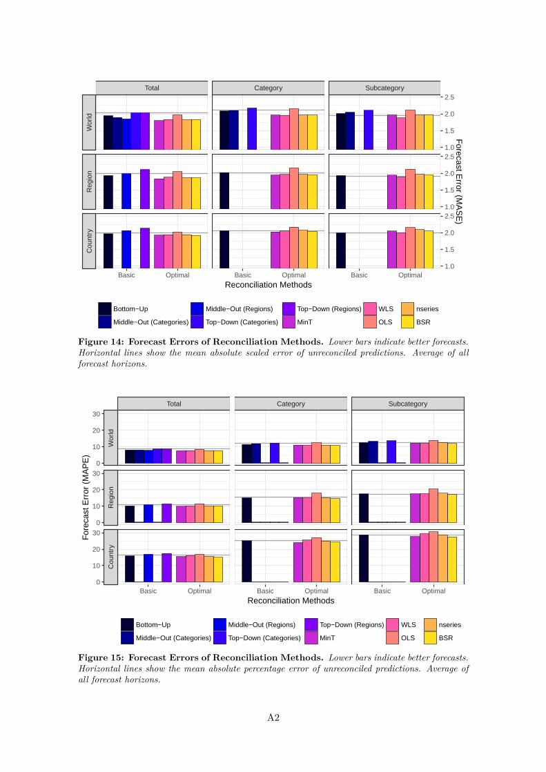
Figure 14: Forecast Errors of Reconciliation Methods. Lower bars indicate better forecasts.Horizontal lines show the mean absolute scaled error of unreconciled predictions. Average of allforecast horizons.
Total Category Subcategory
Wor
ldR
egio
nC
ount
ry
Basic Optimal Basic Optimal Basic Optimal
0
10
20
30
0
10
20
30
0
10
20
30
Reconciliation Methods
For
ecas
t Err
or (
MA
PE
)
Bottom−Up
Middle−Out (Categories)
Middle−Out (Regions)
Top−Down (Categories)
Top−Down (Regions)
MinT
WLS
OLS
nseries
BSR
Figure 15: Forecast Errors of Reconciliation Methods. Lower bars indicate better forecasts.Horizontal lines show the mean absolute percentage error of unreconciled predictions. Average ofall forecast horizons.
A2

A.2 Data
The data is compiled by the Swiss Federal Customs Administration4.
Table 1: Description of Categorical Hierarchy
No. Description01 Forestry and agricultural products, fisheries01.1 Food, beverages and tobacco01.2 Feeding stuffs for animals01.3 Live animals01.4 Horticultural products01.5 Forestry products (not firewood)01.6 Products for commercial/industrial further processing such as oils, fats, starches,
plants and vegetable parts, etc.
02 Energy source02.1 Solid combustibles02.2 Petroleum and distillates02.3 Gas02.4 Electrical energy
03 Textiles, clothing, shoes03.1 Textiles03.2 Articles of apparel and clothing03.3 Shoes, parts and accessories
04 Paper, articles of paper and and products of the printing industry04.1 Basic materials for paper production, such as cellulose and cellulose fibre and paper
and carton waste04.2 Paper and carton in rolls, strips or sheets04.3 Goods from paper or carton04.4 Products of the printing industry
05 Leather, rubber, plastics05.1 Leather05.2 Rubber05.3 Plastics
06 Products of the chemical and pharmaceutical industry06.1 Chemical raw materials, basic materials and unformed plastics06.2 Chemical end products, vitamins, diagnostic products, including active substances
07 Stones and earth07.1 Mineral raw materials and basic products07.2 Goods from stone and cement07.3 Ceramic wares07.4 Glass
08 Metals08.1 Iron and steel08.2 Non-ferrous metals
continued . . .
4https://www.ezv.admin.ch/ezv/en/home/topics/swiss-foreign-trade-statistics.html
A3

. . . continued
08.3 Metal goods
09 Machines, appliances, electronics09.1 Industrial machinery09.2 Agricultural machines09.3 Household appliances09.4 Office machines09.5 Electrical and electronic industry appliances and devices09.6 Military equipment
10 Vehicles10.1 Road vehicles10.2 Railed vehicles10.3 Air- and spacecraft10.4 Watercraft
11 Precision instruments, clocks and watches and jewellery11.1 Precision instruments and equipment11.2 Watches11.3 Jewellery and household goods made from precious metals
12 Various goods such as music instruments, home furnishings, toys, sports equipment,etc.
12.1 Exposed film12.2 Music instruments12.3 Home furnishings12.4 Toys and sports equipment12.5 Stationery goods12.6 Various goods such as umbrellas, neon signs, festive articles, brushes, lighters, pipes,
etc.
13 Precious metals, precious and semi-precious stones13.1 Precious and semi-precious stones13.2 Precious metals (including gold and silver bars from 1.1.2012)
14 Works of art and antiques14.1 Works of art14.2 Antiques and collectors’ items
Table 2: Description of Geographical Hierarchy
Country valid from valid to
EuropeDE Germany 01/1988 -FR France 01/1988 -IT Italy 01/1988 -NL Netherlands 01/1988 -BE Belgium-Luxembourg 01/1988 12/1998BE Belgium 01/1999 -LU Luxembourg 01/1999 -AT Austria 01/1988 -
continued . . .
A4

. . . continued
GB United Kingdom 01/1988 -DK Denmark 01/1988 -NO Norway 01/1988 -SE Sweden 01/1988 -PT Portugal 01/1988 -FI Finland 01/1988 -HR Croatia, Republic of 02/1992 -SI Slovenia 02/1992 -BA Bosnia and Herzegovina 05/1992 -MK North Macedonia 05/1992 -ME Montenegro 05/1992 12/1996ME Montenegro 01/2007 -XM Montenegro 01/2006 12/2006SQ Serbia 05/1992 12/1996RS Serbia 01/2007 -XS Serbia 01/2006 12/2006YU Federal Republic of Yugoslavia 01/1997 12/2003CS Serbia and Montenegro 01/2004 12/2005XK Kosovo 01/2006 -IS Iceland 01/1988 -IE Ireland 01/1988 -ES Spain 01/1988 -GR Greece 01/1988 -TR Turkey 01/1988 -DD GDR 01/1988 10/1990PL Poland 01/1988 -CZ Czech Republic 01/1993 -CS Czechoslovakia 01/1988 02/1992SK Slovakia 01/1993 -HU Hungary 01/1988 -AL Albania 01/1988 -BG Bulgaria, Republic of 01/1988 -RO Romania 01/1988 -SU USSR 01/1988 12/1991YU Yugoslavia 01/1988 04/1992CY Cyprus 01/1988 -SJ Svalbard and Jan Mayen Island 01/1999 -MT Malta 01/1988 -GI Gibraltar 01/1988 -FO Faeroe Islands 01/1988 -SM San Marino 01/1999 -VA Holy See 01/1999 -AD Andorra 01/1988 -EE Estonia 01/1992 -LV Latvia 01/1992 -LT Lithuania 01/1992 -QX Countries not specified 01/2002 -
Central Asia
continued . . .
A5

. . . continued
RU Russian Federation 01/1992 -AM Armenia 01/1992 -AZ Azerbaijan 01/1992 -BY Belarus 01/1992 -GE Georgia 01/1992 -KZ Kazakhstan 01/1992 -KG Kyrgyz, Republic 01/1992 -MD Moldova, Republic of 01/1992 -TJ Tajikistan 01/1992 -TM Turkmenistan 01/1992 -UA Ukraine 01/1992 -UZ Uzbekistan 01/1992 -
Africa and Middle EastEG Egypt 01/1988 -SD Sudan 01/1988 -SS South Sudan, Republic of 09/2011 -LY Libya 01/1988 -TN Tunisia 01/1988 -DZ Algeria 01/1988 -XA Canary Islands 01/1988 -MA Morocco 01/1988 -EH Western Sahara 01/1999 -XB Ceuta and Melilla 01/1988 12/2010GQ Equatorial Guinea 01/1988 -XC Ceuta 01/2001 -XL Melilla 01/2001 -TG Togo 01/1988 -SN Senegal 01/1988 -ML Mali 01/1988 -MR Mauritania 01/1988 -CI Côte d’Ivoire 01/1988 -BF Burkina Faso 01/1988 -BJ Benin 01/1988 -NE Niger 01/1988 -GN Guinea 01/1988 -GM Gambia 01/1988 -SL Sierra Leone 01/1988 -LR Liberia 01/1988 -GH Ghana 01/1988 -NG Nigeria, Federal Republic of 01/1988 -CM Cameroon 01/1988 -GA Gabon 01/1988 -CG Congo, Republic of the 01/1988 -CF Central African Republic 01/1988 -TD Chad 01/1988 -CD Congo, Democratic Republic of the 06/1997 -ZR Zaire 01/1988 05/1997AO Angola 01/1988 -
continued . . .
A6

. . . continued
GW Guinea-Bissau 01/1988 -BW Botswana 01/1988 -CV Cabo Verde, Republic of 01/1988 -LS Lesotho 01/1988 -ST Sao Tomé and Principe 01/1988 -NA Namibia 01/1988 -ZA South Africa 01/1988 -SZ Swaziland 01/1988 -ZM Zambia 01/1988 -ZW Zimbabwe 01/1988 -MW Malawi 01/1988 -MZ Mozambique 01/1988 -MG Madagascar, Republic of 01/1988 -RE RÈunion 01/1988 -SH St Helena, Ascen. and Tristan da Cunha 01/1988 -KM Comoros, Union of 01/1988 -AQ Antarctica 01/1988 -MU Mauritius 01/1988 -IO British Indian Ocean Territory 01/1988 -TZ Tanzania, United Republic of 01/1988 -SC Seychelles, Republic of 01/1988 -RW Rwanda 01/1988 -BV Bouvet Island 01/1999 -BI Burundi 01/1988 -YT Mayotte 01/1999 -SO Somalia, Federal Republic of 01/1988 -TF French Southern Territories 01/1999 -DJ Djibouti 01/1988 -ER Eritrea 01/1994 -ET Ethiopia, Fed. Democratic Republic of 01/1988 -KE Kenya 01/1988 -UG Uganda 01/1988 -SY Syrian Arab Republic 01/1988 -LB Lebanon 01/1988 -IL Israel 01/1988 -PS Palestine, the State of 01/1997 -JO Jordan 01/1988 -SA Saudi Arabia 01/1988 -YE Yemen (Nord) 01/1988 12/1990YE Yemen 01/1991 -YD Yemen (Sud) 01/1988 12/1990QA Qatar 01/1988 -BH Bahrain 01/1988 -AE United Arab Emirates 01/1988 -OM Oman 01/1988 -KW Kuwait 01/1988 -IQ Iraq 01/1988 -IR Iran, Islamic Republic of 01/1988 -
continued . . .
A7

. . . continued
South AsiaAF Afghanistan 01/1988 -PK Pakistan 01/1988 -BD Bangladesh 01/1988 -IN India 01/1988 -LK Sri Lanka 01/1988 -MV Maldives 01/1988 -NP Nepal, Federal Democratic Rep. 01/1988 -BT Bhutan 01/1988 -
East AsiaMM Myanmar, Union of 01/1988 -TH Thailand 01/1988 -MY Malaysia 01/1988 -BN Brunei Darussalam 01/1988 -SG Singapore 01/1988 -KH Cambodia 01/1988 -LA Lao, People’s Democratic Republic 01/1988 -VN Viet Nam, Socialist Republic of 01/1988 -MN Mongolia 01/1988 -CN China, People’s Republic of 01/1988 -HK Hong Kong 01/1988 -TW Taiwan 01/1988 -MO Macau 01/1988 -KP Korea, People’s Democratic Republic of 01/1988 -KR Korea, Republic of 01/1988 -JP Japan 01/1988 -PH Philippines 01/1988 -ID Indonesia 01/1988 -TL East Timor 01/2004 -TP East Timor 01/1999 12/2003
North AmericaCA Canada 01/1988 -PM St Pierre and Miquelon 01/1988 -US United States 01/1988 -GL Greenland 01/1988 -
Latin AmericaMX Mexico 01/1988 -BZ Belize 01/1988 -GT Guatemala 01/1988 -HN Honduras 01/1988 -SV El Salvador 01/1988 -NI Nicaragua 01/1988 -CR Costa Rica 01/1988 -PA Panama 01/1988 -KY Cayman Islands 01/1988 -TC Turks and Caicos Islands 01/1988 -BS Bahamas 01/1988 -
continued . . .
A8

. . . continued
BM Bermuda 01/1988 -JM Jamaica 01/1988 -CU Cuba 01/1988 -HT Haiti 01/1988 -DO Dominican Republic 01/1988 -VI American Virgin Islands 01/1988 -PR Puerto Rico 01/1988 12/2005DM Dominica 01/1988 -VC St Vincent and the Grenadines 01/1988 -LC St Lucia 01/1988 -MS Montserrat 01/1988 -AG Antigua and Barbuda 01/1988 -BB Barbados 01/1988 -GD Grenada 01/1988 -KN St Kitts and Nevis 01/1988 -AI Anguilla 01/1988 -GP Guadeloupe 01/1988 -VG British Virgin Islands 01/1999 -MQ Martinique 01/1988 -TT Trinidad and Tobago 01/1988 -BL Saint BarthÈlemy 01/2013 -AN Netherlands Antilles 01/1988 12/2012AW Aruba 01/1999 -BQ Bonaire, Sint Eustatius and Saba 01/2013 -CW Curacao 01/2013 -SX Sint Maarten (NL) 01/2013 -CO Colombia 01/1988 -VE Venezuela, the Bolivarian Republic of 01/1988 -GY Guyana 01/1988 -SR Suriname 01/1988 -GF French Guiana 01/1988 -BR Brazil 01/1988 -PY Paraguay 01/1988 -UY Uruguay 01/1988 -AR Argentina 01/1988 -FK Falkland Islands 01/1988 -GS South Georgia and South Sandwich Islands 01/1999 -CL Chile 01/1988 -BO Bolivia, the Plurinational State of 01/1988 -PE Peru 01/1988 -EC Ecuador 01/1988 -
Australia and OceaniaAU Australia 01/1988 -PG Papua New Guinea 01/1988 -CC Cocos (Keeling) Islands 01/1999 -HM Heard and McDonald Islands 01/1999 -NF Norfolk Island 01/1999 -CX Christmas Island 01/1999 -
continued . . .
A9

. . . continued
NZ New Zealand 01/1988 -CK Cook Islands 01/1998 -WS Samoa 01/1988 -NU Niue Island 01/1999 -KI Kiribati, the Republic of 01/1988 -TK Tokelau Islands 01/1999 -TV Tuvalu 01/1988 -PN Pitcairn Islands 01/1988 -SB Solomon Islands 01/1988 -PF French Polynesia 01/1988 -NC New Caledonia 01/1999 -WF Wallis and Futuna 01/1999 -PU American Oceania 01/1988 12/1996UM American Oceania 01/2006 -UM American Oceania 01/1997 12/2005MP Northern Mariana, Islands 01/1997 -MH Marshall Islands 01/1997 -FM Micronesia, Federated States of 01/1997 -PW Palau 01/1997 -FJ Fiji, Republic of 01/1988 -AS American Samoa 01/2006 -GU Guam 01/2006 -VU Vanuatu 01/1988 -NR Nauru 01/1988 -TO Tonga 01/1988 -
A10