Automatic Horizon Picking in 3D Seismic Data Using Optical Filters and Minimum Spanning Tree(Patent Pending)Yingwei Yu*, Cliff Kelley, and Irina Mardanova, Seismic Micro-Technology, Inc.

SUMMARY

Horizon picking in 3D seismic data is a very challenging prob-

lem. The difficulty for automatic horizon extraction exists at

least in two fold: (1) the selection of picks in a trace usu-

ally ignores lateral continuity, and (2) the trace traversal or-

der can result in significantly different horizons so that the

resulting picks in the same horizon often conflict with each

other. In this paper, a pattern recognition-based algorithm is

presented to explicitly address these two difficulties: (1) se-

lect a pick within a trace by considering context information

through orientation filters which help to preserve the lateral

continuity among traces; (2) perform the trace selection us-

ing the minimum-spanning tree (MST) algorithm based on the

confidence maximum at each pick. Combining the pick se-

lection and trace selection components together allows us to

obtain highly accurate horizon surfaces.

INTRODUCTION

A horizon is characterized by seismic reflection properties in a

depositional environment and can be represented as a three di-

mensional surface between rock layers (Faraklioti and Petrou,

2004). The goal of the horizon auto-picking is to track a user

selected phase of the horizon curve waveform automatically

by a computer algorithm. The design of the 3D horizon auto-

picking algorithm must deal with the following problems:

• Trace selection: Automatically decide the trace traver-

sal order to apply the pick selection. It has the follow-

ing two properties: (a) Completeness. For any two

picks, if they are connected, either directly or through

other picks, we say they are in the same horizon seg-

ment. The trace selection should traverse all the ac-

cessible picks in the same horizon segments to make

it complete. For some data, such as a salt dome, a

conventional line-by-line trace selection method is in-

complete and fails to traverse the portion across the

dome. (b) Traversal order dependency. The resulting

horizon can appear significantly different if the traces

are traversed in a different order in the same survey.

For example, the resulting horizon generated by line-

by-line is quite different to the one by first-in-first-out

(FIFO) method. Moreover, the line-by-line approach

creates incoherent results for complex horizon. That is,

the horizon picks appear very rough and jump across

phase cycles from line to line. Same behavior can be

observed in a FIFO-based picker.

• Pick selection: Find a pick on a given trace. We pro-

pose a pick selection method with the aid of orientation

vectors calculated for seismic data. Orientation vectors

in 3D space can be derived from 2D vectors calculated

along the inline and crossline directions.

These properties greatly complicate horizon autopicking in 3D,

and often result in the necessity for experienced interpretors to

manually interpret, which is a labor and time intensive pro-

cess. Our solution is to use orientation vectors to accomplish

the above difficulties by the following:

• guide pick selection and optimize the trace selection

by calculating a confidence score between two picks in

neighboring traces, and

• find a complete horizon with maximum overall confi-

dence scores.

AUTOPICKING METHOD

In this section, we first introduce the pick selection algorithm

using an orientation vector field (OVF), and then explain how

the minimum-spanning tree (MST) algorithm (Boruvka, 1926;

Nesetril et al., 2001) is used for the optimized trace selection.

Pick Selection Using Orientation Vector Field

As observed by Harrigan et al. (1992), horizons generally have

a consistently high amplitude reflection signature, and display

some degree of lateral continuity. In the practice of horizon

picking, conventional methods usually employ a window-based

approach in searching extrema. The window-based approach

only looks at the adjacent trace vertically within a time win-

dow, while the lateral continuity is ignored. Its very limited

context often incurs the “off-cycle” effect where the extrema

points are incorrectly linked across seismic phase cycles, which

yield a wrong resulting horizon. This effect can be more severe

in seismic data with high-angle layering structure.

To preserve the lateral continuity of horizon picking, we need

to examine the seismic data patterns in a range of neighbor-

hoods. The context information reveals which direction the

horizon trends. The lateral continuity in 3D can be analyzed by

finding horizon curves in 2D vertical slices, in both inline and

crossline directions. For each seismic image in 2D, the horizon

trends (or the tangent of horizon curves) are the salient contin-

uous features that can be detected visually. Hence filters can

be applied to extract the structural features, i.e., the orientation

vectors, which preserve the lateral continuity.

In the following, we outline a method of using a bank of opti-

cal filters to generate an OVF from a 2D seismic image. The

orientation vector is used to post a new pick on each selected

trace. (The detailed definition of the orientation filters and the

deriving process is patent pending).

To generate the orientation vectors, we first create an array of

optical filters in the frequency domain, and then apply it to the

seismic image to convert the image to the spatial domain. We

2

convolve the seismic image with each filter in the filter bank

iteratively. For the ith filter, the response seismic image can

be represented in the complex space by a real part Yr(x,y) and

an imaginary part Yim(x,y), where x is the trace index, and y

the sample index. The norm of the complex image is called

orientation energy (OE):

Y i(x,y) =√

[Y ir (x,y)]

2 +[Y iim(x,y)]

2.

The maximum response of all filters at a particular sample

point (x,y) is the value of the orientation energies:

E(x,y) = maxi(Y i(x,y))

The orientation energy E reflects the strength of orientation

features at each point, while the filter index i of the maximum

response defines the orientation angle γ at each point (x,y),which forms the orientation vector field (OVF). The orienta-

tion energy can be used as a stopping criteria for horizon pick-

ing. Low values of orientation energy means that the structure

feature is less oriented, while stronger value means the orien-

tation feature is more salient in the context. In an area with less

of structure features, such as the interior of the salt dome, the

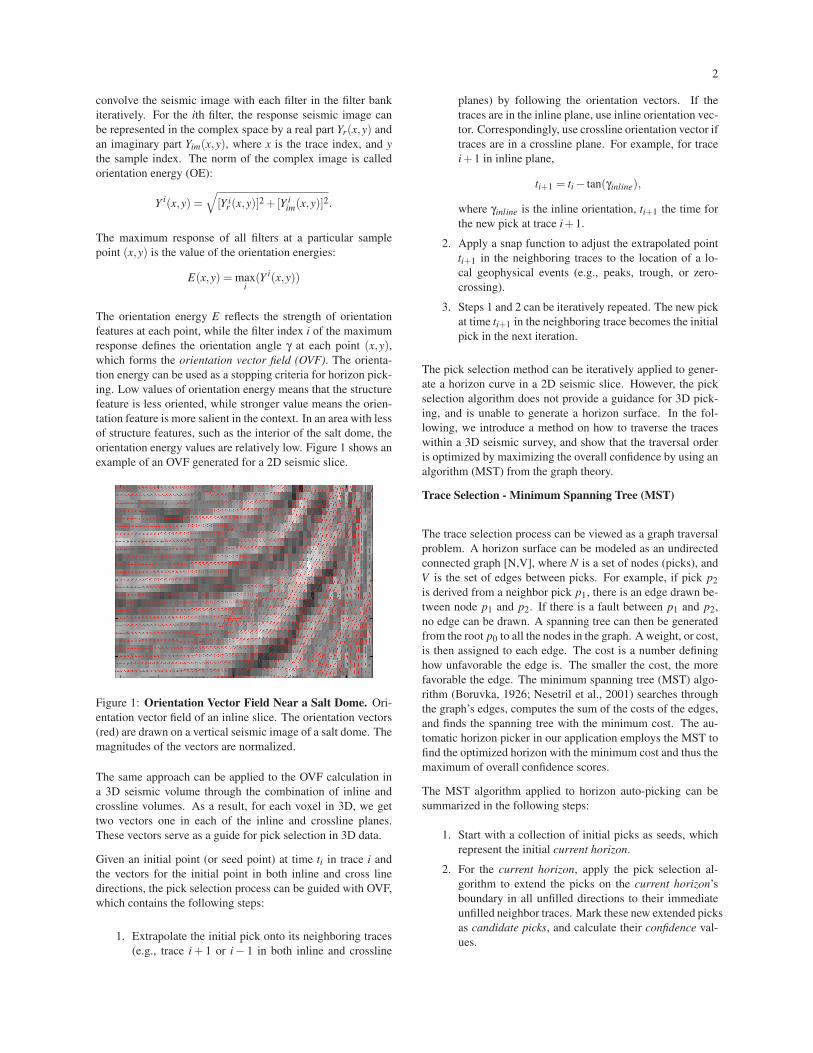
orientation energy values are relatively low. Figure 1 shows an

example of an OVF generated for a 2D seismic slice.

Figure 1: Orientation Vector Field Near a Salt Dome. Ori-

entation vector field of an inline slice. The orientation vectors

(red) are drawn on a vertical seismic image of a salt dome. The

magnitudes of the vectors are normalized.

The same approach can be applied to the OVF calculation in

a 3D seismic volume through the combination of inline and

crossline volumes. As a result, for each voxel in 3D, we get

two vectors one in each of the inline and crossline planes.

These vectors serve as a guide for pick selection in 3D data.

Given an initial point (or seed point) at time ti in trace i and

the vectors for the initial point in both inline and cross line

directions, the pick selection process can be guided with OVF,

which contains the following steps:

1. Extrapolate the initial pick onto its neighboring traces

(e.g., trace i+ 1 or i− 1 in both inline and crossline

planes) by following the orientation vectors. If the

traces are in the inline plane, use inline orientation vec-

tor. Correspondingly, use crossline orientation vector if

traces are in a crossline plane. For example, for trace

i+1 in inline plane,

ti+1 = ti − tan(γinline),

where γinline is the inline orientation, ti+1 the time for

the new pick at trace i+1.

2. Apply a snap function to adjust the extrapolated point

ti+1 in the neighboring traces to the location of a lo-

cal geophysical events (e.g., peaks, trough, or zero-

crossing).

3. Steps 1 and 2 can be iteratively repeated. The new pick

at time ti+1 in the neighboring trace becomes the initial

pick in the next iteration.

The pick selection method can be iteratively applied to gener-

ate a horizon curve in a 2D seismic slice. However, the pick

selection algorithm does not provide a guidance for 3D pick-

ing, and is unable to generate a horizon surface. In the fol-

lowing, we introduce a method on how to traverse the traces

within a 3D seismic survey, and show that the traversal order

is optimized by maximizing the overall confidence by using an

algorithm (MST) from the graph theory.

Trace Selection - Minimum Spanning Tree (MST)

The trace selection process can be viewed as a graph traversal

problem. A horizon surface can be modeled as an undirected

connected graph [N,V], where N is a set of nodes (picks), and

V is the set of edges between picks. For example, if pick p2

is derived from a neighbor pick p1, there is an edge drawn be-

tween node p1 and p2. If there is a fault between p1 and p2,

no edge can be drawn. A spanning tree can then be generated

from the root p0 to all the nodes in the graph. A weight, or cost,

is then assigned to each edge. The cost is a number defining

how unfavorable the edge is. The smaller the cost, the more

favorable the edge. The minimum spanning tree (MST) algo-

rithm (Boruvka, 1926; Nesetril et al., 2001) searches through

the graph’s edges, computes the sum of the costs of the edges,

and finds the spanning tree with the minimum cost. The au-

tomatic horizon picker in our application employs the MST to

find the optimized horizon with the minimum cost and thus the

maximum of overall confidence scores.

The MST algorithm applied to horizon auto-picking can be

summarized in the following steps:

1. Start with a collection of initial picks as seeds, which

represent the initial current horizon.

2. For the current horizon, apply the pick selection al-

gorithm to extend the picks on the current horizon’s

boundary in all unfilled directions to their immediate

unfilled neighbor traces. Mark these new extended picks

as candidate picks, and calculate their confidence val-

ues.

3

3. Select the candidate pick with the maximum confidence

among all the candidate picks.

4. Add the candidate pick into the current horizon, and

the candidate pick becomes a confirmed pick in the cur-

rent horizon.

5. Repeat steps 2 to 4 until no new pick can be added. The

result is the final horizon.

The confidence function is a heuristic function to guide the

search for MST, which is discussed in the next section.

Confidence Factors

Given two neighboring traces i and j, and two sample points

with sample indice p and q on each trace, we can estimate the

possibility of these two points belonging to the same horizon

by the following criteria:

• Pattern of the picks and their context: Let P be the

amplitude vector around the candidate pick p within a

guide window, and Q be the amplitude vector around

the pick q within the same guide window. Define the

curve pattern similarity χ as the correlation coefficient

between the amplitude vectors P and Q.

• Vertical locations of the picks: When the horizon is

flat and smooth, the average vertical difference between

picks is just a small amount, therefore the probability

of these picks belonging to the same horizon is high.

The difference value ρ can be defined as:

ρ = avgq∈Neighbors(p)(|p−q|)

With the above analysis, we combine both factors into one con-

fidence value, c, for the candidate pick p and its predecessor

pick q using the equation below:

c(p,q) = χe−kρ,

where k is a user-defined constant (e.g., 0.5) to control the sen-

sitivity to the vertical shift factor. The candidate pick’s con-

fidence value is between 0 and 1. During the horizon pick-

ing process, the horizon’s confidence attribute is generated and

saved.

EXAMPLE

The described algorithm was tested on a 3D Salt Dome survey

(courtesy of FairfieldNodal). The data is characterized by a

large number of faults and one big salt dome in the center. To

verify the robustness and accuracy of our algorithm, the fault

surfaces were not picked prior to the horizon interpretation.

OVF for both inline and crossline planes are calculated before

the autopicking starts. Each voxel in the seismic data contains

two orientation vectors, one along the inline direction, and the

other along the crossline direction. Figure 1 shows the orienta-

tion vectors generated in one vertical slice display along inline

direction across the salt dome.

After generating the orientation vectors, we applied the MST

algorithm to search for the horizon picks in 3D. Figure 2 shows

(a) Horizon in Vertical Slice Display View

(b) A Salt Dome Horizon in Base Map View

(c) Confidence in Base Map View

Figure 2: A Salt Dome Horizon. (a) The vertical line in this

display is located at the north side of the dome. Note that

the horizon segments (green) are automatically matched across

uninterpreted faults. (b) In the basemap view of horizon, the

fault is automatically outlined by picking the points with high

confidence in the surrounding. (c) The confidence values are

high in flat and clean areas, but low around the faults and salt

dome. The confidence values are used to prioritize the candi-

date picks in the queue during the picking process.

the resulting horizon rendered on a vertical slice (a) and a base

map (b). Note that the faults over the horizon are automati-

4

cally detected by sorting the confidence of candidate picks (see

confidence results in Figure 2c), and fault patterns are formed

naturally by picking high confidence picks first in the fault sur-

roundings, leaving the fault area with very low or zero confi-

dence. As shown in the Figure 2a, the four horizon segments

are correctly picked across several uninterpreted faults. These

four horizon segments appear discontinuous in 2D view; how-

ever, they actually connect to each other in 3D view. This ver-

tical line is located on the north side of the salt dome. The

confidence values are also low at locations around the dome,

and is why the picking process stops without going into the

dome area.

CONCLUSIONS

This paper introduced a pattern recognition-based horizon pick-

ing method which contains two components: an orientation

vector guided search for pick selection in a trace, and an MST-

based search for trace selection. Besides the application in

horizon autopicking, the OVF may have many potential appli-

cations in seismic interpretation, such as volumetric curvature

calculation. The second component, trace selection MST, is an

optimized method to traverse the horizon coherently. Combin-

ing these two components of filter array and MST, the intro-

duced horizon picking algorithm is an effective way to pick a

coherent horizon in 3D seismic data thoroughly and accurately.

The proposed horizon auto-picking algorithm can significantly

reduce the costs and improve the quality for automatic horizon

interpretation.

ACKNOWLEDGMENTS

The authors would like to thank FairfieldNodal for permis-

sion to show the results using the salt dome data. Thanks to

Michael McCormack, Gary Jones, Stan Abele, Rocky Roden,

Ramoj Paruchuri, Robert Baker, Christopher Lewis, and Hai

Xu for many helpful discussions, and Sandra Rimmer for the

help with editing.

EDITED REFERENCES

Note: This reference list is a copy-edited version of the reference list submitted by the author. Reference lists for the 2011

SEG Technical Program Expanded Abstracts have been copy edited so that references provided with the online metadata for

each paper will achieve a high degree of linking to cited sources that appear on the Web.

REFERENCES

Borůvka, O., 1926, On a certain minimal problem: Praca Moravske Prirodovedecke Spolecnosti, 3, 37–58

(in Czech).

Faraklioti, M., and M. Petrou, 2004, Horizon picking in 3D seismic data volumes: Machine Vision and

Applications, 15, 216–219, doi:10.1007/s00138-004-0151-8.

Harrigan, E., J. Kroh, W. Sandham, and T. Durrani, 1992, Seismic horizon picking using an artificial

neural network: International Conference on Acoustics, Speech, and Signal Processing, IEEE, 3,

105–108.

Nešetřil, J., E. Milková, and H. Nešetřilová, 2001, Otakar Borůvka on minimum spanning tree problem:

Translation of both the 1926 papers, comments, history: Discrete Mathematics, 233, 3–36.