
Automated statistical forecasting for quality attributes ... · Automated Statistical Forecasting...
261
Automated Statistical Forecasting for Quality Attributes of Web Services Ayman Ahmed Amin Abdellah Submitted in fulfilment of the requirements of the degree of Doctor of Philosophy Faculty of Science, Engineering and Technology Swinburne University of Technology Coordinating Supervisors: Dr. Alan Colman, Swinburne University of Technology, Australia Prof. Lars Grunske, University of Stuttgart, Germany 2014
Transcript of Automated statistical forecasting for quality attributes ... · Automated Statistical Forecasting...

Automated Statistical Forecasting for
Quality Attributes of Web Services
Ayman Ahmed Amin Abdellah
Submitted in fulfilment of the requirements
of the degree of Doctor of Philosophy
Faculty of Science, Engineering and Technology
Swinburne University of Technology
Coordinating Supervisors:
Dr. Alan Colman, Swinburne University of Technology, Australia
Prof. Lars Grunske, University of Stuttgart, Germany
2014


Abstract
Web services provide a standardized solution for service-oriented architecture. Con-
sumers of such services expect they will meet quality of service (QoS) attributes
such as performance. Monitoring such QoS attributes is necessary to ensure con-
formance to requirements. However, the reactive detection of past QoS violations
can lead to critical problems as the violation has already occurred and consequent
costs may be unavoidable. To address these problems, researchers have proposed
approaches to proactively detect potential violations using time series modeling. In
this thesis, these approaches are reviewed and their limitations are highlighted. One
of the main challenges of effective time series forecasting of diverse Web services is
that their stochastic behavior needs to be characterized before adequate time se-
ries models can be derived. Furthermore, given the continuously changing nature
of service provisioning and demand, the adequacy and forecasting accuracy of the
constructed time series models need to be continuously evaluated at runtime.
In this thesis, these challenges are addressed, and the outcome is a collection
of QoS characteristic-specific automated forecasting approaches. Each one of these
approaches is able to fit and forecast only a specific type of QoS stochastic character-
istics, however, taken together they will be able to fit different dynamic behaviors of
QoS attributes and forecast their future values. In particular, the thesis proposes an
automated forecasting approach for nonlinearly dependent QoS attributes, two auto-
mated forecasting approaches for linearly dependent QoS attributes with volatility
clustering (i.e. nonstationary variance over time), and two automated forecast-
ing approaches for nonlinearly dependent QoS attributes with volatility clustering.
These forecasting approaches provide the basis for a general automated forecasting
approach for QoS attributes. The accuracy and performance of the proposed fore-
casting approaches are evaluated and compared to those of the baseline ARIMA
time series models using real-world QoS datasets of Web services characterized by
nonlinearity and volatility clustering. The evaluation results show that each one of
the proposed forecasting approaches outperforms the baseline ARIMA models.
i

ii

Acknowledgements
My sincere thanks to my supervisors Prof. Lars Grunske and Dr Alan Colman for
their generous mentoring and many hours spent discussing the topics and reviewing
papers and thesis drafts. My thanks also go to fellow PhD students Mahmoud,
Khaled, Sayed, Iman, Tharindu, Indika, Ashad, and Kaw for making a friendly and
enjoyable research student life.
I would like to express my profound gratitude to my whole family who always
gave their fullest support, care, and encouragement to make this research a success.
iii

iv

Declaration
This thesis contains no material which has been accepted for the award of any other
degree or diploma, except where due reference is made in the text of the thesis. To
the best of my knowledge, this thesis contains no material previously published or
written by another person except where due reference is made in the text of the
thesis.
Ayman Ahmed Amin Abdellah
v

vi

List of Publications
The following papers have been accepted and published during my candidature. The
thesis is largely based on these papers.
• Ayman Amin, Lars Grunske, and Alan Colman, “An Approach to Software
Reliability Prediction based on Time Series Modeling,” The Journal of Systems
and Software, Volume 86, Issue 7, Pages 1923–1932, 2013.
• Ayman Amin, Lars Grunske, and Alan Colman, “An Automated Approach
to Forecasting QoS Attributes Based on Linear and Non-linear Time Series
Modeling,” in proceedings of the 27th IEEE/ACM International Conference
on Automated Software Engineering (ASE), Germany. IEEE/ACM, 2012.
• Ayman Amin, Alan Colman, and Lars Grunske, “An Approach to Forecast-
ing QoS Attributes of Web Services Based on ARIMA and GARCH Models,”
in proceedings of the 19th IEEE International Conference on Web Services
(ICWS), USA. IEEE, 2012.
• Indika Meedeniya, Aldeida Aleti, Iman Avazpour and Ayman Amin, “Ro-
bust ArcheOpterix: Architecture Optimization of Embedded Systems Under
Uncertainty,” in proceedings of the 2nd International ICSE Workshop on Soft-
ware Engineering for Embedded Systems (SEES), Switzerland. IEEE, 2012.
• Ayman Amin, Alan Colman, and Lars Grunske, “Statistical Detection of
QoS Violations Based on CUSUM Control Charts,” in proceedings of the 3rd
ACM/SPEC International Conference on Performance Engineering (ICPE),
USA. ACM, 2012.
• Ayman Amin, Alan Colman, and Lars Grunske, “Using Automated Con-
trol Charts for the Runtime Evaluation of QoS Attributes,” in proceedings of
the 13th IEEE International High Assurance Systems Engineering Symposium
(HASE), USA. IEEE, 2011.
vii

viii
Contents
Abstract i
Acknowledgements iii
Declaration v
List of Publications vii
Abbreviations xxiii
1 Introduction 1
Existing Approaches and Limitations in a Nutshell . . . . . . . . . . . . . 2
Research Problem . . . . . . . . . . . . . . . . . . . . . . . . . . . . . . . . 4
Overview of Research Method . . . . . . . . . . . . . . . . . . . . . . . . . 6
Scope of the Research . . . . . . . . . . . . . . . . . . . . . . . . . . . . . 8
Contributions . . . . . . . . . . . . . . . . . . . . . . . . . . . . . . . . . . 8
Thesis Outline . . . . . . . . . . . . . . . . . . . . . . . . . . . . . . . . . 10
2 Background and Related Work 13
2.1 Background . . . . . . . . . . . . . . . . . . . . . . . . . . . . . . . . 13
2.1.1 Web Services, Composition, and Service-Based Systems . . . . 14
2.1.2 Quality of Service Attributes . . . . . . . . . . . . . . . . . . . 16
2.1.2.1 QoS Attributes Definition and Classification . . . . . 17
2.1.2.2 Monitoring Approaches for QoS Attributes . . . . . . 21
ix

CONTENTS
2.1.2.3 Importance of Using QoS Attributes in Web Services 22
2.2 Review of Related Work . . . . . . . . . . . . . . . . . . . . . . . . . 24
2.2.1 Existing Approaches for Reactive Detection of QoS Violations 25
2.2.1.1 Threshold Based Approaches . . . . . . . . . . . . . 25
2.2.1.2 Statistical Methods Based Approaches . . . . . . . . 28
2.2.1.3 Summary and Limitations of Reactive Approaches . 32
2.2.2 Existing Approaches for Proactive Detection of QoS Violations 35
2.2.2.1 Existing Approaches Based on Time Series Modeling 40
2.2.2.2 Summary and Limitations of Time Series Modeling
Based Approaches . . . . . . . . . . . . . . . . . . . 42
2.3 Summary . . . . . . . . . . . . . . . . . . . . . . . . . . . . . . . . . 46
3 Research Methodology 47
3.1 Research Questions . . . . . . . . . . . . . . . . . . . . . . . . . . . . 48
3.2 Research Approach and Solution . . . . . . . . . . . . . . . . . . . . . 49
3.2.1 Evaluating Stochastic Characteristics of QoS Attributes . . . . 50
3.2.2 Specifying Class of Adequate Time Series Models . . . . . . . 52
3.2.3 Constructing Adequate Time Series Models . . . . . . . . . . 53
3.2.4 Evaluating Adequacy and Forecasting Accuracy . . . . . . . . 56
3.2.5 Expected Outcome of Addressing Research Questions . . . . . 59
3.3 Evaluation Strategy . . . . . . . . . . . . . . . . . . . . . . . . . . . . 59
3.4 Summary . . . . . . . . . . . . . . . . . . . . . . . . . . . . . . . . . 63
4 Evaluation of Stochastic Characteristics of QoS Attributes 65
4.1 Invocation of Real-World Web Services . . . . . . . . . . . . . . . . . 66
4.2 QoS Stochastic Characteristics and How to Evaluate . . . . . . . . . 70
4.2.1 Probability Distribution and Transformation to Normality . . 72
4.2.2 Serial Dependency . . . . . . . . . . . . . . . . . . . . . . . . 78
4.2.3 Stationarity . . . . . . . . . . . . . . . . . . . . . . . . . . . . 80
4.2.3.1 Stationarity in the Mean . . . . . . . . . . . . . . . . 81
x

CONTENTS
4.2.3.2 Stationarity in the Variance . . . . . . . . . . . . . . 82
4.2.4 Nonlinearity . . . . . . . . . . . . . . . . . . . . . . . . . . . . 86
4.3 Results of Evaluating QoS Stochastic Characteristics . . . . . . . . . 87
4.4 Summary . . . . . . . . . . . . . . . . . . . . . . . . . . . . . . . . . 91
5 Forecasting Approach for Nonlinearly Dependent QoS Attributes 93
5.1 Background of Time Series Models . . . . . . . . . . . . . . . . . . . 94
5.1.1 ARIMA Models . . . . . . . . . . . . . . . . . . . . . . . . . . 94
5.1.2 Bilinear Time Series Models . . . . . . . . . . . . . . . . . . . 95
5.1.3 Exponential Autoregressive Time Series Models . . . . . . . . 96
5.1.4 SETARMA Models . . . . . . . . . . . . . . . . . . . . . . . . 97
5.1.5 Assumptions of Time Series Models . . . . . . . . . . . . . . . 99
5.2 Forecasting Approach I based on SETARMA Models . . . . . . . . . 100
5.2.1 SETARMA Model Construction Process . . . . . . . . . . . . 101
5.2.1.1 (P1) Data Preparation . . . . . . . . . . . . . . . . . 101
5.2.1.2 (P2) Initial Model Order Identification . . . . . . . . 102
5.2.1.3 (P3) Delay Parameter and Thresholds Identification 104
5.2.1.4 (P4) Adequate Models Specification . . . . . . . . . 105
5.2.1.5 (P5) Models Estimation . . . . . . . . . . . . . . . . 106
5.2.1.6 (P6) Models Checking and the Best Model Selection 107
5.2.2 Continuously Forecasting Process . . . . . . . . . . . . . . . . 111
5.2.2.1 (P7) Computing Forecasts and Predictive Residuals . 111
5.2.2.2 (P8) Evaluating Adequacy and Forecasting Accuracy 111
5.3 Summary . . . . . . . . . . . . . . . . . . . . . . . . . . . . . . . . . 115
6 Forecasting Approaches for Linearly Dependent QoS Attributes
with Volatility Clustering 117
6.1 Background of GARCH Models and Wavelet Analysis . . . . . . . . . 119
6.1.1 GARCH Models . . . . . . . . . . . . . . . . . . . . . . . . . . 119
6.1.2 Wavelet Analysis . . . . . . . . . . . . . . . . . . . . . . . . . 120
xi

CONTENTS
6.2 Forecasting Approach II Based on ARIMA and GARCH Models . . . 121
6.2.1 ARIMA Model Construction Process . . . . . . . . . . . . . . 121
6.2.1.1 (P1) Data Preparation . . . . . . . . . . . . . . . . . 122
6.2.1.2 (P2) Adequate Models Specification . . . . . . . . . 123
6.2.1.3 (P3) Models Estimation . . . . . . . . . . . . . . . . 124
6.2.1.4 (P4) Models Checking and the Best Model Selection 126
6.2.2 GARCH Model Construction Process . . . . . . . . . . . . . . 128
6.2.2.1 (P5) Computing Squared Residuals . . . . . . . . . . 128
6.2.2.2 (P6 - P8) Adequate GARCH Model Construction . . 128
6.2.3 Continuously Forecasting Process . . . . . . . . . . . . . . . . 129
6.3 Forecasting Approach III Based on Wavelet Analysis, ARIMA and
GARCH Models . . . . . . . . . . . . . . . . . . . . . . . . . . . . . . 131
6.3.1 Wavelet-Based QoS Time Series Decomposition . . . . . . . . 133
6.3.1.1 (P1) Selecting Wavelet Function . . . . . . . . . . . 134
6.3.1.2 (P2) Estimating Decomposition Coefficients and
Constructing Sub-Series . . . . . . . . . . . . . . . . 135
6.3.2 ARIMA and ARIMA-GARCH Models Construction Process . 136
6.3.2.1 (P3) Constructing ARIMA Model for the General
Trend . . . . . . . . . . . . . . . . . . . . . . . . . . 136
6.3.2.2 (P4) Constructing ARIMA-GARCH Model for the
Noises Component . . . . . . . . . . . . . . . . . . . 139
6.3.3 Continuously Forecasting Process . . . . . . . . . . . . . . . . 142
6.3.3.1 (P5) Computing Forecasts and Predictive Residuals . 142
6.3.3.2 (P6) Evaluating Adequacy and Forecasting Accuracy 143
6.4 Summary . . . . . . . . . . . . . . . . . . . . . . . . . . . . . . . . . 145
7 Forecasting Approaches for Nonlinearly dependent QoS Attributes
with Volatility Clustering 147
7.1 Forecasting Approach IV Based on SETARMA and GARCH Models . 148
7.1.1 SETARMA Model Construction Process . . . . . . . . . . . . 148
xii

CONTENTS
7.1.2 GARCH Model Construction Process . . . . . . . . . . . . . . 151
7.1.3 Continuously Forecasting Process . . . . . . . . . . . . . . . . 154
7.2 Forecasting Approach V Based on Wavelet Analysis, SETARMA and
GARCH Models . . . . . . . . . . . . . . . . . . . . . . . . . . . . . . 155
7.2.1 Wavelet-Based QoS Time Series Decomposition . . . . . . . . 159
7.2.2 SETARMA and SETARMA-GARCH Models Construction
Process . . . . . . . . . . . . . . . . . . . . . . . . . . . . . . 159
7.2.2.1 (P3) Constructing SETARMA Model for the Gen-
eral Trend . . . . . . . . . . . . . . . . . . . . . . . . 159
7.2.2.2 (P4) Constructing SETARMA-GARCH Model for
the Noises Component . . . . . . . . . . . . . . . . . 161
7.2.3 Continuously Forecasting Process . . . . . . . . . . . . . . . . 161
7.3 Summary . . . . . . . . . . . . . . . . . . . . . . . . . . . . . . . . . 165
8 Experimental Evaluation 167
8.1 Experiment Setup . . . . . . . . . . . . . . . . . . . . . . . . . . . . . 167
8.2 Results . . . . . . . . . . . . . . . . . . . . . . . . . . . . . . . . . . . 170
8.2.1 EQ1. Improving Forecasting Accuracy of QoS Values Com-
pared to Baseline ARIMA Model . . . . . . . . . . . . . . . . 170
8.2.1.1 Nonlinearly Dependent QoS Attributes . . . . . . . . 170
8.2.1.2 Linearly Dependent QoS Attributes with Volatility
Clustering . . . . . . . . . . . . . . . . . . . . . . . . 173
8.2.1.3 Nonlinearly Dependent QoS Attributes with Volatil-
ity Clustering . . . . . . . . . . . . . . . . . . . . . . 177
8.2.2 EQ2. Improving Forecasting Accuracy of QoS Violations
Compared to Baseline ARIMA Models . . . . . . . . . . . . . 181
8.2.2.1 Nonlinearly Dependent QoS Attributes . . . . . . . . 181
8.2.2.2 Linearly Dependent QoS Attributes with Volatility
Clustering . . . . . . . . . . . . . . . . . . . . . . . . 184
xiii
CONTENTS
8.2.2.3 Nonlinearly Dependent QoS Attributes with Volatil-
ity Clustering . . . . . . . . . . . . . . . . . . . . . . 187
8.2.3 EQ3. Time Required to Automatically Construct and Use
Forecasting Model . . . . . . . . . . . . . . . . . . . . . . . . 191
8.3 Discussion and Threats to Validity . . . . . . . . . . . . . . . . . . . 193
8.3.1 Discussion . . . . . . . . . . . . . . . . . . . . . . . . . . . . . 193
8.3.2 Threats to Validity . . . . . . . . . . . . . . . . . . . . . . . . 196
8.4 Summary . . . . . . . . . . . . . . . . . . . . . . . . . . . . . . . . . 197
9 Conclusion 199
Contributions . . . . . . . . . . . . . . . . . . . . . . . . . . . . . . . . . . 200
Future Work . . . . . . . . . . . . . . . . . . . . . . . . . . . . . . . . . . 204
Appendix A 207
xiv

List of Figures
1.1 Thesis outline . . . . . . . . . . . . . . . . . . . . . . . . . . . . . . . 10
2.1 Examples of travel agency systems . . . . . . . . . . . . . . . . . . . 16
2.2 MAPE-K (Monitor, Analyze, Plan, Execute -Knowledge) autonomic
control loop (Cf. [104]) . . . . . . . . . . . . . . . . . . . . . . . . . . 24
2.3 Classification of the existing approaches for detecting QoS violations . 25
2.4 General activity diagram of the DySOA monitoring and adaptation
process (Cf. [215]) . . . . . . . . . . . . . . . . . . . . . . . . . . . . . 27
2.5 QoS-aware middleware services interaction (Cf. [132]) . . . . . . . . . 27
3.1 Box-Jenkins procedure for constructing adequate time series model . 54
3.2 Proposed procedure for constructing adequate time series model . . . 55
4.1 Examples of fitted probability distributions . . . . . . . . . . . . . . . 74
4.2 Histograms of response time, time between failures (TBF), and their
transformations of GlobalWeather service . . . . . . . . . . . . . . . . 76
4.3 The original nonstationary vs. differenced stationary time series . . . 83
4.4 Time plots of response time, time between failures (TBF), and their
changes of GlobalWeather service . . . . . . . . . . . . . . . . . . . . 85
5.1 The proposed forecasting approach I based on SETARMA models . . 101
5.2 ACF and PACF values of WS1(TRT) . . . . . . . . . . . . . . . . . . 104
5.3 Real vs. predicted values of WS1(RT) and their predictive residuals . 112
5.4 CUSUM statistics for the predictive residuals of WS1(RT) . . . . . . 114
xv

LIST OF FIGURES
6.1 The proposed forecasting approach II based on ARIMA and GARCH
models . . . . . . . . . . . . . . . . . . . . . . . . . . . . . . . . . . . 122
6.2 ACF and PACF values of WS2(DTRT) . . . . . . . . . . . . . . . . . 125
6.3 ACF and PACF values of the squared residuals of WS2(TRT) . . . . 130
6.4 Real vs. predicted values of WS2(RT) and their predictive residuals
for the forecasting approach II . . . . . . . . . . . . . . . . . . . . . . 132
6.5 CUSUM statistics for the predictive residuals of WS2(RT) for the
forecasting approach II . . . . . . . . . . . . . . . . . . . . . . . . . . 133
6.6 The proposed forecasting approach III based on Wavelet analysis,
ARIMA and GARCH models . . . . . . . . . . . . . . . . . . . . . . 134
6.7 The original WS2(RT) dataset and its constructed general trend and
noises component sub-series . . . . . . . . . . . . . . . . . . . . . . . 137
6.8 ACF and PACF values of GTt(DTRT) . . . . . . . . . . . . . . . . . 138
6.9 ACF and PACF values of NCt(RT) . . . . . . . . . . . . . . . . . . . 140
6.10 ACF and PACF values of the squared residuals of NCt(RT) . . . . . . 141
6.11 Real vs. predicted values of WS2(RT), GTt(RT) and NCt(RT) . . . . 144
6.12 CUSUM statistics for the predictive residuals of WS2(RT) for the
forecasting approach III . . . . . . . . . . . . . . . . . . . . . . . . . . 145
7.1 The proposed forecasting approach IV based on SETARMA and
GARCH models . . . . . . . . . . . . . . . . . . . . . . . . . . . . . . 149
7.2 ACF and PACF values of WS3(TRT) . . . . . . . . . . . . . . . . . . 152
7.3 ACF and PACF values of the squared residuals of WS3(TRT) . . . . 154
7.4 Real vs. predicted values of WS3(RT) and their predictive residuals
for the forecasting approach IV . . . . . . . . . . . . . . . . . . . . . . 156
7.5 CUSUM statistics for the predictive residuals of WS3(RT) for the
forecasting approach IV . . . . . . . . . . . . . . . . . . . . . . . . . . 157
7.6 The proposed forecasting approach V based on Wavelet analysis, SE-
TARMA and GARCH models . . . . . . . . . . . . . . . . . . . . . . 158
xvi

LIST OF FIGURES
7.7 The original WS3(RT) dataset and its constructed general trend and
noises component sub-series . . . . . . . . . . . . . . . . . . . . . . . 160
7.8 Real vs. predicted values of WS3(RT) and their predictive residuals
for the forecasting approach V . . . . . . . . . . . . . . . . . . . . . . 163
7.9 CUSUM statistics for the predictive residuals of WS3(RT) for the
forecasting approach V . . . . . . . . . . . . . . . . . . . . . . . . . . 164
8.1 Boxplots of relative prediction errors for nonlinearly dependent re-
sponse time . . . . . . . . . . . . . . . . . . . . . . . . . . . . . . . . 171
8.2 Boxplots of relative prediction errors for nonlinearly dependent time
between failures . . . . . . . . . . . . . . . . . . . . . . . . . . . . . . 171
8.3 Boxplots of relative prediction errors for linearly dependent response
time with volatility clustering . . . . . . . . . . . . . . . . . . . . . . 174
8.4 Boxplots of relative prediction errors for linearly dependent time be-
tween failures with volatility clustering . . . . . . . . . . . . . . . . . 174
8.5 Boxplots of relative prediction errors for nonlinearly dependent re-
sponse time with volatility clustering . . . . . . . . . . . . . . . . . . 178
8.6 Boxplots of relative prediction errors for nonlinearly dependent time
between failures with volatility clustering . . . . . . . . . . . . . . . . 178
8.7 Boxplots of contingency table-based metrics for nonlinearly depen-
dent response time . . . . . . . . . . . . . . . . . . . . . . . . . . . . 182
8.8 Boxplots of contingency table-based metrics for nonlinearly depen-
dent time between failures . . . . . . . . . . . . . . . . . . . . . . . . 182
8.9 Boxplots of contingency table-based metrics for linearly dependent
response time with volatility clustering . . . . . . . . . . . . . . . . . 184
8.10 Boxplots of contingency table-based metrics for linearly dependent
time between failures with volatility clustering . . . . . . . . . . . . . 185
8.11 Boxplots of contingency table-based metrics for nonlinearly depen-
dent response time with volatility clustering . . . . . . . . . . . . . . 189
xvii

LIST OF FIGURES
8.12 Boxplots of contingency table-based metrics for nonlinearly depen-
dent time between failures with volatility clustering . . . . . . . . . . 189
8.13 Boxplots of time required to construct the forecasting model . . . . . 192
8.14 Boxplots of time required to use the forecasting model . . . . . . . . 192
xviii

List of Tables
2.1 Summary of reactive approaches . . . . . . . . . . . . . . . . . . . . . 34
2.2 Summary of proactive approaches . . . . . . . . . . . . . . . . . . . . 39
2.3 Summary of time series modeling based proactive approaches . . . . . 43
4.1 Failure types of Web services invocations . . . . . . . . . . . . . . . . 69
4.2 Examples of the monitored real-world Web services . . . . . . . . . . 71
4.3 Descriptive statistics of response time (RT) and time between failures
(TBF) of GlobalWeather service . . . . . . . . . . . . . . . . . . . . . 75
4.4 Maximized log-likelihood (MLL) and AIC values of fitting probability
distributions . . . . . . . . . . . . . . . . . . . . . . . . . . . . . . . . 77
4.5 Runs test results for the GlobalWeather’s response time (RT) and
time between failures (TBF) . . . . . . . . . . . . . . . . . . . . . . . 79
4.6 KPSS test results for the GlobalWeather’s response time (RT), time
between failures (TBF), and their differences (D(RT) and D(TBF)) . 84
4.7 Engle test results for the GlobalWeather’s response time (RT) and
time between failures (TBF) . . . . . . . . . . . . . . . . . . . . . . . 85
4.8 Hansen test results for the GlobalWeather’s response time (RT) and
time between failures (TBF) . . . . . . . . . . . . . . . . . . . . . . . 87
4.9 Results of fitting probability distributions for response time (RT) and
time between failures (TBF) . . . . . . . . . . . . . . . . . . . . . . . 88
4.10 Descriptive statistics of transformation parameter values for response
time (RT) and time between failures (TBF) . . . . . . . . . . . . . . 88
xix

LIST OF TABLES
4.11 Results of evaluating key stochastic characteristics of response time
(RT) and time between failures (TBF) . . . . . . . . . . . . . . . . . 89
4.12 Results of evaluating nonlinearity and volatility of response time (RT)
and time between failures (TBF) . . . . . . . . . . . . . . . . . . . . 90
5.1 Hansen test results for WS1(TRT) . . . . . . . . . . . . . . . . . . . . 105
5.2 Estimation of four identified SETARMA models . . . . . . . . . . . . 108
6.1 Estimation of eight identified ARIMA models . . . . . . . . . . . . . 127
6.2 Estimation of four identified GARCH models . . . . . . . . . . . . . . 129
6.3 Estimates of the best ARIMA model for GTt(TRT) . . . . . . . . . . 139
6.4 Estimates of the best ARIMA model for NCt(RT) . . . . . . . . . . . 141
6.5 Estimates of the best GARCH model for the squared residuals of
NCt(RT) . . . . . . . . . . . . . . . . . . . . . . . . . . . . . . . . . . 142
7.1 Estimates of the best SETARMA model for WS3(TRT) . . . . . . . . 151
7.2 Estimates of the best GARCH model for the squared residuals of
WS3(TRT) . . . . . . . . . . . . . . . . . . . . . . . . . . . . . . . . . 153
7.3 Estimates of the best SETARMA model for GTt(RT) . . . . . . . . . 161
7.4 Estimates of the best SETARMA model for NCt(RT) . . . . . . . . . 161
7.5 Estimates of the best GARCH model for the squared residuals of
NCt(RT) . . . . . . . . . . . . . . . . . . . . . . . . . . . . . . . . . . 162
8.1 MAPE and RAI values for nonlinearly dependent QoS attributes . . . 173
8.2 MAPE and RAI values for linearly dependent QoS attributes with
volatility clustering . . . . . . . . . . . . . . . . . . . . . . . . . . . . 176
8.3 Quartiles (Q1 and Q3) and interquartile range (IQR) for MAPE val-
ues for nonlinearly dependent QoS attributes with volatility clustering 180
8.4 MAPE and RAI values for nonlinearly dependent QoS attributes with
volatility clustering . . . . . . . . . . . . . . . . . . . . . . . . . . . . 180
8.5 Average of contingency table-based metrics for nonlinearly dependent
QoS attributes . . . . . . . . . . . . . . . . . . . . . . . . . . . . . . 183
xx

LIST OF TABLES
8.6 Average of contingency table-based metrics for linearly dependent
QoS attributes with volatility clustering . . . . . . . . . . . . . . . . 185
8.7 Average of contingency table-based metrics for nonlinearly dependent
QoS attributes with volatility clustering . . . . . . . . . . . . . . . . 190
9.1 Description of some of the monitored real-world Web services . . . . . 207
xxi

LIST OF TABLES
xxii

LIST OF TABLES
Abbreviations
ACF: Autocorrelation Function
ARIMA: Autoregressive Integrated Moving Average
ARMA: Autoregressive Moving Average
AV: Accuracy Value
FMV: F-measure Value
GARCH: Generalized Autoregressive Conditional Heteroscedastic
HTTP: Hypertext Transfer Protocol
MAPE: Mean Absolute Percentage Error
MAPE-K: Monitor, Analyze, Plan, Execute -Knowledge
NPV: Negative Predictive Value
PACF: Partial Autocorrelation Function
QoS: Quality of Service
SLA: Service Level Agreement
SETARMA: Self Exciting Threshold ARMA
SLO: Service Level Objective
SOAP: Simple Object Access Protocol
SV: Specificity Value
UDDI: Universal Description, Discovery, and Integration
URI: Uniform Resource Identifier
W3C: World Wide Web Consortium
WSDL: Web Services Description Language
XML: Extensible Markup Language
xxiii

LIST OF TABLES
xxiv

Chapter 1
Introduction
Web services provide a standardized solution for service-oriented architecture (SOA)
applications [176]. They are increasingly becoming used in critical and non-critical
applications in order to efficiently and cost-effectively achieve business objectives.
For instance, online trading, online banking, and medical services are some of these
applications. The increasing use and importance of Web services are due to their
practical advantages [16, 75, 128]. One of these advantages is that multiple existing
Web services can be composed in order to build a service-based system that can
accomplish more complicated tasks than those that can be achieved by the individual
Web services [39, 128]. In addition, Web services allow components from different
platforms to interact with each other, which is very useful for business-to-business
integration in order to overcome problems related to global business environments
such as scalability, cost of deployment, flexibility, and speed of deployment [74,213].
Along with functional requirements, Web services can be characterized and dis-
tinguished by using a set of non-functional requirements. These non-functional re-
quirements are known as quality of service (QoS) attributes such as performance, re-
liability, availability, and safety [80,138,188,203]. The QoS attributes play an impor-
tant role in creating, publishing, selecting, and composing Web services [11,114,248].
In addition, they assist in managing the relationship between the Web service
providers and clients since their numerical target values are formulated as a col-
1

CHAPTER 1. INTRODUCTION
lection of service level objectives (SLOs) [14] in a service level agreement (SLA)
that is constructed as a contract between the two parties and defines their mutual
obligations [70, 98]. Moreover, the QoS attributes play an important role in adapt-
ing Web services or service-based systems, which are built out of a composition
of individual Web services, in response to changes in their operational environ-
ment or/and requirements specification [7, 43]. In particular, they assist in decid-
ing adaptation needs, evaluating alternative adaptation strategies, and triggering
adaptation actions [7, 114, 195]. Consequently, several approaches have been pro-
posed for monitoring QoS attributes and detecting violations of their requirements
(e.g. [42, 86,154,162]).
Existing Approaches and Limitations in a Nutshell
Several approaches have been proposed in the research literature based on mon-
itoring techniques in order to detect violations of QoS requirements. These ap-
proaches aim to support adaptations of Web services or service-based systems (e.g.
[37, 156, 161, 162]), SLA management (e.g. [25, 152, 152, 206]), or generally runtime
verification of QoS attributes (e.g. [48,86,200,201]). Because these approaches rely
on monitoring techniques [216], they detect violations of QoS requirements or SLA
constrains after they have occurred. Therefore, these approaches reactively detect
violations, which can lead to critical problems. For example, SLA management can-
not avoid costly compensation and repair activities resulting from violating SLOs.
In addition, adaptations are triggered reactively, which might come too late and
thus lead to crucial drawbacks such as late response to critical events, loss of money
or transactions, and unsatisfied users [97, 149,204].
In order to address these limitations, approaches have been proposed for proac-
tively detecting potential QoS violations. These proactive approaches aim to prevent
SLA violations by predicting potential SLA violations and proactively performing
some preventive actions to avert the violations before they occur [204]. In addition,
they aim to support proactive adaptations by detecting the need for adaptation
2

before QoS violations occur [178]. Generally, these approaches for proactive detec-
tion of potential QoS violations can be grouped into three categories; online testing
based approaches, machine learning based approaches, and time series modeling
based approaches.
Online testing based approaches (e.g. [97, 150, 202]) exploit online testing tech-
niques to detect QoS violations before they occur. Simply, an online test can detect
a violation if a faulty Web service instance is invoked during the test time, which
points to a potential violation the service-based system might face in its future op-
eration when invoking this faulty instance [147]. However, these approaches rely
on underlying assumptions, such as each failure of a constituent Web service of
a service-based system leads to a requirement violation of that service-based sys-
tem [149], which might be hard to be typically hold for real applications. Moreover,
shortcomings related to online testing might limit the practical applicability of these
approaches. These shortcomings include the fact that online testing can provide
only general statements about Web services but not about their current execution
traces [27, 163]. Testing might also require additional costs for invoking external
Web services [149]. In contrast, monitoring approaches do not suffer from these
shortcomings.
Machine learning based approaches (e.g. [118, 119, 120]) use machine learning
techniques [96] to construct prediction models in order to proactively detect poten-
tial violations of QoS requirements. These approaches leverage machine learning
capabilities to train prediction models using previously monitored historical QoS
data. However, their limitation is that the effectiveness of machine learning models
strongly relies on the historical QoS data required as a training dataset, which has
to be several hundreds, or in some cases, even thousands of QoS data points in order
to ensure the expected accuracy of prediction. Accordingly, applicability of these
approaches is limited if only a small amount of historical data is available [204].
Moreover, the prediction models have to be re-trained after each adaptation, which
is a time-consuming and computationally intensive process [165].
3

CHAPTER 1. INTRODUCTION
Several approaches (e.g. [73, 80, 218, 252]) have been proposed based on time
series modeling for proactive detection of potential QoS violations. Generally, the
idea of time series modeling [33] is to fit the collected historical QoS data in order
to forecast their future values and potential violations of their requirements. The
advantages of time series modeling are: (1) It is data-oriented and does not impose
any restrictive assumptions on the environment of the Web service or service-based
system in contrast to online testing techniques; and (2) Because its methodology is
based on standard statistics theory and probability distributions, prediction models
can be straightforwardly implemented without consuming much time in learning in
contrast to machine learning models. However, the existing applications of time
series modeling for QoS forecasting are immature and still in the initial stage, and
they have some critical limitations that include: (1) Stochastic characteristics of
QoS attributes have not been studied or evaluated based on real QoS data, which is
required to select and use an appropriate time series model for fitting and forecasting
QoS attributes; (2) Only linear time series models, especially ARIMA (Autoregres-
sive Integrated Moving Average) models [33], are used without checking for their
underlying assumptions or evaluating their adequacy; (3) There is no description of
how those linear time series models can be constructed at runtime; and (4) There is
no discussion of how the constructed time series models can be continuously updated
and evaluated at runtime to guarantee accurate QoS forecasting.
Research Problem
Addressing the limitations of proactive approaches is required to guarantee accurate
and timely forecasting for QoS attributes in order to avoid violating SLA constraints,
missing proactive adaptation opportunities, and executing unnecessary proactive
adaptations. Obviously, missing a proactive adaptation opportunity due to inac-
curate QoS forecasting can lead to the same shortcomings as faced in the setting
of reactive adaptations, which eventually would diminish the benefits of proactive
adaptation [147]. Moreover, unnecessary adaptations can lead to critical short-
4

comings such as follow-up failures and increased costs [148, 149]. Because of the
aforementioned advantages of time series modeling, this research work focuses on
developing a general automated statistical forecasting approach based on time se-
ries modeling for QoS attributes. As a motivation for this work, this forecasting
approach can be used to effectively support SLA and adaptation management in
deciding proactive actions as well as support proactive service selection and compo-
sition. Achieving this research goal requires addressing a set of identified challenges
that will be considered as contributions of this thesis.
The first challenge that needs to be addressed in this research work is evaluating
the key stochastic characteristics of QoS attributes. This evaluation is an essential
requirement for realizing an efficient and accurate forecasting approach that fits the
QoS attributes and forecasts their future values because statistically the accuracy
of the proposed forecasting approach is based on the evaluated QoS stochastic char-
acteristics. Based on the time series modeling literature (e.g. [33, 184]), the QoS
stochastic characteristics that need to be evaluated include probability distribution,
serial dependency, stationarity, and nonlinearity.
Specifying the class of adequate time series models that can be used to fit and
forecast QoS attributes is considered the second challenge. This is because of the
plethora of time series modeling techniques proposed in the literature. In addition,
the class of adequate time series models cannot be decided a priori but should be
based on the evaluated stochastic characteristics of the given QoS attributes.
Once the class of adequate time series models is specified, the next challenge
that needs to be addressed is how these time series models can be automatically
constructed for the given QoS attributes. In the time series modeling literature, the
construction of time series models is an iterative and human-centric process [33],
however, forecasting QoS attributes needs to be achieved at runtime in an automated
and continuous manner. Therefore, it is necessarily required to propose an effective
automated procedure for automatically constructing the time series models without
human intervention.
5

CHAPTER 1. INTRODUCTION
The last challenge that needs to be addressed is how the adequacy and forecasting
accuracy of the constructed time series model can be continuously evaluated at
runtime. Obviously, the stochastic characteristics of the given QoS attributes change
over time depending on various uncontrolled factors [22,192]. This implies that the
adequacy and forecasting accuracy of the constructed time series model need to be
continuously evaluated at runtime in order to guarantee adequate time series model
that gives accurate QoS forecasting.
Overview of Research Method
The main goal of this research is to develop a general automated statistical forecast-
ing approach based on time series modeling that will be able to adequately fit the
dynamic behavior of QoS attributes and accurately forecast their future values and
potential violations. In order to achieve this goal, the aforementioned challenges are
formulated into research questions, and solutions are proposed to each one of them
leading eventually to an overall solution.
First, in order to evaluate the stochastic characteristics of QoS attributes, real-
world Web services are invoked for long time and QoS datasets are computed. Then,
appropriate statistical methods/tests are applied to these collected QoS datasets in
order to evaluate the probability distribution, serial dependency, stationarity (in the
mean and in the variance), and nonlinearity.
Second, in order to specify the class of adequate time series models, the evalu-
ated QoS stochastic characteristics are classified into two groups. One is related to
the underlying assumptions of time series modeling which are probability distribu-
tion, serial dependency, and stationarity (in the mean). The other group specifies
the class of adequate time series models which are stationarity (in the variance)
and nonlinearity. Accordingly, four types of the stochastic characteristics of QoS
attributes are identified and for each type the class of adequate time series models
is specified.
Third, based on the well-established Box-Jenkins methodology and using effec-
6

tive statistical methods/tests, an automated procedure is proposed for automatically
constructing time series models. Briefly, the proposed procedure identifies and es-
timates automatically a set of time series models that can be used to fit the QoS
data under analysis. Then, it evaluates the estimated models and selects the best
one based on an information criterion. Therefore, the proposed procedure solves
the iterativeness and human intervention issues, which inherently exist in the Box-
Jenkins methodology, in order to automatically construct the adequate time series
model for the given QoS data.
Fourth, statistical control charts and accuracy measures are introduced to con-
tinuously evaluate the adequacy and accuracy of the constructed time series model,
respectively. Once the control chart signals that the used time series model is not
adequate any more for the underlying QoS data or the forecasting accuracy is very
low based on the accuracy measure value, it becomes necessary to re-identify and
re-construct other adequate time series models in order to guarantee continuously
accurate QoS forecasting.
The outcome of addressing these challenges is a collection of QoS characteristic-
specific forecasting approaches that together provide the basis for a general auto-
mated forecasting approach that will be able to fit different dynamic behaviors of
QoS attributes and forecast their future values. QoS characteristic-specific forecast-
ing approaches mean that each one of these approaches is able to fit and forecast
only a specific type of the stochastic characteristics of QoS attributes. For exam-
ple, one approach will be suitable for fitting and forecasting nonlinearly dependent
QoS attributes, while another will be best suited for fitting and forecasting linearly
dependent QoS attributes with nonstationary variance over time.
Various accuracy and performance aspects of the proposed forecasting ap-
proaches are evaluated and compared to those of the baseline ARIMA models.
In general, this evaluation is achieved by first applying the proposed forecasting
approaches and the baseline ARIMA models to the collected real-world QoS
datasets. Then, accuracy metrics and the time required to construct and use the
7

CHAPTER 1. INTRODUCTION
time series model (as a measure for the performance) are computed. The results
are then analyzed.
Scope of the Research
This research project proposes an automated statistical forecasting approach for QoS
attributes of Web services. However, the extent of the work is restricted to a scope
suitable for a PhD thesis. With regard to the QoS attributes, only two observable
QoS attributes, namely response time and time between failures, are considered in
this work. The current research contributions are limited to those two qualities. In
addition, the research project collects the QoS datasets at runtime from the client-
side assuming that the Web services are black-box and there is no access to their
actual implementation.
The current research contributions can be related to the MAPE-K (Monitor,
Analyze, Plan, Execute -Knowledge) autonomic control loop, which is a general
conceptual framework for runtime management [104]. The MAPE-K framework
consists of four components: monitoring, analysis, planning, and execution of ac-
tions. Accordingly, this thesis can be considered as a contribution limited to the
MAPE-K analysis component that analyzes the QoS data along with the goals stated
in terms of QoS requirements and SLA contacts.
Contributions
This thesis addresses the problem of forecasting QoS attributes by proposing QoS
characteristic-specific forecasting approaches based on time series modeling that
construct together a general automated forecasting approach that will be able to fit
different dynamic behaviors of QoS attributes and forecast their future values. Ac-
cordingly, the research work in this thesis contains the following novel contributions.
I Sophisticated evaluation of stochastic characteristics of response time and time
between failures QoS attributes is introduced based on QoS datasets from several
real-world Web services belonging to different applications and domains. These
8

QoS stochastic characteristics include probability distribution, serial dependency,
stationarity (in the mean and in the variance), and nonlinearity. The evaluation
results report that the non-stationarity in the variance (i.e. volatility clustering)
and nonlinearity are two important characteristics which have to be considered
while proposing QoS forecasting approaches.
I An automated statistical forecasting approach for nonlinearly dependent QoS
attributes is proposed based on SETARMA (Self Exciting Threshold ARMA
[228]) time series models. This forecasting approach is shown to more effectively
capture the nonlinear dynamic behavior of QoS attributes and more accurately
forecast their future values and potential violations than the baseline ARIMA
model.
I Two automated statistical forecasting approaches for linearly dependent QoS at-
tributes with volatility clustering are proposed. The first forecasting approach
is based on ARIMA and GARCH (Generalized Autoregressive Conditional Het-
eroscedastic [28]) time series models, while the second one is based on wavelet
analysis [140], ARIMA and GARCH time series models. The evaluation re-
sults show that these two forecasting approaches outperform the baseline ARIMA
model in forecasting linearly dependent QoS attributes with volatility clustering,
and they are not equivalent in terms of accuracy and performance.
I Two automated statistical forecasting approaches for nonlinearly dependent QoS
attributes with volatility clustering are proposed. The first forecasting approach
is based on SETARMA and GARCH time series models, while the second one
is based on wavelet analysis in addition to SETARMA and GARCH time series
models. The evaluation results highlight that these two forecasting approaches
outperform the baseline ARIMA model in forecasting nonlinearly dependent QoS
attributes with volatility clustering. However, based on the results, these two
forecasting approaches are highly different in terms of forecasting accuracy and
performance.
9

CHAPTER 1. INTRODUCTION
Thesis Outline
The high-level structure of the thesis is depicted in Figure 1.1.
Figure 1.1: Thesis outline
Chapter 2 presents a background and a preliminary review of related work which
establish a foundation for the contents presented in the remainder of the thesis.
It starts with the background that includes a brief introduction to Web services,
service-based systems, and QoS attributes. The second part of this chapter presents
a review of the existing approaches for detecting violations of QoS requirements and
discusses their limitations that are intended to be addressed in this work.
Chapter 3 formulates the research questions addressed in the thesis followed by
10

a description of the research method taken by this research. Chapter 3 concludes
with the evaluation strategy that explains how the contributions are evaluated.
Chapter 4 explains how the real-world Web services are invoked in order to
compute QoS datasets. The Chapter then presents in detail the evaluation of the
key stochastic characteristics of QoS attributes, especially response time and time
between failures.
Chapter 5 first introduces the background of time series models, and then
presents an automated forecasting approach based on SETARMA models for
nonlinearly dependent QoS attributes. Similarly, Chapter 6 first introduces the
background of wavelet analysis and GARCH models, and then presents two
automated forecasting approaches for linearly dependent QoS attributes with
volatility clusters. The first forecasting approach is based on only ARIMA and
GARCH models, while the second one is based on wavelet analysis, ARIMA and
GARCH models. Chapter 7 also presents two automated forecasting approaches for
nonlinearly dependent QoS attributes with volatility clusters. The first forecasting
approach is based on SETARMA and GARCH models whereas the second one is
based on wavelet analysis, SETARMA and GARCH models.
Chapter 8 introduces the evaluation of the accuracy and performance aspects of
the proposed forecasting approaches, starting with the experiment setup followed
by a detailed discussion of results. Finally, the chapter presents a general discussion
followed by threats to validity of the contributions. Chapter 9 concludes the thesis
and presents possible directions for future work.
11

CHAPTER 1. INTRODUCTION
12

Chapter 2
Background and Related Work
This chapter presents background information as well as a preliminary review of
related work establishing a foundation for the contents presented in the rest of the
thesis. The chapter is organized into two distinct parts. The first part of the
chapter presents the background of the thesis work, which begins by presenting
a brief introduction to Web services, compositions, and service-based systems. It
then describes different aspects related to QoS attributes and their importance for
Web services and service-based systems. The second part of the chapter presents a
review of the existing approaches for detecting violations of QoS requirements and
discusses their limitations in order to identify the main challenges that are intended
to be addressed in this research work.
2.1 Background
Software systems are traditionally designed to operate in a well-known and stable
environment, and its development and maintenance are managed by a single coordi-
nating authority which has the responsibility for the overall quality of the resulting
application. Therefore, changing the deployed software system in order to improve
a prospective quality or to meet new requirements has to be through a maintenance
life cycle which includes design, development, and deployment of a new version of the
13
CHAPTER 2. BACKGROUND AND RELATED WORK
software system. This traditional approach can lead to costly maintenance activities
and an unsatisfactory time-to-market [70].
In the last fifteen years, the rapid development of the Internet, Web-based proto-
cols, and open computing environments have shifted software system design and de-
velopment from this scenario of closed environment to the open world setting, where
software systems are built out of loosely coupled application components [20,70]. A
common form of such composable components are Web services which promote inter-
operation through self-describing standards-based interface. Web services are soft-
ware systems that are developed, deployed, and operated by independent providers
who publish them across the Internet to be used by potential clients [70]. The rela-
tionship between a Web service provider and a client can be regulated by a service
level agreement (SLA), which is a contract between the two parties. SLA defines the
obligations of each of them and particularly specifies the quality of service (QoS)
level that the provider promises to guarantee and ensure [70, 98]. This scenario is
referred to as service-oriented computing (SOC) [176]. In the rest of this section
we introduce in some detail the theoretical background of the Web services and the
composition process for building service-based systems. We then describe different
aspects related to QoS attributes, including QoS definition and classification, mon-
itoring approaches for QoS attributes, and the importance of using QoS attributes
for Web services and service-based systems.
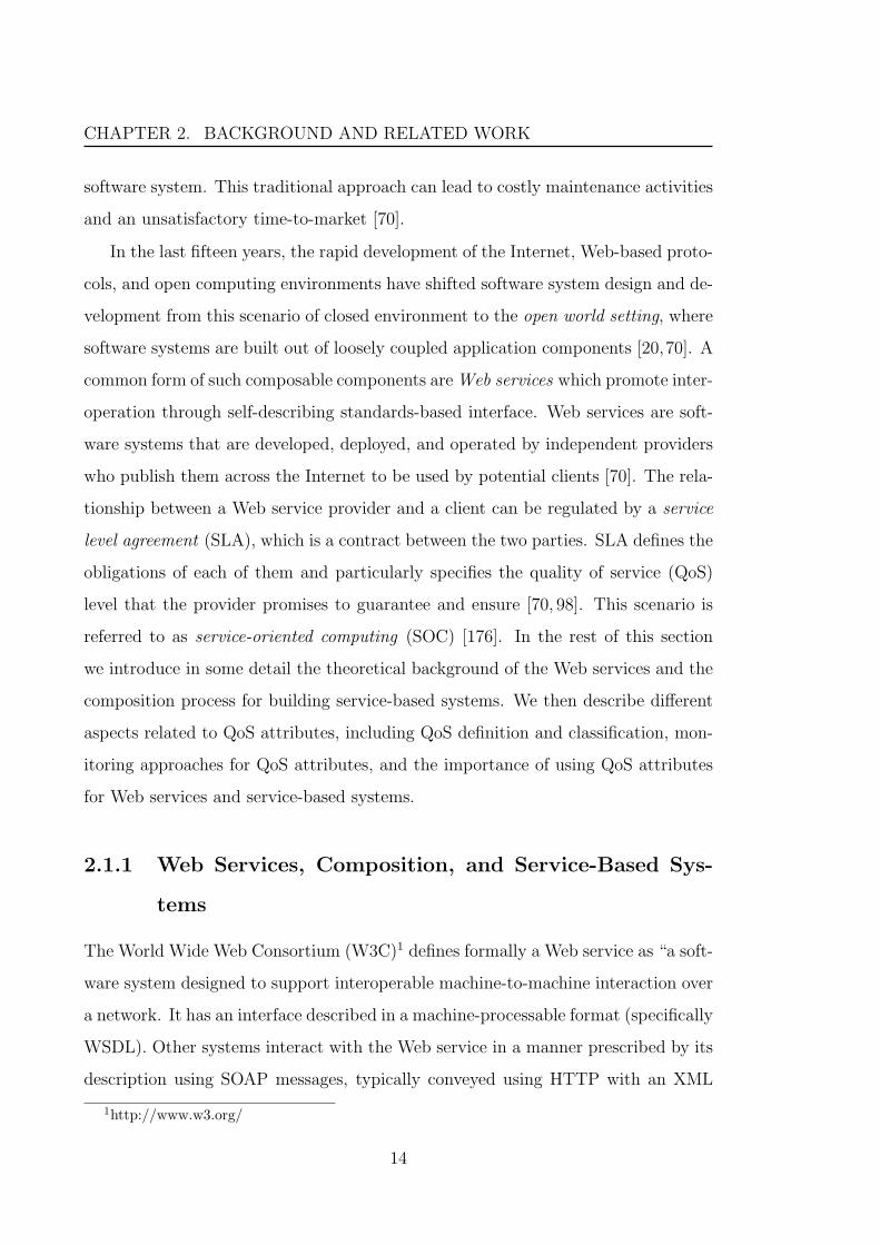
2.1.1 Web Services, Composition, and Service-Based Sys-
tems
The World Wide Web Consortium (W3C)1 defines formally a Web service as “a soft-
ware system designed to support interoperable machine-to-machine interaction over
a network. It has an interface described in a machine-processable format (specifically
WSDL). Other systems interact with the Web service in a manner prescribed by its
description using SOAP messages, typically conveyed using HTTP with an XML
1http://www.w3.org/
14
2.1. BACKGROUND
serialization in conjunction with other Web-related standards” [240]. Web services
are encapsulated, loosely coupled contracted software applications that can be pub-
lished, located, and invoked across the Internet using a set of XML-based standards
such as the SOAP [239] for messaging-based communication, the WSDL [241] for
Web service interface descriptions, and the UDDI [170] for Web service registries.
Thus, Web services can be characterized by three features that are “encapsulated”,
which means their implementation are never seen from the outside, “loosely cou-
pled”, which means changing their implementation does not require change of the
invoking function, and “contracted”, which means there are publicly available de-
scriptions of their behavior, how to bind to them as well as their input and output
parameters [82]. Illustrative examples include Web services that get stock price
information, obtain weather reports, and make flight reservations.
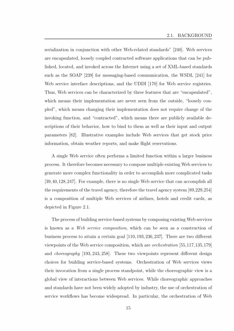
A single Web service often performs a limited function within a larger business
process. It therefore becomes necessary to compose multiple existing Web services to
generate more complex functionality in order to accomplish more complicated tasks
[39,40,128,247]. For example, there is no single Web service that can accomplish all
the requirements of the travel agency, therefore the travel agency system [89,229,254]
is a composition of multiple Web services of airlines, hotels and credit cards, as
depicted in Figure 2.1.
The process of building service-based systems by composing existing Web services
is known as a Web service composition, which can be seen as a construction of
business process to attain a certain goal [110,193,236,237]. There are two different
viewpoints of the Web service composition, which are orchestration [55,117,135,179]
and choreography [193, 243, 258]. These two viewpoints represent different design
choices for building service-based systems. Orchestration of Web services views
their invocation from a single process standpoint, while the choreographic view is a
global view of interactions between Web services. While choreographic approaches
and standards have not been widely adopted by industry, the use of orchestration of
service workflows has become widespread. In particular, the orchestration of Web
15

CHAPTER 2. BACKGROUND AND RELATED WORK
User
Hotel Web Services
Credit Card Web
Services
Airline Web Services
User
Travel Agency
Travel Agency
Figure 2.1: Examples of travel agency systems
services describes the sequence of Web services according to a predefined schema and
run through “orchestration scripts”, which are represented by business processes
that can interact with both internal and external Web services [135, 179]. The
orchestration always represents control from the perspective of one of the business
parties, and the interactions between Web services occur at the message level in
terms of message exchanges and execution order [55,179]. WS-BPEL (Web Service
Business Process Execution Language) [117, 169] is the well-established standard
orchestration language that provides an XML-based grammar for describing the
control logic required to coordinate Web services participating in a composition
process [179,193].
2.1.2 Quality of Service Attributes
A Web service is built to offer a specified functionality that is transparently called
by a software application on another server via Internet-based protocols. The inter-
national quality standard ISO 9126 defines the term functionality as “the capability
16

2.1. BACKGROUND
of the software product to provide functions which meet stated and implied needs
when the software is used under specified conditions” [106]. On the other hand, Web
services are characterized and distinguished by other aspects such as performance,
reliability or safety, which are called non-functional requirements or quality of service
(QoS) attributes. Currently, many QoS attributes are introduced and considered in
the literature. These play an important role in creating, publishing, selecting, and
composing Web services. These QoS attributes are measured in terms of some met-
rics, for example performance can be measured in terms of response time. As a
consequence, because the WSDL can describe only the functional specification of
Web services, other standards such as WS-Policy [31], WSLA [112, 133], and WS-
Agreement [54] have been introduced in order to describe the QoS attributes of Web
services. In addition, some monitoring approaches have been proposed for collecting
QoS data in order to enable the calculation of QoS metrics. In order to introduce
a brief overview for these aspects of QoS attributes, in the rest of this section, a
definition and classification of QoS attributes are introduced along with a listing
of the important QoS attributes. Then, the monitoring approaches for collecting
QoS data are summarized. Finally, the importance of using QoS attributes in Web
services and service-based systems is discussed.
2.1.2.1 QoS Attributes Definition and Classification
Kritikos and Plexousakis [114] define the QoS attributes of Web services as “a set
of nonfunctional attributes of the entities used in the path from the Web service to
the client that bear on the Web service’s ability to satisfy stated or implied needs
in an end-to-end fashion”.
The QoS attributes of Web services can be classified from different perspectives
such as perspectives of domain, measurement, and how QoS values are obtained
[98, 112, 249]. In particular, from the perspective of how QoS values are obtained,
QoS attributes are classified as [98]:
• Provider-advertised attributes: Those attributes that are provided by the Web
17

CHAPTER 2. BACKGROUND AND RELATED WORK
services providers, which are therefore subjective to a providers’ estimation
such as “price or cost” of the Web service.
• Consumer-rated attributes: Those attributes that are computed based on the
Web services consumers’ feedback and evaluation such as “reputation” of the
Web service.
• Observable attributes: Those attributes that are observed and computed based
on monitoring operational events of the Web service. Indeed, majority of the
QoS attributes are measured using observable metrics such as performance,
reliability, availability, and safety [249]. An important characteristic of the
observable QoS attributes is that they are stochastic in nature, and therefore
they might be interpreted in a probabilistic sense using probability distribu-
tions rather than strictly deterministic values [253]. This is because the nature
of those QoS attributes depends on unavoidable and imprecise factors of the
Web services and their context [145,192].
Researchers have introduced and discussed many QoS attributes as important
aspects to the Web services [114, 141, 187, 222, 242]. These QoS attributes include
performance, reliability, availability, accessibility, safety, integrity, and security. In
the following, the observable QoS attributes related to the current research work are
summarized with a discussion of their metrics:
• Performance: The QoS attribute that characterizes how well a Web service
performs, which can be measured in terms of many metrics such as response
time, throughput, latency, execution time, and transaction time [114, 187].
Response time is a required time to complete a Web service request, while
throughput is a number of completed Web service requests at a given time
period. Latency is a round-trip delay between sending a request and receiving
a response, and execution time is a time taken by a Web service to process
its sequence of activities [242]. Finally, transaction time is a required time
for a Web service to complete one transaction, which obviously depends on
18

2.1. BACKGROUND
the definition of Web service transaction. Accordingly, the sum of latency
and execution time gives the response time. In general, faster response time,
higher throughput, lower latency, lower execution time, and faster transaction
time represent good performance of a Web service [242].
• Reliability : Web services should be provided with high reliability which is the
QoS attribute that represents the ability of a Web service to perform its re-
quired functions under stated conditions for a specified time period [114,242].
Indeed, the reliability is the overall measure of a Web service to maintain its
quality, and it is related to the number of failures per day, week, month, or
year [242]. In another sense, reliability is related to the assured and ordered
delivery of messages being sent and received by Web service requesters and
providers [114, 222, 242]. It is usually measured by mean time between fail-
ures (MTBF) metric or the probability that a Web service request has been
correctly responded with a valid response within a specified time period [116].
• Availability : Measures whether a Web service is present or ready for immediate
consumption. Availability represents the probability that a Web service is
available (i.e. up and running) [187, 194, 248]. Larger values indicate that
the Web service is almost always ready to use, while smaller values indicate
unpredictability as to whether the Web service will be available when it is
invoked at a particular time [141]. The availability can be measured as [88,114]:
Availability =< upTime >
< totalT ime >=
< upTime >
(< upTime > + < downTime >), (2.1)
where < upTime > is the total time that a Web service has been up during the
measurement period, while < downTime > is the total time that a Web service
has been down during the measurement period. < totalT ime > is the sum of
< upTime > and < upTime >, which represents the total measurement time.
It is worth mentioning that time-to-repair (TTR), which represents the time
it takes to repair a Web service that has failed, is associated with availability
19

CHAPTER 2. BACKGROUND AND RELATED WORK
[222, 242]. This implies that availability is related to the reliability attribute
[21,191,246]. Kritikos and Plexousakis [114] introduce a new attribute related
to availability which is called continuous availability. Continuous availability
represents the probability that a client can access a Web service an infinite
number of times during a particular time period [114]. Indeed, continuous
availability is different from availability in that it requires subsequent use of a
Web service to succeed for a limited time period [114].
• Accessibility : Characterizes the case where a Web service is available but not
accessible to some users due to external problems such as high volume of
requests or network connection problems [114, 130]. Thus, accessibility is the
quality aspect that represents the degree that a Web service is capable of
serving a client’s requests [222,242]; and it may be expressed as a probability
measure denoting the success rate or the chance of a successful Web service
instantiation at a point in time [141]. Accordingly, Artaiam and Senivongse
[14] propose a metric for measuring accessibility as follows:
Accessibility =< totalRequests >
< totalT ime >, (2.2)
where < totalRequests > is the total number of requests for which a Web ser-
vice has successfully delivered valid responses within an expected time frame,
and < totalT ime > is the total measurement time. Researchers [141,222,242]
point out that high accessibility of Web services can be achieved by building
highly scalable systems, where scalability refers to the ability to consistently
serve the requests despite variations in the volume of requests [141]. It is worth
noting that either non-accessibility or non-availability constitute a “failure”
from the client’s point of view.
20

2.1. BACKGROUND
2.1.2.2 Monitoring Approaches for QoS Attributes
Once a set of QoS attributes has been defined and established for the Web service,
a monitoring approach can be applied to observe the Web service during its current
execution with the aim of collecting detailed data to compute the predefined QoS
metrics. Many monitoring approaches have been proposed in the literature (e.g.
[155,168,187,194]). These monitoring approaches might be:
• Passive or active monitoring: Passive or execution monitoring is a real time
approach that observes a Web service while it passes [187, 208]. On the other
hand, active monitoring is performed when it is required to simulate the Web
service requesters behavior [219]. Mostly, active monitoring is associated with
the online testing of the Web service [147]. Researchers [5,80,177] discuss that
passive and active monitoring approaches are complementary to each other
and they can be used in conjunction with one another.
• Continuous or adaptive monitoring: A Web service might be monitored con-
tinuously or intermittently depending on its application and QoS require-
ments [80]. Thus, continuous monitoring is continually collecting and pro-
cessing data about Web service’s runtime behavior and usage; while adap-
tive monitoring observes a few selected features, and in the case of finding
an anomaly it aims at collecting more data [198]. Actually, the decision of
continuous or adaptive monitoring requires a trade-off between the cost and
overhead of the monitoring and the timely detection of QoS violations [66,168].
• Internal or external monitoring: Monitoring might be performed by Web ser-
vice providers (i.e. internal or server-side monitoring [155]) or by Web ser-
vice requesters (i.e. external or client-side monitoring [194]). Researchers
[153, 235, 253] report that server-side monitoring is usually accurate but re-
quires access to the actual Web service implementation which is not always
possible in practice. On the other hand, client-side monitoring is independent
of the Web service implementation. However, the measured values are affected
21

CHAPTER 2. BACKGROUND AND RELATED WORK
by uncontrolled factors such as networking performance, and they might not
always be up-to-date since client-side monitoring is usually achieved by sending
probe requests [153]. This is why some researchers [80,153] propose combining
the advantages of both server-side and client-side approaches.
2.1.2.3 Importance of Using QoS Attributes in Web Services
QoS attributes play a significant role in the activities of the Web service life cycle. In
the very beginning of these activities, QoS attributes allow the Web service providers
to design the Web service more efficiently according to predefined QoS metrics.
Therefore, the providers know the QoS level that the Web service will exhibit before
making it available to its customers [114]. In addition, the Web service is constructed
in such a way that it is able to provide the required functionalities and fulfil the
QoS requirements. Moreover, in the testing activity, the Web service is checked to
see whether it meets its QoS requirements in addition to functionalities.
QoS attributes are an important factor in the selection of Web services [11]. Par-
ticularly, if there are functionally equivalent Web services available, the customers
can select the Web services based on their functionality as well as their QoS level.
Consequently, there are many QoS-based selection approaches (e.g. [10,11,12,13,29])
introduced in literature that propose using QoS requirements to support selecting
the best Web service that fulfils customer expectations.
QoS attributes can assist in managing the relationship between the Web service
providers and clients. Once the clients select the Web service that they intend to use,
the SLA is constructed as a contract between the clients and providers. Numerical
target values of the QoS attributes, i.e. QoS requirements, play an important role
in this SLA since they are formulated as a collection of service level objectives
(SLOs) [14]. Therefore, for the Web service providers it is important to fulfil these
SLOs and minimize SLA violations in order to avoid paying costly penalties or
breaking the SLA contract [9, 186,217]
QoS attributes of individual Web services are one of the main factors that has
22

2.1. BACKGROUND
to be taken into account in a Web service composition in order to meet the end-
to-end QoS requirements of the constructed service-based systems [248]. In order
to achieve the Web service composition along with optimizing the end-to-end QoS
level, many QoS-aware Web service composition approaches have been proposed
(e.g. [26, 41, 44, 45, 64]). Indeed, these approaches determine the end-to-end QoS of
a composition by aggregating the QoS of the individual Web services and verifying
whether they satisfy the QoS requirements for the whole composition [107, 108].
Therefore, these approaches leverage the structure of a composition that maximizes
the end-to-end QoS level and fulfils the QoS constraints and preferences [248].
Finally, QoS attributes assist in managing the service-based systems. In practical
applications, service-based systems are realized by composing multiple Web services
which are under the control of third-parties, and thus they operate in highly dynamic
and distributed contexts. Therefore, they need to be able to adapt in response to
changes in their context or their constituent Web services, as well as to compen-
sate for violations in QoS requirements [7, 43, 97, 195]. The research community
has developed some approaches to achieve such adaptation which mainly depend on
using QoS attributes (e.g. [50, 144, 153, 156, 224]). In particular, these adaptation
approaches rely on the MAPE-K (Monitor, Analyze, Plan, Execute -Knowledge)
autonomic control loop, which is a general conceptual framework for runtime man-
agement [104].
As depicted in Figure 2.2, the MAPE-K framework consists of four components
- monitoring, analysis, planning, and execution of actions - which are responsible for
maintaining the service-based system functionality as well as the QoS requirements
based on adaptation capabilities. The monitoring component monitors the service-
based system status and collects monitoring QoS data from different Web services.
The monitoring component can achieve this activity by exploiting various proposed
monitoring approaches which are discussed above in the previous subsection. The
analysis component analyzes the monitored QoS data along with the goals stated
in terms of QoS requirements and SLA contacts, and checks for violations of these
23

CHAPTER 2. BACKGROUND AND RELATED WORK
requirements and contracts. Whenever a QoS requirement is violated, the planning
component uses a strategy to create an adaptation plan as a sequence of actions.
Finally, the execution component enforces the planned actions to bring the system
back to the acceptable state.
Autonomic Element
Autonomic Manager
Analyze Plan
Monitor ExecuteKnowledge
Sensors Effectors
Managed Element
Figure 2.2: MAPE-K (Monitor, Analyze, Plan, Execute -Knowledge) autonomiccontrol loop (Cf. [104])
2.2 Review of Related Work
Several approaches have been proposed for detecting violations of QoS requirements
as a critical capability for the management of Web services or service based systems.
As depicted in Figure 2.3, these approaches can be classified into two types; reactive
approaches and proactive approaches. The reactive approaches detect QoS violations
that have already occurred. These approaches can be classified into two groups:
threshold based approaches and statistical based approaches. On the other hand,
the proactive approaches are proposed to proactively detect potential QoS violations
before occurring. They can be classified into three groups: online testing based
approaches, machine learning based approaches, and time series modeling based
24

2.2. REVIEW OF RELATED WORK
approaches.
This section begins with a review of the existing reactive approaches for de-
tecting QoS violations and discusses their limitations. It then reviews the existing
approaches for proactive detection of QoS violations and analyzes their limitations.
Approaches for Detecting QoS Violations
Reactive Approaches Proactive Approaches
Online Testing
Based Approaches
Threshold Based
Approaches
Statistical Methods
Based Approaches
Machine Learning
Based Approaches
Time Series Modeling
Based Approaches
Figure 2.3: Classification of the existing approaches for detecting QoS violations
2.2.1 Existing Approaches for Reactive Detection of QoS
Violations
There are many existing approaches for reactive detection of QoS violations that
are proposed in different application domains, including SLA management, adap-
tations of Web services or service-based systems, and runtime verification of QoS
attributes. These approaches can be classified into two categories: (1) Threshold
based approaches, and (2) Statistical methods based approaches. In the following,
these approaches are reviewed and their limitations are discussed.
2.2.1.1 Threshold Based Approaches
Several approaches have been proposed to monitor QoS attributes at runtime with
the goal of detecting QoS violations in order to trigger adaptations, or to verify
25

CHAPTER 2. BACKGROUND AND RELATED WORK
whether QoS values meet the desired level to detect violations of SLOs. These
approaches detect violations of QoS requirements by observing the running system
and computing QoS values. If these computed QoS values exceed a predefined
threshold, they are considered to be QoS violations.
Siljee et al. [30,215] propose a Dynamic Service Oriented Architecture (DySOA)
which extends service-based systems to make them self-adaptive in order to main-
tain their functionality and ensure they meet their QoS requirements. The general
activity diagram of the DySOA monitoring and adaptation process is depicted in
Figure 2.4. This architecture first uses monitoring to track and collect informa-
tion regarding a set of predefined QoS parameters (e.g. response time and failure
rates), infrastructure characteristics (e.g. processor load and network bandwidth),
and even a context (e.g. user GPS coordinates). The collected QoS information is
analyzed and compared to the QoS requirements that are formalized in the SLA, e.g.
the measured response time is simply compared to the required maximum response
time. If the result of the QoS evaluation indicates that the QoS requirements are
fulfilled, then monitoring continues. If one of the the QoS requirements is violated,
a new configuration might be chosen that will satisfy the QoS requirements. Finally,
the changes are enacted in the system. Possible changes are substituting a bound
Web service for an alternative Web service or changing the structure and the flow
of the Web service composition.
In [131,132], a middleware architecture is proposed to enable SLA-driven cluster-
ing of QoS-aware application servers in order to guarantee the QoS requirements and
meet the SLAs of hosted Web services and applications. This middleware consists of
three components which work as services, as depicted in Figure 2.5. The monitoring
service observes at runtime the Web services and applications and verifies whether
the QoS values meet the desired level to detect violations of SLAs, the load balanc-
ing service intercepts client requests to balance them among different cluster nodes,
and the configuration service is responsible for managing the QoS-aware cluster.
If the QoS values delivered by the cluster deviate from the desired level (e.g. the
26

2.2. REVIEW OF RELATED WORK
Collect monitoring data Determine QoS Evaluate QoS
[Qos is ok]
Determine new configurationEnact change in system
[Qos is not ok]
Figure 2.4: General activity diagram of the DySOA monitoring and adaptationprocess (Cf. [215])
response time breaches the predefined threshold), the middleware reconfigures that
cluster by adding clustered nodes.
Requests
Responses
ClienttsLoad
Balancing
Service
ClusterConfiguration
Service
Monitoring
Service
Desired QoS
Hosting SLA
Figure 2.5: QoS-aware middleware services interaction (Cf. [132])
In his Master’s thesis, Hilari [98] developed an architecture, which built on the
SALMon1 project [5], for monitoring the QoS information of a Web service and
detecting SLA violations. This architecture consists of three services: Monitor,
Analyzer, and Decision Maker. While the Monitor service collects the information
about QoS attributes, the Analyzer service is responsible for checking any SLA
1http://appserv.lsi.upc.es/salmon/
27
CHAPTER 2. BACKGROUND AND RELATED WORK
violations in service-based systems. When a violation is detected, it is notified to
the Decision Maker service of the affected system.
Michlmayr et al. [153] have presented an event-based QoS monitoring and SLA
violation detection framework. This framework combines the advantages of client-
side and server-side QoS monitoring, and it is integrated in the VRESCo1 [152,154],
which is a run-time environment for service-oriented computing. The framework
observes the QoS values and checks whether they meet the required levels to detect
possible violations of SLAs. Once an SLA violation is detected, notifications are
sent to interested subscribers using E-Mail or Web service notification.
Recent studies [156, 224] propose autonomic frameworks to monitor QoS at-
tributes and dynamically adapt service-based systems in an automated manner in
response to QoS requirement violations. In [156], Mirandola and Potena propose
a framework that dynamically adapts a service-based system while minimizing the
adaptation costs and guaranteeing a required level of QoS. This framework triggers
adaptation actions automatically in response to runtime violation of system QoS
constraints, or the availability/non-availability of Web services in the environment.
Thongtra and Aagesen [224] present a framework for Web service configuration that
has goals, which express required performance and income measures, and policies,
which define actions in states with unwanted performance and income measures.
This framework monitors QoS attributes constraints and in the case of violations it
triggers pre-defined policies.
2.2.1.2 Statistical Methods Based Approaches
A number of approaches have been proposed based on statistical methods in order to
detect QoS violations. In contrast to threshold based approaches, these approaches
observe the computed QoS values at runtime and use statistical methods in order to
detect timely QoS violations with statistical confidence. In general, the statistical
methods used by these approaches include relative frequency, hypothesis testing,
1Vienna Runtime Environment for Service-oriented Computing
28
2.2. REVIEW OF RELATED WORK
and sequential probability ratio test [159,232].
Mosincat et al. [161, 162] propose an approach, called ADULA, for transpar-
ent runtime monitoring, automated performance degradation detection, diagnosis,
and repair for Web service compositions, which are expressed as BPEL (Business
Process Execution Language) processes. The ADULA approach checks the fulfill-
ment of SLA guarantees and determines if a violation has occurred using statistical
hypothesis testing [159], implemented by a component called violation detectors.
When a violation of SLA guarantees is detected, the approach diagnoses the cause
of the violation and dictates repair actions, which include Web service replacement
in subsequent process instances.
Authors in [8, 180, 181] propose an approach for the evolution and adaptation
of Web services in order to provide the agreed QoS requirements stated in the
SLA contract. This approach provides a compatibility mechanism that measures
the aggregated satisfaction value of offered Web services to verify whether the QoS
changes are satisfiable according to the existing contract. The approach uses fuzzy
parameters to understand to what extent the QoS parameters are violated/satisfied
and to compute the satisfaction function. Then, the degree of satisfaction function is
evaluated. The existing contract will remain valid between the Web service provider
and customer as long as the satisfaction value is more than the nominated in the
contract. If the satisfaction value is less than the agreed value, the contract is
voided and an adaptation/evolution strategy needs to be proposed such as Web
service replacement.
Authors in [196] discuss some resource metrics for distributed systems that con-
form to the service-oriented concepts and cover various quality aspects. A QoS
requirements satisfaction is analyzed by assessing the degree of SLA fulfilment or
SLA violation danger. This degree is classified to a few distinct states. If the SLA
is characterized as green, then all SLA conditions are fulfilled; yellow then SLA con-
ditions are met but indicators come near to the predefined thresholds; or red then
SLA conditions are not satisfied. Based on this classification of SLA status, the SLA
29
CHAPTER 2. BACKGROUND AND RELATED WORK
violation danger is measured as a ratio of the time for a Web service operation with
yellow SLA to the time with yellow and green SLA.
Rosario et al. [25, 192] argue that QoS requirements are typically stated in the
form of hard guarantees in SLA (e.g. response time always less than 2 seconds),
however, experiments and measurements from existing Web services show evidence
that soft guarantees, not hard, should be stated instead (e.g. response time less
than 2 seconds in 95% of the cases). Therefore, they present the notion of soft
probabilistic requirements (or contracts), especially for the performance attribute, in
order to enable flexibility in SLA compliance. With this approach, QoS requirements
are characterized by means of a set of selected quantiles of probability distributions
for the QoS attributes. Moreover, they propose an approach to detect violations
of the agreed SLA based on the statistical testing that depends on the empirical
distribution function of the QoS attributes.
The work in [23, 24] proposes a generic application-independent framework for
monitoring and analyzing QoS attributes of the Web services. The proposed frame-
work has been adopted in the European WS-DIAMOND1 project for providing self-
healing solutions for service-based systems [24]. This framework provides models
to detect QoS violations. These models use descriptive statistics, e.g. averages
and standard deviations, to compute the QoS threshold as “average + standard
deviation”. Also, they use temporal patterns to avoid considering transient QoS
violations. For instance, if there are only one or two values above the QoS thresh-
old, they may not be classed as a violation; but if there are three successive values
above the threshold, they are classified as such. Hence, this framework computes the
thresholds at runtime to monitor the evolution of the given QoS characteristics more
than their absolute values. It is worth noting that this approach proposes comput-
ing the threshold based on the descriptive statistics without statistical confidence,
and there are not concrete rules for the proposed temporal patterns. However, this
approach can be improved by using statistical methods, especially Shewhart control
1Web Services - DIAgnosability Monitoring and Diagnosis
30

2.2. REVIEW OF RELATED WORK
charts methodology with Supplementary Runs Rules [157].
Schulz [206] proposes a metric, which is a linear function of given QoS thresh-
olds, to quantify the degree of SLA fulfillment. This metric takes into account the
underlying structure of the SLA as well as the available options for monitoring QoS
attributes. Using this metric, it becomes possible at runtime to obtain detailed in-
formation of the status of a Web service compliance. This approach gives a percent
of satisfying QoS requirements, which might speed the detection of QoS violations
by continuously monitoring the satisfaction level.
Chan et al. [48] propose an approach that provides a rich platform in .NET appli-
cations for monitoring QoS requirements by checking constraints written in PCTL
(Probabilistic Computation Tree Logic) [94]. Its methodology is simply calculating
the relative frequencies of successful and unsuccessful monitoring results, and then
comparing them with the required probability. Based on these calculated relative
frequencies and the required probability, it decides whether the QoS requirements
are satisfied. It is worth mentioning that, this approach can be further improved
by using the sequential hypothesis testing as a good method to make statistically
significant decisions [232].
Sammapun et al. [200, 201] propose an approach, which is called MaC, adopts
statistical hypothesis testing for verifying QoS requirements defined in a probabilistic
extension of the Meta-Event Definition Language (MEDL). The main idea of this
approach is to sample many execution paths, estimate the probability of success,
and then apply hypothesis testing method to check for probabilistic property and
make statistically significant decision regarding this property with a given confidence
level. Using this methodology, it is able to investigate properties with a single
probabilistic operator and provide p-value for the significance of the testing outcome-
based-decision. To overcome false alarms problem resulted from considering too
many samples, it uses the sliding window that keeps the number of samples used in
monitoring constant and pre-defined.
Grunske and Zhang [87] propose a monitoring framework called ProMo (Prob-
31

CHAPTER 2. BACKGROUND AND RELATED WORK
abilistic Monitoring). This framework adopts a probabilistic temporal logic called
CSLMon, which is a subset of the continuous stochastic logic (CSL) [15, 17], to de-
fine probabilistic properties. It samples execution paths and checks whether the
probabilistic properties are satisfied using acceptance sampling and sequential prob-
ability ratio test (SPRT) [232] with given confidence and power levels. Sequential
hypothesis testing is considered the most effective testing procedure with respect to
the number of execution paths needed to apply the test and check the correctness
of probabilistic properties [244]. Therefore, this approach has some relative advan-
tages over the other statistical methods based approaches. Further improvement for
this approach has been proposed by Grunske [86] to support continuous monitoring
and minimize the number of required samples and the runtime overhead to reach a
decision.
2.2.1.3 Summary and Limitations of Reactive Approaches
The reactive approaches reviewed above are summarized in Table 2.1. Based on the
summary, some observations can be highlighted:
• Web services : Most of the reviewed reactive approaches are applied to com-
posite Web services (or service-based systems), and only three approaches are
applied to individual Web services. It is worth mentioning that the approaches
proposed by Chan et al. [48], Sammapun et al. [200, 201], and Grunske and
Zhang [86, 87] for runtime verification of QoS attributes are applied generally
to software systems and not specifically to Web services. However, the work
of Grunske and Zhang [86, 87] has been already integrated into the QoSMOS
(QoS Management and Optimization of Service-based systems) framework [37]
that is proposed for the development of adaptive service-based systems.
• QoS attributes : Performance, reliability, and availability are the main three
QoS attributes that are considered by the reviewed approaches, respectively.
In addition, some approaches claim that other QoS attributes can be added
32

2.2. REVIEW OF RELATED WORK
and considered by the proposed approaches.
• Application domain: The application domains of the reviewed reactive ap-
proaches are mainly three: (1) SLA management, (2) Adaptation of Web ser-
vices or service-based systems, and (3) Runtime verification of QoS attributes.
However, the adaptation domain is the most targeted by the proposed ap-
proaches.
• MAPE-K autonomic control loop: The summary in Table 2.1 shows that the
reviewed approaches implement some or all of the activities of the MAPE-K
autonomic control loop. In general, all the approaches implement the “Ana-
lyze” activity, and most of the approaches proposed in the adaptation domain
implement the four activities of the MAPE-K loop.
• How QoS data is obtained : Most of the reviewed approaches use the QoS data
that is collected from the provider-side. Other approaches use the QoS data
that is collected from the client-side, both client-side and provider-side, or not
specified.
• Probability distribution: As mentioned above, the statistical methods based ap-
proaches report that the observable QoS attributes are probabilistic in nature,
and therefore they can be represented by a probability distribution. However,
the summary shows that few approaches evaluate or consider the probability
distribution of the QoS attributes.
• Serial dependency : Since the QoS data is collected over time, it is expected
to be serially dependent. However, the reviewed statistical methods based ap-
proaches use the statistical methods such as hypothesis testing and sequential
probability ratio test that assume the data is independent without evaluating
this assumption. Note that Grunske and Zhang [87] acknowledge this limita-
tion and mention that they will address in their future work.
33

CHAPTER 2. BACKGROUND AND RELATED WORK
Threshold Based Statistical Methods Based
Silje
eet
al.
[30,
215]
Lodi
etal
.[1
31,1
32]
Hilar
i[9
8]
Mic
hlm
ayr
etal
.[1
53]
Mir
andol
aan
dP
oten
a[1
56]
Thon
gtra
and
Aag
esen
[224
]
Mos
inca
tet
al.
[161
,162
]
Per
nic
iet
al.
[8,1
80,1
81]
Rud
etal
.[1
96]
Ros
ario
etal
.[2
5,19
2]
Hal
ima
etal
.[2
3,24
]
Sch
ulz
[206
]
Chan
etal
.[4
8]
Sam
map
un
etal
.[2
00,2
01]
Gru
nsk
ean
dZ
han
g[8
6,87
]
1. Web Service C C C I C C C C I C C I N N N
2. QoS
Performance X X X X × X X X X X X X X ∼ ∼Reliability × × × × X × X X X × × × ∼ X X
Availability X X X X × × × × × × × X ∼ ∼ ∼3. Application A A A S A A A A S S A S V V V
4. MAPE-K
Monitor X X X X X X X × × X X × × × ×Analyze X X X X X X X X X X X X X X X
Plan X X X × X X X X × × × × × × ×Execute X X X × X X X X × × × × × × ×
5. Data Cl Pr Pr CP Pr Pr Cl N Pr Pr CP N Pr Pr Pr
6. Distribution × × × X × × × X X
7. Dependency × × × × × × × × ∼(C) Composite, (I) Individual, (N) Not specified, (X) Supported, (×) Not supp-
orted, (∼) Can be supported, (A) adaptation, (S) SLA management, (V) Run-
time Verification, (Cl) Client side, (Pr) Provider side, (CP) Client side and Pro-
vider side.
Table 2.1: Summary of reactive approaches
In general, the reactive approaches detect violations of QoS requirements after
they have occurred. Therefore, this reactive detection of violations leads to critical
issues. For example, SLA management cannot avoid costly compensation and repair
activities resulting from violating SLA contracts. In addition, adaptation is triggered
34
2.2. REVIEW OF RELATED WORK
after violations and problems have already occurred. In particular, such reactive
adaptations have several important drawbacks that are discussed in literature [97,
111,149,204]. These drawbacks can be summarized in the following:
1. Reactive adaptations might come too late to the extent that faulty Web ser-
vice or service-based system are executed, which can lead to undesirable con-
sequences such as loss of money or transactions and unsatisfied users as well
as might require the execution of additional activities such as compensation
or roll-back [111,149].
2. In an emergency situation such a reactive adaptation can lead to critical situ-
ations. For example, it might delay the timely dispatch of operational forces,
e.g. fire engines or ambulances [204].
3. In some cases the reactive detection of violations is very late to the extent that
an adaptation of the system is not possible anymore, because the system has
already terminated in an inconsistent state [97].
4. In some cases executing adaptation activities reactively can considerably in-
crease execution time compared to executing activities before violations occur,
and therefore might reduce the overall performance of the running Web service
or service-based system [97].
2.2.2 Existing Approaches for Proactive Detection of QoS
Violations
In order to address the limitations of the existing reactive approaches, some ap-
proaches have been proposed for the proactive detection of potential QoS violations.
Generally, the proactive approaches aim to prevent SLA violations and support
proactive adaptation. Preventing SLA violation refers to that the SLA management
predicts a menacing SLA violation and proactively performs preventive actions in
order to avert the violation before it occurs [204]. On the other hand, proactive
35

CHAPTER 2. BACKGROUND AND RELATED WORK
adaptation means the Web service or service-based system will detect the need for
adaptation and will self-adapt before a violation of QoS requirements will occur or
lead to undesired consequences [178].
As mentioned above, the proposed approaches for proactive detection of potential
QoS violations can be classified into three main groups: (1) Online testing based
approaches, (2) Machine learning based approaches, and (3) Time series modeling
based approaches. In the following, these approaches are summarised with some
details about their underlying methodology, advantages, and shortcomings.
Online Testing Based Approaches
Online testing based approaches [65,97,149,150,202] exploit online testing techniques
to detect QoS violations before they occur in order to proactively trigger adaptation
requests. Online testing means that the Web service or service-based system is tested
(i.e. fed with dedicated test input) in parallel to its normal use and operation [147].
The main idea behind using the online testing is that an online test can detect a
violation if a faulty Web service instance is invoked during the test. This points
to a potential problem that the service-based system might face in the future of its
operation when invoking this faulty Web service instance. In such a case, adaptation
activities can be proactively triggered to prevent the potential violation. These
adaptation activities might include replacing the faulty Web service instance with
another instance or changing the Web service composition.
The online testing based approaches rely on three assumptions, which are [149]:
• Assumption 1: Each failure of a constituent Web service of a service-based
system leads to a requirement violation of that service-based system and thus
the need for an adaptation arises.
• Assumption 2: The observed elements provide a notification in case of any
change which would invalidate the testing data, such as a new version of the
Web service implementation.
36

2.2. REVIEW OF RELATED WORK
• Assumption 3: Invoking the constituent Web services of a service-based system
for test purposes will have no side effects, such as when testing a book delivery
Web service, no books would actually be delivered as a result of the testing
activities.
Metzger et al. discussed that the online testing assumptions can be relaxed
and mitigated as presented in their work [149]. However, they are still hard to
be typically fulfilled and hold for the real application of service-based systems. In
addition to these assumptions, there are some shortcomings related to online testing
that might limit the practical applicability of these approaches. These shortcomings
are:
• Providing only general statements : Online testing can provide only general
statements about Web services or service-based systems but not about their
current execution traces as can be achieved by monitoring approaches [27,
163]. This point is already raised in the literature and discussed as one of
the advantages of monitoring approaches over testing [59]. Therefore, some
failures and violations cannot be uncovered and might escape testing because
the concrete input that leads to the current execution trace might not be
covered by any test case [149].
• Requiring additional costs : Online testing applied to service-based systems
might lead to additional costs. This is because the service-based systems often
include external Web services whose invocations are associated with costs [149].
Machine Learning Based Approaches
Machine learning based approaches [118, 119, 120, 121, 122] use techniques from the
areas of machine learning [96] to construct prediction models in order to proactively
detect potential violations of QoS requirements and agreed SLA contracts. These
approaches leverage machine learning capabilities to train prediction models using
previously monitored historical QoS data. For example, collected historical QoS
37

CHAPTER 2. BACKGROUND AND RELATED WORK
data can be fed into multi-layer artificial neural networks [96] as training dataset in
order to generate predictions of the future SLA violations.
The effectiveness of machine learning based approaches relies on the historical
QoS data, which is required as a training dataset, and the training process [204]. For
ensuring the expected accuracy of the SLA violation prediction, several hundreds
or, in some cases, even thousands of QoS data points are necessarily required to
train prediction models. Indeed, this can limit the applicability of these approaches
if only a small amount of historical data is available [204]. Moreover, the prediction
models have to be re-trained after each adaptation of the service-based systems,
which is a time-consuming and computationally intensive process [165].
Time Series Modeling Based Approaches
Several approaches (e.g. [73, 80, 218, 251, 252]) have been proposed based on time
series modeling for proactive detection of potential QoS violations, especially linear
ARIMA (Autoregressive Integrated Moving Average) models [33]. Simply, the key
idea of these models is to fit the past monitored QoS measures in order to forecast
their future values and violations of predefined requirements. Time series models can
be applied for QoS measures starting with 30 historical observations and can give
acceptable forecasting accuracy [33]. The main advantage of the time series modeling
based approaches is that they In addition, they are data-oriented approaches and
do not impose any restrictive assumptions on the environment of the Web service
or service-based system. Moreover, because time series modeling’s methodology is
based on standard statistics theory and probability distributions, prediction models
can be straightforwardly implemented without a time-consuming learning stage as
is the case with machine learning models.
These three groups of approaches can be briefly compared in different dimen-
sions, as depicted in Table 2.2. First, based on the cost in terms of the computa-
tional overhead (and the additional cost associated with the invocations of external
Web services), the online testing based approaches are the most expensive, followed
38

2.2. REVIEW OF RELATED WORK
by the machine learning based approaches. Statistical methods based approaches
are the least expensive. Second, online testing based approaches are environment-
dependent, whereas machine learning based approaches and time series modeling
based approaches are not. The third dimension is timeliness which means how fast
the approach can be used to detect potential violations of QoS requirements. Based
on the timeliness, the online testing based approaches are the best because they do
not require historical QoS data to be applied, followed by the time series modeling
based approaches which require less historical QoS data to construct a forecasting
model compared to the machine learning based approaches.
Enviroment-
Approaches Cost Dependant Timeliness
Online Testing Based (3) Yes (1)
Machine Learning Based (2) No (3)
Time Series Modeling Based (1) No (2)
(i) Rank “i” among the approaches.
Table 2.2: Summary of proactive approaches
Based on this brief comparison, it can be seen that the time series modeling
based approaches are promising in their ability to provide accurate forecasting for
QoS attributes and potential violations of their requirements. Indeed, the accurate
QoS forecasting is essentially required in order to avoid violating SLA constraints,
missing proactive adaptation opportunities, and executing unnecessary proactive
adaptations. In particular, missing a proactive adaptation opportunity due to in-
accurate QoS forecasting can obviously lead to the same shortcomings as faced in
the setting of reactive adaptations, e.g. it can require costly compensation or repair
activities. Eventually, this would diminish the benefits of proactive adaptation [147].
Moreover, unnecessary adaptations can lead to critical shortcomings [147,148,149]:
- First, unnecessary adaptations can be costly even in the proactive setting,
especially when a seemingly unreliable but cheap Web service is replaced by a
more costly one. Moreover, additional activities, such as SLA negotiation for
39

CHAPTER 2. BACKGROUND AND RELATED WORK
the alternative Web services, might have to be achieved [149].
- Second, unnecessary adaptations may lead to instabilities in the software sys-
tem which can lead to unreliable and inconsistent behavior. Therefore, unnec-
essary adaptations should be avoided [149].
Consequently, the goal of this thesis is to propose an efficient time series modeling
based QoS forecasting approach that can accurately forecast QoS attributes and
potential violations of their requirements. Accordingly, in the following we review
the existing time series modeling based approaches and identify the main challenges
that have to be addressed to achieve this goal.
2.2.2.1 Existing Approaches Based on Time Series Modeling
Time series modeling based proactive approaches have been presented as a promis-
ing technique to predict future QoS values in order to support proactive adaptation
of service-based systems, SLA management, failure management, and QoS-based
service selection and composition in dynamic environments. Zeng et al. [250] inves-
tigate performance metrics that can be predicted based on their historical data and
using time series models. Their work introduces the design and implementation of
an event-driven QoS prediction system, which can process operational service events
in a real-time fashion, in order to predict or refine the prediction of performance
metrics. Recently, Solomon and Litoiu [218] present a dynamic predictive model
based on linear regression and ARIMA models to predict with more confidence
system performance degradations. They also propose a feedback based evolution
architecture that can proactively, using these performance degradations predictions,
tune and optimize software systems.
Current studies [72, 73, 147, 252] propose failure prediction techniques to enable
and enhance proactive failure management by avoiding possible failures. In [72,73],
Fu and Xu develop two models: (1) Spherical covariance model with an adjustable
timescale parameter in order to quantify the temporal correlation, and (2) Stochastic
40

2.2. REVIEW OF RELATED WORK
model in order to characterize spatial correlation. Therefore, they become able to
cluster failure events based on their correlations and predict their future occurrences
using time series autoregressive models. In addition, Zhang and Fu [252] propose
a framework for autonomic failure management. They equip the framework with
the failure prediction functionality in order to achieve proactive self-management
of both failures and resources in networked computer systems. This framework
analyzes node, cluster, and system failure behaviors. Then, based on quantified
failure dynamics, it forecasts prospective failure occurrences using linear time series
models, especially autoregressive models.
Recently, Metzger et al. [147, 148] discuss two directions along which accurate
proactive adaptations can be achieved. These two directions are: (1) Improving the
failure prediction techniques that trigger the need for adaptations, and (2) Estimat-
ing the accuracy of the predicted failures at runtime. While Metzger et al. in this
work use only simple prediction models such as the arithmetic average and simple
exponential smoothing, they recommend using the advanced time series prediction
models in future work.
In the context of QoS and SLA management, Nobile et al. [166] propose an
architecture that supports QoS for RT-RPCs (Real-Time Remote Procedure Calls),
which are widely used in the implementation of distributed applications. To enable
proactive management, the architecture uses ARIMA models in order to predict
future traffic characteristics of RT-RPCs that pass through the proxy. Therefore, the
architecture is furnished with the capability of allowing the anticipated and rational
allocation of the necessary resources to attend the predicted demand. In [257], Zhu
et al. present a framework that is designed to help predict the performance of
parallel/distributed discrete event simulation (PDES) applications. In particular,
the framework uses linear time series analysis to forecast the future performance of
PDES in order to proactively evaluate and optimize the QoS of PDES programs.
In the domain of QoS-based Web service selection and composition, Vu et al. [231]
present a QoS-based Web service selection and ranking approach, which uses trust
41

CHAPTER 2. BACKGROUND AND RELATED WORK
and reputation evaluation techniques as well as linear regression models in order
to predict the future QoS of Web services. Based on the predicted QoS values,
the approach selects and ranks the Web services. The output is a list of Web
services which fulfill QoS requirements of a user and are ordered by their prospective
satisfaction levels of the given QoS criteria. Li et al. [123] propose a Web service
selection algorithm based on a QoS prediction mechanism. This algorithm uses time
series modeling based on structural equations to fit QoS values of Web services, and
dynamically predicts their future changes in order to support adaptive Web services
selection. In addition, Godse et al. [80] propose a method that combines monitoring
and extrapolation methodologies based on ARIMA models to predict Web service
performance. This method is used to support automating dynamic service selection
methodology, which is robust in the face of varying QoS.
As an evaluation for the existing QoS forecasting approaches based on time series
modeling, Cavallo et al. [46] present an empirical study aimed at comparing different
approaches for QoS forecasting. Specifically, the approaches being compared are:
(1) The averaged value from past monitored QoS data, (2) The last observed QoS
value which is referred to as “current QoS value”, (3) linear regression model, and
(4) Time series ARIMA model. The study is performed on QoS data obtained by
monitoring the execution of ten real Web services for four months. It concludes that
ARIMA forecasting is the best compromise in ensuring a good prediction error, being
sensible to outliers, and being able to predict likely violations of QoS constraints.
2.2.2.2 Summary and Limitations of Time Series Modeling Based Ap-
proaches
The time series modeling based proactive approaches reviewed above are summarized
in Table 2.3, and some observations can be highlighted in the following:
• Web services : Most of the reviewed approaches are applied to Web services
(especially individual Web services). However, some approaches are applied
generally to software systems and not specifically to Web services.
42

2.2. REVIEW OF RELATED WORK
• QoS attributes : Similarly to reactive approaches, Performance, reliability, and
availability are the main three QoS attributes that are considered by the re-
viewed proactive approaches, respectively.
Zen
get
al.
[250
]
Sol
omon
and
Lit
oiu
[218
]
Fu
and
Xu
[72,
73]
Zhan
gan
dF
u[2
52]
Met
zger
etal
.[1
47,1
48]
Nob
ile
etal
.[1
66]
Zhu
etal
.[2
57]
Vu
etal
.[2
31]
Li
etal
.[1
23]
Godse
etal
.[8
0]
Cav
allo
etal
.[4
6]
1. Web Service X X × × X × × X X X X
2. QoS
Performance X X × × X X X X × X X
Reliability × × X X × × × × X × ×Availability × × × × × × × × X X ×
3. Application S A F F A A A Se Se Se Se
4. MAPE-K
Monitor X X × × × X × × × X ×Analyze X X X X X X X X X X X
Plan × X × × × X × × × × ×Execute × X × × × X × × × × ×
5. Data Cl Pr Pr Pr Cl Pr Pr Cl Pr CP Cl
6. Distribution × × × × × × × X × X ×7. Dependency X X X X X X X X X X X
8. Stationarity × X × × × X × × × X X
9. Nonlinearity × × × × × × × × × × ×(X) Supported, (×) Not supported, (A) adaptation, (S) SLA mana-
gement, (F) Failure management, (Se) Service selection, (Cl) Client
side, (Pr) Provider side, (CP) Client side and Provider side.
Table 2.3: Summary of time series modeling based proactive approaches
• Application domain: The reviewed proactive approaches are proposed in dif-
ferent application domains, which include SLA management, adaptation of
43

CHAPTER 2. BACKGROUND AND RELATED WORK
Web services (or generally software systems), failure management, and service
selection and composition.
• MAPE-K autonomic control loop: The reviewed approaches implement the
“Analyze” activity, and only a few approaches implement other activities of
the MAPE-K loop.
• How QoS data is obtained : The reviewed proactive approaches use the QoS
data that is collected from the provider-side, client-side, or both client-side
and provider-side, respectively.
• Probability distribution: Only two approaches consider the probability distri-
bution of the QoS data.
• Serial dependency : All the reviewed approaches assume the QoS data is serially
dependent, and introduce time series modeling to predict future values.
• Stationarity : Broadly speaking, stationarity means that the mean and the
variance of the data are constant over time and its autocovariance is not time
varying and is only a function of the time distance between the observations
[67, 167]. Stationarity enables the time series model to estimate the mean,
variance, and other parameters by averaging across the single realization of the
data, which explains why the time series models assume the data is stationary
or can be stationarized using transformation methods [33]. However, only few
of the reviewed approaches mention and check the stationarity of the QoS
data.
• Nonlinearity : Time series models are traditionally divided into two classes;
linear and non-linear, and specifying the class that can be used should be
based on evaluating the QoS data. Practically, linear time series models are
easier to use. This may be why none of the reviewed approaches evaluate the
nonlinearity of the QoS data and rather use linear time series models.
44

2.2. REVIEW OF RELATED WORK
In general, authors of the existing time series modeling based approaches con-
clude that time series models are initially a good statistical tool to model the dy-
namic behavior of QoS attributes and forecast their future values. However, Godse
et al. [80] report that studying the dynamic characteristics of QoS attributes and
proposing an efficient QoS forecasting approach is a crucial need in order to support
proactive QoS management and Web service selection. Moreover, Cavallo et al. [46]
conclude based on their empirical study that a good forecasting of QoS violations
is still a challenging issue and further approaches able to better deal with this issue
should be investigated.
Based on our review of these existing proactive approaches, we can summarize
their main limitations as follows:
• Although QoS attributes are mentioned that are probabilistic and have
stochastic characteristics, these stochastic characteristics are not studied
or evaluated based on real QoS data. This evaluation of QoS stochastic
characteristics is very important to select and use an appropriate time series
model that can adequately fit QoS attributes and accurately forecast their
future values.
• Only linear time series models, especially ARIMA models, are used by these
approaches. Moreover, these linear models are mostly used without checking
their underlying assumptions or evaluating their adequacy. This implies that
using time series models without satisfying their assumptions can provide inac-
curate forecasts, which in turn leads system management to take inappropriate
or unnecessary actions based on incorrect information.
• There is no discussion of how those linear time series models can be con-
structed at runtime as well as how they can be continuously updated based
on evaluating their adequacy and forecasting accuracy.
Addressing these limitations is very important to guarantee accurate forecasting
for QoS attributes and potential violations of their requirements. Therefore, the
45

CHAPTER 2. BACKGROUND AND RELATED WORK
goal in this thesis is to propose a forecasting approach for QoS attributes that can
address the above limitations and provide accurate QoS forecasting. In the rest of
this thesis, the main challenges of achieving this goal are formulated into research
questions and then addressed as contributions of the thesis. The outcome of address-
ing these research questions is a collection of QoS characteristic-specific forecasting
approaches based on time series modeling that construct together a general auto-
mated forecasting approach. This general forecasting approach will be able to fit
different dynamic behavior of QoS attributes in order to forecast their future values
and potential violation of their requirements.
2.3 Summary
This chapter first presented the background of the contents presented in the remain-
der of the thesis, starting with a brief introduction to Web services, compositions,
and service-based systems. Then, because the Web services and service-based sys-
tems are characterized by QoS attributes in addition to functionality specifications,
the chapter described different aspects related to QoS attributes, including QoS
definition and classification, monitoring approaches for QoS attributes, and the im-
portance of using QoS attributes for Web services and service-based systems.
The second part of the chapter reviewed the existing approaches for detecting
violations of QoS requirements. These approaches are classified into reactive ap-
proaches that are based on monitoring techniques and proactive approaches that are
based on anticipating potential QoS violations. In particular, it reviewed in detail
the existing time series modeling based proactive approaches and highlighted their
limitations. These limitations represent the challenges that have to be addressed in
this thesis in order to provide accurate QoS forecasting.
46

Chapter 3
Research Methodology
The previous chapter presents the background on Web services, composition, QoS
attributes, and adaptation of service-based systems followed by a review of the exist-
ing reactive and proactive detection approaches for QoS violations and a discussion
of their limitations. These limitations are related to providing accurate forecast-
ing for QoS attributes and potential requirements violations. Accordingly, in order
to address the limitations of the existing approaches, the goal of this research is
“to develop a general automated statistical forecasting approach based on time se-
ries modeling for QoS attributes”. This forecasting approach will automatically fit
the dynamics of QoS attributes in order to accurately forecast their future values
and detect proactively potential future violations of QoS requirements. Achieving
this goal is key prerequisite to support proactive SLA management, proactive ser-
vice selection and composition, and the proactive adaptation of Web services or
service-based systems.
In order to achieve the overall research goal, a number of research questions need
to be addressed. Indeed, explicitly formulating the research questions helps structure
the research activities and highlights the novelty of a solution and the contributions
of the research work [79, 209]. Therefore, the next section formulates the research
questions that have to be addressed in the thesis, followed by an overview of the
research approach that is applied in order to address these formulated research
47

CHAPTER 3. RESEARCH METHODOLOGY
questions. Finally, the strategy used to evaluate the contributions in this thesis is
discussed at the end of the chapter.
3.1 Research Questions
The research goal is planned to be achieved by formulating the limitations of existing
proactive approaches into refined research questions that will be addressed in the
thesis. These research questions are discussed as follows.
RQ1. To what extent do the QoS attributes of real-world Web services exhibit
stochastic characteristics related to time series modeling?
From a statistical standpoint, proposing an efficient and accurate forecasting ap-
proach that fits the QoS attributes and forecasts their future values requires the key
stochastic characteristics of these attributes to be identified and evaluated. This
is because the accuracy of the proposed forecasting approach is statistically based
on the QoS stochastic characteristics. Based on th literature of time series analysis
and modeling (e.g. [33, 103, 158, 184]), we identify a number of key stochastic char-
acteristics that have to be considered in order to guarantee accurate forecasting.
These stochastic characteristics include probability distribution, serial dependency,
stationarity, and nonlinearity. In Chapter 2, we introduced these stochastic char-
acteristics and checked whether the existing approaches studied or evaluated them.
We concluded that one of the main limitations of the existing proactive approaches
is that they do not study or evaluate these characteristics based on real-world QoS
datasets. We therefore necessarily need to evaluate to what extend the QoS at-
tributes of Web services exhibit these stochastic characteristics based on real-world
QoS datasets.
RQ2. What are the adequate time series models that can be used to characterize
the given QoS attributes and correctly forecast their future values?
Time series modeling literature is rich and traditionally divided into two classes:
linear and non-linear time series modeling. For the given QoS attributes, it has to
48

3.2. RESEARCH APPROACH AND SOLUTION
specify the adequate time series models that can be used to fit and forecast the
future values. Indeed, specifying the class of adequate time series models cannot be
decided a priori but should be based on the outcome of addressing the RQ1, which
represents the stochastic characteristics of the given QoS attributes. In other words,
specifying the class of adequate time series models is data-oriented and depends
mainly on the evaluated stochastic characteristics of the QoS data under analysis.
RQ3. How can the used time series models be automatically constructed at run-
time?
The construction of time series models is typically an iterative and human-centric
process [33]. However, forecasting QoS attributes needs to occur at runtime in a
timely and continuous manner. It is very difficult to achieve this using manual itera-
tive methods requiring human intervention. Therefore, it is necessary to develop an
effective automated procedure for automatically constructing the used time series
models in less time.
RQ4. How can the adequacy and forecasting accuracy of the constructed time
series model be continuously evaluated at runtime?
The stochastic characteristics of the QoS attributes are affected or caused by uncon-
trolled factors of the software systems or Web services and their context [22, 192].
This implies that there is no guarantee that the stochastic behavior of the given
QoS data will remain constant over time. Therefore, the adequacy and forecasting
accuracy of the constructed time series model need to be continuously evaluated
at runtime in order to immediately re-specify and re-construct another appropriate
model in the case of reporting inadequacy or low forecasting accuracy.
3.2 Research Approach and Solution
In order to achieve the research goal of proposing general automated forecasting
approach for QoS attributes, this research project investigates how to address the
above formulated research questions. In the rest of this section, we discuss how each
49

CHAPTER 3. RESEARCH METHODOLOGY
research question is addressed.
3.2.1 Evaluating Stochastic Characteristics of QoS At-
tributes
The evaluation of the stochastic characteristics of QoS attributes should be con-
ducted by applying appropriate statistical methods/tests to real-world QoS datasets
in order to assess real representative characteristics. We have reviewed the litera-
ture in order to know whether real-world QoS datasets are available and can be
used in the current research. The review reveals that there are mainly three bench-
mark datasets have been studied, and are publicly available. These three benchmark
datasets are briefly discussed in the following:
1. QoS dataset-1 of ten Web services [46] which is collected by invoking the Web
services every hour for about four months, and then the response time and
number of failures are computed. Indeed, this dataset includes about 2,900
observations of response time only a few of which indicate service failure.
Therefore, this dataset has limitations to be used in the planned evaluation:
(1) Sufficient number of observations for the time between failures cannot be
computed because only few failures occur during the time of invocation, and
(2) Ten Web services are not enough to generalize the evaluation results.
2. QoS dataset-2 of 100 Web services [255] which is collected by invoking the
Web services sequentially 100 times, and then the response time and number of
failures are computed. Accordingly, this dataset includes only 100 observations
of response time and records very few failures. Although the number of Web
services is acceptable and larger than that in the QoS dataset-1, the number of
observations of response time is small, i.e. only 100 observations. In addition,
the time between failures datasets cannot be computed because only very few
failures occur during the time of invocation. This makes this QoS dataset
inappropriate for our purpose.
50

3.2. RESEARCH APPROACH AND SOLUTION
3. QoS dataset-3 of 2,507 Web services [2, 3] which is collected by invoking the
Web services every ten minutes for about three days. Based on the invoca-
tion results, some QoS attributes are computed such as response time, latency,
throughput, availability, and reliability. However, original dataset is not avail-
able with only the average of these attributes being accessible online1. In other
words, in this dataset only one observation is available for each QoS attribute.
Therefore, this QoS dataset does not fit on the current objective of evaluating
the QoS stochastic characteristics.
In conclusion, we are not aware of any pre-existing real-world QoS datasets that
can be used to evaluate the QoS stochastic characteristics, aiming at significant gen-
eralization. In order to address this problem, we plan to generate our own primary
QoS datasets by invoking 800 real-world Web services to collect sufficient response
time and time between failures datasets. We then apply statistical methods/tests
to collected QoS datasets in order to evaluate the aforementioned stochastic char-
acteristics.
In order to evaluate probability distribution of the QoS attributes, we first need
to specify the distributions that can be fitted for the QoS attributes and the fitting
method that can be used. Generally, we will consider various probability distribu-
tions for the QoS attributes which include exponential, gamma, weibull, log-logistic,
non-central student’s t, and normal. In addition, we will adopt the maximum like-
lihood estimation method [4, 38] to fit these distributions because of the generally
good properties of its estimates compared to other existing estimation methods [76].
In order to evaluate the serial dependency of QoS attributes, we will use the runs
test [233] proposed by Wald and Wolfowitz.
Stationarity can be evaluated in practice by individually checking for stationarity
in the mean and in the variance. More specifically, QoS data is stationary in the
mean when it has constant mean (no trend) over time, while it is stationary in
the variance when it has constant variance (same variation) over time. In order to
1http://www.uoguelph.ca/ qmahmoud/qws/index.html
51

CHAPTER 3. RESEARCH METHODOLOGY
evaluate the stationarity in the mean, we will use Kwiatkowski-Phillips-Schmidt-
Shin (KPSS) test [115]. On the other hand, we will use the Engle test [68] in
order to evaluate the stationarity in the variance. Finally, in order to evaluate the
nonlinearity of QoS attributes, we will use the Hansen test [91,92].
3.2.2 Specifying Class of Adequate Time Series Models
As mentioned above in RQ2, specifying the class of adequate time series models
depends on the evaluated stochastic characteristics of QoS attributes. In particular,
we classify the evaluated stochastic characteristics of QoS attributes into two groups:
(1) One is related to the underlying assumptions of the time series modeling, which
includes probability distribution, serial dependency, and stationarity in the mean;
and (2) The other can be used to specify the class of adequate time series models,
which includes stationarity in the variance and nonlinearity.
Before specifying the class of adequate time series models, it is necessary to
check to what extent the QoS data fulfils the underlying assumptions of time series
models. These assumptions include normality, serial dependency, and stationarity
in the mean. Fulfiling these assumptions by the QoS data is considered as a general
requirement in order to use time series models for accurately fitting and forecasting
QoS attributes. Where these assumptions are violated, transformation methods
need to be applied. For example, if the given QoS data is non-normally distributed,
the power transformation [32] can be applied to achieve normality.
Once the underlying assumptions are fulfilled, the class of adequate time series
models can be specified based on evaluating the nonlinearity and stationarity in the
variance. It is worth mentioning that the non-stationarity in the variance mentioned
in this work is called volatility clustering [68]. More specifically, there are four
combinations of stochastic characteristics that can be identified for QoS attributes
as follows:
1. Linearly dependent and stationary in the variance: Linear time series models
can be specified in this case.
52
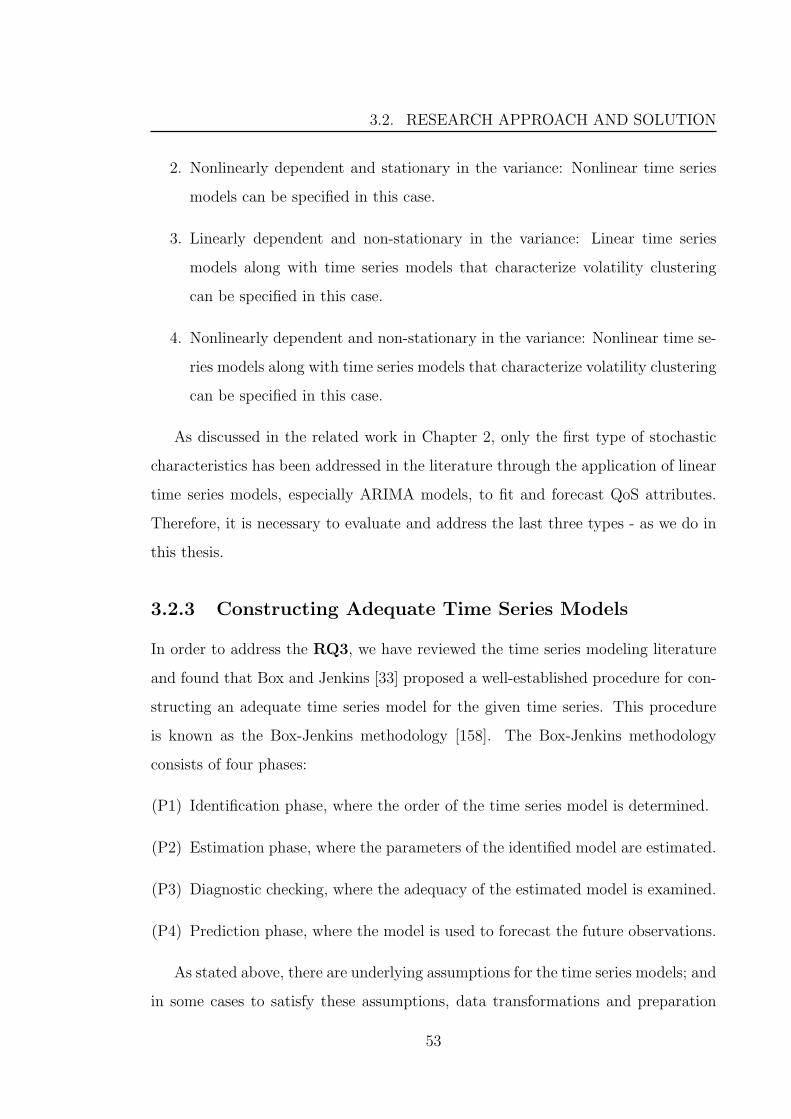
3.2. RESEARCH APPROACH AND SOLUTION
2. Nonlinearly dependent and stationary in the variance: Nonlinear time series
models can be specified in this case.
3. Linearly dependent and non-stationary in the variance: Linear time series
models along with time series models that characterize volatility clustering
can be specified in this case.
4. Nonlinearly dependent and non-stationary in the variance: Nonlinear time se-
ries models along with time series models that characterize volatility clustering
can be specified in this case.
As discussed in the related work in Chapter 2, only the first type of stochastic
characteristics has been addressed in the literature through the application of linear
time series models, especially ARIMA models, to fit and forecast QoS attributes.
Therefore, it is necessary to evaluate and address the last three types - as we do in
this thesis.
3.2.3 Constructing Adequate Time Series Models
In order to address the RQ3, we have reviewed the time series modeling literature
and found that Box and Jenkins [33] proposed a well-established procedure for con-
structing an adequate time series model for the given time series. This procedure
is known as the Box-Jenkins methodology [158]. The Box-Jenkins methodology
consists of four phases:
(P1) Identification phase, where the order of the time series model is determined.
(P2) Estimation phase, where the parameters of the identified model are estimated.
(P3) Diagnostic checking, where the adequacy of the estimated model is examined.
(P4) Prediction phase, where the model is used to forecast the future observations.
As stated above, there are underlying assumptions for the time series models; and
in some cases to satisfy these assumptions, data transformations and preparation
53

CHAPTER 3. RESEARCH METHODOLOGY
activities are needed. Consequently, a preliminary phase of data preparation (P0)
is added to the Box-Jenkins methodology resulting in five phases [137]. The process
of these five phases is depicted in Figure 3.1.
Identify
Adequate
Model
Original
Time Series
Assumptions
Satisfied?
Estimate
Identified
Model
Compute
Forecasts
Diagnostics
OK?
Transformations
Yes
Yes
No No
(P0)
(P1) (P2)
(P3)
(P4)
Figure 3.1: Box-Jenkins procedure for constructing adequate time series model
It is clear from Figure 3.1 that the Box-Jenkins procedure involves manually
identifying a model, estimating its parameters, and checking its adequacy. If this
model is not adequate, it goes back to the identification phase and another model is
re-identified. This process is a time-consuming iterative cycle of identification, esti-
mation, checking and re-identification, which is infeasible if automated runtime QoS
forecasting is required. Therefore, this research project builds on the Box-Jenkins
methodology and proposes a parallelized procedure for constructing an adequate
time series model, as depicted in Figure 3.2. This proposed procedure based on
statistical methods identifies and estimates a set of time series models which can
be used to fit the QoS data under analysis. It then checks the diagnostics of the
estimated models and selects the best one based on an information criterion [1].
The main goal of the proposed procedure is to solve the iterativeness and human in-
tervention issues in order to automatically and quickly construct the adequate time
series model and forecast the future values of the given QoS time series dataset.
As explained in Figure 3.2, the proposed procedure consists of six phases:
(P1) Preliminary phase (data preparation): The underlying assumptions of time se-
54

3.2. RESEARCH APPROACH AND SOLUTION
ries models are verified, and if they are not satisfied some data transformations
are performed.
(P2) Identification phase: A set of adequate time series models is identified based on
auto-correlation function (ACF) and partial auto-correlation function (PACF)
[33,214].
(P3) Estimation phase: Parameters of the identified models are estimated using one
of the well-established statistical estimation methods such as the maximum
likelihood estimation method [4,38].
(P4) Diagnostics phase: Adequacy of the estimated models is examined in terms of
various diagnostic aspects.
(P5) Best model selection phase: The best model among the estimated and exam-
ined ones is selected based on an information criterion [1].
(P6) Prediction phase: The selected model is used to forecast the future values of
the QoS data under analysis.
Collected
QoS Data
(P3)
Estimate Identified
Models
(P4)
Check Diagnostics
of The Models
(P5)
Select The Best
Model
(P1)
Check & Satisfy
Assumptions
(P2)
Identify Adequate
Models
(P6)
Compute ForecatsForecasts
Figure 3.2: Proposed procedure for constructing adequate time series model
Regardless of the class of time series models, this procedure will be used as a base
algorithm in this work to automatically construct the adequate time series model.
Moreover, it is worth mentioning that more phases can be added to this procedure
55

CHAPTER 3. RESEARCH METHODOLOGY
depending on the time series model under construction. For example, if the time
series model requires initial values for specific parameters before the estimation
phase, a new phase before the estimation phase could be added to specify the initial
values for those parameters. In other words, the proposed procedure can be adopted
with some modifications to the given time series model based on its assumptions
and requirements.
3.2.4 Evaluating Adequacy and Forecasting Accuracy
The stochastic characteristics of the given QoS data change over time, which implies
that the adequacy and forecasting accuracy of the constructed time series model need
to be continuously evaluated at runtime in order to enable accurate QoS forecasting.
Statistically, the predictive residuals of an adequate time series model should fluctu-
ate around zero, and recent changes in the underlying QoS data will be immediately
reflected in these predictive residuals by introducing a positive or negative drift.
Therefore, the adequacy of the constructed time series model can be continuously
evaluated by monitoring the predictive residuals and detecting changes in their level.
In statistics literature, statistical control charts are considered as an efficient
technique for online monitoring and detecting changes in a given process [78,95,157,
220]. The main idea of these control charts is constructing a center line (CL), which
represents the average value of the quality characteristic, and two other horizontal
lines called the upper control limit (UCL) and the lower control limit (LCL). These
control limits are chosen so that if the process is in-control, which means there is
no change or shift in the process, nearly all of the values will fall between them.
However, a value that falls outside of the control limits is taken as a signal that a
change has occurred, the process is out-of-control, and investigation and corrective
action are required.
In particular, researchers [95,157] report that the cumulative sum (or CUSUM)
control charts proposed originally by Page [174] are more effective than other exist-
ing charts, e.g. Shewhart charts [210], for quickly detecting small process changes.
56

3.2. RESEARCH APPROACH AND SOLUTION
Furthermore, CUSUM are good candidate for situations where an automatic mea-
surement is economically feasible [95]. Therefore, this research project will adopt the
CUSUM chart to continuously monitor the predictive residuals of the constructed
time series model in order to constantly evaluate its adequacy.
Regarding evaluating the forecasting accuracy, there are several accuracy metrics
that can be used, which are summarised in the following.
• Mean squared error: Suppose the time series model is fitted to a QoS data
of size n observations, yt; and the predicted values, yt, have been obtained.
Mean squared error (MSE) can be computed as follows:
MSE =1
n
n∑t=1
[yt − yt]2 (3.1)
In order to ease the comparison, MSE can be normalized by the deviation from
the average of past values, i.e. [yt − y] and y is the average of past values.
Therefore, relative squared error (RSE) can be computed as follows:
RSE =n∑t=1
[yt − yt]2
[yt − y]2(3.2)
• Root mean squared error: As the unit of the MSE metric is the squared unit
of the original QoS data, root mean squared error (RMSE) can be obtained
to have the same unit of the original QoS data as follows:
RMSE =√MSE =
√√√√ 1
n
n∑t=1
[yt − yt]2 (3.3)
Similarly to MSE, Relative root squared error (RRSE) can be computed as
follows:
RRSE =√RSE =
√√√√ n∑t=1
[yt − yt]2[yt − y]2
(3.4)
57
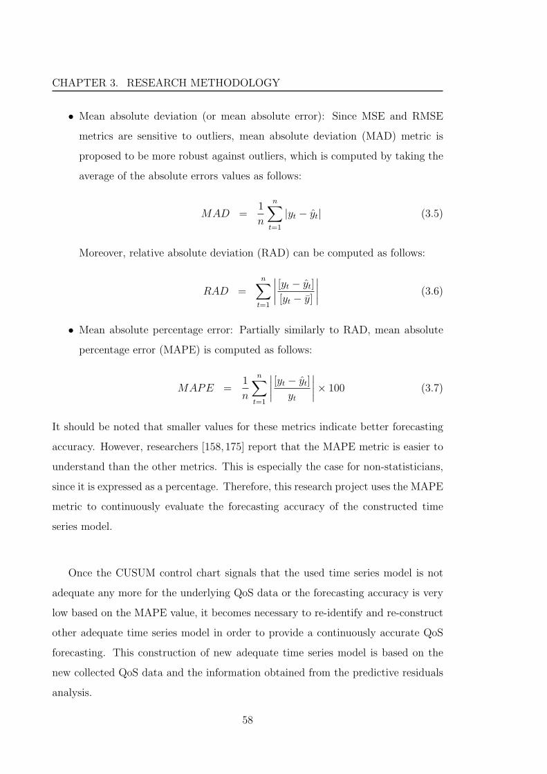
CHAPTER 3. RESEARCH METHODOLOGY
• Mean absolute deviation (or mean absolute error): Since MSE and RMSE
metrics are sensitive to outliers, mean absolute deviation (MAD) metric is
proposed to be more robust against outliers, which is computed by taking the
average of the absolute errors values as follows:
MAD =1
n
n∑t=1
|yt − yt| (3.5)
Moreover, relative absolute deviation (RAD) can be computed as follows:
RAD =n∑t=1
∣∣∣∣ [yt − yt][yt − y]
∣∣∣∣ (3.6)
• Mean absolute percentage error: Partially similarly to RAD, mean absolute
percentage error (MAPE) is computed as follows:
MAPE =1
n
n∑t=1
∣∣∣∣ [yt − yt]yt
∣∣∣∣× 100 (3.7)
It should be noted that smaller values for these metrics indicate better forecasting
accuracy. However, researchers [158, 175] report that the MAPE metric is easier to
understand than the other metrics. This is especially the case for non-statisticians,
since it is expressed as a percentage. Therefore, this research project uses the MAPE
metric to continuously evaluate the forecasting accuracy of the constructed time
series model.
Once the CUSUM control chart signals that the used time series model is not
adequate any more for the underlying QoS data or the forecasting accuracy is very
low based on the MAPE value, it becomes necessary to re-identify and re-construct
other adequate time series model in order to provide a continuously accurate QoS
forecasting. This construction of new adequate time series model is based on the
new collected QoS data and the information obtained from the predictive residuals
analysis.
58

3.3. EVALUATION STRATEGY
3.2.5 Expected Outcome of Addressing Research Questions
The expected outcome of addressing the aforementioned research questions will be a
collection of QoS characteristic-specific automated forecasting approaches that used
together will be able to fit different dynamic behaviors of QoS attributes and fore-
cast their future values. In other words, each one of these forecasting approaches
will be expected to be able to fit only a specific type of stochastic characteristics
of QoS attributes out of the four combinations mentioned above in Section 3.2.2.
For example, one approach will be for fitting and forecasting nonlinearly dependent
QoS attributes and another for fitting and forecasting linearly dependent QoS at-
tributes with volatility clustering. Consequently, this set of forecasting approaches
will constitute a general automated forecasting approach for QoS attributes.
3.3 Evaluation Strategy
Various accuracy and performance aspects of the proposed forecasting approaches
need to be investigated and evaluated. To achieve this, the forecasting approaches
will be applied to various QoS datasets of real-world Web services belonging to
different applications and domains. These real-world QoS datasets will be collected
as discussed and planned in Section 3.2.1.
More specifically, the accuracy of the proposed forecasting approaches can be
classified into two types: (1) The accuracy of forecasting QoS values, and (2) The
accuracy of forecasting potential violations of QoS requirements. First, the accuracy
of forecasting QoS values can be measured by the MAPE metric, as discussed in
the previous section. On the other hand, the accuracy of forecasting potential QoS
violations can be measured and evaluated by proposing contingency table-based met-
rics. Before introducing these metrics, it is worth mentioning that the contingency
table has four cases which are the basis for the proposed metrics. These cases are:
• True positive (TP): A violation was forecasted, and an actual violation oc-
curred.
59

CHAPTER 3. RESEARCH METHODOLOGY
• False positive (FP): A violation was forecasted, but no actual violation oc-
curred.
• True negative (TN): A non-violation was forecasted, and no actual violation
occurred.
• False negative (FN): A non-violation was forecasted, but an actual violation
occurred.
Based on these cases, contingency table-based metrics [147, 148, 199] can be de-
fined and computed as follows:
• Precision value (PV): Is the percentage of correctly forecasted violations to
total forecasted violations, which is computed as follows:
PV =TP
TP + FP× 100 (3.8)
• Recall value (RV): Is the percentage of correctly forecasted violations to total
actual violations, which is computed as follows:
RV =TP
TP + FN× 100 (3.9)
• False positive rate (FPR): Is the percentage of incorrectly forecasted violations
to the number of all non-violations, which is computed as follows:
FPR =FP
FP + TN× 100 (3.10)
• Negative predictive value (NPV): Is the percentage of correctly forecasted non-
violations to total forecasted non-violations, which is computed as follows:
NPV =TN
TN + FN× 100 (3.11)
• Specificity value (SV): Is the percentage of correctly forecasted non-violations
60

3.3. EVALUATION STRATEGY
to total actual non-violations, which is computed as follows:
SV =TN
TN + FP× 100 (3.12)
• F-measure value (FMV): Is the weighted harmonic mean of precision value
(PV) and recall value (PV), which is computed as follows:
FMV =(1 + β2)·PV ·RVβ2·PV +RV
, (3.13)
where β ≥ 0 is the weighted parameter.
• Accuracy value (AV)1: Is the percentage of all correctly forecasted viola-
tions and non-violations to the number of all forecasted violations and non-
violations, which is computed as follows:
AV =TP + TN
TP + FP + TN + FN× 100 (3.14)
By relating these metrics to the adaptation of Web services or service-based
systems which is discussed in Chapter 2, precision value can be used to evaluate
incorrectly forecasted needs for adaptation, i.e. unnecessary adaptations [148]. Ac-
cordingly, a higher precision value means fewer false alarms of violations and thus
implies less unnecessary adaptations. Similarly, recall value can be related to missed
adaptations, where higher values means more actual violations being forecasted and
thus implies fewer missed adaptations [148]. Consequently, the proposed forecast-
ing approaches should achieve high values of precision and recall. However, re-
searchers [134,148,199] report a trade-off between precision and recall to the extent
that improving precision, i.e. reducing the number of false positives, might result in
worse recall, i.e. increasing the number of false negatives. In order to consider the
trade-off between precision and recall in one metric, the F-measure value has been
proposed as a weighted harmonic mean of precision and recall [125, 134, 199, 245].
1As a note on terminology, “accuracy” is used as a generic term in this thesis as long as it isnot referred explicitly as a contingency table-based metric.
61

CHAPTER 3. RESEARCH METHODOLOGY
Indeed, the F-measure value is balanced when the weighted parameter β = 1, and
otherwise it favors precision when β < 1 and recall when β > 1 [148].
Similarly to the use of recall value, the negative predictive value can be used
to evaluate missed adaptations, because a higher value of the negative predictive
value means more actual violations being forecasted and thus implies fewer missed
adaptations [147, 148]. Additionally, similar to the precision value, specificity value
can be related to unnecessary adaptations, and a higher value of specificity means
less false alarms of violations and thus implies fewer unnecessary adaptations [147,
148]. Finally, accuracy value takes into account all the cases of violations and non-
violations, which can be used as a general metric for the accuracy of forecasting QoS
violations. However, Salfner et al. [199] do not recommend using this metric as a sole
indicator for evaluating the accuracy of forecasting QoS violations. Salfner et al.’s
justification is that the forecasting approach can achieve a higher accuracy value
despite it might not catch any actual violation, because the failures or violations
are usually rare events. Moreover, Metzger et al. [148] point out that in the case of
service-based systems the majority of QoS observations will indicate non-violations,
and as a result the negative predictive value, specificity, and accuracy metrics might
always be high. This is why the precision and recall metrics (or, as a single metric,
F-measure value) is sufficient to evaluate the forecasting accuracy of these QoS
datasets.
Based on this discussion of the introduced metrics and their relation to the
adaptation of service-based systems, it can be concluded that metrics that relate to
unnecessary adaptations or missed adaptations and cover all the four cases of the
contingency table should be considered in order to achieve a comprehensive picture
of evaluating forecasting accuracy [147, 148]. Therefore, this research project will
consider the negative predictive value, specificity, F-measure value, and accuracy
metrics to evaluate the accuracy of forecasting QoS violations because they relate
to unnecessary adaptations and missed adaptations as well as cover all those four
cases of the contingency table.
62

3.4. SUMMARY
Regarding the performance of the proposed forecasting approaches, it can be
simply measured in two ways, namely the time required to construct the time se-
ries model and the time taken to use the time series model. These times may be
quite different. In addition, the time series model may only need to be constructed
occasionally, whereas it will be continuously used. Obviously, the less time required
to construct or use the time series model the higher performance the forecasting
approach achieves. The accuracy and performance of the proposed forecasting ap-
proaches will be compared to those of the baseline ARIMA models in order to
evaluate the extent of any relative improvement of those proposed forecasting ap-
proaches. In addition, non-parametric tests will be used to evaluate the significance
of any difference in accuracy or performance.
3.4 Summary
This chapter first presented the challenges, formulated as research questions, of
developing a general automated forecasting approach for QoS attributes. These
challenges include evaluating the QoS stochastic characteristics, specifying the class
of adequate time series models, constructing the specified time series models, and
finally evaluating the adequacy and accuracy of the constructed time series model.
The chapter then introduced the research approach that will be applied to address
these formulated research questions, aiming to achieve the overall research goal.
Finally, it discussed the evaluation strategy that will be used to evaluate the accuracy
and performance of the contributions in this thesis.
63

CHAPTER 3. RESEARCH METHODOLOGY
64

Chapter 4
Evaluation of Stochastic
Characteristics of QoS Attributes
In order to propose an efficient forecasting approach that is able to adequately fit
a dynamic behavior of QoS attributes and accurately forecast their future values, it
is required in the beginning to identify and evaluate the stochastic characteristics
of these QoS attributes. This is because the proposed forecasting approach has to
be constructed based on the QoS stochastic characteristics. As discussed in Chap-
ter 3, these QoS stochastic characteristics include probability distribution, serial
dependency, stationarity (in the mean and variance), and nonlinearity.
The evaluation of these stochastic characteristics has to be based on real-world
QoS datasets to represent real characteristics. However, as mentioned in Chapter
3, there is a lack of existing real-world QoS datasets that can be used to evaluate
the QoS stochastic characteristics, and then enable the construction of adequate
QoS forecasting approach. In order to address this problem and achieve the current
research goal, several real-world Web services are invoked, and their response time
and time between failures are computed.
This chapter is organized as follows. Section 1 explains how the real-world Web
services are invoked, and how their response time and time between failures datasets
are computed. After that, Section 2 introduces each QoS stochastic characteristic,
65

CHAPTER 4. EVALUATION OF STOCHASTIC CHARACTERISTICS OFQOS ATTRIBUTES
followed by a discussion of how it can be evaluated using statistical tests/methods.
This is achieved along with a running example of evaluating the stochastic char-
acteristics of response time and time between failures of real-world Web service in
order to explain how the evaluation is conducted. Finally, Section 3 discusses the
results of evaluating stochastic characteristics of the collected response time and
time between failures datasets.
4.1 Invocation of Real-World Web Services
Real-world Web services can be monitored from server-side and client-side as dis-
cussed in Chapter 2. Although server-side monitoring might provide accurate QoS
measures, it requires access to the actual service implementation which is not al-
ways possible [153]. In contrast, client-side monitoring is independent of the service
implementation; however, the collected QoS measures might be affected by different
uncontrolled factors such as networking performance. Because in this thesis several
real-world Web services are planned to be invoked and the access to their actual
implementation is difficult, the client-side invocation and monitoring approach is
adopted in the current research work.
Technically, in order to invoke real-world Web services some steps have to be
followed, which include discovering real-world Web services, getting their WSDL
files, and finally generating client-side invocation codes. These steps are discussed
in some details in the following.
Discovering Real-World Web Services
Many real-world public Web services are available on the Internet, and they can be
discovered form different sources such as:
• XML-based UDDI (Universal Description, Discovery and Integration) reg-
istries, which enable companies to publish and crawl public web services on
the Internet.
66

4.1. INVOCATION OF REAL-WORLD WEB SERVICES
• Web service search engines, which index public Web services and enable users
to perform search queries to find them. Examples of these search engines are
seekda.com, esynaps.com and cowebservices.com.
• Web service portals such as remotemethods.com, wsindex.org, xmethods.net,
and webservicelist.com.
Currently, based on seekda.com counter report [207], there are totally 28,606
real-world Web services which are publicly available on the Internet with WSDL
documentations.
Getting Web Services WSDL Files and Generating Invocation Codes
To get the Web services WSDL files, it is required to establish HTTP connections
to the WSDL addresses. Once these HTTP connections are successfully established
without failures, WSDL files can be downloaded. Using the obtained WSDL files,
Axis22 can be employed to generate client-side invocation codes for those available
Web services.
Collected Response Time and Time Between Failures Datasets
With the assistance of the tool Ws-dream [256], 800 real-world Web services have
been selected randomly, without any personal selection judgment. Then, each one of
these Web services has been invoked sequentially for about 1,000 times and its non-
functional performance has been recorded, which includes response time, response
data size, response HTTP code, and failure message. The response time is computed
by measuring the time taken between sending a request to a service and receiving a
response. In the current case of invoking real-world Web services, the response time
is assumed to be independent of the input data values.
Using the Web service response HTTP codes, it can be detected whether the
Web service invocation has succeeded or failed; and if it fails, what is the failure
2http://ws.apache.org/axis2
67

CHAPTER 4. EVALUATION OF STOCHASTIC CHARACTERISTICS OFQOS ATTRIBUTES
type. Generally, HTTP code 200 reports that the invocation is successful, which
means that the request is processed under stated conditions and the response is
received in a specified time interval [116]. However, other codes (and exceptions)
indicate to several types of Web service invocation failures [256]. These types of
invocation failures are presented in Table 4.1, and discussed briefly in the following:
• Bad Request: The HTTP protocol is not completely respected by the client
request which causes that the Web server is confused and unable to fully
understand the request.
• Internal Server Error: An unexpected condition is encountered by the Web
server, which prevents fulfilling correctly the client request.
• Bad Gateway: An invalid response from an upstream server is received by a
gateway or proxy server.
• Service Unavailable: Because of a temporary maintenance or overloading of
the Web server, the HTTP request is not handled and processed by the service.
• Unknown Host: The host’s IP address can not be determined.
• Connection Refused: While a socket attempts to connect to a remote address,
an error occurs. This means the connection is remotely refused.
• Connection Reset: A socket is unexpectedly closed from the server-side.
• Connect Timed Out: A timeout occurs on a socket connect.
• Read Timed Out: A timeout occurs on a socket read.
These failures are caused by different Web service invocation errors which can
be classified as:
• Server-side errors
• Network connection problems
• Socket exceptions
68

4.1. INVOCATION OF REAL-WORLD WEB SERVICES
Failure Message Description
java.io.IOException: Server returned HTTP response code: 400 for URL Bad request
java.io.IOException: Server returned HTTP response code: 500 for URL Internal server error
java.io.IOException: Server returned HTTP response code: 502 for URL Bad gateway
java.io.IOException: Server returned HTTP response code: 503 for URL Service is unavailable
java.net.UnknownHostException Unknown host
java.net.ConnectException: Connection refused Connection refused
java.net.SocketException: Connection reset Connection reset
java.net.SocketTimeoutException: connect timed out connect timed out
java.net.SocketTimeoutException: Read timed out Read timed out
Table 4.1: Failure types of Web services invocations
The failures that are caused by the server-side errors include bad request, in-
ternal server error, service unavailable, connection reset, and connection refused.
In addition, network connection problems cause other failures such as bad gateway
and unknown host. Besides all these failures, timeout failures, which include con-
nect time out and read time out, are caused by socket exceptions during socket
connection and socket read respectively. It is worth mentioning that, in this work
the Web service invocations have been configured with a default timeout setting of
Axis2, which is 20 seconds. Of course, by setting different timeout value the number
of timeout failures may vary.
Indeed, 1,000 invocations of a Web service can not guarantee getting enough
number of failures that can be used to compute time between failures datasets.
Therefore, 325 Web services out of the 800 real-world Web services have been se-
lected to be invoked every 10 minutes for 150 days. The main criterion of selecting
these Web services is that they are mostly used in practice according to seekda.com
evaluation. The description of a sample of these selected Web services is reported in
Table 4.2, and more details are introduced in Appendix A. It is important to note
that the time between invocations is selected to be 10 minutes only to help collect-
ing enough number of failures and does not have any effect on the response time.
Indeed, the Web service’s response time level from the client’s point of view is made
69

CHAPTER 4. EVALUATION OF STOCHASTIC CHARACTERISTICS OFQOS ATTRIBUTES
up of many aspects such as network performance, current load from other clients,
complexity of data requests, and load of the server from other Web services. Using
the failures data obtained from this long time-based invocation, the time between
failures datasets have been computed without taking into account the distinction
between the failures types presented in Table 4.1. Thus, the current research consid-
ers the computed response time and time between failures datasets as the main QoS
measures that are used in this thesis to evaluate the QoS stochastic characteristics of
Web services, and then used in proposing and evaluating an automated forecasting
approach for QoS attributes.
4.2 QoS Stochastic Characteristics and How to
Evaluate
This section introduces the key QoS stochastic characteristics, which include prob-
ability distribution, serial dependency, stationarity, and nonlinearity, and discusses
how to evaluate each one using statistical methods/tests. In the beginning, it in-
troduces the fitting of probability distributions to QoS datasets using the maximum
likelihood estimation method [4, 38] and how to achieve normality using the power
transformation method [32]. Then, the section discusses the QoS serial dependency
and how it can be evaluated using the runs test [233]. After that, it introduces
the QoS stationarity concept, which is differentiated into two types; stationarity in
the mean and stationarity in the variance. It then discusses how these two types
of stationarity can be evaluated using the KPSS test [115] and Engle test [115],
respectively. Finally, the section introduces the QoS nonlinearity and how it can
be evaluated using the Hansen test [90]. This is achieved along with evaluating
the stochastic characteristics in detail on the running example of the response time
and time between failures datasets of “GlobalWeather”3 service. This Web service
provides the current weather with additional information for major cities around
3http://www.webservicex.com/globalweather.asmx
70

4.2. QOS STOCHASTIC CHARACTERISTICS AND HOW TO EVALUATE
WSid WS Name Description Provider Name
WS1 StockQuote Reports stock quotations for a companyby using provided stock symbol.
WebserviceX.NET
WS2 YahooQuoteWebService Gets delayed stock information from Ya-hoo by using provided stock symbol.
datasprings.com
WS3 HolidayService Calculates national holidays for the pro-vided country code.
holidaywebservice.com
WS4 PhoneNotify Delivers on-demand voice notifications,including alerts and two-way interactivevoice messaging.
CDYNE Corporation
WS5 GetAuditInfo Gets some infromation about executingan operation of a system as well as usersinformation such as user, name, pass-word, date, and time.
topfo.com
WS6 SmsSend2 Sends two-way SMS messages. utnet.cn
WS7 Research Research service in Microsoft Office 2003provides a definition, a synonym, factsabout a company’s finances, an encyclo-pedia article, or other types of informa-tion from the Web.
microsoft.com
WS8 TiempoService Used by transportesjoselito.com to getthe time.
transportesjoselito.com
WS9 Doc Used by shuaiche.com to implement a setof document style interop operations.
shuaiche.com
WS10 Service1 Used by visualprog.cz as authenticationservice in order to allow clients to get aglobally unique identifier (GUID) fromthe database by using their login namesand passwords.
visualprog.cz
WS11 AjaxWS Used by cnblogs.com to collect userscomments and questions.
cnblogs.com
WS12 BookStoreService Provides the list of the books accordingto author, title, price and chckes for theiravailability.
tempuri.org
WS13 ValidateCodeWS Supports codes validation including Chi-nese letters, numbers, images and multi-media.
webxml.com.cn
WS14 TraditionalSimplifiedWS Provides conversion of simplified Chinesefrom/to traditional Chinese.
webxml.com.cn
WS15 SharepointEmailWS Is sharepoint email integration Web ser-vice that creates, modefies, and deletescontacts and groups details.
perihel.hr
Table 4.2: Examples of the monitored real-world Web services
71

CHAPTER 4. EVALUATION OF STOCHASTIC CHARACTERISTICS OFQOS ATTRIBUTES
the world.
4.2.1 Probability Distribution and Transformation to Nor-
mality
Although it is known that QoS attributes are probabilistic and can be characterized
by specific probability distributions such as gamma and weibull distributions [25,151,
205], it is required to evaluate these distributions based on real-world QoS datasets.
This evaluation of QoS probability distributions is important to guide in selecting
the suitable statistical method/test to study and analyze the given QoS attributes,
such as proposing a forecasting model to fit response time measures and forecast
their future values. Consequently, one of the current research tasks is to evaluate
the probability distributions of QoS attributes, especially response time and time
between failures.
Generally, there are different techniques for fitting probability distribution such
as the maximum likelihood estimation method [4,38], least square estimation method
[185], method of L-moments [101], and method of moments [61]. However, the
maximum likelihood estimation method is the most commonly used because of the
general good properties of its estimates such as unbiasedness, consistency, efficiency,
and sufficiency [76]. Therefore, this research project adopts this estimation method
for fitting the probability distribution of QoS attributes.
For explanation, the likelihood is the probability of the data point, yt, under
the hypothesis that the data have a specific probability distribution. For a set of N
points yt which are obtained from a common distribution, the likelihood function
can be written as:
L(yt; β) = P (y1; β)P (y2; β) . . . P (yN ; β) =N∏t=1
P (yt; β) (4.1)
where β is a vector of parameters of the probability distribution. By maximizing
the likelihood function with respect to the distribution parameters, β, the maximum
72

4.2. QOS STOCHASTIC CHARACTERISTICS AND HOW TO EVALUATE
likelihood solution is obtained. In practice, it is usually easy to maximize the log
likelihood function, rather than the likelihood function itself, which converts the
product in equation 4.1 into a sum as follows:
lnL(yt; β) = lnN∏t=1
P (yt; β) =N∑t=1
lnP (yt; β) (4.2)
Assuming that β is the parameters’ estimate that maximizes the log-likelihood func-
tion, then β is called the maximum likelihood estimate and lnL(yt; β) is called the
maximized log-likelihood function.
The planned method for fitting the probability distributions consists of two steps.
• First, a number of probability distributions for the given QoS data is fitted
using the maximum likelihood estimation method (MLE).
• Then, the adequate distribution, which is well fitting the QoS data, is selected
using Akaike’s information criterion (AIC) [1]:
AIC = 2k − 2ln(L) (4.3)
where k is the number of parameters in the fitted distribution, and ln(L) is
the maximized log-likelihood function for the fitted distribution. The best
adequate distribution for the given QoS data is the one that has the minimum
AIC value.
As discussed in Chapter 3, because response time and time between failures
datasets are theoretically asymmetrically distributed [25, 151, 192, 205], the prob-
ability distributions considered in the current evaluation are skewed distributions
which include exponential, gamma, weibull, log-logistic, and non-central student’s t
(or simply non-central t). In addition, to check whether a symmetric distribution
can characterize these QoS attributes, the normal distribution is added in the eval-
uation to all be six fitted probability distributions. Examples of these distributions
are depicted in Figure 4.1.
73

CHAPTER 4. EVALUATION OF STOCHASTIC CHARACTERISTICS OFQOS ATTRIBUTES
0 2 4 6 8 10
0.0
0.2
0.4
0.6
(a) Exponential
0 2 4 6 8 10
0.0
0.2
0.4
0.6
0.8
(b) Gamma
0 2 4 6 8 10
0.0
0.1
0.2
0.3
(c) Weibull
0 2 4 6 8 10
0.0
00.0
50.1
00.1
5
(d) Log-logistic
0 2 4 6 8 10
0.0
00.0
50.1
00.1
50.2
00.2
5
(e) Non-Central t
0 2 4 6 8 10
0.0
0.1
0.2
0.3
0.4
(f) Normal
Figure 4.1: Examples of fitted probability distributions
Most of the powerful (parametric) statistical tests, methods, and models assume
that the data is normally distributed. This assumption is reasonable in the cases
where the data observations follow the normal distribution. However, in the cur-
rent case, the QoS attributes, namely response time and time between failures, are
expected to be mostly asymmetrically and non-normally distributed. Therefore, it
is required to modify (statistically called “transform”) the QoS data to be normally
(or at least approximately normally) distributed to make the using of those statisti-
cal methods based on normal assumption more appropriate. Power transformation,
especially Box-Cox transformation [32], is the most commonly used technique to
transform the data to be normally distributed. By way of explanation, the Box-Cox
transformation yt(λ) of the data zt is given as follows:
yt(λ) =
(zλt −1)
λif λ 6= 0
log zt if λ = 0
(4.4)
74

4.2. QOS STOCHASTIC CHARACTERISTICS AND HOW TO EVALUATE
where λ is the transformation parameter and its value is chosen to reduce the vari-
ation of the data zt in order to achieve normality.
In this work, because forecasting approaches are proposed based on time series
models that assume normality, the Box-Cox transformation is applied to transform
the response time and time between failures data to be normally distributed. More-
over, it is worth mentioning that the anti-transformation can be applied to get the
original data from the transformed one. For instance, assume the log transforma-
tion is used to transform the response time data to be normally distributed, and
thus the forecasting model is applied to the transformed response time to forecast
future values. The forecasting of original response time can be obtained by applying
exponential transformation for the forecasted log response time values.
Example . Initially, the descriptive statistics of the response time and time
between failures of the “GlobalWeather” service are presented in Table 4.3. From
this Table, it can be seen that the “GlobalWeather” service can respond on average
in 583.5 ms with standard deviation is about 51 ms. Based on the first and third
quartiles values (Q1 and Q3), the service’s response time is between 563 ms and 594
ms in 50% of the invocations. It is worth noting that the mean of response time
(= 583.5) is greater than the median (= 579.0) because the response time data is
(positively) skewedly distributed. This fact is visualized by the histogram depicted
in Figure 4.2a.
QoS Min Q1 Median Mean St.D. Q3 Max
RT (ms) 437.0 563.0 579.0 583.5 51.1 594.0 797.0
TBF (min) 20.0 220.0 480.0 557.0 455.0 730.0 2010.0
Table 4.3: Descriptive statistics of response time (RT) and time between failures(TBF) of GlobalWeather service
Regarding the time between failures measure of the “GlobalWeather” service,
Table 4.3 shows that the mean time between failures (MTBF) is 557 minutes (for
request rate is one request per 10 minutes), which implies that the service reliability
75

CHAPTER 4. EVALUATION OF STOCHASTIC CHARACTERISTICS OFQOS ATTRIBUTES
is on average about 98.2%. In addition, values of the Q1 and Q3 report that 50% of
the time between failures are between 220 minutes and 730 minutes, which indicates
that the time between failures is highly dynamic. Moreover, the large difference
between the mean and median values implies that the time between failures measure
is very (positively) skewedly distributed, as depicted in Figure 4.2c.
Response Time (ms)
Fre
qu
en
cy
500 600 700 800
05
00
10
00
15
00
20
00
(a) Response Time (ms)
Transformed Response Time
Fre
qu
en
cy
2.55 2.60 2.65 2.70 2.75 2.80 2.85
05
00
10
00
15
00
20
00
25
00
(b) Transformed Response Time
TBF (min)
Fre
qu
en
cy
0 500 1000 1500 2000
05
10
15
20
(c) TBF (min)
Transformation of TBF
Fre
qu
en
cy
0 5 10 15 20 25 30 35
05
10
15
20
25
30
(d) Transformed TBF
Figure 4.2: Histograms of response time, time between failures (TBF), and theirtransformations of GlobalWeather service
To fit the six probability distributions for the response time and time between
failures data of the GlobalWeather service, first the MLE method is used to fit
the distributions, and then the AIC measure is used to select the most adequate
76

4.2. QOS STOCHASTIC CHARACTERISTICS AND HOW TO EVALUATE
one. From Table 4.4, it can be seen that the most adequate distribution to fit the
GlobalWeather’s response time is non-central t, which has the minimum AIC value.
On the other hand, the time between failures data can be well fitted by weibull
distribution. However, it is worth noting that the maximized log-likelihood function
and AIC values of the fitted three distributions exponential, gamma, and weibull
are very similar, which means that in some cases more than one distribution can be
used to fit the same QoS data. Actually, this is driven from the statistical fact that
for specific values of the different distributions’ parameters, these distributions can
be equivalent [113].
Fitting Probability Distribution
QoS Measure Exponential Gamma Weibull Log-logistic Non-central t Normal
RTMLL -7368.99 -5347.61 -5492.27 -5441.75 -5174.28 -5353.07
AIC 14739.98 10699.23 10988.55 10889.49 10354.55 10710.14
TBFMLL -507.02 -505.65 -505.14 -515.03 -525.85 -528.40
AIC 1016.05 1015.30 1014.27 1034.06 1057.69 1060.80
Table 4.4: Maximized log-likelihood (MLL) and AIC values of fitting probabilitydistributions
Visualization can be used as a simple method to illustrate the fitting results. For
example, by comparing the histograms of response time (in Figure 4.2a) and time
between failures data (in Figure 4.2c) to the simulated examples of non-central t (in
Figure 4.1e) and Weibull distributions (in Figure 4.1c), respectively, it can be seen
that their shapes are similar.
Now based on the fitting results, the GlobalWeather’s response time and time
between failures datasets are not normally distributed; and to apply the statistical
methods which assume normality to analyze these datasets, the Box-Cox transfor-
mation can be used to transform them to be normally distributed. By applying the
Box-Cox transformation to the response time data, it is reported that the trans-
formation parameter of value “0.156” transforms the data to be (approximately)
normally distributed as depicted in Figure 4.2b. On the other hand, time between
77

CHAPTER 4. EVALUATION OF STOCHASTIC CHARACTERISTICS OFQOS ATTRIBUTES
failures is transformed to be (approximately) normally distributed by using trans-
formation parameter of value “0.467”, as presented in Figure 4.2d. /
4.2.2 Serial Dependency
In order for QoS data to be effectively characterized and forecasted by using time
series models, it should be serially dependent (autocorrelated over time). This is why
serial dependency characteristic is very important and needs to be evaluated in the
early phase of time series modeling before doing any further data analysis to decide
whether those time series models are suitable to fit QoS data and accurately forecast
future values. There are several well-known statistical tests proposed by Wald and
Wolfowitz [233], Wald and Wolfowitz [234], Moore and Wallis [160], Mann [142],
Daniels [56], and Foster and Stuart [71] to evaluate the serial dependency. The test
proposed by Wald and Wolfowitz [233] is known as the runs test, and it is studied by
David [58], Goodman [81], and Granger [83]. In particular, Granger [83] concludes
that the runs test is both much quicker to apply than other available tests and
appropriate for use with non-stationary data. Therefore, this test is adopted in this
work for evaluating the serial dependency of QoS attributes.
The runs test [77, 233] is used to test the null hypothesis that the elements
of the QoS time series are mutually independent. If this hypothesis is rejected
that means the given QoS data is serially dependent, and time series modeling
can be used to construct a forecasting model for this data. In order to explain
how the runs test works to evaluate the QoS serial dependency, assume there are N
observations of the QoS data, yt for t = (1, . . . , N), and their median is computed;
then the test compares each observation to the median value and creates a random
variable of symbols takes values positive (+) or negative (-) according to whether the
observation is larger or smaller than the median value. After that, the test defines
the run as a sequence of identical symbols. The number of runs provides information
that can be used to check whether QoS data is serially dependent; where if there
are few runs, this means the QoS data is most likely dependent and otherwise it is
78

4.2. QOS STOCHASTIC CHARACTERISTICS AND HOW TO EVALUATE
random and independent. Assuming the number of runs is a random variable, R,
with mean and variance can be calculated as follows:
E(R) = (2N1N2
N) + 1, (4.5)
V (R) =2N1N2(2N1N2 −N)
N2(N − 1)(4.6)
where N, N1, and N2 are the total number of QoS observations, positive (+) runs,
and negative (-) runs, respectively. Based on the calculated mean and variance,
the Z statistic can be constructed to test the null hypothesis that the QoS data
is independent against the alternative hypothesis that it is serially dependent, as
follows:
Z =r + h− E(R)√
V (R)(4.7)
where r is the total number of runs, and h equals to 0.5 if (2N1N2 - N) + 1 is greater
than r and otherwise equals to -0.5. At a confidence level 95%, the hypothesis that
QoS data is serially dependent is not rejected if the absolute value of Z is greater
than 1.96.
Example . By applying the runs test to the response time and time between
failures datasets of the GlobalWeather service, the results are obtained and reported
in Table 4.5. From this Table, it can be concluded that these two datasets are serially
dependent, where p-values are less than 0.05. /
QoS Z-Statistic P-Value
RT -3.6058 0.0003
TBF -2.6994 0.0069
Table 4.5: Runs test results for the GlobalWeather’s response time (RT) and timebetween failures (TBF)
79

CHAPTER 4. EVALUATION OF STOCHASTIC CHARACTERISTICS OFQOS ATTRIBUTES
4.2.3 Stationarity
In time series analysis, at each measurement point only one observation is observed
for a variable of interest such as a response time of each service request, which
constructs one realization of data. The mean, variance, and autocorrelations of the
series of interest can be estimated by averaging across the single realization only if
the series is stationary. This is why most time series models assume that the time
series of interest is stationary or has been stationarized.
Theoretically, there are two types of stationarity; strict (or strong) stationarity
and weak stationarity [33]. To explain this concept, assume the joint distribution
function of the N random variables Yt1 , . . . , YtN drawn from the stochastic process
Yt : t = 0,±1,±2, . . . can be written as follows:
FYt1 ,...,YtN (yt1 , . . . , ytN ) = PYt1 ≤ yt1 , . . . , YtN ≤ ytN (4.8)
where yti for i = 1, 2, . . . , N are real numbers. A time series is strongly (or strictly)
stationary if the joint distribution function is the same over time and only depends
on the time difference, which means that:
FYt1 ,...,YtN (yt1 , . . . , ytN ) = FYt1+h ,...,YtN+h(yt1+h , . . . , ytN+h
) (4.9)
where h is any real number represents the time difference. For this strictly sta-
tionary time series, the mean and variance are constants and do not depend on the
time, which implies that µ = E(Yt) and σ2 = E(Yt − µ)2. On the other hand,
the correlation function depends only on the time difference, which means that
ρ(Yt1 , Yt2) = ρ(Yt1+h , Yt2+h) for any time points t1 and t2 and time difference h.
In practice, it is not easy to check for the strict stationarity. Therefore, the
empirical time series analysis is interested into the joint moments rather than the
joint distribution function, and the time series is called weakly stationary of order
n if it has constant joint moments up to order n. For example, in the case of
second order weak stationarity the time series has constant mean and variance, and
80

4.2. QOS STOCHASTIC CHARACTERISTICS AND HOW TO EVALUATE
its autocorrelation function depends only on the time difference. Accordingly, this
explains why this work checks for (weak) stationarity by only testing whether the
time series has constant mean and variance over time. For simplicity, when a time
series has constant mean (no trend) over time, it is called stationary in the mean;
and when it has constant variance (same variation) over time, it is called stationary
in the variance.
4.2.3.1 Stationarity in the Mean
Regarding stationarity in the mean, Dickey-Fuller tests [62, 63, 197] and
Kwiatkowski-Phillips-Schmidt-Shin (KPSS) test [115] are the most commonly
used to check for stationarity in the mean of time series [60,127,136,190]. However,
some researchers [100, 115, 164] report that the Dickey-Fuller tests have low power
against stationarity, i.e. they highly fail to accept the alternative hypothesis
of stationarity for actual stationary time series, as confirmed by the findings of
empirical studies [60, 164]. Because the KPSS test tackles this problem [115], it is
preferred to be adopted in this research project.
The KPSS test evaluates the null hypothesis that the QoS data is stationary
in the mean. To illustrate the general idea of KPSS test, let yt, for t = 1, . . . ,
N, be the observed QoS time series data for which stationarity is tested. The test
decomposes this QoS series into the sum of three parts, which are:
• A random walk which is modeled as rt = rt−1 + ut, where ut is normally
distributed with mean equals to zero.
• A deterministic trend which is represented as βt.
• A stationary error which is referred as εt.
Then, it constructs a linear regression model as follows:
yt = rt + βt+ εt (4.10)
81

CHAPTER 4. EVALUATION OF STOCHASTIC CHARACTERISTICS OFQOS ATTRIBUTES
To test the stationarity, the test actually assumes the null hypothesis that β = 0.
Under this null hypothesis, the KPSS test statistic can be calculated as:
KPSS = N−2
∑Nt=1 S
2t
σ2(p)(4.11)
where N is number of observations, St is the sum of regression residuals (et’s), and
σ2(p) is a consistent estimator of the variance of et’s which is computed as follows:
σ2(p) =1
N
N∑t=1
e2t +
2
N
p∑j=1
wj(p)N∑
t=j+1
etet−j (4.12)
where wj(p) is a weighting function of the truncation lag p, such as wj(p) = 1 −
j/(p+ 1). The decision of KPSS test is based on the upper tail critical values of the
statistic’s asymptotic distribution, which is given by Kwiatkowski et al. [115].
The rejection of KPSS null hypothesis means that the QoS data is non-stationary,
and therefore a transformation method is required to stationarize this data. One of
the most commonly used method to stationarize the time series data is using the
differencing of the non-stationary time series. For example, let zt be the original
time series which is non-stationary in the mean, has trend over time, as depicted
in Figure 4.3a. It can be transformed into a stationary one yt using the first
difference, i.e. yt = zt− zt−1. The differenced series yt is depicted in Figure 4.3b,
and it is clear that it is stationary in the mean.
4.2.3.2 Stationarity in the Variance
Some statistical tests are proposed by Breusch and Pagan [35], White [238], and
Engle [68] in order to evaluate the stationarity in the variance. However, the Engle’s
test [68] is known with its simplicity [69] and efficiency especially in the availability
of small number of observations [129], which is the reason to be adopted in this
work. Generally, the Engle test [68] is used with the null hypothesis that the QoS
data has constant variance. Technically, the Engle test in the beginning fits the
82

4.2. QOS STOCHASTIC CHARACTERISTICS AND HOW TO EVALUATE
Time Index
zt V
alu
es
0 20 40 60 80 100
50
55
60
65
70
(a) The original time series zt
Time Index
yt V
alu
es
0 20 40 60 80 100
−3
−2
−1
01
23
(b) The differenced time series yt
Figure 4.3: The original nonstationary vs. differenced stationary time series
most adequate autoregressive model for the QoS data yt as:
yt = φ0 +
p∑i=1
φiyt−i + εt, t = 1, 2, . . . , N (4.13)
where φi’s for i = 1, . . . , p are the model coefficients and p is the model order. After
fitting this model, the squared residuals εt2 are computed and fitted by another
autoregressive model as:
εt2 = α0 +
q∑i=1
αiε2t−i + et, t = 1, 2, . . . , N (4.14)
Under the null hypothesis of constant variance, it is expected that all the values
of αi’s to be close to zero, which implies that the squared residuals are not auto-
correlated over time. Therefore, the Engle statistic is computed as NR2, where N
is the number of QoS data observations and R2 is the coefficient of determination
in model 4.14, which measures how well the model fits the squared residuals [158].
Since this statistic asymptotically follows the χ2(q) distribution, the decision of the
test is based on the upper tail critical values of the χ2 distribution [113]. Rejecting
the Engle test’s null hypothesis means that the QoS data has non-constant variance
83

CHAPTER 4. EVALUATION OF STOCHASTIC CHARACTERISTICS OFQOS ATTRIBUTES
over time, which is statistically called volatility clustering (or in short volatility).
Example . The stationarity in the mean of the GlobalWeather’s response time
and time between failures datasets is evaluated by applying the KPSS test, and the
results are depicted in Table 4.6. This Table shows that both response time and time
between failures datasets are non-stationary in the mean, where p-values are less
than 0.05. Then, these datasets are stationarized by using the differencing method,
and then the KPSS test is re-applied. The KPSS test concludes that the differences
of response time and time between failures are stationary (p-values > 0.05). This
result can be illustrated by Figure 4.4. By looking at Figures 4.4a and 4.4c, it can
be seen that the response time and time between failures do not have constant level,
where there is increasing and decreasing trend. However, Figures 4.4b and 4.4d
show that the changes of response time and time between failures over time, which
are computed by the differencing method, have constant level.
QoS RT D(RT) TBF D(TBF)
KPSS-Statistic 0.5923 0.0986 0.8769 0.1622
P-Value 0.0233 0.4251 0.0046 0.3624
Table 4.6: KPSS test results for the GlobalWeather’s response time (RT), timebetween failures (TBF), and their differences (D(RT) and D(TBF))
In order to evaluate the stationarity in the variance, the Engle test is applied and
the results depicted in Table 4.7 show that the response time data has non-constant
variance over time (p-value < 0.05) and, however, the time between failures data is
stationary in the variance (p-value > 0.05). This is illustrated graphically in Figure
4.4, as it can be seen that the variation of response time is clustered over time which
is clearly demonstrated by the time plot of changes in Figure 4.4b. On the other
hand, the time plot of the time between failures’ changes shows that its variation is
approximately constant over time, as presented in Figure 4.4d. /
84

4.2. QOS STOCHASTIC CHARACTERISTICS AND HOW TO EVALUATE
0 200 400 600 800 1000
45
05
00
55
06
00
65
07
00
75
08
00
Request Index
Re
sp
on
se
Tim
e (
ms)
(a) Response Time (ms)
0 200 400 600 800 1000
−2
00
−1
00
01
00
20
03
00
Request Index
Ch
an
ge
s o
f R
esp
on
se
Tim
e (
ms)
(b) Changes of Response Time (ms)
0 20 40 60 80 100
05
00
10
00
15
00
20
00
Failures Index
TB
F (
min
)
(c) TBF (min)
0 20 40 60 80 100
−1
00
0−
50
00
50
01
00
01
50
0
Failures Index
Ch
an
ge
s o
f T
BF
(m
in)
(d) Changes of TBF (min)
Figure 4.4: Time plots of response time, time between failures (TBF), and theirchanges of GlobalWeather service
QoS Engle-Statistic P-Value
RT 37.2506 0.0002
TBF 11.1640 0.5149
Table 4.7: Engle test results for the GlobalWeather’s response time (RT) and timebetween failures (TBF)
85

CHAPTER 4. EVALUATION OF STOCHASTIC CHARACTERISTICS OFQOS ATTRIBUTES
4.2.4 Nonlinearity
The serially dependent QoS data can be modeled by two classes of modeling, linear
and nonlinear time series modeling, based on the dynamic structure of its depen-
dence. Linear time series modeling assumes that the QoS data yt can be modeled
as a linear function of its lagged values, such as autoregressive modeling which is
presented in equation 4.13. On the other hand, a nonlinear function of the lagged
values is assumed by the nonlinear time series modeling to well fit the QoS data,
such as exponential autoregressive model [173] which can be written as follows:
yt =
p∑i=1
[αi + βi exp
(−δy2
t−1
)]yt−1 + εt (4.15)
where αi and βi (for i = 1, . . . , p) are the model coefficients, p is the model order,
and δ > 0 is a scale parameter.
Currently, various statistical tests are proposed in literature by Petruccelli and
Davies [183], Tsay [230], Chan and Tong [49], and Hansen [91,92] in order to evaluate
the nonlinearity. In particular, the Hansen’s test [91, 92] enables analyzing the
sampling distribution of the test statistic as well as deals with technical problems
such as the Davies’ problem [93,109]. Therefore, the Hansen’s test is recommended
to be used in this research project n order to evaluate the nonlinearity of QoS
attributes.
The Hansen test [90] can be used to evaluate the QoS nonlinearity by testing the
null hypothesis of linearity against the nonlinearity. In particular, the Hansen test in
the beginning fits an autoregressive moving average (ARMA) model [33] to the QoS
data, and computes its residual sum of squares RSS0. Then, it fits a self exciting
threshold ARMA (SETARMA) model [228], which is considered as a general class of
nonlinear time series models [182], and computes the residual sum of squares RSS1.
After that, the test constructs the statistic as:
F =RSS0 −RSS1
σ21
(4.16)
86

4.3. RESULTS OF EVALUATING QOS STOCHASTIC CHARACTERISTICS
where σ21 is the residual variance of SETARMA model. The decision of Hansen
test is based on the asymptotic distribution that is approximated by a bootstrap
procedure [90]. Rejecting the null hypothesis implies that the QoS data is nonlin-
early dependent and has to be modeled by a nonlinear model to get more accurate
forecasts.
Example . The nonlinearity of GlobalWeather’s response time and time between
failures datasets is evaluated by applying the Hansen test, and the results depicted
in Table 4.8 show that the response time data is linearly dependent (where p-value
> 0.05) and, however, the time between failures data is nonlinearly dependent (where
p-value < 0.05). /
QoS Hansen-Statistic P-Value
RT 5.7741 0.7921
TBF 18.2669 0.0001
Table 4.8: Hansen test results for the GlobalWeather’s response time (RT) and timebetween failures (TBF)
4.3 Results of Evaluating QoS Stochastic Charac-
teristics
This section discusses in detail the results of evaluating the aforementioned stochas-
tic characteristics of the collected response time and time between failures datasets.
It then concludes with the main characteristics that have to be considered in propos-
ing different QoS characteristic-specific forecasting approaches for QoS attributes.
Fitting Probability Distribution and Transforming to Normality. The results of fit-
ting the probability distribution are presented in Table 4.9. This results show that
most of the response time datasets are non-normally distributed (> 99%), where
57.85% and 29.12% are well fitted by gamma and non-central t distributions, respec-
87

CHAPTER 4. EVALUATION OF STOCHASTIC CHARACTERISTICS OFQOS ATTRIBUTES
tively. Similarly, the time between failures datasets are non-normally distributed,
and 40% and 35% of the datasets can be well fitted by weibull and exponential
distributions, respectively.
Using the Box-Cox power transformation, these datasets can be transformed to
be normally distributed, and the descriptive statistics of the used transformation
parameter values are reported in Table 4.10. This Table illustrates that in the case
of response time data the experienced parameter values are in the interval (-1.00,
1.16) with mean is “-0.135” and standard deviation is “0.525”. On the other hand,
in the case of time between failures data, the parameter values are in the interval
(-0.12, 0.15) with mean is “-.007” and standard deviation is “0.073”. This result
indicates that the variation of parameter values is relatively high in the case of
response time data compared to those in the case of time between failures data.
Moreover, the result implies that the normality assumption can be achieved mostly
using log transformation for the time between failures data, however, this is not the
case for the response time data.
Probability Distribution
QoS Exponential Gamma Weibull Log-logistic Non-central t Normal
RT (%) 6.13 57.85 3.83 2.30 29.12 0.77
TBF (%) 35.00 15.00 40.00 10.00 0.00 0.00
Table 4.9: Results of fitting probability distributions for response time (RT) andtime between failures (TBF)
QoS Min Q1 Median Mean St.D. Q3 Max
RT -1.000 -0.607 -0.049 -0.135 0.525 0.203 1.164
TBF -0.115 -0.069 -0.019 -0.007 0.073 0.051 0.147
Table 4.10: Descriptive statistics of transformation parameter values for responsetime (RT) and time between failures (TBF)
Serial Dependency. The evaluation results presented in Table 4.11 indicate that
88

4.3. RESULTS OF EVALUATING QOS STOCHASTIC CHARACTERISTICS
about 94.6% and 100% of the response time and time between failures datasets are
serially dependent, respectively. This means that in most of the real cases, the
response time and time between failures datasets are autocorrelated over time.
Stationarity. Regarding stationarity in the mean, as shown in Table 4.11, the
results report that about 71.6% and 70% of the response time and time between
failures datasets, respectively, are stationary and do not require any transformations
or preparation activities. Of the response time datasets 21.76% and 6.68% can be
transformed to be stationary using the first and the second differences, respectively.
Similarly, 27.5% and 2.5% of the time between failures datasets can be transformed
to be stationary using the first and the second differences, respectively. On the
other hand, the results report that 30.3% and 57.5% of the response time and time
between failures datasets, respectively, are stationary in the variance. This indicates
that the response time datasets are more frequently nonstationary in the variance,
i.e. volatile, than the time between failures datasets.
Nonlinearity. The evaluation results in Table 4.11 show that 26.4% and 44%
of the response time and time between failures datasets, respectively, are linearly
dependent. In other words, the majority of response time (i.e. 73.6%) and 54% of
the time between failures datasets are statistically recommended to be modeled by
nonlinear time series models.
Stationarity (in)
Serial Mean Variance Linearity
QoS Dependency 0 Diff. 1 Diff. 2 Diffs.
RT (%) 94.57 71.56 21.76 6.68 30.27 26.39
TBF (%) 100.00 70.00 27.50 2.50 57.50 44.00
Table 4.11: Results of evaluating key stochastic characteristics of response time(RT) and time between failures (TBF)
89

CHAPTER 4. EVALUATION OF STOCHASTIC CHARACTERISTICS OFQOS ATTRIBUTES
Results Implications
Based on the results of this empirical evaluation, it can be concluded that most of
the real response time and time between failures datasets are serially dependent and
can be transformed to be stationary in the mean using the differencing method, and
normally distributed using the Box-Cox transformation. This implies that the time
series models can be used to fit the response time and time between failures datasets
and forecast their future values with some suitable transformations and preparation
activities.
The results indicate that the non-stationarity in the variance (or volatility clus-
tering) and nonlinearity are highly exhibited by the response time and time between
failures qualities. For more investigation of these two characteristics, the response
time and time between failures datasets are cross-tabulated by the volatility clus-
tering and nonlinearity, and results are presented in Table 4.12. The important
observation from this Table is that 54.8% and 37.5% of the response time and time
between failures datasets, respectively, are both volatile and nonlinearly dependent.
This result confirms that it is necessary for the current research project to propose
forecasting approaches that can adequately capture the volatility clustering and
nonlinearity of QoS attributes and accurately forecast their future values.
QoS
Characteristic RT (%) TBF (%)
Linear Nolinear Total Linear Nolinear Total
NonVolatile 11.50 18.77 30.27 31.60 18.50 50.1
Volatile 14.89 54.84 69.73 12.40 37.50 49.9
Total 26.39 73.61 100 44.00 56.00 100
Table 4.12: Results of evaluating nonlinearity and volatility of response time (RT)and time between failures (TBF)
90

4.4. SUMMARY
4.4 Summary
This chapter discussed how real-world Web services have been invoked, and how
their response time and time between failures measures have been computed. It
then introduced the QoS stochastic characteristics that have to be evaluated to
help in proposing forecasting approaches for QoS attributes. These QoS stochastic
characteristics include probability distribution, serial dependency, stationarity (in
the mean and in the variance), and nonlinearity. After that, the chapter discussed
the results of evaluating these stochastic characteristics of all the collected response
time and time between failures datasets of the real-world Web services. The main
result is that the time series models are suitable to fit the response time and time
between failures and forecast their future values with some suitable transformations
and data preparation activities. In conclusion, the evaluation results show that
the volatility clustering and nonlinearity are two important characteristics of the
response time and time between failures datasets which have to be considered while
proposing QoS forecasting approaches.
91

CHAPTER 4. EVALUATION OF STOCHASTIC CHARACTERISTICS OFQOS ATTRIBUTES
92

Chapter 5
Forecasting Approach for
Nonlinearly Dependent QoS
Attributes
The objective of this chapter is to propose an automated forecasting approach for
nonlinearly dependent and stationary (in the variance) QoS attributes. This is to
effectively capture the nonlinearity feature of QoS attributes and provide relatively
accurate QoS forecasting. In order to achieve this objective, we have reviewed the
literature of nonlinear time series models and found that there are three classes of
nonlinear models that can be used to fit nonlinear behavior of QoS attributes. These
three classes are:
• Bilinear time series models [84, 221,227].
• Exponential Autoregressive (EXPAR) time series models [171,172,173].
• Self Exciting Threshold Autoregressive Moving Average (SETARMA) time
series models [225,227,228].
However, Petruccelli [182] has shown that the SETARMA models can be considered
as a general class of nonlinear time series models, which includes exponential autore-
gressive models and bilinear models as special cases. Consequently, in the current
work of addressing the nonlinearity of QoS attributes, the proposed forecasting ap-
93

CHAPTER 5. FORECASTING APPROACH FOR NONLINEARLYDEPENDENT QOS ATTRIBUTES
proach, which is called ”the forecasting approach I”, is based on the SETARMA
models as the main models that can fit and forecast nonlinearly dependent QoS
attributes.
The main idea of the forecasting approach I is that it first constructs the best
suitable SETARMA model to fit the nonlinear behavior of the underlying QoS data.
After that, using the new obtained QoS data, the forecasting approach continuously
updates the constructed SETARMA model, computes the QoS forecasts, and eval-
uates the adequacy and forecasting accuracy of the constructed SETARMA model.
In the rest of this chapter, we summarize the statistical background of the time
series models and their main assumptions, then introduce the proposed forecasting
approach I with a running example of response time of a real-world Web service.
5.1 Background of Time Series Models
This section introduces the background of time series models, and then discusses
their main assumptions.
5.1.1 ARIMA Models
Autoregressive integrated moving average (ARIMA) models were originally proposed
by Box and Jenkins [33], and they are commonly used in practice to fit linearly
dependent time series data and forecast their future values. ARIMA modes have
been successfully applied in a great number of fields such as financial and economic
forecasting [52,189]. In addition, as reviewed in detail in Chapter 2, some researchers
have applied these models to forecast future values of QoS attributes.
The time series zt is said to be generated by an autoregressive integrated
moving average (ARIMA) model of orders p, d, and q, denoted by ARIMA(p,d,q),
if it satisfies:
φp(B)yt = θq(B)εt (5.1)
where yt is a stationary time series (of the original non-stationary time series zt)
94

5.1. BACKGROUND OF TIME SERIES MODELS
computed by using d differences as yt = (1−B)dzt and Bdzt = zt−d. In addition, εt
is a sequence of independent normal errors with zero mean and variance σ2. The au-
toregressive polynomial is φp(B) = (1− φ1B − φ2B2 − · · · − φpBp) with order p and
θq(B) = (1 + θ1B + θ2B2 + · · ·+ θqB
q) is the moving average polynomial with order
q. The autoregressive and moving average coefficients are φ = (φ1, φ2, · · · , φp)T and
θ = (θ1, θ2, · · · , θq)T respectively. The model (5.1) can be rewritten as
yt =
p∑i=1
φiyt−i +
q∑i=1
θiεt−i + εt (5.2)
where yt−i for i = 1, ..., p are the past stationary observations, εt is the current
error, and εt−i for i = 1, ..., q are the past errors. To forecast one-step-ahead, it is
moved from (t) to (t+1):
yt+1 =
p∑i=1
φiyt+1−i +
q∑i=1
θiεt+1−i + εt+1 (5.3)
and similarly it can be moved to forecast multi-step-ahead values.
It is worth mentioning that if the original time series zt is stationary, then there
is no differences used and zt is said to be generated by an autoregressive moving
average (ARMA) model of orders p and q and denoted by ARMA(p,q). In addition,
most of the existing nonlinear time series models are normal extensions for ARIMA
models including bilinear models [84], exponential autoregressive models [173], and
SETARMA models [228] which are introduced in the following sections.
5.1.2 Bilinear Time Series Models
The bilinear models were introduced for the first time in the context of control
theory literature in 1960s [184], then they were introduced in the statistical field
by Granger and Anderson [84]. Granger and Anderson [84] studied the statistical
properties of some special cases of the bilinear models, and they presented some
examples of how these models arise in different fields. In addition, Tong [227] have
95

CHAPTER 5. FORECASTING APPROACH FOR NONLINEARLYDEPENDENT QOS ATTRIBUTES
reported that the bilinear models are fitted for a lot of real life applications such as in
ecology, solar physics, finance, geophysics and economics. Moreover, these models
are further studied and analyzed by Granger and Terasvirta [85], Martins [143],
Hili [99], and Malinski and Bielinska [139].
The time series yt is said to be generated by a bilinear model of orders p, q, P
and Q, if it satisfies:
yt =
p∑i=1
φiyt−i +
q∑j=1
θjεt−j +P∑i=1
Q∑j=1
βijyt−iεt−j + εt (5.4)
where εt is a sequence of independent normal errors with zero mean and variance
σ2, and φi’s, θj’s, and βij’s are the unknown model parameters.
The model (5.4) is denoted by BL(p, q, P,Q) according to Subba Rao [221]. It
is worth noting that the BL(p, q, P,Q) model is linear in yt’s and in εt’s separately
but not in both which gives the term bilinearity. If p and q equal to 0, the model
(5.4) is called purely bilinear model, however, it is called diagonal model when βi,j
= 0 for i 6= j. In addition, this model is called super diagonal when βi,j = 0 for
all i > j, and called subdiagonal when βi,j = 0 for all i < j [105]. Moreover, it is
easy to show that the ARMA(p, q) model is a special case of the bilinear model (5.4)
when βij’s equal to 0. This implies that the bilinear models are natural extensions
of the ARMA models.
5.1.3 Exponential Autoregressive Time Series Models
The exponential autoregressive models were first introduced by Ozaki and Oda [173]
in order to characterize specific features of nonlinear random vibration theory such
as fixed points and limit cycles [146]. These models were studied in detail by
Ozaki [171, 172], Shi and Aoyama [211], Shi et al. [212], and Baragona et al. [18].
The exponential autoregressive models have been used in several applications related
to nonlinear dynamics, because they are able to account for amplitude-dependent
frequency and jump phenomena [18]. For example, these models are used by Mes-
96

5.1. BACKGROUND OF TIME SERIES MODELS
saoud [146] to describe the drilling torque and to characterize its time varying dy-
namics.
The basic idea of the exponential autoregressive models is to start with a linear
autoregressive model and then allow the coefficients to be exponential functions of
y2t−1 [105, 173]. Therefore, the exponential autoregressive model of order p of the
time series yt, denoted by EXPAR(p), can be written as follows:
yt =
p∑i=1
[αi + βi exp
(−δy2
t−1
)]yt−i + εt (5.5)
where εt is a sequence of independent normal errors with zero mean and vari-
ance σ2, αi’s and βi’s are the unknown model parameters, and δ > 0 is a scale
parameter. The EXPAR(p) model can be extended in different ways such as al-
lowing the coefficients to be exponential functions of y2t−d, where d ≥ 1 is a delay
parameter [105]. For more details about the extensions of the exponential autore-
gressive models see [171, 172, 227]. Moreover, it is worth noting that when δ = 0
the EXPAR(p) collapses to become a linear autoregressive model, which is a special
case of the ARMA models.
5.1.4 SETARMA Models
Self exciting threshold autoregressive moving average (SETARMA) model was first
introduced by Tong and Lim [228] and further mentioned and studied in detail
by Tong [225, 227], Lim [126], and Cook and Broemeling [53]. Tong [225] reports
that threshold effects can arise in many scientific fields and the SETARMA mod-
els are able to characterize this because of their attractive features such as limit
cycles. Consequently, the SETARMA models have been found useful in many real
life applications, which include economics, population biology, hydrology, and other
areas [105,226].
The SETARMA model is a generalization of the ARMA model in the nonlinear
domain, and its main idea is to start with a linear ARMA model and then allow
97

CHAPTER 5. FORECASTING APPROACH FOR NONLINEARLYDEPENDENT QOS ATTRIBUTES
the parameters to vary according to the past values of the time series data [105].
In order to explain the idea, let l disjoint intervals be defined as Rj = [rj−1, rj) for
j = 1, 2, . . . , l, and let an integer dp be known as the delay parameter. For the time
series yt, each interval Rj defines a “regime”, in the sense that, the time series
value yt is said to follow the regime j if yt−dp ∈ Rj [19]. Accordingly, a SETARMA
model is defined as a piecewise linear structure that follows a linear ARMA model
in each j alternative regime, for j = 1, 2, . . . , l, and switches among the different
regimes based on the threshold values which are determined by the past values of
the time series data [6].
The SETARMA model of order (l; p1, p2, · · · , pl; q1, q2, · · · , ql) or SETARMA
(l; p1, p2, · · · , pl; q1, q2, · · · , ql) can be written as follows:
yt = µ(j) +
pj∑i=1
φ(j)i yt−i +
qj∑s=0
θ(j)s εt−s + ε
(j)t if rj−1 ≤ yt−dp < rj (5.6)
where φ(j)i and θ
(j)s (i = 1, 2, · · · , pj; s = 1, 2, · · · , qj; j = 1, 2, · · · , l) are model pa-
rameters, andε
(j)t
(j = 1, 2, · · · , l) are a sequence of independent normal errors
with mean zero and variance σ2j . The ordered constants −∞ = r0 < r1 < · · · < rl =
∞ are known as the thresholds.
When qj equals to zero (for j = 1, 2, · · · , l), the SETARMA model is
reduced to the self exciting threshold autoregressive model which is denoted by
SETAR(l; p1, p2, · · · , pl). Similarly, the self exciting threshold moving average
model, SETMA(l; q1, q2, · · · , ql), is a special case of SETARMA when pj equals to
zero (for j = 1, 2, · · · , l). If the autoregressive orders and moving average orders
are the same for all regimes and equal to p and q respectively, the SETARMA
model (5.6) takes the form:
yt = µ(j) +
p∑i=1
φ(j)i yt−i +
q∑s=0
θ(j)s εt−s + ε
(j)t if rj−1 ≤ yt−dp < rj, (5.7)
which is SETARMA(l, p, q) where p and q are repeated l times. Similarly to Bi-
98

5.1. BACKGROUND OF TIME SERIES MODELS
linear models and exponential autoregressive models, it is easy to show that the
ARMA(p, q) model is a special case of the SETARMA model (5.7) when l equals to
1, which implies that the SETARMA models are natural extensions of the ARMA
models.
5.1.5 Assumptions of Time Series Models
The main assumptions of time series models are serial dependency, normality, sta-
tionarity, and invertibility [33]. These assumptions are briefly discussed in the fol-
lowing.
1. Serial dependency: In order for time series data to be effectively characterized
using time series models, it should be serially dependent (autocorrelated) over
time. Accordingly, this is the initial requirement needs to be evaluated for the
time series models in order to effectively fit the QoS attributes and accurately
forecast their future values.
2. Normality: Time series models assume that the given time series data is nor-
mally distributed, because all the computations of identifying, estimating, and
evaluating its parameters are based on a normal distribution. In the case of
non-normally distributed time series data, it can be approximated to normal
distribution using power transformations [32] as discussed in Chapter 4.
3. Stationarity: As mentioned in Chapter 4, time series models assume that the
time series data has constant mean, no trend, over time, which is referred as
stationarity in the mean. However, if the original time series data is non-
stationary, it can be transformed into a stationary in the mean using the
differencing method.
4. Invertibility: Time series models that are used to forecast the future values
should be invertible. This means that the error term in the time series model
can be expressed as a weighted sum of current and prior observations and
prior errors to enable forecasting. For more illustration, in the simple case of
99
CHAPTER 5. FORECASTING APPROACH FOR NONLINEARLYDEPENDENT QOS ATTRIBUTES
time series models, MA(1), the error term can be written as: εt = yt − θεt−1,
and then re-written recursively to be equivalent to: εt = yt −∑∞
i=1 θiyt−i.
Obviously, this model cannot be used to forecast future errors except that εt
has a finite value which requires that the absolute value of θ to be less than
one (i.e. |θ| < 1), and this is the invertibility concept.
Investigating whether the given time series data satisfies these assumptions is im-
portant task, because unsatisfied assumptions lead to inadequate time series models
that in turn will provide inaccurate forecasts. Therefore, we carefully consider these
assumptions in our proposed forecasting approaches.
5.2 Forecasting Approach I based on SETARMA
Models
The proposed forecasting approach I integrates SETARMA models and some sta-
tistical tests in order to effectively capture the nonlinear dynamic behavior of QoS
attributes and accurately forecast their future values and potential violations. In
brief summary, using the collected QoS data the forecasting approach first con-
structs the best suitable SETARMA model to fit the nonlinear dynamic behavior of
QoS data. Then, using the new obtained QoS data the forecasting approach con-
tinuously updates the constructed SETARMA model, computes the QoS forecasts,
and evaluates the adequacy and forecasting accuracy of the constructed SETARMA
model.
This approach consists of two components; one for constructing the SETARMA
model and the other for continuously forecasting future QoS values and evaluat-
ing the adequacy and forecasting accuracy of the constructed SETARMA model,
as explained in Figure 5.1. For more illustration of how this approach works, the
functionalities of each component are introduced in detail in the following subsec-
tions with a running example of the response time dataset (which is referred as
WS1(RT)) of the Web service ”YahooQuoteWebService”. This Web service is used
100
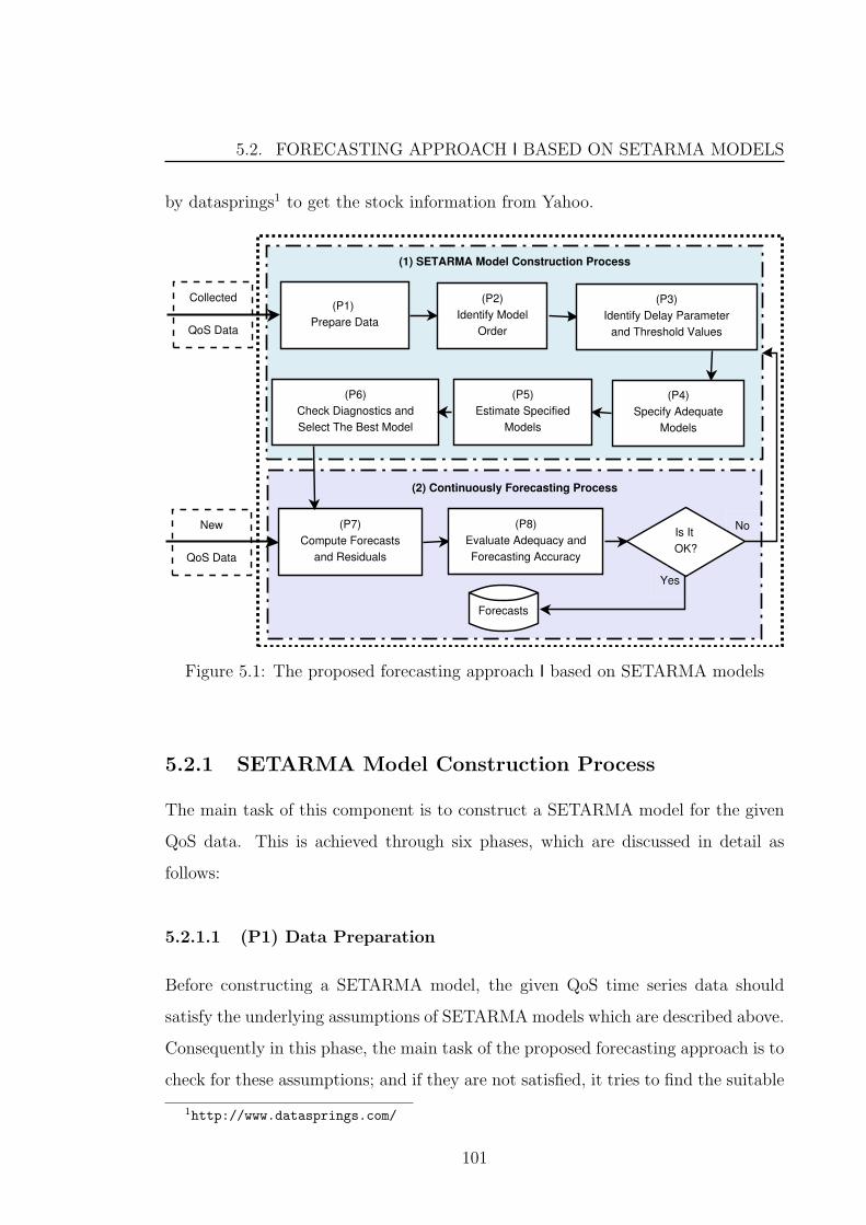
5.2. FORECASTING APPROACH I BASED ON SETARMA MODELS
by datasprings1 to get the stock information from Yahoo.
(1) SETARMA Model Construction Process
(2) Continuously Forecasting Process
Collected
QoS Data
New
QoS Data
(P8)
Evaluate Adequacy and
Forecasting Accuracy
(P7)
Compute Forecasts
and Residuals
Is It
OK?
No
Yes
(P1)
Prepare Data
(P2)
Identify Model
Order
(P4)
Specify Adequate
Models
(P5)
Estimate Specified
Models
(P6)
Check Diagnostics and
Select The Best Model
(P3)
Identify Delay Parameter
and Threshold Values
Forecasts
Figure 5.1: The proposed forecasting approach I based on SETARMA models
5.2.1 SETARMA Model Construction Process
The main task of this component is to construct a SETARMA model for the given
QoS data. This is achieved through six phases, which are discussed in detail as
follows:
5.2.1.1 (P1) Data Preparation
Before constructing a SETARMA model, the given QoS time series data should
satisfy the underlying assumptions of SETARMA models which are described above.
Consequently in this phase, the main task of the proposed forecasting approach is to
check for these assumptions; and if they are not satisfied, it tries to find the suitable
1http://www.datasprings.com/
101

CHAPTER 5. FORECASTING APPROACH FOR NONLINEARLYDEPENDENT QOS ATTRIBUTES
transformation to approximately fulfill the assumptions.
First, the forecasting approach checks for the serial dependency using the runs
test [77]. Then, it checks for the normality and stationarity using the Kolmogorov-
Smirnov (K-S) test [77] and the KPSS test [115], respectively. In case that the QoS
data is non-normally distributed, the approach uses the Box-Cox transformations
[32] to achieve the normality. On the other hand, it uses the differencing method to
produce a stationary QoS data.
Example . The proposed forecasting approach I prepares the WS1(RT) data as
follows:
Serial dependency: The forecasting approach applies the runs test to WS1(RT)
data and concludes that it is significantly serially dependent with a p-value < 0.05.
Normality: The forecasting approach applies the K-S test to WS1(RT) and con-
cludes that it is not normally distributed; however, the transformation parameter of
value “0.75” provides approximately normally distributed data which is referred as
WS1(TRT).
Stationarity: The forecasting approach uses the KPSS test to test whether the
time series WS1(TRT) is stationary, and finds that it is stationary where the p-
value equals to 0.238 (> 0.05). Therefore, the output of this phase is the dataset
WS1(TRT) that satisfies the assumptions and can be used in the next phases. /
5.2.1.2 (P2) Initial Model Order Identification
After preparing the QoS time series data, the forecasting approach identifies initial
values for the parameters p and q which determine an initial order for the SETARMA
model. The approach achieves this task based on evaluating the autocorrelation
function (ACF) and the partial autocorrelation function (PACF) of the given QoS
data [33].
Simply, the ACF is cross-correlations of the QoS time series data with itself at
102

5.2. FORECASTING APPROACH I BASED ON SETARMA MODELS
different time lags, and the autocorrelation at lag k is computed as follows [33]:
rk =
∑n−kt=1 (yt − y)(yt+k − y)∑n
t=1(yt − y)2, k = 0, 1, 2, . . . (5.8)
Regarding the PACF, generally the partial correlation between two variables is the
pure correlation of these two variables after eliminating the possible impact of all
other random variables that are correlated with them. To apply that to QoS time
series data, the PACF is computed as follows [33]:
φk =
∣∣∣∣∣∣∣∣∣∣∣∣
1 r1 . . . r1
r1 1 . . . r2
......
......
rk−1 rk−2 . . . rk
∣∣∣∣∣∣∣∣∣∣∣∣∣∣∣∣∣∣∣∣∣∣∣∣
1 r1 . . . rk−1
r1 1 . . . rk−2
......
......
rk−1 rk−2 . . . 1
∣∣∣∣∣∣∣∣∣∣∣∣
, k = 0, 1, 2, . . . (5.9)
where, rk is the autocorrelation coefficient at time lag k.
The ACF and PACF are used to identify the initial order of the SETARMA
model as follows. If the ACF curve decays and the PACF curve cuts off (after p
lags), a SETAR model (of order p) might be adequate to fit the processed data.
In contrast, if the ACF curve cuts off (after q lags) and the PACF curve decays, a
SETMA model (of order q) might be adequate. In addition, if both the ACF and
PACF curves cut off after q and p lags respectively, a SETARMA model (of order p
and q) might be adequate. Identifying the values of p and q is important for the next
phase P3 to specify the delay parameter and thresholds values which are required
as essential parameters for the SETARMA model.
Example . The forecasting approach computes the ACF and PACF of the pre-
pared data WS1(TRT), which are plotted in Figure 5.2. From this Figure it can
103

CHAPTER 5. FORECASTING APPROACH FOR NONLINEARLYDEPENDENT QOS ATTRIBUTES
be seen that the ACF decays and the PACF cuts off after 2 lags. Therefore, the
approach identifies the initial order of the SETARMA model as p = 2 and q = 0.
/
−0.2
0.0
0.2
0.4
0.6
0.8
Lag
AC
F
1 2 3 4 5 6 7 8 9 10 11 12 13 14 15 16 17 18 19 20
−0.2
0.0
0.2
0.4
0.6
0.8
Lag
PA
CF
1 2 3 4 5 6 7 8 9 10 11 12 13 14 15 16 17 18 19
Figure 5.2: ACF and PACF values of WS1(TRT)
5.2.1.3 (P3) Delay Parameter and Thresholds Identification
In this phase the forecasting approach needs to identify the values of delay parameter
and thresholds. To achieve this, the approach uses the Hansen test [90], which is
104

5.2. FORECASTING APPROACH I BASED ON SETARMA MODELS
introduced in Chapter 4. This test requires the parameter p and the delay parameter
dp as inputs. Although the value of the parameter p is already identified in P2 and
can be used by the test, the delay parameter dp is unknown and the approach needs
to identify. Therefore, the approach runs the Hansen test different times with all the
possible values of the delay parameter, which are any value less than the parameter
p, i.e. 0 < dp ≤ p. After that, based on the outputs of the Hansen tests the
proposed approach refines the delay parameter value as the value that corresponds
the largest statistic value of the significant Hansen test. Similarly, the thresholds
values are identified as the values that correspond the largest statistic value.
Example . Since the forecasting approach found in P2 that p = 2, it runs the
Hansen test two times with inputs (p = 2 and dp = 1) and (p = 2 and dp = 2), and
the output is depicted in Table 5.1. The forecasting approach concludes that the
delay parameter dp = 2 and the threshold value is 196.32. /
Delay Threshold Statistic
Value Estimate Value P-value
1 198.25 17.76 0.032
2 196.32 12.36 0.018
Table 5.1: Hansen test results for WS1(TRT)
5.2.1.4 (P4) Adequate Models Specification
After identifying the initial model order, delay parameter and threshold values,
the proposed forecasting approach specifies a combination of adequate SETARMA
models for the given QoS dataset. This combination is based on the dependency
structure of the given QoS dataset, in terms of the ACF and PACF, and under-
fitting and over-fitting methods. Let p and q be the initial model order and dp
be the delay parameter, then the combination of adequate SETARMA models that
can be specified are SETARMA(l, p± i, q ± j) for i = 1, 2 and j = 1, 2 with the
105

CHAPTER 5. FORECASTING APPROACH FOR NONLINEARLYDEPENDENT QOS ATTRIBUTES
conditions that (p− i) ≥ dp, (q − j) ≥ 0, (p+ i) ≤ 5 and (q + j) ≤ 5, assuming
that “5” is the highest order of the SETARMA models that can be fitted. This
assumption of the highest order is based on our experience, however, this value can
be easily changed and adapted to other values.
Example . As the identified initial order of the SETARMA model is p = 2
and q = 0 and the delay parameter is dp = 2, then based on the under-fitting and
over-fitting methods the forecasting approach identifies nine SETARMA models for
WS1(TRT) with the orders that are the combination of p = 2, 3, 4 and q = 0, 1, 2.
/
5.2.1.5 (P5) Models Estimation
In the models estimation phase, the forecasting approach estimates the parameters
of the specified adequate models in phase P4 to provide the best fit for the given QoS
time series data. The maximum likelihood estimation (MLE) [33] and conditional
least squares (CLS) [227] are the most commonly used methods to estimate the
SETARMA models’ parameters. However, Chan [47] showed that the CLS method
gives consistent estimators, which means that the estimates approach the true values
of the parameters with increasing sample size. Therefore, the CLS method is adopted
by the proposed forecasting approach I.
To briefly explain how the CLS method works, in the beginning, without loss
the generality of the SETARMA model (5.6), the SETARMA(2, p, q) model with the
delay parameter dp and the threshold value r (and assuming the homoscedasticity,
i.e. ε(j)t = εt for j = 1, . . . , l) can be rewritten as follows:
yt = ΩT1AtI[yt−dp ≤ r] + ΩT
2AtI[yt−dp>r] + εt (5.10)
where Ωj is the vector of SETARMA parameters of the jth regime, i.e. Ωj =
(φ(j)1 , . . . , φ
(j)p , θ
(j)1 , . . . , θ
(j)q )T for j = 1, 2; At is the lagged values of the given QoS
data represented in a data matrix, i.e. At = (1, yt−1, yt−2, . . . , yt−p)T ; and I[.] ∈
106

5.2. FORECASTING APPROACH I BASED ON SETARMA MODELS
0, 1 is the indicator function. Then, the estimate of Ω = (ΩT1 ,Ω
T2 )T can be easily
obtained by minimizing the conditional sum of squared errors, i.e. (yt−ΩTAr)T (yt−
ΩTAr), and written as follows:
Ω(r) = (AT(r)A(r))−1AT(r)yt (5.11)
where A(r) = (ATt I[yt−dp ≤ r], ATt I[yt−dp>r]) and from the used notation Ω(r) the
estimate of Ω is conditional upon the threshold value r. It is worth mentioning
that in the case of homoscedasticity, minimizing the residual sum of squares is
equivalent to maximizing the log-likelihood function. In other words, CLS estimates
are equivalent to those are given by maximum likelihood method.
Example . After identifying the adequate SETARMA models in P4, the fore-
casting approach uses the CLS method for each model to estimate the parameters.
The estimates of four of these identified SETARMA models are depicted in Table
5.2. /
5.2.1.6 (P6) Models Checking and the Best Model Selection
The forecasting approach checks the diagnostics of the SETARMA models to iden-
tify whether they are satisfied, and these diagnostics include the estimates signifi-
cance test, satisfaction of the stationarity and invertibility conditions and residuals
randomness. If one or more diagnostics are not satisfied, the current model is in-
adequate and it is necessary to be removed from the set of models specified in P4.
These diagnostics are discussed in detail as follows.
107

CHAPTER 5. FORECASTING APPROACH FOR NONLINEARLYDEPENDENT QOS ATTRIBUTES
Model Regime Parameter Estimate t-value P-value
I
LowSETAR(1) 0.757 6.215 0.000
SETAR(2) -0.177 -2.456 0.032
HighSETAR(1) 0.270 2.751 0.026
SETAR(2) 0.099 2.615 0.036
II
Low
SETAR(1) -0.715 -5.115 0.000
SETAR(2) -0.084 -2.661 0.028
SETMA(1) 0.433 2.456 0.038
High
SETAR(1) 0.669 2.436 0.047
SETAR(2) 0.074 2.499 0.041
SETMA(1) -0.325 -2.233 0.044
III
Low
SETAR(1) -0.552 -7.652 0.000
SETAR(2) -0.064 -3.121 0.028
SETAR(3) 0.051 2.856 0.033
High
SETAR(1) 0.268 2.897 0.025
SETAR(2) 0.187 2.775 0.041
SETAR(3) -0.075 -2.985 0.022
IV
Low
SETAR(1) -0.848 -6.235 0.000
SETAR(2) -0.076 -3.231 0.029
SETAR(3) 0.065 2.654 0.032
SETMA(1) 0.523 2.561 0.028
High
SETAR(1) 0.467 2.994 0.029
SETAR(2) 0.074 2.325 0.042
SETAR(3) -0.043 -2.661 0.026
SETMA(1) -0.456 -3.123 0.035
Table 5.2: Estimation of four identified SETARMA models
108

5.2. FORECASTING APPROACH I BASED ON SETARMA MODELS
Estimates Significance Test
Each estimate is tested to check whether it is statistically significant using the t-test,
which its statistic is computed as follows:
t− statistic =estimate value
standard error of estimate(5.12)
If all the estimates are significant, they are retained in the model; and otherwise,
the model requires a recalculation using only the significant estimates.
Stationarity and Invertibility Conditions Satisfaction
Stationarity and invertibility conditions for the general SETARMA model are still
under research, however, the forecasting approach I exploits the idea that at each
regime there is an ARMA model and thus applies the stationarity and invertibility
conditions of the general ARMA model. This means that the stationarity and
invertibility conditions for the SETARMA model can be initially checked as follows:
(1) Stationarity condition: The sum of the coefficients of the AR model at each
regime should be less than one, which means that∑p
i=1 φ(j)i < 1 for j = 1, 2, . . . , l;
and (2) Invertibility condition: The sum of the coefficients of the MA model at each
regime should be less than one, which means that∑q
i=1 θ(j)i < 1 for j = 1, 2, . . . , l.
Residuals Randomness
Residuals of the well constructed SETARMA model should be uncorrelated and do
not have any non-random pattern, which confirms that the model fits successfully
the given QoS data. Therefore, the forecasting approach analyzes the residuals and
performs a hypothesis test, i.e. the Box-Pierce test [34], to make a statistically
significant decision regarding the residuals randomness.
Once the specified SETARMA models have been estimated and checked, the
forecasting approach selects the best SETARMA model based on the Akaike’s infor-
109

CHAPTER 5. FORECASTING APPROACH FOR NONLINEARLYDEPENDENT QOS ATTRIBUTES
mation criterion (AIC) [1] where the best model is the one that has the minimum
AIC value. Hence AIC is an increasing function of the number of estimated param-
eters. This makes AIC biased to the overfitted models. Therefore, AIC is corrected
by penalizing the number of parameters as follows [103]:
AICc = AIC +2k(k + 1)
n− k − 1(5.13)
where k and n are the number of parameters in the estimated model and the number
of observations used to estimate the model, respectively. Following the recommen-
dations in [36], AICc is used by the proposed forecasting approach.
At the end, the selected best SETARMA model can be written as follows:
yt = µ(j) +
pj∑i=1
φ(j)i yt−i +
qj∑s=0
θ(j)s εt−s if rj−1 ≤ yt−dp < rj (5.14)
where φ(j)i ’s and θ
(j)s ’s for j = 1, 2, . . . , l are the conditional least squares estimates.
Example . The forecasting approach computes the t-test values and its p-values
for all the estimates of the nine SETARMA models, and it finds that the estimates of
four models are significant, and the other five models have insignificant estimates.
Therefore, the approach ignores these five models and focuses only on the four
models, which their t-values and p-values are depicted in Table 5.2. It is evident
from Table 5.2 that these models satisfy invertibility and stationarity conditions. To
analyze the residuals of the four models, the approach uses the Box-Pierce test [34]
and concludes that only the residuals of the last two models are uncorrelated. Now
based on the AICc value the forecasting approach selects the best model of those two
models, where the AICc values are: 1810.53 and 1790.34 respectively. Accordingly,
the fourth model, SETARMA(2, 3, 1), is the best model to forecast the future values
of WS1(RT). /
110

5.2. FORECASTING APPROACH I BASED ON SETARMA MODELS
5.2.2 Continuously Forecasting Process
The main task of this component is to use the selected best SETARMA model
and the new obtained QoS data to continuously forecast the future QoS values
and evaluate the adequacy and forecasting accuracy of the used SETARMA model,
which is achieved through two phases as discussed in detail as follows.
5.2.2.1 (P7) Computing Forecasts and Predictive Residuals
The proposed forecasting approach uses the selected best SETARMA model to fore-
cast the one-step-ahead future QoS values by moving from time “t” to “t + 1” as
follows:
yt+1 = µ(j) +
pj∑i=1
φ(j)i yt+1−i +
qj∑s=0
θ(j)s εt+1−s, (5.15)
and to compute the predictive residuals as:
εt = (yt − yt). (5.16)
Based on assuming that the new QoS data is continuously obtained, the approach
continuously computes the QoS forecasts and their predictive residuals.
Example . The forecasting approach uses the constructed SETARMA(2,3,1)
model with its parameters estimated in P5 to forecast the future values of WS1(RT),
and the one-step-ahead forecasts of the last 100 real response time observations and
their predictive residuals are computed and depicted in Figure 5.3. /
5.2.2.2 (P8) Evaluating Adequacy and Forecasting Accuracy
There is no guarantee that the stochastic behavior of the given QoS data will remain
constant over time. Therefore, the forecasting approach continuously evaluates the
adequacy and accuracy of the used SETARMA model. The approach evaluates the
adequacy by monitoring the predictive residuals. This is because the predictive
111

CHAPTER 5. FORECASTING APPROACH FOR NONLINEARLYDEPENDENT QOS ATTRIBUTES
0 20 40 60 80 100
10
00
11
00
12
00
13
00
Request Index
Re
sp
on
se
Tim
e (
ms)
Real
Predicted
0 20 40 60 80 100
−4
0−
20
02
04
06
0
Request Index
Pre
dic
tive
Re
sid
ua
ls
Figure 5.3: Real vs. predicted values of WS1(RT) and their predictive residuals
112

5.2. FORECASTING APPROACH I BASED ON SETARMA MODELS
residuals of adequate SETARMA model fluctuate around zero; and the changes in
the underlying QoS data will be immediately reflected in these predictive residuals
which will no longer fluctuate around zero and a positive or negative drift will
be introduced. To this end, the forecasting approach uses the CUSUM control
chart [174] as an efficient technique to monitor the predictive residuals and detect
their changes.
The CUSUM control chart monitors the predictive residuals by accumulating the
deviations that are above zero (the target value) with the one-sided upper CUSUM
statistic and deviations that are below zero with the one-sided lower CUSUM statis-
tic. The one-sided upper and lower CUSUM statistics are computed respectively as
follows:
C+t = max[0, εt − (µ0 +K) + C+
t−1]
C−t = min[0, εt − (µ0 +K) + C−t−1] (5.17)
where the starting values are C+0 = C−0 = 0, and µ0 = 0 is the target value. K
is called the reference value for the CUSUM control chart and often selected to be
0.5σe, where σe is the standard deviation of the predictive residuals [157]. Let H
be the decision interval, and it is usually chosen to be ±5σe [157]. Then, if the
predictive residuals start to systematically have positive or negative drift, one of
the CUSUM statistics will increase in magnitude till exceeds the decision interval
H and an out-of-control signal will be generated. This signal indicates that the
used SETARMA model is not adequate any more for the underlying QoS data and
new SETARMA model has to be constructed. (Regarding the choice of K and H,
Montgomery [157] introduces detailed discussion how these values can be chosen.)
In addition to monitoring the predictive residuals, the forecasting approach eval-
uates the forecasting accuracy by computing the mean absolute percentage error
(MAPE) metric (in Equation 3.7), which is discussed in Chapter 3. Therefore, the
MAPE value is used as a measure for the forecasting accuracy, where the smaller
value indicates the higher forecasting accuracy and vice versa.
In the case that the CUSUM control chart signals that the used SETARMA
113

CHAPTER 5. FORECASTING APPROACH FOR NONLINEARLYDEPENDENT QOS ATTRIBUTES
model is not adequate any more for the underlying QoS data or the forecasting
accuracy is very low based on the MAPE metric, the forecasting approach will re-
turn back to the first component to re-identify and re-construct other adequate SE-
TARMA model based on the new collected QoS data and the information obtained
from the predictive residuals analysis.
Example . The forecasting approach computes the CUSUM statistics for the
predictive residuals, as depicted in Figure 5.4. It is clear from this Figure that the
upper and lower CUSUM statistics do not exceed the decision interval, which indi-
cates that the used SETARMA model is still adequate for the underlying response
time data. In addition, the MAPE metric is computed and its value is 5.8%, which
is relatively small and indicates to be accepted forecasting accuracy. /
0 20 40 60 80 100
−300
−200
−100
010
020
030
0
Request Index
CU
SU
M S
tatis
tic
Upper Desdecision Interval
Lower Desdecision Interval
Upper CUSUM StatisticLower CUSUM Statistic
Figure 5.4: CUSUM statistics for the predictive residuals of WS1(RT)
114

5.3. SUMMARY
5.3 Summary
In this chapter, we first summarized the statistical background of the time series
models and discussed their main assumptions. We then introduced the proposed
forecasting approach I for nonlinearly dependent QoS attributes with a running
example of response time of a real-world Web service. This forecasting approach
is based on SETARMA time series models, and it will be able to effectively fit the
nonlinear dynamic behavior of QoS attributes and accurately forecast their future
values. However, the accuracy and performance of this forecasting approach need
to be evaluated and compared to those of the baseline ARIMA models which is
planned to be conducted in the evaluation chapter.
115

CHAPTER 5. FORECASTING APPROACH FOR NONLINEARLYDEPENDENT QOS ATTRIBUTES
116

Chapter 6
Forecasting Approaches for
Linearly Dependent QoS
Attributes with Volatility
Clustering
The objective of this chapter is to address the problem of forecasting linearly depen-
dent QoS attributes with volatility clustering. Based on our review of the time series
modeling literature, we have found that the generalized autoregressive conditional
heteroscedastic (GARCH) models [28] is a promising method to fit the QoS volatility
clustering and improve the ultimate QoS forecasting accuracy. Accordingly using
the GARCH models, we propose two approaches to model the linearly dependent
QoS attributes with volatility clustering:
• The first approach fits the given QoS data by ARIMA models, then com-
putes the squared residuals, which include the volatility clustering, and fits by
GARCH models.
• The second approach decomposes the given QoS data using wavelet analysis
into two simplified sub-series: the general trend, which is purified from the
117

CHAPTER 6. FORECASTING APPROACHES FOR LINEARLYDEPENDENT QOS ATTRIBUTES WITH VOLATILITY CLUSTERING
volatility clustering, and the noises component1, which includes the volatility
clustering. After that, it fits separately the general trend by ARIMA models
and the noises component by ARIMA and GARCH models. Similar approach
is proposed to forecast electricity price [223]
Consequently, in order to address the QoS volatility clustering and improving the
QoS forecasting accuracy we propose two different forecasting approaches. The
first forecasting approach, which is called forecasting approach II, is proposed based
on ARIMA and GARCH models. The main idea of this forecasting approach is
that it first constructs the best suitable ARIMA model for the given QoS data. It
then computes the squared residuals, which include the volatility clustering, and
constructs the best suitable GARCH model for the squared residuals. After that,
using the new obtained QoS data, the forecasting approach continuously updates
the constructed ARIMA-GARCH model, computes the QoS forecasts and evaluates
the adequacy and forecasting accuracy of the constructed ARIMA-GARCH model.
On the other hand, the second forecasting approach, which is called forecasting
approach III, is proposed based on the wavelet analysis, ARIMA and GARCH mod-
els. This forecasting approach first decomposes the complicated behavior of the given
QoS data using wavelet analysis into two simplified sub-series which are the gen-
eral trend and the noises component. Second, the forecasting approach constructs
an ARIMA model for the general trend sub-series and an ARIMA-GARCH model
for the noises component sub-series. Third, using the new obtained QoS data, the
forecasting approach continuously updates the constructed ARIMA and ARIMA-
GARCH models, computes the forecasts of the general trend and noises component
respectively, combines these forecasts to provide the original QoS forecasts and eval-
uates the adequacy and forecasting accuracy of the constructed models. Although
these two forecasting approaches II and III address the QoS volatility clustering, they
are not expected to be identical in terms of forecasting accuracy and performance.
1As a note on terminology, “noises component” is used as a specific term in this thesis whichrefers to a high frequency component of the given QoS time series data, and it does not refer tothe generic term of white noises.
118

6.1. BACKGROUND OF GARCH MODELS AND WAVELET ANALYSIS
In the rest of this chapter, we summarize the background of the GARCH models
and Wavelet Analysis. We then introduce the proposed forecasting approaches II
and III with a running example of response time of a real-world Web service.
6.1 Background of GARCH Models and Wavelet
Analysis
This section introduces the background of GARCH time series models and wavelet
analysis.
6.1.1 GARCH Models
The autoregressive conditional heteroscedastic (ARCH) models were introduced by
Engle [68] to model the high volatility by describing the dynamic changes in time-
varying variance as a deterministic function of past errors. These models have
become widely accepted for financial time series with volatility clustering and turned
out to be an important tool in the field of financial forecasting [102,124].
Engle formally defined the ARCH model for a conditional variance σ2t of the
dependent variable yt as:
σ2t = α0 + α1ε
2t−1 + · · ·+ αmε
2t−m, (6.1)
where, εt = yt −∑p
i=1 φiyt−i −∑q
i=1 θiεt−i, and m and αi for i = 0, ..., m are the
ARCH model order and coefficients respectively.
A generalization of ARCH model (GARCH) where additional dependencies are
permitted on lags of the conditional variance was introduced by Bollerslev [28].
Mainly, in GARCH model the conditional variance is more generalized than in
ARCH model and can be written as follows:
σ2t = α0 +
r∑i=1
αiε2t−i +
m∑j=0
βjσ2t−j. (6.2)
119

CHAPTER 6. FORECASTING APPROACHES FOR LINEARLYDEPENDENT QOS ATTRIBUTES WITH VOLATILITY CLUSTERING
with constraints,
α0>0, αi ≥ 0, βj ≥ 0, andr∑i=1
αi +m∑j=0
βj < 1. (6.3)
6.1.2 Wavelet Analysis
Wavelet analysis is a mathematical technique which breaks up a time series (signal)
into wavelets based on a specific wavelet transform [140]. More specifically, the
wavelet transform is a scaling function which converts a signal into a low and high
frequency components, which represent the general trend and noises component in
the original time series data respectively.
A time series yt can be decomposed into a series of wavelets as follows. First, the
scaling function ϕ(t) which called the father wavelet is defined as∫ +∞−∞ ϕ(t)dt = C,
where C is a constant, and the wavelet function ψ(t) which called the mother wavelet
is defined as∫ +∞−∞ ψ(t)dt = 0. These father and mother wavelets are orthogonal to
each other, i.e.∫ +∞−∞ ϕ(t)ψ(t)dt = 0, and their successive wavelets are obtained as
follows:
ϕk(t) = ϕ(t− k), k ∈ Z
ψk,j(t) = 22/jψ(2jt− k), (k, j) ∈ Z (6.4)
where k is a time factor and j is a scaling index. Then, the decomposition coefficients
of the wavelet transform of the original time series yt can be computed as follows:
wΦ(k) =
∫ +∞
−∞ytϕk(t)dt
wΨ(k, j) =
∫ +∞
−∞ytψk,j(t)dt (6.5)
Using the computed decomposition coefficients, the general trend (GTt) and noises
component (NCt) of the original time series data can be computed respectively as
120

6.2. FORECASTING APPROACH II BASED ON ARIMA AND GARCHMODELS
follows:
GTt =+∞∑
k=−∞
wΦ(k)ϕk(t)
NCt =+∞∑
k=−∞
+∞∑j=−∞
wΨ(k, j)ψk,j(t) (6.6)
6.2 Forecasting Approach II Based on ARIMA
and GARCH Models
The proposed forecasting approach II integrates ARIMA and GARCH models to
capture the QoS volatility clustering and accurately forecast their future values.
In brief summary, the forecasting approach first constructs the ARIMA model for
the given QoS data, and then computes the squared residuals, which include the
volatility clustering, and constructs the GARCH model. After that, using the new
obtained QoS data, the forecasting approach continuously updates the constructed
ARIMA-GARCH model, computes the QoS forecasts, and evaluates the adequacy
and forecasting accuracy of the constructed ARIMA-GARCH model. Consequently,
this forecasting approach consists of three components: ARIMA model construction
process, GARCH model construction process, and continuously forecasting process;
as explained in Figure 6.1. In the following the proposed forecasting approach II is
introduced in detail and explained by a running example of the response time dataset
(which is referred as WS2(RT)) of the web service ”GlobalWeather”1 which provides
the current weather along with additional information for major cities around the
world.
6.2.1 ARIMA Model Construction Process
This component uses the collected QoS data to construct the ARIMA model through
four phases as follows:
1http://www.webservicex.com/globalweather.asmx
121

CHAPTER 6. FORECASTING APPROACHES FOR LINEARLYDEPENDENT QOS ATTRIBUTES WITH VOLATILITY CLUSTERING
Collected
QoS Data
(P3)
Estimate Specified Models
(P4)
Check Diagnostics and
Select The Best Model
New
QoS Data
(P10)
Evaluate Adequacy and
Forecasting Accuracy
(P9)
Compute Forecasts
and Residuals
Is It
OK?
No
Yes
(3) Continuously Forecasting Process
(1) ARIMA Model Construction Process
(P1)
Check & Satisfy Assumptions
(P2)
Specify adequate Models
(P6)
Specify adequate Models
(P7)
Estimate Specified Models
(P8)
Check Diagnostics and
Select The Best Model
(2) GARCH Model Construction Process
Forecasts
(P5)
Compute Squared Residuals
Figure 6.1: The proposed forecasting approach II based on ARIMA and GARCHmodels
6.2.1.1 (P1) Data Preparation
Similarly to the forecasting approach I in Chapter 5, the forecasting approach II
uses some statistical tests to check for the underlying assumptions which include
the serial dependency, normality and stationarity before constructs the ARIMA
model. In addition, in the case that these assumptions are not satisfied, it tries
to find a suitable transformation to make the given QoS data approximately fulfils
them. In particular, the forecasting approach II checks for the serial dependency,
122

6.2. FORECASTING APPROACH II BASED ON ARIMA AND GARCHMODELS
normality and stationarity using the runs test [77], the Kolmogorov-Smirnov (K-
S) test [77], and the KPSS test [115], respectively. In addition, it uses the Box-
Cox transformations [32] and the differencing method to achieve the normality and
stationarize the given QoS data, respectively.
Example . The proposed forecasting approach II prepares the WS2(RT) data as
follows:
Serial dependency: The forecasting approach applies the runs test to WS2(RT)
data and concludes that it is significantly serially dependent with a p-value < 0.05.
Normality: The forecasting approach applies the K-S test to WS2(RT) and con-
cludes that it is not normally distributed; however, the transformation parameter of
value ”-0.156” provides approximately normally distributed data which is referred
as WS2(TRT).
Stationarity: The approach uses the KPSS test to test whether the time series
WS2(TRT) is stationary, and finds that it is not stationary where the p-value equals
to 0.039 (< 0.05). Using the first difference, the approach concludes that the dif-
ferenced data (referred as WS2(DTRT)) is stationary where the p-value equals to
0.493. /
6.2.1.2 (P2) Adequate Models Specification
After preparing the QoS data, the forecasting approach II identifies initial values
for the parameters p and q of the ARIMA model which determine the initial model
order. Similarly to the forecasting approach I in Chapter 5, the forecasting approach
II uses ACF and PACF to achieve this task as follows. If the ACF curve decays and
the PACF curve cuts off (after p lags), an AR model (of order p) might be adequate
to fit the processed data. In contrast, if the ACF curve cuts off (after q lags) and
the PACF curve decays, a MA model (of order q) might be adequate. In addition,
if both the ACF and PACF curves cut off after q and p lags respectively, an ARMA
model (of order p and q) might be adequate.
123

CHAPTER 6. FORECASTING APPROACHES FOR LINEARLYDEPENDENT QOS ATTRIBUTES WITH VOLATILITY CLUSTERING
After identifying the initial model order, the proposed forecasting approach II
specifies a combination of adequate ARIMA models for the given QoS dataset. Using
the same notion of SETARMA models specification introduced in Chapter 5, the
combination of ARIMA models is based on the dependency structure of the given
QoS dataset, in terms of the ACF and PACF, and under-fitting and over-fitting
methods. Let p and q be the initial model order and d be the differencing order
determined in P1, then the combination of adequate ARIMA models that can be
specified are ARIMA(p± i, d, q ± j) for i = 1, 2 and j = 1, 2 with the conditions
that (p− i) ≥ 0, (q − j) ≥ 0, (p− i) + (q − j) > 0, (p+ i) ≤ 5 and (q + j) ≤ 5,
assuming that “5” is the highest order of the ARIMA models that can be fitted.
This assumption of the highest order is based on our experience, however, this value
can be easily changed and adapted to other values.
Example . The forecasting approach computes the ACF and PACF of the pre-
pared data, WS2(DTRT), as plotted in Figure 6.2. From this Figure it can be seen
that the ACF cuts off after 3 lags and the PACF decays. Therefore, the forecasting
approach identifies the initial order of the ARIMA model as p = 0 and q = 3. It is
worth noting that d = 1 is already determined in P1. Based on the identified initial
ARIMA model order and the under-fitting and over-fitting methods the forecasting
approach identifies fifteen ARIMA models for WS2(DTRT) with the orders that are
the combination of p = 0, 1, 2 and q = 1, 2, 3, 4, 5. /
6.2.1.3 (P3) Models Estimation
In models estimation phase, the forecasting approach II estimates the parameters of
the identified combination of ARIMA models to provide the best fit to the given QoS
data. Similarly to SETARMA models, maximum likelihood estimation (MLE) [33]
and conditional least squares (CLS) [227] are the most commonly used methods to
estimate the ARIMA models’ parameters. However, the former one is generally the
preferred technique to fit ARIMA models, as it is faster and gives more accurate
124

6.2. FORECASTING APPROACH II BASED ON ARIMA AND GARCHMODELS
−0.4
−0.2
0.0
0.1
0.2
0.3
Lag
AC
F
1 2 3 4 5 6 7 8 9 10 11 12 13 14 15 16 17 18 19 20
−0.4
−0.3
−0
.2−
0.1
0.0
0.1
Lag
PA
CF
1 2 3 4 5 6 7 8 9 10 11 12 13 14 15 16 17 18 19
Figure 6.2: ACF and PACF values of WS2(DTRT)
estimates [33]. Therefore, the MLE method is adopted by the proposed forecasting
approach II.
To briefly explain how the MLE method works, suppose that yt for t = 1, 2, . . . , n
is a QoS time series modeled by the ARMA model (5.2), then the likelihood function,
l, is given by
l ∝ (σ2)−n2 exp
− 1
2σ2
n∑t=1
(yt −
p∑i=1
φiyt−i −q∑i=1
θiεt−i
)2 (6.7)
125

CHAPTER 6. FORECASTING APPROACHES FOR LINEARLYDEPENDENT QOS ATTRIBUTES WITH VOLATILITY CLUSTERING
where the values of the parameters φi’s and θi’s that maximize the likelihood function
(6.7) are called the maximum likelihood estimates.
Example . After identifying the adequate ARIMA models in P2, the forecasting
approach uses the MLE method for each model to estimate the parameters. The
estimates of eight of these identified ARIMA models are depicted in Table 6.1. /
6.2.1.4 (P4) Models Checking and the Best Model Selection
This phase has the same functionality as P6 of the forecasting approach I in Chapter
5, where it evaluates the diagnostics of the ARIMA models to identify whether they
are satisfied. If one or more diagnostics are not satisfied, the current ARIMA model
is inadequate and it is necessary to be removed from the set of models identified in
P2. These diagnostics include estimates significance, stationarity and invertibility
conditions, and residuals randomness.
After evaluating the diagnostics, the best ARIMA model is selected based on
the minimum AICc value. Then, the selected best ARIMA model can be written as
follows:
yt = µ+
p∑i=1
φiyt−i +
q∑i=1
θiεt−i (6.8)
where φi’s and θi’s are the maximum likelihood estimates.
Example . The forecasting approach computes the t-test values and its p-values
for all the estimates of the fifteen ARIMA models, and it finds that the estimates of
eight models are significant, and the other seven models have insignificant estimates.
Therefore, the approach ignores these seven models and focuses only on the eight
models, where their t-values and p-values are depicted in Table 6.1. It is evident
from Table 6.1 that these models satisfy invertibility and stationarity conditions.
The approach uses the Box-Pierce test [34] to analyze the residuals of the eight
models and concludes that the residuals of the first five models are correlated and
those of the last three models are uncorrelated. The forecasting approach selects
126

6.2. FORECASTING APPROACH II BASED ON ARIMA AND GARCHMODELS
Model Parameter Estimate t-value P-value
I AR(1) -0.485 -13.499 0.000
IIAR(1) 0.144 2.526 0.024
MA(1) -0.971 -25.526 0.000
IIIAR(1) -0.677 -17.813 0.000
AR(2) -0.292 -10.315 0.001
IV
AR(1) 0.157 3.389 0.023
AR(2) 0.128 2.766 0.034
MA(1) -0.985 -45.818 0.000
V
AR(1) -0.804 -16.652 0.001
AR(2) -0.113 -2.237 0.042
MA(1) -0.107 -2.972 0.028
MA(2) -0.813 -24.598 0.000
VI
AR(1) -0.738 -18.182 0.001
AR(2) -0.500 -10.742 0.002
AR(3) -0.159 -3.902 0.036
VII
AR(1) 0.163 3.998 0.035
AR(2) 0.131 3.211 0.038
AR(3) 0.130 3.108 0.039
MA(1) -0.956 -21.658 0.000
VIII
AR(1) -0.225 8.018 0.003
AR(2) 0.151 3.283 0.037
AR(3) 0.142 3.558 0.032
MA(1) -0.707 -2.499 0.042
MA(2) -0.183 -2.212 0.044
Table 6.1: Estimation of eight identified ARIMA models
127

CHAPTER 6. FORECASTING APPROACHES FOR LINEARLYDEPENDENT QOS ATTRIBUTES WITH VOLATILITY CLUSTERING
the best model of these three models based on the AICc value. The AICc values
for those three models are: 1503.73, 1403.58 and 1402.49 respectively. Accordingly,
the eighth model, ARIMA(3, 1, 2), is the best model to forecast the future values of
WS2(TRT). /
6.2.2 GARCH Model Construction Process
This component uses the residuals of the selected best ARIMA model to construct
the GARCH model, and this is achieved through four phases as follows:
6.2.2.1 (P5) Computing Squared Residuals
In this phase, the forecasting approach II uses the selected best ARIMA model to
compute the squared residuals that need to be used to construct the GARCH model.
Simply, this is achieved as follows:
ε2t =
(yt − µ−
p∑i=1
φiyt−i −q∑i=1
θiεt−i
)2
(6.9)
6.2.2.2 (P6 - P8) Adequate GARCH Model Construction
The forecasting approach II constructs the adequate GARCH model through phases
(P6 - P8). These phases are functionally the same as phases (P2 - P4). The main
difference is that in the diagnostics checking phase (P8) the approach does not check
for the stationarity and invertibility where the GARCH model does not require these
conditions, but needs to check for the GARCH model constraints in equation 6.3.
Example . The forecasting approach computes the squared residuals and their
ACF and PACF which are plotted in Figure 6.3. Since the ACF decays and
PACF cuts off after 2 lags, the forecasting approach identifies the initial order of
the GARCH model as r = 2 and m = 0.
Based on the identified initial GARCH model order and the under-fitting and
128

6.2. FORECASTING APPROACH II BASED ON ARIMA AND GARCHMODELS
over-fitting methods, the forecasting approach identifies twelve GARCH models with
the orders that are the combination of r = 1, 2, 3, 4 and m = 0, 1, 2. Then, the
approach uses the MLE method for each model to estimate the parameters and
computes the t-test values and its p-values for all the estimates; and it finds that
the estimates of only four models are significant, which their t-values and p-values
are depicted in Table 6.2. From this Table, it is evident that all the four models
satisfy the GARCH’s conditions in equation 6.3.
The forecasting approach uses the AICc value to select the best model, where
the AICc values for those four models are: 1361.09, 1341.58, 1362.29 and 1358.79
respectively. Consequently, the second model, GARCH(1, 1), is the best model that
can be used with ARIMA(3, 1, 2) to forecast the future values of WS2(TRT). /
Model Parameter Estimate t-value P-value
I ARCH(1) 0.153 2.112 0.035
IIARCH(1) 0.128 2.352 0.019
GARCH(1) 0.638 3.928 0.000
IIIARCH(1) 0.149 2.305 0.021
ARCH(2) 0.098 2.121 0.034
IV
ARCH(1) 0.124 1.975 0.048
ARCH(2) 0.003 1.972 0.049
GARCH(1) 0.635 2.673 0.008
Table 6.2: Estimation of four identified GARCH models
6.2.3 Continuously Forecasting Process
This component has the same functionality as the second component of the forecast-
ing approach I in Chapter 5, where it uses the constructed ARIMA-GARCH model
and the new obtained QoS data to continuously forecast the future QoS values and
computes the predictive residuals (through phase P9). Additionally through phase
129

CHAPTER 6. FORECASTING APPROACHES FOR LINEARLYDEPENDENT QOS ATTRIBUTES WITH VOLATILITY CLUSTERING
−0.2
0.0
0.1
0.2
0.3
0.4
Lag
AC
F
1 2 3 4 5 6 7 8 9 10 11 12 13 14 15 16 17 18 19 20
−0.1
0.0
0.1
0.2
0.3
0.4
Lag
PA
CF
1 2 3 4 5 6 7 8 9 10 11 12 13 14 15 16 17 18 19
Figure 6.3: ACF and PACF values of the squared residuals of WS2(TRT)
P10, it continuously evaluates the adequacy of the constructed ARIMA-GARCH
model for the underlying QoS data using the CUSUM control chart and the fore-
casting accuracy using the MAPE measure.
In the case that the CUSUM control chart signals that the constructed ARIMA-
GARCH model is not adequate any more for the underlying QoS data or the fore-
casting accuracy is very low based on the MAPE measure, the forecasting approach
will return back to P2 to re-identify and construct other adequate ARIMA-GARCH
model based on the new collected QoS data and the information obtained from the
130

6.3. FORECASTING APPROACH III BASED ON WAVELET ANALYSIS,ARIMA AND GARCH MODELS
predictive residuals analysis.
Example . The forecasting approach uses the constructed ARIMA(3,1,2)-
GARCH(1,1) model to forecast the future values of WS2(RT), and the one-step-
ahead forecasts of the last 100 observations and their predictive residuals are
depicted in Figure 6.4. In addition, the approach computes the CUSUM statistics
for the predictive residuals, as depicted in Figure 6.5. It is clear from this Figure
that the upper and lower CUSUM statistics do not exceed the decision interval,
which indicates that the used ARIMA(3,1,2)-GARCH(1,1) model is still adequate
for the underlying response time data. Moreover, the MAPE measure is computed
and its value is 5.9%, which is relatively small and indicates to be accepted
forecasting accuracy. /
6.3 Forecasting Approach III Based on Wavelet
Analysis, ARIMA and GARCH Models
The proposed forecasting approach III integrates wavelet analysis, ARIMA and
GARCH models to decompose the complicated behavior of the given QoS data
into two simplified sub-series to be able to capture the QoS volatility clustering and
provide accurate QoS forecasting.
In brief summary, the forecasting approach III first uses the wavelet analysis to
decompose the given QoS data into two sub-series; general trend sub-series, which
is purified form the volatility clustering, and noises sub-series, which includes the
volatility clustering. Second, the forecasting approach constructs an ARIMA model
for the general trend sub-series and an an ARIMA-GARCH model for the noises
sub-series. Third, using the new obtained QoS data, the forecasting approach con-
tinuously updates the constructed ARIMA and ARIMA-GARCH models, computes
the forecasts of the general trend and noises sub-series respectively, combines these
forecasts to provide the original QoS forecasts and evaluates the adequacy and fore-
casting accuracy of the constructed models.
131
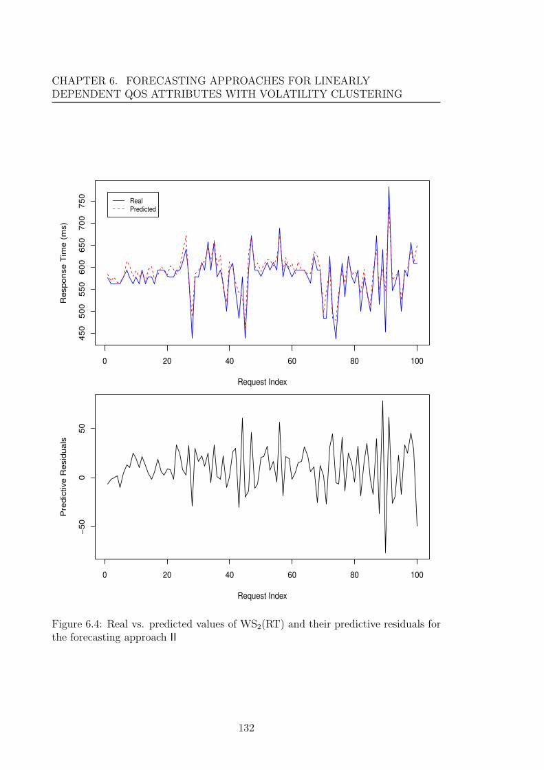
CHAPTER 6. FORECASTING APPROACHES FOR LINEARLYDEPENDENT QOS ATTRIBUTES WITH VOLATILITY CLUSTERING
0 20 40 60 80 100
45
05
00
55
06
00
65
07
00
75
0
Request Index
Re
sp
on
se
Tim
e (
ms)
Real
Predicted
0 20 40 60 80 100
−5
00
50
Request Index
Pre
dic
tive
Re
sid
ua
ls
Figure 6.4: Real vs. predicted values of WS2(RT) and their predictive residuals forthe forecasting approach II
132

6.3. FORECASTING APPROACH III BASED ON WAVELET ANALYSIS,ARIMA AND GARCH MODELS
0 20 40 60 80 100
−100
−50
050
100
150
Request Index
CU
SU
M S
tatis
tic
Upper Desdecision Interval
Lower Desdecision Interval
Upper CUSUM StatisticLower CUSUM Statistic
Figure 6.5: CUSUM statistics for the predictive residuals of WS2(RT) for the fore-casting approach II
Consequently, this approach consists of three components: Wavelet-based QoS
time series decomposition, ARIMA and ARIMA-GARCH models construction pro-
cess for the general trend and noises sub-series respectively, and continuously fore-
casting process; as explained in Figure 6.6. In the following the functionalities of
each component will be introduced with a running example of the same response
time dataset used in Section 6.2.
6.3.1 Wavelet-Based QoS Time Series Decomposition
This component uses wavelet analysis to decompose the given QoS data into the
general trend and noises component sub-series through two phases as follows.
133

CHAPTER 6. FORECASTING APPROACHES FOR LINEARLYDEPENDENT QOS ATTRIBUTES WITH VOLATILITY CLUSTERING
Collected
QoS Data
New
QoS Data
(P6)
Evaluate Adequacy and
Forecasting Accuracy
(P5)
Compute Forecasts
and Residuals
Is It
OK?
No
Yes
(3) Continuously Forecasting Process
(1) Wavelet-Based QoS Data Decomposition
(P1)
Select Wavelet Function
(P2)
Estimate Coefficients and
Construct Sub-Series
(P3)
Construct ARIMA Model for
General Trend Sub-Series
(2) ARIMA and ARIMA-GARCH Models Construction Process
Forecasts
(P4)
Construct ARIMA-GARCH
Model for Noises Sub-Series
Figure 6.6: The proposed forecasting approach III based on Wavelet analysis,ARIMA and GARCH models
6.3.1.1 (P1) Selecting Wavelet Function
In this phase, the forecasting approach III selects a wavelet function that can be
used to fit the QoS data under analysis. This wavelet function is expressed into
two functions, father ϕ(t) and mother ψ(t) functions. Several wavelet functions
are available such as Haar, Meyer and Daubechies wavelets [57, 140]. However, the
forecasting approach III adopts the Daubechies wavelet function as it is efficient and
the most commonly used in the practical applications [140].
Based on the Daubechies wavelet, the forecasting approach estimates the father
wavelet by defining its Fourier transform as follows:
ϕ(w) =1√2π
+∞∏j=−∞
m0(w/2j) (6.10)
134

6.3. FORECASTING APPROACH III BASED ON WAVELET ANALYSIS,ARIMA AND GARCH MODELS
where w is a Fourier variable and m0(w) is a periodic function defined as m0(w) =
eiw/2cos(w/2). Then, the father wavelet estimate is obtained as ϕ(t) = F−1(ϕ(w)),
where F−1 is the inverse Fourier transform. After estimating the father wavelet, the
mother wavelet is estimated as follows:
ψ(t) =+∞∑
k=−∞
bkϕ(2t− k) (6.11)
where bk is given by:
bk =
∫ +∞
−∞
√2ϕ(2t− k)ϕ(t)dt (6.12)
6.3.1.2 (P2) Estimating Decomposition Coefficients and Constructing
Sub-Series
After selecting the wavelet function and estimating the father and mother wavelets,
the forecasting approach fits the given QoS data on the estimated functions and
computes the decomposition coefficients as follows:
wΦ(k) =
∫ +∞
−∞ytϕk(t)dt
wΨ(k, j) =
∫ +∞
−∞ytψk,j(t)dt (6.13)
Then, the approach uses the computed decomposition coefficients and the estimated
father and mother functions to construct the general trend (GTt) and noises com-
ponent (NCt) as follows:
GTt =+∞∑
k=−∞
wΦ(k)ϕk(t)
NCt =+∞∑
k=−∞
+∞∑j=−∞
wΨ(k, j)ψk,j(t) (6.14)
135
CHAPTER 6. FORECASTING APPROACHES FOR LINEARLYDEPENDENT QOS ATTRIBUTES WITH VOLATILITY CLUSTERING
Example . The forecasting approach III uses the wavelet analysis to decompose
the WS2(RT) dataset into the general trend and noises component sub-series. The
WS2(RT) dataset and the constructed general trend and noises component sub-series
are depicted in Figure 6.7. /
6.3.2 ARIMA and ARIMA-GARCH Models Construction
Process
The main task of this component is to construct an ARIMA model for the general
trend (GTt) and an ARIMA-GARCH model for the noises component (NCt) through
two phases as follows.
6.3.2.1 (P3) Constructing ARIMA Model for the General Trend
In this phase, the forecasting approach III constructs an ARIMA model for the
general trend GTt. The forecasting approach achieves this task using the same
functionality of the first component of the forecasting approach II introduced in
Section 6.2.1.
Example . The forecasting approach III constructs an ARIMA model for the
general trend data constructed in P1 by first applying the K-S test and KPSS
test to check for the normality and stationarity respectively. The forecasting ap-
proach concludes that the general trend data is not normally distributed; however,
the transformation parameter of value ”1.8” provides approximately normally dis-
tributed data which is referred as GTt(TRT). In addition, it concludes that the
data is not stationary, however, the differenced data (referred as GTt(DTRT)) is
stationary using the first difference.
The approach computes the ACF and PACF of the prepared data, GTt(DTRT),
which are plotted in Figure 6.8. From this Figure it can be seen that the ACF
cuts off after 3 lags and the PACF decays. As a result, the initial identified order
of the ARIMA model is p = 0 and q = 3, in addition to that d = 1. Based on the
136

6.3. FORECASTING APPROACH III BASED ON WAVELET ANALYSIS,ARIMA AND GARCH MODELS
0 100 200 300 400 500
45
05
50
65
07
50
Request Index
Ori
gin
al R
T D
ata
(m
s)
0 100 200 300 400 500
50
05
50
60
06
50
Request Index
Ge
ne
ral Tre
nd
(m
s)
0 100 200 300 400 500
−1
00
05
01
00
Request Index
No
ise
s C
om
po
ne
nt
(ms)
Figure 6.7: The original WS2(RT) dataset and its constructed general trend andnoises component sub-series
137

CHAPTER 6. FORECASTING APPROACHES FOR LINEARLYDEPENDENT QOS ATTRIBUTES WITH VOLATILITY CLUSTERING
identified initial ARIMA model order and the under-fitting and over-fitting methods,
the approach identifies fifteen ARIMA models for GTt(DTRT) with the orders that
are the combination of p = 0, 1, 2 and q = 1, 2, 3, 4, 5.
The forecasting approach uses the MLE method for each model to estimate the
parameters and computes the t-test values and its p-values for all the estimates.
After that, the approach checks the diagnostics and uses the AICc value to select
the best ARIMA model that can be used to forecast the future values of GTt(TRT).
This model is ARIMA(3, 1, 2), which its estimates are presented in Table 6.3. /
−0.4
−0.2
0.0
0.2
0.4
Lag
AC
F
1 2 3 4 5 6 7 8 9 10 11 12 13 14 15 16 17 18 19 20
−0
.6−
0.4
−0.2
0.0
0.2
0.4
Lag
PA
CF
1 2 3 4 5 6 7 8 9 10 11 12 13 14 15 16 17 18 19
Figure 6.8: ACF and PACF values of GTt(DTRT)
138

6.3. FORECASTING APPROACH III BASED ON WAVELET ANALYSIS,ARIMA AND GARCH MODELS
Parameter Estimate t-value P-value
AR(1) 0.284 5.019 0.002
AR(2) -0.636 -11.311 0.001
MA(1) 0.636 3.469 0.021
MA(2) 0.257 6.125 0.001
Table 6.3: Estimates of the best ARIMA model for GTt(TRT)
6.3.2.2 (P4) Constructing ARIMA-GARCH Model for the Noises Com-
ponent
In this phase, the forecasting approach III constructs an ARIMA-GARCH model for
the noises component (NCt). The forecasting approach achieves this task using the
same functionality of the first and second components of the forecasting approach
II introduced in Sections 6.2.1 and 6.2.2.
Example . The forecasting approach III constructs an ARIMA-GARCH model
for the noises component data constructed in P1 by first applying the K-S test and
KPSS test to check for the normality and stationarity respectively. The forecasting
approach concludes that the noises component data (referred as NCt(RT)) is sta-
tionary and approximately normally distributed. The approach computes the ACF
and PACF of the NCt(RT) data as plotted in Figure 6.9, and finds that the ACF
decays and the PACF cuts off after 2 lags. As a result, the approach identifies the
initial order of the ARIMA model as p = 2 and q = 0, and identifies twelve ARIMA
models for NCt(RT) with the orders that are the combination of p = 1, 2, 3, 4 and
q = 0, 1, 2. After that, the approach estimates the twelve identified ARIMA models
using the MLE method, checks the diagnostics and uses the AICc value to select
the best ARIMA model that can be used to forecast the future values of NCt(RT).
This model is ARIMA(1, 0, 1), which its estimates are presented in Table 6.4.
To construct the GARCH model, the forecasting approach computes the squared
residuals and their ACF and PACF which are plotted in Figure 6.10. Since the ACF
139

CHAPTER 6. FORECASTING APPROACHES FOR LINEARLYDEPENDENT QOS ATTRIBUTES WITH VOLATILITY CLUSTERING
decays and the PACF cuts off after 2 lags, the approach identifies twelve GARCH
models with the orders that are the combination of r = 1, 2, 3, 4 and m = 0, 1, 2. The
approach estimates the twelve identified GARCH models using the MLE method,
checks the diagnostics and selects GARCH(1, 1) as the best GARCH model that can
be used with ARIMA(1, 0, 1) to forecast the future values of NCt(RT). The estimates
of GARCH(1, 1) are presented in Table 6.5. /
−0.6
−0.4
−0.2
0.0
0.2
0.4
Lag
AC
F
1 2 3 4 5 6 7 8 9 10 11 12 13 14 15 16 17 18 19 20
−0.6
−0.4
−0.2
0.0
0.2
0.4
Lag
PA
CF
1 2 3 4 5 6 7 8 9 10 11 12 13 14 15 16 17 18 19
Figure 6.9: ACF and PACF values of NCt(RT)
140

6.3. FORECASTING APPROACH III BASED ON WAVELET ANALYSIS,ARIMA AND GARCH MODELS
Parameter Estimate t-value P-value
AR(1) -0.530 -7.581 0.001
MA(1) -0.752 -45.484 0.000
Table 6.4: Estimates of the best ARIMA model for NCt(RT)
−0.2
−0.1
0.0
0.1
0.2
0.3
Lag
AC
F
1 2 3 4 5 6 7 8 9 10 11 12 13 14 15 16 17 18 19 20
−0
.3−
0.2
−0.1
0.0
0.1
0.2
0.3
Lag
PA
CF
1 2 3 4 5 6 7 8 9 10 11 12 13 14 15 16 17 18 19
Figure 6.10: ACF and PACF values of the squared residuals of NCt(RT)
141

CHAPTER 6. FORECASTING APPROACHES FOR LINEARLYDEPENDENT QOS ATTRIBUTES WITH VOLATILITY CLUSTERING
Parameter Estimate t-value P-value
ARCH(1) 0.563 3.415 0.001
GARCH(1) 0.385 3.984 0.000
Table 6.5: Estimates of the best GARCH model for the squared residuals of NCt(RT)
6.3.3 Continuously Forecasting Process
The main task of this component is to use the constructed ARIMA and ARIMA-
GARCH models and the new obtained QoS data to continuously forecast the future
QoS values and evaluate the adequacy and forecasting accuracy of the constructed
models, which is achieved through two phases discussed as follows.
6.3.3.1 (P5) Computing Forecasts and Predictive Residuals
The forecasting approach uses the new obtained QoS data and the constructed
ARIMA and ARIMA-GARCH models to continuously forecast the future values of
the general trend GTt and noises NCt sub-series respectively. Then, the approach
forecasts the future values of the given QoS data yt by combining the forecasts of
GTt and NCt sub-series. Simply, the one-step ahead forecast of yt is computed as
follows:
yt+1 = GT t+1 + NCt+1 (6.15)
where GT t+1 and NCt+1 are the one-step ahead forecasts of GTt and NCt sub-series
respectively, and the predictive residuals are computed as:
εt = (yt − yt). (6.16)
142
6.3. FORECASTING APPROACH III BASED ON WAVELET ANALYSIS,ARIMA AND GARCH MODELS
Example . The forecasting approach uses the constructed ARIMA(3, 1, 2) and
ARIMA(1, 0, 1)-GARCH(1, 1) models to forecast the future values of the GTt(RT)
and NCt(RT) datasets respectively. Then, by combing the forecasts of GTt(RT)
and NCt(RT) the approach forecasts the future values of the WS2(RT) dataset and
computes the predictive residuals. The one-step-ahead forecasts of the last 100
observations of the WS2(RT), GTt(RT) and NCt(RT) are depicted in Figure 6.11.
/
6.3.3.2 (P6) Evaluating Adequacy and Forecasting Accuracy
Similarly to the forecasting approaches I and II, the forecasting approach III con-
tinuously evaluates the adequacy of the constructed ARIMA and ARIMA-GARCH
models for the underlying QoS data using the CUSUM control chart and the fore-
casting accuracy using the MAPE measure.
In the case that the CUSUM control chart signals that the constructed ARIMA
and ARIMA-GARCH models are not adequate any more for the underlying QoS
data or the forecasting accuracy is very low based on the MAPE measure, the
forecasting approach will re-construct other adequate ARIMA and ARIMA-GARCH
models based on the new collected QoS data and the information obtained from the
predictive residuals analysis.
Example . The forecasting approach computes the upper and lower CUSUM
statistics for the predictive residuals, as depicted in Figure 6.12, which do not exceed
the decision interval and indicate that the used ARIMA(3, 1, 2) and ARIMA(1, 0, 1)-
GARCH(1, 1) models are still adequate for the underlying response time data. In
addition, the MAPE measure is computed and its value is 3.76%, which is relatively
small and indicates to be accepted forecasting accuracy. /
143

CHAPTER 6. FORECASTING APPROACHES FOR LINEARLYDEPENDENT QOS ATTRIBUTES WITH VOLATILITY CLUSTERING
0 20 40 60 80 100
45
05
50
65
07
50
Request Index
Ori
gin
al R
T D
ata
(m
s) Real
Predicted
0 20 40 60 80 100
50
05
50
60
06
50
Request Index
Ge
ne
ral Tre
nd
(m
s)
Real
Predicted
0 20 40 60 80 100
−1
00
05
01
00
Request Index
No
ise
s C
om
po
ne
nt
(ms) Real
Predicted
Figure 6.11: Real vs. predicted values of WS2(RT), GTt(RT) and NCt(RT)
144

6.4. SUMMARY
0 20 40 60 80 100
−50
050
Request Index
CU
SU
M S
tatis
tic
Upper Desdecision Interval
Lower Desdecision Interval
Upper CUSUM StatisticLower CUSUM Statistic
Figure 6.12: CUSUM statistics for the predictive residuals of WS2(RT) for theforecasting approach III
6.4 Summary
In this chapter, we first summarized the background of the GARCH models and
Wavelet Analysis. We then introduced the two proposed forecasting approaches
II and III with a running example of response time of a real-world Web service.
The forecasting approach II is based on ARIMA and GARCH models, while the
forecasting approach III is based on wavelet analysis, ARIMA and GARCH models.
These two forecasting approaches address the same problem of forecasting linearly
dependent QoS attributes with volatility clustering. However, the accuracy and
performance of these two forecasting approaches need to be evaluated in order to
conclude to what extent they are equivalent and identify their relative preferences.
145

CHAPTER 6. FORECASTING APPROACHES FOR LINEARLYDEPENDENT QOS ATTRIBUTES WITH VOLATILITY CLUSTERING
146

Chapter 7
Forecasting Approaches for
Nonlinearly dependent QoS
Attributes with Volatility
Clustering
The previous two chapters address separately the problems of nonlinearity and
volatility clustering of QoS attributes. Namely, Chapter 5 proposes the forecasting
approach I based on the SETARMA models to forecasting the nonlinearly dependent
QoS attributes with constant variance over time. In addition, Chapter 6 proposes
the forecasting approach II based on the ARIMA and GARCH models and the fore-
casting approach III based on the wavelet analysis, ARIMA and GARCH models to
forecasting the linearly dependent QoS attributes with volatility clustering. Conse-
quently, the current chapter builds on the proposed forecasting approaches in order
to address together the nonlinearity and volatility clustering of QoS attributes. This
chapter proposes two forecasting approaches to model the nonlinearly dependent
QoS attributes with volatility clustering and improve the forecasting accuracy.
The first forecasting approach, which is called forecasting approach IV, is pro-
posed based on SETARMA and GARCH models. On the other hand, the second
147

CHAPTER 7. FORECASTING APPROACHES FOR NONLINEARLYDEPENDENT QOS ATTRIBUTES WITH VOLATILITY CLUSTERING
forecasting approach, which is called forecasting approach V, is proposed based on
the wavelet analysis, SETARMA and GARCH models. These two forecasting ap-
proaches are introduced with a running example in the rest of this chapter.
7.1 Forecasting Approach IV Based on SE-
TARMA and GARCH Models
The proposed forecasting approach IV integrates SETARMA and GARCH models
to capture the nonlinearity and volatility clustering of QoS attributes and accurately
forecast future QoS values. In brief summary, the forecasting approach first con-
structs a SETARMA model for the given QoS data, computes the squared residuals
which include the volatility clustering, and constructs a GARCH model. After that,
the forecasting approach, by using the new obtained QoS data, continuously up-
dates the constructed SETARMA-GARCH model, computes the QoS forecasts and
evaluates the adequacy and forecasting accuracy of the constructed SETARMA-
GARCH model. Consequently, this forecasting approach consists of three compo-
nents: SETARMA model construction process, GARCH model construction process,
and continuously forecasting process; as explained in Figure 7.1. In the following the
proposed forecasting approach is introduced and explained by a running example of
the response time dataset (which is referred as WS3(RT)) of the web service ”Chi-
naStockWebService”1 which reports timely chinese stock market data, e.g. stock
name, price, ...etc.
7.1.1 SETARMA Model Construction Process
The main task of this component is to construct the SETARMA model for the
given QoS data. The forecasting approach IV achieves this task using the same
functionality of the first component of the forecasting approach I introduced in
Chapter 5 in Section 5.2.1. Briefly, the forecasting approach IV constructs the
1http://www.webxml.com.cn/WebServices/ChinaStockWebService.asmx
148

7.1. FORECASTING APPROACH IV BASED ON SETARMA AND GARCHMODELS
Collected
QoS Data
New
QoS Data
(P12)
Evaluate Adequacy and
Forecasting Accuracy
(P11)
Compute Forecasts
and Residuals
Is It
OK?
No
Yes
(3) Continuously Forecasting Process
(1) SETARMA Model Construction Process
(P8)
Specify adequate Models
(P9)
Estimate Specified Models
(P10)
Check Diagnostics and
Select The Best Model
(2) GARCH Model Construction Process
Forecasts
(P7)
Compute Squared Residuals
(P1)
Data Preparation
(P2)
Identify Model
Order
(P4)
Specify Adequate
Models
(P5)
Estimate Specified
Models
(P6)
Check Diagnostics and
Select The Best Model
(P3)
Identify Delay Parameter
and Threshold Values
Figure 7.1: The proposed forecasting approach IV based on SETARMA and GARCHmodels
SETARMA model for the given QoS data through six phases:
(P1) Data preparation: The forecasting approach prepares the QoS by checking
the serial dependency, normality and stationarity using the runs test [77],
Kolmogorov-Smirnov (K-S) test [77] and KPSS test [115], respectively. In
addition, the approach uses the Box-Cox transformations [32] and differencing
method to achieve the normality and stationarity, respectively.
(P2) Initial SETARMA model order identification: Using the autocorrelation func-
tion (ACF) and the partial autocorrelation function (PACF) [33] of the given
149
CHAPTER 7. FORECASTING APPROACHES FOR NONLINEARLYDEPENDENT QOS ATTRIBUTES WITH VOLATILITY CLUSTERING
QoS data, the forecasting approach identifies an initial order for the SE-
TARMA model.
(P3) Delay parameter and thresholds identification: Using the Hansen test [90], the
forecasting approach identifies the values of the delay parameter and thresholds
for the SETARMA model.
(P4) Adequate models specification: The forecasting approach specifies a combi-
nation of adequate SETARMA models for the given QoS data based on the
dependency structure, in terms of the ACF and PACF, and under-fitting and
over-fitting methods.
(P5) SETARMA models estimation: The forecasting approach estimates the param-
eters of the specified adequate models in P4 to provide the best fit for the given
QoS data using the conditional least squares (CLS) estimation method [227].
(P6) SETARMA models checking and the best model selection: The forecasting
approach checks the diagnostics of the SETARMA models to identify whether
they are satisfied, and these diagnostics include the estimates significance test,
satisfaction of the stationarity and invertibility conditions and residuals ran-
domness. If one or more diagnostics are not satisfied, the current SETARMA
model is inadequate and it is necessary to be removed from the set of models
specified in P4.
Example . The forecasting approach IV constructs a SETARMA model for the
WS3(RT) data by first applying the runs test, K-S test and KPSS test to check for the
serial dependency, normality and stationarity respectively. The forecasting approach
concludes that the WS3(RT) data is serially dependent and stationary, but not nor-
mally distributed; however, the transformation parameter of value ”0.322” provides
approximately normally distributed data which is referred as the WS3(TRT).
The approach computes the ACF and PACF of the prepared data, WS3(TRT),
which are plotted in Figure 7.2. From this Figure it can be seen that the ACF
150

7.1. FORECASTING APPROACH IV BASED ON SETARMA AND GARCHMODELS
decays and the PACF cuts off after 2 lags. As a result, the initial identified order
of the SETARMA model is p = 2 and q = 0. In addition, the approach runs the
Hansen test two times with inputs (p = 2 and dp = 1) and (p = 2 and dp = 2) and
based on the output identifies that the delay parameter dp = 1 and the threshold
value is 1530. Based on the identified initial SETARMA model order and the under-
fitting and over-fitting methods, the approach identifies twelve SETARMA models
for WS3(TRT) with the orders that are the combination of p = 1, 2, 3, 4 and q =
0, 1, 2.
The forecasting approach uses the CLS method for each model to estimate the
parameters and computes the t-test values and its p-values for all the estimates.
After that, the approach checks the diagnostics and uses the AICc value to select the
best SETARMA model that can be used to forecast the future values of WS3(TRT).
This model is SETARMA(2, 3, 0), which its estimates are presented in Table 7.1. /
Regime Parameter Estimate t-value P-value
Low
SETAR(1) 0.194 6.252 0.001
SETAR(2) 0.149 3.621 0.026
SETAR(3) 0.055 2.150 0.042
High
SETAR(1) 0.164 3.318 0.001
SETAR(2) 0.183 3.822 0.000
SETAR(3) 0.202 0.047 0.000
Table 7.1: Estimates of the best SETARMA model for WS3(TRT)
7.1.2 GARCH Model Construction Process
This component uses the residuals of the constructed SETARMA model to construct
the GARCH model. The forecasting approach IV achieves this task using the same
functionality of the second component of the forecasting approach II introduced in
151

CHAPTER 7. FORECASTING APPROACHES FOR NONLINEARLYDEPENDENT QOS ATTRIBUTES WITH VOLATILITY CLUSTERING
−0
.20
.00.2
0.4
0.6
Lag
AC
F
1 2 3 4 5 6 7 8 9 10 11 12 13 14 15 16 17 18 19 20
−0
.4−
0.2
0.0
0.2
0.4
0.6
Lag
PA
CF
1 2 3 4 5 6 7 8 9 10 11 12 13 14 15 16 17 18 19
Figure 7.2: ACF and PACF values of WS3(TRT)
Chapter 6 in Section 6.2.2. Briefly, the forecasting approach constructs the GARCH
model through four phases:
(P7) Computing squared residuals: The forecasting approach uses the constructed
SETARMA model to compute the squared residuals.
(P8) Adequate GARCH models specification: Using the ACF and the PACF of the
computed squared residuals, the forecasting approach identifies an adequate
GARCH models.
152

7.1. FORECASTING APPROACH IV BASED ON SETARMA AND GARCHMODELS
(P9) GARCH models estimation: The forecasting approach estimates the param-
eters of the specified adequate GARCH models in P8 using the maximum
likelihood estimation method [227].
(P10) GARCH models checking and the best model selection: The forecasting ap-
proach checks the diagnostics of the GARCH models which include the esti-
mates significance test, fulfilment of the GARCH model constraints (which are
presented in equation 6.3 in Chapter 6) and residuals randomness. If one or
more diagnostics are not satisfied, the current GARCH model is inadequate
and it is necessary to be removed from the set of models specified in P8.
Example . The forecasting approach computes the squared residuals and their
ACF and PACF which are plotted in Figure 7.3. Since the ACF decays and PACF
cuts off after 2 lags, the approach identifies the initial order of the GARCH model
as r = 2 and m = 0.
Based on the identified initial GARCH model order and the under-fitting and
over-fitting methods, the forecasting approach identifies twelve GARCH models with
the orders that are the combination of r = 1, 2, 3, 4 and m = 0, 1, 2. The approach
estimates the twelve identified GARCH models using the MLE method, checks the
diagnostics and selects GARCH(1, 1) as the best GARCH model that can be used
with SETARMA(2, 3, 0) to forecast the future values of WS3(TRT). The estimates
of GARCH(1, 1) are presented in Table 7.2. /
Parameter Estimate t-value P-value
ARCH(1) 0.155 2.983 0.003
GARCH(1) 0.804 15.638 0.000
Table 7.2: Estimates of the best GARCH model for the squared residuals ofWS3(TRT)
153

CHAPTER 7. FORECASTING APPROACHES FOR NONLINEARLYDEPENDENT QOS ATTRIBUTES WITH VOLATILITY CLUSTERING
−0.4
−0
.20.0
0.2
0.4
Lag
AC
F
1 2 3 4 5 6 7 8 9 10 11 12 13 14 15 16 17 18 19 20
−0.4
−0.2
0.0
0.2
0.4
Lag
PA
CF
1 2 3 4 5 6 7 8 9 10 11 12 13 14 15 16 17 18 19
Figure 7.3: ACF and PACF values of the squared residuals of WS3(TRT)
7.1.3 Continuously Forecasting Process
The forecasting approach IV uses the constructed SETARMA-GARCH model and
the new obtained QoS data to continuously forecast the future QoS values and eval-
uate the adequacy and forecasting accuracy of the constructed SETARMA-GARCH
model. The forecasting approach achieves this task using the same functionality
of the second component of the forecasting approach I introduced in Chapter 5 in
Section 5.2.2, which includes:
(P11) Computing forecasts and predictive residuals: The forecasting approach
154

7.2. FORECASTING APPROACH V BASED ON WAVELET ANALYSIS,SETARMA AND GARCH MODELS
uses the new obtained QoS data to continuously update the constructed
SETARMA-GARCH model and thus compute the predictive residuals.
(P12) Evaluating adequacy and forecasting accuracy of SETARMA-GARCH model:
The forecasting approach continuously evaluates the adequacy of the con-
structed SETARMA-GARCH model by using the CUSUM control chart [174]
to monitor the predictive residuals. In addition, the forecasting approach eval-
uates the forecasting accuracy by computing the mean absolute percentage
errors (MAPE) measure. In the case that the CUSUM control chart signals
that the used SETARMA-GARCH model is not adequate any more for the un-
derlying QoS data or the forecasting accuracy is very low based on the MAPE
measure, the forecasting approach will return back to the first component to
re-identify and construct other adequate SETARMA-GARCH model.
Example . The forecasting approach uses the constructed SETARMA(2,3,0)-
GARCH(1,1) model to forecast the future values of WS3(RT), and the one-step-
ahead forecasts of the last 100 observations and their predictive residuals are de-
picted in Figure 7.4. In addition, the CUSUM statistics for the predictive residuals
are computed and depicted in Figure 7.5. It is clear from this Figure that the
upper and lower CUSUM statistics do not exceed the decision interval, which indi-
cates that the used SETARMA(2,3,0)-GARCH(1,1) model is still adequate for the
underlying response time data. In addition, the MAPE measure is computed and
its value is 7.18%, which is relatively small and indicates to be accepted forecasting
accuracy. /
7.2 Forecasting Approach V Based on Wavelet
Analysis, SETARMA and GARCH Models
The proposed forecasting approach V integrates wavelet analysis, SETARMA and
GARCH models to decompose the complicated behavior of the given QoS data
155

CHAPTER 7. FORECASTING APPROACHES FOR NONLINEARLYDEPENDENT QOS ATTRIBUTES WITH VOLATILITY CLUSTERING
0 20 40 60 80 100
150
020
00
2500
Request Index
Resp
onse T
ime (
ms)
Real
Predicted
0 20 40 60 80 100
−20
00
100
200
Request Index
Pre
dic
tive R
esid
uals
Figure 7.4: Real vs. predicted values of WS3(RT) and their predictive residuals forthe forecasting approach IV
156

7.2. FORECASTING APPROACH V BASED ON WAVELET ANALYSIS,SETARMA AND GARCH MODELS
0 20 40 60 80 100
−400
−200
020
040
0
Request Index
CU
SU
M S
tatis
tic
Upper Desdecision Interval
Lower Desdecision Interval
Upper CUSUM StatisticLower CUSUM Statistic
Figure 7.5: CUSUM statistics for the predictive residuals of WS3(RT) for the fore-casting approach IV
into two simplified sub-series to be able to capture the nonlinearity and volatility
clustering of QoS attributes and provide accurate QoS forecasting.
In brief summary, the forecasting approach V first decomposes the complicated
behavior of the given QoS data using wavelet analysis into two simplified sub-series:
the general trend, which is purified from the volatility clustering, and the noises
component, which includes the volatility clustering. Second, the forecasting ap-
proach constructs a SETARMA model for the general trend and a SETARMA-
GARCH model for the noises component. Third, the forecasting approach, by us-
ing the new obtained QoS data, continuously updates the constructed SETARMA
and SETARMA-GARCH models, computes the forecasts of the general trend and
157

CHAPTER 7. FORECASTING APPROACHES FOR NONLINEARLYDEPENDENT QOS ATTRIBUTES WITH VOLATILITY CLUSTERING
noises component respectively, combines these forecasts to provide the original QoS
forecasts, and evaluates the adequacy and forecasting accuracy of the constructed
model.
Consequently, this forecasting approach consists of three components: Wavelet-
based QoS time series decomposition, SETARMA and SETARMA-GARCH models
construction process for the general trend and noises sub-series respectively, and
continuously forecasting process; as explained in Figure 7.6. In the following the
proposed forecasting approach is introduced and explained by a running example of
the same response time dataset used in Section 7.1.
Collected
QoS Data
New
QoS Data
(P6)
Evaluate Adequacy and
Forecasting Accuracy
(P5)
Compute Forecasts
and Residuals
Is It
OK?
No
Yes
(3) Continuously Forecasting Process
(1) Wavelet-Based QoS Data Decomposition
(P1)
Select Wavelet Function
(P2)
Estimate Coefficients and
Construct Sub-Series
(P3)
Construct SETARMA Model for
General Trend Sub-Series
(2) SETARMA and SETARMA-GARCH Models
Construction Process
Forecasts
(P4)
Construct SETARMA-GARCH
Model for Noises Sub-Series
Figure 7.6: The proposed forecasting approach V based on Wavelet analysis, SE-TARMA and GARCH models
158
7.2. FORECASTING APPROACH V BASED ON WAVELET ANALYSIS,SETARMA AND GARCH MODELS
7.2.1 Wavelet-Based QoS Time Series Decomposition
This component uses wavelet analysis to decompose the given QoS data into the gen-
eral trend GTt and noises component NCt sub-series by using the same functionality
of the first component of the forecasting approach III introduced in Chapter 6 in Sec-
tion 6.3.1. Briefly, the forecasting approach first adopts the Daubechies wavelet [57]
and estimates its father ϕ(t) and mother ψ(t) functions. Then, the approach com-
putes the decomposition coefficients and constructs the general trend GTt and noises
component NCt sub-series.
Example . The forecasting approach V uses the wavelet analysis to decompose
the WS3(RT) dataset into the general trend and noises component sub-series. The
WS3(RT) dataset and the constructed general trend and noises component sub-series
are depicted in Figure 7.7. /
7.2.2 SETARMA and SETARMA-GARCH Models Con-
struction Process
The main task of this component is to construct a SETARMA model for the general
trend GTt and a SETARMA-GARCH model for the noises component NCt through
two phases as follows.
7.2.2.1 (P3) Constructing SETARMA Model for the General Trend
In this phase, the forecasting approach V constructs a SETARMA model for the gen-
eral trend GTt using the same functionality of the first component of the forecasting
approach IV introduced in Section 7.1.1.
Example . The forecasting approach V constructs a SETARMA model for the
general trend data GTt(RT), and concludes that the SETARMA(2, 2, 0) is the best
SETARMA model that can be used to forecast the future values of GTt(RT). The
estimates of SETARMA(2, 2, 0) are presented in Table 7.3 /
159

CHAPTER 7. FORECASTING APPROACHES FOR NONLINEARLYDEPENDENT QOS ATTRIBUTES WITH VOLATILITY CLUSTERING
0 100 200 300 400 500
10
00
20
00
30
00
Request Index
Ori
gin
al R
T D
ata
(m
s)
0 100 200 300 400 500
15
00
20
00
25
00
Request Index
Ge
ne
ral Tre
nd
(m
s)
0 100 200 300 400 500
−5
00
05
00
Request Index
No
ise
s C
om
po
ne
nt
(ms)
Figure 7.7: The original WS3(RT) dataset and its constructed general trend andnoises component sub-series
160

7.2. FORECASTING APPROACH V BASED ON WAVELET ANALYSIS,SETARMA AND GARCH MODELS
Regime Parameter Estimate t-value P-value
LowSETAR(1) 0.415 1.982 0.043
SETAR(2) 0.176 2.240 0.025
HighSETAR(1) 0.172 3.344 0.001
SETAR(2) 0.232 4.919 0.000
Table 7.3: Estimates of the best SETARMA model for GTt(RT)
7.2.2.2 (P4) Constructing SETARMA-GARCH Model for the Noises
Component
In this phase, the forecasting approach V constructs a SETARMA-GARCH model
for the noises component NCt using the same functionality of the first and second
components of the forecasting approach IV introduced in Sections 7.1.1 and 7.1.2.
Example . The forecasting approach V constructs a SETARMA-GARCH model
for the noises component data NCt(RT), and concludes that the SETARMA(2, 2, 0)-
GARCH(1, 1) is the best model that can be used to forecast the future values of
NCt(RT). The estimates of SETARMA(2, 2, 0)-GARCH(1, 1) are presented in Tables
7.4 and 7.5. /
Regime Parameter Estimate t-value P-value
LowSETAR(1) -0.394 -23.588 0.000
SETAR(2) -0.249 -7.426 0.000
HighSETAR(1) -0.635 -31.298 0.000
SETAR(2) -0.346 -20.434 0.000
Table 7.4: Estimates of the best SETARMA model for NCt(RT)
7.2.3 Continuously Forecasting Process
The forecasting approach V uses the constructed SETARMA and SETARMA-
GARCH models and the new obtained QoS data to continuously forecast the future
161
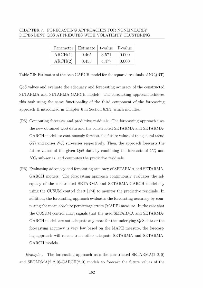
CHAPTER 7. FORECASTING APPROACHES FOR NONLINEARLYDEPENDENT QOS ATTRIBUTES WITH VOLATILITY CLUSTERING
Parameter Estimate t-value P-value
ARCH(1) 0.465 3.571 0.000
ARCH(2) 0.455 4.477 0.000
Table 7.5: Estimates of the best GARCH model for the squared residuals of NCt(RT)
QoS values and evaluate the adequacy and forecasting accuracy of the constructed
SETARMA and SETARMA-GARCH models. The forecasting approach achieves
this task using the same functionality of the third component of the forecasting
approach II introduced in Chapter 6 in Section 6.3.3, which includes:
(P5) Computing forecasts and predictive residuals: The forecasting approach uses
the new obtained QoS data and the constructed SETARMA and SETARMA-
GARCH models to continuously forecast the future values of the general trend
GTt and noises NCt sub-series respectively. Then, the approach forecasts the
future values of the given QoS data by combining the forecasts of GTt and
NCt sub-series, and computes the predictive residuals.
(P6) Evaluating adequacy and forecasting accuracy of SETARMA and SETARMA-
GARCH models: The forecasting approach continuously evaluates the ad-
equacy of the constructed SETARMA and SETARMA-GARCH models by
using the CUSUM control chart [174] to monitor the predictive residuals. In
addition, the forecasting approach evaluates the forecasting accuracy by com-
puting the mean absolute percentage errors (MAPE) measure. In the case that
the CUSUM control chart signals that the used SETARMA and SETARMA-
GARCH models are not adequate any more for the underlying QoS data or the
forecasting accuracy is very low based on the MAPE measure, the forecast-
ing approach will re-construct other adequate SETARMA and SETARMA-
GARCH models.
Example . The forecasting approach uses the constructed SETARMA(2, 2, 0)
and SETARMA(2, 2, 0)-GARCH(2, 0) models to forecast the future values of the
162

7.2. FORECASTING APPROACH V BASED ON WAVELET ANALYSIS,SETARMA AND GARCH MODELS
0 20 40 60 80 100
1500
2000
2500
Request Index
Ori
gin
al R
T D
ata
(m
s)
Real
Predicted
0 20 40 60 80 100
1200
1600
2000
Request Index
Genera
l Tre
nd (
ms)
Real
Predicted
0 20 40 60 80 100
−400
0200
Request Index
Nois
es C
om
ponent (m
s) Real
Predicted
Figure 7.8: Real vs. predicted values of WS3(RT) and their predictive residuals forthe forecasting approach V
163

CHAPTER 7. FORECASTING APPROACHES FOR NONLINEARLYDEPENDENT QOS ATTRIBUTES WITH VOLATILITY CLUSTERING
GTt(RT) and NCt(RT) datasets respectively. Then, by combing the forecasts of
GTt(RT) and NCt(RT) the approach forecasts the future values of the WS3(RT)
dataset and computes the predictive residuals. The one-step-ahead forecasts of the
last 100 observations of the WS3(RT), GTt(RT) and NCt(RT) are depicted in Figure
7.8. In addition, the CUSUM statistics for the predictive residuals are computed
and depicted in Figure 7.9. It is clear from this Figure that the upper and lower
CUSUM statistics do not exceed the decision interval, which indicates that the used
models is still adequate for the underlying response time data. In addition, the
MAPE measure is computed and its value is 5.52%, which is relatively small and
indicates to accepted forecasting accuracy. /
0 20 40 60 80 100
−300
−200
−100
010
020
030
0
Request Index
CU
SU
M S
tatis
tic
Upper Desdecision Interval
Lower Desdecision Interval
Upper CUSUM StatisticLower CUSUM Statistic
Figure 7.9: CUSUM statistics for the predictive residuals of WS3(RT) for the fore-casting approach V
164

7.3. SUMMARY
7.3 Summary
In this chapter, we introduced the two proposed forecasting approaches IV and V
with a running example of response time of a real-world Web service. These two
forecasting approaches build on the proposed forecasting approaches in previous
chapters in order to address together the nonlinearity and volatility clustering of
QoS attributes and improve the forecasting accuracy. The forecasting approach IV
is based on the SETARMA and GARCH models, while the forecasting approach V is
based on the wavelet analysis, SETARMA and GARCH models. In the next chapter,
we evaluate the accuracy and performance of the proposed forecasting approaches
and accordingly compare each one to another as well as to the baseline ARIMA
models.
165

CHAPTER 7. FORECASTING APPROACHES FOR NONLINEARLYDEPENDENT QOS ATTRIBUTES WITH VOLATILITY CLUSTERING
166

Chapter 8
Experimental Evaluation
In this chapter we evaluate accuracy and performance aspects of the proposed fore-
casting approaches and compare them to those of the baseline ARIMA models. In
general, we achieve this evaluation as follows. First, we apply the proposed fore-
casting approaches and the baseline ARIMA models to the collected QoS datasets,
which are discussed in Chapter 4. We then compute and investigate relative predic-
tive errors and the MAPE metric as a measure for the accuracy of forecasting QoS
values, contingency table-based metrics as a measure for the accuracy of forecasting
QoS violations, and time required to construct and use the time series model as a
measure for the performance.
In the rest of this chapter, we first introduce the experiment setup. We then
investigate and discuss in detail the results. Finally, we present general discussion
based on the results and highlight threats to validity of the work.
8.1 Experiment Setup
As mentioned in Chapter 3, the accuracy and performance aspects of the proposed
forecasting approaches need to be evaluated. In particular, the accuracy of the pro-
posed forecasting approaches is classified into two types; the accuracy of forecasting
QoS values and the accuracy of forecasting QoS violations. In addition, the perfor-
167

CHAPTER 8. EXPERIMENTAL EVALUATION
mance is measured by the time required by the forecasting approaches to construct
and use the time series model. Accordingly, we identify the following main evalua-
tion questions.
EQ1: Are the proposed forecasting approaches able to capture the dynamic behav-
ior of QoS attributes and improve the forecasting accuracy compared to the baseline
ARIMA model?
EQ2: To what extent the proposed forecasting approaches are able to correctly
forecast QoS violations compared to the baseline ARIMA model?
EQ3: What time is required for the forecasting approaches to automatically con-
struct and use the forecasting model?
In order to answer EQ1, the proposed forecasting approaches and baseline
ARIMA models are applied to the real-world response time and time between fail-
ures datasets that we have collected as discussed in detail in Chapter 4. Specifically,
the datasets are classified according to the main characteristics of the QoS attributes
into three groups which are:
• Nonlinearly dependent with constant variance over time.
• Linearly dependent with volatility clustering.
• Nonlinearly dependent with volatility clustering.
Where each group includes 100 datasets of response time and 40 datasets of time
between failures. In order to construct the forecasting model, in the case of response
time the forecasting approaches and the ARIMA model use the first 500 observations
in the dataset as a training set. However, in the case of time between failures the
number of observations considered as a training set depends on the size of the
dataset, especially most of the size of time between failures datasets is less than
200 observations. The constructed forecasting models by the forecasting approaches
and the ARIMA model are used to compute the predictions, and for each dataset
prediction the relative prediction errors are computed as follows:
errort = |yt − ytyt| × 100, for t = 1, 2, . . . , n (8.1)
168

8.1. EXPERIMENT SETUP
where yt and yt are the real and predicted values, respectively. These errors are
analyzed using boxplots and descriptive statistics. In addition, the MAPE metric
(in Equation 3.7), which is discussed in Chapter 3, is computed. The non-parametric
Mann-Whitney test [77] is used to test whether the proposed forecasting approaches
significantly outperform the baseline ARIMA model in terms of forecasting accuracy.
To quantify the difference in MAPE values, the effect size [51] is computed as follows:
effect size =MAPEARIMA −MAPEProposed√
(σ2ARIMA + σ2
Proposed)/2(8.2)
where MAPEARIMA and σ2ARIMA refer to the MAPE value and the variance of rel-
ative prediction errors produced by the baseline ARIMA models, respectively, and
MAPEProposed and σ2Proposed refer to the MAPE value and the variance of relative
prediction errors produced by one of the proposed forecasting approaches, respec-
tively. Moreover, the relative forecasting accuracy improvement (RAI) is measured
using a metric which is defined as follows:
RAI =MAPEARIMA −MAPEProposed
MAPEARIMA
× 100 (8.3)
In order to address EQ2, requirements of the response time and time between
failures of each Web service are specified, and then the proposed forecasting ap-
proaches and the baseline ARIMA model are applied (using the same setting in
EQ1) to forecast the violations of these requirements. After that, contingency
table-based metrics, especially negative predictive value (NPV), specificity value
(SV), F-measure value (FMV), and accuracy value (AV) metrics discussed in Chap-
ter 3, are computed for each Web service in order to assess the forecasting accuracy
of requirement violations considering different cases. In addition, the Mann-Whitney
test is used to test whether the proposed forecasting approaches significantly outper-
form the baseline ARIMA model in terms of these contingency table-based metrics,
along with computing the effect size values.
EQ3 is simply addressed by computing the time required for the forecasting
169

CHAPTER 8. EXPERIMENTAL EVALUATION
approaches and the baseline ARIMA models to automatically construct and use the
forecasting model. As a platform for our experiments, we used a Windows-based
PC equipped with a 3.00 GHz dual-core processor and 4GB main memory.
8.2 Results
In this section, the experiments results are introduced and discussed for each eval-
uation question, and separately for the response time and time between failures.
8.2.1 EQ1. Improving Forecasting Accuracy of QoS Values
Compared to Baseline ARIMA Model
8.2.1.1 Nonlinearly Dependent QoS Attributes
The boxplots of the relative prediction errors produced by the proposed forecasting
approach I and the baseline ARIMA model for nonlinearly dependent response time
and time between failures are depicted in Figures 8.1 and 8.2, respectively. In
addition, the MAPE values of the forecasting approach I and the baseline ARIMA
model are reported separately for each dataset in Table 8.1. (It is worth mentioning
that the detailed description of the Web services labeled in the Tables is introduced
in Appendix A.)
The boxplots in Figures 8.1 and 8.2 indicate that the forecasting approach I can
provide more accurate forecasts than the ARIMA model, where the prediction errors
exhibited by this approach are significantly lower than those of ARIMA models.
This result is confirmed by the Mann-Whitney test where the p-values < 0.05.
More precisely, the forecasting approach I produces MAPE values are on average
4.75 and 18.99 compared to 6.08 and 24.85 produced by the ARIMA model with
effect size values are 0.26 and 0.35 for the response time and time between failures,
respectively. This highlights that the forecasting approach I achieves forecasting
accuracy improvement of about 21.4% in the case of the response time and bout
23% in the case of the time between failures. It is worth initially noting that the
170

8.2. RESULTS
Re
lativ
e P
red
ictio
n E
rro
r (%
)
05
10
15
20
25
ARIMA Approach I
Figure 8.1: Boxplots of relative prediction errors for nonlinearly dependent responsetime
Re
lativ
e P
red
ictio
n E
rro
r (%
)
02
04
06
08
0
ARIMA Approach I
Figure 8.2: Boxplots of relative prediction errors for nonlinearly dependent timebetween failures
171

CHAPTER 8. EXPERIMENTAL EVALUATION
accuracy of the forecasting approach I and the baseline ARIMA model in the case of
the response time is better than that in the case of the time between failures. This
point will be discussed in detail at the end of this chapter.
These boxplots show another observation that the variation of prediction errors
exhibited by the proposed forecasting approach I is significantly lower than that of
the ARIMA model. Where, in the case of the response time 50% of the prediction
errors are within (1.71, 7.11) with an interquartile range (IQR) = 5.4 for the fore-
casting approach I, and within (1.91, 9.61) with an IQR = 7.1 for the ARIMA model.
Similarly, in the case of the time between failures 50% of the prediction errors are
within (12.66, 21.21) with an IQR = 14.3 for the forecasting approach I, and within
(19.12, 27.28) with an IQR = 15.3 for the ARIMA model. This indicates that the
forecasting accuracy of the approach I is more stable across different QoS datasets
than that of the ARIMA model.
For each Web service in Table 8.1, the results show that the forecasting approach I
outperforms the ARIMA model in all the cases of the response time and time between
failures. This result is confirmed by the Mann-Whitney test where the p-values <
0.05. The lowest and highest accuracy improvement of the forecasting approach I
compared to the ARIMA model for the response time are in the cases of WS1 with
the RAI is about 11.7% and WS2 with the RAI is about 30.3% respectively, and for
the time between failures are in the cases of WS14 with the RAI is about 15.8% and
WS13 with the RAI is about 31% respectively.
I The forecasting approach I outperforms the ARIMA model in forecasting QoS
values with accuracy improvement of about 21.4% and 23% for the response
time and time between failures, respectively.
172

8.2. RESULTS
ARIMA Approach I
WSid MAPE MAPE RAI
WS1 7.18 6.34 11.72
WS2 8.34 5.81 30.32
WS3 5.41 4.33 19.86
WS4 3.55 3.13 11.99
WS5 4.92 3.68 25.26
WS6 5.37 3.86 28.07
WS7 5.54 4.88 11.91
WS8 6.64 4.90 26.30
WS9 11.52 8.79 23.67
WS10 2.34 1.76 24.80
Average 6.08 4.75 21.39
(a) Results for response time
ARIMA Approach I
WSid MAPE MAPE RAI
WS2 25.74 19.86 22.84
WS5 27.91 21.20 24.04
WS11 26.29 19.65 25.25
WS12 17.40 13.83 20.50
WS13 30.55 21.09 30.98
WS14 18.54 15.61 15.79
WS15 29.38 21.22 27.76
WS16 14.53 11.38 21.64
WS17 29.21 22.66 22.42
WS18 28.93 23.39 19.15
Average 24.85 18.99 23.04
(b) Results for time between failures
Table 8.1: MAPE and RAI values for nonlinearly dependent QoS attributes
8.2.1.2 Linearly Dependent QoS Attributes with Volatility Clustering
The boxplots of the relative prediction errors produced by the proposed forecasting
approaches II and III and the baseline ARIMA model for linearly dependent response
time and time between failures with volatility clustering are depicted in Figures 8.3
and 8.4, respectively. Additionally, the MAPE values of the forecasting approaches
II and III and the baseline ARIMA model are reported separately for each dataset
in Table 8.2.
The boxplots in Figures 8.3 and 8.4 highlight that the forecasting approaches
II and III can provide more accurate forecasts than the ARIMA model, where the
prediction errors exhibited by these approaches are significantly lower than those
of ARIMA models. This result is confirmed by the Mann-Whitney test where the
p-values < 0.05. In fact, the MAPE values are 5.30 and 24.60 produced by the
ARIMA model compared to 4.28 and 19.08 produced by the forecasting approach II
with effect size values are 0.24 and 0.32, and compared to 2.94 and 14.85 produced by
the forecasting approach III with effect size values are 0.63 and 0.56 for the response
173

CHAPTER 8. EXPERIMENTAL EVALUATIONR
elat
ive
Pre
dict
ion
Err
or (
%)
05
1015
20
ARIMA Approach II Approach III
Figure 8.3: Boxplots of relative prediction errors for linearly dependent responsetime with volatility clustering
Rel
ativ
e P
redi
ctio
n E
rror
(%
)
020
4060
80
ARIMA Approach II Approach III
Figure 8.4: Boxplots of relative prediction errors for linearly dependent time betweenfailures with volatility clustering
174

8.2. RESULTS
time and time between failures, respectively. This highlights that the forecasting
approaches II and III achieve forecasting accuracy improvement of about 20.3% and
40.5%, respectively, in the case of the response time and bout 19.5% and 39.8%,
respectively, in the case of the time between failures. It is worth noting that the
forecasting approach III achieves accuracy improvement is about double times of
that achieved by the forecasting approach II in both cases of the response time and
time between failures.
These boxplots show that the variations of prediction errors exhibited by the
proposed forecasting approaches II and III are significantly lower than those of the
ARIMA model. In the case of the response time, 50% of the prediction errors
are within (2.29, 6.08) with an IQR = 3.8 for the forecasting approach II, within
(1.42, 3.95) with an IQR = 2.5 for the forecasting approach III, and within (2.34,
8.30) with an IQR = 6.0 for the ARIMA model. Similarly, in the case of the time
between failures 50% of the prediction errors are within (6.89, 24.78) with an IQR
= 17.9 for the forecasting approach II, within (3.40, 20.54) with an IQR = 17.1 for
the forecasting approach III, and within (11.88, 30.47) with an IQR = 18.6 for the
ARIMA model. This indicates that the forecasting accuracy of the approaches II
and III is more stable across different QoS datasets than that of the ARIMA model.
In particular, this result is more highlighted in the case of the response time than
in the case of the time between failures, and for the forecasting approach III than
for the forecasting approach II.
The results in Table 8.2 show that the forecasting approaches II and III outperform
the ARIMA model in all the cases of the response time and time between failures,
and the Mann-Whitney test confirms this result where the p-values < 0.05. The
lowest and highest accuracy improvement of the forecasting approach II compared
to the ARIMA model for the response time are in the cases of WS26 with the RAI is
about 10.2% and WS18 with the RAI is about 36.8% respectively, and for the time
between failures are in the cases of WS28 with the RAI is about 9.2% and WS20
with the RAI is about 46% respectively. Similarly, the lowest and highest accuracy
175

CHAPTER 8. EXPERIMENTAL EVALUATION
ARIMA Approach II Approach III
WSid MAPE MAPE RAI MAPE RAI
WS18 3.57 2.25 36.81 2.70 24.32
WS19 3.07 2.28 25.77 1.92 37.36
WS20 7.73 6.10 21.14 3.76 51.34
WS21 6.88 5.90 14.27 3.84 44.26
WS22 7.92 6.13 22.58 3.88 50.97
WS23 10.17 8.59 15.55 4.41 56.60
WS24 3.05 2.73 10.57 2.28 25.51
WS25 2.40 1.62 32.81 1.39 42.01
WS26 4.11 3.69 10.19 2.44 40.54
WS27 4.11 3.55 13.54 2.78 32.30
Average 5.30 4.28 20.32 2.94 40.52
(a) Results for response time
ARIMA Approach II Approach III
WSid MAPE MAPE RAI MAPE RAI
WS1 26.25 16.61 10.57 14.96 43.00
WS8 20.88 14.69 32.81 12.36 40.78
WS9 36.27 32.03 11.70 20.02 44.81
WS20 12.35 6.67 46.02 7.28 41.06
WS28 25.16 22.83 9.24 15.57 38.09
WS29 41.15 35.10 14.27 26.04 36.71
WS30 22.10 15.17 31.35 14.14 36.04
WS31 13.94 7.81 15.55 7.83 43.83
WS32 25.35 22.27 10.19 15.94 37.12
WS33 22.51 17.65 13.54 14.31 36.45
Average 24.60 19.08 19.52 14.85 39.79
(b) Results for time between failures
Table 8.2: MAPE and RAI values for linearly dependent QoS attributes with volatil-ity clustering
improvement of the forecasting approach III compared to the ARIMA model for the
response time are in the cases of WS18 with the RAI is about 24.3% and WS23 with
the RAI is about 56.6% respectively, and for the time between failures are in the
cases of WS30 with the RAI is about 36% and WS9 with the RAI is about 44.8%
respectively.
I The forecasting approaches II and III outperform the ARIMA model in fore-
casting QoS values with accuracy improvement of about 20.3% and 40.5%,
respectively in the case of the response time, and of about 19.5% and 39.8%,
respectively in the case of the time between failures.
I The forecasting approach III achieves accuracy improvement is about double
times of that achieved by the forecasting approach II.
176

8.2. RESULTS
8.2.1.3 Nonlinearly Dependent QoS Attributes with Volatility Cluster-
ing
The boxplots of the relative prediction errors produced by the five proposed forecast-
ing approaches and the baseline ARIMA model for nonlinearly dependent response
time and time between failures with volatility clustering are depicted in Figures 8.5
and 8.6, respectively. Moreover, the MAPE values are reported separately for each
dataset in Table 8.4.
The results in Figures 8.5 and 8.6 highlight the following main points:
• First, each one of the five proposed forecasting approaches can provide more
accurate forecasts than the ARIMA model, as the prediction errors exhibited
by these approaches are significantly lower than those of ARIMA models. This
result is confirmed by the Mann-Whitney test where the p-values < 0.05. More
precisely, in the case of the response time, the MAPE values are 13.45 produced
by the ARIMA model compared to 11.11, 11.53, 9.58, 10.00, and 6.48 produced
by the forecasting approaches I, II, III, IV, and V respectively with effect size
values are 0.21, 0.17, 0.36, 0.32, and 0.74 respectively. On the other hand, in
the case of the time between failures, the MAPE values are 26.98 produced by
the ARIMA model compared to 21.66, 22.84, 18.31, 18.56, and 15.11 produced
by the forecasting approaches I, II, III, IV, and V respectively with effect size
values are 0.35, 0.28, 0.60, 0.58, and 0.87 respectively. This highlights that
the five forecasting approaches I, II, III, IV, and V achieve forecasting accuracy
improvement of about 19.5%, 15.6%, 28.3%, 27.4%, and 50.4%, respectively,
in the case of the response time and bout 19.4%, 15.7%, 31.3%, 31.6%, and
43.3%, respectively, in the case of the time between failures.
• Second, the variation of prediction errors exhibited by each one of the pro-
posed forecasting approaches is significantly lower than that of the ARIMA
model. This result is more highlighted in Table 8.3 by reporting the first and
third quartiles (Q1 and Q3) and the interquartile range (IQR) values of the
177

CHAPTER 8. EXPERIMENTAL EVALUATION
Rel
ativ
e Pr
edic
tion
Erro
r (%
)
010
2030
4050
ARIMA Approach I Approach II Approach III Approach IV Approach V
Figure 8.5: Boxplots of relative prediction errors for nonlinearly dependent responsetime with volatility clustering
Rel
ativ
e Pr
edic
tion
Erro
r (%
)
020
4060
ARIMA Approach I Approach II Approach III Approach IV Approach V
Figure 8.6: Boxplots of relative prediction errors for nonlinearly dependent timebetween failures with volatility clustering
178

8.2. RESULTS
prediction errors for both cases of the response time and time between failures.
Moreover, it is evident from this Table that the forecasting approach V has
the lowest variation of prediction errors.
• Third, the forecasting approaches I and II have almost equivalent forecasting
accuracy, and similarly for the forecasting approaches III and IV. However,
the former two approaches have less accuracy than that of the latter ones.
Moreover, the forecasting approach V achieves the best forecasting accuracy.
For each Web service in Table 8.4, the results show that each one of the five fore-
casting approaches outperforms the ARIMA model in all the cases of the response
time and time between failures. This result is confirmed by the Mann-Whitney test
where the p-values < 0.05. The lowest and highest accuracy improvement of the
five forecasting approaches compared to the ARIMA model for the response time
are in the cases of WS39 with the RAI is about 7.0% and WS30 with the RAI is
about 56.9% respectively, and for the time between failures are in the cases of WS3
with the RAI is about 5.3% and WS44 with the RAI is about 50.4% respectively.
I The five proposed forecasting approaches outperform the ARIMA model in
forecasting QoS values with accuracy improvement of about 15.6% to 50.4%
in both cases of the response time and time between failures.
I The forecasting approaches I and II have almost equivalent forecasting accu-
racy, and similarly for the forecasting approaches III and IV.
I The forecasting approach V achieves the best forecasting accuracy.
179

CHAPTER 8. EXPERIMENTAL EVALUATION
Response Time Time Between Failures
Q1 Q3 IQR Q1 Q3 IQR
ARIMA 4.79 20.30 15.51 13.04 32.61 19.57
Approach I 3.76 16.92 13.16 10.32 27.10 16.78
Approach II 3.33 17.87 14.54 10.96 27.32 16.36
Approach III 2.10 14.35 12.25 9.88 23.99 14.11
Approach IV 2.36 14.54 12.18 9.94 25.38 15.44
Approach V 1.95 9.31 7.36 7.93 21.74 13.81
Table 8.3: Quartiles (Q1 and Q3) and interquartile range (IQR) for MAPE valuesfor nonlinearly dependent QoS attributes with volatility clustering
ARIMA Approach I Approach II Approach III Approach IV Approach VWSid MAPE MAPE RAI MAPE RAI MAPE RAI MAPE RAI MAPE RAIWS30 22.39 19.61 12.40 19.89 11.16 14.49 35.28 17.61 21.34 9.64 56.94WS34 6.22 4.26 31.56 5.47 12.04 4.50 27.57 4.98 19.99 3.01 51.63WS35 18.32 14.77 19.37 15.51 15.32 12.92 29.45 13.39 26.87 8.28 54.77WS36 19.43 16.19 16.65 15.70 19.16 17.16 11.66 15.08 22.38 10.59 45.46WS37 11.81 8.73 26.13 9.45 19.98 8.55 27.64 7.18 39.23 5.52 53.25WS38 8.69 5.56 36.07 6.85 21.18 5.96 31.39 5.66 34.89 4.62 46.84WS39 16.89 15.20 10.00 15.71 6.99 11.26 33.31 13.33 21.07 8.00 52.62WS40 19.59 17.50 10.66 17.61 10.08 12.85 34.38 15.26 22.08 8.98 54.16WS41 4.19 3.54 15.44 3.07 26.77 3.32 20.72 2.63 37.19 2.39 42.86WS42 6.97 5.79 16.95 6.03 13.60 4.81 31.10 4.92 29.41 3.78 45.75
Average 13.45 11.11 19.52 11.53 15.63 9.58 28.25 10.00 27.44 6.48 50.43(a) Results for response time
ARIMA Approach I Approach II Approach III Approach IV Approach VWSid MAPE MAPE RAI MAPE RAI MAPE RAI MAPE RAI MAPE RAIWS3 24.42 21.82 10.66 23.11 5.34 19.59 19.78 13.96 42.84 13.49 44.76WS6 26.34 22.91 13.02 23.55 10.62 16.20 38.50 16.41 37.69 14.79 43.87WS7 25.52 22.30 12.60 22.67 11.16 18.04 29.31 17.91 29.80 15.76 38.22WS22 20.57 16.09 21.76 15.02 26.96 14.06 31.64 13.51 34.31 11.81 42.58WS23 18.38 14.51 21.03 13.68 25.53 14.02 23.70 13.82 24.79 12.61 31.37WS38 30.68 21.96 28.41 26.33 14.17 21.69 29.31 22.19 27.67 17.15 44.10WS40 32.99 21.22 35.69 27.69 16.09 20.81 36.92 24.57 25.54 16.90 48.79WS43 26.80 21.39 20.21 23.67 11.69 19.53 27.13 15.25 43.11 14.79 44.82WS44 32.84 26.58 19.09 26.62 18.95 16.70 49.16 22.15 32.55 16.29 50.40WS45 31.23 27.79 11.03 26.08 16.50 22.49 27.97 25.84 17.26 17.55 43.81
Average 26.98 21.66 19.35 22.84 15.70 18.31 31.34 18.56 31.56 15.11 43.27(b) Results for time between failures
Table 8.4: MAPE and RAI values for nonlinearly dependent QoS attributes withvolatility clustering
180

8.2. RESULTS
8.2.2 EQ2. Improving Forecasting Accuracy of QoS Viola-
tions Compared to Baseline ARIMA Models
8.2.2.1 Nonlinearly Dependent QoS Attributes
The boxplots of the contingency table-based metrics produced by the proposed
forecasting approach I and the baseline ARIMA model for nonlinearly dependent
response time and time between failures are depicted in Figures 8.7 and 8.8 respec-
tively, while the average values of these metrics are reported in Table 8.5. Generally,
the results show that both the forecasting approach I and the baseline ARIMA model
provide high values for the negative predictive value (NPV), specificity value (SV),
and accuracy value (AV) metrics. However, the F-measure value (FMV) is relatively
very low. This observation is highlighted in both cases of the response time and time
between failures, and this result is expected as discussed in Chapter 3 (in Section
3.3).
The results highlight that the forecasting approach I achieves small improvement
in the negative predictive value over the ARIMA model, since the values are almost
the same, about 95.7%, in the case of the response time and increased from 85.8%
to 86.3% with effect size value is 0.13 in the case of the time between failures. The
Mann-Whitney test reports that this improvement is insignificant where the p-values
> 0.05.
Regarding the specificity metric, the forecasting approach I slightly improves
this metric in the case of response time, since it is increased from 97.9% to 98.5%
with effect size value is 0.11. However, this improvement is relatively high in the
case of time between failures, as the value is 85.3% produced by the ARIMA model
compared to 99.3% produced by the forecasting approach I, with effect size value is
0.41. Moreover, the Mann-Whitney test confirms this result with p-values < 0.05.
The results show that the F-measure values produced by the forecasting approach
I are on average 33.09% and 31.68% compared to 20.46% and 22.91% produced by
the ARIMA model with effect size values are 0.65 and 0.52 in the cases of response
181

CHAPTER 8. EXPERIMENTAL EVALUATIONM
etr
ic V
alu
e (
%)
20
40
60
80
10
0
NP
V_A
RIM
A
NP
V_A
ppro
ach
I
SV
_A
RIM
A
SV
_A
ppro
ach
I
FM
V_A
RIM
A
FM
V_A
ppro
ach
I
AV
_A
RIM
A
AV
_A
ppro
ach
IFigure 8.7: Boxplots of contingency table-based metrics for nonlinearly dependentresponse time
Me
tric
Va
lue
(%
)
20
40
60
80
10
0
NP
V_A
RIM
A
NP
V_A
ppro
ach
I
SV
_A
RIM
A
SV
_A
ppro
ach
I
FM
V_A
RIM
A
FM
V_A
ppro
ach
I
AV
_A
RIM
A
AV
_A
ppro
ach
I
Figure 8.8: Boxplots of contingency table-based metrics for nonlinearly dependenttime between failures
182

8.2. RESULTS
Response Time Time Between Failures
NPV SV FMV AV NPV SV FMV AV
ARIMA 95.71 97.92 20.46 93.37 85.81 85.31 22.91 75.87
Approach I 95.72 98.46 33.09 94.79 86.28 99.29 31.68 85.39
Table 8.5: Average of contingency table-based metrics for nonlinearly dependentQoS attributes
time and time between failures, respectively. This result implies that most of the
accuracy gains achieved by the forecasting approach I is in the case of the F-measure
value with relative improvement is about 61.7% and 47.0% for response time and
time between failures, respectively. The Mann-Whitney test confirms this result
where the p-values < 0.05. This indicates that the forecasting approach I improves
the precision and recall values.
Finally, the results highlight that the accuracy metric is slightly improved in
the case of response time, where the value is increased from 93.4% produced by the
ARIMA model to 94.8% produced by the forecasting approach I, with effect size
value is 0.12. However, the Mann-Whitney test reports that this improvement is
insignificant where the p-value > 0.05. On the other hand, the accuracy metric is
relatively highly improved in the case of time between failures, where the value is
75.9% produced by the ARIMA model compared to 85.4% produced by the fore-
casting approach I, with effect size value is 0.38. The Mann-Whitney test confirms
this result where the p-value < 0.05.
I The forecasting approach I and ARIMA model provide high values for the
negative predictive value, specificity, and accuracy metrics, however, the F-
measure value is relatively very low.
I Compared to the ARIMA model, the forecasting approach I achieves insignif-
icant relative improvement for the negative predictive value, specificity, and
accuracy in the case of response time, however, significant relative improve-
ment for the specificity and accuracy in the case of time between failures.
183

CHAPTER 8. EXPERIMENTAL EVALUATION
I The forecasting approach I achieves the highest relative improvement, which
is about 61.7% and 47.0%, for the F-measure value in the cases of response
time and time between failures, respectively.
8.2.2.2 Linearly Dependent QoS Attributes with Volatility Clustering
The boxplots of the contingency table-based metrics produced by the proposed fore-
casting approaches II and III and the baseline ARIMA model for linearly dependent
response time and time between failures with volatility clustering are depicted in
Figures 8.9 and 8.10 respectively, while the average values of these metrics are re-
ported in Table 8.6. As expected, the results show that generally the values of the
negative predictive value, specificity, and accuracy metrics are higher than those of
the F-measure value metric.
Met
ric V
alue
(%
)
2040
6080
100
NP
V_A
RIM
A
NP
V_A
ppro
ach
II
NP
V_A
ppro
ach
III
SV
_AR
IMA
SV
_App
roac
h II
SV
_App
roac
h III
FM
V_A
RIM
A
FM
V_A
ppro
ach
II
FM
V_A
ppro
ach
III
AV
_AR
IMA
AV
_App
roac
h II
AV
_App
roac
h III
Figure 8.9: Boxplots of contingency table-based metrics for linearly dependent re-sponse time with volatility clustering
As a comparison between the forecasting approach II and the baseline ARIMA
184

8.2. RESULTS
Met
ric V
alue
(%
)
2040
6080
100
NP
V_A
RIM
A
NP
V_A
ppro
ach
II
NP
V_A
ppro
ach
III
SV
_AR
IMA
SV
_App
roac
h II
SV
_App
roac
h III
FM
V_A
RIM
A
FM
V_A
ppro
ach
II
FM
V_A
ppro
ach
III
AV
_AR
IMA
AV
_App
roac
h II
AV
_App
roac
h III
Figure 8.10: Boxplots of contingency table-based metrics for linearly dependent timebetween failures with volatility clustering
Response Time Time Between Failures
NPV SV FMV AV NPV SV FMV AV
ARIMA 94.40 97.24 14.38 92.71 87.67 97.53 36.05 85.83
Approach II 95.10 99.57 23.83 94.05 88.71 97.68 41.62 86.78
Approach III 99.19 95.09 64.89 94.82 97.46 94.56 82.48 92.88
Table 8.6: Average of contingency table-based metrics for linearly dependent QoSattributes with volatility clustering
model, the results in Table 8.6 and the boxplots indicate that the forecasting ap-
proach II achieves small relative improvement in the negative predictive value, speci-
ficity, and accuracy metrics, however, it achieves high relative improvement in the
F-measure value metric. More precisely, the values of the negative predictive value
are increased from 94.4% and 87.7% produced by the ARIMA model to 95.1%
and 88.7% produced by the forecasting approach II, with effect size values are 0.08
and 0.15 in the cases of response time and time between failures, respectively. The
185

CHAPTER 8. EXPERIMENTAL EVALUATION
Mann-Whitney test reports that the improvement is insignificant where the p-values
> 0.05. The values of specificity are increased from 97.2% and 97.5% produced by
the ARIMA model to 99.6% and 97.7% produced by the forecasting approach II,
with effect size values are 0.25 and 0.13 in the cases of response time and time be-
tween failures, respectively. The Mann-Whitney test reports that this improvement
is significant in the case of response time (p-value < 0.05) and, however, is insignif-
icant in the case of time between failures (p-value > 0.05). Similarly, the values of
accuracy metric are increased from 92.7% to 94.1% with effect size value is 0.10,
and from 85.8% to 86.8% with effect size value is 0.16, in the cases of response time
and time between failures, respectively. The Mann-Whitney test reports that this
improvement is insignificant in the cases of response time and time between fail-
ures where the p-values > 0.05. Finally, the results show that the highest accuracy
improvement achieved by the forecasting approach II is in the case of F-measure
value metric, where its values are increased from 14.38% and 36.05% to 23.83%
and 41.62%, with effect size values are 0.61 and 0.34 in the cases of response time
and time between failures, respectively. This implies that the relative improvement
achieved by the forecasting approach II for the F-measure value metric is about 65.7%
and 15.5% in the cases of response time and time between failures, respectively. The
Mann-Whitney test confirms this result where the p-value < 0.05.
Regarding the forecasting approach III compared to the baseline ARIMA model,
the results in Figures 8.9 and 8.10 and Table 8.6 highlight that the forecasting
approach III highly improves the negative predictive value, F-measure value, and
accuracy metrics, however, it loses some accuracy in the specificity metric. More
precisely, the negative predictive values are increased from 94.4% and 87.7% to
99.2% and 97.5% with effect size values are 0.29 and 0.31, the F-measure values
are increased from 14.4% and 36.1% to 64.9% and 82.5% with effect size values
are 1.6 and 1.2, and the accuracy values are increased from 92.7% and 85.8% to
94.8% and 92.9% with effect size values are 0.17 and 0.29 in the cases of response
time and time between failures, respectively. However, the specificity values are
186

8.2. RESULTS
decreased from 97.2% and 97.5% to 95.1% and 94.6% with effect size values are 0.19
and 0.21 in the cases of response time and time between failures, respectively. The
Mann-Whitney test confirms the significance of these results where all the p-values
< 0.05.
I The forecasting approaches II and III and ARIMA model provide high values
for the negative predictive value, specificity, and accuracy, and relatively low
values for the F-measure value.
I Compared to the ARIMA model, the forecasting approach II slightly improves
the negative predictive value, specificity, and accuracy, and highly improves
the F-measure value.
I Compared to the ARIMA model, the forecasting approach III highly improves
the negative predictive value, F-measure value, and accuracy, however, it loses
some accuracy in the specificity metric.
I The forecasting approaches II and III are not equivalent in terms of contin-
gency table-based metrics.
8.2.2.3 Nonlinearly Dependent QoS Attributes with Volatility Cluster-
ing
The boxplots of the contingency table-based metrics produced by the five proposed
forecasting approaches and the baseline ARIMA model for nonlinearly dependent
response time and time between failures with volatility clustering are depicted in
Figures 8.11 and 8.12 respectively, while the average values of these metrics are
reported in Table 8.7.
The results in Figures 8.11 and 8.12 and Table 8.7 highlight the following main
points:
• First, the five proposed forecasting approaches and ARIMA model provide
values of the negative predictive value, specificity, and accuracy metrics that
187

CHAPTER 8. EXPERIMENTAL EVALUATION
are higher than those of the F-measure value in both cases of response time
and time between failures. This observation is similarly highlighted in previous
two subsections.
• Second, the forecasting approaches I, II, and IV achieve small improvement in
the negative predictive value, specificity, and accuracy metrics compared to
the baseline ARIMA model in both cases of response time and time between
failures. The Mann-Whitney test reports that the improvement in the speci-
ficity is almost significant and, however, is almost insignificant in the other two
metrics, except in the accuracy metric for the forecasting approach IV. Addi-
tionally, the most accuracy improvement achieved by these three forecasting
approaches is in the F-measure value metric, with the Mann-Whitney p-values
< 0.05. In particular, the highest improvement in the F-measure value metric
is achieved by the forecasting approach IV, where its values are increased from
10.29% and 12.30% to 23.93% and 22.34% with effect size values are 0.73 and
0.59 in the cases of response time and time between failures, respectively.
• Third, compared to the baseline ARIMA model, the forecasting approaches
III and V highly improve the negative predictive value, F-measure value, and
accuracy metrics, however, they lose some accuracy in the specificity metric.
In particular for the forecasting approach V, the negative predictive values are
increased from 93.5% and 84.3% to 99.5% and 96.3% with effect size values
are 0.54 and 0.69, the F-measure values are increased from 10.3% and 12.3%
to 75.0% and 82.1% with effect size values are 1.96 and 2.13, and the accuracy
values are increased from 92.0% and 82.2% to 95.4% and 92.6% with effect
size values are 0.38 and 0.59 in the cases of response time and time between
failures, respectively. However, the specificity values are decreased from 97.9%
and 96.3% to 95.6% and 92.5% with effect size values are 0.17 and 0.21 in the
cases of response time and time between failures, respectively. The Mann-
Whitney test confirms the significance of these results where all the p-values
< 0.05.
188

8.2. RESULTS
Met
ric V
alue
(%)
2040
6080
100
NPV
_AR
IMA
NPV
_App
roac
h I
NPV
_App
roac
h II
NPV
_App
roac
h III
NPV
_App
roac
h IV
NPV
_App
roac
h V
SV_A
RIM
A
SV_A
ppro
ach
I
SV_A
ppro
ach
II
SV_A
ppro
ach
III
SV_A
ppro
ach
IV
SV_A
ppro
ach
V
FMV_
ARIM
A
FMV_
Appr
oach
I
FMV_
Appr
oach
II
FMV_
Appr
oach
III
FMV_
Appr
oach
IV
FMV_
Appr
oach
V
AV_A
RIM
A
AV_A
ppro
ach
I
AV_A
ppro
ach
II
AV_A
ppro
ach
III
AV_A
ppro
ach
IV
AV_A
ppro
ach
V
Figure 8.11: Boxplots of contingency table-based metrics for nonlinearly dependentresponse time with volatility clustering
Met
ric V
alue
(%)
020
4060
8010
0
NPV
_AR
IMA
NPV
_App
roac
h I
NPV
_App
roac
h II
NPV
_App
roac
h III
NPV
_App
roac
h IV
NPV
_App
roac
h V
SV_A
RIM
A
SV_A
ppro
ach
I
SV_A
ppro
ach
II
SV_A
ppro
ach
III
SV_A
ppro
ach
IV
SV_A
ppro
ach
V
FMV_
ARIM
A
FMV_
Appr
oach
I
FMV_
Appr
oach
II
FMV_
Appr
oach
III
FMV_
Appr
oach
IV
FMV_
Appr
oach
V
AV_A
RIM
A
AV_A
ppro
ach
I
AV_A
ppro
ach
II
AV_A
ppro
ach
III
AV_A
ppro
ach
IV
AV_A
ppro
ach
V
Figure 8.12: Boxplots of contingency table-based metrics for nonlinearly dependenttime between failures with volatility clustering
189

CHAPTER 8. EXPERIMENTAL EVALUATION
Response Time Time Between Failures
NPV SV FMV AV NPV SV FMV AV
ARIMA 93.49 97.85 10.29 92.03 84.29 96.32 12.30 82.17
Approach I 93.75 99.02 22.58 92.93 84.38 99.13 18.03 82.94
Approach II 93.72 99.14 12.59 92.99 84.39 99.43 17.52 83.86
Approach III 98.68 95.07 64.41 94.17 98.71 94.79 77.20 92.47
Approach IV 94.18 98.49 23.93 93.33 84.53 96.47 22.34 84.16
Approach V 99.49 95.62 74.97 95.44 96.32 92.53 82.09 92.62
Table 8.7: Average of contingency table-based metrics for nonlinearly dependentQoS attributes with volatility clustering
• Fourth, the forecasting approach V outperforms all the other forecasting ap-
proaches in the negative predictive value, F-measure value, and accuracy met-
rics. Although this forecasting approach produces relatively the smallest value
of specificity metric, this value is still absolutely high, i.e. 95.6% and 92.5%
in the cases of response time and time between failures respectively.
I The five proposed forecasting approaches and ARIMA model provide high val-
ues for the negative predictive value, specificity, and accuracy, and relatively
low values for the F-measure value.
I The forecasting approaches I, II, and IV outperforms the ARIMA model in
terms of contingency table-based metrics, especially the F-measure value.
I Compared to the ARIMA model, the forecasting approaches III and V highly
improve the negative predictive value, F-measure value, and accuracy, how-
ever, they relatively lose some accuracy in the specificity metric.
I The forecasting approaches IV and V are not equivalent in terms of con-
tingency table-based metrics, and outperform the other proposed forecasting
approaches.
190

8.2. RESULTS
8.2.3 EQ3. Time Required to Automatically Construct and
Use Forecasting Model
The time required for the five proposed forecasting approaches and the baseline
ARIMA model to automatically construct and use the forecasting model is computed
and depicted in Figures 8.13 and 8.14, respectively. In general, the results in Figure
8.13 show that the five forecasting approaches has different performance in terms of
the time required to construct the forecasting model. In particular, the time required
by the forecasting approaches I, II, III, IV, and V to construct the forecasting model
is on average about 4.0, 3.9, 4.9, 6.9, and 10.1 seconds, respectively, compared
to 2.0 seconds required by the baseline ARIMA model. The Mann-Whitney test
reports that the time required by the forecasting approaches is significantly different,
except in the case of the two forecasting approaches I and II (p-value > 0.05). The
main justification for this difference is that the more computations the forecasting
approach has to do, the more time is required. Fortunately, the construction of the
forecasting model can be done only in the beginning, after triggering adaptations,
or as required and planned by the system management. It is worth mentioning
that another observation can be reported that the number of observations and time
required to construct the forecasting model are linearly correlated. In other words,
more historical observations are used to construct the forecasting model more time
is required.
Regarding the time required to use the constructed model in order to forecast
future QoS values, the results in Figure 8.14 indicate that it is very small and almost
the same on average for the five proposed forecasting approaches. More precisely,
each one of the five forecasting approaches requires on average about 20 milliseconds
to use the constructed model compared to 15 milliseconds required by the baseline
ARIMA model. The justification of this result is that the constructed model is
used by only substituting the new obtained QoS value in the equation without more
computations. Although the Mann-Whitney test reports that the difference in the
required time is insignificant (p-values > 0.05), the variation of that time is relatively
191

CHAPTER 8. EXPERIMENTAL EVALUATION
Tim
e (s
)
510
15
ARIMA Approach I Approach II Approach III Approach IV Approach V
Figure 8.13: Boxplots of time required to construct the forecasting model
Tim
e (m
s)
1020
3040
5060
ARIMA Approach I Approach II Approach III Approach IV Approach V
Figure 8.14: Boxplots of time required to use the forecasting model
192

8.3. DISCUSSION AND THREATS TO VALIDITY
very high in the case of the two forecasting approaches III and V as evident in Figure
8.14.
I The five proposed forecasting approaches require on average about 4 to 10
seconds to construct the forecasting model compared to 2 seconds required by
the ARIMA model.
I The five proposed forecasting approaches require on average about 20 mil-
liseconds to use the constructed forecasting model compared to 15 milliseconds
required by the ARIMA model.
8.3 Discussion and Threats to Validity
8.3.1 Discussion
Based on the detailed results introduced in Section 8.2, the main general points
regarding the accuracy and performance of the proposed forecasting approaches as
well as their comparison and real applicability can be clearly highlighted in this
section.
Accuracy and performance trade-off. The results show that the forecasting ap-
proaches improve the forecasting accuracy by decreasing the MAPE value; however,
the cost is that more time is required to construct the forecasting model. In partic-
ular, the forecasting approach V achieves the highest accuracy improvement, and in
the same time requires more time to construct the model, e.g. it requires about 15
seconds (in the case of 500 observations) compared to 2 and 4 seconds required by
the baseline ARIMA model and the forecasting approach I, respectively. Moreover,
for the same forecasting approach, some accuracy improvement can be achieved by
increasing the number of observations required to construct the model; however,
this will eventually increase the required time. Therefore, it can be generalized that
the more forecasting accuracy improvement, the more time required to construct
193
CHAPTER 8. EXPERIMENTAL EVALUATION
the forecasting model. Fortunately, the positive point is that the construction of
the forecasting model can be conducted in the beginning and after each adaptation
or as planned by the system management. In addition, the using of the constructed
model requires small time, which is most likely less than 50 milliseconds.
Contingency table-based metrics trade-off. The results highlight that the proposed
forecasting approaches generally improve the forecasting accuracy of QoS violations
compared to the baseline ARIMA model. However, the approaches individually
improve differently the contingency table-based metrics. More precisely, the fore-
casting approaches I, II, and IV achieve small improvement in the negative predictive
value, specificity, and accuracy metrics and moderate improvement in the F-measure
value metric compared to the baseline ARIMA model. On the other hand, the fore-
casting approaches III and V achieve high improvement in the negative predictive
value, F-measure value, and accuracy metrics and, however, lose some accuracy in
the specificity metric compared to the other proposed forecasting approaches and
the baseline ARIMA model. This implies that selecting the forecasting approach to
be used is not only based on the MAPE value but also based on the contingency
table-based metric preferred to be improved. Indeed, this point is extremely re-
lated to what the system management needs to optimize: reducing the chance of
unnecessary adaptations.
Wavelet-based forecasting approaches and nonlinearity approximation. An impor-
tant observation can be highlighted that in the case of nonlinearly dependent QoS
attributes with volatility clustering the forecasting approaches III and IV provide
equivalent forecasting accuracy, i.e. equivalent MAPE value. As introduced in this
thesis, the forecasting approach III is based on the wavelet analysis, ARIMA and
GARCH models, and on the other hand the forecasting approach IV is based on
the SETARMA and GARCH models. Therefore, this implies that the integration
of wavelet analysis and linear time series models, i.e. ARIMA models, can highly
approximate the nonlinearity characteristic of QoS attributes. Actually, this ap-
proximation provides some advantages as follows:
194
8.3. DISCUSSION AND THREATS TO VALIDITY
- Although the two forecasting approaches III and IV provide the same fore-
casting accuracy of QoS values in terms of MAPE metric, they individually
improve differently the contingency table-based metrics. Indeed, this allows
the system management to select one of these approaches that improves the
preferred contingency table-based metrics, with an equivalent MAPE value
will be produced. Moreover, the system management can use the two fore-
casting approaches together to simultaneously improve different contingency
table-based metrics.
- The forecasting approach III can be used to provide acceptable accuracy level
in the cases that the system management needs to forecast the future values of
nonlinearly dependent QoS attributes with volatility clustering and, however,
requires less time to construct the forecasting model. Because the forecasting
approach III requires on average about 5 seconds (for 500 observations) to
construct the forecasting model compared to about 7 and 10 seconds required
by the forecasting approaches IV and V, respectively.
Forecasting accuracy of response time and time between failures. The results show
that the forecasting approaches generally provide higher forecasting accuracy of the
response time than that of the time between failures. By investigating this point, it
can be reported that the reasons are:
- The number of observations that are used to construct the forecasting model
in the time between failures datasets is much smaller than that in the response
time datasets. In fact, most of the number of observations in the time between
failures datasets is less than 200 compared to 500 observations in the response
time datasets. In literature, researchers [147, 148] propose that online testing
can be used to collect more failures data that eventually can increase the
number of observations in the time between failures datasets.
- For equal number of observations in both response time and time between fail-
ures datasets, we have investigated their serial dependency structure in terms
of the ACF and PACF and found that the response time data is more autocor-
195

CHAPTER 8. EXPERIMENTAL EVALUATION
related than the time between failures data. In particular, the response time
data is significantly autocorrelated up to time lag 4, while the time between
failures data is significantly autocorrelated up to time lag 2. Obviously, signifi-
cant autocorrelation up to higher-order lags increases the forecasting accuracy
for the given QoS data.
Applicability of the proposed forecasting approaches. After discussing the results
of the accuracy and performance of the proposed forecasting approaches, the last
point is how these forecasting approaches can be used in reality. Actually, using
one of the proposed forecasting approaches in real applications can be achieved in
different ways or settings as follows. First setting can be that in the beginning
statistical tests are used to evaluate the volatility clustering and nonlinearity of the
given QoS dataset, and based on the evaluation result and preferred accuracy and
performance levels the appropriate forecasting approach can be used. For example, if
the evaluation result shows that the given QoS dataset is nonlinearly dependent with
volatility clustering and it is required to construct the forecasting model in less time,
then the forecasting approach IV can be the appropriate for this case. Second setting
can be that in the beginning all the proposed forecasting approaches are applied for
the given QoS dataset and their accuracy and performance are evaluated, and the
best one in terms of evaluated accuracy and performance is selected and used.
8.3.2 Threats to Validity
The threats to internal validity include the QoS datasets being used to evaluate
the accuracy and performance of proposed forecasting approaches as well as the
statistical tests being used to analyze forecasting results. To reduce the impact of
these threats we have considered response time and time between failures datasets of
real-world Web services to reflect a realistic situation of QoS attributes. In addition,
we have used non-parametric tests to analyze the results and address the evaluation
questions, where no statistical constraints are imposed on the forecasting results.
On the other hand, external validity is threatened if obtained results cannot be
196

8.4. SUMMARY
generalized. Although we have applied the proposed forecasting approaches for the
response time and time between failures datasets of several real-world Web services
belonging to different domains, further applications to other software systems and
Web services are desirable. Additionally, we focus only on response time and time
between failures, and the generalizations to other QoS attributes should be consid-
ered in future studies. For example, similarly to the response time, the forecasting
approaches can be straightforwardly applied to the throughput and CPU utilization
as performance metrics. In addition, the forecasting approaches can be extended to
be applied to other observable qualities such as availability and accessibility.
8.4 Summary
In this chapter, we evaluated the accuracy and performance of the proposed fore-
casting approaches and compared them to those of the baseline ARIMA models.
This evaluation is achieved by applying the proposed forecasting approaches and
baseline ARIMA models to the collected QoS datasets, and then computing the
MAPE metric as a measure for the accuracy of forecasting QoS values, contingency
table-based metrics as a measure for the accuracy of forecasting QoS violations,
and time required to constructed and use the time series model as a measure for the
performance. We concluded from the results that while the proposed forecasting ap-
proaches improve the forecasting accuracy by decreasing the MAPE value, the cost
is that more time is required to construct the forecasting model. In addition, the
forecasting approaches generally improve the forecasting accuracy of QoS violations
compared to the baseline ARIMA model, however, they individually improve dif-
ferently the contingency table-based metrics. Moreover, the forecasting approaches
generally provide higher forecasting accuracy of the response time than that of the
time between failures.
197

CHAPTER 8. EXPERIMENTAL EVALUATION
198

Chapter 9
Conclusion
This thesis has focused on forecasting QoS attributes and proactively detecting po-
tential violations. The work achieved in this thesis includes evaluating the stochastic
characteristics of QoS attributes especially response time and time between failures,
specifying the class of adequate time series models, proposing an automated proce-
dure for automatically constructing at runtime the forecasting model to fit and fore-
cast QoS attributes, and finally introducing statistical control charts and accuracy
measures to continuously evaluate the adequacy and accuracy of the constructed
forecasting model in order to provide high QoS forecasting accuracy. The outcome
of this work is a collection of QoS characteristic-specific forecasting approaches that
taken together constitute a general automated forecasting approach for QoS at-
tributes. Therefore, this thesis addresses the limitations of the existing approaches
based on time series modeling and contributes to the state of the art of the proactive
approaches that support proactive SLA management, proactive service selection and
composition, and proactive adaptation of Web services or service-based systems. In
the following, the main contributions of the thesis are highlighted in detail, followed
by a discussion of future work that could be done to further improve the proposed
forecasting approaches.
199

CHAPTER 9. CONCLUSION
Contributions
The research work presented in this thesis has made a contribution to providing
accurate forecasting for QoS values and their potential violations. In particular, the
research work that has been achieved includes the following tasks.
1. Real-world Web services have been invoked over an extended period, datasets
for response time and time between failures have been constructed, and then
appropriate statistical methods/tests have been applied to these collected QoS
datasets in order to evaluate the stochastic characteristics of QoS attributes.
These QoS stochastic characteristics include probability distribution, serial
dependency, stationarity, and nonlinearity.
2. The class of adequate time series models has been specified for the QoS at-
tributes by classifying the evaluated QoS stochastic characteristics into two
groups. One is related to the underlying assumptions of time series model-
ing, namely probability distribution, serial dependency, and stationarity (in
the mean). The other group specifies the class of adequate time series models
which are stationarity (in the variance) and nonlinearity. Accordingly, four
types of the stochastic characteristics of QoS attributes have been identified
and for each type the class of adequate time series models has been specified.
3. Based on the well-established Box-Jenkins methodology, an automated pro-
cedure has been developed for automatically constructing time series models.
This proposed procedure addresses the human intervention issue that inher-
ently exists in the Box-Jenkins methodology.
4. The statistical control charts and accuracy measures have been introduced to
be used to continuously evaluate the adequacy and accuracy of the constructed
time series model, respectively, in order to guarantee high QoS forecasting
accuracy.
The outcome of achieving these tasks is a collection of QoS characteristic-specific
automated forecasting approaches based on time series modeling. Each one of these
200

forecasting approaches is able to fit and forecast only a specific type of the stochastic
characteristics of QoS attributes (out of the four types mentioned above), however,
the forecasting approaches together will be able to fit different dynamic behaviors of
QoS attributes and forecast their future values. Consequently, these forecasting ap-
proaches will together provide a basis for a general automated forecasting approach
for QoS attributes.
Accordingly, the research work presented in this thesis contains following novel
contributions.
I The stochastic characteristics of QoS attributes of real-world Web services have
been evaluated. This evaluation is based on QoS datasets, especially response
time and time between failures, of real-world Web services belonging to different
applications and domains. The evaluation results show that most of the response
time and time between failures qualities are serially dependent over time and the
non-stationarity in the variance (i.e. volatility clustering) and nonlinearity are
two important characteristics which have to be considered while proposing QoS
forecasting approaches.
I An automated statistical forecasting approach has been proposed for nonlin-
early dependent QoS attributes. This forecasting approach (called forecasting
approach I) is based on SETARMA time series models, and it is able to effectively
fit the nonlinear dynamic behavior of QoS attributes and accurately forecast their
future values and potential violations. The evaluation results showed that the
forecasting approach I outperforms the baseline ARIMA model in forecasting the
QoS values and potential violations. In particular, for forecasting Qos values,
the forecasting approach I improves the forecasting accuracy of about 21.4% and
23% for the response time and time between failures, respectively. In addition,
for forecasting QoS violations, the forecasting approach I achieves small relative
improvement for the negative predictive value, specificity, and accuracy metrics;
however, it achieves the highest improvement (about 61.7% and 47.0%) for the
F-measure value in the cases of response time and time between failures, re-
201

CHAPTER 9. CONCLUSION
spectively. Moreover, the results showed that the forecasting approach I requires
about 4 seconds to construct the forecasting model and about 20 milliseconds to
use it compared to 2 seconds and 15 milliseconds, respectively, required by the
ARIMA model.
I Two automated statistical forecasting approaches have been proposed for lin-
early dependent QoS attributes with volatility clustering. The first forecasting
approach (called forecasting approach II) is based on ARIMA and GARCH time
series models, while the second one (called forecasting approach III) is based on
wavelet analysis, ARIMA and GARCH time series models. The evaluation results
showed that the two forecasting approaches outperform the ARIMA model in
forecasting the QoS values and potential violations. In particular, for forecasting
QoS values, the forecasting approaches II and III improve the forecasting accuracy
of about 20.3% and 40.5%, respectively in the case of response time, and of about
19.5% and 39.8%, respectively in the case of time between failures. In addition,
for forecasting QoS violations, the forecasting approach II achieves small relative
improvement for the negative predictive value, specificity, and accuracy metrics;
however, it achieves the highest improvement for the F-measure value. On the
other hand, the forecasting approach III highly improves the negative predictive
value, F-measure value, and accuracy, however, it loses some accuracy in the
specificity metric. Moreover, the results showed that the forecasting approaches
II and III require about 4 and 5 seconds, respectively, to construct the forecasting
model and about 20 milliseconds to use it. This result implies that these two
forecasting approaches are not equivalent in terms of accuracy and performance,
and means that there is flexibility in using these forecasting approaches according
to preferred accuracy and performance levels.
I Two automated statistical forecasting approaches have been proposed for nonlin-
early dependent QoS attributes with volatility clustering. The first forecasting
approach (called forecasting approach IV) is based on SETARMA and GARCH
time series models, while the second one (called forecasting approach V) is based
202

on wavelet analysis, SETARMA and GARCH time series models. These two
forecasting approaches work similarly to the above two forecasting approaches
proposed for linearly dependent QoS attributes with volatility clustering except
that they construct SETARMA models rather than ARIMA models for the orig-
inal QoS data or general trend sub-series. 6.9, and 10.1 seconds The evaluation
results highlighted that these two forecasting approaches outperform the ARIMA
model in forecasting the QoS values and potential violations. For forecasting QoS
values, the forecasting approaches IV and V improve the forecasting accuracy of
about 27.4% and 50.4%, respectively in the case of response time, and of about
31.6% and 43.3%, respectively in the case of time between failures. In addition,
for forecasting QoS violations, the forecasting approach IV achieves small relative
improvement for the negative predictive value, specificity, and accuracy metrics;
however, it achieves the highest improvement for the F-measure value. On the
other hand, the forecasting approach V highly improves the negative predictive
value, F-measure value, and accuracy, however, it loses some accuracy in the
specificity metric. Moreover, the results showed that the forecasting approaches
IV and V require about 7 and 10 seconds, respectively, to construct the fore-
casting model and about 20 milliseconds to use it. Similarly to the forecasting
approaches II and III, the results imply that the forecasting approaches IV and
V are not equivalent in terms of accuracy and performance, and thus there is
flexibility in using these forecasting approaches according to preferred accuracy
and performance levels.
These contributions address the challenges identified in the thesis, which in-
clude (1) Evaluating the key stochastic characteristics of QoS attributes based on
real-word QoS datasets, which is an essential requirement for proposing an efficient
forecasting approach; (2) Specifying the class of adequate time series models that can
be used to fit and forecast QoS attributes based on the evaluated QoS stochastic
characteristics; (3) Addressing how the specified time series models can be auto-
matically constructed at runtime for the given QoS attribute; and (4) Addressing
203

CHAPTER 9. CONCLUSION
how the adequacy and forecasting accuracy of the constructed time series model
can be continuously evaluated at runtime. Consequently, this thesis addresses the
limitations of the existing proactive approaches based on time series modeling and
provides a solution for forecasting QoS attributes and proactively detecting potential
violations. Thus, it contributes to the literature of the proactive approaches that
support proactive SLA management, proactive service selection and composition,
and proactive adaptation of Web services or service-based systems.
Future Work
In this thesis, automated statistical forecasting approaches have been proposed for
QoS attributes. However, there is still much work to be done to further improve
and enhance these forecasting approaches. In the following, possible future work is
introduced.
Extending the accuracy and performance evaluation of the proposed forecasting
approaches. In the current work, only the one-step-ahead forecasts are used to
evaluate the forecasting accuracy of the proposed forecasting approaches. With the
goal of comparing the accuracy of the proposed forecasting approaches, the one-step-
ahead forecasts are initially enough to give simple and fair comparison. However, for
future work it is recommended to consider higher-step-ahead forecasts in order to
deeply evaluate the accuracy of the proposed forecasting approaches and investigate
their ability for long-term forecasting. In addition, considering the required time to
construct the forecasting model in relation to the size of model training dataset is
an interesting future work for finding a tailored trade-off between the accuracy and
performance of the proposed forecasting approaches.
Extending the work to other QoS attributes. The work in this thesis is limited to
response time and time between failures datasets. However, there are some issues
related to the time between failures quality need to be addressed in future work.
First, the number of historical observations required to construct the forecasting
model in the time between failures datasets could be a problem in the practice, in
204

particular for the high-available Web services with only few failures. Second, fail-
ures might occur in bursts. For instance, if the network is down, a lot of sequential
requests might be lost. Whereas during the normal operation, almost no failures
occur. This case needs to be carefully investigated with the aim of checking how
these bursts are observed in the measurements of real-world Web-services and eval-
uating how they influence the accuracy and performance of the proposed forecasting
approaches. On the other hand, the work can be extended to other QoS attributes
such as availability and accessibility.
Extending the work to multivariate time series analysis and Bayesian approach.
The possibility of adopting the multivariate time series analysis techniques can be
investigated in future rather than using only the univariate time series analysis
adopted in this thesis. The multivariate time series analysis will assist in construct-
ing the forecasting model that quantifies the dependency among the different QoS
attributes and forecasts their future values in the same time. In addition, the current
research work has adopted a non-Bayesian approach to estimate the parameters of
the time series models. However, the Bayesian approach can be applied to model
estimation thereby exploiting its advantages over non-Bayesian in the domain of
QoS forecasting.
Including external factors in the forecasting model to further improve forecasting
accuracy. In the current work, the historical QoS dataset has been used as a time
series to construct the forecasting model in order to eventually forecast its future
values. However, other external factors such as request rate, input data size, and
CPU utilization can be included in the forecasting model as exogenous variables.
Including these external factors in the forecasting models can further improve the
forecasting accuracy. In addition, the external variables can be used to explain the
changes in the QoS levels and to some extent control these levels. This extension
for future work may be of particular applicability in the domains related to Cloud
services and applications that might require using external factors in order to explain
or control the QoS levels. Moreover, the proposed forecasting approaches can be
205

CHAPTER 9. CONCLUSION
extended to be applied to the request arrival rate data for load forecasting. In
particular, the arrival rate data brings some practical challenges such as seasonal
patterns and bursts together with varying aggregation levels and forecast horizons
(e.g. on-demand provisioning vs. longer-term capacity planning).
206

App
endix
A
The
det
aile
ddes
crip
tion
ofre
al-w
orld
Web
serv
ices
that
are
men
tion
edin
the
thes
isar
ein
troduce
din
the
follow
ing
Tab
le.
This
des
crip
tion
incl
udes
Web
serv
ice
nam
e,fu
nct
ional
ity
des
crip
tion
,pro
vid
ernam
e,an
dW
SD
LU
RL
.
Tab
le9.
1:D
escr
ipti
onof
som
eof
the
mon
itor
edre
alW
ebse
rvic
es
WSid
WS
Nam
eF
un
ctio
nal
ity
Des
crip
tion
Pro
vid
erN
ame
WS
LD
UR
L
WS
1S
tock
Qu
ote
Rep
orts
stock
qu
otat
ion
sfo
ra
com
pan
yby
usi
ng
pro
vid
edst
ock
sym
bol
.
Web
serv
iceX
.NE
Thttp://www.webservicex.com/
stockquote.asmx
WS
2Y
ahooQ
uot
eWeb
Ser
vic
eG
ets
del
ayed
stock
info
r-m
atio
nfr
omY
ahoo
by
us-
ing
pro
vid
edst
ock
sym
bol
.
dat
asp
rin
gs.c
omhttp://www.datasprings.
com/desktopmodules/
stock%20quotes/
dataspringsstocksearch.asmx
WS
3H
olid
ayS
ervic
eC
alcu
late
sn
atio
nal
hol
i-d
ays
for
the
pro
vid
edco
un
-tr
yco
de.
hol
iday
web
serv
ice.
com
http://www.
holidaywebservice.com/
Holidays/HolidayService.
asmx
Con
tinu
edon
Nex
tP
age...
207

Tab
le9.
1–
Con
tinu
ed
WSid
WS
Nam
eF
un
ctio
nal
ity
Des
crip
tion
Pro
vid
erN
ame
WS
LD
UR
L
WS
4P
hon
eNot
ify
Del
iver
son
-dem
and
voi
cen
otifi
cati
ons,
incl
ud
ing
aler
tsan
dtw
o-w
ayin
ter-
acti
vevo
ice
mes
sagi
ng.
CD
YN
EC
orp
orat
ion
http://ws.cdyne.com/
notifyws/phonenotify.asmx
WS
5G
etA
ud
itIn
foG
ets
som
ein
from
atio
nab
out
exec
uti
ng
anop
er-
atio
nof
asy
stem
asw
ell
asuse
rsin
form
atio
nsu
chas
use
r,n
ame,
pas
swor
d,
dat
e,an
dti
me.
top
fo.c
omhttp://manage.topfo.com/
GetAuditInfo.asmx
WS
6S
msS
end
2S
end
stw
o-w
ayS
MS
mes
-sa
ges.
utn
et.c
nhttp://sms.utnet.cn/
smsservice2/v2/smssend2.
asmx
WS
7R
esea
rch
Res
earc
hse
rvic
ein
Mi-
cros
oft
Offi
ce20
03p
ro-
vid
esa
defi
nit
ion
,a
syn
-on
ym
,fa
cts
abou
ta
com
-p
any’s
fin
ance
s,an
ency
-cl
oped
iaar
ticl
e,or
oth
erty
pes
ofin
form
atio
nfr
omth
eW
eb.
mic
roso
ft.c
omhttp://office.microsoft.
com/research/query.asmx
WS
8T
iem
poS
ervic
eU
sed
by
tran
s-p
orte
sjos
elit
o.c
omto
get
the
tim
e.
tran
spor
tesj
osel
ito.
com
http://www.
transportesjoselito.com/
atlas/modal/TiempoService.
asmx
Con
tinu
edon
Nex
tP
age...
208

Tab
le9.
1–
Con
tinu
ed
WSid
WS
Nam
eF
un
ctio
nal
ity
Des
crip
tion
Pro
vid
erN
ame
WS
LD
UR
L
WS
9D
oc
Use
dby
shu
aich
e.co
mto
imp
lem
ent
ase
tof
docu
-m
ent
style
inte
rop
oper
a-ti
ons.
shu
aich
e.co
mhttp://www.shuaiche.com/ws/
Doc.asmx
WS
10
Ser
vic
e1U
sed
by
vis
ual
pro
g.cz
asau
then
tica
tion
serv
ice
inor
der
toal
low
clie
nts
toge
ta
glob
ally
un
iqu
eid
enti
fier
(GU
ID)
from
the
dat
abas
eby
usi
ng
thei
rlo
gin
nam
esan
dp
assw
ord
s.
vis
ual
pro
g.cz
http://visualprog.cz/
Database/service1.asmx
WS
11
Aja
xW
SU
sed
by
cnblo
gs.c
omto
coll
ect
use
rsco
mm
ents
and
qu
esti
ons.
cnb
logs
.com
http://www.cnblogs.com/WS/
AjaxWS.asmx?WSDL
WS
12
Book
Sto
reS
ervic
eP
rovid
esth
eli
stof
the
book
sac
cord
ing
toau
thor
,ti
tle,
pri
cean
dch
ckes
for
thei
rav
aila
bil
ity.
tem
pu
ri.o
rghttp://dotnet.jku.at/
csbook/solutions/19/
BookStoreService.asmx
WS
13
Val
idat
eCod
eWeb
Ser
vic
eS
up
por
tsco
des
vali
dat
ion
incl
ud
ing
Ch
ines
ele
tter
s,nu
mb
ers,
imag
esan
dm
ul-
tim
edia
.
web
xm
l.co
m.c
nhttp://www.webxml.
com.cn/WebServices/
ValidateCodeWebService.asmx
WS
14
Tra
dit
ion
alSim
pli
fied
Web
Ser
vic
ePro
vid
esco
nve
rsio
nof
sim
pli
fied
Ch
ines
efr
om/t
otr
adit
ion
alC
hin
ese.
web
xm
l.co
m.c
nhttp://www.webxml.
com.cn/WebServices/
TraditionalSimplifiedWebService.
asmx
Con
tinu
edon
Nex
tP
age...
209

Tab
le9.
1–
Con
tinu
ed
WSid
WS
Nam
eF
un
ctio
nal
ity
Des
crip
tion
Pro
vid
erN
ame
WS
LD
UR
L
WS
15
Sh
arep
ointE
mai
lWS
Issh
arep
oint
emai
lin
tegr
a-ti
onW
ebse
rvic
eth
atcr
e-at
es,
mod
efies
,an
dd
elet
esco
nta
cts
and
grou
ps
de-
tail
s.
per
ihel
.hr
http://www.perihel.hr/_vti_
bin/SharepointEmailWS.asmx
WS
16
Peo
ple
Use
dby
per
ihel
.hr
toch
eck
clai
ms
and
sear
chan
dre
-so
lve
pri
nip
als.
per
ihel
.hr
http://www.perihel.hr/_vti_
bin/People.asmx
WS
17
Web
Ser
vic
eU
sed
by
I-d
no
toge
tin
form
atio
nab
out
citi
es,
pro
vin
ces,
an
dvil
lage
sin
Ch
ina.
i-d
no.
com
http://i-dno.com/
WebService.asmx
WS
18
Val
idat
eEm
ailW
ebS
ervic
eva
lid
ates
e-m
ail
add
ress
by
look
ing
up
the
give
ne-
mai
ld
omai
nan
dm
ail
serv
erto
sen
dd
ata
tod
eter
min
eth
ee-
mai
lad
dre
ssis
corr
ect
orn
ot.
web
xm
l.co
m.c
nhttp://www.webxml.
com.cn/WebServices/
ValidateEmailWebService.
asmx
WS
19
Sto
ckIn
foW
SIs
aC
hin
ese
tim
ely
stock
mar
ket
dat
aW
ebS
ervic
eth
atsu
pp
orts
Hon
gK
ong,
Sh
enzh
enan
dS
han
ghai
stock
fun
ds,
bon
ds
and
eq-
uit
ies.
web
xm
l.co
m.c
nhttp://www.webxml.com.cn/
WebServices/StockInfoWS.
asmx
Con
tinu
edon
Nex
tP
age...
210

Tab
le9.
1–
Con
tinu
ed
WSid
WS
Nam
eF
un
ctio
nal
ity
Des
crip
tion
Pro
vid
erN
ame
WS
LD
UR
L
WS
20
Geo
IPS
ervic
eE
nab
les
the
use
rto
easi
lylo
oku
pco
untr
ies
by
IPad
-d
ress
/C
onte
xt.
web
serv
icex
.com
http://www.webservicex.com/
geoipservice.asmx
WS
21
Glo
bal
Wea
ther
Isfr
eeW
ebS
ervic
eth
atp
rovid
esth
ecu
rren
tw
eath
eran
dal
ong
wit
had
dit
ion
alin
form
atio
nfo
rm
ajo
rci
ties
(wit
hai
rpor
t)ar
oun
dth
ew
orld
.
Web
serv
iceX
.NE
Thttp://www.webservicex.com/
globalweather.asmx
WS
22
UK
Loca
tion
Get
sU
KP
ostc
od
e,T
own
,an
dC
ounty
and
Val
idat
esU
KA
dd
ress
asw
ell.
web
serv
icex
.com
http://www.webservicex.com/
uklocation.asmx
WS
23
AB
AA
llow
sth
eu
ser
tova
lid
ate
Un
ited
Sta
tes
ban
kro
uti
ng
nu
mb
ers
(AB
Anu
mb
ers)
orse
arch
for
ap
arti
cip
ant
ban
kby
ph
one
nu
mb
eror
ban
kn
ame/
city
/sta
te.
web
serv
icex
.com
http://www.webservicex.com/
aba.asmx
WS
24
En
glis
hC
hin
ese
Isa
Ch
ines
e<−
>E
n-
glis
hb
idir
ecti
onal
tran
sla-
tion
Web
serv
ice.
web
xm
l.co
m.c
nhttp://fy.webxml.com.cn/
webservices/EnglishChinese.
asmx
WS
25
wsR
egis
troL
ogU
sed
by
CC
NI
ship
pin
gco
mp
any
for
regi
stra
tion
and
logi
n.
ccn
i.cl
http://www1.ccni.cl/
wsRegistroLog/ws/services/
wsRegistroLog?wsdl
Con
tinu
edon
Nex
tP
age...
211

Tab
le9.
1–
Con
tinu
ed
WSid
WS
Nam
eF
un
ctio
nal
ity
Des
crip
tion
Pro
vid
erN
ame
WS
LD
UR
L
WS
26
NW
ISP
rovid
esac
cess
for
re-
trie
vin
gd
ata
from
the
US
GS
Nat
ion
alW
ater
In-
form
atio
nS
yst
em(N
WIS
)th
atco
nta
ins
mil
lion
sof
site
sm
easu
rin
gst
ream
-fl
ow,
grou
nd
wat
erle
vels
,an
dw
ater
qu
alit
y.
tem
pu
ri.o
rghttp://river.sdsc.edu/
NWISTS/nwis.asmx
WS
27
Ort
eLook
up
Ret
reiv
esth
en
ames
ofG
erm
anci
ties
star
tin
gw
ith
asp
ecifi
cst
rin
g.
mat
her
tel.
de
http://mathertel.
de/AJAXEngine/S02_
AJAXCoreSamples/OrteLookup.
asmx
WS
28
Au
tReg
Ser
vic
eU
sed
by
sst.
dk
tore
por
tth
eav
aila
bil
ity
ofh
ealt
hp
rofe
ssio
nal
san
dsp
ecia
li-
ties
.
sst.
dk
http://autregwebservice.
sst.dk/autregservice.asmx
WS
29
Mob
ileC
od
eWS
Pro
vid
esth
ela
test
dom
es-
tic
ph
one
nu
mb
erat
trib
u-
tion
,an
dit
sd
ata
isu
p-
dat
edm
onth
ly.
web
xm
l.co
m.c
nhttp://www.webxml.com.cn/
WebServices/MobileCodeWS.
asmx
WS
30
Sen
dS
MS
Wor
ldS
end
sfr
eeS
MS
toa
lim
ited
set
ofp
rovid
ers
ince
rtai
nco
untr
ies.
web
serv
icex
.com
http://www.webservicex.com/
sendsmsworld.asmx
Con
tinu
edon
Nex
tP
age...
212
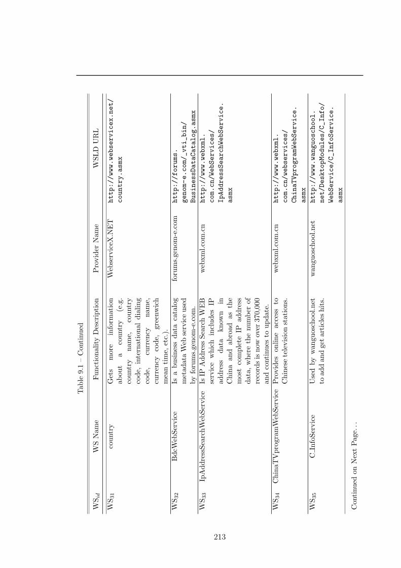
Tab
le9.
1–
Con
tinu
ed
WSid
WS
Nam
eF
un
ctio
nal
ity
Des
crip
tion
Pro
vid
erN
ame
WS
LD
UR
L
WS
31
cou
ntr
yG
ets
mor
ein
form
atio
nab
out
aco
untr
y(e
.g.
cou
ntr
yn
ame,
cou
ntr
yco
de,
inte
rnat
ion
ald
iali
ng
cod
e,cu
rren
cyn
ame,
curr
ency
cod
e,gr
eenw
ich
mea
nti
me,
etc.
).
Web
serv
iceX
.NE
Thttp://www.webservicex.net/
country.asmx
WS
32
Bd
cWeb
Ser
vic
eIs
ab
usi
nes
sd
ata
cata
log
met
adat
aW
ebse
rvic
eu
sed
by
foru
ms.
gen
om-e
.com
.
foru
ms.
gen
om-e
.com
http://forums.
genom-e.com/_vti_bin/
BusinessDataCatalog.asmx
WS
33
IpA
dd
ress
Sea
rch
Web
Ser
vic
eIs
IPA
ddre
ssS
earc
hW
EB
serv
ice
wh
ich
incl
ud
esIP
add
ress
dat
akn
own
inC
hin
aan
dab
road
asth
em
ost
com
ple
teIP
add
ress
dat
a,w
her
eth
enu
mb
erof
reco
rds
isn
owov
er37
0,00
0an
dco
nti
nu
esto
up
dat
e.
web
xm
l.co
m.c
nhttp://www.webxml.
com.cn/WebServices/
IpAddressSearchWebService.
asmx
WS
34
Ch
inaT
Vp
rogr
amW
ebSer
vic
eP
rovid
eson
lin
eac
cess
toC
hin
ese
tele
vis
ion
stat
ion
s.w
ebxm
l.co
m.c
nhttp://www.webxml.
com.cn/webservices/
ChinaTVprogramWebService.
asmx
WS
35
CIn
foS
ervic
eU
sed
by
wan
guos
chool
.net
toad
dan
dge
tar
ticl
esh
its.
wan
guos
chool
.net
http://www.wanguoschool.
net/DesktopModules/C_Info/
WebService/C_InfoService.
asmx
Con
tinu
edon
Nex
tP
age...
213

Tab
le9.
1–
Con
tinu
ed
WSid
WS
Nam
eF
un
ctio
nal
ity
Des
crip
tion
Pro
vid
erN
ame
WS
LD
UR
L
WS
36
kit
eser
vic
eU
sed
by
kit
esof
t.cn
toge
ta
loca
tion
by
IPad
drr
ess.
kit
esof
t.cn
http://www.kitesoft.cn/
services/kiteservice.asmx
WS
37
Ch
inaS
tock
Web
Ser
vic
eR
epor
tsti
mel
yC
hin
ese
stock
mar
ket
dat
a(s
tock
nam
e,p
rice
,..
.).
web
xm
l.co
m.c
nhttp://www.webxml.
com.cn/WebServices/
ChinaStockWebService.asmx?
wsdl
WS
38
pro
jnam
eU
sed
by
hzn
.sec
ond
hou
se.s
oufu
n.c
omto
man
age
the
exis
tin
gp
roje
cts
incl
ud
ing
gett
ing
the
nam
es,
cod
es,
and
pu
rpos
esof
the
pro
ject
s.
hzn
.sec
ond
hou
se.s
oufu
n.c
omhttp://hzn.secondhouse.
soufun.com/HouseService/
Estimate/projname.asmx?wsdl
WS
39
Wea
ther
Web
Ser
vic
eR
epor
tsw
eath
erfo
rm
ajo
rci
ties
inch
ina.
web
xm
l.co
m.c
nhttp://www.webxml.
com.cn/WebServices/
WeatherWebService.asmx?WSDL
WS
40
Ch
inaZ
ipS
earc
hW
ebS
ervic
eE
nab
les
tose
arch
ina
dat
abas
eco
nta
ins
all
the
zip
cod
eto
tal
of18
7,28
5re
cord
s,w
hic
his
the
mos
tco
mp
lete
Ch
ina
zip
cod
ed
ata.
web
xm
l.co
m.c
nhttp://www.webxml.
com.cn/WebServices/
ChinaZipSearchWebService.
asmx?wsdl
WS
41
WS
Mu
sic
Pro
vid
esd
iffer
ent
typ
eof
mu
sic
and
son
gs.
mic
roso
ft.c
omhttp://ws.contentlib.mweb.
co.th/ContentLibrary.WS/
WSMusic.asmx
Con
tinu
edon
Nex
tP
age...
214

Tab
le9.
1–
Con
tinu
ed
WSid
WS
Nam
eF
un
ctio
nal
ity
Des
crip
tion
Pro
vid
erN
ame
WS
LD
UR
L
WS
42
Am
azon
Box
Use
sA
maz
on.c
omW
ebS
ervic
esto
retu
rna
stri
ng
form
atte
dH
TM
Lta
ble
wit
hu
pto
9p
rod
uct
lin
ks
and
thei
ras
soci
ated
pri
ces,
imag
es,
and
man
ufa
ctu
r-er
s.A
llb
oxes
nee
don
lya
sin
gle
stri
ng
inp
ut
valu
e.A
nem
pty
HT
ML
tab
leis
retu
rned
ifn
ore
sult
sca
nb
ere
trie
ved
.S
eeth
eli
stb
elow
for
box
typ
esan
din
pu
tex
amp
les.
xm
lme.
com
http://www.xmlme.com/
WSAmazonBox.asmx
WS
43
Cop
yD
anS
ervic
eU
sin
gIS
SN
nu
mb
erre
-tu
rns
wea
ther
the
arti
cle
isa
scie
nti
fic
and
ther
efor
esu
bje
ctto
the
agre
emen
t.
stat
sbib
liot
eket
.dk
http://webservice.
statsbiblioteket.dk/
ws-ekopicopydan/services/
CopyDanServicePort?wsdl
WS
44
Rod
eoW
ebS
ervic
eU
sed
by
Lem
onte
chco
m-
pan
y,w
hic
his
spec
ial-
ized
inp
roje
ctd
evel
op-
men
tW
eb-b
ased
com
pu
t-in
g,to
coll
ect
info
rmat
ion
abou
tW
ebse
rvic
esan
dcl
assi
fyth
emin
majo
rli
sts
and
grou
ps.
lem
onte
ch.c
lhttp://rodeo.lemontech.cl/
rodeo/app/webservices.php?
wsdl
Con
tinu
edon
Nex
tP
age...
215

Tab
le9.
1–
Con
tinu
ed
WSid
WS
Nam
eF
un
ctio
nal
ity
Des
crip
tion
Pro
vid
erN
ame
WS
LD
UR
L
WS
45
Tra
inT
imeW
ebS
ervic
eP
rovid
esd
iffer
ent
trai
nsc
hed
ule
san
dst
atio
ns.
web
xm
l.co
m.c
nhttp://www.webxml.
com.cn/WebServices/
TrainTimeWebService.asmx
216

Bibliography
[1] H. Akaike. A new look at the statistical model identification. IEEE transactions onautomatic control, 19(6):716–723, 1974.
[2] E. Al-Masri and Q. H. Mahmoud. Discovering the best web service. In proceedingsof the 16th International Conference on World Wide Web, pages 1257–1258. ACM,2007.
[3] E. Al-Masri and Q. H. Mahmoud. Qos-based discovery and ranking of web services.In proceedings of 16th International Conference on Computer Communications andNetworks, pages 529–534. IEEE, 2007.
[4] J. Aldrich. Ra fisher and the making of maximum likelihood 1912-1922. StatisticalScience, 12(3):162–176, 1997.
[5] D. Ameller and X. Franch. Service level agreement monitor (salmon). In proceedingsof the Seventh International Conference on Composition-Based Software Systems(ICCBSS), pages 224–227. IEEE, 2008.
[6] A. Amendola, M. Niglio, and C. Vitale. The moments of setarma models. Statistics& probability letters, 76(6):625–633, 2006.
[7] F. Andre, E. Daubert, and G. Gauvrit. Towards a generic context-aware frameworkfor self-adaptation of service-oriented architectures. In proceedings of the Fifth Inter-national Conference on Internet and Web Applications and Services, pages 309–314.IEEE, 2010.
[8] V. Andrikopoulos, M. Fugini, M. Papazoglou, M. Parkin, B. Pernici, and S. Sia-dat. Qos contract formation and evolution. In proceedings of the 11th InternationalConference on Electronic Commerce and Web Technologies, pages 119–130, 2010.
[9] K. Appleby, S. Fakhouri, L. Fong, G. Goldszmidt, M. Kalantar, S. Krishnakumar,D. Pazel, J. Pershing, and B. Rochwerger. Oceano-SLA based management of acomputing utility. In proceedings of the IEEE/IFIP International Symposium onIntegrated Network Management, pages 855–868. IEEE, 2001.
[10] D. Ardagna, G. Giunta, N. Ingraffia, R. Mirandola, and B. Pernici. QoS-driven webservices selection in autonomic grid environments. In R. Meersman and Z. Tari,editors, On the Move to Meaningful Internet Systems 2006, volume 4276 of LectureNotes in Computer Science, pages 1273–1289. Springer, 2006.
217

[11] D. Ardagna and R. Mirandola. Per-flow optimal service selection for web servicesbased processes. The Journal of Systems and Software, 83(8):1512–1523, Aug. 2010.
[12] D. Ardagna and B. Pernici. Global and local QoS constraints guarantee in web ser-vice selection. In proceedings of the IEEE International Conference on Web Services(ICWS), pages 805–806. IEEE Computer Society, 2005.
[13] D. Ardagna and B. Pernici. Global and local QoS constraints guarantee in web ser-vice selection. In proceedings of the IEEE International Conference on Web Services(ICWS), pages 805–806. IEEE Computer Society, 2005.
[14] N. Artaiam and T. Senivongse. Enhancing service-side qos monitoring for web ser-vices. In proceedings of the International Conference on Software Engineering, Arti-ficial Intelligence, Networking, and Parallel/Distributed Computing, pages 765–770.IEEE, 2008.
[15] A. Aziz, K. Sanwal, V. Singhal, and R. K. Brayton. Verifying continuous timemarkov chains. In R. Alur and T. A. Henzinger, editors, proceedings of the 8thInternational Conference on Computer Aided Verification, volume 1102 of LNCS,pages 269–276. Springer, 1996.
[16] A. Baccigalupi, C. De Capua, and A. Liccardo. Overview on development of remoteteaching laboratories: from labview to web services. In proceedings of the IEEEInstrumentation and Measurement Technology Conference, pages 992–997. IEEE,2006.
[17] C. Baier, J.-P. Katoen, and H. Hermanns. Approximate symbolic model checking ofcontinuous-time markov chains. In J. C. M. Baeten and S. Mauw, editors, proceedingsof the 10th International Conference on Concurrency Theory, volume 1664 of LNCS,pages 146–161. Springer, 1999.
[18] R. Baragona, F. Battaglia, and D. Cucina. A note on estimating autoregressiveexponential models. Quaderni di Statistica, 4(1):71–88, 2002.
[19] R. Baragona, F. Battaglia, and D. Cucina. Estimating threshold subset autoregres-sive moving-average models by genetic algorithms. Metron-International Journal ofStatistics, 62(1):39–61, 2004.
[20] L. Baresi, E. Di Nitto, and C. Ghezzi. Toward open-world software: Issue andchallenges. Computer, 39(10):36–43, 2006.
[21] B. Behkamal, M. Kahani, and M. Akbari. Customizing iso 9126 quality model forevaluation of b2b applications. Information and software technology, 51(3):599–609,2009.
[22] A. Bellucci, V. Cardellini, V. Di Valerio, and S. Iannucci. A scalable and highly avail-able brokering service for sla-based composite services. Service-Oriented Computing,pages 527–541, 2010.
[23] R. Ben Halima, K. Guennoun, K. Drira, and M. Jmaiel. Non-intrusive qos moni-toring and analysis for self-healing web services. In proceedings of the International
218

BIBLIOGRAPHY
Conference on the Applications of Digital Information and Web Technologies, pages549–554. IEEE, 2008.
[24] R. Ben Halima, M. Guennoun, K. Drira, and M. Jmaiel. Providing Predictive Self-Healing for Web Services: A QoS Monitoring and Analysis-based Approach. Journalof Information Assurance and Security, 3(3):175–184, 2008.
[25] A. Benveniste, S. Haar, C. Jard, and S. Rosario. Qos monitoring of soft contractsfor transaction based web services orchestrations, 2008.
[26] R. Berbner, M. Spahn, N. Repp, O. Heckmann, and R. Steinmetz. Heuristics forQoS-aware web service composition. In proceedings of the IEEE International Con-ference on Web Services (ICWS), pages 72–82. IEEE Computer Society, 2006.
[27] R. Binder. Testing object-oriented systems: models, patterns, and tools. Addison-Wesley Professional, 2000.
[28] T. Bollerslev. Generalized autoregressive conditional heteroskedasticity. Journal ofEconometrics, 31(3):307–327, 1986.
[29] P. A. Bonatti and P. Festa. On optimal service selection. In A. Ellis and T. Hagino,editors, proceedings of the 14th international conference on World Wide Web, pages530–538. ACM, 2005.
[30] I. Bosloper, J. Siljee, J. Nijhuis, and D. Hammer. Creating self-adaptive servicesystems with dysoa. In proceedings of the Third IEEE European Conference on WebServices, pages 10–19. IEEE, 2005.
[31] D. Box, F. Curbera, M. Hondo, C. Kaler, D. Langworthy, A. Nadalin, N. Nagarat-nam, M. Nottingham, C. von Riegen, and J. Shewchuk. Web services policy frame-work (ws-policy), 2003.
[32] G. E. P. Box and D. R. Cox. An analysis of transformations. Journal of the RoyalStatistical Society. Series B (Methodological), 26(2):211–252, 1964.
[33] G. E. P. Box and G. M. Jenkins. Time Series Analysis: Forecasting and Control.HoldenDay, San Francisco, 1976.
[34] G. E. P. Box and D. A. Pierce. Distribution of residual autocorrelations inautoregressive-integrated moving average time series models. Journal of the Amer-ican Statistical Association, 65(332):1509–1526, 1970.
[35] T. S. Breusch and A. R. Pagan. A simple test for heteroscedasticity and randomcoefficient variation. Econometrica: Journal of the Econometric Society, pages 1287–1294, 1979.
[36] K. P. Burnham and D. R. Anderson. Model selection and multimodel inference: apractical information-theoretic approach. Springer-Verlag, 2002.
[37] R. Calinescu, L. Grunske, M. Z. Kwiatkowska, R. Mirandola, and G. Tamburrelli.Dynamic qos management and optimization in service-based systems. IEEE Trans.Software Eng., 37(3):387–409, 2011.
219

[38] L. L. Cam. Maximum likelihood: an introduction. International Statistical Review,pages 153–171, 1990.
[39] G. Canfora, M. D. Penta, R. Esposito, F. Perfetto, and M. L. Villani. Servicecomposition (re) binding driven by application–specific QoS. In proceedings of theinternational conference on Service-oriented computing, pages 141–152. Springer,2006.
[40] G. Canfora, M. D. Penta, R. Esposito, and M. L. Villani. An approach for QoS-awareservice composition based on genetic algorithms. In proceedings of the conference onGenetic and evolutionary computation, pages 1069–1075. ACM, 2005.
[41] G. Canfora, M. D. Penta, R. Esposito, and M. L. Villani. A framework for QoS-aware binding and re-binding of composite web services. Journal of Systems andSoftware, 81(10):1754–1769, 2008.
[42] V. Cardellini, E. Casalicchio, V. Grassi, S. Iannucci, F. Presti, and R. Mirandola.Moses: A framework for qos driven runtime adaptation of service-oriented systems.IEEE Transactions on Software Engineering, 38(5):1138–1159, 2012.
[43] V. Cardellini, E. Casalicchio, V. Grassi, F. Lo Presti, and R. Mirandola. Towardsself-adaptation for dependable service-oriented systems. Architecting DependableSystems VI, pages 24–48, 2009.
[44] V. Cardellini, E. Casalicchio, V. Grassi, and F. L. Presti. Flow-based service selec-tion for web service composition supporting multiple QoS classes. In proceedings ofthe IEEE International Conference on Web Services (ICWS), pages 743–750. IEEEComputer Society, 2007.
[45] V. Cardellini, E. Casalicchio, V. Grassi, and F. L. Presti. Scalable service selectionfor web service composition supporting differentiated QoS classes. Technical ReportTechnical Report RR-07.59, Dip. di Informatica, Sistemi e Produzione, Universitadi Roma Tor Vergata, 2007.
[46] B. Cavallo, M. D. Penta, and G. Canfora. An empirical comparison of methods tosupport QoS-aware service selection. In proceedings of the 2nd International Work-shop on Principles of Engineering Service-Oriented Systems, pages 64–70. ACM,2010.
[47] K. Chan. Consistency and limiting distribution of the least squares estimator of athreshold autoregressive model. The Annals of Statistics, 21(1):520–533, 1993.
[48] K. Chan, I. Poernomo, H. Schmidt, and J. Jayaputera. A model-oriented frameworkfor runtime monitoring of nonfunctional properties. Quality of Software Architecturesand Software Quality, pages 38–52, 2005.
[49] K. Chan and H. Tong. On likelihood ratio tests for threshold autoregression. Journalof the Royal Statistical Society. Series B (Methodological), pages 469–476, 1990.
[50] A. cheng Huang and P. Steenkiste. Building self-adapting services using service-specific knowledge. In proceedings of IEEE High Performance Distributed Comput-ing, pages 34–43. IEEE, 2005.
220

BIBLIOGRAPHY
[51] J. Cohen. Statistical power analysis for the behavioral sciences. Lawrence ErlbaumAssociates, Inc, 1988.
[52] J. Contreras, R. Espinola, F. J. Nogales, and A. J. Conejo. Arima models to predictnext-day electricity prices. IEEE Transactions on Power Systems, 18(3):1014–1020,2003.
[53] P. Cook and L. D. Broemeling. Analyzing threshold autoregressions with a bayesianapproach. Advances in Econometrics, 11:89–108, 1996.
[54] K. Czajkowski, A. Dan, J. Rofrano, S. Tuecke, and M. Xu. Agreement-based gridservice management (ogsi-agreement). In Version 0, Global Grid Forum, 2003.
[55] G. Dai and Y. Wang. A qos-aware web service orchestration engine based on actors.Advances in Computer Science and Information Engineering, pages 17–22, 2012.
[56] H. Daniels. Rank correlation and population models. Journal of the Royal StatisticalSociety. Series B (Methodological), 12(2):171–191, 1950.
[57] I. Daubechies. Orthonormal bases of compactly supported wavelets. Communica-tions on pure and applied mathematics, 41(7):909–996, 1988.
[58] F. David. A power function for tests of randomness in a sequence of alternatives.Biometrika, pages 335–339, 1947.
[59] R. de Lemos, H. Giese, H. Muller, M. Shaw, J. Andersson, L. Baresi, B. Becker,N. Bencomo, Y. Brun, B. Cikic, R. Desmarais, S. Dustdar, G. Engels, K. Geihs,K. M. Goeschka, A. Gorla, V. Grassi, P. Inverardi, G. Karsai, J. Kramer, M. Litoiu,A. Lopes, J. Magee, S. Malek, S. Mankovskii, R. Mirandola, J. Mylopoulos, O. Nier-strasz, M. Pezze, C. Prehofer, W. Schafer, W. Schlichting, B. Schmerl, D. B. Smith,J. P. Sousa, G. Tamura, L. Tahvildari, N. M. Villegas, T. Vogel, D. Weyns, K. Wong,and J. Wuttke. Software Engineering for Self-Adaptive Systems: A second ResearchRoadmap. In R. de Lemos, H. Giese, H. Muller, and M. Shaw, editors, SoftwareEngineering for Self-Adaptive Systems, number 10431 in Dagstuhl Seminar proceed-ings, Dagstuhl, Germany, 2011. Schloss Dagstuhl - Leibniz-Zentrum fuer Informatik,Germany.
[60] D. N. DeJong, J. C. Nankervis, N. E. Savin, and C. H. Whiteman. Integration versustrend stationary in time series. Econometrica: Journal of the Econometric Society,pages 423–433, 1992.
[61] P. Diaconis. Application of the method of moments in probability and statistics.Moments in Mathematics, 125:142, 1987.
[62] D. A. Dickey. Estimation and hypothesis testing in nonstationary time series. PhDthesis, Iowa State University Ames, 1976.
[63] D. A. Dickey and W. A. Fuller. Distribution of the estimators for autoregres-sive time series with a unit root. Journal of the American Statistical Association,74(366a):427–431, 1979.
221

[64] W.-L. Dong and H. Yu. Optimizing web service composition based on QoS negotia-tion. In proceedings of the Tenth IEEE International Enterprise Distributed ObjectComputing Conference, page 46. IEEE Computer Society, 2006.
[65] D. Dranidis, A. Metzger, and D. Kourtesis. Enabling proactive adaptation throughjust-in-time testing of conversational services. In proceedings of the Third Euro-pean Conference on Towards a Service-Based Internet, volume 6481, pages 63–75.Springer-Verlag New York Inc, 2010.
[66] J. Ehlers and W. Hasselbring. A self-adaptive monitoring framework for component-based software systems. Software Architecture, pages 278–286, 2011.
[67] W. Enders. Applied econometric time series. John Wiley & Sons, 2008.
[68] R. Engle. Autoregressive conditional heteroscedasticity with estimates of the vari-ance of united kingdom inflation. Econometrica, pages 987–1007, 1982.
[69] R. F. Engle, D. F. Hendry, and D. Trumble. Small-sample properties of arch esti-mators and tests. Canadian Journal of Economics, pages 66–93, 1985.
[70] I. Epifani, C. Ghezzi, and G. Tamburrelli. Change-point detection for black-boxservices. In proceedings of the eighteenth ACM SIGSOFT international symposiumon Foundations of software engineering, pages 227–236. ACM, 2010.
[71] F. Foster and A. Stuart. Distribution-free tests in time-series based on the breakingof records. Journal of the Royal Statistical Society. Series B (Methodological), pages1–22, 1954.
[72] S. Fu and C.-Z. Xu. Exploring event correlation for failure prediction in coalitionsof clusters. In proceedings of the ACM/IEEE conference on Supercomputing, pages1–12. ACM Press, 2007.
[73] S. Fu and C.-Z. Xu. Quantifying event correlations for proactive failure managementin networked computing systems. Journal of parallel and distributed computing,70(11):1100–1109, 2010.
[74] S. Gandhi. A service-oriented approach to b2b integration using web services.http://www.dreamscape.co.in. [Published for Dreamscape Media, last accessed:January 9, 2013].
[75] F. Garcıa-Sanchez, R. Valencia-Garcıa, R. Martınez-Bejar, and J. T. Fernandez-Breis. An ontology, intelligent agent-based framework for the provision of semanticweb services. Expert Systems with Applications, 36(2):3167–3187, 2009.
[76] P. Garthwaite, I. Jolliffe, and B. Jones. Statistical Inference. Oxford UniversityPress, 2002.
[77] J. D. Gibbons and S. Chakraborti. Nonparametric statistical inference. CRC, 2003.
[78] R. D. Gibbons. Use of combined shewhart-cusum control charts for ground watermonitoring applications. Ground water, 37(5):682–691, 1999.
222

BIBLIOGRAPHY
[79] R. L. Glass. The software-research crisis. IEEE Software, 11(6):42–47, 1994.
[80] M. Godse, U. Bellur, and R. Sonar. Automating QoS Based Service Selection. Inproceedings of the IEEE International Conference on Web Services, pages 534–541.IEEE, 2010.
[81] L. A. Goodman. Simplified runs tests and likelihood ratio tests for markoff chains.Biometrika, 45(1-2):181–197, 1958.
[82] K. Gottschalk, S. Graham, H. Kreger, and J. Snell. Introduction to web servicesarchitecture. IBM systems Journal, 41(2):170–177, 2002.
[83] C. Granger. A quick test for serial correlation suitable for use with non-stationarytime series. Journal of the American Statistical Association, 58(303):728–736, 1963.
[84] C. Granger and A. Andersen. An introduction to bilinear time series models. Van-denhoeck und Ruprecht, 1978.
[85] C. W. Granger and T. Terasvirta. Modelling non-linear economic relationships.OUP Catalogue, 1993.
[86] L. Grunske. An effective sequential statistical test for probabilistic monitoring.Information and Software Technology, 53(3):190 – 199, 2011.
[87] L. Grunske and P. Zhang. Monitoring probabilistic properties. In H. van Vliet andV. Issarny, editors, proceedings of the 7th joint meeting of the European Software En-gineering Conference and the International Symposium on Foundations of SoftwareEngineering, pages 183–192. ACM, 2009.
[88] N. Gunther. The practical performance analyst. Authors Choice Press, 2000.
[89] L. Hamel, M. Graiet, and W. Gaaloul. Event-b formalisation of web services fordynamic composition. In proceedings of the Eighth International Conference onSemantics, Knowledge and Grids (SKG), pages 150–156. IEEE, 2012.
[90] B. Hansen. Testing for linearity. Journal of Economic Surveys, 13(5):551–576, 1999.
[91] B. E. Hansen. The likelihood ratio test under nonstandard conditions: testing themarkov switching model of gnp. Journal of Applied Econometrics, 7:S61–S82, 1992.
[92] B. E. Hansen. Erratum: the likelihood ratio test under nonstandard conditions: test-ing the markov switching model of gnp. Journal of Applied Econometrics, 11(2):195–198, 1996.
[93] B. E. Hansen. Threshold effects in non-dynamic panels: Estimation, testing, andinference. Journal of Econometrics, 93(2):345–368, 1999.
[94] H. Hansson and B. Jonsson. A logic for reasoning about time and reliability. Formalaspects of computing, 6(5):512–535, 1994.
[95] D. Hawkins and D. Olwell. Cumulative sum charts and charting for quality improve-ment. Springer Verlag, 1998.
223

[96] S. Haykin. Neural Networks and Learning Machines: A Comprehensive Foundation.Prentice Hall, 2008.
[97] J. Hielscher, R. Kazhamiakin, A. Metzger, and M. Pistore. A framework for proactiveself-adaptation of service-based applications based on online testing. Towards aService-Based Internet, pages 122–133, 2008.
[98] M. O. Hilari. Quality of service (qos) in soa systems. a systematic review. Master’sthesis, Biblioteca Rector Gabriel Ferrate de la Universitat, Departamento LSI, 2009.
[99] O. Hili. Hellinger distance estimation of general bilinear time series models. Statis-tical Methodology, 5(2):119–128, 2008.
[100] B. Hobijn, P. H. Franses, and M. Ooms. Generalizations of the kpss-test for station-arity. Statistica Neerlandica, 58(4):483–502, 2004.
[101] J. R. Hosking. L-moments: analysis and estimation of distributions using linearcombinations of order statistics. Journal of the Royal Statistical Society. Series B(Methodological), pages 105–124, 1990.
[102] Z. Hua and B. Zhang. Improving density forecast by modeling asymmetric fea-tures: An application to s&p500 returns. European Journal of Operational Research,185(2):716–725, 2008.
[103] C. M. Hurvich and C.-L. Tsai. Regression and time series model selection in smallsamples. Biometrika, 76(2):297, 1989.
[104] IBM, Autonomic Computing. An architectural blueprint for autonomic computing,white paper, 2004.
[105] M. A. Ismail. Bayesian Forecasting for Nonlinear Time Series. PhD thesis, Univer-sity of Wales, Aberystwyth, Dyfed, 1994.
[106] ISO/IEC. International Standard 9126 Software Engineering – Product Quality,1991.
[107] M. Jaeger, G. Rojec-Goldmann, and G. Muhl. Qos aggregation for web service com-position using workflow patterns. In proceedings of the Eighth IEEE InternationalConference on Enterprise Distributed Object Computing, pages 149–159. IEEE, 2004.
[108] M. Jaeger, G. Rojec-Goldmann, and G. Muhl. Qos aggregation in web servicecompositions. In proceedings of the IEEE International Conference on e-Technology,e-Commerce and e-Service, pages 181–185. IEEE, 2005.
[109] G. Kapetanios. Threshold models for trended time series. Empirical Economics,28(4):687–707, 2003.
[110] G. Kapitsaki, D. Kateros, I. Foukarakis, G. Prezerakos, D. Kaklamani, and I. Ve-nieris. Service composition: State of the art and future challenges. In proceedings ofthe 16th Mobile and Wireless Communications Summit, pages 1–5. IEEE, 2007.
224

BIBLIOGRAPHY
[111] R. Kazhamiakin, S. Benbernou, L. Baresi, P. Plebani, M. Uhlig, and O. Barais.Adaptation of service-based systems. Service research challenges and solutions forthe future internet, pages 117–156, 2010.
[112] A. Keller and H. Ludwig. The wsla framework: Specifying and monitoring servicelevel agreements for web services. Journal of Network and Systems Management,11(1):57–81, 2003.
[113] K. Krishnamoorthy. Handbook of statistical distributions with applications, volume188. Chapman and Hall/CRC, 2010.
[114] K. Kritikos and D. Plexousakis. Requirements for qos-based web service descriptionand discovery. IEEE Transactions on Services Computing, 2(4):320–337, 2009.
[115] D. Kwiatkowski, P. Phillips, P. Schmidt, and Y. Shin. Testing the null hypothesis ofstationarity against the alternative of a unit root. Journal of Econometrics, 54:159–178, 1992.
[116] M. Ladan. Web services metrics: A survey and a classification. In proceedings ofthe International Conference on Network and Electronics Engineering, pages 93–98,2011.
[117] A. Lapadula, R. Pugliese, and F. Tiezzi. Using formal methods to develop ws-bpelapplications. Science of Computer Programming, 77(3):189–213, 2012.
[118] P. Leitner. Ensuring cost-optimal sla conformance for composite service providers.In proceedings of the ICSOC PhD Symposium, pages 43–48, 2009.
[119] P. Leitner, S. Dustdar, B. Wetzstein, and F. Leymann. Cost-based prevention ofviolations of service level agreements in composed services using self-adaptation.In proceedings of the ICSE Workshop on European Software Services and SystemsResearch: Results and Challenges (S-Cube), pages 34–35. IEEE, 2012.
[120] P. Leitner, W. Hummer, and S. Dustdar. Cost-based optimization of service com-positions. IEEE Transactions on Services Computing, 2011.
[121] P. Leitner, A. Michlmayr, F. Rosenberg, and S. Dustdar. Monitoring, predictionand prevention of sla violations in composite services. In proceedings of the IEEEInternational Conference on Web Services (ICWS), pages 369–376. IEEE, 2010.
[122] P. Leitner, B. Wetzstein, F. Rosenberg, A. Michlmayr, S. Dustdar, and F. Leymann.Runtime prediction of service level agreement violations for composite services. Inproceedings of the 3rd Workshop on Non-Functional Properties and SLA Manage-ment in Service-Oriented Computing, pages 176–186. Springer-Verlag, 2009.
[123] M. Li, J. Huai, and H. Guo. An Adaptive Web Services Selection Method Based onthe QoS Prediction Mechanism. In proceedings of the International Conference onWeb Intelligence and Intelligent Agent Technology, pages 395–402. IEEE, 2009.
[124] W. Li and K. Lam. Modelling asymmetry in stock returns by a threshold autore-gressive conditional heteroscedastic model. The Statistician, pages 333–341, 1995.
225

[125] Y. Liang, Y. Zhang, H. Xiong, and R. Sahoo. Failure prediction in ibm bluegene/levent logs. In proceedings of the Seventh IEEE International Conference on DataMining, pages 583–588. IEEE, 2007.
[126] K. Lim. On the stability of a threshold ar(1) without intercepts. Journal of TimeSeries Analysis, 13(2):119–132, 1992.
[127] L. K. Lim and M. McAleer. Convergence and catching up in asean: a comparativeanalysis. Applied Economics, 36(2):137–153, 2004.
[128] F. Liu, C. Li, and J. Yu. Description of web service composition model based on znotation. In proceedings of the International Conference on Computer Science andAutomation Engineering, volume 3, pages 587–591. IEEE, 2011.
[129] X. Liu, H. Song, and P. Romilly. An empirical investigation of the causal relationshipbetween openness and economic growth in china. Applied Economics, 29(12):1679–1686, 1997.
[130] Z. Liu, N. Gu, and G. Yang. A reliability evaluation framework on service ori-ented architecture. In proceedings of the 2nd International Conference on PervasiveComputing and Applications, pages 466–471. IEEE, 2007.
[131] G. Lodi. Middleware Services for Dynamic Clustering of Application Servers. Tech-nical report, Technical Report UBLCS-2006-06, PhD thesis, Univ. of Bologna, 2006.
[132] G. Lodi, F. Panzieri, D. Rossi, and E. Turrini. SLA-driven clustering of QoS-awareapplication servers. IEEE Transactions on Software Engineering, pages 186–197,2007.
[133] H. Ludwig, A. Keller, A. Dan, R. P. King, and R. Franck. Web service level agree-ment (wsla) language specification. IBM Corporation, pages 815–824, 2003.
[134] Y. Ma and B. Cukic. Adequate and precise evaluation of quality models in softwareengineering studies. In proceedings of the International ICSE Workshop on PredictorModels in Software Engineering (PROMISE), pages 1–1. IEEE, 2007.
[135] A. Maaradji. End-user service composition from a social networks analysis perspec-tive. PhD thesis, Institut National des Tlcommunications, 2011.
[136] A. E. Maganioti, H. D. Chrissanthi, P. C. Charalabos, R. D. Andreas, P. N. George,and C. N. Christos. Cointegration of event-related potential (erp) signals in exper-iments with different electromagnetic field (emf) conditions. Health, 2(5):400–406,2010.
[137] S. G. Makridakis, S. C. Wheelwright, and R. J. Hyndman. Forecasting methods andapplications. Wiley-India, 2008.
[138] J. S. Malak, M. Mohsenzadeh, and M. A. Seyyedi. Web Service QoS PredictionBased on Multi Agents. In proceedings of the International Conference on ComputerTechnology and Development, pages 265–269. IEEE, 2009.
226

BIBLIOGRAPHY
[139] L. Malinski and E. Bielinska. Statistical analysis of minimum prediction error vari-ance in the identification of a simple bilinear time-series model. Advances in SystemScience, Academic Publishing House EXIT, pages 183–188, 2010.
[140] S. Mallat. A Wavelet Tour of Signal Processing: The Sparse Way. Academic Press,2008.
[141] A. Mani and A. Nagarajan. Understanding quality of service for web services.http://www.ibm.com/developerworks/webservices/library/ws-quality/
index.html, January 2002. [Last accessed: January 9, 2013].
[142] H. B. Mann. Nonparametric tests against trend. Econometrica: Journal of theEconometric Society, pages 245–259, 1945.
[143] C. Martins. A note on the third-order moment structure of a bilinear model withnon-independent shocks. Portugaliae Mathematica, 56(1):115–126, 1999.
[144] M. Marzolla and R. Mirandola. Performance Aware Reconfiguration of SoftwareSystems. Technical report, Technical Report UBLCS-2010-11, Department of Com-puter Science, University of Bologna, 2010.
[145] I. Meedeniya, I. Moser, A. Aleti, and L. Grunske. Architecture-based reliability eval-uation under uncertainty. In 7th International Conference on the Quality of SoftwareArchitectures, QoSA 2011 and 2nd International Symposium on Architecting CriticalSystems, ISARCS 2011. Boulder, CO, USA, June 20-24, 2011, proceedings, pages85–94. ACM, 2011.
[146] A. B. S. Messaoud. Monitoring strategies for chatter detection in a drilling process.PhD thesis, University of Dortmund, Germany, 2006.
[147] A. Metzger. Towards accurate failure prediction for the proactive adaptation ofservice-oriented systems. In proceedings of the 8th workshop on Assurances for self-adaptive systems, pages 18–23. ACM, 2011.
[148] A. Metzger, O. Sammodi, and K. Pohl. Accurate proactive adaptation of service-oriented systems. In Assurances for Self-Adaptive Systems, pages 240–265. Springer,2013.
[149] A. Metzger, O. Sammodi, K. Pohl, and M. Rzepka. Towards pro-active adaptationwith confidence: Augmenting service monitoring with online testing. In proceedingsof the ICSE Workshop on Software Engineering for Adaptive and Self-ManagingSystems, pages 20–28. ACM, 2010.
[150] A. Metzger, E. Schmieders, O. Sammodi, and K. Pohl. Verification and testingat run-time for online quality prediction. In proceedings of the ICSE Workshop onEuropean Software Services and Systems Research: Results and Challenges (S-Cube),pages 49–50. IEEE, 2012.
[151] Y. H. Michlin, G. Y. Grabarnik, and E. Leshchenko. Comparison of the mean timebetween failures for two systems under short tests. IEEE Transactions on Reliability,58(4):589–596, 2009.
227

[152] A. Michlmayr. Event Processing in QoS-Aware Service Runtime Environments. PhDthesis, Vienna University of Technology, 2010.
[153] A. Michlmayr, F. Rosenberg, P. Leitner, and S. Dustdar. Comprehensive qos moni-toring of web services and event-based sla violation detection. In proceedings of the4th International Workshop on Middleware for Service Oriented Computing, pages1–6. ACM, 2009.
[154] A. Michlmayr, F. Rosenberg, P. Leitner, and S. Dustdar. End-to-end support forqos-aware service selection, binding, and mediation in vresco. IEEE Transactionson Services Computing, 3(3):193–205, 2010.
[155] Microsoft. WCF Performance Counters. http://msdn.microsoft.com/en-us/
library/ms735098.aspx, August 2012. [Last accessed: January 9, 2013].
[156] R. Mirandola and P. Potena. A qos-based framework for the adaptation of service-based systems. Scalable Computing: Practice and Experience, 12(1), 2011.
[157] D. C. Montgomery. Introduction to statistical quality control. Wiley-India, 2007.
[158] D. C. Montgomery, C. L. Jennings, and M. Kulahci. Introduction to time seriesanalysis and forecasting. John Wiley, 2008.
[159] D. C. Montgomery and G. C. Runger. Applied statistics and probability for engineers.New York; John Wiley, 2003.
[160] G. H. Moore and W. A. Wallis. Time series significance tests based on signs ofdifferences. Journal of the American Statistical Association, 38(222):153–164, 1943.
[161] A. Mosincat and W. Binder. Automated performance maintenance for service com-positions. In proceedings of the 11th IEEE International Symposium on Web SystemsEvolution, pages 131–140, 2009.
[162] A. Mosincat and W. Binder. Automated maintenance of service compositions withsla violation detection and dynamic binding. International Journal on SoftwareTools for Technology Transfer (STTT), 13(2):167–179, 2011.
[163] S. Mottaghi. Automatic black-box testing of gsm traffic in a simulated environment.Master’s thesis, Department of Numerical Analysis and Computing Science (NADA),Royal Institute of Technology (KTH), Stochkolm, 2005.
[164] C. R. Nelson and C. R. Plosser. Trends and random walks in macroeconmic timeseries: some evidence and implications. Journal of Monetary Economics, 10(2):139–162, 1982.
[165] D. Niu, Y. Wang, and D. Wu. Power load forecasting using support vector machineand ant colony optimization. Expert Systems with Applications, 37(3):2531–2539,2010.
[166] P. N. Nobile, R. R. F. Lopes, C. E. Moron, and L. C. Trevelin. QoS proxy archi-tecture for real time RPC with traffic prediction. In proceedings of the 11th IEEEInternational Symposium on Distributed Simulation and Real-Time Applications,pages 261–267. IEEE Computer Society, 2007.
228

BIBLIOGRAPHY
[167] C.-O. Oh. The contribution of tourism development to economic growth in thekorean economy. Tourism Management, 26(1):39–44, 2005.
[168] D. Okanovic, A. Hoorn, Z. Konjovic, and M. Vidakovic. Sla-driven adaptive mon-itoring of distributed applications for performance problem localization. ComputerScience and Information Systems, (00):37–37, 2012.
[169] Organization for the Advancement of Structured Information Standards (OASIS).Web Service Business Process Execution Language 2.0. http://docs.oasis-open.org/wsbpel/2.0/OS/wsbpel-v2.0-OS.html, April 2007. [Last accessed: January9, 2013].
[170] Organization for the Advancement of Structured Information Standards (OA-SIS). Universal Description, Discovery and Integration (UDDI). http://www.
oasis-open.org/committees/uddi-spec/, February 2005. [Last accessed: Jan-uary 9, 2013].
[171] T. Ozaki. Non-linear time series models for non-linear random vibrations. Journalof applied probability, pages 84–93, 1980.
[172] T. Ozaki. Non-linear time series models and dynamical systems, volume 5. North-Holland, Amsterdam, 1985.
[173] T. Ozaki and H. Oda. Non-linear time series model identification by akaike’s infor-mation criterion. In proceedings of the IFAC workshop on Information and Systems,pages 83–91. Compiegne, France, 1978.
[174] E. Page. Continuous inspection schemes. Biometrika, 41(1-2):100–115, 1954.
[175] A. Pankratz. Forecasting with univariate Box-Jenkins models: Concepts and cases.New York; Wiley, 1983.
[176] M. P. Papazoglou and W.-J. van den Heuvel. Service oriented architectures: ap-proaches, technologies and research issues. The VLDB Journal, 16(3):389–415, 2007.
[177] M. Parker. Integration of active and passive monitoring technologies into care ser-vices. Gerontechnology, 9(2):159, 2010.
[178] M. Parkin and A. Metzger. Initial set of principles, techniques and methodologiesfor assuring end-to- end quality and monitoring of slas. Technical report, DeliverableCD-JRA-1.3. 4, S-Cube Consortium, 2010.
[179] C. Peltz. Web services orchestration and choreography. Computer, 36(10):46–52,2003.
[180] B. Pernici and S. Siadat. Adaptation of web services based on qos satisfaction. Inproceedings of the International Conference on Service-Oriented Computing, pages65–75. Springer, 2010.
[181] B. Pernici and S. Siadat. A fuzzy service adaptation based on qos satisfaction. Inproceedings of the 23rd International Conference on Advanced Information SystemsEngineering (CAiSE), volume 6741, pages 48–61. Springer, 2011.
229

[182] J. Petruccelli. On the approximation of time series by threshold autoregressivemodels. Sankhya: The Indian Journal of Statistics, pages 106–113, 1992.
[183] J. Petruccelli and N. Davies. A portmanteau test for self-exciting thresholdautoregressive-type nonlinearity in time series. Biometrika, 73(3):687–694, 1986.
[184] M. Priestley. Non-linear and non-stationary time series analysis. Academic Press,1988.
[185] P. Qiu. Generalized least squares. Technometrics, 47(4):519–519, 2005.
[186] F. Raimondi, J. Skene, and W. Emmerich. Efficient online monitoring of web-service SLAs. In proceedings of the 16th ACM SIGSOFT International Symposiumon Foundations of software engineering, pages 170–180, New York, NY, USA, 2008.ACM Press.
[187] S. Ran. A model for web services discovery with qos. ACM Sigecom exchanges,4(1):1–10, 2003.
[188] J. Rao and X. Su. A survey of automated web service composition methods. InSemantic Web Services and Web Process Composition, pages 43–54. Springer, 2005.
[189] Y. Raymond. An application of the arima model to real-estate prices in hong kong.Journal of Property Finance, 8(2):152–163, 1997.
[190] N. Regnard and J.-M. Zakoian. A conditionally heteroskedastic model with time-varying coefficients for daily gas spot prices. Energy Economics, 33(6):1240–1251,2011.
[191] G. Ribeiro-Justo and A. Saleh. Non-functional integration and coordination of dis-tributed component services. In proceedings of the Sixth European Conference onSoftware Maintenance and Reengineering, pages 126–133. IEEE, 2002.
[192] S. Rosario, A. Benveniste, S. Haar, and C. Jard. Probabilistic qos and soft contractsfor transaction-based web services orchestrations. IEEE Transactions on ServicesComputing, 1(4):187–200, 2008.
[193] F. Rosenberg. QoS-Aware Composition of Adaptive Service-Oriented Systems. PhDthesis, Vienna University of Technology, 2009.
[194] F. Rosenberg, C. Platzer, and S. Dustdar. Bootstrapping performance and depend-ability attributes ofweb services. In proceedings of the IEEE International Confer-ence on Web Services (ICWS), pages 205–212. IEEE, 2006.
[195] R. Rouvoy, P. Barone, Y. Ding, F. Eliassen, S. Hallsteinsen, J. Lorenzo, A. Mamelli,and U. Scholz. Music: Middleware support for self-adaptation in ubiquitous andservice-oriented environments. Software Engineering for Self-Adaptive Systems,pages 164–182, 2009.
[196] D. Rud, A. Schmietendorf, and R. Dumke. Resource metrics for service-orientedinfrastructures. proceedings of the Workshop on Software Engineering Methods forService-Oriented Architecture, pages 90–98, 2007.
230

BIBLIOGRAPHY
[197] S. E. Said and D. A. Dickey. Testing for unit roots in autoregressive-moving averagemodels of unknown order. Biometrika, 71(3):599–607, 1984.
[198] M. Salehie and L. Tahvildari. Self-adaptive software: Landscape and research chal-lenges. ACM Transactions on Autonomous and Adaptive Systems (TAAS), 4(2):1–42, 2009.
[199] F. Salfner, M. Lenk, and M. Malek. A survey of online failure prediction methods.ACM Computing Surveys (CSUR), 42(3):10, 2010.
[200] U. Sammapun, I. Lee, and O. Sokolsky. RT-MaC: Runtime monitoring and check-ing of quantitative and probabilistic properties. In proceedings of the 11th IEEEInternational Conference on Embedded and Real-Time Computing Systems and Ap-plications, pages 147–153, 2005.
[201] U. Sammapun, I. Lee, O. Sokolsky, and J. Regehr. Statistical runtime checking ofprobabilistic properties. In Runtime Verification, pages 164–175. Springer, 2007.
[202] O. Sammodi, A. Metzger, X. Franch, M. Oriol, J. Marco, and K. Pohl. Usage-basedonline testing for proactive adaptation of service-based applications. In proceedingsof the IEEE 35th Annual Computer Software and Applications Conference (COMP-SAC), pages 582–587. IEEE, 2011.
[203] M. Sathya, M. Swarnamugi, P. Dhavachelvan, and G. Sureshkumar. Evaluation ofqos based web-service selection techniques for service composition. InternationalJournal of Software Engineering, 1(5):73–90, 2010.
[204] E. Schmieders and A. Metzger. Preventing performance violations of service com-positions using assumption-based run-time verification. In proceedings of the 4thEuropean Conference on Towards a Service-Based Internet, volume 6994, page 194.Springer, 2011.
[205] B. Schroeder and G. A. Gibson. A large-scale study of failures in high-performancecomputing systems. Dependable and Secure Computing, IEEE Transactions on,7(4):337–350, 2010.
[206] F. Schulz. Towards Measuring the Degree of Fulfillment of Service Level Agreements.In proceedings of the Third International Conference on Information and Computing,pages 273–276. IEEE, 2010.
[207] Seekda.com. http://webservices.seekda.com/. [Last accessed: January 9, 2013].
[208] R. Serral-Gracia, Y. Labit, J. Domingo-Pascual, and P. Owezarski. Towards anefficient service level agreement assessment. In proceedings of the International Con-ference on Computer Communications, pages 2581–2585. IEEE, 2009.
[209] M. Shaw. What makes good research in software engineering? International Journalon Software Tools for Technology Transfer, 4(1):1–7, 2002.
[210] W. A. Shewhart. Economic control of quality of manufactured product. New York:Van Nostrand, 1931.
231

[211] Z. Shi and H. Aoyama. Estimation of the exponential autoregressive time seriesmodel by using the genetic algorithm. Journal of Sound and Vibration, 205(3):309–321, 1997.
[212] Z. Shi, Y. Tamura, and T. Ozaki. A study on real-time detecting of machinetool chatter. International journal of the Japan Society for Precision Engineering,32:178–182, 1998.
[213] C. Shirky. Planning for Web Services: Obstacles & Opportunities. O’Reilly, 2002.
[214] R. H. Shumway and D. S. Stoffer. Time series analysis and its applications. SpringerScience, 2010.
[215] J. Siljee, I. Bosloper, J. Nijhuis, and D. Hammer. Dysoa: making service systemsself-adaptive. In proceedings of the International Conference on Service-OrientedComputing, pages 255–268. Springer, 2005.
[216] J. Simmonds, Y. Gan, M. Chechik, S. Nejati, B. O’Farrell, E. Litani, and J. Water-house. Runtime monitoring of web service conversations. IEEE T. Services Com-puting, 2(3):223–244, 2009.
[217] J. Skene, A. Skene, J. Crampton, and W. Emmerich. The monitorability of service-level agreements for application-service provision. In V. Cortellessa, S. Uchitel, andD. Yankelevich, editors, proceedings of the 6th International Workshop on Softwareand Performance, pages 3–14. ACM, 2007.
[218] A. Solomon and M. Litoiu. Business process performance prediction on a trackedsimulation model. In proceedings of the 3rd international workshop on Principles ofengineering service-oriented systems, pages 50–56. ACM, 2011.
[219] J. Sommers, P. Barford, N. Duffield, and A. Ron. Accurate and efficient sla com-pliance monitoring. In proceedings of the International Conference on Applications,Technologies, Architectures, and Protocols for Computer Communications, pages109–120, 2007.
[220] Z. G. Stoumbos, M. R. Reynolds, T. P. Ryan, and W. H.Woodall. The state of sta-tistical process control as we proceed into the 21st century. Journal of the AmericanStatistical Association, 95(451):992–998, 2000.
[221] T. Subba Rao. On the theory of bilinear time series models. Journal of the RoyalStatistical Society, 43(2):244–255, 1981.
[222] R. Sumra and D. Arulazi. Quality of service for web services-demystification, limi-tations, and best practices. http://www.developer.com/services/article.php/2027911, March 2003. [Last accessed: January 9, 2013].
[223] Z. Tan, J. Zhang, J. Wang, and J. Xu. Day-ahead electricity price forecastingusing wavelet transform combined with arima and garch models. Applied Energy,87(11):3606–3610, 2010.
232

BIBLIOGRAPHY
[224] P. Thongtra and F. A. Aagesen. An autonomic framework for service configura-tion. In proceedings of the Sixth International Multi-Conference on Computing inthe Global Information Technology, pages 116–124, 2011.
[225] H. Tong. Threshold models in non-linear time series analysis, volume 21. Springer,1983.
[226] H. Tong. Non-linear time series: a dynamical system approach. Oxford UniversityPress, 1990.
[227] H. Tong. Non-linear time series: a dynamical system approach, volume 6. OxfordUniversity, 1993.
[228] H. Tong and K. Lim. Threshold autoregression, limit cycles and cyclical data.Journal of the Royal Statistical Society. Series B (Methodological), pages 245–292,1980.
[229] V. Torres, V. Pelechano, M. Ruiz, and P. Valderas. A model driven approach for theintegration of external functionality in web applications. the travel agency system. Inproceedings of the Workshop on Model-driven Web Engineering, pages 1–11. Citeseer,2005.
[230] R. S. Tsay. Testing and modeling threshold autoregressive processes. Journal of theAmerican Statistical Association, 84(405):231–240, 1989.
[231] L.-H. Vu, M. Hauswirth, and K. Aberer. QoS-based service selection and rankingwith trust and reputation management. In proceedings of the international confer-ence on Cooperative Information Systems, pages 466–483. Springer, 2005.
[232] A. Wald. Sequential tests of statistical hypotheses. The Annals of MathematicalStatistics, pages 117–186, 1945.
[233] A. Wald and J. Wolfowitz. On a test whether two samples are from the samepopulation. The Annals of Mathematical Statistics, pages 147–162, 1940.
[234] A. Wald and J. Wolfowitz. An exact test for randomness in the nonparametric casebased on serial correlation. The Annals of Mathematical Statistics, pages 378–388,1943.
[235] H. Wang, X. Zeng, L. Deng, and Y. Guo. Design of the web-servers monitoringsystem based on ace framework. Applied Mechanics and Materials, 198:439–443,2012.
[236] L. Wang, J. Shen, and J. Yong. A survey on bio-inspired algorithms for web servicecomposition. In proceedings of the IEEE 16th International Conference on ComputerSupported Cooperative Work in Design (CSCWD), pages 569–574. IEEE, 2012.
[237] M. Weske. Business process management architectures. Business Process Manage-ment, pages 333–371, 2012.
[238] H. White. A heteroskedasticity-consistent covariance matrix estimator and a directtest for heteroskedasticity. Econometrica: Journal of the Econometric Society, pages817–838, 1980.
233
[239] World Wide Web Consortium (W3C). Simple Object Access Protocol (SOAP) v1.2.http://www.w3.org/TR/soap12/, April 2007. [Last accessed: January 9, 2013].
[240] World Wide Web Consortium (W3C). Web Services Architecture. http://www.w3.org/TR/ws-arch/, February 2004. [Last accessed: January 9, 2013].
[241] World Wide Web Consortium (W3C). Web Service Description Language (WSDL)v2.0. http://www.w3.org/TR/wsdl20/, June 2007. [Last accessed: January 9,2013].
[242] World Wide Web Consortium (W3C). QoS for Web Services: Requirements and Pos-sible Approaches. http://www.w3c.or.kr/kr-office/TR/2003/ws-qos/, Novem-ber 2003. [Last accessed: January 9, 2013].
[243] World Wide Web Consortium (W3C). Web Services Choreography Description Lan-guage Version 1.0. http://www.w3.org/TR/ws-cdl-10/, November 2005. [Lastaccessed: January 9, 2013].
[244] H. Younes and R. Simmons. Probabilistic verification of discrete event systems usingacceptance sampling. In Computer Aided Verification, pages 23–39. Springer, 2002.
[245] L. Yu, Z. Zheng, Z. Lan, and S. Coghlan. Practical online failure prediction forblue gene/p: Period-based vs event-driven. In proceedings of the IEEE/IFIP 41stInternational Conference on Dependable Systems and Networks Workshops, pages259–264. IEEE, 2011.
[246] J. Zeng. A case study on applying itil availability management best practice. Con-temporary Management Research, 4(4):321–332, 2008.
[247] L. Zeng, B. Benatallah, M. Dumas, J. Kalagnanam, and Q. Z. Sheng. Qualitydriven web services composition. In proceedings of the 12th international conferenceon World Wide Web, pages 411–421. ACM, 2003.
[248] L. Zeng, B. Benatallah, A. H. Ngu, M. Dumas, J. Kalagnanam, and H. Chang. QoS-aware middleware for web services composition. IEEE Transactions on SoftwareEngineering, 30(5):311–327, 2004.
[249] L. Zeng, H. Lei, and H. Chang. Monitoring the QoS for Web Services. In proceedingsof the Fifth International Conference on Service-oriented Computing, pages 132–144.Springer-Verlag New York Inc, 2007.
[250] L. Zeng, C. Lingenfelder, H. Lei, and H. Chang. Event-driven quality of serviceprediction. In proceedings of the 6th International Conference on Service-orientedComputing, pages 147–161. Springer-Verlag, 2008.
[251] L. Zeng, Y. Zhang, and X. Zhao. Storage performance optimization based on arima.In proceedings of the First International Workshop on Database Technology andApplications, pages 377–381. IEEE, 2009.
[252] Z. Zhang and S. Fu. Failure prediction for autonomic management of networked com-puter systems with availability assurance. In proceedings of the International Sympo-sium on Parallel & Distributed Processing, Workshops and Phd Forum (IPDPSW),pages 1–8. IEEE, 2010.
234

BIBLIOGRAPHY
[253] H. Zheng, J. Yang, W. Zhao, and A. Bouguettaya. Qos analysis for web servicecompositions based on probabilistic qos. In proceedings of the 9th InternationalConference on Service Oriented Computing, volume 7084, pages 47–61. Springer,2011.
[254] Z. Zheng. QoS Management of Web services. PhD thesis, Chinese University ofHong Kong, 2011.
[255] Z. Zheng and M. R. Lyu. Collaborative reliability prediction for service-oriented sys-tems. In proceedings of the IEEE/ACM 32nd International Conference on SoftwareEngineering, pages 35–44, 2010.
[256] Z. Zheng, Y. Zhang, and M. Lyu. Distributed qos evaluation for real-world webservices. In proceedings of the IEEE International Conference on Web Services(ICWS), pages 83–90. IEEE, 2010.
[257] S. Zhu, Z. Du, Y. Chen, X. Chai, and B. Li. QoS Enhancement for PDES GridBased on Time Series Prediction. In proceedings of the 6th International Conferenceon Grid and Cooperative Computing, pages 423–429. IEEE, 2007.
[258] S. Zribi, F. Benaben, A. Hamida, and J. Lorre. Towards a service and choreographygovernance framework for future internet. Enterprise Interoperability V, pages 281–291, 2012.
235